from principle-based risk management to solvency - scor
TRANSCRIPT

From Principle-BasedRisk Management to
Solvency Requirements
Analytical Framework for the Swiss Solvency Test
SCOR Switzerland AG∗
2nd Edition, 2008
∗General Guisan-Quai 26, 8002 Zurich SwitzerlandPhone +41 44 639 9393 Fax +41 44 639 9090

Copyright 2008 by SCOR Switzerland AGAll rights reserved. Any duplication, further processing, republishing or redistribution of the present book”From Principle-based Risk Management to Solvency Requirements”, in whole or in part, is not allowed withoutprior written consent by SCOR Switzerland AG.

Table of Contents
Prefaces iv
Acknowledgements viii
List of Contributors x
Executive Summary xii
I Insurance Risk 1
II Market Risk 192
III Credit Risk 296
IV Operational and Emerging Risks 323
V The Economic Balance Sheet 328
VI Solvency Capital Requirements 350
VII Process Landscape 352
VIII SST Systems 407
IX Final Remarks 450
ii


The merger of the SCOR group with Converium brought about, as partof the “wedding arrangement”, a well-advanced corporate asset and liabil-ity management according to the requirements of the Swiss Solvency Test(SST).
Putting into place and making such a significant project work, requiresthe collaboration of a variety of highly skilled professionals, who bring alongmany years of work experience in the various fields of the project. The factof sharing this broad knowledge is already an asset to the company processes.
It is important to acknowledge the competence and the attention to qual-ity which have guided the management of this project. In reading this book,anyone can appreciate the quality of work done and the competence of theproject’s participants who compiled this extensive SST documentation.
Beyond the accomplishment of the Zurich entity, which is remarkable initself, the SCOR group finds it a very useful experience for its other Eu-ropean entities. This will enable the group to comply with the risk modelrequired by Solvency II in the future, which is based on concepts very closeto those of the SST. For satisfying the future requirements by the EuropeanUnion’s regulations, the rapid implementation of the SST will allow us tobring valuable experience to the group for choosing the appropriate toolsand methods going forward.
Thus, the important investment and the accumulation of knowledgemade over time by the teams of SCOR Switzerland (former Converium)will enable us not only to satisfy the expectations of the Swiss regulator butundoubtedly represent an advantage for the SCOR group as a whole.
Beyond the regulatory requirements, the understanding of the conceptsas well as results of risk modeling is essential in all sectors of the group. Thewhole set of rules, processes, and methods that accompany the implemen-tation of those models are vital in developing a coherent Entreprise RiskManagement process. This process allows the company to optimally allo-
vi

cate the capital necessary for the business; a framework of a successful andcoherent risk and reward strategy.
This decisive step for the future of the group is now operational. Here-with we would like to thank all the people who have contributed to the SSTdocumentation, in particular Michel Dacorogna and his team whose talentand enthusiasm have brought this project to a successful end which wascomplex by nature and required careful and skilful handling.
Jean-Luc BessonChief Risk OfficerSCOR Group
April, 2008
vii
Acknowledgements
This documentation is a testimony to the long-term commitment of ZurichRe, Converium and SCOR with regard to the development of strong quan-titative tools and processes for managing the risks of our company. Thisfive hundred page book describes the results of many years of discussionsand work on the best way to model the great variety of risks in a reinsur-ance company. The Swiss Solvency Test (SST) required us to describe ourmodels and processes and gave us the opportunity to look back criticallyat all the developments in those areas. When it comes to acknowledgingthe many contributions, it is difficult not to forget someone, since so manypeople were involved in this large project over the years.
First of all our thanks go out to all the contributors of this book who arealso listed in a separate section. They have spent time and energy and showntheir enthusiasm in describing the content of their daily work. Markus Gutwas responsible for editing the modelling part. Although coming from a verydifferent background, he gained the respect of the experts he worked withthrough his dedication and diligence he brought to this task. The qualityof the set up of this documentation testifies to his important contribution.Martin Skalsky was the editor for the process part. Thanks to his quickgrasp of the facts and his independent view, he managed to describe theSST-related processes in easily comprehensible and illustrative ways. Hewas supported by Roland Burgi who added the technical element thanks tohis thorough understanding of processes and systems. Roland was also theauthor of the system description which demonstrates his qualities as a sys-tem architect. The executive summary was written by Michael Moller. Histechnical know-how as well as his detailed knowledge of the internal modelwere indispensable in the description of the concept the model is built on.All the other experts cited in the list of contributors have produced equallyhigh quality descriptions of their areas of responsibilities that make this texta living document explaining in great detail the various aspects of modellingour business.
We would also like here to acknowledge the work of all the membersof the SST core team who have contributed to the progress of the project
viii

and gave their support to this long-term effort over the years since April2006. The members of the steering committee have been a great supportfor this endeavour. We want to particularly thank Andy Zdrenyk and Paolode Martin whose strong support reflected the importance of this documen-tation for the entire company. Last but not least, we would like to pointout the two project managers who accompanied us along these months withtheir commitment and dedication through all the ups and downs of such ademanding project: Jindrich Wagner and Viviane Engelmayer.
You all made this project possible and gave us a sense of pride for thedevelopment of our internal model and its enhancements that will ultimatelyallow us to fulfil the regulators’ requirements.
Michel DacorognaHead of Group Financial ModelingSCOR Group
April, 2008
ix

List of Contributors
NAME FUNCTION COMPANY
Blum Peter Research Associate SCORBurgi Roland Senior Risk Consultant SCORDacorogna Michel Head of Financial
ModelingSCOR
de Braaf Karsten Life Actuary SCORDossena Miriam Risk Consultant SCOREngelmayer Viviane SST Project Manager SCORErixon Erik Consultant Towers PerrinGallati Livia Legal Counsel SCORGose Bernhard Consultant Towers PerrinGrutzner Guido Life Actuary SCORGut Markus Documentation Editor SCORHeil Jan Investment Controller SCORHomrighausen Jost Life Actuary SCORHummel Christoph Actuarial Risk Modeling SCORIannuzzi Debora Risk Consultant SCORJager Markus Life Actuary and
Risk ManagerSCOR
Kalberer Tigran Principal Towers PerrinKuttel Stefan Head of Pricing Zurich &
CologneSCOR
Langer Bernd Chief Risk Officer GlobalP&C
SCOR
Matter Flavio Cat Risk Analyst SCORMohr Christoph Actuarial Risk Modeling SCORMoller Michael Senior Risk Consultant SCORMuller Ulrich Senior Risk Consultant SCORPabst Brigitte Cat Risk Analyst SCORRuttener Erik Head of Natural Hazards SCOR
x

NAME FUNCTION COMPANY
Schindler Christine Publisher SCORSkalsky Martin Documentation Editor SCORTrachsler Michael Pricing Actuary SCORWagner Jindrich SST Project Manager SCORWallin Ake Head of Global IT
DevelopmentSCOR
Wollenmann Beatrice Pricing Actuary SCORZbinden Andreas Senior Cat Risk Analyst SCOR
xi
Executive Summary
This SST-model documentation will give the reader of the SST report theorientation about the origin, purpose and interpretation of the results stem-ming from SCOR’s internal model . As the results of the internal modelare used by SCOR’s top management for their decision findings, a clearunderstanding of the model framework should be supported by this docu-mentation. To mention some of the major decisions backed by the internalmodel results, there are the need for the overall capital and hybrid debtrequirements (implying an assessment of the equity dimension of hybridinstruments), the strategic asset allocation (based on different risk-returnoutcomes of the company’s value depending on different asset allocations),the capital allocation to major risk sources (based on the contributions to theoverall risk of a risk driver) and, therefore, the future direction of SCOR’sbusiness and, last but not least, risk mitigation measures (such as the impactof retrocession programmes).
However, the focus of the SST-Report lies in the thorough investigationand analysis of the Solvency capital requirements (SCR), i.e. the differencebetween risk-bearing capital and target capital, based on the valuation of theeconomic balance sheet of the legal entities of the company at the beginningand the end of the related period.
The definitions of the terms related to the SCR are outlined in severaldocuments published by the FOPI (see, for instance, “Technisches Doku-ment zum Swiss Solvency Test” Version 2 October 2006, p. 3/4 and also inPart I of this documentation). In general, risk-bearing capital is measuredas the difference of the market value of assets and the best estimate of lia-bilities assuming a run-off perspective after one year, even if some assets orliabilities are not on the formal balance sheet after one year, e.g. embeddedvalue of the life business, whereas the target capital requirement is computedas the difference between the expected economic risk-bearing capital at thebeginning of the period and the expected shortfall at risk tolerance level1% of the risk-bearing capital at the end of the period under considerationplus the cost of capital required to settle the associated run-off portfolio, i.e.the market value margin (MVM).
Any assessment of the future development of assets and liabilities de-pending on all relevant risk factors is based on a Monte Carlo simulation
xii

approach. The major risk factor categories set by the FOPI comprise insur-ance risk , market risk and credit risk which are further split into several sub-risks. Many scenarios are stochastically generated for all these individualrisk factors and applied to the affected economic balance sheet quantities byaggregating the individual items using a hierarchical copula-dependency treeapproach for the new business risk, correlation for the dependencies betweenrun-off lobs and regression-type dependencies between assets and liabilities,if necessary. It has to be noted that the different risks are consistently gen-erated and their mutual dependence is fully taken into consideration. Otherrisks like operational risk or liquidity risk are also considered in the inter-nal model but are partly not (yet) included in the detailed SCR calculations.
The general outline of this documentation is as follows: The first threeparts of this SST-documentation investigate in detail the modeling ap-proaches for the insurance, market and credit risk. Part IV deals withoperational risk and emerging risks. Part V describes the valuation of theeconomic balance-sheet items from the output perspective. The resultingeconomic shareholders-equity position (or “ultimate” economic valuation ofthe legal entity) constitutes the basis for the ultimate SCR computationsthat are outlined in Part VI. The last part will give the reader a briefoverview on qualitative risk factors that are analyzed in the context of ERMbut not explicitly considered for the SST from a quantitative point of view.It finishes with an outlook to further enhancements of the model that areenvisaged in the short to mid-term.
The internal modeling of the insurance risk affects several dimensions.The main categories are Life versus Non-life risks and New business versusRun-off risks, respectively. Non-Life insurance risks are generally modeledas aggregate loss distributions per major line of business (e.g. Motor, Li-ability, Property and Property Cat). The aggregate loss distribution of aline of business is itself the convolution of the ultimate loss distributions percontract level. The aggregation process of all the loss distributions followsa hierarchical dependency tree that assumes at each of its nodes a copuladependency.
For lines of business with major excess of loss retrocession, a frequency-severity distribution model approach is used. A very important example ofthis is currently (i.e. 2007) SCOR’s cat business where cat frequency scenar-ios are linked to the regional severity distribution which is itself a functionof the underlying exposure data. Details related to the modeling of the natcat risks can be found in Section 3.8. The Credit & Surety loss model isbased on a compound Poisson loss model. For details on the generation ofthe probability to default and the loss given default distribution the readermay refer to Section 3.6.
xiii
The Non-Life Run-off risk is basically modeled using the Merz-Wuthrichapproach (Section 3.9 of this documentation). Contrary to the originalMack-method estimating reserve risk volatility based on the ultimate reserverisk, the Merz-Wuthrich approach focuses on the reserve risk volatility ofthe one year change (“volatility of the triangle diagonal”) which is the ap-propriate view from the SST perspective.
Several sub-risk models have been built for the Life risk, see Chapter 4 fordetails. The main building blocks are risk models for guaranteed minimumdeath benefits (GMDB), Financial Reinsurance, Fluctuation risk, trend riskand life reserve risk. The GMDB-exposure is in general affected by capitalmarket risks and therefore modeled using a replicating portfolio. The otherinherent risks, namely mortality risk and policyholder behavior are eitherdeemed immaterial or modeled together with other risk buckets. The cur-rent Financial Reinsurance contracts mainly exhibit credit risk as the cedentcould eventually go bust. Other risks like higher mortality or higher lapserates are negligible due to the specific contract features. Stochastic creditdefaults stemming from the credit risk model are applied to the determinis-tic cash flow projection of the non-default case of the financial reinsurance.Trend risk mainly (e.g. parameter uncertainty) affects long-duration busi-ness and is modeled as the distribution of NPVs of future stochastic cashflows. Fluctuation risk resulting from morbidity, mortality or accident risksis modeled as an aggregate loss distribution and relates especially to short-and long duration business to reflect short-term loss variability.
Capital allocation is provided according to the contribution to expectedshortfall principle, see Section 8.3.
The market risk, i.e. the risk of changes of the economic environment,relates primarily, but not exclusively, to the economic value change of theinvested assets of the company. Of course, the change in interest rates affectseconomically all balance sheet positions that are or have to be discounted likenon-life reserves or reinsurance assets and the valuation of bond investmentsor interest rate hedges simultaneously.
Most important changes of the market environment are related to achange in interest rates, a drop in equity investments, a crisis of the realestate market, the risk of hedge fund investments and, last but not least,the risk of changes in one or more currencies. In order to cope with theserisks in a consistent manner, SCOR uses a bootstrapping Economic Sce-nario Generator (Chapter 10, “Bootstrapping the Economy”) whose basicidea consists of the simultaneous resampling of historical innovations for alleconomic variables for a certain point in time. This procedure reproducesthe dependency structure between all the different economic variables givena certain point in time. Specific treatments have to be applied to guaranteethe generation of positive interest rates over time (“weak mean reversion
xiv

force”), the volatility clustering of periods with extreme equity returns orto adjust currency movements via interest rate differential and purchasepower parity over time. Special emphasis has to be given to the “fat tailcorrection” during the economic scenario generation. This ensures the oc-currence of very bad economic outcomes even though they are not part ofthe historical sample on which the bootstrapping mechanism is based.
It is assumed that the invested assets of the legal entities are sufficientlydiversified to be reasonably represented by bootstrapped economic variableslike MSCI-equity indices or Hedge Fund indices for the different currency re-gions. The generation of Economic Scenarios is outlined in detail in Chapter10 of this documentation.
The following three chapters “Interest Rate Hedges” (Chapter 11), “Bondportfolio management” (Chapter 12) and “Accounting of an equity portfo-lio” (Chapter 13) analyze in detail the impact of economic variables on thebusiness logic of bonds and equity-type investments (including hedge fundsand real estate investment) from all accounting perspectives.
Interest rate hedges consist here of swaptions and structured notes. Astheir value increases with an increase of the interest rates, the purpose ofthese instruments is a lowering of the nominal interest rate risk of the fixedincome instruments (see the Section 6). The modeling of the bond portfo-lio analyzes the effects of using stylized bond portfolios (“model points”),rollover strategies and the effects of interest rate and currency changes onthe accounting and economic valuation of the bonds.
Similarly, the model of the stylized equity portfolio contains the transla-tion of economic equity return and currency changes to the behavior of theequity investments of the company including all relevant accounting figureslike dividend payments, realized and unrealized gains, currency translationadjustments etc.
The Chapter “Foreign Exchange Risk” (Chapter 15) outlines to thereader the approximation formula currently used to assess the overall impactof changes in foreign exchange rates on the ultimate shareholders equity po-sition of the balance sheet. The formula gives the estimate of the FX ratechange effects under the condition that the liability side is currently justmodeled in the accounting currency.
The modeling of credit risk, i.e. the risk that obligors from a very gen-eral perspective do not fulfill their obligations, uses a unified approach tothe major different types of credit risk and is outlined in Part III of thisdocumentation. The credit risk model basically relates a general marketcredit worthiness to the individual rating or default probability of the re-lated individual asset under credit risk. The asset types considered containthe risk of default of (mainly corporate) bonds, reinsurance assets or otherassets held by cedents.
xv

Part V, “economic balance sheet,” focuses on the output perspective. Itdescribes the dynamic aggregation process of the individual stochastic eco-nomic building blocks (like “new business premiums, expenses and losses,”“new reserves,” “development of invested assets”) in order to arrive at thevaluation of the economic balance sheet items of the company. A summaryof the valuation of the economic balance sheet items of the legal entities sub-ject to the individual risk factors is given. Most of the invested assets aremarked to market whereas the majority of the liability side of the balancesheet is marked to model. Some off-balance sheet items, especially for lifelike present value of future profits are additionally considered and can notbe categorized as “asset” or “liability” item. Other existing balance sheetitems like certain deferred acquisition costs in life will be replaced by thenet present value of the related future cash flows.
Furthermore, basic considerations related to the fungibility of capital areexplained in Part V as the ability or contractual duties to transfer capital orrisk from one legal entity to the other immediately affects the risk-bearingcapital capacity of these legal entities. In terms of economic balance sheetitems the valuation of participations (based on the economic run-off bookvalue of the subsidiary), internal retrocession and loans are considered asthey appear on the non-consolidated balance sheet of a legal entity. Butalso the off-balance sheet effect of parental guarantees and the ability tosell a participation is taken into account with respect to the assessment ofrisk-bearing capital of a legal entity.
The valuation of the economic balance sheet results of the legal entitiesis used as input for the Part VI where the framework how the Solvency Cap-ital Requirements based on risk-bearing capital, target capital and marketvalue margin are calculated is established. The quantification of the capitalrequirements constitutes the ultimate results of the SST-report.
The SST and ALM processes are documented in Part VII. The mainpurpose is to explain the processes which lead to the SST results. The ALMprocess at SCOR Switzerland has been enhanced to be fully in compliancewith the SST requirements, set up by the Federal Office of Private Insurance.The design of the ALM modules and the process steps in particular aredocumented. The high-level data flows and process steps are specified withan emphasis also on the roles, responsibilities and sign-off procedures.
An overview of the IT systems which are relevant for the calculation ofSST results is given in Part VIII. This part of the documentation discussesthe high level architecture alongside with the some new developments. TheIT systems are set in relation with the process modules of Part VII.
xvi

Part IX gives an outlook on the current stage of the internal risk modeland the potential for future improvements. Model implementation of man-agement rules related to dividend policy, capital management (hybrid debtversus equity), strategic asset allocation, risk mitigation or future businessmix during the reinsurance cycle are some of the possibilities for futureenhancements.
xvii

I
Insurance Risk
1

Table of Contents
1 Preliminaries 8
2 Valuation of Insurance Liabilities 9
2.1 Basics of Valuation . . . . . . . . . . . . . . . . . . . . . . . . 10
2.1.1 Valuation by Perfect Replication and Allocation . . . 10
2.1.2 Imperfect Replication – Optimal Replicating Portfo-lio, Basis Risk, Law Replication . . . . . . . . . . . . . 13
2.1.3 One-Year Max Covers, Cost of Capital . . . . . . . . . 16
2.1.4 Expected Cash Flow Replicating Portfolio . . . . . . . 23
2.2 SST Valuation . . . . . . . . . . . . . . . . . . . . . . . . . . 25
2.2.1 Market Value Margin and Solvency Capital Requirement 25
2.2.2 Calculation of SCR and MVM . . . . . . . . . . . . . 29
2.2.3 Proposed Calculation of the Market Value Margin . . 35
2.2.4 Proposed Proxies for the MVM Calculation and Jus-tification . . . . . . . . . . . . . . . . . . . . . . . . . 36
2.3 Retro, Limitations, Comparison . . . . . . . . . . . . . . . . . 37
2.3.1 External Retro and Fungibility for MVM Calculation 37
2.3.2 Limitations of the Valuation Approach . . . . . . . . . 38
2.3.3 Valuation of Liabilities in SST and Pricing . . . . . . 39
3 Non-Life Insurance Liability Model 41
3.1 Introduction . . . . . . . . . . . . . . . . . . . . . . . . . . . . 41
3.2 Stochastic Liability Models for the SST . . . . . . . . . . . . 45
3.2.1 Data Requirements and Parameter . . . . . . . . . . . 48
3.2.2 Development Patterns and Cash-Flow Discounting . . 50
3.2.3 One-Year Claims Development and Split into Pay-ment and Reserves . . . . . . . . . . . . . . . . . . . . 52
2
3.2.4 New Business, Prior-Year Business, and Run-Off Busi-ness Models . . . . . . . . . . . . . . . . . . . . . . . . 54
3.3 Stochastic Model for New Business . . . . . . . . . . . . . . . 56
3.3.1 Data Requirements and Parameters for New Business 58
3.3.2 Dependency Structure and Aggregation for New Busi-ness . . . . . . . . . . . . . . . . . . . . . . . . . . . . 59
3.3.3 One-Year Changes for New Business . . . . . . . . . . 62
3.4 Treaty Pricing Models for New Business . . . . . . . . . . . . 63
3.4.1 Proportional Pricing . . . . . . . . . . . . . . . . . . . 66
3.4.2 Non-Proportional and Large-Loss Pricing Model . . . 68
3.4.3 Non-Proportional Experience Pricing . . . . . . . . . . 69
3.4.4 Standard Exposure Pricing . . . . . . . . . . . . . . . 70
3.4.5 Calculating the Treaty NPV Distribution . . . . . . . 71
3.5 Exposure Pricing for Aviation . . . . . . . . . . . . . . . . . . 74
3.5.1 Aviation Market Model . . . . . . . . . . . . . . . . . 75
3.6 Credit and Surety Exposure Pricing . . . . . . . . . . . . . . 76
3.6.1 Data Requirements . . . . . . . . . . . . . . . . . . . . 76
3.6.2 Loss Model . . . . . . . . . . . . . . . . . . . . . . . . 76
3.7 Credit and Surety Outlook: Portfolio Model . . . . . . . . . . 78
3.7.1 Modeling Approach . . . . . . . . . . . . . . . . . . . 78
3.7.2 Identification of the Risks . . . . . . . . . . . . . . . . 78
3.7.3 Estimation of the True Exposure per Risk . . . . . . . 79
3.7.4 Simulation . . . . . . . . . . . . . . . . . . . . . . . . 80
3.8 Natural Catastrophe Modeling . . . . . . . . . . . . . . . . . 80
3.8.1 General Approach . . . . . . . . . . . . . . . . . . . . 80
3.8.2 Hazard Module . . . . . . . . . . . . . . . . . . . . . . 84
3.8.3 Geographic Value Distribution Module . . . . . . . . . 87
3.8.4 Vulnerability Module . . . . . . . . . . . . . . . . . . . 88
3.8.5 Financial Module . . . . . . . . . . . . . . . . . . . . . 89
3.8.6 SCOR Switzerland’s Model Landscape . . . . . . . . . 89
3.9 Stochastic Model for Run-Off Business . . . . . . . . . . . . . 91
3.9.1 Development Triangles, Chain Ladder, Mack Method . 93
3.9.2 The One-Year Change for the Run-Off Business . . . . 97
3.9.3 Projection to Future One-Year Changes . . . . . . . . 98
3

3.9.4 Dependency Structure and Aggregation for Run-OffBusiness . . . . . . . . . . . . . . . . . . . . . . . . . . 99
3.9.5 Data Requirements and Parameter for Run-OffBusiness . . . . . . . . . . . . . . . . . . . . . . . . . . 100
3.10 Model for Non-Life Internal Administrative Expenses . . . . . 100
3.10.1 Acquisition and Maintenance Costs . . . . . . . . . . . 101
3.10.2 Required Data and Discussion . . . . . . . . . . . . . 103
4 Life and Health Methodology 104
4.1 Structure of the Business . . . . . . . . . . . . . . . . . . . . 104
4.2 GMDB . . . . . . . . . . . . . . . . . . . . . . . . . . . . . . . 106
4.3 Finance Re . . . . . . . . . . . . . . . . . . . . . . . . . . . . 108
4.3.1 Definition and Exposure . . . . . . . . . . . . . . . . . 108
4.3.2 Stochastic Modeling . . . . . . . . . . . . . . . . . . . 108
4.3.3 Dependency Structure . . . . . . . . . . . . . . . . . . 109
4.4 Trend Risk . . . . . . . . . . . . . . . . . . . . . . . . . . . . 109
4.4.1 Definition and Exposure . . . . . . . . . . . . . . . . . 109
4.4.2 Stochastic Modeling . . . . . . . . . . . . . . . . . . . 110
4.4.3 Choice of Parameters . . . . . . . . . . . . . . . . . . 110
4.4.4 Dependency Structure . . . . . . . . . . . . . . . . . . 111
4.4.5 Cash Flow Modeling . . . . . . . . . . . . . . . . . . . 111
4.5 Fluctuation Risk . . . . . . . . . . . . . . . . . . . . . . . . . 111
4.5.1 Definition and Exposure . . . . . . . . . . . . . . . . . 111
4.5.2 Stochastic Modeling . . . . . . . . . . . . . . . . . . . 112
4.5.3 Determination of Risk Clusters . . . . . . . . . . . . . 115
4.5.4 Choice of Parameters . . . . . . . . . . . . . . . . . . 117
4.5.5 Technical Modeling . . . . . . . . . . . . . . . . . . . . 120
4.6 Dependency Structure of the Risk-Categories . . . . . . . . . 120
4.7 The GMDB Replicating Portfolio . . . . . . . . . . . . . . . . 121
4.7.1 Determining a Set of Replicating Assets . . . . . . . . 124
4.7.2 Calibration of the Replicating Portfolio . . . . . . . . 131
4.7.3 Checking and Bias . . . . . . . . . . . . . . . . . . . . 133
4.7.4 Projecting the Replicating Portfolio . . . . . . . . . . 135
4

5 Dependency Structure of the Life & Health InsuranceRisk with the Non-Life Insurance Risks 138
6 Mitigation of Insurance Risk 140
7 Limitations of the Liability Model 143
7.1 Life Business . . . . . . . . . . . . . . . . . . . . . . . . . . . 143
7.2 Non-Life Business . . . . . . . . . . . . . . . . . . . . . . . . . 143
7.2.1 New Business Model . . . . . . . . . . . . . . . . . . . 144
7.2.2 Natural Catastrophe Modeling . . . . . . . . . . . . . 145
7.2.3 Run-off Business Model . . . . . . . . . . . . . . . . . 146
8 Appendix 148
8.1 Portfolio Dependency Tree . . . . . . . . . . . . . . . . . . . . 148
8.1.1 Suitable Portfolio Decomposition . . . . . . . . . . . . 148
8.1.2 Why Suitability is Needed . . . . . . . . . . . . . . . . 150
8.2 Modeling Dependencies . . . . . . . . . . . . . . . . . . . . . 152
8.2.1 Explicit and Implicit Dependency Models . . . . . . . 153
8.2.2 Copulas . . . . . . . . . . . . . . . . . . . . . . . . . . 154
8.2.3 Linear Correlation and other Dependency Measures . 158
8.2.4 Archimedean Copulas, Clayton Copula . . . . . . . . . 161
8.2.5 Explicit Dependency between Economic Variables andLiabilities . . . . . . . . . . . . . . . . . . . . . . . . . 165
8.3 Pricing Capital Allocation . . . . . . . . . . . . . . . . . . . . 168
8.3.1 Introduction . . . . . . . . . . . . . . . . . . . . . . . 169
8.3.2 Preliminaries . . . . . . . . . . . . . . . . . . . . . . . 172
8.3.3 Risk Measure, Capital Allocation, Euler Principle, RiskFunction . . . . . . . . . . . . . . . . . . . . . . . . . . 173
8.3.4 Capital Allocation for a Portfolio Dependency Tree . . 180
8.3.5 Temporality of Capital, Capital Costs . . . . . . . . . 185
8.3.6 Sufficient premium, Performance excess, RAC, TRAC 186
5

List of Tables
3.1 The portfolio dependency tree (property related baskets). . . . . . 60
3.2 The portfolio dependency tree (not property related baskets). . . . 61
3.3 The Nat Cat model landscape at SCOR Switzerland. . . . . . . . 91
4.1 Life business: Partial models and their aggregation. . . . . . . . . 121
4.2 GMDB: Replication of the roll-up and ROP pay-off . . . . . . . . 128
4.3 Market value of GMDB replicating portfolio. . . . . . . . . . . . . 136
8.1 The portfolio dependency tree. . . . . . . . . . . . . . . . . . . . 150
6

List of Figures
3.1 Modules of the catastrophe model. . . . . . . . . . . . . . . . . . 81
4.1 GMDB cash flows, ROP and roll-up policies. . . . . . . . . . . . 125
4.2 GMDB ROP and roll-up, including partial withdrawals. . . . . . . 127
4.3 GMDB: pay-offs of options. . . . . . . . . . . . . . . . . . . . . 128
4.4 Surface plot of GMDB cash flows (ratchet policy) . . . . . . . . . 130
4.5 Surface plot of GMDB cash flows including dollar-for-dollar with-drawals. . . . . . . . . . . . . . . . . . . . . . . . . . . . . . . 130
4.6 Surface plot of GMDB cash flows with dollar-for-dollar withdrawals. 131
4.7 GMDB with no maximum for the ratchet age. . . . . . . . . . . . 132
4.8 Scatter plot of GMDB cash flows . . . . . . . . . . . . . . . . . . 134
4.9 GMDB, standard deviation of error. . . . . . . . . . . . . . . . . 134
4.10 GMDB scenario with floating asset mix. . . . . . . . . . . . . . . 137
7

1
Preliminaries
Financial instruments are denoted by letters such as X , Y, Z, L etc. Mon-etary amounts corresponding to cash flows from these financial instrumentsare in general random variables, and we denote them by X, Y , Z, L, etc.The random variables are defined on a suitable probability space (Ω,A, P)with probability measure P.
Let time in years be denoted by t, starting at t = 0. Year i = 0 denotesthe period from t = 0 to t = 1, year i = 1 from t = 1 to t = 2 etc.
We express the information available at time t ∈ [0, T ] by a filtration Ft
on the probability space, where for any t ≥ 0, Ft is a σ-algebra on Ω and,with T denoting the terminal time,
F0 = {∅, Ω}, FT = A, Fs ⊆ Ft for s ≤ t.
For a random variable X we denote by FX its distribution function
FX : R → [0, 1], x → P[X ≤ x].
To express risk-free discountingof a cash flow xt occurring at time tdiscounted to time s ≤ t, we write
pv(t→s)(xt),
which is to be understood as the value at time s of a risk-free zero-couponbond with face value xt maturing at time t in the appropriate currency.
8

2
Valuation of InsuranceLiabilities
The SST is based on an economic balance sheet. This implies in particularthat insurance liabilities have to be valued market-consistently. There is noobvious answer to date on how to calculate the value of insurance liabilities.For this reason, we attempt in the following to provide a very general dis-cussion of valuation, which will then lead to the methodology proposed forthe SST.
This section is structured as follows. In Section 2.1.1 we introduce thecrucial concept of replication for the valuation of financial instruments. InSection 2.1.2 we consider how to treat instruments which cannot be (per-fectly) replicated, such as most insurance liabilities. This introduces so-called basis risk. The following Section 2.1.3 specializes this discussion toone particular method of accounting for the basis risk, which in turn can betranslated into a cost of capital margin approach.
Section 2.1.4 introduces one particular and common “replicating” port-folio, which is often used (sometimes implicitly) in the context of valuationof insurance liabilities.
In Section 2.2.1, the preceding discussion is applied to present the SSTmethodology and its underlying assumptions. Our proposed implementationof the SST methodology is outlined in Sections 2.2.2, 2.2.3, and 2.2.4.
Section 2.3.1 outlines the proposed treatment of external retrocessionand fungibility in the implementation of the SST. Section 2.3.2 discusseslimitations of the proposed approach, and, finally, Section 2.3.3 outlinessimilarities and differences between the valuation approaches used in theSST and in the pricing of contracts.
We refer the reader to Philipp Keller’s article on internal models for SST,Keller [2007].
9
2.1 Basics of Valuation
2.1.1 Valuation by Perfect Replication and Allocation
Given a stochastic model for the future cash flows of a liability, the valuationof the liability at time t consists in assigning a monetary amount, the value,to the liability. According to SST principles, the valuation has to be market-consistent.
The valuation of (re)insurance liabilities is a special case of the moregeneral valuation of contingent claims. Contingent claims are financialinstruments for which the future claims amount is not fixed, but depends,in the meaning of probability theory, on the future state of the world. Tohighlight the overall context, we provide in the following some examplesand remarks on the valuation of contingent claims, and its relation to thevaluation of (re)insurance liabilities.
The market-consistent value of a liability, in case the liability is tradedin a liquid market, is simply its market price, i.e. the observed transferprice. Typically, there is no liquid market for the liabilities. In this case,the market-consistent value of such a non-traded financial instrument istaken to be the market value of a replicating portfolio, that is, a portfolio ofliquidly and deeply traded financial instruments whose cash flows perfectlyreplicate the stochastic cash flows of the given instrument. In other words,the replicating portfolio replicates the (future) cash flows of the instrumentexactly for any future state of the world. We call this approach valuationby perfect replication.
Of course, market-consistent valuation in this sense is possible only if areplicating portfolio exists. From the point of view of probability theory,perfect replication means replication for any state of the world ω ∈ Ω. Theactual probabilities assigned to each of these states of the world then becomeirrelevant. If perfect replication is not possible, a different form of replicationcould be considered, which we call law replication. Law replication meansthat we construct a portfolio which has the same probability distribution asthe given financial instrument. Assume that valuation of instruments relieson a monetary utility function U , or alternatively on a convex risk measureρ = −U , and that the functions U , ρ are law-invariant, i.e. they dependonly on the law of a random variable, that is, on the distribution of therandom variable. Then, with respect to such a monetary utility function,the initial instrument and the law-replicating portfolio have the same value.
Clearly, perfect replication implies law replication but not vice versa.Regarding the latter statement, dependencies to other random variables arethe same for the instrument and the portfolio in the case of perfect replica-tion, but not for law replication. In particular, valuation of an instrumentby a law-invariant monetary utility function or risk measure will disregarddependencies to other instruments.
10

We now return to the notion of perfect replication. We can distinguishtwo types of replicating portfolios: static portfolios, where the replicatingportfolio is set up at the beginning and kept constant over time (although,of course, its value probably changes over time); and dynamic portfolios,where the initial portfolio is adjusted over time in a self-financing way (i.e.with no in- or out-flow of money, with the exception of the liability cashflows themselves) as information is revealed.
Uniqueness of the value derived by perfect replication follows from a no-arbitrage argument: If two portfolios of liquidly traded financial instrumentsperfectly replicate a given instrument, their values have to be equal, becauseotherwise an arbitrage opportunity would exist. To be more precise, becausethe market is liquid, the two portfolios can be bought and sold for their value(which is the market value), so the theoretical arbitrage opportunity can berealized.
We mention two well-known examples of valuation by perfect replication.As a first example, consider the value at time t of a deterministic futurepayment at time t + d. This instrument is perfectly replicated by a default-free zero-coupon bond with maturity d. Hence, the value of the futurepayment is equal to the price of the bond at time t. The replicating portfoliois clearly static.
As a second example, consider, at time t, a stock option with strike datet + d. The cash flow at t + d of the option is stochastic, and depends onthe value of the stock at t + d. Nonetheless, option pricing theory showsthat, under certain model assumptions, the option cash flow at t + d canbe perfectly replicated by holding at time t a portfolio composed of certainquantities (long or short) of cash and the stock, and by dynamically adjust-ing this portfolio over time in a self-financing way. So this is a dynamicreplicating portfolio. The value of the option at time t is again equal to theprice of the replicating portfolio at t.
In this example, the stochasticity of the cash flow becomes irrelevant,since perfect replication means that replication works for any state of theworld. Assuming the option is part of a larger portfolio of financial instru-ments, its value is independent of the other instruments in the portfolio,on how their cash flows depend on each other, and on the volume of theportfolio.
Observe that particularly the second example is not realistic in that itdoes not take into account transaction costs, which are inevitably part of thereplication process. Crucially, when taking into account transaction costs,the costs of the replication are likely no longer independent of the overallportfolio. It might be, for instance, that certain transactions needed todynamically adjust the replicating portfolio for different instruments canceleach other out, so that overall transaction costs are reduced. Therefore, thevalue of one instrument depends on the overall portfolio of instruments andis no longer unique - even though the replication is perfect and stochasticity
11
has been removed.In the option example, the transaction costs cannot be directly assigned
to individual instruments due to dependencies between the transactions. I.e.the transaction costs are not a linear function of the financial instruments,in the sense that the transaction costs for two instruments together are notequal to the sum of the transaction costs for each instrument on its own.Thus, a potential benefit (positive or negative) in costs has to be allocatedto each instrument. The value of an instrument is then a consequence of thisallocation. A reasonable condition on the allocation could be, for instance,that any sub-portfolio of instruments partake in the benefit, i.e. would notbe better off on its own. In the language of game theory, the allocation wouldhave to be in the core of a corresponding cooperative game (Lemaire [1984],Denault [2001]).
Having presented two examples of valuation by perfect replication, wereturn to the general question of valuation. In analyzing the second exampleabove of a stock option, we have seen that the introduction of transactioncosts might imply that the value of two replicating portfolios is no longerequal to the sum of the values of the two replicating portfolios on their own.
Thus, a crucial issue with regards to valuation of individual instrumentsby perfect replication is whether the value function is linear in the replicat-ing portfolio, in the sense that the value (i.e. the price) of a collection ofreplicating portfolios is equal to the sum of the values of the stand-alonereplicating portfolios of that collection.
In the case of non-linearity, valuation by perfect replication makes senseonly for the whole liability side of an economic balance sheet, and not forindividual liabilities in that balance sheet1. In contrast, the value of an indi-vidual liability is derived from the value of the whole liabilities by allocation.In other words:
� The value of the portfolio of liabilities in an economic balance sheet isderived by perfect replication, if perfect replication is possible. Thevalue is calculated by setting the value equal to the value of the assetside of the balance sheet, where the assets consist of a replicatingportfolio.
� The value of an individual instrument in the balance sheet is derivedfrom the value of the whole portfolio by allocation.
As a consequence, assuming perfect replication is possible, a unique valuecan be assigned to a portfolio of instruments, by considering the portfolioas the liability side of an economic balance sheet. On the other hand, thevalue of an individual instrument in the portfolio in general depends both
1In fact, transaction costs have been used in economics (Ronald Coase etc.) to explainwhy firms exist and to explain their size. I.e. why not all transactions are just carried outin the market, and why the whole economy is not just one big firm.
12

on the portfolio itself and on the allocation method selected. It will thus, ingeneral, not be unique. In fact, it is reasonable to require of the allocationthe property that the sum of the individual values is equal to the overallvalue. However, this will normally not uniquely determine the allocationmethod, and additional requirements will have to be imposed.
The view that the value is defined only with regards to a balance sheetmakes sense when considering the values of produced physical goods: Theprice of a good has to take into account all assets of the producing factory(such as machines, buildings, . . . ) required to produce the good, as well asall other goods produced by the factory.
There are, however, two aspects not yet considered: perfect replicationmay not be possible; and the asset side of the actual balance sheet mightnot be equal to the (perfect or imperfect) replicating portfolio. Both aspectsintroduce a mismatch between asset and liability side, and are relevant forthe SST.
2.1.2 Imperfect Replication – Optimal Replicating Portfolio,Basis Risk, Law Replication
We now focus on the valuation of insurance and reinsurance liabilities. Inview of the preceding Section 2.1.1, the value of the whole liability side of aneconomic balance sheet is derived by (perfect) replication, and the value ofan individual liability in the balance sheet is derived by allocation from thevalue of the whole liability side. In the context of the pricing of reinsurancecontracts, the corresponding allocation methodology we use is described inSection 8.3 (pp. 168). A comparison of the valuation approaches in the SSTand in (non-life) pricing is given in Section 2.3.3.
Note that the value of the whole liability side of an economic balancesheet is not independent of whether additional liabilities are added to thebalance sheet in the future. The assumption underlying the calculation ofthe value of the liabilities thus has to be that no such additional liabilitiesare added in the future.
Typically, insurance and reinsurance liabilities cannot be perfectly repli-cated. By definition, this means that the cash flows cannot be replicatedfor every state of the world by a portfolio of deeply and liquidly tradedinstruments.
An optimal replicating portfolio (ORP) denotes a portfolio of deeply andliquidly traded instruments “best replicating” the cash flows of the liabilities.We call the mismatch between the actual liability cash flows and the ORPcash flows the basis risk. We keep open for the moment what exactly ismeant by “best” replication; the idea is to minimize the basis risk. Note thatthe condition that the ORP instruments be deeply and liquidly traded is, ofcourse, essential; otherwise, one could just select the liabilities themselvesfor the ORP and have no basis risk left.
13
Different types of “imperfect replication” are possible: The cash flowsmight only be replicated for a limited number of possible outcomes; theymight be replicated for all outcomes only within a certain error tolerance;or, as a combination of the preceding two, replication might work only fora limited number of outcomes within a certain error tolerance.
The probabilities assigned to those states of the world for which we do nothave perfect replication obviously have an impact on the basis risk. Thus,imperfect replication introduces an inherent stochasticity into the task ofvaluation, expressed by the basis risk. By definition, the stochasticity of thebasis risk cannot be replicated by traded instruments, and this means thata different approach is needed to value the basis risk.
Notice here that we do not assume that the expected cash flow mismatchis zero, i.e. we do not per se require the expected values of the ORP andthe actual liability cash flows to be equal. This will hold for special typesof ORPs, in particular for the “expected cash-flow-replicating portfolio” in-troduced in Section 2.1.4.
We call a pseudo-replicating portfolio a portfolio of financial instrumentswhich replicates the cash flows for any state of the world, but which containsinstruments which are not deeply and liquidly traded. In the following, welook for pseudo-replicating portfolios or, equivalently, try to express the basisrisk in terms of financial instruments. So we need additional instrumentsto account for the difference between liability and ORP cash flows. Theinstrument replicating one particular cash flow is composed of a cash-inoption, providing the difference if the liability cash flow exceeds the ORPcash flow (a call option), and a cash-out option, allowing to pay out theexcess amount otherwise (a put option). Thus, the basis risk is replicatedby the sequence of cash-in and cash-out options, with one pair of options forevery time a cash flow occurs. Note that the optionality in the cash optionsis due to the fact that the subject amounts are stochastic.
In reality, firms of course do not guarantee the liability cash flows underevery possible state of the world. Given certain outcomes, the firm has theright not to pay out the liability cash flows, so the firm owns a certain defaultoption 2. Because of this option, the cash flows need to be replicated onlyon the complement of these outcomes. We denote the set of these states ofthe world where the default option is not exercised by Ω�. From the point ofview of the policyholder, whose claims the liability cash flows are supposedto pay, the default option (short) reduces the value of the contract for thepolicyholder. However, the default option is an integral part of the contractbetween policyholder and the firm, i.e. the (re)insurance company.
The pseudo-replicating portfolio for the liabilities thus consists of thefollowing financial instruments:
2This right, of course, comes from the limited liability of the owners of the firm.
14

� An optimal replicating portfolio (ORP)
� The cash-in options
� The cash-out options
� The default option
The portfolio of the four instruments above is a pseudo-replicating portfoliosince it perfectly replicates the liability cash flows for any state of the world,but it is, of course, not a replicating portfolio as defined in the precedingsection for perfect replication, since the cash options are, by definition, nottraded3.
The market-consistent value of the liabilities is then equal to the valueof these four financial instruments. For convenience, we call the instrumentcomposed of the cash options and the default option the defaultable cashoptions.
Note that the value of one particular cash option (for time tk) likelydepends on time, because, normally, information is revealed as time t ap-proaches tk. This introduces an inherent temporality into the valuation,since it matters when a cash option is purchased. It seems reasonable tosuppose that the value (the price) of the cash option tends to the actualmismatch amount as t → tk. (This makes sense in particular because thereis some flexibility with regards to the times the payments have to be made.)As a consequence, a cash option is useless unless it is purchased in advanceof the payment time.
Now, the main task is: How to value the defaultable cash options? Sincethe defaultable cash options account for the basis risk, whose stochasticitycannot be replicated by traded instruments, valuation needs to explicitlytake into account the probabilities of different outcomes. A possible ap-proach is by law replication as introduced in the preceding section. Bydefinition, a law-replicating portfolio for the defaultable cash options is aportfolio of traded instruments which has the same law as the defaultable
4 Valuation by law-replication then means that the value of the basis risk (i.e. the value of thedefaultable cash options) is defined to be the value of such a law-replicatingportfolio.
We have a special case of valuation by law-replication if the value iscalculated from a law-invariant risk measure ρ, i.e. a risk measure which
3The cash options are not traded by definition because they capture the basis riskwhich, due to the definition of the ORP, constitutes the part of the liabilities whichcannot be replicated by traded instruments.
4To be more precise, the law of a random variable X is the probability measure P◦X−1
induced by X.
15

only depends on the law, i.e. the distribution of the random variable. Forinstance (as in Follmer and Schied [2004], Jouini et al. [2005b], Jouini et al.[2005a]) we might use a monetary utility function U , or alternatively aconvex risk measure ρ = −U , where U , ρ are law-invariant.
Valuation by law-replication raises additional issues. First of all, severallaw-replicating portfolios might exist, and there is a priori no guarantee thatthey all have the same value. This issue is exacerbated when law-invariantrisk measures are used, since risk measures collapse a whole distribution toone number, so instruments with different laws might have the same risk.
Furthermore, because only the law of a random variable is considered inlaw replication, dependencies to other random variables are not taken intoaccount. Consequently, valuation by law-replication again makes sense onlyfor a whole portfolio of instruments, and the value of an instrument is nolonger unique since it both depends on the other instruments in the portfolioand on the allocation method used to derive the value of the instrument fromthe value of the portfolio.
2.1.3 One-Year Max Covers, Cost of Capital
As introduced in the previous section, the cash options have to provide forthe basis risk, i.e. for the cash flow mismatch between liability and ORPcash flows. In conjunction with the default option, the cash options have toprovide for the mismatch only for those states of the world for which thedefault option does not apply. In particular, the total maximal amount tobe provided by the defaultable cash options is finite.
Consequently, one possible way to cover the defaultable cash optionsduring one year is by an instrument we call the one-year max cover :
� At the start of the year i, borrow the maximum possible positive mis-match amount Ki (based on the available information) for this year.
� At the end of the year, pay back the borrowed amount Ki minus theactual cash flow mismatch (positive or negative), plus a coupon ci.
Valuation of the basis risk then becomes calculation of the required couponsci for the one-year max covers.
We can make two important observations concerning the one-year maxcovers. First of all, notice that the amount Ki is borrowed for a wholeyear even though this would in theory not be necessary – the amount isonly needed at the time the cash flow mismatch occurs. In particular, theselection of a one year time horizon is per se arbitrary. It makes sense,however, as we will see below, in view of the fact that balance sheets arepublished once a year.
This remark is a first reason why covering the basis risk by the one-yearmax covers is not optimal. A second reason is a consequence of the followingsecond observation.
16
The second observation is that the determination of the maximal mis-match amount Ki introduces a temporal aspect with respect to availableinformation: Depending on the point in time t < i the amount Ki is calcu-lated, different amounts will result, because the available information willbe different. The temporal stochasticity can be visualized by a graph inthe form of a tree branching at each year. States of the world ω ∈ Ω thencorrespond to paths in the tree. We come back to this observation againbelow.
To express the cover of the basis risk provided by the one-year max cov-ers, define a super-replicating portfolio for a financial instrument to be aportfolio which provides at least the cash flows required for the instrument,but where either the cash flows are potentially higher than needed, or wheremoney to ensure the cash flows is held longer than necessary. The (market-consistent) value of the liabilities is then bound above by the value of thesuper-replicating portfolio. The portfolios derived using the one-year maxcover will be super-replicating for the reasons mentioned above.
To make the one-year max covers more precise, denote by Xi the liabilitycash flow in year i. Let ORPi be the optimal replicating portfolio in year i,and denote its cash flow in year j by fj(ORPi). Let t ≤ i be the time thebasis risk is evaluated, and let
Ω�t ⊆ Ω (2.1)
be those states of the world possible given the information at time t wherethe default option is not exercised. The one-year max cover for year i thenhas to cover on Ω�
t the cash flow mismatch
Mi := Xi − fi(ORPi).
Thus, the borrowed amount Ki is given by
Ki = sup�
t
Mi. (2.2)
Disregarding the coupon payment, the pay-back amount Ki − Mi of theone-year max cover determined at time t satisfies
0 ≤ Ki − Mi ≤ supΩ�
t
Mi − infΩ�
t
Mi.
Note that the expected pay-back amount is not necessarily equal to Ki,because we have not imposed the requirement that the expected cash flowmismatch be zero. This implies that the expected value of the one-year maxcover cash flow is not necessarily equal to the coupon payment ci, so wecannot in general interpret the coupon payment as the “expected return.”In fact, in theory, the coupon might even be negative.
17
For this reason, we define an unbiased optimal replicating portfolio to bean ORP for which the expected value of any mismatch Mi is zero. Note thatthis condition has to hold on the more general mismatch amount introducedin (2.8) below.
Nonetheless, the price for a one-year max cover is expressed by thecoupon ci to be paid at the end of year i. Thus, at time t < i, a port-folio containing a one-year max cover for year i is equivalent to a portfoliocontaining a risk-free zero-coupon bond with face value ci in the appropriatecurrency and maturity i − t, provided that a liquidity assumption is takenconcerning the availability of the one-year max covers (since, by definition,there is no deep and liquid market for them). To express the liquidity as-sumption by a financial instrument, define the purchase guarantee to bethe guarantee that the one-year max cover for year i can be purchased atthe beginning of year i. The one-year max cover is then equivalent to therespective zero-coupon bond together with the purchase guarantee.
There are two different strategies for the one-year max covers: In thefirst strategy, all one-year max covers are available at the beginning of yeari = 0 for all years i = 0, 1, 2 . . . . The super-replicating portfolio for the firststrategy at t = 0 for the liabilities is then given by
� An optimal replicating portfolio
� The one-year max covers
� The default option
In this case, the calculation of the Ki from (2.2) is based on the states ofthe world Ω�
0. Visualizing the states of the world by paths in a tree, eachKi needs to be the maximal positive mismatch amount over all nodes in thetree belonging to the year i. The sum of these Kis will in general be largerthan the maximal amount that would be needed along every path, and thus,the required coupons for the one-year max covers will in general be largerthan needed5.
If the one-year max covers are replaced by the zero-coupon bond andthe purchase guarantee, we get a second super-replicating portfolio at timet = 0 given by
� An optimal replicating portfolio
� The risk-free zero-coupon bonds
� The purchase guarantees5As a simple example, consider a binary tree and binary cash flow mismatches with
mismatch amount Ki > 0 with probability pi > 0, and Ki = 0 otherwise. The requiredcoupon ci is then a function of (Ki, pi), and it is reasonable to assume that the coupon ismonotone in the sense that, for K′
i > Ki and p′i > pi we have c′i > ci.
18

� The default option
To this super-replicating portfolio corresponds an alternative strategy. Inthis second strategy, each one-year max cover for year i = 0, 1, 2 . . . is pur-chased at the beginning of the respective year i. The covers are guaranteedto be available due to the purchase guarantee, and the risk-free zero-couponbonds allow to pay the required coupons ci for the one-year max covers.
Denote by Ci the zero-coupon bond with face value equal to the monetarycoupon amount ci for the one-year max cover for year i in the currency ofthe liability cash flows of year i maturing at time t = i+ 1. Then, under thesecond strategy, the value of the basis risk at time t ≤ i is estimated by thevalue at time t of the zero-coupon bonds∑
i≥t
Vt(Ci) (2.3)
plus the value of the purchase guarantees and the value of the default option.Consider now for the second strategy the question of how to calculate the
face values for the zero-coupon bonds. Per se, the amount has to correspondto the maximal possible mismatch for each year just like in the first strategy,so the nominal sum of the face values is equal to∑
i≥0
sup�
0
ci. (2.4)
However, because the portfolio of zero-coupon bonds is more “fungible,”the face values can be reduced. This observation is obvious if we assumefor a moment a risk-free interest rate of zero. Then, the zero-coupon bondportfolio at t = 0 can be replaced by a cash amount equal to
sup�
0
∑i≥0
ci, (2.5)
and (2.5) will typically be smaller than (2.4). Expressed in terms of thetree graph, the sum of the maximum over all nodes of a year can be re-placed by the maximum of the sum over all paths. In case the risk-freeinterest rate is non-zero, the optimal composition of the zero-coupon bondportfolio is more sophisticated, but the same conclusion still applies. Forthis reason, typically, the second strategy results in a lower value of the lia-bilities, with the value defined as the value of the super-replicating portfolio.
The one-year max covers ensure that the deviations of the actual liabilitycash flows to the ORP cash flows can be covered. However, for liabilitiesassumed by any actual (re)insurance company, an additional restriction ap-plies. The one-year max covers described so far ensure “cash flow” solvencyof the company: Any cash flow that needs to be paid can be paid. How-ever, an actual firm needs also to be “balance-sheet” solvent, that is, the
19

value of the assets has to exceed the value of the liabilities (to demonstratethat its future cash flows can be paid). Formulated differently, every timea balance sheet is published (i.e. at the end of every year), the reserves are(re)calculated as a “best estimate” (according to the applicable accountingrules), given the available information, of the future liability cash flows. Thevalue of the assets then needs to be larger than the reserves; otherwise thecompany is considered not able to meet its future obligations – even thoughit would be by purchasing the one-year max covers.
For this reason, the one-year max covers must not only cover deviationsin the cash flows for the current year but also changes in the estimate of thefuture cash flows. To ease notation, we will call this extension of the one-year max cover again the one-year max cover. Note also that the structureof the covers remains essentially the same, and so the remarks from aboveremain valid.
In a truly economic balance sheet, this best estimate of the future cashflows at time t can reasonably be taken to correspond to the optimal repli-cating portfolio ORPt set up at time t, taking into account all informationavailable up to time t. Under this assumption, the additional restrictionfrom above is translated into the condition that the existing ORPi (set upat time t = i) be transformed at time t = i + 1 into the ORPi+1, which isoptimal for time t = i+1 and thus additionally takes into account the infor-mation gained in year i. Whether this can be done in a self-financing waydepends on the (market-consistent) value Vi+1 at time t = i + 1 of the twoportfolios. As a consequence, the one-year max covers for year i additionallyhave to cover the difference
Vi+1(ORPi+1) − Vi+1(ORPi). (2.6)
It is reasonable to construct the portfolio ORPi so that, given the informa-tion at time t = i, the expected portfolio reshuffling is self-financing; i.e. sothat the expected value at t = i of the random variable (2.6) is zero.
For such an economic balance sheet, the amount Ki that has to beborrowed at the start of year i for the one-year max cover, determinedat time t < i, is given by
Ki = sup�
t
Mi (2.7)
where the mismatch amount Mi is given by
Mi = pv(i+1/2→i)(Xi − fi(ORPi)) + (2.8)+ pv(i+1→i)(Vi+1(ORPi+1) − Vi+1(ORPi)),
with “pv” denoting risk-free present value, and where we assume for simplic-ity that the actual cash flow Xi occurs at mid year i + 1/2. Recall that Ω�
t
denotes the states of the world possible at time t where the default option
20

is not exercised, and that fi(ORPi) denotes the pay out from the ORP inyear i.
For balance sheets which are not economic in the sense above, it mightnot be possible to express the additional restriction in terms of values andORPs. At any rate, the restriction introduces additional frictional costs.
There is an obvious instrument to provide the one-year max covers: theshareholders equity. The equity corresponds to capital put up by outsideinvestors, which in an economic balance sheet corresponds to the differencebetween the market-consistent value of the assets less the market-consistentvalue of the liabilities.
In this situation, the composition of the asset side is per se arbitrary,and so the assets do not necessarily replicate the liabilities in the sense ofthe ORP. This results in an additional cash flow mismatch between assetsand liabilities. However, for simplicity we assume in the following that theassets correspond to the required super-replicating portfolio.
Valuation of the basis risk, which we reformulated as valuation of therequired coupon for the one-year max covers, is then further translated intothe cost of capital margin CoCM approach. In this approach, one needs todetermine
� The required shareholder capital Ki for all years i
� The cost of capital, i.e. the required return on the capital ηi
The required return on capital ηi is a proportionality factor applied to therequired capital Ki. Per se, the returns can be different for different years.However, in practice, one usually assumes that the required return is pre-scribed externally and is constant over the years equal to some η. Therequired return on capital has to be understood as an expected value: Theexpected value of the actual return has to be equal to the required return.
The required capital corresponds to the amounts Ki for the one-year maxcovers. Usually, to calculate the amounts Ki, the supremum over a set Ω�
t
of states of the world is expressed by choosing an appropriate, usually law-invariant risk measure. For instance, selecting the same law-invariant riskmeasure ρ for any year i, the formula (2.7) for the amounts Ki determinedat time t becomes
Ki = ρ(Mi) (2.9)
where the distribution of the mismatch Mi given by (2.8) is conditional onthe information available at time t ≤ i.
Since the set Ω�t reflects the states of the world where the default option
is not exercised, the selection of the risk measure is directly connected tothe (value of the) default option. For instance, selecting as risk measure theexpected shortfall at a less conservative level α = 10% instead of at α = 1%
21
reduces the amounts Ki and thus the value of the corresponding one-year6
If one chooses the first of the two strategies for the one-year max cov-ers presented above, the required capital Ki for any year i is equal to thediscounted sum of future required amount Kj for j = i, i + 1, i + 2 . . . Onthe other hand, if the second strategy is selected, the required capital Ki forany year i is just the amount Ki.
In the context of shareholder capital, the two strategies correspond tothe question of whether buyers can be found in the future who are going toput up the required capital. In the first strategy, the full amount of requiredcapital for all years j ≥ i is put up at time i, and no further capital providershave to be found in the future. In the second strategy, on the contrary, thepurchase guarantees are used for every year j ≥ i to find a provider for thecapital required for that year j according to (2.7) with t = j.
Thus, using shareholder capital, the super-replicating portfolio for thefirst strategy at the start of year i is given by
� An optimal replicating portfolio ORPi
� The default option
� Raised shareholder capital Ki equal to
Ki =∑j≥i
pv(j→i)(Kj).
� The risk-free zero-coupon bonds Cj for j ≥ i to pay out the futurerequired returns on capital
The super-replicating portfolio for the second strategy at the start of year iis given by
� An optimal replicating portfolio ORPi
� The default option
� Raised shareholder capital Ki = Ki to cover deviations in year i
� The risk-free zero-coupon bonds Cj for j ≥ i to pay out the futurerequired returns on capital
� The purchase guarantees6Thus, a somewhat unsatisfactory aspect of the cost of capital margin approach is that
it separates the required capital from the required (percentage) return on capital. Thetwo are related because the amount of capital needed is determined by the default option(or, as a special case, by the selection of the risk measure). But depending on this choice,the resulting distribution of the return on capital will be different and this will impact therequirement on the expected value of the return, i.e. the required return on capital.
22

Note that the capital is not part of the value of the liabilities, but it isobviously required as part of the super-replicating portfolio.
Further note that the face values ci of the zero-coupon bonds Ci are notnecessarily equal to the required return on capital η Ki since the latter hasto be the expected value of the actual return. However, the statement holdsif the ORP is unbiased as defined earlier.
Since the equity has a market value, its value can be compared to theconcept of the one-year max covers. The question is then: What instrumentis an investor into equity buying, and how does this compare to one-yearmax covers? For instance, for a firm following the second strategy above,the expected return on the capital amount raised from investors correspondsto a single one-year max cover.
2.1.4 Expected Cash Flow Replicating Portfolio
A simple static, unbiased optimal replicating portfolio at time t consists ofrisk-free zero-coupon bonds in the currency corresponding to the liabilitycash flows, with maturities matching the expected future cash flows of theliabilities, where the expected cash flows are based on the expected valuegiven the information available up to time t. For simplicity, we assume thatthe cash flow Xi in year i occurs at time i + 1/2. We call this ORP theexpected cash-flow-replicating portfolio ERPt at time t. It consists at times ≥ t of the financial instruments
ERPt = {D(t)i | i ≥ s} at time s ≥ t,
where D(t)i is a risk-free zero-coupon bond with maturity i + 1/2 − s and
face value d(t)i given by the expected cash flow in year i,
d(t)i = fi(ERPt) = E[Xi | Ft],
where Ft is the information available at time t. The value of the zero couponbond D(t)
i with t ≤ i at time s ≤ i is thus given by
Vs(D(t)i ) = pv(i+1/2→s) ( E[Xi | Ft] ) .
For the ERPt, the expected values (given information up to time t) of thefuture cash flows are matched with certainty, and basis risk comes from themismatch between actual cash flows and expected cash flows. The value ofthe ERPt is equal to the present value of the expected future cash flows,discounted using the risk-free yield curves of the corresponding currencyand the respective maturity of the cash flows. This in turn is equal to thediscounted reserves in an economic balance sheet, in the sense of discountedbest estimate of the liabilities.
23
Hence, basis risk arises when the actual liability cash flows exceed theexpected cash flows, i.e. when the discounted reserves are too small.
The expression (2.6) demonstrating balance sheet solvency for year i inan economic balance sheet becomes
Vi+1(ERPi+1) − Vi+1(ERPi) = E[Ri+1 | Fi+1] − E[Ri+1 | Fi],
where Ri denotes the discounted outstanding reserves at time i,
Ri :=∑j≥i
pv(j+1/2→i)(Xj). (2.10)
Assuming that we use a law-invariant risk measure ρ to capture thedefault option, the formula (2.9) for the amounts Ki available at the startof year i, determined at time t ≤ i, can then be written as
Ki = ρ ( pv(i+1/2→i)(Xi − E[Xi | Fi]) (2.11)+ pv(i+1→i)(E[Ri+1 | Fi+1] − E[Ri+1 | Fi]) ),
where the distributions of the involved random variables are conditional onthe information available at time t ≤ i. Because Xi is known at time i + 1,we have Xi = E[Xi | Fi+1], which implies that (2.11) for the amounts Ki
can be writtenKi = ρ(Mi),
where Mi denotes the random variable of the mismatch
Mi = E[Ri | Fi+1] − E[Ri | Fi],
conditional on the information available at time t ≤ i. The mismatchesMi can be written as the change of the estimated ultimate amounts over aone-year period
Mi = E[R0 | Fi+1] − E[R0 | Fi], (2.12)
because the cash flows Xj for j = 0 . . . i − 1 are known at times t = i, i + 1.Considering the cash flow of the corresponding one-year max cover, the
expected value of the mismatch Mi conditional on the information at timet ≤ i is equal to zero. That is, the ERP is an unbiased optimal replicatingportfolio. Consequently, the expected value of one-year max cover cash flowis equal to the coupon payment. In case we use a cost of capital marginapproach, the expected return on the capital Ki for year i is then equal tothe required return if the required return is provided by the coupon payment.Denoting the required return by η, the coupon face values ci are equal to
ci = η Ki.
24
2.2 SST Valuation
2.2.1 Market Value Margin and Solvency CapitalRequirement
In SST terminology, the value of the basis risk is called the market valuemargin (MVM), and is equal to the difference between the market-consistentvalue of the liabilities and the value of the ORP. Denoting the portfolio ofliabilities by L, the market-consistent value of the liabilities Vt(L) at time tis given by
Vt(L) = V 0t (L) + MV Mt(L),
where
V 0t (L) = Vt(ORPt) = value of the optimal replicating portfolio,
MV Mt(L) = market value margin = value of the basis risk.
The SST Solvency Condition
The basic idea of the SST to determine required regulatory capital is thefollowing: A firm is considered solvent at time t = 0 if, at time t = 1,with sufficiently high probability, the market(-consistent) value of the assetsexceeds the market-consistent value of the liabilities, i.e.
V1(A1) ≥ V1(L1). (2.13)
Let us quickly comment on this solvency condition. Since we have expressedthe value of the liabilities by means of a (super-)replicating portfolio, condi-tion (2.13) guarantees that such a (super-)replicating portfolio can be pur-chased at time t = 1 by converting the assets to the (super-)replicatingportfolio. This then ensures a regular run-off of the liabilities, which im-plies that the obligations towards the policyholders can be fulfilled7. It isassumed that the conversion of the assets can be achieved instantly.
The SST approach is based on the cost of capital margin, and so the cor-responding super-replicating portfolios have to be considered. These requirecapital, whose size depends on whether the first or the second strategy forthe one-year max covers is selected (see Section 2.1.3)8. The SST is based onthe second strategy, and thus the super-replicating portfolio for the liabilitiesat time t = 1 is given by
� an unbiased optimal replicating portfolio ORP1
7I.e. the policyholder’s claims can be paid, except when the default option is exercised.However, the default option is an integral part of the contract between policyholder and(re)insurance company.
8Such capital would typically be provided by another (re)insurance company whichtakes over the run-off of the liabilities.
25

� the default option
� shareholder capital K1 = K1 (see (2.2)) to cover deviations in yeari = 1
� the risk-free zero-coupon bonds Cj with face values cj for j ≥ 1 to payout the future required returns on capital
� the purchase guarantees
where the purchase guarantees ensure that the capital providers (or run-offbuyers) potentially needed in the future can be found.
Note that we require the ORP to be unbiased above in order to be ableto interpret the coupon payments as the expected return on capital. Furtherrecall that, in particular, the expected cash flow replicating portfolio ERPis unbiased.
In view of (2.13), there will be situations where the difference
V1(A1) − V1(L1) (2.14)
is not zero but strictly positive. Thus, when the assets are converted at t = 1to the optimal replicating portfolio, there might be shareholder capital left,given by the above difference. This capital can be either paid out to theshareholder; used to finance new business; or used to reduce the amount ofcapital K1 which has to be available at t = 1 to cover the run-off of theportfolio L1. Regardless of which of these options is selected, if the capitalis not paid back to the shareholder it has to earn the required capital costseither from new business or from the run-off business.
Recall in this context from the discussion in earlier sections that themarket-consistent value of a book of liabilities contained in a whole portfolioof liabilities in the balance sheet is not unique in the sense that it dependson the whole portfolio of liabilities. In particular, the value V1(L1) of the“run-off” liabilities in the balance sheet at the end of year i = 0 depends onwhether new business is written in the years i = 1, 2 . . . or not. Presumably,such new business would increase the diversification of the whole portfolio,thus reduce the capital required for the “run-off” part L1, and hence decreasethe value V1(L1).
However, acquisition of future new business is not guaranteed, and fromthe perspective of the regulator, it makes most sense to require that the ex-isting obligations can be fulfilled (even) if no future new business is written.For this reason, the stipulation in the SST is that
� The value V1(L1) has to be calculated under the assumption that nonew business is written.
26
Returning to the question of how to use potential capital from (2.14), inview of the preceding remarks, it can either be paid back to the shareholderor used to reduce the amount of capital K1 which has to be available att = 1 to cover the run-off. In the latter case, however, required capital costsstill have to be earned on the capital. Consequently, it is irrelevant to thevalue V1(L1) of the liabilities which of these two options is selected, and weassume that potential capital is fully paid back.
In this sense, the SST methodology is based on a run-off situation but9
Enlarged Capital, Solvency Capital Requirement
We now reformulate condition (2.13) in order to obtain a condition on thebalance sheet at time t = 0. To this end, define the enlarged capital AC0(t)at time t by
AC0(t) := Vt(At) − V 0t (Lt),
where V 0t (Lt) is the value of the optimal replicating portfolio at time t and
not the market-consistent value of the liabilities. The solvency condition(2.13) can then be rewritten in terms of the available capital and the marketvalue margin as the requirement that, with “sufficiently high probability.”
AC0(1) ≥ MV M(L1).
The “sufficiently high probability” condition is reflected by selecting as riskmeasure the expected shortfall ESα at safety level α = 1%. This selectionspecifies the states of the world Ω�
1 (see (2.1)) possible at time t = 1 forwhich the default option is not exercised.
Writing AC0(1) = AC0(0) + (AC0(1) − AC0(0)), the solvency condition(2.13) can then be further reformulated as the condition on the balance sheetat time t = 0 that
AC0(0) − SCR(0) ≥ pv(1→0)(MV M(1)),
where the solvency capital requirement SCR(t) at time t is defined by
SCR(t) := ESα[pv(t+1→t)(AC0(t + 1)) − AC0(t)],
and where we define the market value margin, by slight abuse of notation,by
MV M(1) := sup�
1
MV M(L1).
9However, note that the super-replicating portfolio also contains the purchase guaran-tees ensuring that the future required capital will be provided. It could be argued thatthe value of these guarantees is not independent of whether the company is under duressor not.
27

Note that the set Ω�1 exclude those states of the world where default occurs
in year i = 0. For this reason, we do not have to consider the larger set Ω�0.
However, for convenience, it might be simpler to consider the whole set Ω�0,
which is a more conservative approach.
The solvency condition is then expressed by the requirement that theenlarged capital AC0(0) at time t = 0 satisfies
AC0(0) ≥ SCR(0) + pv(1→0)(MV M(1)). (2.15)
To calculate SCR(0) and AC0(0), the actual asset portfolio of the firm isconsidered. Note that the two quantities SCR(0) and AC0(0) do not requirethe calculation of the market-consistent value of the liabilities.
Calculation of the Market Value Margin
It remains to calculate MV M(1), which corresponds to calculating themarket-consistent value of the liabilities at time t = 1. As mentioned above,the SST is based on a cost of capital margin approach following the secondstrategy for the one-year max covers, with a super-replicating portfolio asshown above. In particular, the asset portfolio is assumed to be equal to thesuper-replicating portfolio.
In view of (2.3), the market value margin is given by the value at t = 1of the risk-free zero-coupon bonds Ci for i ≥ 1,
MV M(1) =∑i≥1
V1(Ci), (2.16)
with the face values ci of the bonds Ci given by the required expected returnη = 6% over risk-free,
ci = η Ki = η Ki.
Recall from (2.7) and (2.9) that, selecting the risk measure ρ = ESα,
Ki = sup�
1
Mi = ESα[Mi],
where Ω�1 (see [2.1]) denotes the states of the world possible at time t = 1
for which the default option is not exercised, and Mi for i ≥ 1 (see [2.8])denotes the random variable of the mismatch
Mi = pv(i+1/2→i)(Xi − fi(ORPi)) ++ pv(i+1→i)(Vi+1(ORPi+1) − Vi+1(ORPi))
conditional on the information given at time t = 1. In the case the ORPis selected to be the expected cash flow replicating portfolio ERP, defined inSection 2.1.4, Mi is given by (2.12),
Mi = E[R0 | Fi+1] − E[R0 | Fi],
28

conditional on the information available at time t ≤ i, where Ri denotes thediscounted outstanding reserves at time i defined in (2.10).
Since the asset side is assumed to consist of the appropriate super-replicating portfolio, we have ESα[Mi] = SCR(i) for i ≥ 1, and hencethe market value margin MV M(1) from (2.16) is given by
MV M(1) = η∑i≥1
pv(i+1→1)(SCR(i)) = η∑i≥1
pv(i+1→1)(ESα[Mi]). (2.17)
Recall Equations (2.4) and (2.5) from Section 2.1.3, expressing the differencebetween the sum of the maximum of Ki over all nodes of year i in the tree,and the maximum over the sum of the Ki over all possible paths in the tree.In the SST, the potentially more conservative first option correspondingto (2.4) is selected by calculating the amounts Ki as above (2.17) by thesolvency capital requirement SCR(i) given the information at t = 1.
This observation can be expressed in a different way in terms of “tempo-ral dependencies” between different Mi, where i denotes the calendar yearunder consideration: No diversification benefit is considered between the dif-ferent mismatches Mi. The market value margin formula (2.17) correspondsto the assumption that the mismatches Mi are co-monotone.
2.2.2 Calculation of SCR and MVM
In this section we describe our proposal to calculate the necessary compo-nents for the SST.
In view of the preceding Section 2.2.1, we have to consider the followingliability portfolios:
� L0= the liability business in the balance sheet of the end of year i = −1
� N0= the new liability business in year i = 0.
� L1= the liability business in the balance sheet of the end of year i = 0
� Li= for i ≥ 2, the “run-off” of the portfolio L1 in year i
and the following asset portfolios:
� A0= the actual asset portfolio in the balance sheet of the end of yeari = −1
� A1= the actual asset portfolio in the balance sheet of the end of yeari = 0.
We decompose the liability portfolio into disjoint modeling units which wecall baskets,
Li = L1i ∪ L2
i ∪ . . . (2.18)
29

In view of the solvency condition (2.15) and the remarks on the cal-culation of the market value margin MV M(1), we have to determine thefollowing quantities:
1. The enlarged capital AC0(0) at time t = 0 given by
AC0(0) = V0(A0) − V 00 (L0), (2.19)
where V 00 (L0) denotes the value of the optimal replicating portfolio
selected for the liabilities at time t = 0.
2. The enlarged capital AC0(1) at time t = 1 given by
AC0(1) = V1(A1) − V 01 (L1), (2.20)
where V 01 (L1) denotes the value of the optimal replicating portfolio
selected for the liabilities at time t = 1.
3. The random variable Mi of the mismatch amounts for i ≥ 1, condi-tional on the information available at time t = 0,
Mi = pv(i+1/2→i)(Xi − fi(ORPi)) + (2.21)+ pv(i+1→i)(Vi+1(ORPi+1) − Vi+1(ORPi))
which, in case the expected cash flow replicating portfolio is selected asORP, is given by
Mi = E[R0 | Fi+1] − E[R0 | Fi], (2.22)
where Ri denotes the discounted outstanding reserves at time i definedin (2.10). From the mismatch random variables Mi the future solvencycapital requirements SCR(i) for i ≥ 1 are calculated via
SCR(i) = ESα[Mi].
The mismatches Mi decompose according to the decomposition (2.18)of the portfolios into baskets,
Mi =∑
b
M bi ,
where M bi denotes the mismatch from the basket Lb
i .
Notice that we do not have to explicitly consider super-replicating portfoliosfor the SST at all in the following two cases:
� Business for which a deep and liquid market exists, or which can bereplicated by instruments from such a market, or for which the basisrisk can be assumed to be zero (such as, e.g., for the GMDB business,see below). The reason is that such business does not enter into thecalculation of the MV M(1), since the mismatch amounts Mi are zeroor approximately zero.
30

� Business for which the expected cash-flow-replicating portfolio is se-lected as ORP, since the calculation (2.22) of the mismatches Mi doesnot involve other instruments besides the liabilities themselves.
Up to now, we have implicitly focussed on loss cash flows. There are, ofcourse, further cash flows from the liabilities:premiums, external expenses,and internal expenses.
� Premiums, external expenses: For the new business N0, these cashflows are modeled stochastically, assuming for simplicity that theyare co-monotone with the losses. For run-off business we assume forsimplicity that premiums and expenses are constant.
� Internal administrative expenses: The SST requires these to be con-sidered and, in particular, that they be split into acquisition and main-tenance expenses, where the former occur only for new business andnot for run-off business. The proposed methodology to model internalexpenses is described in Section 3.10, see pp. 100.
For the different types of insurance liabilities, we describe in the followingthe selection of the optimal replicating portfolios. For more details on lifebusiness, see Chapter 4 (pp. 104). More details on non-life business arefound in Chapter 3 (pp. 41).
� Non-life business, short-duration life business: For these types of busi-ness, we select as ORP the expected cash-flow-replicating portfolioERP. For short-duration life business, the conservative assumption ismade that we have full information for the new business N0 at t = 1(“fluctuation risk”), but that reserve risk nonetheless remains for therun-off period.
� GMDB business: The optimal replicating portfolio consists of bonds,an asset index, and European and look-back put options. The pre-cise derivation and composition is discussed in Section 4.7 (pp. 121).Since the basis risk appears to be small compared to other modelinguncertainties, it is assumed zero, and thus GMDB business is ignoredin the calculation of the MV M(1) (for a discussion of this assumptionsee also Section 2.3.2).
� Life financial reinsurance: For this type of business, insurance risk isconsidered immaterial, and only credit risk is considered.
� Standard long-duration life business: As described in the life liabilitymodel part, the cover period for such business is several (many) years.Similarly to short-duration business, it is assumed that the full infor-mation about any one-year cover period i is available at the end of
31

that year. The change in the estimates from time t = i to t = i+1 areseparated in a stochastic component assuming that the underlying lossmodels are correct (“fluctuation risk”), and another component com-ing from the change in the underlying long-term assumptions of themodel (“trend risk”). Fluctuation risk is considered as for the short-duration business, and trend risk is modeled by an unbiased ORP.
In the following, we provide a high level overview of our proposal tocalculate the liability part for the three required quantities listed furtherabove.
In order to calculate the enlarged capital AC0(0) from (2.19), the valueV 0
0 (L0) is given by the discounted future cash flows f0(Xi) from ORP0, i.e.
V 00 (L0) =
∑i≥0
pvi+1/2→0(f0(Xi)),
and for the special case ERP0, we get the discounted best estimate of thereserves at time t = 0,
V 00 (L0) =
∑i≥0
pvi+1/2→0(E[Xi | F0]) = E[R0 | F0].
Similarly, to calculate the enlarged capital AC0(1) from (2.20),
V 01 (L1) =
∑i≥1
pvi+1/2→1(f1(Xi)),
and for the special case ERP1, we get the discounted best estimate of thereserves at time t = 1,
V 01 (L1) =
∑i≥1
pvi+1/2→1(E[Xi | F1]) = E[R1 | F1].
In the calculation of V 01 (L1), we explicitly distinguish the development of
run-off business in year i = 0, which is described using a run-off model (seeSection 3.9 for non-life business), and the new business N0 from year i = 0,for which a new business model is used (see Section 3.3 for non-life busi-ness). For life business, see Chapter 4 (pp. 104); there, the risk pertainingto new business is called fluctuation risk, and risk in “run-off” business iscalled reserve risk.
Finally, we need to calculate the future mismatch amounts Mi for i ≥ 1from (2.21). Recall that we decompose the liability portfolios for i ≥ 1 intodisjoint modeling units called baskets,
Li = L1i ∪ L2
i ∪ · · · ∪ Lni
32

and that the mismatches Mi decompose into basket mismatches accordingly,
Mi =n∑
b=1
M bi ,
with M bi denoting the mismatch from the basket Lb
i .Depending on the difference in speed of the reduction of uncertainty over
time for the different baskets, the relative weight of a given basket Lbi within
Li will change as i = 1, 2 . . . increases, in the sense that its contribution tothe mismatch shortfall
SCR(i) = ESα[Mi]
will change with i.For instance, a short-tail basket might have a high relative weight for
small i but will quickly be practically run-off, so that its weight will soonreduce to zero. On the other hand, the basket Lb
i with the longest tail willeventually be the only remaining contributor to the mismatch, so that forlarge enough i,
ESα[Mi] = ESα[M bi ].
Clearly, for any b, the basket “stand-alone” shortfall ESα[M bi ] provides an
upper bound for the contribution of the basket b to the shortfall ESα[Mi].In case the ORP selected is the expected cash-flow-replicating-portfolio,
the mismatches Mi given by (2.22) for the portfolios Lbi decompose into
basket mismatches M bi given by
M bi = E[Rb
0 | Fi+1] − E[Rb0 | Fi],
where Rbi denotes the discounted outstanding reserves for basket b at time i
defined in (2.10).In order to calculate SCR(i) = ESα[Mi] from the distributions of the
basket mismatches ESα[Mi], assumptions on the dependencies of the ran-dom variables M b
i have to be made. These dependencies might depend oni. Clearly,
ESα[Mi] ≤∑
b
ESα[M bi ].
We propose to measure the speed of reduction of uncertainty for basketLb
i for i = 1, 2 . . . by the ratio
ξ(i)b :=
ESα[M bi ]
ESα[M b1 ]
. (2.23)
Denote by 0 < κi ≤ 1 the “diversification benefit” for year i ≥ 1 given by
SCR(i) = ESα[Mi] = κi
∑b
ESα[M bi ]. (2.24)
33

The “stand-alone” shortfalls ESα[M bi ] of the different baskets in this expres-
sion can be calculated for any i = 1, 2 . . ., and it remains to estimate the“diversification benefits” κi, which in addition are impacted by the depen-dency assumptions between the M b
i .Our proposal is to suppose that the κi for i ≥ 1 are given as a function
fn of the ratios from (2.23), with n denoting the number of baskets,
κi = fn
(ξ(i)1 , . . . , ξ(i)
n
).
The function fn can then be calibrated at i = 1 by explicitly calculating κ1
from expression (2.24) for i = 1 by calculating ESα[M1], posing an explicitdependency structure between the mismatches M b
1 for i = 1.Denote an n-vector by x = (x1 . . . xn). It seems reasonable to request
the function fn to have the following properties:
1. For any n ≥ 1, fn is continuous, and
0 < fn(x) ≤ 1.
2. For any 1-vector x = (x1), there is no diversification, i.e.
f1(x) = 1.
3. For a vector x with one zero entry, e.g. x = (0, x2 . . . xn),
fn(0, x2 . . . xn) = fn−1(x2 . . . xn)
4. The function fn is maximal if all entries of the vector are equal to a,
maxx
fn(x) = fn(a . . . a).
This reflects the supposition that diversification is maximal if all com-ponent shortfalls are of approximately equal size.
5. The function fn is symmetric, i.e. for any permutation π,
fn(x1 . . . xn) = fn(xπ(1) . . . xπ(n)).
It follows from the second and the third condition above in particular that,for any vector x which has only one non-zero entry, there is no diversification,so
fn(x) = 1.
A candidate for such a function fn is given by
fn
(ξ(i)1 , . . . , ξ(i)
n
):= gn
(ξ(i)1
ξ(i), . . . ,
ξ(i)n
ξ(i)
)
34

with ξ(i)b defined in (2.23), and
ξ(i) :=n∑
b=1
ξ(i)b ,
where the function gn is defined by
gn(x) = 1 −n∏
b=1
(1 − xb)β ,
where β can be determined from κ1.Note that our proposed function fn has an additional property not men-
tioned above: fn is linearly invariant, that is, for any r > 0,
fn(r x) = fn(x).
2.2.3 Proposed Calculation of the Market Value Margin
In this section, we give a summary of our proposal to calculate the marketvalue margin
MV M(1) = η∑i≥1
SCR(i), (2.25)
with the required return η = 6%. According to our proposal, the solvencycapital requirements SCR(1) for i = 1 in the above formula (2.25) is explic-itly calculated (for α = 1%) by
SCR(1) = ESα[M1]. (2.26)
On the other hand, the SCR(i) for i ≥ 2 in Equation (2.25) are not cal-culated explicitly but expressed in terms of the shortfalls for the individualbaskets b = 1, . . . , n by
SCR(i) = ESα[Mi] = κi
n∑b=1
ξ(i)b ESα[M b
1 ]. (2.27)
In this expression (2.27), the basket shortfall ratios ξ(i)b are given by
ξ(i)b =
ESα[M bi ]
ESα[M b1 ]
, (2.28)
and κi denotes the “diversification factor.”We propose not to explicitly calculate the basket shortfall ratios ξ
(i)b for
i ≥ 2, but to use suitable proxies for them. The proposed proxies for thedifferent basket are listed and commented upon in Section 2.2.4.
35

Further, we propose to calculate the “diversification factor” κi by
κi = 1 −n∏
b=1
(1 − w
(i)b
)β(2.29)
with the “weights”
w(i)b =
ξ(i)b∑n
l=1 ξ(i)l
. (2.30)
The exponent β in (2.29) is derived by setting i = 1 in (2.27), so β isobtained by taking the logarithm of the following equation,
(n∏
b=1
(1 − w
(1)b
))β
= 1 − ESα[M1]∑nb=1 ESα[M b
1 ].
Consequently, to calculate the MVM according to our proposal, we needto calculate the shortfalls ESα[M b
1 ] of the basket mismatches M b1 ,
M b1 = E[Rb
1 | F2] − E[Rb1 | F1], (2.31)
where Rb1 denotes the discounted outstanding reserves for basket b at time
i = 1, and F1, F2 denote the information available at time t = 1, t = 2,respectively. Further, we need to calculate the shortfall
SCR(1) = ESα[M1]
for the mismatch M1 given by the sum of the basket mismatches M b1 ,
M1 =n∑
b=1
M b1
by proposing a dependency structure between the basket mismatches M b1
from (2.31).
2.2.4 Proposed Proxies for the MVM Calculation andJustification
It remains to find suitable proxies for the ratios ξ(i)b for i ≥ 2 of basket
shortfall ratios given by (2.28),
ξ(i)b =
ESα[M bi ]
ESα[M b1 ]
.
We propose to use the following proxies:
36

� Non-life liabilities: We propose to use as proxy for a basket the in-curred or reported pattern by calendar year for this basket: The proxyfor ξ
(i)b for year i is proposed to be the ratio of expected change in out-
standing reported reserves in year i, i.e. from time t = i to timet = i + 1, divided by the expected ultimate claims amount.
� Fluctuation risk for short duration life: No proxy is needed since byassumption, the fluctuation risk (pertaining to new business) is fullymanifested in year i = 0.
� Reserve risk for short-duration life: We use the same proxy as fornon-life liabilities.
� Fluctuation risk for long-duration life: The proposed proxy is the ratioof the respective annual premiums.
� Trend risk for long-duration life: The proposed proxy is the ratio of thesum of the respective future premiums. This reflects the monotonouslydecreasing exposure to trend changes in the future.
� Credit risk for life finance business: The suggested proxy is the ratioof the sum of the respective future premiums. The sum of futurepremiums here is directly related to the remaining outstanding creditexposure.
Regarding the justification of the proxy for non-life liabilities, the useof the reporting (incurred) pattern for measuring the change of risk overtime is a standard assumption we also use to derive the one-year changesfor the new business model (see pp. 62), and use in the context of pricingcapital allocation (see pp. 168). The basic idea is that the relative differencebetween the reported losses and the ultimate losses gives a measure of theuncertainty about the final outcome, and can thus be used as proxy forshortfall ratios. This proxy is necessarily rough. We plan to further evaluatethe appropriateness of the proxy by analyzing reserve data.
2.3 Retro, Limitations, Comparison
2.3.1 External Retro and Fungibility for MVM Calculation
In this section we summarize the treatment of external retro and capitaland risk transfer instruments (internal retro, parental guarantees, dividendpayments to parent, etc.) in the calculation of the market value margin, i.e.in the calculation of the solvency capital requirements SCR(i) for i = 1, 2 . . ..
The question is the following: Suppose that the legal entity Zurich hasto go into assisted run-off at t = 1, will these instruments persist in thefuture years?
37
We propose the following treatment for the different instruments:
� External retro in place in year i = 0: In our balance sheet, this con-cerns mainly Nat Cat business. Since this business is short tail, weassume that the outcome is mainly known at t = 1, and since nomore new business is written, we assume that all such external retrois discontinued.
� Additional external retro purchased at t = 1 to cover run-off : Weassume that no such contracts are purchased.
� Internal capital and risk transfer instruments (internal retro, parentalguarantees, dividend payments to parent): We assume that all theseinstruments are continued for the full run-off period. The potentialimpact of internal retrocession and parental guarantees on reserve riskof future years is simulated. But obviously, internal retrocession isnegligible as it refers mainly to new business.
For more information on the treatment of external retrocession, see Sec-tion 6 (pp. 140). For information on capital and risk transfer instruments,see Section 24 (pp. 337).
2.3.2 Limitations of the Valuation Approach
In our proposal for calculating the market value margin MV M(1), we haveto determine the future solvency capital requirements SCR(i) = ESα[Mi]for i = 1, 2 . . .. We suggest to decompose the full portfolio into baskets,corresponding to a decomposition of the mismatches
Mi =n∑
b=1
M bi ,
where the distributions of the M bi are assumed to be available. In order to
calculate ESα[Mi], we in addition need dependency assumptions, for given i,between the basket mismatches M b
i . We have simplified this by only posingdependencies for i = 1 and derive the SCR(i) for i ≥ 2 by using an auxiliaryfunction fn expressing the diversification benefit. This, of course, does notdo full justice to the changing dependency structure over time. However,a temporal, multi-period model of the cash flows including dependencieschanging with time is currently not within reach.
In the modeling of GMDB contracts in the life liabilities, a replicatingportfolio approach is proposed. There are two weaknesses of the proposedapproach:
� The replicating portfolio does not perfectly replicate the GMDB cashflows but only approximately, so it is an optimal replicating portfolio
38

rather than a true replicating portfolio, and a certain basis risk ex-ists between the liabilities and the ORP. However, the magnitude ofthis basis risk is considered small as compared to the other modelinguncertainties.
� The proposed ORP consists of bonds, the asset index, and Europeanand look-back put options. By SST requirements, an ORP needs toconsist of deeply and liquidly traded instruments, and it can be ques-tioned whether this is indeed the case.
2.3.3 Valuation of Liabilities in SST and Pricing
In a reinsurance company, valuation of liabilities is required in two differ-ent contexts. In pricing, reinsurance contracts offered have to be valued atrenewal to determine whether the offered price is sufficient and/or to de-termine the sufficient price. Our approach to valuing non-life liabilities inpricing is described in detail in the section about capital allocation (Section8.3, pp. 168). On the other hand, the whole portfolio of liabilities has to bevalued for the economic balance sheet in the context of the SST.
The valuations in pricing of non-life liabilities and in the SST are similarto a large extent. Both use the following assumptions:
� calculation of the market value margin, i.e. of the value of the basisrisk, by a cost of capital margin approach with a constant requiredreturn η
� measuring the risk by the law-invariant risk measure ρ given by theexpected shortfall ESα
� using as optimal replicating portfolio the expected cash-flow-replicatingportfolio ERPt, so the mismatch Mi in year i is given by (2.12),
Mi = E[R0 | Fi+1] − E[R0 | Fi]
The main difference is that, while the SST follows the second strategyfor covering the basis risk, in pricing we follow an approach closely relatedto the first strategy. In other words, the two approaches differ in the wayshareholder capital is treated. In both cases, the total discounted capitalcosts at the start of year i are given by
η∑j≥i
pv(j+1→i)(Kj).
In the SST approach, the capital Kj required in any year j ≥ i is given bythe risk measure applied to the one-year change,
Kj = ρ( E[R0 | Fj+1] − E[R0 | Fj ] ).
39

In pricing, on the other hand, the required capital Kj for j ≥ i is calculatedfor the ultimate risk in the sense of the sum of all future mismatches Ml forl ≥ j,
Kj = ρ
⎛⎝∑
l≥j
pv(l→j)(Ml)
⎞⎠ = ρ(R0 − E[R0 | Fj ]).
One of the issues here concerns shareholders capital. In the SST, therewill be situations where, after a one-year period, there is no or not enoughshareholder capital left to continue to write business or even to guaranteethe run-off of the existing business. However, because of the way the value ofliabilities has been defined, the super-replicating portfolio for the liabilitiesallows to pay out to a buyer the future required expected capital costs onthe capital this buyer will have to put up for the run-off of the liabilities.
We have expressed the liquidity assumption that such a buyer can befound by introducing the purchase guarantees. The liquidity assumptionis thus closely connected to the value of these purchase guarantees. Inparticular, one could consider the question whether this value is differentfor a company under more or less duress, and whether it is reasonable toassume that the required return is independent of these situations.
40

3
Non-Life Insurance LiabilityModel
3.1 Introduction
The goal of this chapter is to describe the (market-consistent) valuationof the non-life liabilities for the SST. To be more precise, the task is toconstruct a stochastic model of the difference between the value of the non-life liabilities at the start of one year and the value at the end of that year.
In our documentation we follow the paper by Christoph Mohr, Non-LifeLiability Model (Mohr [2008]). The initial version is the internal documentby Christoph Hummel, Internal liability model (non-life) (Hummel [2007b])presented to the FOPI at the technical meeting.
In the following we define the types of non-life liabilities we are modeling,the relevant cash flows, and the data sources used to come up with the model.
Portfolio of Business under Consideration
The non-life liabilities considered in this chapter consist of the portfoliocomposed of all
� Inward reinsurance contracts
� Inward direct insurance contracts
in the balance sheet. Inward reinsurance contracts include facultative aswell as treaty business.
Intragroup contracts (e.g. internal retrocession) between legal entitiesand/or branches, and outward (external) retrocession contracts are con-sidered separately. Concerning intragroup contracts, the SST requires therelevant legal entities to be modeled separately. Intragroup contracts arethen considered in the context of capital fungibility (see Chapter 24, pp.337). See also pp. 37 in the section on valuation.
41

We distinguish within the non-life liabilities the new business and therun-off business:
� Run-off business is all business included in the initial balance sheet.
� New business denotes all business that is in the balance sheet at theend of the year but not in the initial balance sheet, i.e. all businesswritten in that year.
The whole new business portfolio is usually not known in advance, and itis thus modeled using plan figures. New business is also valued when pric-ing contracts at renewal. Since this valuation is closely connected to thevaluation for the SST, we describe the pricing valuation approach in thisdocument in Section 8.3 (pp. 168). The SST and the pricing valuation ap-proach are similar but not identical. A comparison of the two approachesfor non-life business is given in Section 2.3.3 (pp. 39).
Note that we have to be more careful here and also have to distinguishwritten and earned business. In the balance sheet, written business, e.g. attime t = 0, is split into earned and unearned business (the latter balancesheet figure is called unearned premium reserves). In this document, we usethe following definition:
� Unearned business at time t denotes business written before time tfor which we are still “under risk” after t in the sense that we mightincur losses from a loss producing event occurring after time t (e.g. anearthquake).
With regards to earning of business, we make the simplifying assumptionthat
� all business written in a year i is fully earned at the end of year i + 1.
We construct two separate models, a new business model and a run-offmodel. Conceptionally, the difference between the two is that the newbusiness model describes business that can incur losses from loss producingevents, and is thus “under risk” in this sense. Consequently, the unearnedpart of the business from prior years has to be modeled by the new businessmodel and not by the run-off model.
For time t = 0, we have to consider three different models for the firstyear i = 0:
� Earned new business: The part of the business written in the currentyear which is earned in the current year. It is modeled by the newbusiness model.
42

� Unearned previous year business: The part of the business written inthe previous underwriting year which is earned in the current year. Itis modeled by a new business model of the previous underwriting yearbusiness.
� Earned run-off model : The business written in prior underwritingyears which is fully earned at time t = 0. It is modeled by the run-offmodel.
If the new business portfolio remains sufficiently stable from the previousyear to this year, one can make the simplifying assumption that the earnednew business together with the unearned previous year business is equal tothe (full) new business.
At time t = 1, the SST assumes that no new business is written in theyears i = 1, 2 . . . , so there are two different models:
� The part of the new business not earned in year i = 0
� The new earned run-off business
Our proposal for the treatment of the different types of business in describedin Section 3.9.5, pp. 100. With this proposal, it is no longer necessary toexplicitly distinguish earned and unearned business.
Stochastic Liability Cash Flows
In order to value the liabilities, a model of the stochastic liability cash flowsis needed. The cash flows of the liabilities consist of
� Premiums received (paid)
� Claims (losses) paid
� External expenses paid (brokerage, ceding commissions, etc.)
� Internal administrative expenses incurred from acquisition and main-tenance of the liabilities
The result cash flows of the liabilities are thus given by
result = premium − losses − external expenses − internal expenses.
In a reinsurance contract, premiums and external expenses as well as theresult are typically monotone functions, not necessarily linear, of the losses:higher losses lead to higher premiums and lower expenses, and to a lowerresult.
The stochastic cash flows of non-life liabilities are typically not mod-eled directly. Instead, one models the nominal ultimate amounts and usesdevelopment patterns to derive the cash flows.
43

To be more precise, a model is constructed for the nominal ultimateamounts given by the sums of the nominal cash flows for losses, premiums,and expenses, respectively.
Cash flows are then derived from the ultimates using patterns. A patternfor an ultimate amount expresses the expected cash flows in any one yearas a percentage of the corresponding nominal ultimate amount. For moreinformation on patterns, see Section 3.2.2.
Aggregation of Sub-Portfolio Models
Typically, stochastic models (for the ultimate amounts) will be given atsub-portfolio level and need to be aggregated to derive a model for a wholelegal entity or for the whole portfolio. We call such a sub-portfolio, whichis a modeling unit in our model, a basket. Note that the SST requires legalentities to be modeled separately. For this reason, the basket models need tobe legal-entity specific.
In order to aggregate the basket models, dependency assumptions haveto be made. Hence, the building blocks of a portfolio model are
� Basket models
� Dependency structure for the basket models.
We choose a hierarchical dependency structure as follows: The portfolio isdecomposed into baskets. Baskets are grouped together to parent baskets.Dependencies are formulated between all baskets in one parent basket. Theresulting aggregation of baskets in a parent basket results in a new collectionof baskets consisting of all parent baskets. These baskets are again groupedto parent baskets, and we proceed as before. The resulting portfolio decom-position and dependency structure is called portfolio dependency tree. It isdescribed in more detail in Section 8.1.
Data Sources – Pricing, Reserving, Planning
To calculate the liability model we use the following data sources:
� Historical data from the reserving and claims systems
� Contract distributions from pricing
� Planning data by Finance for the planned business
In our current approach, the run-off model is based on reserving data, andthe new business model as well as the pricing capital allocation are basedon the pricing distributions, using planning data.
The pricing information used for modeling the new business consists ofdistributions for losses, premiums, and expenses for every contract priced
44
in the pricing tool. Normatively, these distributions reflect the best esti-mate at the pricing date (usually, shortly before inception of the contract)of all possible outcomes of the contract with probabilities assigned to eachoutcome.
To come up with a distribution for the new business of a legal entity orthe whole company, these contract distributions are aggregated using theportfolio dependency tree mentioned above (see Section 8.1 and following).
Typically, not all contracts written in a year are known and priced at thebeginning of this year. The new business model thus uses plan figures fromFinance together with available pricing data from a rolling year of businessfrom the prior and the upcoming underwriting year, and adjusts the pricingdata for the plan figures.
For the run-off model, reserving data is used to come up with the bestestimate (i.e the expected value given the available information) of the out-standing liabilities, and with an estimate of the one-year change of thisestimate. One-year change means the estimated difference at initial timebetween the best estimate at the end of the year and the initial best es-timate. However, no full distribution is available from the reserving data,so a distribution assumption is required in order to make statements aboutsmall quantiles.
3.2 Stochastic Liability Models for the SST
Recall the outline of the proposal to calculate the non-life liability compo-nents of the SST (Section 2.2.2, pp. 29). We denote by Li the business inthe economic balance sheet at the end of the year i − 1.
The liability portfolio Li is decomposed into disjoint modeling unitscalled baskets,
Li = L1i ∪ L2
i ∪ . . .
The SST requires legal entities to be modeled separately. Intragroup instru-ments between legal entities are considered at a later stage in the contextof fungibility (see Chapter 24, pp. 337). For this reason, baskets need to belegal entity specific.
Recall that, for non-life insurance liabilities, we select as optimal repli-cating portfolio (ORP) the expected cash-flow-replicating portfolio ERP.Thus, the mismatches Mi (i ≥ 0) between the actual liability cash flowsand the cash flows from the ORP are given by the one-year change in theestimate of the ultimate loss from time t = i to t = i + 1,
Mi = E[Ri | Fi+1] − E[Ri | Fi] = E[R0 | Fi+1] − E[R0 | Fi], (3.1)
45
conditional on the information available at time t = 0. In this expression,Fj denotes the information available at time t = j, and Ri denotes thediscounted outstanding reserves at time t = i given by
Ri :=∑j≥i
pv(j+1/2→i)(Xj) (3.2)
with Xj denoting the cash flows in year j assumed for simplicity to occurat time t = j + 1/ 1
The mismatches Mi decompose according to the decomposition of theportfolios into baskets,
Mi =∑
b
M bi ,
where M bi denotes the mismatch from the basket Lb
i .For the SST, we need to calculate, conditional on the information avail-
able at time t = 0, for the enlarged capital AC0(0) at time t = 0, thediscounted best estimate of the reserves at time t = 0,
V 00 (L0) = E[R0 | F0], (3.3)
and, for the enlarged capital AC0(1),
V 01 (L1) = E[R1 | F1],
and, for the market value margin MV M(1), the mismatch amounts Mi fori ≥ 1. These can be determined from the following quantities:
� For each basket b, the discounted best estimate of the reserves at t = 0from (3.3),
E[Rb0 | F0]. (3.4)
These figures can be derived from the balance sheet total reserves forall baskets, together with a percentage split of the total into differentbaskets from accounting data, by cash flow discounting using paymentpatterns.
� The distribution of the basket mismatches (cf. (3.1))
M bi for i = 0, 1, 2 . . .
� The dependency structure of the basket mismatches M bi
1Note that the second equality in (3.1) holds because the cash flows Xj for j = 0 . . . i−1are known at times t = i, i + 1.
46

The approach to modeling the dependency structure between baskets is bymeans of a portfolio dependency tree as described in Section 8.1.
As outlined, we do not use as modeling units the whole portfolio butsuitably defined sub-portfolios called baskets. Per se, it is not obvious whywe do not directly model the whole portfolio (per legal entity), since wewould then not have to worry about the dependency structure between bas-kets. The main reason for this decision is that we need the modeling unitsto be suitably homogeneous in their composition, meaning that they shouldconsist of “similar” types of contracts. Homogeneity is relevant, for instance,in the following contexts:
� When using historical data, it is likely that the historical portfolioshave to be adjusted for historical changes, such as changes in vol-ume, inflation etc. However, these changes probably do not affect allcontracts in the same fashion. For instance, different sub-portfoliosmight experience different volume growth. If we model sub-portfolios,homogeneity must guarantee that historical changes can be applieduniformly to the sub-portfolios.
� When using the contract pricing models and aggregating them to sub-portfolio models, homogeneity has to be ensured with respect to de-pendencies between the contracts in the sub-portfolio. Moreover, thesub-portfolio might have to be adjusted for growth, so homogeneityhas to hold also with respect to the contract pricing models, since wemight have to artificially duplicate (or remove) contracts to accountfor growth.
The requirement that modeling units be homogeneous thus means that theadjustments that might have to be applied to the basket affect all compo-nents of the basket in the same way, so that the adjustments can be applieduniformly to the basket.
Thus far, we have implicitly focussed on loss cash flows. There are, ofcourse, further cash flows from the liabilities: premiums, external expenses,and internal expenses.
� Premiums, external expenses:
– New business N0: These cash flows are modeled stochastically,assuming for simplicity that they are co-monotone with the losses.
– Run-off business: We assume for simplicity that premiums andexpenses are constant.
� Internal administrative expenses: The SST requires these to be con-sidered and, in particular, that they be split into acquisition and main-tenance expenses, where the former occur only for new business and
47
not for run-off business. The proposed methodology to model internalexpenses is described in Section 3.10 (pp. 100).
Overview of the Non-Life Liability Model
The description of the SST non-life liability model in the following sectionsis structured as follows. In the next Section 3.2.1 we summarize the datarequirements. In Section 3.2.2 we outline how to derive stochastic cash flowsfrom nominal figures using development patterns. Section 3.2.3 describeshow to split the one-year claims development from the mismatches into aloss payment and a new reserve estimate.
Finally, Section 3.2.4 describes how, in order to calculate the one-yearmismatches, the portfolio is decomposed into the following different typesof business:
� New business
� Prior-year business
� Run-off business
For different types of business, different models are used to calculate theone-year mismatches. Recall in this context that we are using both pricingdistributions and development triangles from reserving.
The primary idea is that, for more recent business, the pricing distribu-tions are used to derive one-year mismatches, whereas, for older underwrit-ing years, we use the reserving development triangles. This distinction alsotakes into account the difference between earned and unearned business.
The two primary types of models for the one-year mismatches are de-scribed in the following sections. Section 3.3, pp. 56, describes the newbusiness model, based on pricing distributions, and Section 3.9, pp. 91,describes the run-off business model, based on reserving development trian-gles.
3.2.1 Data Requirements and Parameter
We summarize the requirements on the non-life insurance liability model forthe SST.
� Definition of baskets of business for both new and run-off business.Baskets need to be
– legal-entity specific,
– gross of internal and external retro (except e.g. common accountprotections),
48

– including business retroceded from legal entities which are notmodeled.
For new and prior-year business, see the Section 3.3.2 (pp. 59), andfor run-off business, Section 3.9.4 (pp. 99).
� For each basket b we need
– The discounted best estimate of the reserves at t = 0,
E[Rb0 | F0]
These figures can be derived from the balance sheet total reservesfor all baskets, together with a percentage split of the total intodifferent baskets from accounting data, by cash flow discountingusing payment patterns.
– Stochastic model for one-year changes in year i = 0, i.e. for thebasket mismatches
M b0 = E[Rb
0 | F1] − E[Rb0 | F0]
where, for i ≥ 0,
Rbi =
∑j≥i
pv(j+1/2→i)(Xbj )
with pv denoting risk-free present value.
� Method to calculate the future one-year changes for i = 1, 2 . . ., byprojection of the one-year changes derived above. In fact, we onlyneed the shortfalls of the one-year changes
ESα[M bi ]
for i = 1, 2 . . . and any b. Different methods are used for new andprior-year business, and for run-off business.
� Aggregation methodology for the basket one-year changes M b0 , by spec-
ifying a dependency structure between baskets. For new and prior-year business, see Section 3.3.2 (pp. 59), and for run-off business, seeSection 3.9.4 (pp. 99).
� For premiums and external expenses:
– New business: Distribution of premium and external expensecash flows per basket, assumed co-monotone to the losses.
– Prior-year and run-off business: Expected premiums and exter-nal expenses for each year i = 0, 1, 2 . . ..
49

� Dependency between new, prior-year, and run-off business: This de-pendency is currently modeled at the level of the run-off business bas-kets, which have a lower granularity than the new business baskets.The latter are sub-portfolios of the former.
� Internal expenses: Given per legal entity considered, split into acqui-sition and maintenance costs, for the calendar years i = 0, 1, 2 . . . (seeSection 3.10, pp. 100).
3.2.2 Development Patterns and Cash-Flow Discounting
Recall from Section 3.1 (pp. 41) that the stochastic cash flows of non-lifeliabilities are typically not modeled directly. Instead, a stochastic modelfor the nominal ultimate amounts, i.e. the sum of the nominal cash flows,is constructed. To derive the individual cash flows, different types of de-velopment patterns are used. In this section, we summarize these types ofpatterns and their data sources.
Development patterns are also used in another context, namely as proxiesfor the basket one-year mismatch shortfall ratios as described in Section2.2.3. These patterns are summarized here as well.
Patterns and Discounting
To derive stochastic cash flow models from stochastic models for the nominalultimate amounts, we use
� Development patterns for the expected percentage of the nominal ulti-mate amount which is paid out in each calendar year
We assume that all patterns start at January 1. Cash flows are then dis-counted using yield curves for risk-free government bonds in the appropriatecurrency of the cash flows.
Note that, when using patterns, the cash flows are derived using theexpected percentages per year. Thus, we do not consider the volatility inthe distribution of the ultimates over time. We believe this to be a justifiedsimplification for the following reasons:
� There is usually insufficient data to construct a good stochastic modelof the individual cash flows.
� The required data is often not available.
� The volatility in the ultimates is usually considered to be more relevantthan the volatility in their distribution over time.
We distinguish
� Incremental patterns
50

� Cumulative patterns
Incremental patterns provide the expected cash flow in one year as a per-centage of the nominal ultimates, whereas cumulative patterns express thepercentage of the sum of expected cash flows up to and including the yearunder consideration.
Further, we distinguish
� Underwriting-year patterns describing the expected cash flow distribu-tion over time for all contracts (in a certain basket) written in a givenunderwriting year,
� Calendar-year patterns, where the cash flow distribution is for all con-tracts (in a certain basket) in the balance sheet, including businesswritten in prior years.
Development patterns are typically derived from development triangles(e.g. of annual aggregate paid losses) by developing the triangles to ultimatevalues (using e.g. the chain ladder method) and calculating the requiredratios from this. See Section 3.9.1 (pp. 93) for more on triangles and thedifferent types of loss amounts.
New and Prior-Year Business
For new business, which by definition is written in one particular underwrit-ing year, we need underwriting-year patterns.
For each new business basket, the following patterns are required:
� Discounting of cash flows: Underwriting-year patterns for
– Paid losses– Paid (received) premiums– Paid expenses
� Proxy to get from ultimate to one-year change: Incremental underwriting-year patterns for the reported losses.
� Proxy for the future mismatch shortfalls: Not needed, because we basethe future (new business) mismatch shortfalls on the run-off model.
These patterns can be derived from reserving development trianglesbased on the development of prior years’ business. Alternatively, one canuse patterns calculated for each new business contract in pricing. In theaggregation application Phobos, these patterns are aggregated by basket toobtain basket patterns. Since pricing patterns start at the inception date ofthe contract, which is not necessarily January 1, they are shifted to January1 before aggregation.
We propose to use the pricing patterns for the new business.
51
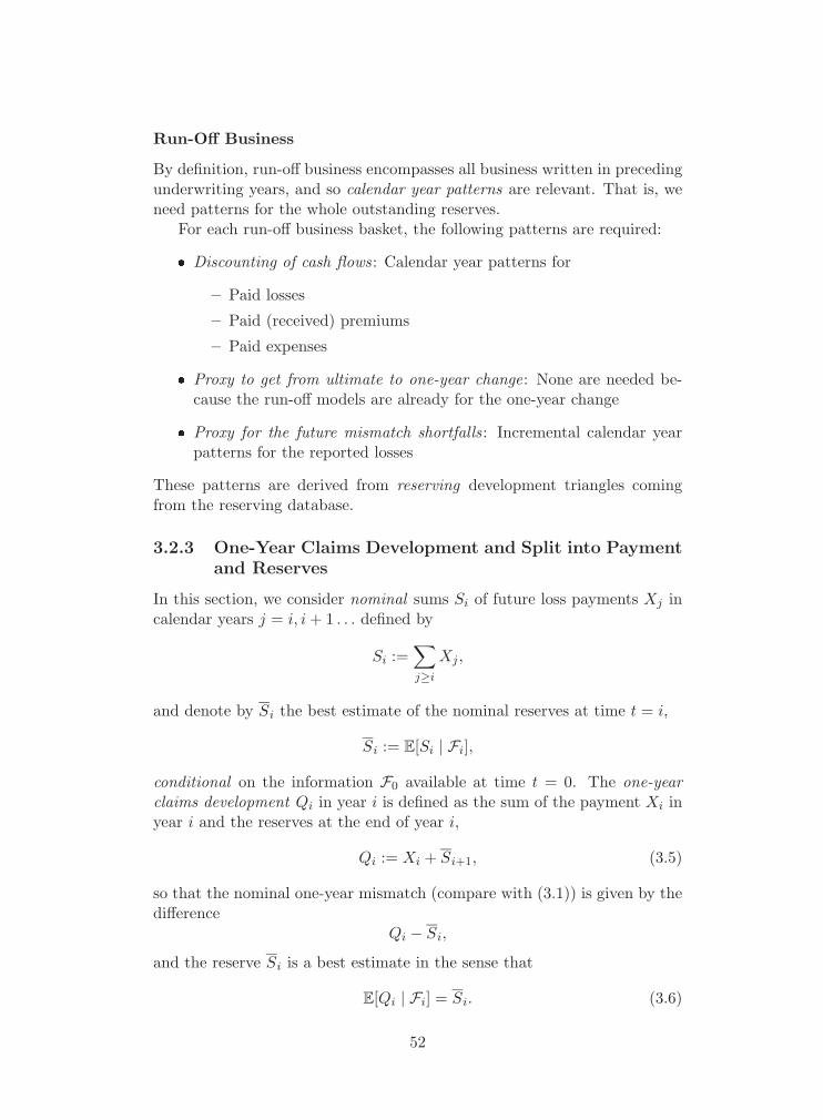
Run-Off Business
By definition, run-off business encompasses all business written in precedingunderwriting years, and so calendar year patterns are relevant. That is, weneed patterns for the whole outstanding reserves.
For each run-off business basket, the following patterns are required:
� Discounting of cash flows: Calendar year patterns for
– Paid losses
– Paid (received) premiums
– Paid expenses
� Proxy to get from ultimate to one-year change: None are needed be-cause the run-off models are already for the one-year change
� Proxy for the future mismatch shortfalls: Incremental calendar yearpatterns for the reported losses
These patterns are derived from reserving development triangles comingfrom the reserving database.
3.2.3 One-Year Claims Development and Split into Paymentand Reserves
In this section, we consider nominal sums Si of future loss payments Xj incalendar years j = i, i + 1 . . . defined by
Si :=∑j≥i
Xj ,
and denote by Si the best estimate of the nominal reserves at time t = i,
Si := E[Si | Fi],
conditional on the information F0 available at time t = 0. The one-yearclaims development Qi in year i is defined as the sum of the payment Xi inyear i and the reserves at the end of year i,
Qi := Xi + Si+1, (3.5)
so that the nominal one-year mismatch (compare with (3.1)) is given by thedifference
Qi − Si,
and the reserve Si is a best estimate in the sense that
E[Qi | Fi] = Si. (3.6)
52
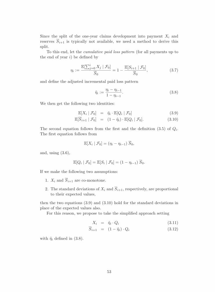
Since the split of the one-year claims development into payment Xi andreserves Si+1 is typically not available, we need a method to derive thissplit.
To this end, let the cumulative paid loss pattern (for all payments up tothe end of year i) be defined by
ηi :=E[∑i
j=0 Xj | F0]
S0
= 1 − E[Si+1 | F0]S0
, (3.7)
and define the adjusted incremental paid loss pattern
ηi :=ηi − ηi−1
1 − ηi−1. (3.8)
We then get the following two identities:
E[Xi | F0] = ηi · E[Qi | F0] (3.9)E[Si+1 | F0] = (1 − ηi) · E[Qi | F0]. (3.10)
The second equation follows from the first and the definition (3.5) of Qi.The first equation follows from
E[Xi | F0] = (ηi − ηi−1) S0,
and, using (3.6),
E[Qi | F0] = E[Si | F0] = (1 − ηi−1) S0.
If we make the following two assumptions:
1. Xi and Si+1 are co-monotone.
2. The standard deviations of Xi and Si+1, respectively, are proportionalto their expected values,
then the two equations (3.9) and (3.10) hold for the standard deviations inplace of the expected values also.
For this reason, we propose to take the simplified approach setting
Xi = ηi · Qi (3.11)Si+1 = (1 − ηi) · Qi (3.12)
with ηi defined in (3.8).
53

3.2.4 New Business, Prior-Year Business, and Run-OffBusiness Models
Recall from the introduction, pp. 41, the difference between earned andunearned business. We have defined unearned business at time t to bebusiness incepting before t for which we are still “under risk” at time t inthe sense that we might incur losses from loss producing events occurringafter time t. In the balance sheet, this distinction is reflected by providingthe “earned part” of the reserves only, and by accounting for the unearnedpart via the unearned premium reserves (UPR). With regards to unearnedpremium reserves, note that the SST considers an economic balance sheet,so the UPR have to be replaced by a best estimate of the correspondingliabilities.
As mentioned in the introduction, we make the simplifying assumption:
� Business written in a year i is fully earned at the end of year i + 1.
The distinction between earned and unearned business is relevant to usbecause we calculate the one-year mismatches Mi differently:
� For earned business, the mismatches are calculated using a “reservemodel” based on the reserving development triangles.
� For unearned business, we use a “new business model” based on pricingdistributions.
The reason for using the pricing distributions for unearned business is that,since this business is still “under risk”, catastrophic events might happenwhich result in an ultimate loss significantly different from the expectedoutcome. The corresponding volatility is captured in the pricing models bya strong focus on heavy-tailed distributions (see also Section 3.4, pp. 63).
As a consequence of having two different models for one-year mismatches,for instance at time t = 0, we would have to split the prior underwritingyear i = −1 business into an earned and into an unearned part and derivetwo different models, since not all of this business is fully earned at t = 0.
This issue is related to the actuarial estimation of the reserves. Stochasticmodels of the reserves are often based on the chain ladder method (see pp.93). However, in reality, the reserve calculation for the most recent yearsis typically not based on the chain ladder method, as that estimate is toouncertain. Instead, methods such as Bornhuetter-Ferguson are used, whichutilize models from pricing to a certain extent.
Our proposed approach takes both of these issues into account. Thebasic supposition is the following:
At time t = i,
54
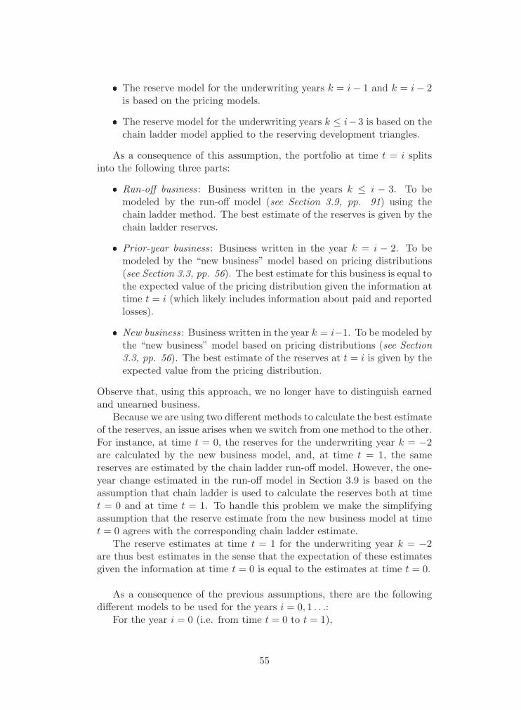
� The reserve model for the underwriting years k = i − 1 and k = i − 2is based on the pricing models.
� The reserve model for the underwriting years k ≤ i−3 is based on thechain ladder model applied to the reserving development triangles.
As a consequence of this assumption, the portfolio at time t = i splitsinto the following three parts:
� Run-off business: Business written in the years k ≤ i − 3. To bemodeled by the run-off model (see Section 3.9, pp. 91) using thechain ladder method. The best estimate of the reserves is given by thechain ladder reserves.
� Prior-year business: Business written in the year k = i − 2. To bemodeled by the “new business” model based on pricing distributions(see Section 3.3, pp. 56). The best estimate for this business is equal tothe expected value of the pricing distribution given the information attime t = i (which likely includes information about paid and reportedlosses).
� New business: Business written in the year k = i−1. To be modeled bythe “new business” model based on pricing distributions (see Section3.3, pp. 56). The best estimate of the reserves at t = i is given by theexpected value from the pricing distribution.
Observe that, using this approach, we no longer have to distinguish earnedand unearned business.
Because we are using two different methods to calculate the best estimateof the reserves, an issue arises when we switch from one method to the other.For instance, at time t = 0, the reserves for the underwriting year k = −2are calculated by the new business model, and, at time t = 1, the samereserves are estimated by the chain ladder run-off model. However, the one-year change estimated in the run-off model in Section 3.9 is based on theassumption that chain ladder is used to calculate the reserves both at timet = 0 and at time t = 1. To handle this problem we make the simplifyingassumption that the reserve estimate from the new business model at timet = 0 agrees with the corresponding chain ladder estimate.
The reserve estimates at time t = 1 for the underwriting year k = −2are thus best estimates in the sense that the expectation of these estimatesgiven the information at time t = 0 is equal to the estimates at time t = 0.
As a consequence of the previous assumptions, there are the followingdifferent models to be used for the years i = 0, 1 . . .:
For the year i = 0 (i.e. from time t = 0 to t = 1),
55

� Run-off business model for the underwriting years k ≤ −2 with initialamount at t = 0 from the actual balance sheet and one-year mismatchfrom the chain ladder run-off model.
� Prior-year business model for the underwriting year k = −1 withinitial amount from the balance sheet and one-year mismatch fromthe new business model.
� New business model for the underwriting year k = 0 with initialamount equal to the expected loss from the pricing model and one-yearmismatch from the new business model.
For the year i = 1,
� Run-off business model for the underwriting years k ≤ −1 with initialamount at t = 1 not needed and one-year mismatch from the chainladder run-off model2.
� Prior-year business model for the underwriting year k = 0 with initialamount not needed and one-year mismatch from the new businessmodel.
For the years i ≥ 2,
� Run-off business model for the underwriting years k ≤ 0 with initialamount not needed and one-year mismatch from the chain ladder run-off model.
3.3 Stochastic Model for New Business
In this section we describe the model for new business. By definition, thenew business N0 is the planned business to be written in year i = 0. Notethat a contract which is renewed in year i = 0 is considered new business,even though it is not, strictly speaking, “new” business in the sense that thiscontract has not been written in the prior year. The new business model isalso used for the pricing capital allocation (see Section 8.3, pp. 168 in thisdocument).
As outlined in Section 3.2, the new business portfolio N0 of business tobe written in year i = 0 is decomposed into baskets
N0 = N 10 ∪N 2
0 ∪ . . .
2The initial amounts at times t = 1, 2 . . . are not needed because the correspondingmodels are only used for the market value margin, and the calculation of the market valuemargin does not use the initial amounts but only the one-year mismatches.
56

with the dependency structure between baskets given by a portfolio depen-dency tree as described in Section 8.1. Note that, for ease of notation, wedenote here by M b
i the basket mismatches specifically for the new business.By definition, new business does not enter the calculation of the reserves
at t = 0 from (3.4), and it remains to calculate the basket mismatches
M bi = E[Rb
0 | Fi+1] − E[Rb0 | Fi] for i ≥ 0, (3.13)
conditional on the information available at time t = 0, and to specify theirdependency structure. See Section 3.3.2 (pp. 59) for the specification of thecurrent dependency structure.
Our approach to calculate the one-year basket mismatches M bi as de-
scribed in Section 3.3.3, pp. 62, is to scale the “ultimate change”
Rb0 − E[Rb
0 | F0]
by a factor 0 ≤ κbi ≤ 1 measuring the fraction of the ultimate change we
expect to be manifested in year i, i.e.
M bi = κb
i ·(Rb
0 − E[Rb0 | F0]
). (3.14)
The basket mismatches M bi according to Equation (3.14) are calculated
in three steps. First of all, using the pricing models, we obtain the distri-bution, conditional on the information available at t = 0, of the nominalultimate change
Sb0 − E[Sb
0 | F0], (3.15)
where Sbi for i ≥ 0 denotes the nominal sum of the future payments Xb
j ,
Sbi :=
∑j≥i
Xbj .
In a second step, the nominal sum Sb0 is discounted to get the difference
Rb0 − E[Rb
0 | F0].
Finally, this difference is transformed into one-year changes by (3.14).Considering the first step, the basket difference (3.15) is calculated by
two different approaches, see Section 3.3.2 (pp. 59).
� Default basket model : The model for a basket is constructed by ag-gregating the individual treaty pricing models of all contracts in thebasket priced in the pricing tool. Dependency between contracts isexpressed by an implicit dependency model using a multi-dimensionalcopula. The resulting figures are adjusted for contracts not priced inthe pricing tool. See Section 3.3.2 (pp. 59) for more on the defaultbasket model.
57
� Basket specific models: In these cases, the basket model is determineddirectly using an explicit dependency structure. As a general rule,specific models are used for business with a high impact on the balancesheet.
Because pricing models thus are part of the SST calculation, we provide anoverview of the pricing methodologies in Section 3.4, pp. 63. Note thatthe pricing models are for treaty business and not for facultative business.Facultative business is considered implicitly by adjusting the aggregatedpricing models to the planning figures, which include facultative business.We believe this approach to be justified as the current volume of facultativebusiness is small as compared to treaty business.
Considering the second step, to get discounted cash flows from nominalamounts, the cash flows are discounted using development patterns. Patternsexpress the expected cash flow in one year as a percentage of the nominalsum of all cash flows. More on patterns can be found in Section 3.2.2 (pp.50).
Concerning the third step, to transform the “ultimate change” to one-year changes by (3.14), see Section 3.3.3 (pp. 62).
3.3.1 Data Requirements and Parameters for New Business
We summarize the requirements on the SST new business model.
� Definition of the new business baskets (see Section 3.3.2, pp. 59)
� Treaty pricing models for the new business for a rolling year withinyears i = −1 and i = 0 including losses, premiums, expenses, as wellas development patterns (see Section 3.4, pp. 63).
� Planning figures for underwriting year i = 0 business, to calculategrowth factors for volume and inflation to adjust the pricing modelsto planned volume. Volume growth means growth in number of ac-counts, while inflation growth means growth in (average) treaty size,or inflation.
� Portfolio dependency tree to express the dependency structure betweenbaskets, including dependency parameters (see Section 3.3.2, pp. 59).
� Method (see Section 3.3.3, pp. 62) to transfer “ultimate changes”
Rb0 − E[Rb
0 | F0]
to one-year changes
M b0 = E[Rb
0 | F1] − E[Rb0 | F0]
� Development patterns: different types, see Section 3.2.2, pp. 50
58

3.3.2 Dependency Structure and Aggregation forNew Business
The dependency structure for new business is expressed by a portfolio de-pendency tree as described in Section 8.1 (pp. 148). The dependency treewe are currently using3 is shown in Tables 3.1, 3.2. Note that each basketneeds to be further split by legal entities.
Default Basket Model
In the default basket model, the basket distribution is derived by aggregationof the treaty pricing distributions. To express dependency between contractsin one basket, we use a multi-dimensional one-parametric Clayton copulawith parameter θ as described in Section 8.2.4.
Concerning the estimation of θ, we stress that we have by far insufficientdata to estimate θ statistically. We therefore rely on expert opinion to comeup with an estimate of the shifted lower tail dependency TD(q) as definedin 8.13 by expert opinion:
� Given that one contract in the basket at the end of next year is worsethan 1 in 100 years, what is the probability that any other contract inthe basket is worse than 1 in 100 years?
The treaty pricing models are then aggregated by drawing common sam-ples of the contract distributions using Monte Carlo methods. Note that thecontract losses, premiums, and expenses are co-monotone, so the same de-pendency assumptions can be used.
To reality-check the involved parameters derived by expert estimates, westudy
� Historical events which resulted in simultaneous claims in various linesof business
� The results of scenario evaluations
� The shape of the resulting aggregated basket models, to compare themwith historical basket outcomes and to “reality check” them by look-ing at different quantiles.
3The dependency tree is implemented with the proprietary aggregation tool Phobos.For a more detailed description of this IT system we refer to Part VIII of this documen-tation.
59

Property related (θ = 0.2260)
Agribusiness (θ = 0.2673)
Marine (θ = 0.3345)
Engineering (θ = 0.3350)
Property (θ = 0.0384)
Property Europe (θ = 0.1675)Property Europe NonCat (θ = 0.3350)Eurowind CatSouth Europe Cat
Property Japan (θ = 0.6206)Japan NonCat (θ = 0.7604)Japan Cat
Property rest of World (θ = 0.1607)RoW NonCat (θ = 0.1607)North America CatRoW Cat
Lloyds standard property (θ = 1.0227)
The property related baskets and the structure of the portfolio dependency treewhich are currently used and implemented in Phobos. For a basket, the θ valuein brackets specifies the multi-dimensional Clayton copula expressing dependencybetween the children of the basket. The two top baskets “Property related” and“Not property related” (see Table 3.2) are aggregated with θ = 0.1607.
Table 3.1: The portfolio dependency tree (property related baskets).
60
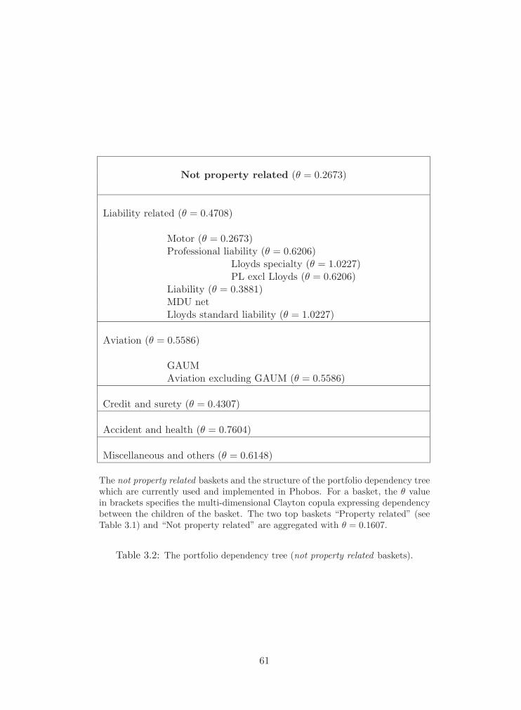
Not property related (θ = 0.2673)
Liability related (θ = 0.4708)
Motor (θ = 0.2673)Professional liability (θ = 0.6206)
Lloyds specialty (θ = 1.0227)PL excl Lloyds (θ = 0.6206)
Liability (θ = 0.3881)MDU netLloyds standard liability (θ = 1.0227)
Aviation (θ = 0.5586)
GAUMAviation excluding GAUM (θ = 0.5586)
Credit and surety (θ = 0.4307)
Accident and health (θ = 0.7604)
Miscellaneous and others (θ = 0.6148)
The not property related baskets and the structure of the portfolio dependency treewhich are currently used and implemented in Phobos. For a basket, the θ valuein brackets specifies the multi-dimensional Clayton copula expressing dependencybetween the children of the basket. The two top baskets “Property related” (seeTable 3.1) and “Not property related” are aggregated with θ = 0.1607.
Table 3.2: The portfolio dependency tree (not property related baskets).
61

Basket Specific Models
Basket specific models directly specify the basket distribution by an explicitdependency model. Currently, such basket specific models are available forProperty Nat Cat business (see Section 3.8, pp. 80), and for basket con-sisting of only one large individual contract (e.g. GAUM, MDU), where thebasket distribution is calculated directly by the responsible pricing actuary.Potential candidates for future specific models are Credit and Surety, andAviation.
Aggregation of Basket Models
Further aggregation of the baskets along the portfolio dependency tree fol-lows an approach analogous to the default basket model above, using amulti-dimensional Clayton copula.
3.3.3 One-Year Changes for New Business
In this section, we describe how to transform the “ultimate change” forbasket b,
Rb0 − E[Rb
0 | F0]
to the one-year change
M bi = E[Rb
0 | Fi+1] − E[Rb0 | Fi]
for i = 0. In general, the relation between the random variables of ultimateand one-year change would be given by a copula.
As an approximation, we use a linear proxy 0 ≤ κbi ≤ 1 to get from the
ultimate change to the one-year change, i.e.
M bi = κb
i ·(Rb
0 − E[Rb0 | F0]
). (3.16)
Since the one-year changes over all years i ≥ 0 should add up to the ulti-mate change, the sum of the κb
i for i ≥ 0 should be equal to 1. Moreover,κb
i should be largest for those years i where we expect the most significantchanges.
We propose to be consistent with the proposal of Section 2.2.3 (pp. 35)for the calculation of the market value margin, and thus to use as a proxyκb
i for the ratio of ultimate change to one-year change for new business fora basket the reported pattern by underwriting year for this basket:
� The proxy κbi for the ratio of one-year change in year i = 0 to ultimate
change for the new business from (3.16) is proposed to be the incre-mental underwriting year reported loss pattern for year i = 0, startingat January 1. Regarding patterns, see Section 3.2.2, pp. 50.
62

The rationale behind this approximation is that, for short-tail business, weexpect the biggest one-year change to occur in the first year i = 0, especiallywith regards to natural catastrophes (Nat Cat). The ultimate risk is thenvery close to the one-year change for year i = 0, and the correspondingpattern is almost at 100%.
For new long-tail business, the risk of a one-year change in year i = 0is small: It is very unlikely that new information for long-tail business willbe revealed during the first year, and this perception is confirmed by ourreserving data.
3.4 Treaty Pricing Models for New Business
As mentioned above, the SST model for new non-life business N0 written inyear i = 0 is based on treaty pricing models constructed by pricing actuar-ies and underwriters. Recall that new business here includes also renewedbusiness and not just business not previously written.
According to the pricing guidelines, all treaty business (with the excep-tion of very small treaties) has to be priced4.
The pricing workflow is set up in a way to guarantee that the treatyconditions assumed in pricing are consistent with the conditions specified inthe underwriting system5.
The pricing criteria specify which contracts have to be either priced by apricing actuary (or Nat Cat specialist), peer-reviewed by a pricing actuary,or which can be priced by an underwriter. Roughly speaking, the pricingcriteria for actuarial pricing/review apply to proportional bouquets withlarge premium (our share), and to XL programs with large limit and/orlarge premium (both for our share), with more restrictive criteria for thirdparty liability programs.
A similar set of peer review criteria specify which business has to bepeer-reviewed by a senior pricing actuary. Adherence to these criteria isregularly monitored in the pricing profitability study and audited by groupinternal audit. Current figures for underwriting year 2007 as per August 27,2007 show that 94.6% of the premium volume is priced in the pricing tool,and 84.5% of the premium volume is priced by pricing actuaries or Nat Catspecialists.
Roughly speaking, the general process for pricing a treaty consists of thefollowing steps:
1. Data requirements and analysis: Ensure that the data supplied by thecedent (i.e. the reinsured insurer) corresponds to the data require-ments for this particular type of business, and check whether the data
4In our proprietary pricing tool MARS. We refer to Part VIII.5The current underwriting system is GLOBUS.
63
is reasonable and, in particular, consistent with last year’s (and prioryear’s) renewal information.
2. “As if” adjustments to the data: The submitted data is usually his-torical or from a certain snapshot in time, so it has to be adjustedto the upcoming treaty period. Adjustments include rate changes,loss inflation, volume adjustments, changes in the underlying portfo-lio, development to ultimate amounts etc. One particular adjustmentis for incomplete years and/or incomplete most recent diagonal in adevelopment triangle.
3. Loss model fitting : In this step, one or several loss models are derivedfrom the adjusted data, typically by fitting a family of analytic distri-butions (e.g. log-normal, Pareto). Several loss models might be usedfor instance for different sub-lines of business covered. In particular,this step implies extrapolation of the available loss history to extremebad outcomes which have not yet been observed but can potentiallyoccur in the future. According to the pricing guidelines, at least onemodel has to use a heavy-tailed distribution. This is done to ensurethat extrapolation gives sufficient weight to catastrophic outcomes,and particular emphasis is put on the appropriate modeling of the tailof these distributions.
4. Stress Testing and Reality Checks: In this crucial step, the selectionof parameters underlying the loss model is varied to evaluate stabil-ity of the model and, if necessary, to refine it. Further, the resultingloss model is “reality-checked” by evaluating its reasonableness, for in-stance with regards to the past experience, the proposed reinsurancestructure, and information from similar types of treaties. Since theloss models are typically based on taking averages of adjusted histor-ical figures, it is crucial to check for trends remaining in the adjustedfigures. Existence of such trends typically suggest that the selectedadjustments do not fully capture changes to the business over time.There are various functionalities in the pricing tool available to assistthese enquiries.
5. Application of the treaty structure to the loss model : In this section,samples from the loss models are drawn by Monte Carlo simulation.In sampling, it is possible to consider dependencies between the dif-ferent loss models. Next, all relevant treaty and program features areapplied to the loss samples. This includes limits and deductibles, andloss dependent premium features (reinstatements etc.) and externalexpense features (sliding scale commission, profit commission, etc.).Features that apply on program level, i.e. to the aggregated outcomefrom several treaties, can also be considered. Then, the cash flows
64

are discounted using default or customized quarterly patterns. Theoutcome of these simulations is a distribution of the net present valueNPV of the contract result. This NPV distribution of the reinsuranceresults can be further “reality-checked.” See Section 3.4.5 (pp. 71) formore details.
6. Calculation of internal expenses and capital costs: This provides thefinal profitability estimate of the contract. The adequacy of the offeredconditions such as premiums is measured by the so-called performanceexcess (Section 8.3, pp. 168).
As a general rule, the loss model constructed in pricing is a stochastic modelof the nominal, ultimate losses to the cedent’s business subject to the reinsur-ance cover, in particular, prior to application of the reinsurance structure.Once such a “gross” loss model has been created, the specified reinsurancestructure is automatically applied to the loss model in the pricing tool, in-cluding discounting of the cash flows using default or customized patterns,and calculation of corresponding internal expenses and capital costs. (Re-garding patterns, see Section 3.2.2, pp. 50.) The calculation of the capitalcosts, the pricing capital allocation, is described in detail in Section 8.3 (pp.168).
Note that the pricing models are usually gross of retrocession. Retro-cession is only considered in pricing in case common account protection isin place for a specific program, so that the reinsurance premium can be re-duced by the costs of this retrocession, and the loss model can be adjustedfor the explicitly-given retrocession structure. Another potential situationcould be in case the cedent also purchases Fac reinsurance to the benefit ofthe reinsurance treaty under consideration.
For treaty pricing, we distinguish
� Proportional contracts (e.g. quota share, surplus)
� Non-proportional contracts (XL programs, stop-loss)
Pricing models can be based on
� Historical treaty results (experience pricing)
� (Estimated) exposure information (exposure pricing)
We describe proportional pricing in Section 3.4.1, and non-proportional pric-ing in Section 3.4.2. There is usually a default approach available, and theremight be specific approaches for certain lines of business. We consider allthese different approaches. More specific exposure pricing approaches aredescribed in specific sections for Property Nat Cat (Section 3.8, pp. 80),
65
Credit and Surety (Section 3.6, pp. 76), and Aviation business (Section3.5.1, pp. 75).
3.4.1 Proportional Pricing
Proportional business comprises Quota Shares, Surplus contracts etc. Char-acteristically, the sharing of premiums, losses and expenses between cedent(i.e. the insurer) and reinsurer is on a proportional basis.
From a modeling point of view, proportional business is distinguishedfrom non-proportional business in that, typically, any loss will impact thereinsurance treaty, whereas for non-proportional business, only sufficientlylarge losses need to be considered.
We therefore typically separately model the attritional or basic lossesand the large losses. Both attritional and large losses might be modeled byone or several different loss models.
� An attritional loss model is expressed by the aggregate distribution ofthe loss ratio without large losses and/or extremal events.
� A large-loss model is a frequency/severity model, where the frequencyis Poisson, Binomial, or Negative-Binomial distributed, and the sever-ities follow a heavy-tailed distribution such as Pareto or GeneralizedPareto.
The large-loss model is derived in the same way as the model for non-proportional treaties and is described in Section 3.4.2.
Attritional losses are losses which are observed regularly (“high fre-quency, low severity”), whereas large losses occur rarely, but have a highimpact on the result (“low frequency, high severity”). By creating a separatelarge-loss model, the tail of the loss distribution can be evaluated more pre-cisely. To a certain extent, the attritional loss amount is “more predictable,”and thus reflects the “quality” of the insured business, whereas large lossesreflect the “volatility,” i.e. the random component.
According to the guidelines, at least one loss model has to be heavy-tailed. Typically, the following rule is applied: If the large losses are mod-eled separately, the attritional losses are modeled by a log-normal or normaldistribution. In case no separate large-loss model is constructed (e.g. be-cause large-loss information cannot be obtained), the loss ratios are modeledby a Czeledin distribution. The Czeledin distribution is a log-normal dis-tribution up to a certain quantile, typically at 90%, and continued with aPareto distribution in the tail. In contrast to the log-normal distribution,the Czeledin distribution is heavy-tailed, and thus allows for considerationof the tail.
The model for the large losses is derived in the same way as for non-proportional treaties and is described in the next Section 3.4.2. It is based
66
on experience pricing or, preferably, on exposure pricing.
In the remainder of this section we thus describe the attritional lossmodel. It consists of the three steps data requirements, “as if” adjustments,and fitting an analytic distribution.
Data Requirements
The following data is required for the attritional loss model:
� Development triangles by treaty years and development years of theannual aggregate amounts of
– paid and outstanding or incurred (reported) losses
– earned premiums
� Estimated written premium for the upcoming treaty year
� Large-loss information
– ideally, with individual loss development
� Historical rate changes
� Information on the changes in the underlying portfolio/exposure overthe history period considered
“As-if” Adjustments
In order to model attritional losses only, the large losses need to be deductedfrom the loss triangle, to avoid double counting. Since large losses mightdistort the triangle development, it is preferable to remove the whole devel-opment of the large losses. In case this information is not available, it isassumed that the large losses are ultimate values, and their development isinferred from the triangle development to remove them.
The triangles need to be developed to ultimate amounts for each treatyyear. The default method used is the chain ladder method, but individualadjustments based on other methods are possible when appropriate.
One of the three assumptions of the Mack model for the chain laddermethod is that different treaty years are independent. From a theoreticalpoint of view, this implies that, before developing to ultimate amounts, thetriangles have to be “as if” adjusted to the level of the upcoming treatyperiod. Such adjustments include rate changes, loss inflation, changes inportfolio composition etc. The resulting adjusted estimated ultimate lossratios can then be interpreted as i.i.d. samples from one distribution, anddistribution fitting can be applied, see below.
67
An alternative approach is used, for instance, for Credit and Surety busi-ness. This method consists in estimating unadjusted ultimate historical lossratios by developing the unadjusted triangles. In many instances, the insur-ance cycle is visible in the time series of the unadjusted ultimate historicalloss ratios, once large losses are removed from the triangle. The expectedloss ratio for the upcoming treaty period can then be estimated by a naiveforecast of the insurance cycle, taking into account economic developmentsetc.
Regardless of the method used, it is always helpful to compare the finalloss ratio selection with the unadjusted historical loss ratios.
Fitting an Analytic Distribution
The families of analytic distributions available as a loss ratio model are thenormal, log-normal and Czeledin distribution. As mentioned above, theCzeledin distribution is usually used when no separate large-loss model isconstructed; otherwise, the other two options might be used.
In case the loss ratios are “as-if” adjusted as mentioned above, they canbe understood as i.i.d. samples from one distribution, and thus a directcurve fitting can be done: The distribution of loss ratio samples is fittedto an analytic distribution family (e.g. log-normal) by a chi-square methodtaking into account model uncertainty6. The fit is visualized graphically.
In case the loss ratios are not adjusted, such direct fitting is not possible,and we then use the following method: The expected loss ratio is estimatedas described above by naive forecast, and the standard deviation is estimatedfrom the annual changes in historical loss ratios.
3.4.2 Non-Proportional and Large-Loss Pricing Model
As mentioned before, loss modeling for non-proportional treaties and forthe large-loss model for proportional contracts is essentially the same, so wedescribe it at the same time. In both cases, the objective is to construct afrequency/severity model of losses exceeding a certain threshold.
There are two primary methods for constructing a large-loss model:
� Experience pricing, where the loss model is based on the historicallarge losses of the cedent
� Exposure pricing, which takes the actual exposures, i.e. the portfolioof risks, as a starting point
For experience pricing, two different methods are implemented in the pricingtool, one for short-tail and one for long-tail business. The two modules aredescribed in Section 3.4.3.
6The fitting method used is the same as the one used to fit severity distributions.
68
For exposure pricing, there is a standard method available based on theusual exposure curves. This method is described in Section 3.4.4.
Further, specific exposure models are used for
� Aviation, see Section 3.5, (pp. 74)
� Credit and Surety, see Section 3.6 (pp. 76)
� Property natural catastrophe business, see Section 3.8 (pp. 80)
3.4.3 Non-Proportional Experience Pricing
In the pricing tool, two different modules exist for experience pricing non-proportional contracts:
� Short-tail module
� Long-tail module.
The short-tail module is used for short-tail lines of business (e.g. Prop-erty non-cat, Marine); the underlying assumption in this module is that thenumber of historical losses and their severity do not have a large tail. Thelong-tail module is used for long-tail lines of business (Motor third party,liability etc.), where we expect further significant development for the pasttreaty years in the number of losses and in their size. In both modules, afrequency/severity model is constructed based on the historical losses of thecedent exceeding a certain reporting threshold.
To take into account changes in the portfolio over time, an exposuremeasure is required for the historical treaty periods, and an estimated figurefor the upcoming treaty period. The exposure measure selected is often therelevant premium (SUPI = subject premium income, or GNPI = gross netpremium income) received by the cedent for the reinsured business. Otherexposure measures are used when premiums are not an adequate measure.Examples for other exposure measures are total sum insured for Propertyper risk; number of vehicle years or number of insured policies for Motorliability; and class equivalents for doctors and bed counts for hospitals inmedical malpractice insurance etc.
If premiums are used as exposure measure, they must be developed toultimate amounts if necessary, and adjusted for rate changes to bring themto the current rate level. This requires information on historical and plannedrate changes. If available, premiums should be further adjusted for changesin the underlying risk and insurance coverage, such as changes in deductiblesand limits.
69

Historical losses are “as if” adjusted to the level of the upcoming treatyperiod, taking into account loss inflation, potential loss caps etc. Stabi-lization clauses (index clauses) are applied to the layer if applicable. Theythen have to be developed to ultimate values if applicable. In the long-tailmodule, this development does not apply to individual losses but to the ag-gregate losses to a suitably selected layer, both in a triangle of the aggregateloss to layer and in a triangle of the number of losses to layer. To developthe triangle, chain ladder and cape cod methods are available.
Finally, the losses are adjusted for changes in the exposure measure, ei-ther by adjusting their frequency (“per risk”), or by adjusting their severity(“per event”), to take into account changes in the portfolio over time.
In the short-tail module, the expected frequency of losses exceeding aselected model threshold is calculated as a weighted average of the adjustednumber of losses. This determines a Poisson distribution for the numberof losses. By considering the Q-Panjer factor (the standard deviation di-vided by the expected value), it can be evaluated whether Poisson is a goodmodel. Alternatively, a Binomial or Negative-Binomial distribution can bedetermined. The severity distribution is determined by fitting an analyticdistribution to the adjusted losses exceeding the threshold by a chi-squaremethod. Severity distributions used are heavy-tailed and typically Pareto,Generalized Pareto, or log-gamma. In particular, this leads to an extrapola-tion of the observed losses to higher loss amounts.
In the long-tail module, the expected frequency to calibrate a Poissondistribution is derived from the development of the triangle of the number oflosses to layer. For the severity, a Pareto distribution is calculated from theexpected frequency and the expected loss to layer (“burning cost”) obtainedfrom the developed triangle of total loss to layer.
The pricing tool offers a number of visual helps to determine the goodnessfit of the model to the data, the adequacy of projections to higher layers,and the detection of trends.
3.4.4 Standard Exposure Pricing
Standard exposure pricing is based on the risk profile of the cedent or, moregenerally, on the portfolio of insured risks. The risk profile combines therisks into sum insured bands (or limit bands for liability business): All riskswhose sum insured is between minimum and maximum of a given band areassigned to this band.
The information required per band consists of
� The number of risks in the band
� The average sum insured of these risks
70

� Their total premium
The pricing tool is also able to handle layered profiles, i.e. profiles of layers.To derive a frequency/severity distribution from the risk profile, one has
to select an exposure curve and estimate an expected loss ratio per band.Given a risk profile, the risks in a band are automatically distributed
within the band consistent with the average sum insured per band. Fromthe exposure curve, the severity distribution of each risk is derived, seebelow. From the expected loss ratio and the total premium, the expectedloss per band is derived, which in turn allows to calculate the expected lossfrequency per band. The resulting individual model is approximated by acollective model in the form of a compound Poisson model, providing thedesired frequency/severity model.
The exposure curves used for Property business and other lines are so-called deductible Rebate curves. These curves correspond to the loss degreedistribution, that is, the distribution of the severity as a percentage of thesum insured. The underlying assumption when applying a Rebate curve toa portfolio of risks with different sums insured is that the distribution of theloss degrees is the same for all risks in the portfolio; in particular, the lossdegree is assumed to be independent of the sum insured. Since this is notalways correct (e.g. Property per risk), different curves might need to beapplied to different bands.
For other types of business, primarily for third party liability business,other types of exposure curves are selected, such as increased limit factor(ILF) curves. The assumption underlying this model is that the absoluteseverity distribution is the same for all risks in the band, but that the severityis capped at the appropriate risk limit.
In the pricing tool, the risk profile can be adjusted in various ways (vol-ume changes, inflation, inuring quota share or surplus); and a variety ofexposure curves are available (Swiss Re Y-curves, MBBEFD, ISO, Riebe-sell, ILF, user-defined curves).
3.4.5 Calculating the Treaty NPV Distribution
In this section, we describe the derivation of the treaty NPV (net presentvalue) distribution of the treaty results, i.e. the distribution of the presentvalue of
premium − losses − external expenses − internal expenses.
In view of the preceding sections, we have available one or several stochas-tic loss models of the cedent’s business subject to the reinsurance cover.Typically, these models provide the nominal ultimate losses. The task isthen to apply all relevant reinsurance treaty and program features to theseloss models, and to discount the cash flows.
71

In general, the structure of a reinsurance deal is given by a program con-sisting of one or several treaties. For instance, a non-proportional programmight consist of different layers, and a proportional bouquet of several quotashares. Moreover, certain programs might consist of both proportional andnon-proportional treaties. An example is given by a quota share treaty to-gether with one or several XL layers on the retention of the quota share.Because a sufficiently large loss will affect both the quota share and theXL layers, it is crucial to model the two treaties together. More generally,profitability of a deal has to be evaluated on the program level. All struc-tures mentioned above can be captured in our pricing tool; in particular,proportional and non-proportional treaties can be considered together.
To calculate the reinsurance result, a number of different loss modelsderived for the reinsurance program (as described in the previous sections)are available. The following types of loss models can be considered:
� Aggregate distributions, either as loss ratios or as absolute loss amounts,for the distribution families Normal, Log-Normal, Czeledin, Empiric(piecewise linear), and Discrete (step function).
� Frequency/severity distributions with frequency distribution familiesof Poisson, Binomial, Negative Binomial, Panjer, and Bernoulli; andas severity distributions, Log Normal, Czeledin, Pareto, GeneralizedPareto, Gamma, Log Gamma, Empiric, Discrete.
� Cat : Event loss tables for major perils used to model natural catas-trophe risks
� Aviation specific loss model for the Aviation market model.
The appropriate loss models are attached to the treaties in the program.Several treaties can use the same loss model, and several loss models can beused for one treaty.
The NPV distribution is determined by Monte Carlo simulation. Thenumber of simulations can be selected manually and is typically around1′000′000 iterations. The whole calculation for such a case usually takesa few seconds. The NPV distribution is determined in the following threesteps applied for each individual simulation iteration:
� For each loss model, a loss sample is drawn. Dependencies betweendifferent loss models can be considered, if appropriate, by means ofa multidimensional Clayton copula (see Section 161, pp. 161). Thismay enable more appropriate modeling of the tail.
� The quarterly cash flows of the (ultimate) loss samples are derivedusing quarterly patterns for premiums and losses, either using defaultpatterns or patterns derived from cedent data.
72

� The relevant terms and conditions are applied to the loss cash flows toderive cash flows for losses after reinsurance, premiums, and expenses.A list of terms and conditions considered is found below. In this step,rational cedent behavior is taken into account, for instance for the caseof a no claims bonus (NCB).
� Next, the derived cash flows are discounted to obtain the present valueat treaty inception. This is done by selecting for each cash flow theyield for the appropriate maturity from default yield curves in theappropriate currency from Bloomberg (for government bonds in therespective currency).
After completion of all simulation iterations, internal administrative ex-penses, the NPV distribution, and the allocated capital costs are calculated.Profitability of the program is measured by the performance excess (see Sec-tion 8.3, pp. 168).
The relevant terms and conditions are usually imported from the un-derwriting administration system. The pricing tool supports treaty featuressuch as
� Limits, retentions, AAD (annual aggregate deductibles), AAL (annualaggregate limits)
� Premium features, including reinstatements and swing rates
� External expense features such as fixed or sliding commissions, bro-kerage and other expenses, fixed or sliding profit commissions
� NCB (no claims bonus), common account protections, loss corridors
� Etc.
as well as aggregate features over several contracts in one program:
� AAD, AAL, NCB
� Profit commission (fixed or sliding), sliding scale commission.
In order to analyze the program results, simulation results are availablefor the whole program as well as for each treaty. They include
� Expected values and standard deviation for premium, loss, expenses,and NPV
� Expected cash flow effect to measure the impact of discounting of cashflows on the result, and on premiums and losses
� Graphs of the cumulative distribution function for losses, premiums,expenses, and NPV
73
� Measures of profitability such as performance excess, TRAC (time andrisk adjusted capital, see Section 8.3, pp. 168), (stand-alone) expectedshortfall of the NPV
� Risk transfer checks to ensure that the program fulfills risk transfercriteria
� Above figures allow plausibility checks such as
– expected shortfall of NPV / expected premium (“how many timesthe premium is lost in a very bad outcome”)
– performance excess / TRAC (“excess return on capital”)
– probability of negative NPV (“probability that we lose money”)
and further figures to allow checks for non-proportional business,
– probability of loss > 0 (“probability of loss to layer”)
– probability of aggregate loss > 0 (“probability that one limitstretch is not sufficient”)
– probability of maximum aggregate loss (“probability of using upthe whole capacity, including reinstatements”).
Once the final pricing version of a program is determined, the corre-sponding treaty results are transferred to the underwriting adminstrationsystem.
3.5 Exposure Pricing for Aviation
In the following we outline the exposure pricing approach for Aviation busi-ness. Experience pricing is normally not used because there is in generalnot enough loss experience to model large losses based on the client’s lossexperience alone.
General aviation business is priced with the standard exposure pricingapproach. Specific market exposure curves of the distribution of the loss aspercentage of sums insured are available. The exposure information consistsof client risk profiles by type of coverage (e.g. Hull, Liability) with numberof policies, sums insured, and premiums per band.
For direct airline business a specific exposure pricing approach is used.The exposure information needed here is the standardized aviation ques-tionnaire providing, in particular, detailed information about the client’sexposures on individual airlines/manufacturers (Non-US Airlines, US Air-lines, Products). Our standard approach is to use our in-house aviationmarket model to simulate market losses, and to apply to these market lossesthe client’s market shares from the questionnaire information. The aviationmarket model is described in more detail in the next section.
74
3.5.1 Aviation Market Model
Our aviation market model developed in-house applies for direct airline busi-ness. We simulate market losses for Non-US Airlines, US Airlines and Prod-ucts and apply the client’s shares to these simulated market losses. Themodel simulates market losses in excess of USD 100 million. For both Non-US Airlines and US Airlines, we simulate a random number of losses, corre-sponding severities, and the primary policies affected by the losses. Further-more, with certain probabilities, related manufacturer’s losses are simulatedand added to the pure Airline losses. Pure Product losses are simulatedin addition. For each of the losses it is simulated if other airlines or man-ufacturers are involved (multi-losses). If yes, additional loss severities aresimulated the same way.
Underlying Data
Our market model is based on historic market losses. The indexed marketlosses are analyzed in our pricing tool and fitted to heavy-tailed severity dis-tributions. As exposure measures the market premiums are used, adjustedfor market rate changes. Frequencies are simulated with a Negative Bino-mial distribution. The market premium and premium rate changes for Hull,Liability and Products come from different sources/brokers.
Application
We are mainly interested in the schedule A (Non-US Airlines), B (US Air-lines) and C (Products) of the standardized aviation questionnaire, giv-ing detailed information about the airlines/manufacturers exposures of theclient.
We assume a market loss hits always a questionnaire listed airline (Non-US Airline, US Airline) or questionnaire listed manufacturer (Products).Please note that not all airlines are part of the questionnaire. Therefore onebasic assumption is that the questionnaire is a representative sample, i.e.we assume the same behavior for non-listed airlines/manufacturers. Eachairline respectively manufacturer has a certain probability assigned to be hit.This specific probability is calculated based on various exposure measures.
One major issue simulating market losses is that not each market losscan be a loss for each of the airlines respectively manufacturers, due to thegiven policy limit, in particular the very high market losses. Therefore onehas to calculate the conditional probabilities that a specific airline or manu-facturer has caused a given market loss. Based on the given policy limits wecreate baskets of all possible market losses with probabilities and possibly
75
affected airlines respectively manufacturers. In these baskets we calculatethe conditional probabilities of these airlines respectively manufacturers.
Having simulated these market losses and allocated to the airlines respec-tively manufacturers in the way described above, the individual client shareson these losses can be calculated, based on the questionnaire information wereceived.
3.6 Credit and Surety Exposure Pricing
We outline here the standard exposure pricing approach for credit and bondbusiness. Political risk and US Surety are excluded in this part.
The methodology is outlined by Bea Wollenmann, Standard Approach toPricing Credit and Bond Reinsurance Treaties (Wollenmann [2007]). Thefollowing sections reproduce this paper.
3.6.1 Data Requirements
For any type of reinsurance treaty covering trade credit or bond, the list ofgranted credit limit per risk and bonded limits per risk for “major” risks isindispensable. As exposure one uses for credit risks the granted limit, i.e.the limit of insured credits per risk set by the insurer, and the bonded limitper risk for bond exposures. The notion of granted limit must be consistentwith the one agreed upon in the PML-study (Stahel and Jaggi [2003]). Forproportional covers, we call a risk major, if the exposure to the treaty (=sumof the covered limits) is greater than 5% of the cedent’s GNPI. In case of anXL-cover, a risk is major if the exposure is greater than the priority of thesmallest layer. Depending on inflation and expected growth, also risks whichare currently not exposing the XL-programme might do so in the course ofthe contract period and need therefore be considered accordingly in pricing.
The cedent should report his internal ratings for all major risks as well.Moreover, a risk profile for non-major risk is highly desirable. Anticipatedshifts in the risk profile between the reported profile and the expected profileduring the covering period need to be reported as well.
In case of bond coverage on a risk attaching basis, a split by underwritingyear is needed. However, there are so far only few cedents reporting on thatbasis. Ideally, the cedent’s report is split by types of bonds as well.
3.6.2 Loss Model
For an exposure-based loss modeling we use in principle the individual modeland the corresponding collective model obtained by compound Poisson ap-proximation (see Rolski et al. [1999]). To this end, a probability of defaultand a loss-given-default-distribution (LGD-distribution) is associated witheach risk.
76

The probability of default for a single risk is generally obtained fromMoody’s KMV. In case the risk can be found in MKMV, then we use the1-year EDF (Expected Default Frequency) for the company. In case a risk isnot monitored in MKMV (e.g. non-public companies) or in case the modelis based on a profile with unnamed risks in each band, then we select anappropriate EDF. To this end there are various approaches from which weselect the one which seems most appropriate:
1. Mapping cedent’s internal ratings with EDF for those risks which arecovered by MKMV using a regression analysis.
2. Taking average EDFs over an appropriate universe, e.g.
(a) The intersection of cedent’s portfolio with the risks covered byMKMV.
(b) Depending on the quality of the portfolio, select an EDF betweenthe median and the 10% quantile of MKMV’s EDFs for countryor industry sector.
(c) Individually assessing a risk by comparing it with its peers inMKMV.
It remains to choose the appropriate LGD-distribution which is equivalent tochoosing an exposure curve. There are essentially three cases to distinguish:
1. Trade credit exposure: We choose the LGD-distribution from the PML-study and distinguish between large and small insurers.
2. Bond exposure: This depends very much on the type of bond. Ifthe cedent provides sufficient data of his historic losses, then we canconstruct an individual LGD distribution. Otherwise, we have histor-ical data from a large European cedent which allowed us to deducea rough LGD-distribution and which we used for similar business ofother clients in Europe as well. Another approach is the selection of
7 In general, E(LGD) should not be smaller than35%.
3. Mixture of bond and trade credit exposure: We build a mixture ofthe corresponding LGD-curves for credit and bond. The mixture isdone under the assumption of co-monotonicity between credit- andbond-LGD. Usually it suffices to split the portfolio into not more thanfive risk groups, namely a group with a negligible, small, medium,high bond exposure and a group with negligible credit exposure. Themixture of the LGD-curves is done for each group based on its averagecredit-bond-mix.
7MBBDEF stands for Maxwell- Boltzmann, Bose- Einstein, Fermi- Dirac, three classesof analytical exposure curves derived from (and named after) the three major sorts ofprobability distributions used in statistical mechanics.
77
Note that for the exposure loss model we do not make use of the actualpremium per risk. Instead, we calculate for each risk its EDF multiplied withits limit and the expected loss given default. This calculated figure is usedin the exposure model as premium and equals the expected ground-up lossof the considered risk. In the usual exposure module, an implicit probabilityof loss is calculated from the premium and loss ratio information and theselected exposure curve. If we enter for the premium the figure describedbefore and set the loss ratio to 100%, then the implicit probability of loss,deduced from this input, is again the EDF of the considered risk.
3.7 Credit and Surety Outlook: Portfolio Model
3.7.1 Modeling Approach
We receive from our clients sufficient information that it would in principlebe possible to model the tail of the loss distribution for our whole creditand bond portfolio, and gain also explicitly the tail dependency between anindividual contract and this total credit and bond portfolio.
To reach this goal, we would need to do a Monte Carlo simulation, se-lecting in each iteration the companies defaulting randomly but with theprobability given by their EDFs. The loss given default could be selected co-monotone from the different LGD distributions for all contracts exposed tothis specific defaulting risk. Finally, applying all contracts to the simulatedlosses exposing them in one iteration, we could obtain our loss distributioncoming from these largest exposures and also measure the tail dependencybetween any two contracts or a contract and the rest of the portfolio.
However, if one looks closer to the details, there are several problems tobe overcome to complete this task. While we have already resolved some ofthem and have set up our internal tools, especially also our accumulationcontrol CrediEx, such that they will support such an approach, it would stillbe a major project to reach this goal.
3.7.2 Identification of the Risks
The risks for credit and bond are the individual companies. However, thereis usually not a unique standard name for a specific company, but eachcedent might spell its name in a slightly different way. Furthermore thereare often highly complex legal and economic structures between holdingsand their subsidiaries, and these structures change dynamically over time.
While we do not have the resources to model these complicated relationsexactly, we nevertheless have built up a database supporting an adaptive,semiautomatic mapping between the different spellings of a company and itsunique, internally standardized name, which is the name used in MKMV if
78

available. Additionally, in this database we can also define simple hierarchi-cal structures over several levels of holdings, the subsidiaries they control,and the subsidiaries of the subsidiaries. This database, which is an integralpart of our accumulation control system CrediEx, allows therefore a fastidentification of the risks reported by the cedents and the accumulation ofour exposures on the holding level.
3.7.3 Estimation of the True Exposure per Risk
In order to do a simulation as outlined in Section 3.7.1, we need for eachcontract of the considered portfolio and each risk exposing this contractinformation on the ground-up exposure, the EDF and the LGD distributionof this risk. While the EDF is a fixed number for each risk, the ground-upexposure and the LGD distribution depend on the contract and the type ofcredit or bond exposure. It is not straightforward how to set these figuresand distributions.
� Exposures: Often the cedents report us their current limits per riskonly on an accounting year basis, while the reinsurance contract workson a risk attaching basis. Therefore, taking the figures as given bythe cedent would lead to an overestimation of our exposure from thiscontract in the first year and an underestimation in the subsequentyears. We resolved this problem in CrediEx by estimating typicalpatterns for the average duration of different types of bonds. Thisallows us to have a more adequate estimate of our exposures fromsuch contracts until the bonds mature.
� EDF: If a company can be found in MKMV, then we have its EDFavailable in CrediEx. For all other companies the way how to assignthem an EDF would need to be defined. It could depend on EDFquantiles in MKMV for the country or the industry segment of thecompany or on the internal ratings of the company from some of ourcedents.
� LGD: Except for pure trade credit there are so far no standard LGDdistributions which could be applied directly, so they would need tobe defined first. Then we would need to extend the functionality ofCrediEx to assign them to the different types of bonds. If the exposureon a company comes from several types of bonds with different times tomaturity, then the combined LGD distribution would need to changeover time accordingly. This is not yet implemented in CrediEx, butis feasible since this tool has been designed already in view of suchpossible extensions.
79

3.7.4 Simulation
Currently it is not possible to run simulations in CrediEx, but would requirea further extension of the functionality of this tool. A simulation for thewhole credit and bond portfolio would require many iterations in order to getan adequate loss distribution also in its tail. Therefore efficient calculationswould be key in order to run such a simulation within reasonable time.
Furthermore, one could also think of modeling dependencies betweenthe defaults of different companies and/or the severity of their losses, or toinclude economic scenarios in the model.
3.8 Natural Catastrophe Modeling
SCOR Switzerland’s natural catastrophe modeling is described in the paperby Brigitte Pabst, Flavio Matter, Natural Catastrophe Modeling (Pabst andMatter [2008]). The following sections of our documentation are based onthat paper.
3.8.1 General Approach
The analysis of SCOR Switzerland’s natural catastrophe (NatCat) exposurefor property lines of business is primarily performed with NatCat modelingsoftware that is widely accepted in the insurance market. The basic conceptof modeling is very similar in all catastrophe models. The following sectionprovides an overview on:
� Framework of probabilistic cat models
� Sources of uncertainty
� Sensitivity of model parameters and
� Clash potentials
The probabilistic approach comprises modules (Figure 3.1), which ac-count for hazard, exposure, vulnerability and financial conditions to esti-mate insured losses.
The hazard is defined by a simulated set of events. This simulated eventset is developed based on a statistical parametric approach or a numericalsimulation. The common statistical approach derives the hazard informa-tion mainly from a historic event catalog that covers the range of observedevents with respect to size, location and probability of occurrence. Themore complex numerical models simulate time-dependent, three-dimensionalstructures. The potential impact of the hazard at each location is translatedinto damage through so-called vulnerability functions. Those sets of rela-tionships describe the degree of loss to a structure resulting from exposure
80
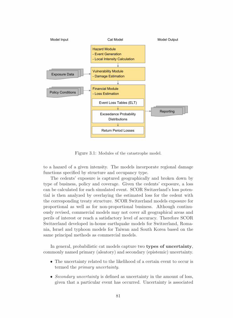
Financial Module- Loss Estimation
Exposure Data
Hazard Module- Event Generation- Local Intensity Calculation
Vulnerability Module- Damage Estimation
Policy Conditions
Model Input Cat Model Model Output
Reporting
Event Loss Tables (ELT)
Exceedance ProbabilityDistributions
Return Period Losses
Figure 3.1: Modules of the catastrophe model.
to a hazard of a given intensity. The models incorporate regional damagefunctions specified by structure and occupancy type.
The cedents’ exposure is captured geographically and broken down bytype of business, policy and coverage. Given the cedents’ exposure, a losscan be calculated for each simulated event. SCOR Switzerland’s loss poten-tial is then analyzed by overlaying the estimated loss for the cedent withthe corresponding treaty structure. SCOR Switzerland models exposure forproportional as well as for non-proportional business. Although continu-ously revised, commercial models may not cover all geographical areas andperils of interest or reach a satisfactory level of accuracy. Therefore SCORSwitzerland developed in-house earthquake models for Switzerland, Roma-nia, Israel and typhoon models for Taiwan and South Korea based on thesame principal methods as commercial models.
In general, probabilistic cat models capture two types of uncertainty,commonly named primary (aleatory) and secondary (epistemic) uncertainty.
� The uncertainty related to the likelihood of a certain event to occur istermed the primary uncertainty.
� Secondary uncertainty is defined as uncertainty in the amount of loss,given that a particular event has occurred. Uncertainty is associated
81
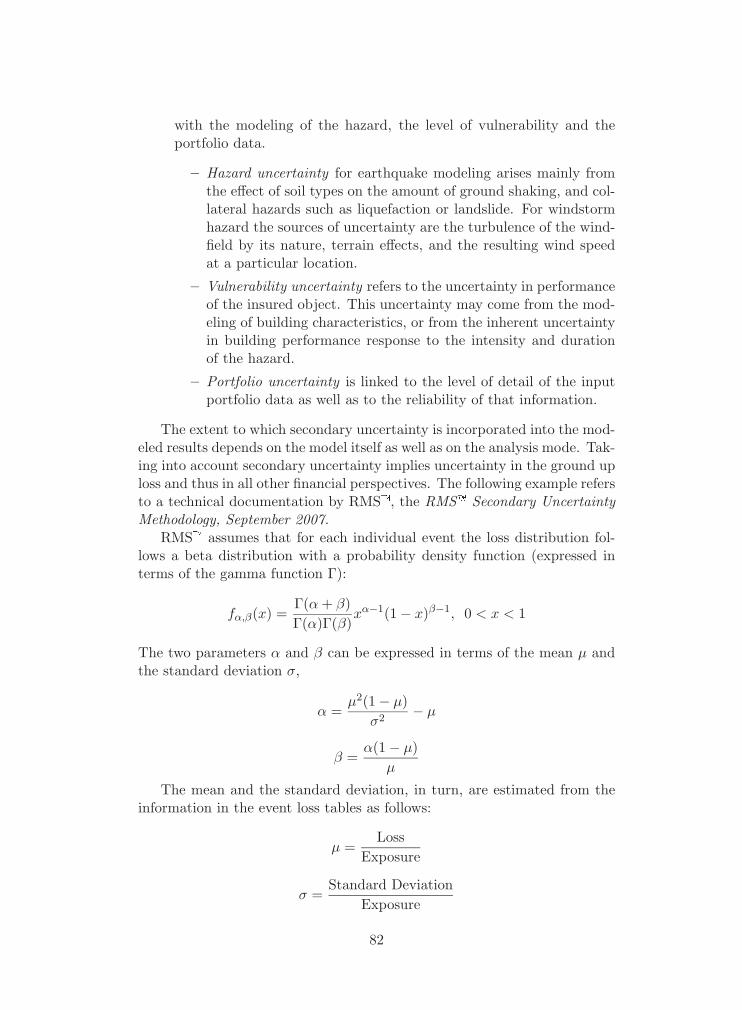
with the modeling of the hazard, the level of vulnerability and theportfolio data.
– Hazard uncertainty for earthquake modeling arises mainly fromthe effect of soil types on the amount of ground shaking, and col-lateral hazards such as liquefaction or landslide. For windstormhazard the sources of uncertainty are the turbulence of the wind-field by its nature, terrain effects, and the resulting wind speedat a particular location.
– Vulnerability uncertainty refers to the uncertainty in performanceof the insured object. This uncertainty may come from the mod-eling of building characteristics, or from the inherent uncertaintyin building performance response to the intensity and durationof the hazard.
– Portfolio uncertainty is linked to the level of detail of the inputportfolio data as well as to the reliability of that information.
The extent to which secondary uncertainty is incorporated into the mod-eled results depends on the model itself as well as on the analysis mode. Tak-ing into account secondary uncertainty implies uncertainty in the ground uploss and thus in all other financial perspectives. The following example refersto a technical documentation by RMS�, the RMS� Secondary UncertaintyMethodology, September 2007.
RMS� assumes that for each individual event the loss distribution fol-lows a beta distribution with a probability density function (expressed interms of the gamma function Γ):
fα,β(x) =Γ(α + β)Γ(α)Γ(β)
xα−1(1 − x)β−1, 0 < x < 1
The two parameters α and β can be expressed in terms of the mean μ andthe standard deviation σ,
α =μ2(1 − μ)
σ2− μ
β =α(1 − μ)
μ
The mean and the standard deviation, in turn, are estimated from theinformation in the event loss tables as follows:
μ =Loss
Exposure
σ =Standard Deviation
Exposure
82

For detailed loss modeling (RiskLink DLM Japan) the basic input to thefinancial module is the individual location coverage value, the event groundup mean damage ratio and associated coefficient of variation. The meandamage ratio defines the percentage of total exposed value damaged in anevent at the specific location coverage. The mean loss as a ratio to the expo-sure commonly refers to as the mean damage ratio (MDR). The secondaryuncertainty in the size of loss is represented by the coefficient of variation,which equals the ratio of the standard deviation to the mean. The portfoliostatistics are then built up from the location coverage statistics, event byevent. The estimated probability distribution of damage at each locationmust then be combined with the distributions from all other locations. Thisis accomplished through a convolution process.
For calculations on the aggregated exposure (RiskLink ALM, Catrader)level, the concept is to match aggregate exposures with a precompiled data-base of loss ratios and associated coefficients of variation. This is done fordifferent lines of business at predetermined aggregate geo-code levels. Thestandard deviation therefore is based on an industry average precompiledat an aggregate level, and not calculated directly from individual locationsand summed as is done in detailed loss modeling.
A sound understanding of the uncertainties associated with the model’skey parameters is essential for the interpretation of the model outcome andthus for decision making. The model outcome describes a bandwidth of lossestimates and not a unique value. In order to identify and stress-test the keyparameters, systematic sensitivity analyzes have to be conducted for eachmodel release.
Another issue for cat modeling is the treatment of clash potentials ofneighboring geographical zones, of perils or treaties. SCOR Switzerland hasadopted a central monitoring system8 to manage the worldwide accumu-lations of catastrophe risk by peril and region. The accumulation controlfocuses on zones with a geographic concentration or peak exposures, such asUS hurricane risk. This centralized analysis is essential for a global reinsurer,since business is written for the same region from more than one worldwideoffice. Great efforts were also undertaken to monitor clash potential, bothfrom lines other than property catastrophe.
8Global Cat Data Platform, GCDP, see Part VIII
83

3.8.2 Hazard Module
Wind
Windstorm modeling differs between atmospheric phenomena. The mostrelevant perils producing insurance losses are tropical cyclone, extratropicalcyclone, tornado and hail.
Tropical cyclones, regionally also called hurricanes or typhoons, formand spend much of their life cycle in the tropical latitudes, which are char-acterized by large areas of relatively uniform pressure. Tropical cyclonestend to be structured, self-contained systems. These characteristics makethe parameterized modeling approach an appropriate one. In modeling trop-ical cyclones, the most relevant parameters are central barometric pressure,radius of maximum windfield, and forward speed. Central pressure is theprimary determinant of a tropical cyclone’s wind speed and, therefore, ofits intensity. Minimum central pressure is the lowest sea level pressure mea-sured at the centre of the tropical cyclone. Wind speed can be describedas a function of pressure differential between the central pressure and thepressure outside the storm centre. For each of these model variables, themodeler fits theoretical probability distributions to the historical data, test-ing the goodness-of-fit.
A common approach for modeling the range of potential tropical cy-clones is based on a set of stochastic storm tracks. This stochastic eventset enables reliable estimation of events with large recurrence rates andfor all geographical areas. This event catalog contains the pre-simulatedphysical parameters, location, and frequency for each storm. Under cer-tain conditions, storms may transform into extra-tropical storms. Knownas transitioning storms, these tropical systems interact with the jet streamand become more asymmetric with time. The strongest winds push to theright-hand side of the storm over a broader region than one finds in a hur-ricane. All such parameters have to be taken into account while generatingthe stochastic event set. A common approach is the generation of the eventset with the help of a Monte Carlo algorithm simulating the random behav-ior of each single storm system. The stochastic-generated event set is thencalibrated against historical track data.
While running an analysis the hazard module determines the peak-gustwind speed at each property location for every stochastic event that is likelyto cause loss at that location. Beside the wind speed itself, another damage-causing component of hurricanes is surge. Most models include the optionto model the height of surge for each stochastic storm and analyzed loca-tion. The impact of topography for both phenomena, wind speed and stormsurge, is considered through surface roughness factors and a digital height
84
model.
Extratropical cyclones, such as European windstorms, are more com-plex than tropical cyclones. Atmospheric conditions in the mid-latitudescontain multiple high-pressure ridges, low-pressure troughs, fronts, and strongjet stream winds all interacting to develop complex storm systems. Whilea parameterized approach to modeling storm tracks works well for the rel-atively simple and symmetric horizontal structure of tropical cyclones, theapproach falls short when it comes to modeling extratropical cyclones.
An alternative to the approach of predefined storm tracks offer numeri-cal weather prediction models. Those use global environmental data such assea surface temperatures, wind speed and pressure in conjunction with thephysical equations that govern the atmosphere. Beginning with an initialsnapshot of conditions at the surface and multiple upper atmospheric lay-ers, the dynamic three-dimensional wind-field is derived from a set of partialdifferential equations governing fluid flow. Topographic effects such as ridg-ing, sheltering and channeling are captured by gridded elevation and landuse information. Depending on the spatial and temporal resolution, thosemodels provide a relatively precise footprint of damaging winds associatedwith the storms.
Beside tropical and extratropical cyclone, tornado and hailstorm riskis assessed. Hailstorms are often accompanied by tornadoes. However, hail-storms occur also independently and are a significant hazard for almost allour countries, especially for the motor line of business.
Bibliography: Daily et al. [2007], RMS [2007b].
Earthquake
An earthquake is the result of a sudden release of energy in the earth’s crustthat creates seismic waves. The ground shaking is typically measured byground acceleration. Shaking and ground rupture are the main effects trig-gered by earthquakes. Damage may result directly from the ground shakingbut also from secondary events like landslides, avalanches, flash floods, firesand tsunamis. A probabilistic seismic-hazard analysis accounts for the fullrange of possible earthquakes, their location, frequency of occurrence, size,and the propagation of earthquake motion from the rupture zone to thesites of interest. Uncertainty in each of these elements is taken into account.In the process of analyzing the historical seismicity and making projectionsabout future seismicity, the main steps are the characterization of seismicsource zones, the definition of an adequate ground-motion attenuation modeland the calculation of the probability of an earthquake occurring.
A common modeling approach is to identify three-dimensional geograph-
85

ical source zones as fault, area or background seismicity zones. Importantfault systems may be divided into segments, which are then individuallyparameterized. Area seismic sources are often defined where specific faultdata are unknown, but seismicity does exist. Background sources are specialcases of area sources that represent all seismicity that unexplained by othersources. Each seismic source zone is then commonly characterized by theGutenberg-Richter law
log 10 N = a − bM
which expresses the relationship between the magnitude M and total numberof earthquakes N for a given zone and time period. The constant b describesthe relative size distribution and is typically equal to 1. For instance, forevery magnitude 4.0 event there will be 10 magnitude 3.0 quakes and 100magnitude 2.0 quakes. The a-value indicates the total seismicity rate of theregion. N represents the cumulative number of events. The Gutenberg-Richter relationship applies globally and allows an extrapolation from thelimited historical record to estimate a more complete picture of seismicityin an area. In order to enable reliable results for each defined seismic sourcezone the historic event set is extended to a consistent stochastically gen-erated event set.
The ground motion at a site is usually described as a function ofmagnitude, the distance from epicentre, and the local geological and geo-morphological conditions, which may amplify or reduce wave propagation.Subsurface geology layers and local soil conditions lead to soil amplifica-tion that contributes to the estimated ground-motion parameters on thesurface. Therefore, region-specific ground-motion attenuation relationshipshave been developed. Commonly models calculate ground shaking usingspectral acceleration, peak ground acceleration, or macro-seismic intensity(MMI or EMS scale).
Spectral acceleration is used to measure the response of a structure, de-pending on its frequency content, whereas the peak ground-motion value isthe maximum value derived directly from ground motion records. Hence,the spectral acceleration parameter is closer related to the building behav-ior. However, for the peak ground acceleration a much larger global datasetis available. Both values are convertible into macro-seismic intensity for theuse in vulnerability assessment.
The probability of an earthquake occurring within a specific timewindow is calculated using a time-independent (Poisson) or time-dependentrecurrence distribution. Time-independent modeling means that the prob-ability of an event is not influenced by the timing of the last event.
Bibliography: Campbell et al. [2000], Cornell [1968], Gutenberg andRichter [1944], Ishimoto and Iida [1939], RMS [2007a], Zbinden et al. [2003].
86
River Flooding
In the insurance industry, models assessing river flood for certain Europeancatchment areas have emerged in the last years (e.g. from EQECAT, RMS,SwissRe, Benfield). Loss modeling requires detailed information on locationlevel and highly complex and data intense simulation models. The latest gen-eration of models reflects the temporal-spatial patters of flood-causing rain-fall throughout the year. A dynamic, time-stepping rainfall-run-off modelevaluates the amount of water that flows into the river systems, by con-sidering detailed physical catchment characteristics, seasonality, elevation,temperature, or antecedent conditions. River flooding is not considered inthe present analysis.
3.8.3 Geographic Value Distribution Module
The distribution of insured values across geographical zones is crucial forthe analysis of NatCat risks. For instance, in risk modeling, vulnerabil-ity functions relate the site-specific hazard aspects (e.g. amount of groundshaking) with vulnerability parameters at a certain location. After catas-trophic events, the linking of geo-coded exposure and loss data enable lossforecasting and monitoring as well as the recalibration of models againstthe incurred losses. Furthermore, the visualization of the geographical dis-tribution of the exposure supports capacity management and data qualityreview.
Primary insurers usually provide aggregated exposureor postcode level) split by coverage type. With increasing modeling capa-
bilities, the market requests more detailed exposure information. Forhazards, which are less impacted by local conditions, like windstorm andhail, geo-coding on postcode level already leads to realistic analysis results.Whereas, highly localized phenomena like flood, landslide or industrial acci-dent, ask for data on address or even coordinate level. Detailed informationregarding the geographical value distribution is also essential for multi-location policies. For primary insurers this is a challenging issue, as thesplit of the insured value per location is often unknown.
However, aggregated modules are appropriate for standard portfoliosor if information is rudimentary. Aggregated modules calculate losses byapplying assumptions (e.g. the RiskLink� aggregated loss module-profile)regarding policy structure, geographic distribution, construction inventory,and insurance coverage type for a specific peril for one line of business ata certain geographic resolution. For standard portfolios, some models arecapable to distribute automatically unallocated exposures based on regionalspecific industry exposure assumptions.
For geographic modeling, critical coverages are moveable goods andtime elements where various assumptions have to be made. Here, the
87
exposure retrieval and preparation, requires a good understanding of howvulnerability functions consider these coverages. For example, in RiskLink�
or Catrader� time element loss is calculated based on the structural meandamage ratio of a given building coverage at a side.
For accurate geo-coding on detailed basis, the model requires certaincombinations of address information. In the United States, for instance, toget a full street match, you need to know the house number, street name,zip code or city and state. As these combinations are not always intuitive tounderstand, documentation and support is required. Even if the underlyingmodel does not take full advantage of high-resolution data, it is still benefi-cial to collect high-resolution data for mapping and exposure analysis.
Bibliography: Bertogg et al. [2000], RMS [2006], RMS [2004].
3.8.4 Vulnerability Module
The vulnerability module defines the relationship between the severity of thenatural hazard (e.g. wind speed) and the resulting physical damage. Thevulnerability is usually measured in terms of damage ratios. Thus, vulner-ability functions are coverage-specific. Each coverage specific vulnerabilityfunction takes into account the uncertainty content of basic elements such asoccupancy type, construction class, building height, or year of construction.The variability around the mean value is represented by the coefficient ofvariation. Interior non-structural and content damage is related to buildingdamage. For detailed loss modeling, information on the structure or occu-pancy type is commonly provided in coded form, which can than be mappedagainst codes recognized by the model.
Beside the key coverage elements, secondary characteristics like roof typecan be factored in. Detailed information may have a large impact on lossestimates, and usually reduces the uncertainty of loss estimates.
In cases where suitable data is not accessible like for aggregated insur-ance values or missing policy details, most models provide a synthesizedvulnerability function based on regional building inventories.
In earthquake risk assessment, beside the estimation of the performanceof the average building within a reference portfolio related to the Modi-fied Mercalli intensity, other approaches are in use like the quantificationof the damage by the building deformation. The deformation is definedas maximum horizontal displacement experienced by a building during anearthquake. Because each building has different mechanical characteristicsand a different natural period, each will be subjected to a different seis-mic intensity (i.e., spectral displacement) and, hence, a different damagestate. The adequate approach depends strongly on the data availability.Regardless of the applied methodology, the vulnerability relationships in-cluding the demand surge components have to be reviewed after each largerevent. If necessary, the model has to be recalibrated against the occurred
88
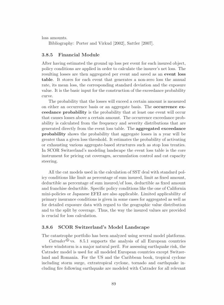
loss amounts.Bibliography: Porter and Virkud [2002], Sattler [2007].
3.8.5 Financial Module
After having estimated the ground up loss per event for each insured object,policy conditions are applied in order to calculate the insurer’s net loss. Theresulting losses are then aggregated per event and saved as an event losstable. It stores for each event that generates a non-zero loss the annualrate, its mean loss, the corresponding standard deviation and the exposurevalue. It is the basic input for the construction of the exceedance probabilitycurve.
The probability that the losses will exceed a certain amount is measuredon either an occurrence basis or an aggregate basis. The occurrence ex-ceedance probability is the probability that at least one event will occurthat causes losses above a certain amount. The occurrence exceedance prob-ability is calculated from the frequency and severity distributions that aregenerated directly from the event loss table. The aggregated exceedanceprobability shows the probability that aggregate losses in a year will begreater than a given loss threshold. It estimates the probability of activatingor exhausting various aggregate-based structures such as stop loss treaties.In SCOR Switzerland’s modeling landscape the event loss table is the coreinstrument for pricing cat coverages, accumulation control and cat capacitysteering.
All the cat models used in the calculation of SST deal with standard pol-icy conditions like limit as percentage of sum insured, limit as fixed amount,deductible as percentage of sum insured/of loss, deductible as fixed amountand franchise deductible. Specific policy conditions like the one of Californiamini-policies or Japanese EFEI are also applicable. Limited applicability ofprimary insurance conditions is given in some cases for aggregated as well asfor detailed exposure data with regard to the geographic value distributionand to the split by coverage. Thus, the way the insured values are providedis crucial for loss calculation.
3.8.6 SCOR Switzerland’s Model Landscape
The catastrophe portfolio has been analyzed using several model platforms.Catrader� vs. 8.5.1 supports the analysis of all European countries
where windstorm is a major natural peril. For assessing earthquake risk, theCatrader model is used for all modeled European countries except Switzer-land and Romania. For the US and the Caribbean book, tropical cycloneincluding storm surge, extratropical cyclone, tornado and earthquake in-cluding fire following earthquake are modeled with Catrader for all relevant
89

areas. Catrader performs analyzes of loss probabilities using aggregatedexposure data similar to RiskLink aggregated loss module. Like most catmodels, AIR applies a parametric approach for earthquake and tropical cy-clone modeling. For European extratropical cyclone, AIR has taken the leadin modeling the events based on a numerical simulation.
RiskLink� vs. 6.0 is applied for modeling Japanese typhoon and earth-quake risk. Basically, RiskLink differentiates between two types of loss mod-eling: The detailed loss module (DLM) suits flexible modeling of individualrisks whereas the aggregated loss module considers a variety of policy mar-ket assumptions for standard coverages (incl. proportional and first losspolicies) as well as for market specific coverages like fire expense insurance(EFEI) or Zenkyoren for Japan. Where reasonable, earthquake risks havebeen modeled by location, whereas the sum insured for typhoon risks aregenerally analyzed aggregated on CRESTA-zone or Prefecture level.
Sharp is a probabilistic in-house modeling platform, which models thelosses of a stochastic event set affecting a specific portfolio of exposed val-ues. Sharp can handle either detailed or aggregated exposure. Detailed lossmodeling can be performed down to a single location if sufficient address in-formation is provided, otherwise loss modeling is performed based on totalsums insured entered on an aggregated level (e.g. CRESTA) for given geo-graphic zones. The result is an event-loss-table, from which the exceedingprobability curve is derived. The event-loss-table can be directly importedinto the in-house pricing (MARS) and accumulation (GCDP) tools. Theevent-loss-table has the same format as the one of RiskLink. Sharp is usedfor modeling earthquake risk in Switzerland, Romania and certain areas inCentral and Latin America and South East Asia. For modeling wind risks,it is used for certain regions in South East Asia.
Table 3.3 depicts all loss potentials which are modeled stochastically.
Technical Documentation
AIR Earthquake Model Caribbean Region, Technical Document EQCAR-0206, June 2002
AIR Earthquake Models for Australia and New Zealand, TechnicalDocument EQAZ-0405, May 2004
AIR Earthquake Model for the Mediterranean Region, Technical Doc-ument EQMED-0206, June 2002
AIR Earthquake Model for the United States, Technical DocumentEQUS-0508, August 2005
AIR Extratropical Cyclone Model, European Region, AIR TechnicalDocument ETCEU-0607, July 2006
90
Peril Regions Model
Europe – windstorm Catrader/AIRMediterranean region – earthquake Sharp/SCOR
Catrader/AIRUS – earthquake and windstorm Catrader/AIRCaribbean – earthquake and windstorm Catrader/AIRMexico, Chile – earthquake Sharp/SCORJapan – earthquake and windstorm RiskLink/RMSAustralia, New Zealand – earthquake and windstorm Catrader/AIRRest of Asia – earthquake and windstorm Sharp/SCOR
Modeling regional Nat Cat portfolios. The commercial tools are Catrader,Risklink. The internally developed tools is Sharp.
Table 3.3: The Nat Cat model landscape at SCOR Switzerland.
AIR Severe Thunderstorm Model for the United States, Including Tor-nado, Hail, and Straight-line Windstorm, Technical Document STUS-0607, July 2006
AIR Tropical Cyclone Model Caribbean Region, Technical DocumentTCCAR-0311, November 2003
AIR Tropical Cyclone Model for Australia, Technical Document TCAU-0209, September 2002
AIR Tropical Cyclone Model for the U.S. Gulf and East Coasts, Tech-nical Document TCUS-0405, Sept. 2007
AIR Winter Storm Model for the United States, Technical DocumentETCUS-0508, August 2005
RMS� Japan Earthquake Model Methodology, November 2005
RMS� Secondary Uncertainty Methodology, September 2007
3.9 Stochastic Model for Run-Off Business
In this section we describe the stochastic model for run-off business. Weconsider the following types of cash flows:
� paid losses
� paid/received premiums
91

� paid external expenses (brokerage, commissions, etc.).
For simplicity, we assume that only the loss payments are stochastic, anduse deterministic estimates for the premiums and the expenses.
Consequently, to model the stochastic loss payments, the objective is todetermine the distribution of the basket mismatches
M bi = E[Rb
0 | Fi+1] − E[Rb0 | Fi] for i ≥ 0,
conditional on the information F0 available at time t = 0, and to specifythe dependency structure of the basket mismatches. To ease notation, M b
i
here denotes the mismatch, in year i, for the run-off business only. See pp.46 for the definition of the discounted outstanding reserves Rb
i for basket bat time t = i. Concerning the dependency structure of the run-off basketmismatches, see Section 3.9.4 (pp. 99).
Similarly as for the new business, we construct a model for the nominalbasket mismatches
E[Sb0 | Fi+1] − E[Sb
0 | Fi] (3.17)
where b denotes the basket and Sbi for i ≥ 0 denotes the nominal sum of the
future payments Xbj ,
Sbi :=
∑j≥i
Xbj .
In a second step, the nominal figures are transformed into cash flows anddiscounted using development patterns, see Section 3.2.2 (pp. 50).
With regards to the nominal basket mismatches from (3.17), these canbe expressed using the notation introduced in Section 3.2.3, pp. 52. To easenotation, we drop the superscript b denoting the basket in the following.
Since, using this notation,
E[S0 | Fi+1] − E[S0 | Fi] =(Xi + Si+1
)− Si,
the nominal basket mismatches provide a model for the one-year claimsdevelopment Qi,
Qi = Xi + Si+1,
where the reserves are best estimates in the sense that
E[Qi | Fi] = Si.
To split the one-year claims development Qi into payment Xi and reservesSi+1, we use the proposal from Section 3.2.3. That is,
Xi = ηi · Qi
Si+1 = (1 − ηi) · Qi
92

with ηi defined in (3.8).The following sections describe the derivation of the nominal basket one-
year mismatches from (3.17). In Section 3.9.1, we recall the definition ofdevelopment triangles and the well-known Mack model for the chain laddermethod. In Section 3.9.2, we outline our proposal for the calculation ofthe one-year change (3.17) for the first year i = 0. In Section 3.9.3, theprojection of the first year mismatches to future years is described. Finally,Section 3.9.4 discusses the proposed dependency structure.
3.9.1 Development Triangles, Chain Ladder, Mack Method
In this section we describe the different types of loss amounts consideredin the context of reserving, and we recall development triangles and theclassical Mack model for the chain ladder method (Mack [1993]). In thefollowing, all values are nominal. Typically, the calculations will be appliedto suitably defined sub-portfolios of the portfolio of run-off business.
For convenience, we denote, in this section only, the start year not byi = 0, as in the rest of the document, but by i = I + 1, in order not tohave to denote run-off underwriting years by negative numbers. The run-offportfolio thus consists of the run-off underwriting years i = 0, 1 . . . I.
The actuarial estimation of the reserves, at least for more mature years,is based on loss development triangles. With regards to these triangles, wecan distinguish different components of the estimated ultimate losses at agiven point in time:
estimated ultimate losses = paid losses + case reserves + IBNR,
reported losses = paid losses + case reserves,estimated reserves = case reserves + IBNR,
where
� paid losses are the nominal sum of all loss payments already booked,
� case reserves are estimates provided to us of the outstanding lossamounts for known losses (to be paid in the future),
� IBNR, short for incurred but not reported losses, denote our estimateof the difference between the reported and the actual ultimate losses.
Consequently, there are loss development triangles for paid, reported, andestimated ultimate losses.
As usual, calendar year i denotes the period from time t = i to timet = i + 1, and the first run-off underwriting year is i = 0. At the end ofcalendar year i = I, we consider
93

� underwriting years k = 0, 1 . . . , I,
� development periods j = 0, 1 . . . , I.
The development period j of one year is considered relative to the under-writing year k; consequently, i = k + j denotes the corresponding calendaryear.
Denote by Ck,j the cumulative reported losses for the underwriting yeark up to the end of calendar year k + j, i.e. at time t = k + j + 1. Let Tj bethe sum of the cumulative losses over all underwriting years in developmentperiod j, i.e.
Tj :=I∑
k=0
Ck,j . (3.18)
We assume:
� The ultimate loss is fully reported after I development periods.
The ultimate loss for accident year k is thus equal to Ck,I . The loss devel-opment triangle DI at time I + 1 consists of all entries Ck,j known up to theend of calendar year i = I, i.e. it is given by
DI := {Ck,j | k + j ≤ I} .
DI corresponds to the information on the losses available at t = I + 1. Anestimator of the cumulative paid loss Ck,j is denoted by
Ck,j ,
where the estimator is based on the information available at time t = I + 1.For convenience, we introduce the following notation to describe entries
in the most recent diagonal. Define the underwriting year j∗ = jI∗ and thedevelopment period k∗ = kI∗ relative to year I by
j∗ := I − j
k∗ := I − k.
At time t = I + 1, j∗ is the most recent underwriting year for which infor-mation is available about development period j and, similarly, k∗ is the thelargest development period for which information is available about under-writing year k.
At the end of year i = I, the sum Tj from (3.18) is estimated by
Tj :=j∗∑
k=0
Ck,j +I∑
k=j∗+1
Ck,j . (3.19)
94

The basket mismatches (3.17)
E[Sb0 | Fi+1] − E[Sb
0 | Fi]
then correspond to the difference
T′I − TI (3.20)
where the prime “′” denotes estimates at time t = I + 2, i.e. at the end ofthe following year I + 1.
To estimate this one year-change, in view of (3.19), we have to makeassumptions about
1. the method used to estimate Ck,j
2. a stochastic model for the random variables Ck,j ,
The second point is considered in Section 3.9.2. Concerning the first point,one such model is the classical Mack model for the chain ladder method.The Mack model for the chain ladder method is based on the following threemodel assumptions:
1. Different underwriting years k are independent. More precisely, therandom vectors (Ck,0, Ck,1, Ck,2 . . .) for different k are independent.
2. There exist positive development factors fj , called age-to-age factorsor chain ladder factors, such that
E [Ck,j+1 | Ck,0, Ck,1, . . . , Ck,j ] = fj Ck,j . (3.21)
3. There exist positive parameters σj such that
V ar[Ck,j+1 | Ck,0, Ck,1, . . . , Ck,j ] = σ2j Ck,j .
A few remarks about the Mack model:
� The Mack model is distribution-free: No assumption is made concern-ing the distribution type of the random variables Ck,j . The only as-sumptions made concern the first two moments of Ck,j . Consequently,it is likely that only statements about the first two moments of theestimation errors can be made.
� The first assumption in the Mack model, independency of different un-derwriting years, is questionable from a practical point of view, since,in reality, reserve increases are sometimes applied in one calendar yearto all underwriting years. This makes sense intuitively because certaincauses of dependencies (such as legal changes) apply to many under-writing years at the same time.
95

� Volatility in the Mack model comes from two sources: On the onehand, it comes from the deviation of the actual amount Ck,j+1 fromthe expected value fj Ck,j given the prior history (see (3.21)), whichis called stochastic error or process variance. On the other hand,volatility comes from the fact that the chain ladder factors fj exist butare unknown and have to be estimated from DI ; this is the estimationerror or parameter error.
� The assumption that the chain ladder factors exist but are unknownmight seem odd (e.g. in view of (3.21)). An alternative approach isto use a Bayesian view-point, see Gisler [2006]. In such an approach,the chain ladder factors are themselves random variables Fj , and theavailable information DI can be used to assess the distribution of theFj . When using a Bayesian approach, additional assumptions haveto be made regarding the prior distribution of the Fj and, in Gisler’spaper (Gisler [2006]), also regarding the distribution of the Ck,j .
� Consider the second Mack assumption (3.21). Per se, for a given un-derwriting year k, the expected value of the next amount Ck,j+1 giventhe prior history, i.e.
E [Ck,j+1 | Ck,0, Ck,1, . . . , Ck,j ]
is a function of the prior history Ck,0, . . . , Ck,j , where the functionmight depend on k and j. To arrive at (3.21), we need to make threeassumptions: The function depends on Ck,j only; the function is linearin Ck,j ; and the function depends on j but not on k.
Given the Mack model, at time t = I + 1, the ultimate loss Ck,I for under-writing year k can be estimated by
E[Ck,I | DI ] = E[Ck,I | Ck,0, Ck,1 . . .] = Ck,k∗
I−1∏l=k∗
fl. (3.22)
The first equality above is a consequence of the first Mack model assumption,and the second follows from repeated application of the second assumptionusing the appropriate version of the equality
E[X | Z] = E[ E[X | Y, Z] | Z].
Concerning again the first equality in (3.22), observe that this requires inde-pendency of the random vectors (Ck,0, Ck,1, . . .) and not just independencyof the random variables Ck,j for different k.
Moving to estimators of the involved quantities, the estimators fj for fj
given by
fj :=∑j∗−1
k=0 Ck,j+1∑j∗−1k=0 Ck,j
96

are unbiased and uncorrelated, and an unbiased estimator of (3.22) is givenby
Ck,I = Ck,k∗
I−1∏l=k∗
fl.
Mack then derives an estimate of the mean squared error mse(Ck,I)between the true ultimate Ck,I and the estimator Ck,I , given DI ,
mse(Ck,I) := V ar(Ck,I − Ck,I | DI) = E
[(Ck,I − Ck,I
)2 | DI
].
This error estimates the volatility of the “ultimate change,” i.e. the differ-ence between the current estimate Ck,I and the true ultimate Ck,I . For theSST, however, we need an estimate for the one-year change from (3.20),
T′I − TI ,
i.e. the difference between the estimate at t = I + 2 and the estimate att = I + 1. This problem is considered in the following section.
3.9.2 The One-Year Change for the Run-Off Business
In this section, we consider the question of how to estimate the one-yearchange from (3.20),
T′I − TI . (3.23)
In terms of the development triangle, the task is to estimate how the ultimateloss estimate TI changes when an additional diagonal in the developmenttriangle becomes known.
In the notation introduced in Section 3.9, the nominal one-year changeis written (shifting back from time t = I + 1 to time t = 0 for convenience)
Qi − Si,
with the one-year claims development
Qi = Xi + Si+1.
In a first step, we consider the estimate of the mean square error, i.e.the standard deviation of the one-year change (3.23).
We then make the following distribution assumption:
� X0 and S1 are log-normal distributed.
This assumption is standard for random variables for which extreme eventshave been removed.
Concerning the estimate of the mean square error, a method has beenproposed by Merz and Wuethrich in Merz and Wuthrich [2007] to estimate
97

the mean-squared error for the one-year change (3.23). This method is basedon a so-called time series model for the chain ladder method, which makesstronger assumptions than the Mack model and applies thus to a subsetof the Mack model. As for the “ultimate change,” the variance naturallydecomposes into a process variance (“stochastic uncertainty”) and an es-timation error (“parameter uncertainty”), and estimators are provided forboth quantities. The method was proposed to FOPI and has been approved.
Recently, an alternative approach has been developed by Markus Duerrin a currently unpublished paper. This approach does not assume the abovetime-series model but only the three Mack model assumptions.
We have compared the mean-squared estimates from the two methodson triangles from our reserving figures. As a general rule, the two figuresare quite close, with the Duerr method giving a slightly larger estimate.However, for a reserving analysis it is crucial to be able to handle incompletetriangles and data errors. Unlike for the Merz-Wuethrich method, for theDuerr method there exists a mathematically precise derivation of the mean-square error also in case certain link ratios in the triangle are excluded- which more closely mirrors the way reserves are actually estimated byreserving actuaries. For these reasons we propose to use the Duerr method.
Further note that the derivations of the estimators for the Duerr methodappear to be more straightforward and simpler than those in Merz andWuthrich [2007]. Moreover, Duerr explicitly compares the estimators fromthe two approaches and provides arguments for why his method seems prefer-able.
3.9.3 Projection to Future One-Year Changes
To calculate the expected shortfalls of the future one-year changes, we pro-pose to follow the approach outlined in Section 2.2.3 (pp. 35). That is, wespecify a proxy for the shortfall ratio (for basket b and calendar year i ≥ 2),
ξ(i)b =
ESα[M bi ]
ESα[M b1 ]
, (3.24)
where ES denotes the expected shortfall. We propose (see also pp. 50):
� The proposed proxy for the shortfall ratios ξ(i)b from (3.24) is the in-
cremental reported pattern by calendar year for basket b.
Recall that the reported pattern measures the estimate of the ultimateamount not considering IBNR. Incrementally, this corresponds to the one-year change M i
b of the reported loss amount. This pattern is usually longer-tailed than the pattern of the estimated ultimate loss including IBNR.
98

3.9.4 Dependency Structure and Aggregation for Run-OffBusiness
Since we do not have a detailed study of temporal dependencies available, wepropose to use the same dependency parameters in the portfolio dependencytree for the run-off business as for the new business, see Section 3.3.2 (pp.59).
This assumption might be questioned by arguing that the at least cer-tain extremal dependencies are manifested in the first year i = 0, so that thedependency between run-off business baskets ought to be reduced. However,for long-tail business, only very little information about the ultimate out-come is assumed to be revealed in year i = 0, so that “catastrophic events”(such as changes in law) occur during the run-off period. This implies, inparticular, that extremal dependencies for long-tail business are manifestedprimarily during run-off. This leaves the dependencies for short-tail busi-ness. However, for short-tail business, the shortfall contribution to run-offmismatches is expected to be small anyway, so that dependencies will nothave a big impact.
Concerning the definition of the run-off baskets, the granularity will pre-sumably not be selected as fine as for new business, in order to get reliabletriangles. Currently, the following run-off baskets are used
� Agribusiness
� Aviation
� Credit and Surety
� Engineering
� Marine
� Property
� Liability
� Professional Liability (excluding MDU, which is modeled separately)
� Workers Compensation
� Non-life Personal Accident (PA)
� Motor
� Miscellaneous
For the legal entity Cologne, only Property, Engineering, Marine, Liability,Motor, and Non-Life PA are considered, and the remainder is included inthe basket “Other.”
99
3.9.5 Data Requirements and Parameter forRun-Off Business
We summarize the requirements on the SST run-off business model.
� Definition of the run-off business baskets.
� Reserving development triangles of the reported/incurred losses byunderwriting year and development period to calculate the one-yearchange.
� Initial balance sheet reserves and premiums receivable and expensespayable
� Calendar-year earnings pattern
� Portfolio dependency tree to express the dependency structure betweenrun-off baskets, including dependency parameters, see Section 3.9.4(pp. 99).
� Method to estimate future (shortfalls of) one-year basket changesESα[M b
i ] for i = 1, 2 . . ., see pp. 98. According to this specification,we need, for each run-off basket,
– Incremental development pattern for incurred/reported losses bycalendar year.
� Development patterns for paid premiums and paid losses by calendaryear from reserving development triangles, see also Section 3.2.2 (pp.50).
3.10 Model for Non-Life Internal AdministrativeExpenses
A market-consistent valuation of liabilities requires modeling the costs ofdoing business. In particular, we have to consider administrative expenses,also called internal expenses, since these are an integral part of the produc-tion costs of a liability, and are to be viewed as part of the value of theinsurance liabilities. For this reason, we consider internal expenses bothin the context of solvency assessment for the SST and for the pricing ofcontracts at renewal.
The approach presented here was developed by Christoph Hummel anddescribed in the document Cost model for SST (Hummel [2007a]).
100
3.10.1 Acquisition and Maintenance Costs
In view of the one-year perspective inherent in the SST methodology, theinternal expenses have to be split up into two classes:
� Acquisition costs
� Maintenance costs
Acquisition costs for a contract are the costs associated with the acquisitionof the contract under consideration, and hence they are incurred only in theyear the contract is written.
Maintenance costs are the costs for the administration of contracts al-ready written. These costs persist throughout a potential run-off period ofthe contract and thus are incurred in all years starting from the year thecontract is written up to the year the contract is closed.
Obviously, this maintenance period depends on whether the contract isshort or long tail. Maintenance costs likely arise both from the payment ofclaims as well as from the reserving of claims. For a given year, it seemsreasonable to measure the maintenance costs for claims payment by the per-centage of the ultimate loss paid in this year, and the maintenance costs forclaims reserving by the outstanding reserves as a percentage of the ultimateloss.
The situation now is the following: Administrative expenses are providedby the finance department for a financial, i.e. calendar year, separate foreach legal entity. To simplify our exposition, we will in the following considerone specific legal entity but not specify the legal entity explicitly, and denoteby E0 the total administrative expenses for the non-life business of the legalentity under consideration. We must have available a breakdown of the totalexpenses E0 into acquisition costs A0 and maintenance costs M0,
E0 = A0 + M0.
These expenses arise from the liability portfolio in the books in year i = 0,which consist of business written in the underwriting years k = 0,−1,−2 . . . .The costs E0 consist of that part of the internal expenses for each of theseunderwriting years k which pertains to the year i = 0. Additional expenseswill arise for the underwriting year k business in the years i = 1, 2 . . . . Forthis reason we have to make an assumption about the future administrativeexpenses Ei for i = 1, 2 . . . .
For the future financial years i = 1, 2 . . . , we assume going concern withconstant volume, which implies that the administrative expenses Ei are con-stant except for inflation ai, so
Ei = Ai + Mi with Ai = ai A0, Mi = ai M0,
101

where we might take ai = (1 + θ)i for an average rate of inflation θ.Denote the administrative expenses from financial year i pertaining to
underwriting year k byEk
i = Aki + Mk
i .
Since acquisition costs only occur in the year a contract is written, we have
Aii = Ai, Ak
i = 0 for k �= i.
Concerning maintenance costs Mki , let
pki = percentage of ultimate loss for underwriting year k paid in year i
(incremental paid loss pattern)rki = percentage of ultimate loss for underwriting year k reserved in year i
(reserve (case + IBNR pattern)α = percentage of maintenance costs for claims reserving
(as opposed to claims payment)
We then assume that the maintenance costs Mki are given by
Mki = α Mi
rki∑
l≤i rli
+ (1 − α) Mipk
i∑l≤i p
li
for k ≤ i; Mki = 0 for k > i.
Assume for simplicity that administrative expenses pertain to mid yeari + 1/2. Let zi (t) be the value at time t ∈ {0, 1} of a zero coupon bondwith face value 1 in the currency of the legal entity under consideration,which matures at time i + 1/2. We do not model interest rate risk in theframework of internal expenses, so we approximate zi (1) deterministicallyusing the forward rates.
We can now calculate the internal expenses as a part of the value of theliabilities of the legal entity at time t ∈ {0, 1}. Indeed, the internal expensesIC (t) are composed of expenses pertaining to the underwriting years k ≤ t,
IC (t) =∑k≤t
ICk (t) ,
where the internal expenses ICk (t) for underwriting year k that have to bepart of the liabilities at time t consists of the discounted expenses whicharise in future financial years i = t, t + 1, t + 2 . . .. Hence, they are given by
ICk (t) =∑i≥t
zi (t) Eki .
102

3.10.2 Required Data and Discussion
Let us give an overview of the input data required for the administrativecost model:
1. Acquisition cost A0, LE and maintenance costs M0, LE for each modeledlegal entity in the financial year 0. For Cologne, we treat life and non-life separately.
2. For each legal entity, the aggregated paid loss pattern
3. For each legal entity, the reserve pattern (case + IBNR)
4. Expected average inflation (ϑ) for years 1, 2, · · ·5. Risk-free yield curve in the balance sheet currency at t = 0.
6. A numerical parameter α ∈ [0, 1] which defines the portion of mainte-nance costs to be modeled on the expected reserves.
We have pointed out how this approach is based on a going concern as-sumption at constant volume for the financial years i = 0, 1, 2, · · · , whichmakes sense from an economic perspective. Only in this way can we alignthe cost resulting from this valuation with the expenses allocated in pric-ing. It is also in line with the transfer approach taken in the SST. In thisframework, we need to consider in the valuation of the liabilities the cost forcapital and administration which a rational buyer would charge for takingover the corresponding liabilities. In our framework, the potential buyerwould be an identical copy of our company.
Finally, we mention an important difference between internal expenseallocation in SST and in pricing. In pricing, legal entities are not consid-ered separately, so the group’s overall internal costs for the underwritingyear k = 0 are allocated to the individual group’s reinsurance contracts inpricing, rather than allocating a legal entity’s cost to the legal entity’s rein-surance contracts. In this way we stick to our principle that the price for areinsurance contract is the same regardless of which legal entity it is written.
103

4
Life and Health Methodology
Our description of the internal risk models for the Life and Health businessis based on the document Methodology Life and Health, Gruetzner et al.[2007].
4.1 Structure of the Business
The L&H business is split in four lines of business (LoBs): Life, Health,Disability and Personal Accident. In addition to these lines we differentiatebetween the following types of business:
� GMDB business
� Financial reinsurance
� Short duration business
� Standard long-duration business
GMDB business
This is a portfolio of American variable annuities in run-off. Main exposureis to US-equity markets, i.e. asset risk, but being life insurance the portfoliois also to some extent exposed to more classical insurance risk.
Financial reinsurance
For our purposes financial reinsurance is described as long-duration insur-ance where financing aspects dominate. The classical insurance risk is lim-ited by various mitigating measures. For this reason the main exposure isto cedent default risk. Of course this type of credit risk is highly correlatedwith general asset risk.
104

Standard long-duration business
In addition to the special two types mentioned above, standard long-durationbusiness covers all the remaining long-duration business, i.e. mortality, dis-ability or other classical covers with long-term rate guarantees.
Short-duration business
Here the main exposure is to losses from short-term insurance risk. Thiscould be large-scale catastrophic events or high-concentration risk in oneexposed area. The run-off is also exposed to reserve risk as it is known fromnon-life business.
Guided by the above we have the following risk-categories to consider:
Asset risk
Here we refer to these asset risks which arise on the liability side of the busi-ness only. Clearly the GMDB business suffers if the underlying funds fallas the difference between funds value and guarantee in case of the insuredevent represents a loss to SCOR Switzerland Group. In case of the standardlong-duration business future losses are discounted less in situations withlower interest rates. This clearly leads to higher market values of losses intimes of low interest rates.
Credit risk – cedents
The finance re business has risk characteristics similar to a loan of SCORSwitzerland Group to the cedent, which is amortized over time. Clearly, ifthe cedent defaults, SCOR Switzerland Group incurs a loss equal to the lostamortization.
Fluctuation risk – L&H insurance risk
SCOR Switzerland Group insures the usual biometric risks mainly mor-tality (including accidental death) and morbidity. If due to pure randomfluctuation or a significant event affecting several insured risks negatively,e.g. a pandemic, the claims exceed the expected claims plus the safety mar-gin, SCOR Switzerland Group incurs a loss.
Trend risk – L&H insurance risk
For some risks the insurance coverage is long term, i.e. much longer thanone year and the premiums for this term is fixed in advance. In this case theinsurer faces the fluctuation risks mentioned above as well as the risk thatthe probability distribution for future points in time differs substantiallyfrom the probability distribution assumed when pricing the risk. This riskis called trend risk, an example would be deteriorating mortality rates dueto an increase to unhealthy behavior of insured persons.
105

4.2 GMDB
Definition and Exposure
The reinsured portfolio is retrocession of a portfolio of unit-linked contractswith Guaranteed Minimum Death Benefit guarantee (GMDB) sold in theUSA. Decreasing funds prices and / or increasing mortality and / or morerational policyholder behavior cause increased claims. Guarantee types arereturn of premium, ratchets, roll-ups and resets. Ratchet- and reset-featuresimply path-dependency of the guaranteed pay-off. For purposes of risk man-agement SCOR Switzerland Group has developed a stochastic cash flowmodel, which projects future cash flows using market-consistent asset sce-narios from a Hull-White model calibrated to current financial market data.This model reflects all treaty conditions and dynamic lapse depending onin-the-moneyness (ITM) of the guarantees. Additionally product featureslike dollar-for-dollar (�for� ) and partial withdrawal are reflected.
All actuarial assumptions have been checked and established in compre-hensive studies and additional consultations of the cedents. The model isexternally reviewed on a regular basis.
Risk factors influencing the GMDB exposure are
� Capital market risks
– The development of policyholder’s fund and hence the GMDB-pay-off is influenced by equities, bonds, interest rate and volatilitymovements.
– The GMDB-cover has characteristics of a derivative or option dueto its asymmetric pay-off.
� Mortality risk
– The portfolio is exposed to short-term fluctuation and trend risk:higher mortality implies higher notional of the embedded optionsand thus higher exposure.
� Policyholder behavior
– Policyholders have the right to (partially) withdraw their moneyat any point in time, thus stopping to pay guarantee charges andtherefore increasing the loss for SCOR Switzerland Group if theoption is out of the money.
– The pricing of the guarantee charges has been based on the as-sumption that a certain amount of policyholder lapses before theguarantee could come into effect, thus leading to reduced charges.If less policyholders lapse than planned in situations where theguarantee is in the money this also results in a loss for SCORSwitzerland Group.
106

– Policyholders can increase volatility by choosing different under-lying funds. If the level of volatility exceeds the planned levelthen this leads to a loss for SCOR Switzerland Group as theembedded options gain in value with increasing volatilities.
The GMDB portfolio is valued using a replicating portfolio approach.The replicating portfolio is a portfolio of assets closely matching the cashflows of the liabilities under all asset scenarios and consists of a set of fi-nancial instruments (candidate assets) which are easy to value, using closedform solutions. They are calibrated on a subset of the stochastic cash flowscenarios of the GMDB-liabilities. For a given set of financial scenarios themarket value of the GMDB liability can be easily determined at each pointin time using the replicating portfolio. This does not afford further MonteCarlo simulations and hence avoids the problem of stochastic-in-stochasticsimulations.
The replication portfolio itself varies with mortality and dynamic policy-holder behavior assumptions. For the calibration are best-estimate mortalityassumptions and best-estimate dynamic policyholder behavior assumptionsused. This allows reflecting all market risks precisely (e.g. developmentunderlying equity funds, change of interest rates and change of volatility).
Not reflected using the replication portfolio approach are the fluctuationand trend risk from mortality and trend risk for lapses. These risk typesare reflected by splitting market and mortality risk as follows. Mortalityrisk will be determined using a best-estimate asset-scenario. The resulting(mortality-)fluctuation risk is modeled and integrated into the fluctuationrisk model, as described there. Trend risk from mortality is modeled in thetrend risk model, as described there.
The risk of change in policyholder behavior is not modeled because of lowmateriality. An example: The impact of the worst case of �for� withdrawal(every policyholder maximizes the loss for SCOR Switzerland Group) resultsin an increase of the market value of the liabilities of only USD 25 million.As of 2007 we model 5% �for� withdrawal-rates and hence even a doublingof this rates only leads to an increase of only USD 1.25 million - and this isdiversifiable risk.
Stochastic Modeling
The GMDB replicating portfolio is considered in detail in Section 4.7 of thisdocumentation.
107
4.3 Finance Re
4.3.1 Definition and Exposure
First year financing strains of the cedents are financed by the reinsurerand the resulting debt is amortized over the lifetime of the treaty. SCORSwitzerland Group’s Finance Re portfolio is characterized by
� First year financing that exceeds the deferrable acquisition costs understatutory original terms
� An additional amortization margin contained in the reinsurance pre-mium
� At least partial claw-back of paid financing for lapsed policies
� Termination of the treaty after amortization, measured by an experi-ence account balance.
In order to qualify as reinsurance the treaties typically transfer somebiometric or lapse risk. But due to these risk mitigation features the pureinsurance risk is limited, e.g. a higher mortality or increased lapse ratesresult in a longer amortization period but the profitability remains nearlyunchanged and the setup of these contracts is close to debt instruments.
This immateriality of the insurance risk factors was verified by evaluatingthe impact of insurance risk scenarios at the 1% quantile. E.g. mortalitytrend, being normally distributed with standard deviation 5%, was set to112% · best estimate mortality. Lapse is the only risk factor where a contractexists that doesn’t amortize the financing, with an outstanding open balanceof less than 5% of the financing. We regard this effect as immaterial.
The only remaining risk is a thus default of the cedent, i.e. pure creditrisk.
4.3.2 Stochastic Modeling
The financial reinsurance portfolio of the SCOR Switzerland Group for lifeinsurance business consists of three contracts with three different counter-parties, defined in the economical sense, i.e. identifying all legal entitiesbelonging to the same group. In order to measure the impact of a default,the outstanding cash flows at each point in time of each contract have beenmodeled individually, fully reflecting the terms and conditions of the under-lying insurance and reinsurance treaties. All contracts with a single cedentare aggregated and modeled together, as a default is assumed to affect thewhole group. This deterministic cash flow projection is produced based onbest estimate assumptions and assuming no default. Hence the cash flowsin the best estimate scenario are all positive, representing the payback ofthe initial financing. In case of default all future cash flows are set to zero.
108

That means the present value of the lost amortization cash flows representsthe loss and we assume no recoveries.
The stochastic default scenarios are taken from the general credit riskmodel (see Part III of the documentation, pp. 303) so that they follow thesame methodology as in Non-Life.
Consistent with the SST-approach, for both life and non-life we look ata one-year time-horizon only. When valuing this one-year risk, the ratingcan either remain unchanged, drop to default or change to another rating.In case of a default the realized loss is the net present value of all future cashflows, as mentioned above. In any other case the cash flows are currently kepton their original value. This approach might be improved by consideringrating migration.
4.3.3 Dependency Structure
Because both market and credit information is included in the same scenarioset, it is thus ensured that the dependency between asset and credit risk isexplicitly modeled. As the cedents are insurance companies there will bea dependency between extreme insurance events and defaults of these com-panies, e.g. in case of a pandemic. Some extreme insurance events mayalso concern life and non-life business. Therefore this dependency betweenextreme insurance events and defaults is handled the same way for life andnon-life business when combining insurance and asset risks. The approachused has already been discussed for the non-life business in this documenta-tion (see the parts of this documentation on the Non-Life Liability Model).
4.4 Trend Risk
4.4.1 Definition and Exposure
Trend risk is defined as the risk that the assessment of initial best estimateassumptions changes over the one-year horizon. This could be due to incor-rect initial estimation (e.g. parameter risk in statistical estimates) or due tosystematic and unanticipated changes in the underlying risks (e.g. changesin incidence rates due to changing legal environment).
While this risk applies in principle to all insurance contracts, it has ma-terial consequences only in long-duration treaties. For this reason trend riskis only modeled for long-duration treaties within the L&H internal model.
SCOR Switzerland Group’s portfolio does not contain material treatiescovering longevity, long-term care or critical illness and the exposure oflong-duration treaties to health and personal accident is very limited.
Consequently the only material exposure to trend risk arises from riskfactors concerning mortality, lapse and morbidity. Since Finance Re treaties
109
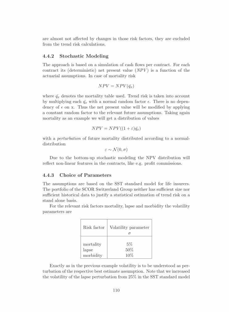
are almost not affected by changes in those risk factors, they are excludedfrom the trend risk calculations.
4.4.2 Stochastic Modeling
The approach is based on a simulation of cash flows per contract. For eachcontract its (deterministic) net present value (NPV ) is a function of theactuarial assumptions. In case of mortality risk
NPV = NPV (qx)
where qx denotes the mortality table used. Trend risk is taken into accountby multiplying each qx with a normal random factor ε. There is no depen-dency of ε on x. Thus the net present value will be modified by applyinga constant random factor to the relevant future assumptions. Taking againmortality as an example we will get a distribution of values
NPV = NPV ((1 + ε)qx)
with a perturbation of future mortality distributed according to a normal-distribution
ε ∼ N (0, σ)
Due to the bottom-up stochastic modeling the NPV distribution willreflect non-linear features in the contracts, like e.g. profit commissions.
4.4.3 Choice of Parameters
The assumptions are based on the SST standard model for life insurers.The portfolio of the SCOR Switzerland Group neither has sufficient size norsufficient historical data to justify a statistical estimation of trend risk on astand alone basis.
For the relevant risk factors mortality, lapse and morbidity the volatilityparameters are
Risk factor Volatility parameterσ
mortality 5%lapse 50%morbidity 10%
Exactly as in the previous example volatility is to be understood as per-turbation of the respective best estimate assumption. Note that we increasedthe volatility of the lapse perturbation from 25% in the SST standard model
110
to 50%. We felt that an increase was advised to cover additional lapse riskdue to potential asset movements, which are not directly modeled.
The volatility parameters above are also consistent with the stress sce-narios used by former SCOR Global Life to assess their capital requirementswithin the SCOR Group.
4.4.4 Dependency Structure
When varying the risk factors we apply the same perturbation to every treatyexposed to this risk. This means we assume no diversification within theportfolio. As the portfolio covers a great variety of cedents in a large numberof locations, we consider this to be a somewhat conservative assumption.
We assume the change of each of the risk factors to be independent.The result is then derived by adding up the cash flows, i.e. calculating theconvolution. The discounted best estimate will be derived by discountingwith appropriate yield curves. With the exception of GMDB and FinanceRe the specific treaties in our portfolio are known to exhibit no or onlynegligible dependency on market risk. So that discounting will be doneindependently from the values of the trend-risk factors.
Furthermore we assume independence between fluctuation risk and trendrisk.
4.4.5 Cash Flow Modeling
Almost all larger long-duration treaties are individually modeled. Thismeans the cash flows not only reflect the broader terms of the reinsuredportfolio but are also built on detailed assumptions about individual poli-cies which are either directly based on cedent data or derived from bookings.
Those same models are also used to derive US GAAP and IFRS figures.They are regularly updated and the models themselves as well as the under-lying best estimate assumptions are regularly reviewed by external parties.
Smaller treaties, where it is economically unfeasible to have individualmodels for each contract, are grouped into blocks of business with similarcharacteristics, as for example product types or geography. Cash flows forthese blocks are derived from historical observations of duration and resultratio.
4.5 Fluctuation Risk
4.5.1 Definition and Exposure
Fluctuation risk represents the uncertainty concerning losses deviating fromtheir expected value due to stochastic fluctuation within the one year timehorizon after valuation date.
111
Fluctuation risk should be seen in contrast to trend risk and reserverisk. For long-duration treaties fluctuations manifest themselves during theactual valuation year, while trends emerge in the actual year but impact allfuture contract years.
We assume also for short-duration treaties that fluctuation risk realizesitself and is completely paid during the one year time horizon. This is incontrast to reserve risk which exists only for run-off underwriting years.
The model refers to all treaties in-force during the valuation year. Forsimplicity reasons this portfolio was modeled by all short-duration treaties ofactual underwriting year and all long-duration underwriting years in-force.In-force short-duration treaties with premiums unearned in the actual bal-ance year arising from former underwriting years were not taken into ac-count. Consistent with that unearned premiums of the actual underwritingyear were included.
In principle all long- and short-duration treaties are exposed to fluc-tuation risk but because of the special contractual features of financing,fluctuation risk is not material and hence excluded from modeling.
Risk factors that determine the fluctuation risk are mortality, morbidityand accident incidences. Because of the one-year time horizon lapse is nosubstantial risk driver. Market risk drivers as interest rate changes or similarare not material.
The exposure of the GMDB portfolio to fluctuation risk is modeled atbest estimate assumptions regarding financial markets parameters and fur-thermore in consistence with the modeling of remaining US death cover.
4.5.2 Stochastic Modeling
As individual modeling on contract level is not available for the short-duration treaties, the portfolio exposed to fluctuation risk is separated intoclusters of treaties having similar risk profile. For a definition of risk clusterssee next section. The general approach is then to
� Model each risk cluster’s joint loss distribution
� Define and parameterize dependencies between risk cluster
� Aggregate the cluster distribution to a joint loss distribution of theLife fluctuation risk
The loss distribution of a single risk cluster is obtained by a collectivemodel. The collective model generally assumes that a realization of therandom variable total loss is given by a number of claims and the amountof loss of each claim.
Our interpretation of the collective model further assumes that the num-ber of claims is determined by the number of events and the number of claimsarising from a single event.
112

This approach provides an approach of parameterization of the distribu-tion of event separated from the distribution of the number of total claims.
Expressed in formulas the random amount of a cluster’s total loss S isthus defined as
S = X1 + X2 + · · · + XN
where Xi denotes the variable of single loss per event. Those severity vari-ables are assumed to be mutually independent and identically distributedaccording to a severity distribution. For further discussion of the Xi see thesection on parameter selection on p. 117. N denotes the random variable ofthe number of claims per event arising from the set of contracts.
We assume the frequency distribution N for the number of claims to be
N = M1 + M2 + · · · + MN
where N denotes the numbers of events happening during the year andMi the random variable of number of claims per event. Again all Mi are as-sumed to be mutually independent and identically distributed. The numberof events N is modeled as a Poisson distribution having mean value λ. Thedistribution of the number of claims per event M is either a zero-truncatednegative binomial tnb or a mixture of the tnb distribution and a Poissondistribution that gives additional weight to a predefined worst case scenariomtnb.
The unmixed frequency distribution tnb assigns very little probabilityto high numbers of claims per event. As an example (only illustrative sincee.g. a pandemic produces higher mean of total claims) the following exhibitshows probabilities below 0,01% of the negative binomial distribution withmean 1,8:
113
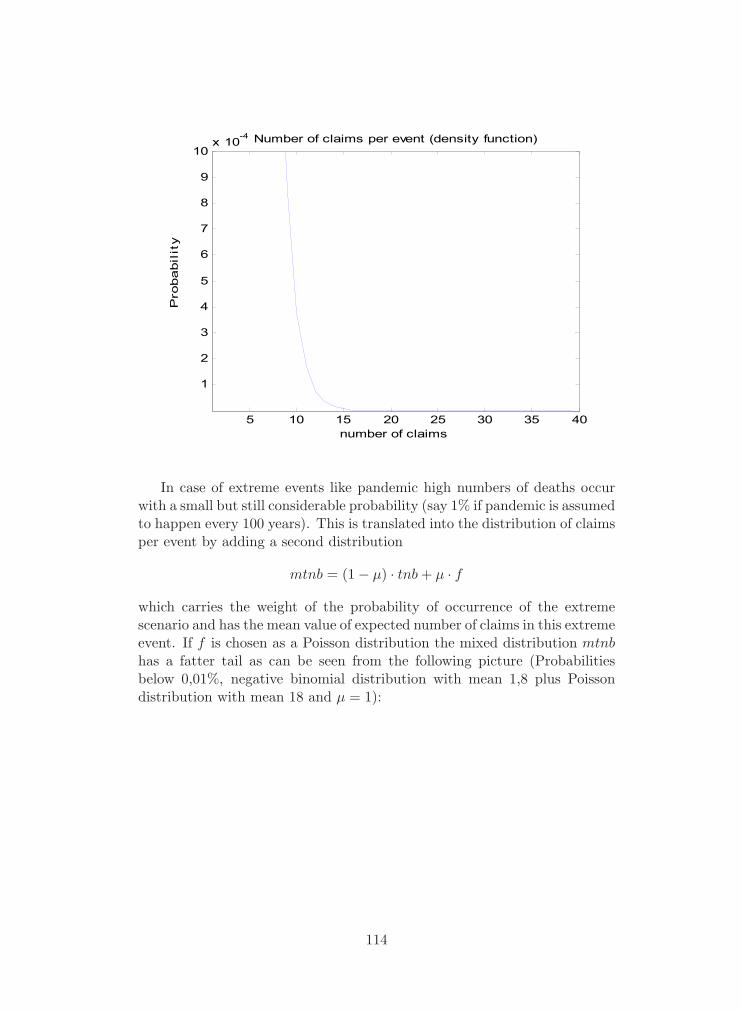
5 10 15 20 25 30 35 40
1
2
3
4
5
6
7
8
9
10x 10
-4 Number of claims per event (density function)
number of claims
Pro
babil
ity
In case of extreme events like pandemic high numbers of deaths occurwith a small but still considerable probability (say 1% if pandemic is assumedto happen every 100 years). This is translated into the distribution of claimsper event by adding a second distribution
mtnb = (1 − μ) · tnb + μ · f
which carries the weight of the probability of occurrence of the extremescenario and has the mean value of expected number of claims in this extremeevent. If f is chosen as a Poisson distribution the mixed distribution mtnbhas a fatter tail as can be seen from the following picture (Probabilitiesbelow 0,01%, negative binomial distribution with mean 1,8 plus Poissondistribution with mean 18 and μ = 1):
114
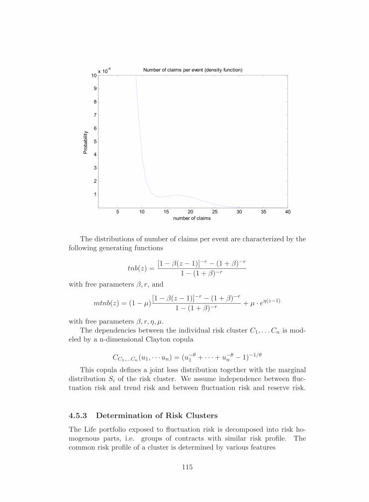
5 10 15 20 25 30 35 40
1
2
3
4
5
6
7
8
9
10x 10-4 Number of claims per event (density function)
number of claims
Pro
babi
lity
The distributions of number of claims per event are characterized by thefollowing generating functions
tnb(z) =[1 − β(z − 1)]−r − (1 + β)−r
1 − (1 + β)−r
with free parameters β, r, and
mtnb(z) = (1 − μ)[1 − β(z − 1)]−r − (1 + β)−r
1 − (1 + β)−r+ μ · eη(z−1)
with free parameters β, r, η, μ.The dependencies between the individual risk cluster C1, . . . Cn is mod-
eled by a n-dimensional Clayton copula
CC1,...Cn(u1, · · ·un) = (u−θ1 + · · · + u−θ
n − 1)−1/θ
This copula defines a joint loss distribution together with the marginaldistribution Si of the risk cluster. We assume independence between fluc-tuation risk and trend risk and between fluctuation risk and reserve risk.
4.5.3 Determination of Risk Clusters
The Life portfolio exposed to fluctuation risk is decomposed into risk ho-mogenous parts, i.e. groups of contracts with similar risk profile. Thecommon risk profile of a cluster is determined by various features
115

� Geography
� Product types
� Further contractual features (Limits, . . . )
� Underwriting and risk mitigation (Guidelines, accumulation control)
For the classification of contracts into risk clusters SCOR Switzerland Groupconducted an analysis of its business to asses the individual exposure withrespect to the above categories.
This analysis revealed that geography is an important indicator becauseextreme scenarios are often defined regionally. Also for global scenarios theimpact is modeled and evaluated by country (see description of pandemicscenario below).
Risk factors (mortality, morbidity, . . . ) translate into SCOR SwitzerlandGroup’s lines of business Life, Health, Disability and Accident. Althoughrisk factors are not explicitly modeled, the distinction of clusters by line ofbusiness is useful because related extreme scenarios are different. The expo-sure to lapse and financial market risk is within the one-year time horizonis negligible.
The risk assessment analysis further revealed that distinct contractualfeatures do not lead to substantially different risk profiles (at least when seefrom an aggregated perspective). The portion of non-proportional treatiesis low.
There are parts of the portfolio where exclusions reduce substantiallythe risk exposure. Health treaties in Middle East mostly exclude epidemicevents which reduces the exposure to pandemic1.
The distinction of individual sold policies and group covers is important(hence used for the risk clusters) because of degree of local risk concentra-tion.
Individual information on Underwriting guidelines, limitation of con-tracts or accumulation control was studied and did not define distinctionsin risk classes. This information was partly used for the estimation of sever-ity distribution, partly for assessing the impact of extreme events.
1These pandemic exclusions in the Middle East are watertight. There is an explicitand unequivocal clause in those treaties.
116

Region Duration LoB Premium Volume
Middle East Short Health 13%
Middle East Short Non-Health 3%
Central Europe Long Life 21%
Central Europe Short Life 16%
Italy Short Accident 6%
Sweden Short Disability 5%
Netherlands Long Disability 10%
USA, IRP treaties Long Life 7%
USA, GMDB Long Life 1%
USA, other Long Life 9%
Latin America Long Life 4%
Far East Long Life 5%
4.5.4 Choice of Parameters
The model of each risk cluster is calibrated to the expected loss of its port-folio. This expected loss is derived from
� Information provided by individually treaty models for the long-durationsegments Central Europe, Netherlands and IRP treaties
� Pricing data for the Swedish disability contracts
� The known number of policies and estimated incidence rates in caseof several short-duration segments
� An estimation of risk premium based on the US GAAP premium
The US GAAP premium used for calibration is the premium estimatedfor the actual balance year for long duration and for the actual underwritingyear for short-duration business. For simplicity reasons premiums unearnedin the actual balance year arising from former underwriting years were nottaken into account, unearned premiums of the actual underwriting year wereincluded.
Further input data are the number of risks and the average incidencerate of each cluster. The number of risks was deducted from the knownportfolio or reported on cedents accounts or estimated from information likepremium, expected loss or limitations per risk.
The choice of parameters of the various distributions comprises the fol-lowing steps:
117

� Determination of the frequency of events (parameter λ of the Poissonvariable N
� Determination of the frequency of claims per event (parameter β andr of the number of claims distribution)
� Determination of the severity distributions Mi
� Calibration of the single free parameter θ of the Clayton copula
The free parameters of the frequency distribution are determined by thefollowing conditions:
� The joint loss distribution has to reproduce the mean expectation ofloss supplied by pricing data (risk premium).
� The frequency of claim distribution (for some cluster the joint lossdistribution) should reproduce the impact of predefined extreme sce-narios.
� The modeled number of claims per event should correspond to a quan-tity observed in the portfolio or judged reasonable.
From the equation for expected values
E(N) = E(M)E(N)
it follows that the free parameter λ of the Poisson distribution of the numberof events is given by the expected number of total claims (which is estimatedby portfolio data as average incidence rate times number of policies) andthe mean value of the distribution of the number of claims per event. Asdescribed above the latter function is either a regular or an extended negativebinomial distribution.
The regular case that is applied to the non-pandemic dominated clusteris characterized by the parameters β and r. The parameters were chosen asfollows:
r is set to 1 for all clusters.
(1 + β) equals the mean value of number of claims per event. β waschosen individually for each cluster by Underwriting information (lowfor individual insurance, high for group insurance).
For the clusters dominated by the pandemic extreme scenario the fre-quency per event was modeled by the extended distribution mtnb. The freeparameters β, r, η, μ, were determined as follows:
� r as above.
118

� (1+β) equals the mean values of number of claims per event, as above.
� μ corresponding to the probability of occurrence of the extreme sce-nario.
� η corresponding to the excess mortality of pandemic scenario.
The determination and evaluation of extreme scenarios for each clusterrepresents the main tool of model calibration. For each cluster we defined aprincipal scenario and additional scenarios. The principal scenarios are thefollowing:
Region Duration LoB Scenario
Middle East Short Health Industry accident
Middle East Short Non-Health Pandemic
Central Europe Long Life Pandemic
Central Europe Short Life Pandemic
Italy Short Accident Earthquake
Sweden Short Disability No scenario
Netherlands Long Disability Pandemic
USA, IRP treaties Long Life Pandemic
USA, GMDB Long Life Pandemic
USA, other Long Life Pandemic
Latin America Long Life Pandemic
Far East Long Life Pandemic
The impact of pandemic on the portfolio was modeled in accordance withthe approach used for the FSAP scenarios. The excess mortality applied toregional business is the following.
800%Far East
300%Middle East
60%Americas
100%Europe
Excess mortalityRegion
As secondary extreme events we considered basically two scenarios withinareas of high population density:
� Terror attack (minor: explosion destroying huge building, similar toWTC or major: Anthrax attack, spread of deathly poison among ur-ban area)
119

� Industry accident (contamination of urban popularity with poisonousgas released by train crash)
The calibration of the Clayton copula parameter was based on the impactof all mentioned scenarios.
4.5.5 Technical Modeling
The generation of the loss distributions of the risk clusters as well as theaggregated loss distribution is based on MatLab code.
Once the free parameters of the frequency distribution are set by thecalibration process and the severity distribution is determined the MatLabprogram calculates the joint loss distribution of each cluster using a FastFourier algorithm.
The modelling of the risk cluster is based on actual portfolio data. Infor-mation on cluster volumes are based on the US GAAP estimated premium.
4.6 Dependency Structure of the Risk-Categories
In order to manage the approach, we make the following assumptions on thedependency structure:
� There is no dependency between the trend risks and all other risk-categories.
� There are dependencies between asset and credit risks – these arereflected in the central asset and credit risk model.
� There is a (tail) dependency between all insurance risks (includingnon-life) and asset risks . The underlying assumption is that majorinsurance events can influence the financial markets. This effect isreflected on the level of the overall integration.
� There will be a tail dependency between L&H insurance risks andcredit risks. The underlying assumption is that major L&H insuranceevents could lead to the insolvency of L&H insurers and thus to lossesin SCOR Switzerland Group L&H finance Re portfolio. This effect isagain reflected on the level of the overall integration.
We can determine the loss distribution for the different areas separately,because
� The fluctuation risks and trend risks are regarded as independent
� All potential asset risk dependencies are reflected by using the centralasset scenarios where necessary, i.e. for the GMDB (market risks) andFinance Re portfolio
120

� The GMDB portfolio is split into a market risk, a fluctuation risk anda trend risk part (see the section on GMDBs, pp. 121)
Table 4.1 summarizes all partial models and their aggregation.
Asset and credit risk scenarios, central model
Total
...
Fluctuation risk
(including GMDB-insurance risks)
Cluster 1 Cluster nGMDB
(market-risk)...Finance
Re
claim-scenarios, asset-dependentclaim-scenarios
Copula-approach
claim-scenarios, cash-flows
Combining assets and claims, reflecting dependency structure betweeninsurance risk factors and asset and credit risk
and discounting of trend risk components
Cluster n
Total
...
Trend riskRisk factor 1 Risk factor n...
Non-life
Overall distribution and Expected Shortfall
In scope
independent
independent
Combining life and non-life, reflecting dependency structure
(for trend risks based on asset-independent approximation)
Table 4.1: Life business: Partial models and their aggregation.
4.7 The GMDB Replicating Portfolio
The liability cash flows generated by GMDB (Guaranteed minimum deathbenefit) contracts (Life Insurance) are narrowly matched by a portfolio con-sisting of European put options, European look-back put options, bonds andequities (Erixon and Kalberer [2005]).
The GMDB cash flows could equally be replicated by futures and swaps,which are traded in a deep and liquid market. This would lead to a minorlack of precision with respect to calibration of the model to market values.The precise choice of financial instruments (European look-back put options)in the replicating portfolio is for purely technical reasons: Instruments withgood replication properties and closed valuation formulas were chosen.
The scenarios used for the GMDB model are fully consistent with thebootstrapping-the-economy model (Chapter 10). Market consistent scenar-ios are used for determining the market value. While calibration of thereplicating portfolio is (up to statistical error) independent of the economic
121

scenarios used, the same economic scenarios are used for valuation of thereplicating portfolio as for any other assets.
The composition of such theoretical portfolios is determined by theSCOR Switzerland’s Actuarial Life and Health team in Cologne based onstochastical projections of the future cash flows and numerical methods(Moore-Penrose inverse). The replicating portfolio allows an evaluation ofGMDB in stochastic scenarios via usual option pricing formulas.
A GMDB is a Guaranteed Minimum Death Benefit based on the con-cept of variable annuities. Payments are variable with respect to their leveland the exact time at which payments occur. The premium paid by thepolicyholder is being invested in equity funds, bond funds, mixed funds.Contingent on the specific policy the insured person may choose amonga variety of funds and may even switch funds during the runtime of thetreaty. The GMDB product in this sense is not so much an income supportfor retirement; primarily it offers the opportunity of tax-deferred financialinvestments. Any policyholder will hold an account of assets in equities,bonds and the money market.
The risk which SCOR Switzerland accepts is the guaranteed value incase of death, the GMDB, during the deferment period. SCOR Switzerlandcovers the difference between the account value and the GMDB in the mo-ment of death of the insured person. The capital at risk is the differencebetween the account value and the GMDB. In case of death of the insuredindividual during the surrender charge period, SCOR Switzerland mighthave to pay surrender charge additionally. SCOR Switzerland receives asa reinsurance premium a percentage of the current account value. Typesof guarantees include ROP, ratchet and roll-up. With the ROP, Return ofpremium, at minimum the premium will be paid out in case of death. Theone-year ratchet annually adjusts the death benefit to the account value incase this is higher than the death benefit up to then, so cash flows depend onthe maximum asset value reached at previous policy anniversaries. Roll-upmeans that the GMDB annually grows by a percentage independent of theaccount value until a ceiling is reached. Proportional withdrawals do not af-fect the ratio of GMDB to account value while dollar-for-dollar withdrawalswill. Dollar-for-dollar withdrawals reduce the GMDB and the account valueby the same nominal amount.
GMDB treaties are long duration contracts. The projection length ofthe stochastic scenarios is 30 years. For the purpose of the stochastic modelthe mortality, the partial withdrawals and any lapses are deterministic. Theonly stochastic variable is the performance of the assets. The calculationof net present values (NPVs) is based on cash flows. Premiums receivedby SCOR Switzerland are a percentage of the account value. Given theprojected cash flows from the comprehensive stochastic model, a so-called
122

replicating portfolio consisting of a set of financial instruments is calibratedand then used to integrate GMDB into SST.
How to replicate GMDB liabilities by market portfolios is described inErik Erixon and Tigran Kalberer, REPLICATING PORTFOLIO (Erixonand Kalberer [2005]). The document introduces the replication method. Itdoes specify the classes of assets to be used under the replication. Numer-ical illustrations and practical examples which the document presents shallmerely serve as a demonstration of the method’s applicability. They alsoillustrate how the calibration is done. It is understood that the implemen-tation of the model under real conditions required hundreds of options withan almost continuous range of strike prices when the GMDB document (Er-ixon and Kalberer [2005]), in order to elucidate the basic mechanisms, wasbound to select among a narrowly confined amount of merely ten or twentyof these assets.
In the following we will describe the procedures and methods used toset up and calibrate a replicating portfolio that replicates the cash flowsof the GMDB business. The GMDB business by SCOR Switzerland con-sists of several cedents and more than one million reinsured and retrocededpolicies. These can through methods of condensing be modeled accuratelyusing approximately 150’000 model-points that are representative of thebusiness. In order to simulate the behavior of the market value and themean NPV2 significant speed requirements are posed on the model. Pro-jecting one stochastic-within-stochastic scenario for one time period, i.e.projecting the business forward one period and then calculating a new mar-ket value using Monte Carlo simulations, takes around 30 hours using thecurrent seriatim GMDB model. This is not a feasible approach. Below wewill show that a portfolio of assets can be found, which replicates the totalcash flows of the portfolio accurately enough and which can be valued usingclosed-form solutions. This replicating portfolio can then replace the realportfolio for all simulation purposes which will increase computation speedsignificantly but also will reduce the impact of potential calibration errors ofthe economic scenarios used for valuation purposes. The difficult part of thereplicating portfolio approach is to determine a set of assets which may becombined to constitute the replicating portfolio. Essentially assets need tobe found that have the same characteristics and dependencies as the GMDBportfolio itself. In this section we are going to describe methods of findingthis set of assets and calibrating a replicating portfolio to the real portfolio.In order to find the appropriate set of assets we need to have a closer lookat the contracts and the definition of the policyholder benefits.
2The mean NPV is defined as the average of the net present values of 1’000 real worldscenarios, discounted at a rate currently set to 5%.
123

4.7.1 Determining a Set of Replicating Assets
Return of Premium and Roll-up GMDBs
The most basic GMDB covers are the return of premium (ROP) and the roll-up GMDB covers. We can assume that the pay-off of such GMDB is strictlydependent on the asset index (AI) at the time of the pay-off, assuming thatthe policyholder behavior is a known deterministic factor, independent fromthe past behavior of the assets. The pay-off of a ROP contract in one timeperiod t is calculated as
Claimt = max (0, GMDBt − AVt)(
lx+t−1 − lx+1
lx
)
where
GMDBt =t∑
i=issue
Pi
is the sum of the premiums paid until time t and
AVt =∑
i=issue
P ti
(AIt
AIi
)
is the account value at time t. Since there are very few premiums paidinto the account value (AV) currently, we can assume that there will be nofuture premiums after valuation. Thus, the account value for each contract(or model-point) can be rewritten as
AVt
=valuation∑i=issue
Pi
(AIt
AIi
)
=(
AIt
AIvaluation
) valuation∑i=issue
Pi
(AIvaluation
AIi
)
= f (AIt)
where the function f symbolizes that the only stochastic variable is theasset index AIt at time t, all other variables are already fixed. Certainlylapses and partial withdrawals will also affect the account value, although forthis purpose it shall be assumed that these are deterministic assumptions.Premiums are also payable to SCOR Switzerland by the cedents, these arestrictly dependent on the account value at every point in time3
Premiumt = Rate · AVt
3For some products there are maximum premium limits, an amount in USD after whichthe premiums do not increase by the account value.
124
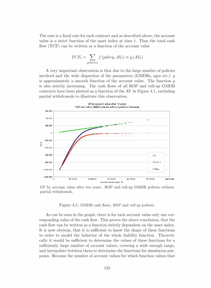
The rate is a fixed rate for each contract and as described above, the accountvalue is a strict function of the asset index at time t. Thus the total cashflow (TCF) can be written as a function of the account value
TCFt =∑
policies
f (policy, AVt) ≡ g (AVt)
A very important observation is that due to the large number of policiesinvolved and the wide dispersion of the parameters (GMDBs, ages etc.) gis approximately a smooth function of the account value. The function gis also strictly increasing. The cash flows of all ROP and roll-up GMDBcontracts have been plotted as a function of the AV in Figure 4.1, excludingpartial withdrawals to illustrate this observation.
CF by account value after ten years. ROP and roll-up GMDB policies withoutpartial withdrawals.
Figure 4.1: GMDB cash flows, ROP and roll-up policies.
As can be seen in the graph, there is for each account value only one cor-responding value of the cash flow. This proves the above conclusion, that thecash flow can be written as a function strictly dependent on the asset index.It is now obvious, that it is sufficient to know the shape of these functionsin order to model the behavior of the whole liability function. Theoreti-cally it would be sufficient to determine the values of these functions for asufficiently large number of account values, covering a wide enough range,and interpolate between them to determine the functions for simulation pur-poses. Because the number of account values for which function values that
125

need to be evaluated is small compared to the number of model-points in-volved, this would imply that the determination of the cash flows for eachscenario requires at most two calculations instead of 160’000 (approximatelythe number of model points). This is a significant improvement.
But we want to go a step further. We want to approximate the cash flowfunction by the sum of functions which represent the cash flows of derivativesthat have closed-form solutions to the market value. The portfolio consistingof these derivatives then replicates our liability portfolio and its value can bedetermined using closed-form solutions which is extremely helpful for a lotof relevant applications. In order to determine this replication portfolio it isin fact only necessary to evaluate the cash flow function over a sufficientlywide range of account values, it is not necessary to use account values,which have been produced by scenarios. Using appropriately calibratedscenarios just ensures that areas of account values which are more frequentlyhit by scenarios are evaluated with a higher granularity than other areasof less importance. Thus it is not important whether the scenarios usedfor fitting a replication portfolio are accurately reflecting current marketconditions. It is of higher importance that the area of possible account valuesis sufficiently spanned by the scenarios in order to prevent extrapolationerrors. By inspection of the graph we decide to choose the following assetsto determine the replication portfolio:
� An asset with the pay-off of the underlying account value itself
� A fixed cash flow (zero bond) and
� European put options on the asset index with different strike prices
The asset paying the account value itself will then replicate the premiumsand the European put options will replicate the claims. The slope of the putoptions has to be smoothed into the cash flow curve. Such a slope can becreated by combining several European put options with different strikes. Itis very important to ensure that the replication portfolio is well behaved forvery small and very large account values. Otherwise scenarios which producevery small or large account values would not be valued appropriately whichcould cause substantial distortions. In our case the asymptotic behavior ofthe replication assets and the portfolio is the same, which ensures that thisproblem will not arise (as can be seen in the graph).
A complicating matter for the ROP and roll-up GMDBs is the dollar-for-dollar withdrawals, which do not affect the account value and the GMDBin a proportional manner as normal partial withdrawals do. While the ac-count value decreases by a percentage which is equal to the rate of partialwithdrawal, the GMDB amount will be decreased by a proportionally dif-ferent amount. This creates a dependency on the path of the asset indexuntil time t. In Figure 4.2 the cash flows which include the effect of partialwithdrawals have been plotted as a function of the account value.
126

CF by account value after ten years. ROP and roll-up GMDB policies.
Figure 4.2: GMDB ROP and roll-up, including partial withdrawals.
As can be seen, the premiums are still strict functions of the accountvalue while the claims are now also dependent on another variable, notvisible in this graph, and are therefore not a function strictly dependent onthe account value. Although the claims are somewhat scattered, the basicshape of the dependency can still be clearly observed. We have producedan example of how the GMDB cash flows can be replicated using Europeanput options4 in Table 4.2. The pay-offs of the options are plotted in Figure4.3.
As can be seen, the claims are not perfectly replicated, the dollar-for-dollar withdrawals being the main reason for the differences. It can also beobserved that the pay-offs of the replicating portfolio are piecewise linear,the reason being the limited number of options used to replicate the cashflows. Since there are closed-form solutions available for the European putoptions the market value and the mean NPV can easily be calculated whileprojecting the business forward. The premiums can be replicated using asimilar method.
4For the purpose of this example we have excluded the premiums. Replicating thepremiums by an appropriate volume of investments into the underlying account valueshould be a straightforward exercise.
127

Asset Strike Number of assetsEuropean put option 1 0.8 0European put option 2 1 208583European put option 3 1.111 -216250European put option 4 1.667 -167369European put option 5 2.222 -228732European put option 6 2.778 -40322European put option 7 3.333 -45794European put option 8 3.889 -41517European put option 9 4.444 -37240European put option 10 10 5532
Table 4.2: GMDB: Replication of the roll-up and ROP pay-off
CF by account value after ten years. ROP and roll-up GMDBpolicies.
Figure 4.3: GMDB: pay-offs of options.
128

Ratchet Policies
Ratchet GMDBs are dependent on the maximum of the asset index as wellas the asset index at the time of the cash flow. This means that the claimswill be written as a function of the maximum of the asset indices, AImax,up to time t and the account value at time t.
Cash flowt = f (AIt, AImaxt)
So these liabilities are dependent on two factors instead of one. But the basicapproach will be the same as for the ROP GMDBs. When actually model-ing ratchet GMDBs there are two features which also need to be considered.The ratcheted GMDB amount is set to the maximum of the GMDB coverof the previous period and the asset index only once per year. To enablecondensing of policies with different quarter of ratchet, each policy is splitinto four different parts which are ratcheted once per year on the four cal-endar quarters respectively. This means that the claim amount for a singlepolicy will be dependent on the asset index at the time of the payout andthe maximum of the asset index of the four quarters (referred to as AImaxqX
for quarter X) separately
Cash flowt = f(AIt, AImaxq1t
, AImaxq2t, AImaxq3t
, AImaxq4t
)Several of the ratchet products have a maximum age after which the GMDBamount is no longer increased. After that age the GMDB amount equalsthe amount as at that date. For a policy where the ratchet cover expired ata prior time z the cash flow can be written as
Cash flowt = f(AIt, AImaxq1z
, AImaxq2z, AImaxq3z
, AImaxq4z
)Figure 4.4 shows a surface plot of the cash flows from one ratchet GMDBpolicy by the asset index and its maximum. The policy simulated onlyincludes one of the four quarter parts described above, the third quarter,and the maximum asset index, plotted on the x-axis of the graph, takesinto account the maximum ratchet age as described above. Dollar-for-dollarpartial withdrawals have also be set to zero in order to single out a policythat is strictly dependent on the asset index and its maximum.
As can be seen above, the plot shows a surface strictly dependent on themaximum of the third-quarter asset index, the asset index at valuation andthe maximum ratchet age. This proves that the conclusions made aboveare correct. In the remainder of this section we will add on the featuresdescribed above to show which of these are material and which are not. Fig-ure 4.5 displays the graph of a policy also run with dollar-for-dollar partialwithdrawals.
The surface is now somewhat distorted by the dependency on the pathof the asset index. If the quarterly parts 1, 2 and 4 are also included theresult is Figure 4.6.
129

Figure 4.4: Surface plot of GMDB cash flows (ratchet policy)
Figure 4.5: Surface plot of GMDB cash flows including dollar-for-dollar with-drawals.
130
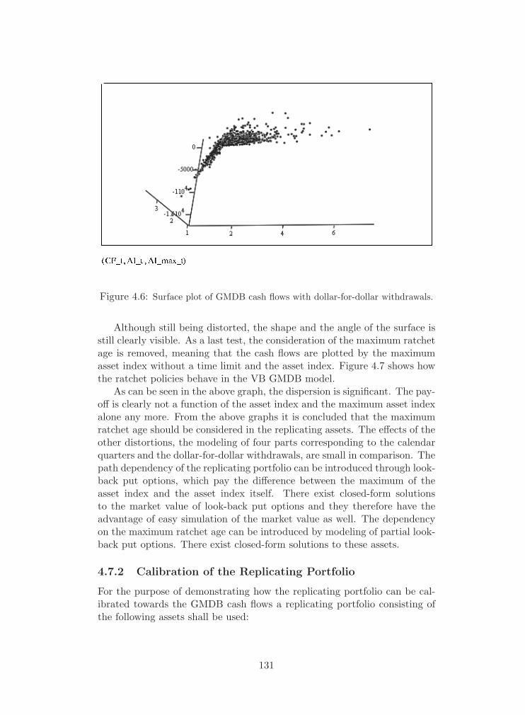
Figure 4.6: Surface plot of GMDB cash flows with dollar-for-dollar withdrawals.
Although still being distorted, the shape and the angle of the surface isstill clearly visible. As a last test, the consideration of the maximum ratchetage is removed, meaning that the cash flows are plotted by the maximumasset index without a time limit and the asset index. Figure 4.7 shows howthe ratchet policies behave in the VB GMDB model.
As can be seen in the above graph, the dispersion is significant. The pay-off is clearly not a function of the asset index and the maximum asset indexalone any more. From the above graphs it is concluded that the maximumratchet age should be considered in the replicating assets. The effects of theother distortions, the modeling of four parts corresponding to the calendarquarters and the dollar-for-dollar withdrawals, are small in comparison. Thepath dependency of the replicating portfolio can be introduced through look-back put options, which pay the difference between the maximum of theasset index and the asset index itself. There exist closed-form solutionsto the market value of look-back put options and they therefore have theadvantage of easy simulation of the market value as well. The dependencyon the maximum ratchet age can be introduced by modeling of partial look-back put options. There exist closed-form solutions to these assets.
4.7.2 Calibration of the Replicating Portfolio
For the purpose of demonstrating how the replicating portfolio can be cal-ibrated towards the GMDB cash flows a replicating portfolio consisting ofthe following assets shall be used:
131
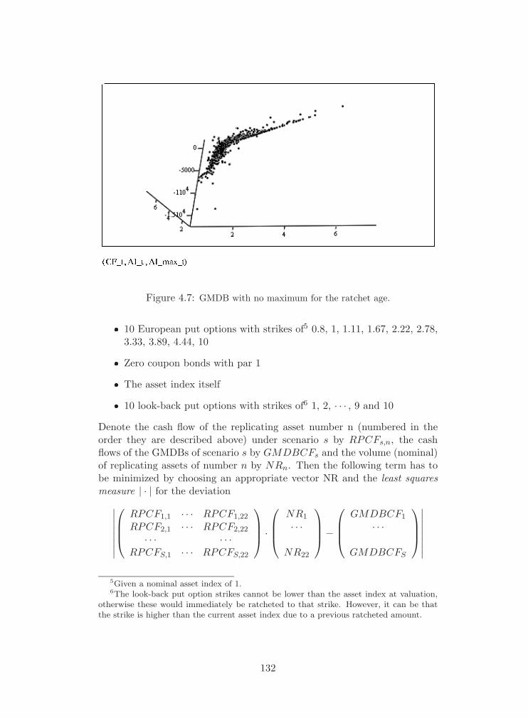
Figure 4.7: GMDB with no maximum for the ratchet age.
� 10 European put options with strikes of5 0.8, 1, 1.11, 1.67, 2.22, 2.78,3.33, 3.89, 4.44, 10
� Zero coupon bonds with par 1
� The asset index itself
� 10 look-back put options with strikes of6 1, 2, · · · , 9 and 10
Denote the cash flow of the replicating asset number n (numbered in theorder they are described above) under scenario s by RPCFs,n, the cashflows of the GMDBs of scenario s by GMDBCFs and the volume (nominal)of replicating assets of number n by NRn. Then the following term has tobe minimized by choosing an appropriate vector NR and the least squaresmeasure | · | for the deviation∣∣∣∣∣∣∣∣
⎛⎜⎜⎝
RPCF1,1 · · · RPCF1,22
RPCF2,1 · · · RPCF2,22
· · · · · ·RPCFS,1 · · · RPCFS,22
⎞⎟⎟⎠ ·
⎛⎜⎜⎝
NR1
· · ·
NR22
⎞⎟⎟⎠−
⎛⎜⎜⎝
GMDBCF1
· · ·
GMDBCFS
⎞⎟⎟⎠∣∣∣∣∣∣∣∣
5Given a nominal asset index of 1.6The look-back put option strikes cannot be lower than the asset index at valuation,
otherwise these would immediately be ratcheted to that strike. However, it can be thatthe strike is higher than the current asset index due to a previous ratcheted amount.
132
4.7.3 Checking and Bias
There will be an element of bias introduced into the model if the replicationportfolio is determined using scenarios which in turn are used to determinethe goodness of fit. The choice of the assets used and the number of scenariosused to replicate the cash flows of the GMDBs should be analyzed so that theerror of the replicating portfolio is kept at a minimum, over-determination byusing too many assets should be avoided. The error of a given replicatingportfolio should be measured on a set of scenarios that were not used toactually calibrate the replicating portfolio in the first place. The reason forusing a new set of scenarios is that if the calibration is compromised, itmight be that the replicating assets are simulating the scenarios rather thanthe GMDB portfolio. We have suggested a few different measures of how toquantify and visualize the error and the bias of a replicating portfolio.
Comparing Replication Portfolio Cash Flows with Original CashFlows
If the replicating portfolio cash flows are plotted by the original cash flowsof the portfolio a straight line should be the result if there is no differencebetween the replicating portfolio and the GMDB cash flows (y equals x typeof dependency). If there are differences between the replicating portfoliocash flows and the GMDB cash flows the line will be spread, where thedeviation is the error. An example of such a scatter is shown in Figure 4.8.
In order to further clarify the differences the GMDB cash flows have alsobeen plotted within the graph, those are visible as a straight line.
Standard Deviation of Error
The standard deviation and the mean of the error is a good way to visual-ize the error for different times t. If the standard deviation of the error issignificantly larger during certain periods this might be a reason for lookinginto the range of scenarios that are used to calibrate the replicating portfolioof the period covered. Due to the spreading-out effect of stochastic simu-lations, it can be that a wider range and thus a larger number of scenariosare required to calibrate a replicating portfolio with a long maturity thanfor one with a short maturity. Figure 4.9 provides an example where it isclearly visible that the standard deviation of the error is significantly higherduring certain years than for others.
In the above example only 50 scenarios were used to calibrate the repli-cating portfolio. The 50 scenarios are clearly not adequate to calibrate theportfolio during year 9 (quarters 36 to 39), because the full set of 1’000 sce-narios moves through ranges not covered by the first 50 scenarios, leadingto extrapolation error.
133

Replicating portfolio cash flow versus original cashflow
Figure 4.8: Scatter plot of GMDB cash flows
0
50 000
100 000
150 000
200 000
250 000
300 000
350 000
400 000
1 3 5 7 9 11 13 15 17 19 21 23 25 27 29 31 33 35 37 39 41 43 45 47 49 51 53 55 57 59
Projection quarter
Stan
dard
dev
iatio
n
Figure 4.9: GMDB, standard deviation of error.
134
4.7.4 Projecting the Replicating Portfolio
The cash flows of the replicating portfolio can be projected straight forwardusing the asset index itself, as described in the section on checking and bias.The market value of the replicating portfolio can be calculated using closed-form solutions and observable market variables, such as the yield curve anda parameter for the volatility. However, if the market value is calculatedusing this approach several approximations are introduced:
� The market value of an option is dependent on the volatility, which inthe Black and Scholes framework is a fixed parameter of the projec-tion. However, the distribution of the asset index may not exactly benormally distributed due to the basket like nature of the asset index.For example, if equities develop strongly compared to bonds, the rel-ative proportion of equity in the asset index increases. This results ina higher volatility of the asset index and a skewed distribution. Thisis not considered in the standard Black and Scholes option formulawhere only one fixed volatility parameter is used.
� The replicating portfolio is not calibrated on a market value basis butrather on a cash flow basis. The maximum asset index of the look-backput options is a continuous maximization. This will cause a differencebetween the closed-form solution valuation and the stochastic valua-tion using the GMDB model.
Closed-form solution of discrete look-back options can be derived, but theexpressions will not be easily handled for five or more updating times, thelongest look-back put option of the replicating portfolio is updated 120 times.Instead of deriving closed-form solutions it is possible to apply numericalapproximations, it can be shown7 that the following adjustment can be madeto the closed-form solution of the continuous price to derive an estimationof the discrete price
MV Putm (S, X, T, σ)
= e−B1σ
√Tm MV Put
(Se
B1σ√
Tm , X, T, σ
)+(
e−B1σ
√Tm − 1
)S
Where MV Putm is the market value of the look-back put option with discrete
updating and MV Put is the market value of its continuous counterpart. B1
is a constant, that can be shown to be approximately 0.58268. In Table4.3 market values of the replicating portfolio have been calculated usingboth closed-form solutions and Monte Carlo simulations. The closed formsolutions have been calculated both using the standard look-back put option
7Broadie, M., Glasserman, P., S. Kou, Connecting discrete and continuous path-dependent options, Finance Stochast. 3, 55–82 (1999).
8Broadie, M., Glasserman, P., S. Kou, A continuity correction for discrete barrierOptions, Math. Finance 7, 325–349 (1997).
135
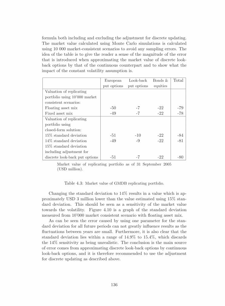
formula both including and excluding the adjustment for discrete updating.The market value calculated using Monte Carlo simulations is calculatedusing 10 000 market-consistent scenarios to avoid any sampling errors. Theidea of the table is to give the reader a sense of the magnitude of the errorthat is introduced when approximating the market value of discrete look-back options by that of the continuous counterpart and to show what theimpact of the constant volatility assumption is.
European Look-back Bonds & Totalput options put options equities
Valuation of replicatingportfolio using 10’000 marketconsistent scenarios:Floating asset mix -50 -7 -22 -79Fixed asset mix -49 -7 -22 -78Valuation of replicatingportfolio usingclosed-form solution:15% standard deviation -51 -10 -22 -8414% standard deviation -49 -9 -22 -8115% standard deviationincluding adjustment fordiscrete look-back put options -51 -7 -22 -80
Market value of replicating portfolio as of 31 September 2005(USD million).
Table 4.3: Market value of GMDB replicating portfolio.
Changing the standard deviation to 14% results in a value which is ap-proximately USD 3 million lower than the value estimated using 15% stan-dard deviation. This should be seen as a sensitivity of the market valuetowards the volatility. Figure 4.10 is a graph of the standard deviationmeasured from 10’000 market consistent scenario with floating asset mix.
As can be seen the error caused by using one parameter for the stan-dard deviation for all future periods can not greatly influence results as thefluctuations between years are small. Furthermore, it is also clear that thestandard deviation lies within a range of 14.9% to 15.4%, which discardsthe 14% sensitivity as being unrealistic. The conclusion is the main sourceof error comes from approximating discrete look-back options by continuouslook-back options, and it is therefore recommended to use the adjustmentfor discrete updating as described above.
136

Graph of the standard deviation measured from 10’000 market consistentscenario with floating asset mix.
Figure 4.10: GMDB scenario with floating asset mix.
137

5
Dependency Structure of theLife & Health Insurance Riskwith the Non-Life InsuranceRisks
It is important to clarify the dependency structure between the non-life andthe life-insurance risks in order to determine the group SST-target capital.
We have to consider fluctuation risks within L&H only when assessingthis dependency, as the trend risks are assumed to have no dependency toany other risk category.
The dependency structure between asset and credit and Non-Life risksimplies an indirect dependency between Life and Non-Life risks, but thediscussion of the method to determine this relationship is outside the scopeof this section.
A tail dependency between non-life and the life-insurance risk categoriescould arise if major events affect both life and non-life treaties negatively.
As such events have been very rare and the current historical data mostlikely do not reflect the occurrence of such events adequately, we use anapproach involving scenario techniques and copulas to reflect dependenciesbetween these risk categories:
1. We determine a list of possible events which could influence both lifeand non-life treaties substantially. This is a collaborative effort ofL&H and Non-life experts and is based on the Risk and Exposurestudy which lists all relevant such events.
2. We determine scenarios, covering these events and their range of im-pact adequately, assessing the probability using actuarial judgementand underwriting-know-how.
138

3. We evaluate the impact of these scenarios on L&H and Non-Life.
4. The marginal distributions without those events of the Life and Non-Life insurance risks are assumed to be given and independent.
5. A Monte Carlo simulation is used to combine the distributions witheach other and with the extreme scenarios (see the section on fluctu-ation risk, p. 111, for a detailed description of this approach) to getan empiric distribution of the combined risk.
6. A Clayton copula between the non-life and life risks is calibrated tothe result, reflecting the empirical dependency structure as far as pos-sible (see section on fluctuation risk for a detailed description of thisapproach).
7. This copula is then used to combine the marginal distributions of lifeand non-life risks (now we refer to the distributions including the ex-treme scenarios in a smoother way) (see section on fluctuation risk).
139

6
Mitigation of Insurance Risk
This section describes the risk (mitigation) modeling approach regarding in-surance risks that have been retroceded in the past (i.e. reinsurance assetsincluding the balances due from retrocessionaires for paid and unpaid lossesand loss expenses, ceded unearned premiums and ceded future life benefits1.)or are being retroceded in the current year. The credit risk due to thereinsurance assets is addressed in Part III (pp. 297) of this documentationunder the credit risk model (Muller [2007b]). Amounts recoverable from theretrocessionaires are estimated in a manner consistent with liabilities asso-ciated with the reinsurance contracts2. Our internal risk models treat thegross losses as stochastic variables modeled by line of business. Retrocededclaims from past business are modeled the same way as the gross reserves (seeChapter 3). Regarding retrocessions planned for the current year, we dif-ferentiate their modeling depending on the potential recovery amounts andcontract structure. Especially the cat retro structure is of major importancefor the risk mitigation of SCOR Switzerland (13% retroceded catastrophepremiums in 2007). Small recovery amounts and/or pure quota share retro-cession are modeled in a simplified way using regression techniques and/orthe corresponding fraction of the modeled gross loss. For large retrocessioncontracts the (individual) retroceded losses are modeled by applying the ex-plicit reinsurance contract structure on the individual gross losses. Hence,for these lines of business frequency-severity loss models are required. Theamounts to be recovered from retrocessionaires we call the retroceded lossesor recoveries, designated by Z, in order to distinguish them from the grosslosses which we denote by Z. In the following, both Z and Z are to beregarded as losses and recoveries by line of business, respectively3. So, for
1For the definition see Converium annual report 2006, p. 72.2Converium annual report 2006, p. 54.3The aggregation tool used for this purpose is Phobos, an IT component which allows
to collect the various lines of business into so called baskets. These baskets are organizedin a hierarchical tree of sub-portfolios and thereby reflect the dependency structure amongsub-portfolios which is central in the analysis of the liability model. In this section, line of
140

large standard excess of loss contracts for instance, individual recoveries Zi
are computed considering limits L, deductibles D and individual gross lossesZi via
Zi = min(L, max(0, Zi − D))
Regarding small recoveries the central assumption is that, for the pur-pose of stochastic simulations, the aggregate retroceded losses Z are linearlydependent on the aggregate gross losses Z via the equation
Z = α + βZ (6.1)
(How to take into account the fraction to be recovered from retroces-sionaires for small recoveries is outlined in a document by Michael Moller(Moller [2007]).) The parameters α and β we shall determine for each lineof business from the following data which, for each line of business, areassumed to be known beforehand.
� The retention δ defines the retroceded premiums P as a portion of thewritten premiums P
P = P (1 − δ)
� The retrocession loss ratio ν gives us the expected retroceded lossesE(Z) contingent on the retroceded premium P
E(Z) = νP
� The reinsurance risk loading κ is known together with the expectedretroceded losses E(Z) and the expected gross losses E(Z). This al-lows to express the standard deviation of retroceded losses σZ via thestandard deviation of gross losses σZ in the form
σZ = σZE(Z)E(Z)
+ κE(Z)
� The linear correlation of gross losses and retroceded losses is estimatedfrom past data4.
Corr(Z, Z) = h
business shall therefore mean a line of business as specified in Phobos. For more details onPhobos and other IT tools used for the SST process we refer to Part VIII, pp. 408. Therelevant SST process modules are described in the process landscape document, Skalskyand Burgi [2008], incorporated into this document as Part VII, pp. 353.
4Currently it is assumed by experts that the linear correlation is roughly about 0.7. Astatistical investigation for further backing this assumption will be done in short-term.
141

We compute the two parameters which govern the linear Equation (6.1)
β =σZ
σZCorr(Z, Z)
α = E(Z) − βE(Z)
142

7
Limitations of the LiabilityModel
7.1 Life Business
The main and most material limitation is the almost complete absence ofdata. This problem is most clearly visible
� For the main mortality risk driver pandemic
� For all trend risks
Furthermore it is obvious that given this lack of data for the marginals itis even less possible to reliably specify a dependency structure. This problemis not specific to the SCOR Switzerland Group but affects all (re)insurers.Likewise it cannot be solved by the SCOR Group on its own but poses ageneral challenge to any internal model.
In our specific internal model we tried to address those difficulties by
� Making very conservative (e.g. no diversification in trend risk)
� Relying on data provided by the regulator in the first place (FSAPpandemic scenario and trend risk distributions)
All other model limitations seem to be much smaller in comparison.
7.2 Non-Life Business
Limitations of the non-life liability model have been described implicitly inthe corresponding chapter. We mention here some of the main points.
With regards to the liability models constructed, we have separated thenew business and the run-off model. This is unsatisfactory in that new
143
choices

business written in the first year i = 0 becomes run-off business at t = 1,so the two models are not independent. Therefore, it would be preferableto have a consistent approach, combining new and run-off business in oneconsistent model.
In particular, concerning the portfolio dependency tree, it is unsatisfac-tory that the new and the run-off business dependency is formulated at thetop level. Especially for long-tail business, risk factors that impact the de-pendency between different contracts probably have an impact on both newas well as run-off business contracts. For this reason, new and run-off busi-ness for one type of business should probably be joined at a lower level inthe portfolio dependency tree.
Concerning the models of new and run-off business, the model for thenew business is considerably more sophisticated than the run-off businessmodel. This holds true for the dependency structure within the models aswell as for the respective basket models. We now address shortcomings ofthe two models separately.
7.2.1 New Business Model
To begin with, the new business model initially models nominal ultimateamounts. For the SST, however, models for the one-year changes are re-quired. Thus, we have to select proxies to derive one-year changes from ul-timate changes, and it would clearly be preferable to directly have a modelfor the one-year changes available. This applies both to the basket modelsas well as to the dependency structure in the portfolio dependency tree.
For the new business baskets, we use both default models (with implicitdependency structure) as well as basket-specific models. Ideally, default mod-els should be replaced as much as possible by basket-specific models, whichare explicit dependency models. However, very likely there will never bea specific model for every type of business. This because, first of all, therequired data for the contracts will often not be available (recall the re-quirements from Section 8.2.1, pp. 153), and, secondly, because there mightnot be (market-wide) data available to construct and parameterize such amodel. The most promising candidates for new basket-specific models cur-rently available are Aviation and Credit and Surety.
Another area for improvements is the default model itself. As described,the aggregation of the contract models to an (end) basket model is currentlyusing a one-parametric multidimensional Clayton copula with the propertythat the dependency structure is the same between any two contracts in thebasket. A potential improvement would be to use a copula family with morethan one parameter.
Considering improvements in the dependency structure, we mention thefollowing points:
� The structure of the portfolio dependency tree has to be updated.
144

� The values of the dependency parameters have to be reconsidered.
� The whole structure of the portfolio dependency tree is an implicitdependency model. It is desirable to try to work out at least qualita-tively the underlying explicit dependency model, i.e. to look for therisk factors causing the different types of dependencies. This could bedone directly or by creating a list of (realistic disaster) scenarios wheresuch (extremal) dependencies are manifested.
� It would be useful to classify dependencies. For instance, some de-pendencies arise while a contract is “under risk” (e.g. earthquakes,hurricanes, etc.), while others occur during run-off (e.g. legal changes).
7.2.2 Natural Catastrophe Modeling
This section is based on Pabst and Matter [2008].Revised (commercial and in-house) catastrophe models often lead to sig-
nificant changes in model outcome. Those changes reflect the uncertaintyand/or sensitivity of parameters mainly associated with the hazard and vul-nerability modules.
The understanding of the hazard’s mechanism and its mathematical rep-resentation are generally difficult for scientists. Major areas of research arefor instance the projection of future event probabilities from the past, andthus the completeness and comparability of data. An important aspect inhazard modeling is the correlation of hazards. (The occurrence probabilityof a severe loss amount increases with the consideration of collateral haz-ards.)
Usually, vulnerability functions for insured objects are derived from claimsdata and engineering analysis. They are often critical with respect to
� Regional specific reconstruction costs
� Representation of specific structure types
� Consideration of prevention measures (like dams)
The calibration of vulnerability functions is a process of continuous improve-ments and enhancements as more and more detailed descriptions and lossdata are available.
Exposure data are one of the model components where uncertainty canbe reduced most easily. Critical exposure data are mainly replacement value,construction type, occupancy type, and the geo-reference of the exposure.Significant data quality issues exist in particular for commercial property.
145

For multi-location policies the quality of the loss estimates depend stronglyon the description of each single location with regard to the assignment ofthe location limits and replacement values as well as the occupancy andbuilding type.
The today’s generation of catastrophe models focuses on exactly locat-able property values. Thus modeling business interruption and marine busi-ness remains challenging.
At present vendor catastrophe models do not take into account the accu-mulation of attritional losses for instance stemming from hail, thunderstormor torrential rain. Hence, models underestimate those loss components. Inaddition aggregate excess of loss contracts covering attritional losses cannotbe evaluated properly.
For the accumulation control or for pricing of individual contracts, wethus frequently apply adjustments to the models reflecting commercial struc-tures, non-modeled perils or collateral hazards.
Vendor models run the risk being biased by current market perspectivesnot necessarily reflecting scientific views.
Catastrophe modeling technology is not static and the models themselvescontinue to evolve in terms of detail, realism, and accuracy.
7.2.3 Run-off Business Model
Consider the run-off basket models as described in Section 3.9 (pp. 91).Unlike for new business, these models are already modeling the one-yearchange. However, for run-off business, no full distribution for the basketsis derived. Instead, only the expected value and the standard deviation arecalculated, and a distribution assumption (currently log-normal) has to bemade. In particular, the estimated standard deviation is used together withthe distribution assumption to estimate very small quantiles. It would bepreferable to derive the full distribution directly.
The method used to estimate the standard deviation for the one-yearchange is based on the Mack model assumptions. These, in particular, as-sume that the ultimate amounts in the triangle are calculated using thechain-ladder method. This is potentially unrealistic especially for the morerecent years, where the reserve estimates are often based on the pricing fig-ures or on a combination of the pricing figures and the triangles, such as theBornhutter-Ferguson method.
Further, the Mack method assumes that different underwriting years areindependent. This assumption is again questionable, as, especially for long-tail business, risk factors for one calendar year leading to notable reserveincreases for run-off business might reasonably have an impact on business
146

from all underwriting years at the same time. Thus, calendar year depen-dencies cannot currently be considered.
Finally, the dependency structure for run-off business should be recon-sidered, as the proposed structure was derived for new business, capturingultimate changes.
147
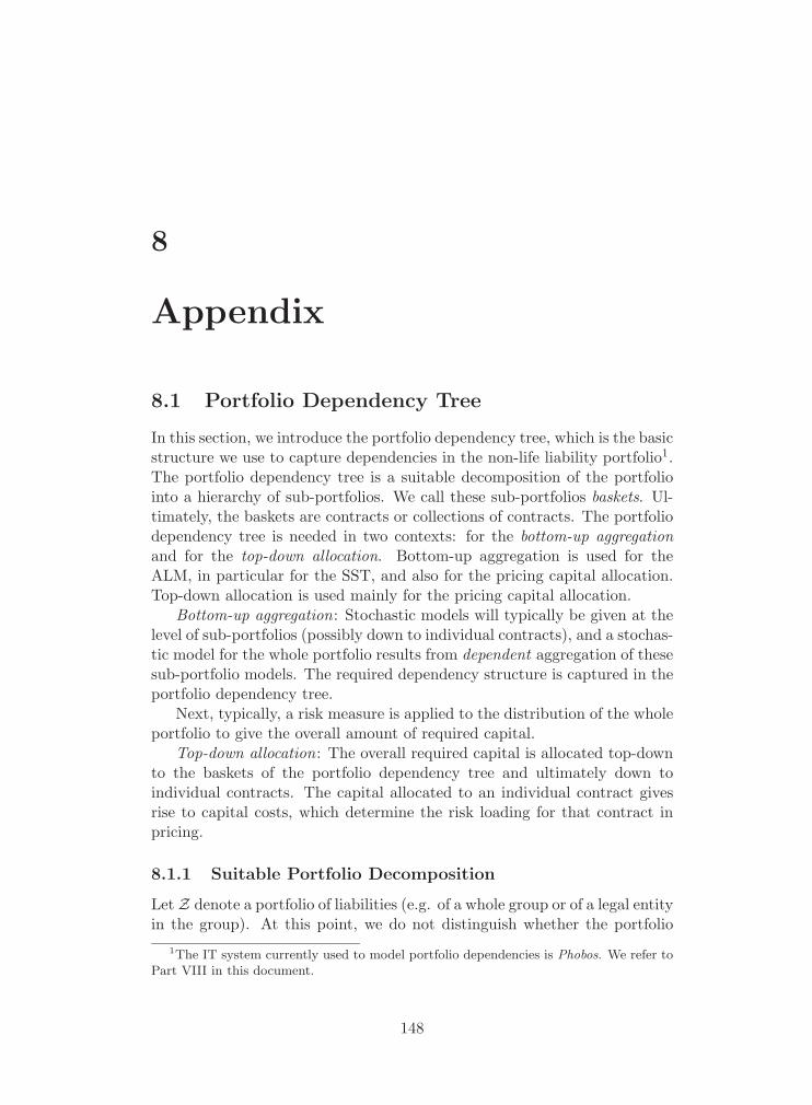
8
Appendix
8.1 Portfolio Dependency Tree
In this section, we introduce the portfolio dependency tree, which is the basicstructure we use to capture dependencies in the non-life liability portfolio1.The portfolio dependency tree is a suitable decomposition of the portfoliointo a hierarchy of sub-portfolios. We call these sub-portfolios baskets. Ul-timately, the baskets are contracts or collections of contracts. The portfoliodependency tree is needed in two contexts: for the bottom-up aggregationand for the top-down allocation. Bottom-up aggregation is used for theALM, in particular for the SST, and also for the pricing capital allocation.Top-down allocation is used mainly for the pricing capital allocation.
Bottom-up aggregation: Stochastic models will typically be given at thelevel of sub-portfolios (possibly down to individual contracts), and a stochas-tic model for the whole portfolio results from dependent aggregation of thesesub-portfolio models. The required dependency structure is captured in theportfolio dependency tree.
Next, typically, a risk measure is applied to the distribution of the wholeportfolio to give the overall amount of required capital.
Top-down allocation: The overall required capital is allocated top-downto the baskets of the portfolio dependency tree and ultimately down toindividual contracts. The capital allocated to an individual contract givesrise to capital costs, which determine the risk loading for that contract inpricing.
8.1.1 Suitable Portfolio Decomposition
Let Z denote a portfolio of liabilities (e.g. of a whole group or of a legal entityin the group). At this point, we do not distinguish whether the portfolio
1The IT system currently used to model portfolio dependencies is Phobos. We refer toPart VIII in this document.
148
contains new business or run-off business or both.To build a stochastic model for the portfolio Z, we inevitably need to
split the portfolio into suitable disjoint sub-portfolios, since stochastic mod-els will be available at the sub-portfolio level. We call the sub-portfolioswhich are not further decomposed the end baskets. These end baskets needto be suitably homogeneous for several reasons, see Section 3.2.
When aggregating the models of the sub-portfolios, dependencies be-tween the sub-portfolios need to be taken into account. Additionally, forpricing, as described in capital allocation (Section 8.3, pp. 168), we need amodel of the dependency of an individual contract to the whole portfolio.
If the number of sub-portfolios is large, and since any sub-portfolio mightdepend on any other sub-portfolio, the dependency structure might becomevery complicated. Moreover, as mentioned in Section 8.2, constructing high-dimensional dependency structures is not an easy task because constructingarbitrary high-dimensional copulas is not easy. For instance, assume that theportfolio consists of three end baskets, and that we specify the dependencybetween the first and the second basket, between the first and the third, andbetween the second and the third basket. Then, in general, there will notalways be a copula between the three baskets satisfying these specifications.
For this reason, the basic idea is to aggregate the end baskets by meansof a hierarchical dependency structure, and to use simple multidimensionalcopulas to express dependency within a hierarchy level.
Put differently, the portfolio is decomposed into disjoint sub-portfolios,some of which are further decomposed, etc. In this way we obtain a hierar-chical portfolio decomposition. We call sub-portfolios in this decompositionbaskets. So, in a first step, we decompose the portfolio Z into baskets
Z = Z1 + Z2 + · · · + Zn
Then, we further decompose some of the baskets Zi into baskets
Zi = Zi, 1 + Zi, 2 + · · · + Zi, ni
and so on.Recursively, we arrive at a hierarchical decomposition of Z, which we
view as a tree with root Z, see Table 8.1.To describe the tree structure, we introduce the following definitions:
Definition 8.1 The hierarchy level l of a basket is defined as the numberl of indices of the basket in the notation Zi1,··· ,il. The whole portfolio hashierarchy level 0. A basket X is called descendent of a basket Y in a givenportfolio decomposition, denoted
X � Y,
if X is a sub-portfolio of Y in this decomposition. A child is defined tobe a descendent in the portfolio tree of the next lower level, and a parent
149
Z
Z1
Z1,1
Z1,1,1 Z1,1,2
Z1,2 Z1,3
Z2 Z3
Z3,1 Z3.2
Hierarchical decomposition of Z into sub-portfolios.
Table 8.1: The portfolio dependency tree.
is defined analogously. Baskets that are not further decomposed into sub-portfolios (i.e. that have no descendents) are called end baskets of the tree.
Dependencies in the portfolio tree are always specified between childrenof a basket.
In order to ensure that the portfolio decomposition is applicable for ourpurposes, the decomposition needs to fulfill an additional condition we callsuitability. To define this condition, denote by X a random variable derivedfrom the cash flows of the sub-portfolio X (typically, the ultimate nominallosses or the net present value of the result) at a future point in time t,usually t = 1 or t = ∞.
Definition 8.2 A portfolio dependency tree of Z is defined to be a suitableportfolio decomposition, where a portfolio decomposition is called suitable ifthe following holds: Given baskets X � Y and a basket S which is not adescendent of Y, the random variables X and S are independent given Y ,that is, for any x, s, y ∈ R,
P[X ≤ x, S ≤ s | Y = y] = P[X ≤ x | Y = y] · P[S ≤ s | Y = y]. (8.1)
Equivalently, suitability can be expressed by
P[X ≤ x | S ≤ s, Y = y] = P[X ≤ x | Y = y]. (8.2)
8.1.2 Why Suitability is Needed
The property of suitability (8.1) is essential for two reasons:
1. In the bottom-up aggregation process, it allows to decentralize the mod-eling of certain baskets.
150
2. For the top-down allocation process, it enables a consistent risk allo-cation along the branches of the tree.
Regarding the first point, for a given basket, we would like to aggregatethe descendents of a basket without having to consider what happens atother parts of the dependency tree.
Regarding the second point, given baskets X � Y � S, we would likethat the dependency between X and S is determined by the dependencybetween X ,Y and between Y,S.
As an illustration of the first point, consider a basket S consisting of threebaskets X1, X2, and X3, so S = X1+X2+X3. Setting Y = X1+X2, we wouldlike to define the dependency between X1, X2, X3 by means of a hierarchicaltree structure. That is, we want the dependency between X1, X2, X3 to bedetermined by the dependency between X1, X2, and between Y, X3.
For this to work, we have to be able to derive the dependency between,e.g., X1 and X3 in term of the given dependencies. In fact, conditioning onY ,
P[X1 ≤ x1, X3 ≤ x3] =∫
P[X1 ≤ x1, X3 ≤ x3 | Y = y] dFY (y).
With no assumption on suitability, this can be rewritten
P[X1 ≤ x1, X3 ≤ x3] =
=∫
P[X1 ≤ x1 | Y = y, X3 ≤ x3] P[X3 ≤ x3 | Y = y] dFY (y).
Using suitability (8.2), the right hand side can be expressed in terms of thedependencies between X1, Y (i.e. between X1, X2) and between Y, X3, andsuitability is necessary for this to hold.
Further, an expression for the copula CX1,X2,X3 between X1, X2, X3 canbe derived as follows (see Section 8.2.2 for more on copulas). Using thedefinition of the copula CX1,X2,X3 and conditioning on Y ,
CX1,X2,X3(u1, u2, u3) = (8.3)
=∫ 1
0P
[X1 ≤ F−1
X1(u1), X2 ≤ F−1
X2(u2), X3 ≤ F−1
X3(u3) | Y = F−1
Y (v)]
dv.
Since Y = X1 + X2, we must have above that v is no larger than
v� ≡ v�(u1, u2) := FY (F−1X1
(u1) + F−1X2
(u2)), (8.4)
and provided this holds, the expression in the integral in (8.3) can be written
P
[F−1
Y (v) − F−1X2
(u2) < X1 ≤ F−1X1
(u1), X3 ≤ F−1X3
(u3) | Y = F−1Y (v)
].
151

To this probability, suitability (8.1) can be applied, and using that, e.g.,
P[X3 ≤ F−1X3
(u3) | Y = F−1Y (v)] = ∂1CY,X3(v, u3),
we finally get for the copula
CX1,X2,X3(u1, u2, u3) =
=∫ v�
0
(∂2CX1,Y (u1, v) − ∂2CX1,Y (FX1(F−1
Y (v) − F−1X2
(u2)), v))·
· ∂1CY,X3(v, u3) dv,
with v� = v�(u1, u2) as defined in (8.4). The expression in distribution func-tions and their inverse above evaluated is equal to 0 at v = 0, and equal tou1 at v�.
Concerning the second point, the top-down allocation process, the re-quirement expressed in terms of copulas is that, for a portfolio dependencytree with baskets X � Y � S, the copula CX,S can be calculated from thecopulas CX,Y and CY,S ; in fact,
CX,S = CX,Y � CY,S ,
where the composition of two copulas C1, C2 is defined as
(C1 � C2)(u, w) :=∫ 1
0∂2C1(u, v) ∂1C2(v, w) dv.
To show this, note that suitability implies that the random variables X andS are independent given Y . The claim then follows by conditioning on Y inthe equality
CX,S(u, w) = P[X ≤ F−1X (u), Z ≤ F−1
S (w)],
and using that, e.g.,
P[X ≤ F−1X (u) | Y = F−1
Y (v)] = ∂2CX,Y (u, v).
Because of the requirement of suitability, a portfolio decomposition needsto be selected with great care to ensure that we indeed get a portfolio de-pendency tree.
8.2 Modeling Dependencies
In this section, we first introduce the difference between explicit and im-plicit dependency models. We give a short introduction into copulas and
152

present different scalar measures of dependency measures including linearcorrelation, and sketch some of the well-known fallacies related to linearcorrelation. Next, we present the important family of Archimedean copulas,and its member the Clayton copula, which we use as a default assumptionin our models, see for instance in Section 3.3.2 (pp. 59) for the default newbusiness model.
Most of the contents of this section follow McNeil et al. [2005] and Nelsen[1999], where the proofs of most statements not given below can be found.
8.2.1 Explicit and Implicit Dependency Models
To begin with, we distinguish two different types of dependency models forrandom variables: explicit and implicit models. For implicit dependencymodels, dependency between random variables is expressed by specifyingthe dependency structure of the random variables directly, for instance by acorrelation matrix or, preferably, by a copula between the random variables.More details about copulas are provided in Section 8.2.2 below.
Explicit dependency models, on the other hand, are causal in the sensethat the underlying risk factors that are giving rise to dependencies areavailable as random variables, and the dependency between the given ran-dom variables is expressed through these risk factors. That is, given the riskfactors, the random variables are independent. The risk factors might againdepend on each other in an implicit fashion, or they might be independent.The model is explicit because the causes of the dependencies between thegiven random variables are modeled.
As an illustration, two random variables X and Y might depend ex-plicitly on each other through a common random variable θ in the sensethat
given θ, X and Y are independent.
Explicit dependency models are used, for instance, in the modeling ofnatural catastrophe contracts. More information about this can be found inthis document in Section 3.8 (pp. 80). The basic approach is the following:A natural catastrophe event is drawn stochastically out of an event catalogaccording to the event’s probability (e.g. an earthquake in a certain region,a certain tropical cyclone, etc.). The drawn event comes with its relevantspecifications (ideally, geographical distribution of the “severity” of the eventover time). The covered risks are specified by their geographical location(typically constant over time), their value, and their susceptibility to damagecaused by an event as a function of the event’s severity. The latter is usuallymeasured by so-called vulnerability functions and expresses loss or damagedegree, i.e. loss as a percentage of value. The relationship between eventintensity and loss degree in our models is usually stochastic.
The previous relationships provide the pre-insurance, or ground-up lossto the risk from the event. Applying the insurance structure to the pre-
153

insurance losses gives the insured losses, and applying the reinsurance struc-ture then gives the reinsured loss per contract and event.
In order to create an explicit dependency model for reinsurance con-tracts, we thus typically need
1. A multivariate distribution of the risk factors including dependencies(for instance, a collection of scenarios, that is, common samples of therisk factors with sample probability)
2. A collection of covered risks (“exposure information”),
3. A function (either deterministic or stochastic) assigning a pre-insuranceloss amount to a risk and a sample of risk factors,
4. The relevant insurance and reinsurance structures (as functions of thepre-insurance and insured loss, respectively).
In this case, dependencies between reinsurance contracts can come fromseveral sources (where below, dependencies mentioned early have an impactalso on the later ones):
� Dependencies between risk factors
� Dependencies between pre-insurance losses to different risks due totheir dependency on the same risk factors
� Dependencies between insured losses to different insurance policies dueto their covering the same risks
� Dependencies between reinsured losses to different reinsurance con-tracts due to their covering the same insurance policies.
In our non-life liability model, we use both implicit and explicit de-pendency models. In case no explicit dependency model is available, wecurrently use as default model an implicit model expressing dependency bymeans of a multidimensional, one-parametric Clayton copula. Argumentsfor this choice are given below in Section 8.2.4.
8.2.2 Copulas
In this section, we introduce the concept of copulas as a general approach tocapture dependencies between random variables, and list some of the mainproperties2.
2The Clayton copula, which is the Archimedean copula we currently use to modelimplicit dependencies (see 3.3.2, pp. 59) will be introduced in Section 8.2.4.
154
A natural approach to assess implicit dependency between random vari-ables is by means of rank vectors: Draw common samples from the randomvariables to get a collection of sample vectors. Assign each entry in a vectorits rank among the corresponding entries of the other sample vectors (e.g.the largest sample of the first random variable, the second largest sample ofthe third random variable, etc.) to obtain a collection of rank vectors. Forinstance, one rank vector might consist of the second largest sample of thefirst random variable together with the tenth largest sample of the secondrandom variable, etc. Plotting these rank vectors in a hypercube, we get anexample of a discrete copula. The density of points in a particular regionof the cube expresses dependency with respect to this region (for instance,whether large values of one random variable go together with large valuesof another random variable).
More formally, a d-dimensional copula
C : [0, 1]d → [0, 1]
is defined to be a distribution function on [0, 1]d with standard uniformmarginal distributions (margins).
To a copula C belongs a probability measure μ = μC on [0, 1]d such that
C(u1, . . . , ud) = μ([0, u1] × · · · × [0, ud]).
Explicitly, a function C : [0, 1]d → [0, 1] is a copula if and only if itsatisfies the following three criteria:
1. C(u1, . . . , ud) is increasing in each component uk
2. C(1, . . . , 1, uk, 1, . . . , 1) = uk for any k
3. The rectangle inequality holds: If μ is the probability measure be-longing to C, then the measure of any rectangle in [0, 1]d has to benon-negative. This condition can be expressed in terms of the functionC, which we do not explicitly give here.
For multivariate distributions, copulas are very useful because they allowto separate the dependency structure from the behavior of the univariatemargins. This is summarized in the following fundamental theorem of Sklar.
Theorem 8.3 (Sklar’s theorem): Let F be a distribution function with mar-gins F1 . . . Fd. Then, there exists a copula C : [0, 1]d → [0, 1] such that thefunction F can be written as
F (x1, . . . , xd) = C(F1(x1), . . . , Fd(xd)) for every −∞ ≤ xk ≤ ∞. (8.5)
The copula C is unique if the margins are continuous. Conversely, (8.5)defines a multivariate distribution function if F1 . . . Fd are univariate distri-bution functions and C is a copula.
155

Moreover, the copula C is given by
C(u1, . . . , ud) = F (F←1 (u1), . . . , F←d (ud)) for every 0 ≤ uk ≤ 1, (8.6)
where the generalized inverse G← of a distribution function G is defined by
G←(v) := inf{y | G(y) ≥ v}. (8.7)
Note that the copula is in general not unique if the margins are notcontinuous. For instance, if F has margins F1 and F2, where Fk has anatom at xk of weight dk > 0 for k = 1, 2 (i.e. Fk has a jump of size dk atxk), then the copula is not unique on the rectangle
[F1(x1), F1(x1) + d1] × [F2(x2), F2(x2) + d2],
and can, moreover, be arbitrarily chosen on the rectangle, provided thatthe projections to the sides of the rectangle are appropriately uniformlydistributed.
A crucial property of copulas is their invariance under strictly increas-ing transformations of the margins: If the random vector (X1, . . . , Xd) hascontinuous margins, and if T1, . . . , Td are strictly increasing functions, thenthe random vectors (X1, . . . , Xd) and (T1(X1), . . . , Td(Xd)) have the samecopula (given by (8.6)).
This statement is intuitively clear if we think of a copula as a collec-tion of rank vectors as sketched above: Since each of the transformationsTk is strictly increasing, the ranks of the samples of the random vectors(X1, . . . , Xd) and (T1(X1), . . . , Td(Xd)) are identical.
The copula corresponding to independent random variables is the inde-pendence copula Π given by
Π(u1, . . . , ud) =d∏
k=1
uk. (8.8)
Every d-dimensional copula C satisfies the following so-called Frechet-Hoeffding bounds
max
{d∑
k=1
uk + 1 − d, 0
}≤ C(u1, . . . , ud) ≤ min{u1, . . . , ud}. (8.9)
These bounds have interpretations in terms of dependency structures: Theupper bound on the right hand side above is assumed for the co-monotonicitycopula M and represents the dependency structure of perfectly dependentrandom variables. For d = 2, the lower bound above is assumed by thecounter-monotonicity copula W , representing perfect negative dependency;for d > 2, there is no copula assuming the lower bound.
156

Define the concordance order ≺ for copulas C1 and C2 by
C1 ≺ C2 if C1(u1, . . . , ud) ≤ C2(u1, . . . , ud) for all 0 ≤ uk ≤ 1. (8.10)
Then, the bounds (8.9) state that, for any 2-dimensional copula C,
W ≺ C ≺ M.
In the final part of this section we collect properties of copulas which aredesirable for our default dependency model. These properties put restric-tions on the possible types of copulas that should be considered for such adefault dependency model.
In our default basket model, we need to aggregate large numbers of con-tracts in one basket. To obtain a reasonably simple dependency model, itmakes sense to assume that, for the dependency structure, the contractsare exchangeable in the sense that it does not matter which contract isconsidered to be the first one, which one the second one etc. (Of course,exchangeability can be seen as a drawback, because the dependency struc-ture does not distinguish between components of the random vector. In ourportfolio dependency tree, however, this problem can be circumvented bycreating more baskets.)
Moreover, we would like not to have to recalculate the parameters forthe dependency structure when a new contract is added, and to ensure thatwe are consistent with the structure before adding the additional contract.These two requirements on the copula are reflected in the following twodefinitions.
A copula is called exchangeable if it is the copula of an exchangeablerandom vector X, where the latter means that, for any permutation π,
X ≡ (X1, . . . , Xd) is distributed like (Xπ(1), . . . , Xπ(d)),
so for the copula C,
C(u1, . . . , ud) = C(uπ(1), . . . , uπ(d)). (8.11)
A bivariate copula C is called associative if, for any u1, u2, u3 ∈ [0, 1],
C(u1, C(u2, u3) = C(C(u1, u2), u3). (8.12)
Associativity is closely related to Archimedean copulas, see Section 8.2.4.Archimedean copulas are, moreover, exchangeable.
For solvency considerations, we are primarily interested in evaluatingextreme occurrences, so we should focus on dependencies between extremeevents, that is, on the part of the copula describing such dependencies.Let’s assume that extreme events correspond to large negative values ofthe random variables. Then, for a bivariate random variable (X1, X2) with
157

continuous margins F1 and F2 and exchangeable copula C, define the lowerthreshold copula C0
ν for 0 < ν ≤ 1 as the copula describing the dependencyof X1 and X2 conditional on their both being below their ν-quantile. (Theupper threshold copula is defined analogously.) That is,
C0ν (u1, u2) =
C(F←(ν)(u1), F←(ν)(u2))
C(ν, ν)for u1, u2 ∈ [0, 1],
where G← denotes the generalized inverse of G as defined in (8.7), and F(ν)
is the conditional distribution
F(ν)(u) = P[X1 ≤ F←1 (u) | Aν ] =C(u, ν)C(ν, ν)
for 0 ≤ u ≤ ν
conditional on the event Aν of both X1 and X2 being below their ν-quantile,
Aν = {X1 ≤ F←1 (ν), X2 ≤ F←2 (ν)} .
It is then of interest to consider the limit of the copula C0ν as ν → 0. Such a
limit copula C is called limiting lower threshold copula, and needs to possessthe stability property that, for any 0 < ν ≤ 1,
C0ν (u1, u2) = C(u1, u2).
In particular, the Clayton copula used in the default model is such a limitinglower threshold copula, and it is an important attractor for a large class ofunderlying exchangeable copulas.
Lastly, it is convenient to work with a parameterized family of copulas.For parameterized copulas, we would like to be able to parameterize thefull range of dependency structures as expressed by the Frechet-Hoeffdingbounds (8.9), so the copula family should interpolate from the counter-W tothe co-monotonicity copula M , passing through the independence copula Π.Such a family of copulas is called comprehensive. The Clayton copula family(see below in Section 8.2.4) is comprehensive. Since we rarely encounternegative dependency, it would generally be sufficient to interpolate betweenindependence and co-monotonicity copula.
In case the copula family is one-parametric with parameter θ, we wouldlike the family of copulas to be positively (or negatively) ordered in the sensethat, for θ1 ≤ θ2 (or θ1 ≥ θ2), we have Cθ1 ≺ Cθ2 for the concordance orderdefined in (8.10).
8.2.3 Linear Correlation and other Dependency Measures
In this section we recall the definition of Pearson linear correlation, rankcorrelation, and coefficients of tail dependency. The main objective here isto have a scalar measure to express the nature of the dependency as cap-tured in the copula. Moreover, we recall limitations of these dependency
158

measures and, in particular, the fallacies connected with linear correlation.
The well-known linear correlation between two random variables X, Yis defined as
ρ(X, Y ) :=cov(X, Y )√
var(X) var(Y )∈ [−1, 1],
with
cov(X, Y ) = E[(X − E[X]) (Y − E[Y ])], var(X) = cov(X, X).
Linear correlation has the property that it is equal to 0 for independentrandom variables; the converse, however, is not true – a correlation of 0does not imply independence. A simple, rather extreme example is given bya normally distributed X and Y := X2: the correlation is zero although weclearly have a strong dependency.
A linear correlation of ±1 corresponds to perfect (positive or negative)linear dependency, meaning that Y = α + βX. Correlation is independentunder strictly increasing linear transformations – but not under arbitrarystrictly increasing non-linear transformations. The latter point is problem-atic because it implies (since copulas do have the full invariance property)that correlation cannot depend on the copula alone, but additionally alsodepends on the margins; consequently, correlation does not separate depen-dency structure from margins.
Another problem is that correlation is obviously only defined for randomvariables with finite variance, which might pose a problem for heavy-taileddistributions.
Next, we sketch three well-known fallacies related to linear correlation.They show that certain properties one would intuitively assume correlationto possess are in reality not fulfilled. The fallacies are discussed in moredetail, including explicit counterexamples, in Embrechts et al. [1999] and inMcNeil et al. [2005].
The first fallacy is that the joint distribution is uniquely determinedgiven the (continuous) marginal distributions and the pairwise correlations(uniqueness). The main point here is that it is in general possible to con-struct different copulas giving rise to different joint distributions havingthe same correlation. What is more, the V aR of a sum of dependent ran-dom variables is not uniquely determined from the marginal distributions ofthese random variables and their correlation matrix. The third fallacy belowpresents an additional pitfall when working with correlation and V aR.
The second fallacy is that, for given marginal distributions, it possibleto attain any correlation in [−1, 1] for a corresponding joint distribution(existence). In fact, using (8.9), one can show that the set of attainablecorrelations form a closed interval in [−1, 1] containing 0. Since a correlationof ±1 corresponds to perfect linear dependency as defined above, the intervalis, with the exception of the latter case, not the full interval [−1, 1].
159
The third fallacy pertains to correlation as well as to V aR. It states thatthe V aR of two risks is at its worst if the two risks have maximal correlation,i.e. if they are co-monotonic.
We focus now on scalar measures of dependency which only depend onthe copula and not on the margins: the two rank correlations Kendall’s tauand Spearman’s rho, and the coefficients of (upper and lower) tail depen-dency. From a practical point of view, they can be used to calibrate copulasto empirical data.
The rank correlation Kendall’s tau ρτ is defined as
ρτ (X, Y ) := E
[sign
((X − X) (Y − Y )
)]= 2 P[(X − X) (Y − Y ) > 0] − 1
= 4∫ 1
0
∫ 1
0C(u, v) dC(u, v) − 1 ∈ [−1, 1],
where (X, Y ) is an independent copy of (X, Y ), and the latter expressionshows that Kendall’s tau indeed only depends on the copula.
The rank correlation Spearman’s rho ρS is defined in terms of the linearcorrelation ρ by
ρS(X, Y ) := ρ(FX(X), FY (Y ))
= 12∫ 1
0
∫ 1
0(C(u, v) − u v) du dv ∈ [−1, 1].
The second fallacy above no longer applies to the two types of rank cor-relation as opposed to linear correlation. Clearly, the first fallacy remainsrelevant, which would be expected since one scalar should not be sufficientto fully specify a dependency structure.
Lastly, we consider the coefficients of tail dependency. These provide ameasure of extreme dependency: Given that one random variable takes anextreme value, what is the probability that the other random variable alsotakes an extreme value?
Indeed, for two random variables X and Y , the coefficient of lower taildependency λl, and the coefficient of upper tail dependency λu are definedas the limits
λl := limq→0+
P[X ≤ F←X (q) | Y ≤ F←Y (q)] = limq→0+
C(q, q)q
,
λu := limq→1−
P[X > F←X (q) | Y > F←Y (q)] = limq→0+
C(q, q)q
,
160

provided that the respective limits λl, λu ∈ [0, 1] exist, where the expressionsin terms of the copula hold for continuous margins. In the expression forthe upper tail dependency, C denotes the survival copula
C(u, v) = u + v − 1 + C(1 − u, 1 − v).
Two random variables are said to show upper (lower) tail dependency ifλu > 0 (λl > 0); otherwise, they are said to be asymptotically independentin the upper (lower) tail.
While tail dependency expresses dependency in the limit, it might makemore sense for practical purposes to study tail dependency at a certainquantile. We would then address questions such as: Given that one randomvariable is worse than its 1%-quantile, what is the probability that the otherrandom variable is also worse than its 1%-quantile?
To this end, we define the shifted (lower) tail dependency at the q-quantileTD(q) for q ∈ [0, 1] by
TD(q) := P[X ≤ F←X (q) | Y ≤ F←Y (q)] − P[X ≤ F←X (q)] =C(q, q)
q− q,
(8.13)where we shift the quotient to have TD(q) = 0 for independent randomvariables.
It is helpful, for a given copula, to study the function
h : (0, 1] → [0, 1], q → C(q, q)q
= P[X ≤ F←X (q) | Y ≤ F←Y (q)].
For q = 1, h takes the value h(1) = 1. As q moves to 0, h(q) convergesto the coefficient of lower tail dependency λl, provided the correspondinglimit exists. Plotting the function h from empirical data might thus givean indication of whether a certain dependency structure exhibits lower taildependency, and if so, what value the tail dependency might take. Also,studying the graph of h might give an indication of what kind of copulashould be used to model a certain dependency structure.
8.2.4 Archimedean Copulas, Clayton Copula
In this section we introduce the Clayton copula, which is the copula wecurrently use to model implicit dependencies, see for instance Section 3.3.2(pp. 59). The Clayton copula belongs to the class of Archimedean copulas.This latter class has a number of desirable properties, and we will highlightsome of them.
In particular, to model dependencies in our portfolio dependency tree,we need higher dimensional copulas. However, constructing copulas of di-mensions d > 2 is not easy, and might even be one of the main open problemsconcerning copulas. Recall to this end the three required properties (8.2.2) a
161

function C : [0, 1]d → [0, 1] has to fulfill in order to be a copula (in particular,the third property).
A naive approach to construct, e.g., three-dimensional copulas would beto couple two two-dimensional copulas C1 and C2 by defining
C(u1, u2, u3) := C2(C1(u1, u2), u3). (8.14)
Unfortunately, this procedure fails in general (see Nelsen [1999]). For in-stance, for the special copulas W, Π, and M , the formula (8.14) defines acopula in the following cases:
� If C1 = M , then C2 can be any copula, and if C2 = M , then C1 hasto be M .
� If C1 = W , then C2 has to be Π, and if C2 = W , then C1 has to beM .
� If C2 = Π, then C1 can be any copula.
These results already indicate that formula (8.14) will not most of the timeproduce a copula. However, in the class of Archimedean copulas, the proce-dure often succeeds.
One hint to construct Archimedean copulas of arbitrary dimensions comesfrom rewriting the independency copula Π from (8.8) as follows
Π(u1, . . . , ud) =d∏
k=1
uk = exp
(−
d∑k=1
(− log(uk))
).
Following this, let φ : [0, 1] → [0,∞] be a continuous, strictly decreasing,convex function with φ(1) = 0. We call φ an Archimedean copula generator,and strict if φ(0) = ∞. The pseudo-inverse φ[−1](t) at t ∈ [0,∞] is definedto be the usual inverse φ−1(t) for 0 ≤ t ≤ φ(0) and 0 otherwise. The idea isthen to define a d-dimensional copula Cd by
Cd(u1, . . . , ud) := φ[−1]
(d∑
k=1
φ(uk)
).
For dimension d = 2, this construction always succeeds. For higher dimen-sions d > 2, it succeeds for strict generators φ whose inverse f ≡ φ−1 iscompletely monotonic, that is,
(−1)k dk
dtkf(t) ≥ 0 for any k = 0, 1, 2 . . .
Any bivariate Archimedean copula C ≡ C2 satisfies the following alge-braic properties
162
1. C is symmetric, and thus also exchangeable as in (8.11). I.e., for anyu1, u2 ∈ [0, 1],
C(u1, u2) = C(u2, u1)
2. C is associative, as defined in (8.12)
3. for any u ∈ [0, 1],C(u, u) < u. (8.15)
Moreover, the latter two properties characterize Archimedean copulas: Anybivariate copula which is associative and satisfies (8.15) is Archimedean.
Regarding property (8.15), note that C(u, u) ≤ u always, and thatC(u, u) = 0 implies
P[X ≤ F←X (u) | Y ≤ F←Y (u)] = 1.
Recalling the proposed coupling construction (8.14), we have, for Archimedeancopulas with the same generator φ,
Cd(u1, . . . , ud) = C2(Cd−1(u1, . . . , ud−1), ud). (8.16)
Consequently, higher dimensional Archimedean copulas can be derived fromtheir bivariate counterparts by successive coupling.
An important family of Archimedean copulas are LT-Archimedean cop-ulas, whose generators are inverses of the Laplace-Stieltjes transform of adistribution function G on [0,∞) satisfying G(0) = 0; that is,
φ−1(t) =∫ ∞
0e−tx dG(x). (8.17)
An appealing aspect of LT-Archimedean copulas is the fact that they havean underlying explicit dependency model. Let V > 0 be a random vari-able. Denote its distribution function by G, and let φ be defined by (8.17).If the random variables U1, . . . , Ud on [0, 1] are independent given V withconditional distributions given V given by
P[Uk ≤ u | V = v] = exp(−v φ(u)) = (exp(−φ(u)))v ,
then the distribution function of the random vector (U1, . . . , Ud) is the LT-Archimedean copula with generator φ.
In particular, the dependency between the random variables U1, . . . , Ud
is explicitly given by the random variable V . Moreover, the above immedi-ately leads a procedure to sample from LT-Archimedean copulas by MonteCarlo methods.
163

The d-dimensional Clayton copula is an LT-Archimedean copula withone parameter θ given by
CCl(u1, . . . , ud) :=(u−θ
1 + · · · + u−θd
)−1/θ.
For d = 2, the parameter θ can take any value in [−1,∞) \ {0} with θ = −1giving W , θ → 0 equal to Π, and θ → ∞ giving M . For d > 2, we musthave θ > 0.
The bivariate Clayton copula has no upper tail dependency but lowertail dependency for θ > 0 with coefficient of lower tail dependency equal to
λl = 2−1/θ.
The generator φ of the Clayton copula is
φ(t) =1θ
(t−θ − 1
),
and the Clayton copula is an LT-Archimedean copula for a Gamma dis-tributed random variable V with
V ∼ Ga(1/θ, 1),
where the Gamma distribution Ga(α, β) for α, β > 0 has density
f(x) =βα
Γ(α)xα−1 exp(−β x).
We use the Clayton copula consistently as a default assumption in ourinternal model and in the capital allocation used for pricing to capture de-pendency between the children of a basket in the portfolio dependency tree.
In the following we summarize the desirable properties of the Claytoncopula family:
� It can be defined for arbitrary dimensions d.
� It is an LT-Archimedean copula, so there exists an underlying explicitdependency model, and it is easy to draw samples for Monte Carlosimulations.
� It is exchangeable and associative.
� Because of the property (8.16), if a random vector has a d-dimensionalClayton copula with parameter θ, the sub-random vector composed ofany two entries of the random vector is bivariate Clayton with thesame parameter θ.
164

� It is upper semi-comprehensive in that it allows to interpolate be-tween the independency copula Π (in the limit θ → 0+) and the co-monotonicity copula M (for θ → ∞).
� It is positively ordered3, i.e. for θ1 ≤ θ2, we have Cθ1 ≤ Cθ2 .
� It has lower tail dependency, which corresponds to the observationthat, in insurance and reinsurance, random variables are often almostindependent in normal situation but dependent in extreme situations(i.e. if it goes bad, then all contracts go bad).
� It is a natural choice to express dependency in extreme situations, sinceit is a limiting lower threshold copula: For a large class of copulas, thepart of the copula expressing dependency between extremes convergesto the Clayton copula (as shown by Juri and Wuthrich [2002]).
8.2.5 Explicit Dependency between Economic Variables andLiabilities
The stochastic liability model as explained in Section 3.2 offers full dis-tribution functions of aggregated claims. For some lines of business thesedistributions include economic risk factors. An example is Credit & Suretywhere the aggregated claim size is partially driven by the credit cycle, inaddition to idiosyncratic risk factors arising from individual treaties andinsured companies or securities. The stochastic liability model normallycovers all these risk factors, but there may be no technical way to separatethe influence of an economic variable from that of other risk factors.
Therefore economic risk factors are reintroduced in the internal modelin the form of an explicit dependency. Let the original loss be a stochasticvariable X from a distribution which originates from the liability model withmean X. In normal cases the distribution of X has a finite variance σ2
X .The economic risk factor Y usually comes from the Economic Scenario
Generator of the internal model. It describes the impact of the economicrisk factor on the specific liability with loss X and may be a function ofan economic variable rather than the variable itself. This function shouldbe chosen so that Y models the actual impact of the economic variable. Ifonly extreme values of the variable have an impact, for example, we choosea function with Y ≈ 0 for all average values of the economic variable and|Y | � 0 only for extreme variable values. In this example we shall observea tail dependency between the economic risk factor and the loss correctedby Y .
3This is proved in Nelsen [1999] for d = 2 and follows for higher dimensions d > 2 from(8.16) and the d = 2-case and component-wise monotonicity of copulas.
165

The two stochastic variables X and Y are independent as they originatefrom two entirely unrelated models. Mean Y and variance σ2
Y of Y areknown as they can easily be computed by the model simulation tool4. Theimpact of Y modifies the original loss X and leads to the corrected loss Z ina stochastic simulation. We always can and should define Y in a way thatits impact on Z is positive. This means that increases in X and in Y affectthe resulting corrected loss Z in the same positive direction.
For modeling the dependency we distinguish three cases with differentvalues of the additionality parameter α:
1. The distribution of losses X fully contains the impact of the risk factorY , so the only task is to make the hidden impact of Y on the lossesexplicit. The corrected loss has the same variance as the original one,σ2
Z = σ2X . This is the normal case. There is no additional risk, so
α = 0.
2. The distribution of losses X does not contain the impact of the riskfactor Y , possibly because that risk factor has been arbitrarily omittedin the calculation method of X. We mark the full additionality of thenew risk factor by setting α = 1. This is not the case in our currentliability modeling methodology, but here we offer a way to cover thecase of an additional risk factor, too.
3. The distribution of loss X partially contains the impact of the riskfactor Y . This case can be treated by choosing a parameter 0 < α <1. As in case 2, the corrected loss has a larger variance than theoriginal one, σ2
Z > σ2X .
In all the three cases the mean loss stays constant,
Z = X (8.18)
The dependency method never modifies the original loss expectation.The following explicit dependency model defines the corrected stochastic
loss Z of a simulation scenario as a linear combination of loss X and riskfactor Y :
Z = X + β (X − X) + γ (Y − Y ) (8.19)
This definition immediately satisfies Equation (8.18), whatever the valuesof the parameters β and γ. Both β and γ are positive or zero (in the caseof γ because we defined Y accordingly). The variance of Z is
σ2Z = β2 σ2
X + γ2 σ2Y (8.20)
4Currently the stochastic simulations are written in Igloo. For an overview of ITsystems and technologies, we refer the reader Part VIII in this documentation.
166

using the independence of X and Y . Using this independence again, we cancompute the linear correlation coefficient ρ between the risk factor Y andthe corrected loss Z:
ρ =γ σY
σZ=
γ σY√β2 σ2
X + γ2 σ2Y
In practice we choose ρ as the dependency parameter and use it to determinethe parameter values β and γ. Notice that ρ2 is the ratio between thevariance of the correction term γ(Y − Y ) and the variance of the correctedloss Z. Thus the new risk factor controls a share of ρ2 of the risk whereas theoriginal insurance risk of X keeps a share of 1−ρ2. In case of a considerablecorrelation of, say, ρ = 0.3, the new risk factor controls only 9% of the risk,and 91% of the original risk variance are maintained after the correction.In typical applications, ρ tends to be small as Y is just a minor economicrisk factor modifying a dominating insurance risk. Since we defined Y witha correct sign, ρ is confined between 0 (no impact of Y ) and 1 (where Yconverges to being the sole risk driver).
The parameters β and γ of Equation (8.19) can now be determined asfunctions of two more intuitive parameters, namely the additionality α andthe correlation ρ:
β =√
1 − ρ2 (1 − α) (8.21)
andγ = β
σX
σY
ρ√1 − ρ2
(8.22)
Reinsertion of β and γ in Equation (8.20) shows that the definitions lead toa variance with the desired properties:
σ2Z = σ2
X
1 − ρ2 (1 − α)1 − ρ2
In particular, the corrected variance σ2Z equals the original one, σ2
X , in thefrequently used case α = 0.
Let us summarize the procedure for obtaining a dependency model ofstochastic liabilities on an economic risk factor.
1. Confirm or correct the assumption α = 0. (The modeled risk factordoes not add any new risk, it just explains part of the already knownvariance.) Assess the correlation ρ between the economic risk factorand the total loss variance. Both parameter estimates, α and ρ, rely onthe (possibly model-based) input of experienced actuaries and otherexperts.
2. Use Equations (8.21) and (8.22) to compute the model parameters βand γ.
167
3. Use Equation (8.19) to compute the corrected loss Z in each trial ofthe stochastic simulation.
This dependency model offers a simple and efficient algorithm in theframework of a stochastic simulation. It avoids the introduction of indi-rect methods such as copulas and thus has the advantage of never creatingcircular or contradictory dependency conditions in complex models.
On the other hand there are possible weaknesses: (a) the additive modelof Equation (8.19) may cause negative losses in some cases, (b) the distri-bution of Z may differ from that of X even if they have the same mean andvariance and (c) the original dependency of X on other liability types is di-luted by a factor 1−ρ2. All these problems become negligible as long as theimpact of the risk factor is small, i.e. ρ2 � 1. As soon as the economic riskfactors start to dominate, we are using different modeling techniques, oneexample being our model for Guaranteed Minimum Death Benefit (GMDB)liabilities.
An important example for applying the dependency model of this sectionis the modeling of Credit & Surety losses. The credit level as explained inPart III takes the role of the risk factor Y in that case.
8.3 Pricing Capital Allocation
We describe the calculation of the sufficient premium for an insurance orreinsurance contract or policy implemented in the pricing tool. More pre-cisely, we describe the risk loading, which is based on capital (cost) alloca-tion, where the risk of the whole portfolio is measured by a spectral riskmeasure, which is currently the expected shortfall.
The allocated capital is calculated5 by general principles equivalent tothe Euler principle. Dependencies within the portfolio are modeled by meansof copulas in a hierarchical dependency structure we call the portfolio de-pendency tree. We derive expressions for the allocated capital in terms ofcopulas. The impact of diversification is expressed by the transformationof an initial risk function specifying the selected spectral risk measure intotransformed risk functions specifying the risk contribution of a sub-portfolioof the whole portfolio.
Further, the temporality of risk capital (the fact that risk capital is tieddown by a policy until there is no longer uncertainty about the outcome) isconsidered by means of a time factor measuring the duration of the policy.
In this way, the individual risk of a policy, the diversification with thewhole portfolio, and the duration of the policy are taken into account in thecalculation of the sufficient premium.
5For more details on the IT tools for pricing, dependency modeling and capital alloca-tion, we refer to Part VIII, pp. 408.
168

8.3.1 Introduction
It is well known that the required premium for an insurance or reinsurancepolicy or contract has to be larger than the sum of expected loss and ex-pected external and internal (i.e. administrative) expenses. The additionalamount can be considered as a risk loading, and to calculate it, actuarieshave traditionally used so called premium principles, such as expected lossprinciple or standard deviation principle.
For ease of notation, in the following, we take policy to mean eitherpolicy or contract.
Intuitively, when comparing the risk loading for different policies, therisk loading should have the following desirable properties: The risk loadingshould be larger
� The higher the risk (downside potential) of the policy
� The longer there is uncertainty about the final outcome
� The less the risk diversifies the overall portfolio of the (re)insurer
The most simple of the classical premium principles is the expected lossprinciple, where the risk loading is taken to be proportional to the expectedloss of the policy. The problem with this principle is, of course, that noneof the above desirable properties are satisfied. In particular, the risk (orvolatility) of the policy is not taken into account. Other premium principlessuch as the standard deviation principle or the exponential principle dotake the risk into account, but usually do not account for diversification.In addition, the standard deviation principle charges not just for downsidedeviations but also for upside deviations and, moreover, is not well suitedto reinsurance loss distributions which are often heavy tailed.
To overcome these shortcomings, one approach is to account for risk anddiversification in the above principles by the proportionality factor. That is,the portfolio is split into sub-portfolios, so that, within each sub-portfolio,the selected premium principle provides a reasonable measure. The resultingloading is then multiplied by a sub-portfolio specific proportionality factor.For instance, the sub-portfolios could be defined by line of business and typeof policy (e.g. for reinsurance treaties we could split into proportional andnon-proportional treaties).
Obviously, this approach – in theory – allows to account for all threedesirable properties above. It applies, more generally, to factor based mod-els. For instance, the risk loading could be calculated as the sum of a factorapplied to the premium plus another factor applied to the reserves, wherethe factors are specified by line of business and type of policy.
However, the approach has numerous drawbacks. To start with, it ishighly questionable that the required split into sub-portfolios is possible.As an example, for sub-portfolios composed of all policies of a certain line of
169
business and type of business, the expected loss principle will hardly be anadequate measure of the risk of all policies in a given sub-portfolio, so a muchfiner split would be needed. The problem of accounting for the desirableproperties is then transferred to the determination of the proportionalityfactors. Thus, a method is required to determine these factors correctly– how would such a quantitative method look like? This then raises thequestion of consistency : how can we ensure comparability of the risk loadingfor policies from different sub-portfolios? This is certainly desirable if wewant to have a true measure of expected profitability of policies, in order tobe able to optimize the overall net result of the portfolio.
More generally, in order to have a generic quantitative method to mea-sure profitability which guarantees comparability, it seems reasonable torequire that the method to calculate the risk loading rely as much as possi-ble only on the stochastic properties of the net cash flow of the policy overtime, and not on additional features of the policy.
We now formulate the idea of risk loading in a more economic way:Equity capital provided by the shareholders of the (re)insurance company isexposed to the risk that the actual result might be worse than the expectedresult, and for this reason investors expect a minimal annual spread abovethe risk free return on their investment.
This excess return gives rise to an overall annual capital cost amountcc(Z) to be earned by the whole portfolio Z of the (re)insurer. Given a riskX (a policy or a sub-portfolio) in the portfolio Z, the task of capital (cost)allocation is to determine the fraction of the overall capital costs that hasto be earned by the risk X . In the case of a policy X this fraction has tobe earned by the required premium of the policy in addition to the sum ofexpected loss and expected expenses.
Assume that the risk of the whole portfolio Z is measured by a riskmeasure ρ(Z) ∈ R. Denote by K(X ,Z) the contribution of the risk X tothe overall risk ρ(Z). Then it seems reasonable to allocate the capital costsproportionally to the risk contribution, i.e. the capital costs cc(X ) allocatedto X are given by
cc(X ) = cc(Z) · K(X ,Z)ρ(Z)
.
In particular, if we identify the risk ρ(Z) with the capital amount sup-porting the portfolio Z on which the required return η has to be earned, i.e.if cc(Z) = η · ρ(Z), we get
cc(X ) = η · K(X ,Z),
that is, the capital costs to be earned by X are given by the required returnη applied to the risk contribution.
We denote by temporality of risk capital the fact that the totalcapital for a policy X has to be set aside at inception of the policy and can
170
be gradually reduced as more information reduces the uncertainty aboutthe final outcome of the policy. However, some fraction of the capital is tieddown until the ultimate outcome of the policy is known.
In order to capture temporality of risk capital we need a model for thereduction of uncertainty over time. We choose as a proxy the incurred (orreported) pattern, which measures the fraction of ultimate losses that isincurred, i.e. known, up to some point in time. From this, we calculate atime factor τX for a policy X , which measures the duration of the policy.Incorporating temporality of risk capital, the capital costs to be earned byX are given by
cc(X ) = η · τX · K(X ,Z).
In our model, we use as risk measure the expected shortfall at a givenquantile, applied to the net present value of the result
premium − losses − expenses,
where future cash flows are discounted using the risk free yield curve for thecorresponding currency, and the respective maturity of the cash flows.
In other words, the risk measure is given by the average of the discountedworst outcomes, weighted with the probabilities of each of these outcomes.The selected quantile for the expected shortfall expresses the risk toleranceof the company.
Note that we deliberately apply the risk measure to the net presentvalue of the result as a random variable and not to the losses. Thisis important for instance for reinsurance contracts, where the premiumscharged and the expenses paid to the reinsured often are loss sensitive:Higher losses lead to higher premiums and/or lower expenses. Examples ofthis are sliding scale and profit commissions, reinstatements etc. This losssensitivity of premiums and expenses leads to a reduction of the volatility ofthe result of the contract, and would not be taken into account if we wouldonly consider the losses. In addition, the loss sensitivity of premiums andlosses is often non-linear (e.g. for reinstatements).
Given the risk measure expected shortfall, we use the Euler principleto calculate the risk contribution of a risk to the whole portfolio. That is,K(X, Z) is defined as the directional derivative of the risk measure ρ at thewhole portfolio Z in the direction of the risk X .
There are various justifications for calculating the risk contribution bythe Euler principle. Tasche [2000] argues by means of portfolio steering/performance measurement: The risk contribution should be calculated insuch a way that it rewards policies with a positive contribution to the overallresult, and punishes policies with a negative contribution. Denault [2001]uses cooperative game theory: The allocation of the overall capital coststo the policies has to be fair, which means that no coalition, i.e. no sub-portfolio of policies, would be better off on their own (i.e. the allocation isin the core of the cooperative game).
171

Further approaches to capital allocation include Kalkbrener [2005], wherean axiomatic approach to capital allocation is used, formulating desirableproperties. Another very general approach to capital allocation using dif-ferent methods is found in Denneberg and Maass [2006].
Note that the capital allocation methodology takes the risk of a policyinto account as well as the dependency between the outcome of the policyand the outcome of the whole portfolio. Thus, diversification is taken intoaccount.
For this reason, the method requires that we model the net present valueof the result of the whole portfolio and its dependency with the net presentvalue of each policy. To do this we need a method to aggregate risk inthe portfolio taking into account the dependencies between the risks. Thisaggregation of the portfolio is done in Phobos. It is also used to modelthe new business in the liability part for the SST and described in thecorresponding SST documentation.
8.3.2 Preliminaries
To begin with, we fix some notation. We denote by Z the portfolio underconsideration. The letters S,X ,Y are used to describe sub-portfolios ofZ. Usually, X refers to policies, and Y to portfolios of lines of businesses.Note that these variables stand for financial instruments. Monetary amountscorresponding to these financial instruments are in general random variables.In particular, we denote by Z, S, X, and Y the random variables of thecorresponding net present values of the result
premium − losses − expenses
The present values of future cash flows are always discounted using the riskfree yield curves of the corresponding currency, and the respective maturityof the cash flows. The random variables are defined on a suitable probabilityspace with probability measure P. By definition, bad outcomes correspondto large negative amounts.
For a random variable X we denote by FX its distribution function
FX : R → [0, 1], x → P[X ≤ x],
and by F−1X : [0, 1] → R the “inverse” q → inf{x ∈ R |FX(x) ≥ q}. For
simplicity, we assume, unless stated otherwise, that the random variablesunder consideration are continuous and strictly increasing.
In this article we are not considering how to model losses and expenses,and for this reason we always assume that the random variable losses-expenses is given for any risk we consider. In other words, we assume implic-itly that we have a stochastic model for losses and expenses. However, wedeal with the question of how to set the premium for a risk X in the portfolioZ, or, more precisely, the premium as a function of losses and expenses.
172

8.3.3 Risk Measure, Capital Allocation, Euler Principle, RiskFunction
In this section we describe capital allocation in the axiomatic framework ofKalkbrener [2005] and the extension of this approach to spectral measures ofrisk due to Overbeck [2004]. Very similar results, using a different approach,have been derived by Denneberg and Maass [2006]. As a special case ofspectral risk measures, we consider the expected shortfall.
For spectral risk measures there does not seem to exist a systematic in-vestigation of when the Euler principle holds, i.e. when the capital allocationis given by the directional derivative of the risk measure. Below, we give aresult for a special case which should suffice for practical applications.
Finally, we express the formula for capital allocation in terms of thecopula between the whole portfolio and a risk in the portfolio. This permitsa representation of capital allocation in terms of the emphrisk function.
To start with, we recall the well-known definition of coherent risk mea-sure (see for instance Artzner et al. [1999]). A mapping ρ assigning a realnumber ρ(X) ∈ R to a random variable X is called a coherent measure ofrisk if the following conditions are satisfied
positive homogeneity: ρ(aX) = aρ(X) for a ≥ 0 (8.23)sub-additivity: ρ(X + Y ) ≤ ρ(X) + ρ(Y ) (8.24)monotonicity: ρ(X) ≥ ρ(Y ) if X ≤ Y (8.25)
translation invariance: ρ(X + a) = ρ(X) − a for a ∈ R (8.26)
An example of a coherent risk measure is the expected shortfall at safetylevel α,
ρ(X) = ESα(X) = − 1α
∫ α
0F−1
X (u) du,
where the random variable X describes, e.g., the net present value of theresult of a financial instrument, so bad outcomes correspond to large negativevalues of X, and a high risk is a large positive number ρ(X). Unlike theexpected shortfall, the value at risk, V aRα(X) = −F−1
X (α), is not a coherentrisk measure, since it is in general not sub-additive, so it does not alwaysaccount for diversification.
The property (8.23) of positive homogeneity has been criticized since, forinstance, for large values of a, liquidity risk may arise. As an alternative,Follmer and Schied [2002] define convex measures of risk by replacing in theabove the properties (8.23) and (8.24) by
convexity: ρ(aX + (1 − a)Y ) ≤ aρ(X) + (1 − a)ρ(Y ) for 0 ≤ a ≤ 1.
Using the notion of risk measures we can now describe capital allocation.Consider the company’s portfolio Z, and decompose it into disjoint risks
173
(Xi)i=1,...,m, so for the net present values,∑Xi = Z.
The portfolio Z is supported by some capital K = ρ(Z), where ρ is agiven risk measure. A minimum annual spread η over the risk free interestrate has to be generated on K. The problem of determining the premiumfor X is reduced to the problem of allocating the capital K to the risks Xi.
In this framework, the task of capital allocation is to find risk contribu-tions K(Xi, Z) such that ∑
K(Xi, Z) = ρ(Z).
We then say that the amount of capital K(Xi, Z) is allocated to the risk Xi.In the following we assume that the capital allocated to a risk Xi depends
only on this risk and not on the decomposition of the rest
Z − Xi =∑k =i
Xk.
Consequently, a capital allocation with respect to a risk measure ρ can beconsidered as a map
K : V × V → R, with K(X, X) = ρ(X) ∀X ∈ V,
where V is some linear subspace of the space of equivalence classes of realvalued random variables on the selected probability space.
Kalkbrener [2005] shows that, given a risk measure ρ : V → R which ispositively homogeneous and sub-additive, i.e.
ρ(a X) = aρ(X) ∀a ≥ 0, X ∈ V,
ρ(X + Y ) ≤ ρ(X) + ρ(Y ) ∀X, Y ∈ V,
there exists a capital allocation K : V × V → R which is linear and diversi-fying, i.e.
K(aX + bY, Z) = a K(X, Z) + bK(Y, Z) ∀a, b ∈ R, X, Y, Z ∈ V,
K(X, Y ) ≤ K(X, X) = ρ(X) ∀X, Y ∈ V.
Conversely, if a linear and diversifying capital allocation exists with respectto ρ, then ρ is positively homogeneous and sub-additive.
Moreover, if a linear and diversifying capital allocation K for ρ is con-tinuous at some point Z ∈ V , i.e.
lims→0
K(X, Z + sX) = K(X, Z) ∀X ∈ V, (8.27)
174

then K(·, Z) is given by the directional derivative
K(X, Z) = lims→0
ρ(Z + sX) − ρ(Z)s
∀X ∈ V.
In other words, the risk contribution K(X, Z) is given by the Euler principle.Kalkbrener (Kalkbrener [2005]) proves these results by considering, for
given Z ∈ V , sub-tangents gZ ∈ V ∗, where V ∗ denotes the dual space oflinear functions from V into R, satisfying
gZ(Z) = ρ(Z), gZ(X) ≤ ρ(X) ∀X ∈ V.
Existence of the sub-tangents can be proved using the Hahn-Banach the-orem, or using theorems on sub-gradients of convex functions. Providedthese sub-tangents gZ exist for any Z ∈ V , the capital allocation K(X, Z)is defined as
K(X, Z) := gZ(X) ∀X ∈ V. (8.28)
As shown by Overbeck [2004], the above results of Kalkbrener (Kalkbrener[2005]) can be applied to so called spectral risk measures. We formulate thisapproach in a way which will be useful for us later on.
First, consider the special case where the risk measure is given by theexpected shortfall,
ρ(Z) = ESα(Z) = − 1α
∫ α
0F−1
Z (u) du
= −∫ 1
0F−1
Z (u)h(α)0 (u) du (8.29)
= −E[Z · h(α)0 (FZ(Z))], (8.30)
whereh
(α)0 (u) =
1α
1{u≤α} (8.31)
with 1A denoting the indicator function of the set A.For continuous random variables,
ρ(Z) = ESα(Z) = −E[Z | Z ≤ F−1Z (α)].
According to Kalkbrener (Kalkbrener [2005]), the capital allocation K(X, Z) =Kα(X, Z) is given by (8.28) with
Kα(X, Z) := gZ(X) = −E[X ·h(α)0 (FZ(Z))] = −E[X | Z ≤ F−1
Z (α)], (8.32)
where the last equality again holds for continuous random variables only.For the extension of the approach to spectral risk measures, the idea is
to replace the function hα0 in (8.31) by a more general function h0. To this
end, leth0 : [0, 1] → R
175
be a bounded, monotonously decreasing function. Define the associated riskmeasure ρ by
ρ(Z) := −∫ 1
0F−1
Z (u)h0(u) du. (8.33)
The interpretation is that such a risk measure is given by a weighted mean,where the uth quantile of Z is weighted by h0(u). In the special case ofthe expected shortfall, the weight function h0(u) is given by (8.31), whichmeans that all uth quantiles with u ≤ α are weighted with 1/α, while allother quantiles get weight zero.
We can rewrite (8.33), using
h0(u) = h0(1) −∫ 1
0β h
(β)0 (u) dh0(β) (8.34)
and (8.29), and changing the order of integration, to get
ρ(Z) = −h0(1) E[Z] −∫ 1
0β ESβ(Z) dh0(β). (8.35)
Now define the candidate K(X, Z) for the capital allocation by
K(X, Z) := −E[X · h0(FZ(Z))]. (8.36)
Using (8.34) and (8.32), and switching expected value and integration, (8.36)can be rewritten as
K(X, Z) = −h0(1) E[X] −∫ 1
0β Kβ(X, Z) dh0(β). (8.37)
Since h0 is decreasing, −dh0(β) ≥ 0. Thus, from (8.35) and (8.37), usingthe corresponding properties of the expected shortfall and expected value, itthen follows that ρ is a positively homogeneous, sub-additive risk measure,and that K defines a linear, diversifying capital allocation for ρ. Note thath0 decreasing is needed to ensure sub-additivity of the risk measure and thediversification property of the capital allocation.
The remaining more difficult part is to show that the capital allocationK(X, Z) is continuous at Z ∈ V in the sense of (8.27), which implies byKalkbrener’s results (Kalkbrener [2005]) mentioned above that K(X, Z) isgiven by the Euler principle, i.e. by the directional derivative of the riskmeasure,
K(X, Z) = lims→0
ρ(Z + sX) − ρ(Z)s
.
In view of (8.36), it has to be proved that
lims→0
E[X · (h0(FZ+sX(Z + sX)) − h0(FZ(Z)))] = 0. (8.38)
176

The main technical problem here seems to be that the random variableFZ+sX(Z + sX) might have an atom at a point where h0 is discontinu-ous. Equation (8.38) has been checked under the following (non-necessary)assumptions:
Assumption 8.4 (Capital allocation by the Euler principle)
1. The random variable Z is continuous and strictly increasing.
2. The random variable X is continuous with existing first and secondmoment.
3. The function h0 : [0, 1] → R is decreasing, bounded, and continuous inall but finitely many points. In the discontinuity points, both left andright limits exist.
As a next step, we express the formula (8.36) using the copula C = CX,Z
between X and Z,
C : [0, 1] × [0, 1] → [0, 1], FX,Z(x, z) = C(FX(x), FZ(z)),
where FX,Z is the distribution function of (X, Z), and FX , FZ are themarginal distributions of X, Z, respectively.
To this end, define H0 to be the integral of h0,
H0(u) :=∫ u
0h0(t) dt for u ∈ [0, 1],
and assume additionally that
H0(1) = 1.
Using the copula C = CX,Z we get from (8.36) with the definition of theexpected value,
K(X, Z) = −∫
R2
x h0(FZ(z)) ∂x∂zC(FX(x), FZ(z)) dxdz. (8.39)
Integrating in (8.39) first with respect to x and collecting terms not depend-ing on z, we get
K(X, Z) = −∫
R
x ∂x(H ◦ FX)(x) dx, (8.40)
withH(u) :=
∫R
∂zC(u, FZ(z)) h0(FZ(z)) dz. (8.41)
Substituting FZ(z) in (8.41) by v,
H(u) = HX,Z(u) =∫ 1
0∂2CX,Z(u, v) dH0(v). (8.42)
Formulas (8.40) and (8.42) can be found in Theorem 5.2 in Denneberg andMaass [2006].
177
Definition 8.5 The composition C � H of a copula C with a functionH : [0, 1] → [0, 1] is defined by
(C � H)(u) :=∫ 1
0∂2C(u, v) dH(v). (8.43)
Lemma 8.6 Let C be a copula, and let H : [0, 1] → [0, 1] be a monotonouslyincreasing function satisfying
H(0) = 0, H(1) = 1. (8.44)
Then, the composition C � H is a monotonously increasing function
C � H : [0, 1] → [0, 1] with (C � H)(0) = 0, (C � H)(1) = 1.
Proof 8.7 (Proof.) Let U , V be uniformly distributed random variables on[0, 1] such that
C(u, v) = P[U ≤ u, V ≤ v].
Then, the function
u ∈ [0, 1] → ∂2C(u, v) = P[U ≤ u | V = v] ∈ [0, 1]
is increasing with ∂2C(0, v) = 0 and ∂2C(1, v) = 1 for any v ∈ [0, 1]. SinceH is increasing, we have dH(v) ≥ 0 for every u ∈ [0, 1], and using (8.44),the claim follows.
Then, we arrive at the following expression for the capital allocationK(X, Z) in terms of the copula between X and Z,
K(X, Z) = −∫
R
x d(HX,Z ◦ FX)(x), (8.45)
with HX,Z = CX,Z � H0. (8.46)
Moreover, substituting u in (8.33) by z := F−1Z (u), we obtain for the asso-
ciated risk measure
ρ(Z) = K(Z, Z) = −∫
R
z d(HZ,Z ◦ FZ)(z), (8.47)
forHZ,Z := H0,
and the Euler principle holds
K(X, Z) = lims→0
ρ(Z + sX) − ρ(Z)s
.
As an interpretation of these formulas, consider the risk measure ρ tobe represented by the function H0, which we can view as the initial risk
178
function. The impact of diversification, by considering a risk X as part of awhole portfolio Z, leads to a transformation of the initial risk function H0
by the copula CX,Z into a transformed risk function H = CX,Z � H0.Furthermore, the equation for the risk contribution if a risk X in a
portfolio Z from (8.45) can be rewritten by a change of variables to give
K(X, Z) = −∫ 1
0F−1
X (u) hX,Z(u) du, (8.48)
where hX,Z denotes the derivative of HX,Z , assuming it exists. In words,the risk contribution is calculated by “weighting” the quantiles F−1
X (u) withthe derivative hX,Z of the transformed risk function HX,Z .
Definition 8.8 A function
H : [0, 1] → [0, 1] with H(0) = 0, H(1) = 1
is called an admissible initial risk function if H is concave, increasing,and continuously differentiable in all but finitely many points, and in thosepoints, both left and right derivatives exist.
Consequently, the preceding formulas hold for any initial risk functionH0 which is admissible.
In the case where the risk measure is given by the expected shortfall atsafety level α, the derivative h
(α)0 of the initial risk function H
(α)0 is given by
(8.31),
h(α)0 (u) =
1α
1{u≤α},
and the transformed risk function from (8.46) becomes
H(α)X,Z(u) =
(CX,Z � H
(α)0
)(u) =
1α
CX,Z(u, α). (8.49)
In this special case, consider again formula (8.48)
K(X, Z) = −∫ 1
0F−1
X (u) h(α)X,Z(u) du, (8.50)
where h(α)X,Z denotes the derivative of H
(α)X,Z , that is, from (8.49),
h(α)X,Z(u) =
1α
∂1CX,Z(u, α) =1α
P[Z ≤ F−1Z (α) | X = F−1
X (u)]. (8.51)
As an interpretation of these formulas, recall that the risk measure expectedshortfall only considers those states ω ∈ Ω of the world in which the wholeportfolio distribution Z is worse than or equal to its α-quantile F−1
Z (α).Consider now the formula for the risk contribution K(X, Z) of one risk X
179
in the portfolio. According to (8.51), the weight of one particular quantileF−1
X (u) of X in the risk contribution formula (8.50) is then given by thenormalized probability of the shortfall condition Z ≤ F−1
Z (α) given that Xis equal to this quantile F−1
X (u).In particular, if X takes discrete values xk, we can write
K(X, Z) = −∑
k
xk P[Z ≤ F−1Z (α) | X = xk] P[X = xk],
so the weight of the value xk of X in the risk contribution is given by itsprobability to occur multiplied by its “contribution” to those states of theworld for which the whole portfolio is bad.
Similarly to formula (8.37), we can express the transformed risk functionHX,Z for initial risk function H0 with derivative h0 in terms of the trans-formed risk functions H
(β)X,Z for the initial risk function H
(β)0 of the expected
shortfall. In fact, applying partial integration to (8.46), and using (8.49),we get
HX,Z(u) = h0(1) u −∫ 1
0β H
(β)X,Z(u) dh0(β)). (8.52)
It follows from (8.52) for instance that the transformed risk function HX,Z
is concave if every transformed risk function H(β)X,Z(u) = CX,Z(u, β)/β is
concave.
8.3.4 Capital Allocation for a Portfolio Dependency Tree
As we describe in more detail in the documentation of the liability model,in order to capture the dependency structure of the whole portfolio Z, wedecompose the portfolio into disjoint sub-portfolios, which are in turn furtherdecomposed into sub-portfolios, etc. In this way we obtain a hierarchicaldecomposition of the portfolio, which we view as a tree with root Z and callthe portfolio dependency tree. This portfolio dependency tree is needed foraggregation of sub-portfolios in the decomposition and for allocating riskcapital along the branches of the tree.
Note that sub-portfolios here can be true sub-portfolios in the sense ofcontaining at least two policies, but can also be single policies. Sub-portfolioswhich are not single policies are also called baskets.
The goal is to express the formulas from the previous section in theframework of a portfolio dependency tree. In particular, given a sub-portfolioY which is “in between” a policy X and the whole portfolio Z (such as aline of business sub-portfolio), we would like to express the allocated capitalK(X, Z) in a way that separates the dependency between X and Y from thedependency between Y and Z. The resulting formula is (8.57) below, whichwe first prove for the risk measure expected shortfall and then generalize tospectral risk measures in the sense of the prior section.
180

In order to be able to decentralize the modeling of certain sub-portfoliosand to guarantee a consistent capital allocation along the branches of theportfolio dependency tree, the portfolio decomposition has to be suitable.To define suitability we need the following definition.
Definition 8.9 A sub-portfolio X is a descendent of a sub-portfolio Y in agiven portfolio decomposition, denoted
X � Y, (8.53)
if X is a sub-portfolio of Y in this decomposition. Moreover, a child isdefined to be a descendent in the portfolio tree of the next lower level, and aparent is defined analogously.
Definition 8.10 A portfolio dependency tree of Z is defined to be a suitableportfolio decomposition, where a portfolio decomposition is called suitable ifthe following holds: Given sub-portfolios X � Y and a sub-portfolio S whichis not a descendent of Y, the random variables X and S are independentgiven Y , that is,
P[X ≤ x, S ≤ s | Y = y] = P[X ≤ x | Y = y]·P[S ≤ s | Y = y] ∀x, s, y ∈ R.
In the present context, given X � Y � Z, suitability implies that therandom variables X and Z are independent given Y . Hence, conditioningon Y in the equality
CX,Z(u, w) = P[X ≤ F−1X (u), Z ≤ F−1
Z (w)],
and using that, e.g.,
P[X ≤ F−1X (u) | Y = F−1
Y (v)] = ∂2CX,Y (u, v),
we obtain, for a portfolio dependency tree and sub-portfolios X � Y � Z,
CX,Z = CX,Y � CY,Z , (8.54)
where the composition of two copulas C1, C2 is defined as
(C1 � C2)(u, w) :=∫ 1
0∂2C1(u, v) ∂1C2(v, w) dv.
One checks that the composition � is associative in the sense that, forH : [0, 1] → [0, 1],
(C1 � C2) � H = C1 � (C2 � H). (8.55)
Moreover, the comonotonicity copula CM is the neutral element with respectto the composition �, in the sense that, for any copula C and function H,
for CM (u, v) := min(u, v), C �CM = C = CM �C, CM �H = H. (8.56)
181
Now assume that H0 is an arbitrary admissible initial risk function defin-ing the associated risk measure according to (8.47), and denote its trans-formed risk functions by, e.g., HX,Z .
Given sub-portfolios X � Y � Z in a portfolio dependency tree, weclaim that
HX,Z = CX,Y � HY,Z . (8.57)
Here, � defines descendants according to definition (8.53).In fact, (8.57) is a consequence of (8.46), (8.54), and (8.55), because
HX,Z = CX,Z �H0 = (CX,Y �CY,Z)�H0 = CX,Y �(CY,Z �H0) = CX,Y �HY,Z .
Formula (8.57) is useful because, for the calculation of the allocated capitalK(X, Z), we can separate the dependency between Y and Z in the riskfunction HY,Z from the dependency between X and Y in the copula CX,Y .Moreover, we get a consistent step wise allocation of the risk capital alongthe dependency tree:
Remark 8.11 Allocation of risk capital along the portfolio dependency tree.
1. Start with the initial risk function H0 = HZ,Z .
2. Use the copula CY,Z between Z and a child Y of Z to derive the trans-formed risk function HY,Z for Y according to (8.57),
HY,Z = CY,Z � HZ,Z
3. Calculate the allocated capital K(Y, Z) by (8.45),
K(Y, Z) = −∫
R
x d(HY,Z ◦ FY )(x).
4. For a child X of Y, use HY,Z and the copula CX,Y to get HX,Z andthus K(X, Z), etc.
So, to calculate the allocated capital K(X, Z) for a sub-portfolio or singlepolicy X , where X � Y � Z for a portfolio dependency tree, we need
1. the risk function HY,Z
2. the copula CX,Y and
3. the distribution FX of the net present value of the result of XConsider now the situation when we are pricing a policy X in the portfo-
lio Z. In order to apply the method above, the problem is that we need thecopula CX,Y (or, alternatively, the risk function HX,Z) for every policy X .
182

This might be feasible in case an explicit model for the dependency struc-ture is given, but, in the general case, a simpler approximation might bedesirable. The approach we propose is the following: Instead of the copulaCX,Y we assume we are given the copula
CX0,Y
between Y and a very small policy X0 not contained in Y, which we call thedistinguished policy.
The above topic is related to what we call the volume effect: Since thepolicy X is in the portfolio Z, the dependency in HX,Z is between X andthe portfolio Z containing X . We can decide to write a bigger or smallershare on the policy X , and obviously, then, the size of X has an impact onthe dependency between X and the portfolio Z. In other words, denotingZs := Z + sX, we want that
1s
K(sX, Zs)
increases with s > 0.To describe the proposed approach, let X be a policy with parent bucket
Y � Z. Because of (8.57), K(X, Z) can be calculated from HY,Z and CX,Y .
Assumption 8.12 The size of a policy X with X � Y � Z has an impactonly on the dependency between X and Y, and not on the dependency betweenY and Z. (Thus, HY,Z is fixed.)
Now note that, for random variables S, T with copula CS,T , we have
CS,T (s, t) =∫ s
0∂1CS,T (r, t) dr =
∫ s
0P[T ≤ F−1
T (t) | S = F−1S (r)] dr,
which implies, setting S = X and T = Y + X, that
CX,Y +X(u, v) =∫ u
0∂1CX,Y
(r, FY (F−1
Y +X(v) − F−1X (r)
)dr.
In this formula, the dependency between the policy X and the portfolioincluding the policy has been removed from the copula on the right handside. Moreover, for s > 0 arbitrarily small, CX,Y = CsX,Y . Hence, it seemsreasonable to approximate
CX,Y ≈ CX0,Y ,
where X0 denotes the distinguished policy, which is a very small policy “notcontained” in Y. Therefore,
CX,Y +X(u, v) ≈∫ u
0∂1CX0,Y
(r, FY (F−1
Y +X(v) − F−1X (r)
)dr. (8.58)
To determine the copula CX,Y +X approximatively in an efficient way, wecalibrate it by its tail dependency at some point β ∈ (0, 1).
183
Definition 8.13 For a copula C, the tail dependency quantile TdQβ (forβ ∈ (0, 1)) is defined as
TdQβ :=C(β, β)
β− β. (8.59)
Since F−1Y +X(β) ≤ F−1
Y (β), and using (8.58), we can estimate C(β, β) =CX,Y +X(β, β) in (8.59) by
CX,Y +X(β, β) ≤∫ β
0∂1CX0,Y
(r, FY (F−1
Y (β) − F−1X (r)
)dr.
To calculate the tail dependency quantile numerically, given a decomposition0 = u0 < u1 < · · · < un = β of the interval [0, β], we decompose the aboveintegral into a sum of integrals∫ uj
uj−1
∂1CX0,Y
(t, FY (F−1
Y (β) − F−1X (r)
)dr,
which we approximate by upper and lower bounds
Z±j :=∫ uj
uj−1
∂1CX0,Y
(t, FY (F−1
Y (β) − F−1X (u±j )
)dr,
= CX0,Y
(uj , FY (F−1
Y (β) − F−1X (u±j )
)−CX0,Y
(uj−1, FY (F−1
Y (β) − F−1X (u±j )
),
where u+j := uj−1 and u−j := uj .
Formula (8.59) for TdQ is then approximated by
TdQ ≈ 12β
n∑j=1
(Z+j + Z−j ) − β.
This formula allows to determine a one-parametric copula approximatingCX,Y +X .
In conclusion, to calculate the capital K(X, Z) allocated to a policy Xwith X � Y � Z, taking into account the volume effect, we need
1. the risk function HY,Z
2. the copula CX0,Y between Y and the distinguished policy X0
3. the distribution function FY and
4. the distribution function FX of the net present value of the resultof X
184

8.3.5 Temporality of Capital, Capital Costs
Consider a policy X in the whole portfolio Z consisting of all policies writtenin a given underwriting year. For this policy we determine a measure forits “duration.” By duration, we do not mean here the time span until allcash flows related to the policy are paid. Instead, duration refers to the, ingeneral, shorter time the policy is “under risk” in the sense that uncertaintyremains about those cash flows. This is because, as soon as the preciseamounts of future cash flows are known, no risk remains. Economically,duration corresponds to the time span capital has to be put aside for therespective policy.
More precisely, what we are interested in here is the sequence of riskcapitals
K0, K1, K2, . . .
that have to be set aside for the policy X in the years i = 0, 1, 2 . . . afterinception. We then have to guarantee that, on the level of expected values,the corresponding capital costs can be provided on the risk capitals Ki bythe policy premium. Note that the required return on capital will be given.
A main issue here is what to do with excess premium, i.e. in case weget more premium than needed, how is this excess premium changing thesequence of risk capitals?
Recall that X denotes the net present value of the ultimate result
premium − losses − expenses.
Since Z consists of all policies written in a given underwriting year, andbecause we measure risk by the expected shortfall at safety level α, we wantto guarantee that, in the average worst α percent of the outcomes of thewhole underwriting year portfolio Z, we are able to fulfill our obligationsto the policyholders. This means that we have to set aside the “ultimate”capital amount
ρ(Z) =∑X in Z
K(X, Z)
at the beginning of the underwriting year under consideration. As informa-tion about the outcome of the policies increases (and as losses are paid),uncertainty decreases, which means that we can free up a certain amountof capital. Some fraction of the capital remains tied down until there is nouncertainty left.
Consequently, we have for the sequence of risk capitals of the policy X ,
K0 = K(X, Z) ≥ K1 ≥ K2 ≥ . . . ,
where the capital amount Ki is tied down by the policy X from t = i untilt = i + 1. On this capital, the return η has to be provided at t = i + 1, and
185

consequently, the total capital costs to be earned by the policy X are givenby ∑
i≥0
pv(t=i+1→t=0) (η Ki) , (8.60)
where pv denotes present value taken using the risk free yield curve of thecurrency and the appropriate maturity.
We can measure the reduction of uncertainty over time by the knowledgepattern (ζi)i with
ζi :=Ki
K0.
The knowledge pattern satisfies
1 = ζ0 ≥ ζ1 ≥ ζ2 ≥ . . . with limi→∞
ζi = 0.
A main question here, as mentioned before, is how to treat excess premium.That is, let π > 0 be an additional premium amount (for the same risk X ),which we suppose for simplicity is received in cash at t = 0. Then the riskcontribution K(X, Z) satisfies
K(X + π, Z + π) = K(X, Z) − π,
which suggests that the excess premium π can be used to reduce the requiredultimate capital. In view of Equation (8.60) for the capital costs, this furthersuggests that no “capital costs” need to be paid on the excess premium,unlike on the capital. While this holds for the year i = 0, as π would not beconsidered part of the capital at t = 0, for the following years i = 1, 2 . . . thisis not so clear since it might be argued that the excess premium becomescapital at t = 1 and thus has to contribute to the capital costs.
The question could be formulated as: Who owns the excess premium?We come back to this in the next section.
As a proxy for the reduced uncertainty at time t = i we use the incurred(or reported) pattern of that policy. That is, we approximate the knowledgepattern by
ζi ≈ ultimate losses − incurred losses up to start of year i
ultimate lossesfor i = 0, 1, 2 . . .
8.3.6 Sufficient premium, Performance excess, RAC, TRAC
In this section we apply the preceding analysis to the pricing of an individualpolicy and sub-portfolios of policies. We define the sufficient premium for agiven policy, and the performance excess for the policy, which is a monetaryamount measuring the profitability of the policy. Further, we introducenormalized measures RAC and TRAC of the required capital for a policy.
186

By slight abuse of language, we will in the following mean by a policy Xeither an individual policy or a sub-portfolio of policies in the whole portfolioZ.
As before, denote by X the net present value of the result
premium − losses − expenses.
Write KX = K(X, Z) for the capital allocated to X in Z.We call the premium for a policy X sufficient if the expected value of
the net present value of the result pays for the cost of capital allocated toX from (8.60), in particular, considering temporality of capital.
More precisely, the premium for a policy X is defined to be sufficient if
E[X] ≥∑i≥0
pv(t=i+1→t=0) (η Ki) , (8.61)
where pv denotes present value taken using the risk free yield curve of thecurrency and the appropriate maturity, and the hurdle rate η is the requiredannual return on capital (in the appropriate currency). The premium iscalled technical in the case of equality above.
We define the risk adjusted capital RACX = RAC(X, Z) to be the cap-ital KX allocated to a policy X in case the premium is technical, so in sucha case, (8.61) becomes
E[X] =∑i≥0
pv(t=i+1→t=0) (η RACi) , (8.62)
where RACi denotes the required capital for year i if the premium is tech-nical, and RAC0 = RACX .
The technical premium is the natural premium since it covers the ex-pected losses and, on the level of expected values, allows to pay out thecapital costs. In this sense, the technical premium can be said to be thatpart of the premium which without question belongs to the policy.
For this reason we define the knowledge pattern (ζi)i with respect to thecapital amounts required for the technical premium, so, for i ≥ 0,
ζi :=RACi
RAC0.
The time factor τX as a measure of the “duration” of the policy is thendefined by
τX :=∑i≥0
pv(t=i+1→t=0) (ζi · 1) ,
where 1 is the unit in the currency of the policy. Using the time factor, weget at the technical premium from (8.62) that
E[X] = η τX RACX . (8.63)
187

The time factor τX1+X2 of the sum of two policies X1, X2 is given bythe weighted sum
τX1+X2 =RACX1
RACX1 + RACX2
τX1 +RACX2
RACX1 + RACX2
τX2 . (8.64)
We now turn to the issue mentioned in the previous section on howto treat excess premium, i.e. an amount π > 0 of premium in excess ofthe technical premium. For simplicity we suppose the excess premium isreceived in cash at t = 0. The question is relevant when we want to measurethe resulting excess profit, which is done in terms of the performance excessto be defined below.
As mentioned before, the risk contribution KX = K(X, Z) satisfies
K(X + π, Z + π) = K(X, Z) − π,
which suggests that the additional premium π can be used to reduce therequired capital, implying that no capital costs need to be paid on the excesspremium.
The issue then boils down to the question: Who “owns” the excess pre-mium, the shareholder or the policy? This question has an impact on thecapital amounts Ki on which the required return η has to be earned. Thereare three possible approaches to this:
1. The full excess premium is considered capital from the end of yeari = 0. Then, the capital amounts Ki subject to capital costs become
K0 = RAC0 − π, K1 = RAC1, K2 = RAC2, . . .
2. The full excess premium is never subject to capital costs. Thus, weget
K0 = RAC0 − π, K1 = RAC1 − π, K2 = RAC2 − π, . . .
3. The portion of the excess premium not subject to capital costs isproportional to the knowledge pattern ζi. Thus,
Ki = RACi − ζi π = ζi (RACX − π) = ζi KX ,
where KX denotes the risk contribution at the premium given by the sumof the technical premium and the excess premium.
Our approach is the third option above6.6A justification for this approach can be given as follows: The starting point is to
suppose that the excess premium π > 0 is used to provide a higher return on capitalη than the required return η. The required return η RACi is provided disregarding the
188
So if the premium is technical, an excess premium π applied to (8.63)leads to
E[X] + π = η τX KX . (8.66)
As a consequence, we can reformulate the definition (8.61): The premiumfor a policy X is sufficient if
E[X] ≥ η τX KX . (8.67)
Notice that in (8.67) we deliberately do not write E[X]/KX ≥ η ·τX ; thatis, we do not express profitability in terms of the return on the allocatedcapital. The latter is not equivalent to (8.67) since KX could be zero ornegative.
Definition (8.67) of the sufficient premium can be expressed in terms ofthe expected value with regards to a distorted probability measure, provid-ing a link to the work of Denneberg (Denneberg [1989]), and Wang (Wang[1996]). From a theoretical point of view, this has the nice feature thatsufficiency is no longer expressed using a separation between the expectedresult and an additional “loading” quantity.
In fact, from (8.67) and (8.45), we find that the premium for X in theportfolio Z is sufficient if and only if∫
R
x d(G0X,Z ◦ FX)(x) ≥ 0 for G0
X,Z(u) := u + η τX HX,Z(u).
In order to get a probability measure G, we need limx→∞G(x) = 1, whichmeans that we have to divide above by 1+η τX . This then leads the following“premium principle” for a risk X :
The premium for the risk X is sufficient if and only if
EX,Z [X] :=∫
R
x dGX,Z(x) ≥ 0,
excess premium. Let πi be the part of the excess premium not subject to capital costs inyear i, and assume that π0 = π. Then πi allows to reduce the required capital in yeari to RACi − πi, and so a higher return ηi can be provided according to
ηi (RACi − πi) = η RACi. (8.65)
(This equation is valid for πi < RACi.) We now impose that the higher return ηi = η bethe same for all years i. Setting i = 0 in (8.65), we find that the return η is given by
η = ηRACX
RACX − π,
and using this information in (8.65) for i �= 0, we find that, for any i,
πi = πRACi
RAC0.
189
where the probability measure GX,Z is defined by
GX,Z(x) :=FX(x) + η τX HX,Z(FX(x))
1 + η τX.
This corresponds to a quantile based premium principle; however, in theabove set up, the distorted probabilities differ from policy to policy, anddepend on the overall portfolio Z! This has to be expected if the premiumprinciple is supposed to take into account diversification explicitly and notjust the stand-alone risk.
The profitability of a policy X is measured by the performance excessPE = PE(X, Z) ∈ R, which is defined as the constant amount by which thenet present value of the result can be reduced (positive PE) or has to beincreased (negative PE) so that the adjusted premium becomes technical.From (8.66), it follows that the performance excess PE solves the equation
E[X] − PE = η · τX · (KX + PE). (8.68)
Thus,
PE =E[X] − η τX KX
1 + η τX.
One checks that a given premium is sufficient if and only if the performanceexcess is non-negative.
The performance excess has the useful property of being additive: Theperformance excess of a portfolio of policies is equal to the sum of the per-formance excesses of the policies in the portfolio. This allows to assess inan easy way the profitability of a program composed of several contracts,or of a whole client relationship – some of the client’s policies might not beprofitable, but others are, and summing up the performance excesses of eachpolicy gives the performance excess of the client relationship. Additivity ofthe performance excess follows from (8.68) due to additivity of the expectedvalue E and the risk contribution KX , and the definition of the time factorof the sum X1 + X2 from (8.64).
The risk adjusted capital RACX = RAC(X, Z) was defined above, andcan be written as
RACX = KX + PE.
The time and risk adjusted capital TRACX = TRAC(X, Z) is definedby
TRACX := τX · RACX
While the capital KX can become zero or negative, RACX and TRACX arealways positive (unless X is constant), so they are more suited to calculatingreturn on capital than KX . Note also that
E[X] ≥ η · τX · KX ⇔ E[X] ≥ η · τX · RACX ,
190

which is a consequence of the fact that a given premium is sufficient if andonly if the performance excess is non-negative.
Finally, TRACX is related to the capital RAC3 = RAC3(X, Z) (in thenotation of the financial modeling team) given by
RAC3 := E[X] + KX ,
which results in the case of the risk measure expected shortfall if the shortfallis measured as the deviation from the expected net present value instead ofthe deviation from zero. In fact, we have
TRACX =τX
1 + η τXRAC3.
This equation follows by adding KX + PE to both sides of Equation (8.68)and using the definition of the involved quantities.
191

II
Market Risk
192
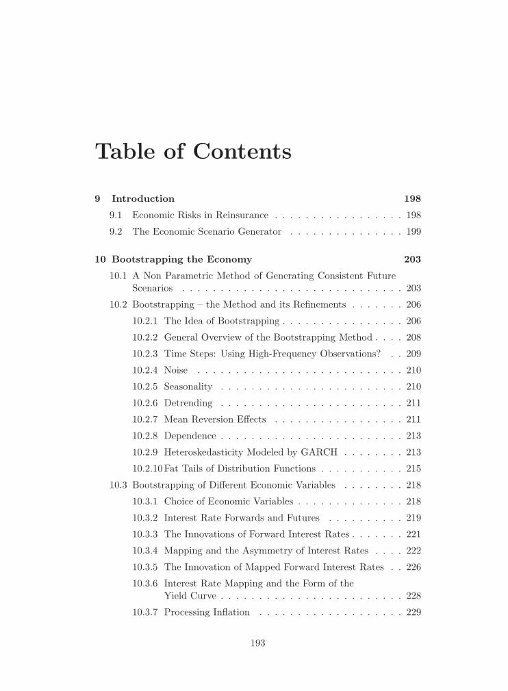
Table of Contents
9 Introduction 198
9.1 Economic Risks in Reinsurance . . . . . . . . . . . . . . . . . 198
9.2 The Economic Scenario Generator . . . . . . . . . . . . . . . 199
10 Bootstrapping the Economy 203
10.1 A Non Parametric Method of Generating Consistent FutureScenarios . . . . . . . . . . . . . . . . . . . . . . . . . . . . . 203
10.2 Bootstrapping – the Method and its Refinements . . . . . . . 206
10.2.1 The Idea of Bootstrapping . . . . . . . . . . . . . . . . 206
10.2.2 General Overview of the Bootstrapping Method . . . . 208
10.2.3 Time Steps: Using High-Frequency Observations? . . 209
10.2.4 Noise . . . . . . . . . . . . . . . . . . . . . . . . . . . 210
10.2.5 Seasonality . . . . . . . . . . . . . . . . . . . . . . . . 210
10.2.6 Detrending . . . . . . . . . . . . . . . . . . . . . . . . 211
10.2.7 Mean Reversion Effects . . . . . . . . . . . . . . . . . 211
10.2.8 Dependence . . . . . . . . . . . . . . . . . . . . . . . . 213
10.2.9 Heteroskedasticity Modeled by GARCH . . . . . . . . 213
10.2.10 Fat Tails of Distribution Functions . . . . . . . . . . . 215
10.3 Bootstrapping of Different Economic Variables . . . . . . . . 218
10.3.1 Choice of Economic Variables . . . . . . . . . . . . . . 218
10.3.2 Interest Rate Forwards and Futures . . . . . . . . . . 219
10.3.3 The Innovations of Forward Interest Rates . . . . . . . 221
10.3.4 Mapping and the Asymmetry of Interest Rates . . . . 222
10.3.5 The Innovation of Mapped Forward Interest Rates . . 226
10.3.6 Interest Rate Mapping and the Form of theYield Curve . . . . . . . . . . . . . . . . . . . . . . . . 228
10.3.7 Processing Inflation . . . . . . . . . . . . . . . . . . . 229
193

10.3.8 Interaction and Expectation of Interest Rates and In-flation . . . . . . . . . . . . . . . . . . . . . . . . . . . 230
10.3.9 Foreign Exchange Rates . . . . . . . . . . . . . . . . . 232
10.3.10 GDP . . . . . . . . . . . . . . . . . . . . . . . . . . . . 233
10.3.11 Equity Indices . . . . . . . . . . . . . . . . . . . . . . 234
10.4 Results and Testing . . . . . . . . . . . . . . . . . . . . . . . 235
10.4.1 Calibration . . . . . . . . . . . . . . . . . . . . . . . . 235
10.4.2 Example of Results: Yield Curve Simulation . . . . . 236
10.4.3 Out-of-Sample Backtesting . . . . . . . . . . . . . . . 237
10.5 Conclusion . . . . . . . . . . . . . . . . . . . . . . . . . . . . 242
10.6 Appendix: Robust Calibration of a GARCH Process . . . . . 243
11 Interest Rate Hedges 246
11.1 Swaptions . . . . . . . . . . . . . . . . . . . . . . . . . . . . . 247
11.2 Structured Notes . . . . . . . . . . . . . . . . . . . . . . . . . 247
11.3 Final Goal . . . . . . . . . . . . . . . . . . . . . . . . . . . . . 248
11.4 Sensitivity . . . . . . . . . . . . . . . . . . . . . . . . . . . . . 249
11.5 Valuation Formulae . . . . . . . . . . . . . . . . . . . . . . . . 249
11.5.1 Swaptions . . . . . . . . . . . . . . . . . . . . . . . . . 249
11.5.2 Notes . . . . . . . . . . . . . . . . . . . . . . . . . . . 250
12 Bond Portfolio Management 251
12.1 Introduction: Bonds, Equities, Cash . . . . . . . . . . . . . . 251
12.2 Bond Portfolios in Simulations . . . . . . . . . . . . . . . . . 252
12.3 Timing: The Simulation Period . . . . . . . . . . . . . . . . . 253
12.4 The Stylized Bond Portfolio . . . . . . . . . . . . . . . . . . . 254
12.5 Input Variables . . . . . . . . . . . . . . . . . . . . . . . . . . 255
12.6 The Bond Portfolio: Overview of the Algorithm . . . . . . . . 258
12.7 Initial Bond Portfolio Set-Up . . . . . . . . . . . . . . . . . . 258
12.8 The Bond Portfolio at the Midpoint of the Period . . . . . . . 260
12.9 Cash Flow from or to the Portfolio . . . . . . . . . . . . . . . 264
12.10 The Bond Portfolio at the End of the Period . . . . . . . . . 265
12.11 Accounting Results in Local Currency . . . . . . . . . . . . 266
12.12Final Accounting Results in Accounting Currency . . . . . . 275
12.13 Income Statement and Simulation Period Size . . . . . . . . 276
194

13 Accounting of an Equity Portfolio 277
13.1 Introduction . . . . . . . . . . . . . . . . . . . . . . . . . . . . 277
13.2 Timing: the Simulation Period . . . . . . . . . . . . . . . . . 277
13.3 The Equity Portfolio . . . . . . . . . . . . . . . . . . . . . . . 278
13.4 Input Variables . . . . . . . . . . . . . . . . . . . . . . . . . . 278
13.5 Cash Flow from or to the Portfolio . . . . . . . . . . . . . . . 280
13.6 Market Value Results . . . . . . . . . . . . . . . . . . . . . . 281
13.7 Accounting Results in Local Currency . . . . . . . . . . . . . 282
13.8 Final Accounting Results in Accounting Currency . . . . . . 284
13.9 Income Statement and Simulation Period Size . . . . . . . . . 286
14 Managing Cash Flows of Assets and Liabilities 287
14.1 Introduction . . . . . . . . . . . . . . . . . . . . . . . . . . . . 287
14.2 Timing: The Simulation Period . . . . . . . . . . . . . . . . . 288
14.3 Cash Flow from or to Liabilities . . . . . . . . . . . . . . . . . 288
14.4 Cash Flow from or to the Asset Components . . . . . . . . . 289
14.5 Cash Flow with a Hedging Component . . . . . . . . . . . . . 291
15 Foreign Exchange Risk 292
15.1 FX Risk and the Liability Model . . . . . . . . . . . . . . . . 292
15.2 Computation of Foreign Exchange Risk in our ALM Model . 292
16 Limitations of the Market Risk Model 295
195

List of Tables
12.1 Approximation for yields to maturity of bonds. . . . . . . . . . . 270
196

List of Figures
10.1 The bootstrapping method. . . . . . . . . . . . . . . . . . . . . 205
10.2 Interest rate mapping. . . . . . . . . . . . . . . . . . . . . . . . 224
10.3 Drift-free yield curves. . . . . . . . . . . . . . . . . . . . . . . . 228
10.4 Simulation of US yield curves. . . . . . . . . . . . . . . . . . . . 235
10.5 Out-of-sample backtesting. . . . . . . . . . . . . . . . . . . . . . 239
197
9
Introduction
9.1 Economic Risks in Reinsurance
In insurance risk models, liability risk is generally well examined and un-derstood. Investment risk, however, is often neglected or simplified1. To beable to assess these risks and their interaction SCOR Switzerland’s finan-cial modeling team has developed an economic scenario generator2 whichmakes predictions for a set of key risk factors in the most important eco-nomic zones. It provides realistic scenarios of possible future behaviors andconsistent estimates of risks in terms of both volatility and dependency.
The fortune and the risk of a business venture depends on the futurecourse of the economy. This is particularly true for the insurance and rein-surance industry. There is a strong demand for economic forecasts andscenarios that can be applied to planning and modeling. The main applica-tion of economic scenario generation is asset-liability management (ALM)3
in a reinsurance context which require models for all assets and liabilitiesof a firm and thus a comprehensive dynamic model for all economic vari-ables that determine asset and liability values. ALM requires forecastingeconomic development. By analyzing the risk exposure of the company,
1In this section we extensively quote from P. Blum, M. Dacorogna, U. Muller, A. Wallin,Using the past to predict economic risks, Helix brochure, Converium, August 2004, alsofrom M. Dacorogna, A. Wallin, Economic risks in reinsurance, Helix brochure, Converium,November 2004, and from the abstract and the introduction of (Muller et al. [2004])
2Economic scenario generation is a process step in the ALM and SST process. Werefer to the process landscape documentation, Part VII, pp. 353. The ESG itself is an ITsystem. For an overview of this system we refer to Part VIII.
3Central to the asset-liability management is the determination of the risk based capital(RBC) which is required to sustain a certain risk exposure. The capital intensity therebydetermined per line of business guides insurance business planning. The ALM and SSTprocesses are documented in Part VII. The ALM process optimizes the company’s overallrisk return profile. It thus comes into play for the investment risk side also throughstrategic asset allocation. The ALM process dynamically steers the company’s asset andliability portfolio. The entire ALM rests on a correct identification of all relevant riskfactors.
198

with an emphasis on the dynamics of invested assets, the company’s ALMprocess automatically provides the basis for the Swiss Solvency Test (SST).The SST demands from a company to assess the given risk exposure via thecalculation of the target capital (TC).
Invested assets are obviously contingent on the evolution of key eco-nomic or financial indicators such as yield curves, stock indices and foreignexchange rates and these also affect the performance of a reinsurer’s lia-bilities. SCOR Switzerland’s economic scenario generator is a concept tomodel and simulate the world economy (see also Part VIII in this docu-mentation). Within the ALM it enables to examine the various investmentstrategies and to predict their behavior. The large number of future eco-nomic scenarios finds its basis in the past known experience which allowsto predict the expected performance and risks of assets by reproducing thehistorically observed relationships between economic variables. The ESGexplicitly captures joint risks. The asset and liability risks are thus moreaccurately modeled, leading to more realistic investment strategies. The useof economic scenarios derived from historical market data combined with in-ternal risk models gives a more cautious picture of the investment portfolio’srisks. The method has several advantages. The use of historical observationsreduces the number of assumptions to be made. Any simultaneous depen-dence, such as between consumer price indices (CPI) and interest rates, arepreserved.
Certainly the future may hold surprises which have not been observedin the past or are otherwise not part of the data sample. As a partialcompensation for this lack of historical data the economic scenario gener-ator introduces tail corrections which provide for an additional stochasticvariability.
The methods behind the economic scenario generator (ESG) are docu-mented in Muller, Blum, Wallin, Bootstrapping the economy – a non para-metric method of generating consistent future scenarios (Muller et al. [2004]).
9.2 The Economic Scenario Generator
Scor Switzerland uses an economic scenario generator4 (ESG) to model therisks emanating from the financial markets. The stochastic model (Mulleret al. [2004]) behind the ESG allows to simulate the future development ofinterest rates (IR), gross domestic products (GDP) , foreign-currency ex-change rates (FX), consumer price indices (CPI), equity indices, hedge fundindices, real estate indices, mortgage based securities (MBS) and the creditrisk levels of entire currency zones (credit cycles). Historical time series ofeconomic indicators are collected, analyzed, adjusted and finally processed.The historical innovations are arranged into the future time series of inno-
4For IT systems in connection with the SST, see Part VIII in this documentation.
199

vations by means of statistical resampling. The notion of innovation empha-sizes the unanticipated movements that occur over time. An innovation isthe deviation of the value of a quantity from what was previously expected.The historical time series cover a time span of about ten years. For a typ-ical economic variable the innovations are calculated quarterly, resulting ina sample size of 40. The sample of innovations is thus indexed by around40 discrete time values. Due to the small size of this sample the model mustprovide for additional stochastic variation which it does in the form of oneadditional random variable, Pareto distributed, acting on each innovationas a weight factor.
Innovation events at different times are thought to occur independently.By contrast the innovations across the various variables which occur in paral-lel at a specified point in time epitomize the aspect of statistical dependence.The model preserves the dependencies between the variables. Arranging ascenario of future innovations means drawing from the sample of histori-cal innovations repeatedly. The method is bootstrapping : resampling withreplacement from the original sample. In each simulation step the ESG ran-domly selects among the forty available index times and thus specifies anentire vector of simultaneous innovations. These are concurrent innovationsin all the variables under consideration. Simultaneous dependencies amongthe economic quantities are therefore respected by this method.
At each simulated time step the simulated value of a variable is obtainedby adding up the simulated innovation with the market forecast. The boot-strapping step in simulations is done upon a transformation of the variablesin order to attain unlimited additivity of innovations. Stochastic trends areremoved beforehand. Mean reversion effects are understood as correctionsto the market forecast. The autoregressive behavior of the volatility of inno-vations is modeled by a GARCH process. To make the simulation of extremerisks realistic the resampled innovations are being weighted with a randomfactor. This will impose the desired heavy tail behavior to the probabilitydistributions of innovations, without changes to their variance.
Interest rates (IR) are modeled in terms of forward rates of IR futurecontracts. The model requires a non linear mapping and a soft bound onnegative rates. The mapping incorporates assumptions on the volatility atdifferent interest rate levels and on the mean reversion of interest rates whichfurther constrain long-term development of interest rate volatility.
Inflation is modeled using consumer price indices. Quarterly inflationnumbers are subject to a seasonal trend. The innovations are appropriatelydefined for deseasonalized and smoothed inflation data. The dependencebetween inflation and interest rates is in the form of an adjusted interestrate which is the difference between interest and inflation. Target inflationand target interest rates are proportional to the deviation of the adjustedinterest rate from its mean. Mean reversion is introduced to the model whenthese targets enter the formulation of market forecasts.
200
The model of foreign exchange rates (FX) is essentially specified by anassumption on how market expectations will be affected by the mutual de-viations of purchase power parities of different currency zones from eachother. A simplified approach transforms the FX scenarios into a stochasticmodel of the company’s overall FX risk (Dacorogna [2007a]).
For equity indices and gross domestic products (GDPs) the market expec-tation heavily relies on the latest attainable value together with the averagehistorical growth.
ESG simulations in the wider sense must be thought to comprise thegeneration of scenarios for variables not directly included in the economicscenario generator. Among these additional variables are option prices. Anystatistical sample originally drawn by the ESG will deterministically trans-late into a scenario for the price of an option via an option pricing formula.The ESG thus extends to novel variables. Scenarios for structured notes(Iannuzzi [2007]) and European look-back put options (Erixon and Kalberer[2005]) demonstrate the adequacy of the method.
ESG scenarios generally isolate the market risks. Nevertheless they affectthe study of the remaining components of risks which are interrelated. Asan example the credit cycles of currency zones are modeled like economicvariables in the ESG (Muller [2007b]). They express an overall level ofcredit risk inherent to the corporate bonds within a currency zone and thusconstitute an essential aspect of credit risk (Muller [2007b]).
Asset models like those for equity and bond portfolios (Muller [2006a],Muller [2007a]) clearly depend on the stochastic generation of economicscenarios (ESG). In our model, there is a very clear separation betweenthose modules which control the economic risks to which the assets areexposed (ESG), and those which mimic the policy of holding certain assets,like the bond portfolio management which is modeled separately (Muller[2007a]). On the side of liabilities, the economic scenario generator is noless essential: Yield curves, together with other variables, are needed in thevaluation (discounted best estimate) of future cash flows, therefore theseeconomic variables will inevitably appear in the liability model in the formof stochastic risk factors. A cash flow manager is then needed to accountfor the cash flows between assets and liabilities (Muller [2006c]).
The most prominent among the economic risks to which SCOR Switzer-land is exposed is interest rate risk. The stochastic economic scenario gen-eration therefore effectively translates to a stochstic model for the interestrate hedges (Iannuzzi [2007]) as these are composed of mainly swaptionsand structured notes whose valuation strictly depends on the risk factorsmodeled by the ESG.
Economic scenario generation, following a bootstrap approach, is laiddown in Muller et al. [2004]. This comprehensive paper follows a straightpath from the model’s overall principles to the concrete mathematical rela-tions which specify economic variables and their dependencies. It explains
201

the details needed in any concrete implementation of the model. The fol-lowing chapter will present, in a slightly adapted manner, the core sectionsof the bootstrapping paper (Muller et al. [2004]), a document that is clearlythe foundation on which other parts of the market risk model shall rest. Itallows for a reliable judgment on the level of accuracy and the consistencywith which the market risk is modeled at SCOR Switzerland.
202
10
Bootstrapping the Economy
10.1 A Non Parametric Method of Generating Con-sistent Future Scenarios
In this section, a concept to model and simulate the world economy is pre-sented. The economy is represented by a few key variables such as interestrates (yield curves), inflation, Gross Domestic Product (GDP) and equityindices, all of these for several currency zones, plus the foreign exchange(FX) rates between these zones. The goal is to generate scenarios that,in their entirety, represent the space of likely future developments. Thesescenarios can be used for simulating anything that depends on the economy.
Our main application is Asset-Liability Management (ALM) in a rein-surance context. ALM (see e.g. Ziemba and Mulvey [1998]) and DynamicFinancial Analysis (DFA, see Casualty Actuarial Society [1998] or Blum andDacorogna [2003]) require models for all assets and liabilities of a firm andthus a comprehensive, dynamic model for all economic variables that deter-mine asset and liability values. Our Economic Scenario Generator (ESG)has been developed to fulfill this requirement. Partial models for a restrictedset of economic variables cannot do this, no matter how sophisticated theyare, because of the complex dependencies between the variables.
Our method is bootstrapping, also called resampling. Initially, boot-strapping was a non-parametric method for limited tasks such as assessingconfidence limits of models estimated on finite data samples (Efron andTibshirani [1993]). Barone-Adesi et al. [1999] then applied bootstrappingto portfolio risk assessment, followed by Zenti and Pallotta [2000], Barone-Adesi et al. [2002] and Marsala et al. [2004]. The historical returns of certainassets became objects of resampling in simulations.
Bootstrapping constitutes the core of our model rather than being anadditional tool. Our basis is a set of historical time series of economic keyvariables. The returns or innovations of all economic variables as observed ina randomly selected historical time interval are taken and used for the simu-
203

lation of future time intervals. While there is an ongoing debate on modelingeconomic scenarios, the bootstrapping approach has several advantages. Itcan be implemented in a straightforward way and relies on past behaviors ofreal markets rather than debatable assumptions on models and parameters.Empirical distribution functions and simultaneous dependencies betweeneconomic variables are automatically captured. Bootstrapping belongs tothe family of non-parametric methods. Like other non-parametric models,our method still needs some parameters in order to define the method ina useful way, which ultimately makes the model semi-parametric. Anotheradvantage of bootstrapping is flexibility. We can easily add more economicvariables, which typically leads to large, comprehensive models.
Bootstrapping also has some disadvantages. Random trends may becontinued to the future indefinitely, serial correlations are disrupted by therandom selection of past intervals, and the statistical variety of behaviorsmay be too small in the historical time series, which implies that the proba-bility of extreme events may be underestimated. These problems are solvedby adding some preprocessing algorithms to the bootstrapping method. Thefollowing aspects have to be considered: choice and transformation of vari-ables, data frequency, dependence (serial and between variables), fat tails ofdistributions, the treatment of trends and mean reversion, and an arbitrage-free consistency of the resulting scenarios. Some of these refinements are notnew. Barone-Adesi et al. [1999] already found that some variables shouldpreferably be resampled in a mapped rather than raw form, so they de-veloped the method of filtered bootstrapping (Barone-Adesi et al. [2002];Marsala et al. [2004]; Zenti and Pallotta [2000]). This paper offers a wideset of bootstrapping refinements, based on economic principles and facts.These refinements eliminate the major pitfalls of bootstrapping and turnthis technique into a reliable generator of realistic scenarios.
A major difficulty for any parametric or non-parametric simulation modelis to determine reasonable expectations for economic variables such as in-flation or the growth of GDP or equity indices. Empirical means based onavailable samples of, say, ten years have stochastic errors or are biased bylong-term economic cycles. Long samples are not available in some cases(e.g. for the Euro, where synthetic data are needed). If they are available,they may be useless, such as foreign exchange data from before 1973, whencurrencies were under a different regime. Our ESG is based on historicaldata and naturally takes empirical means as expectations, but these can bemodified on the basis of expert opinion or special long-term studies such asDimson et al. [2003].
The quality of economic scenarios and forecasts based on bootstrap-ping has to be measured. Typical time horizons of economic scenarios aremeasured in years and quarters, so we have a limited number of historicalobservations that can be used for backtesting. An out-of-sample backtestingstudy based on a Probability Integral Transform (PIT) confirms the validity
204
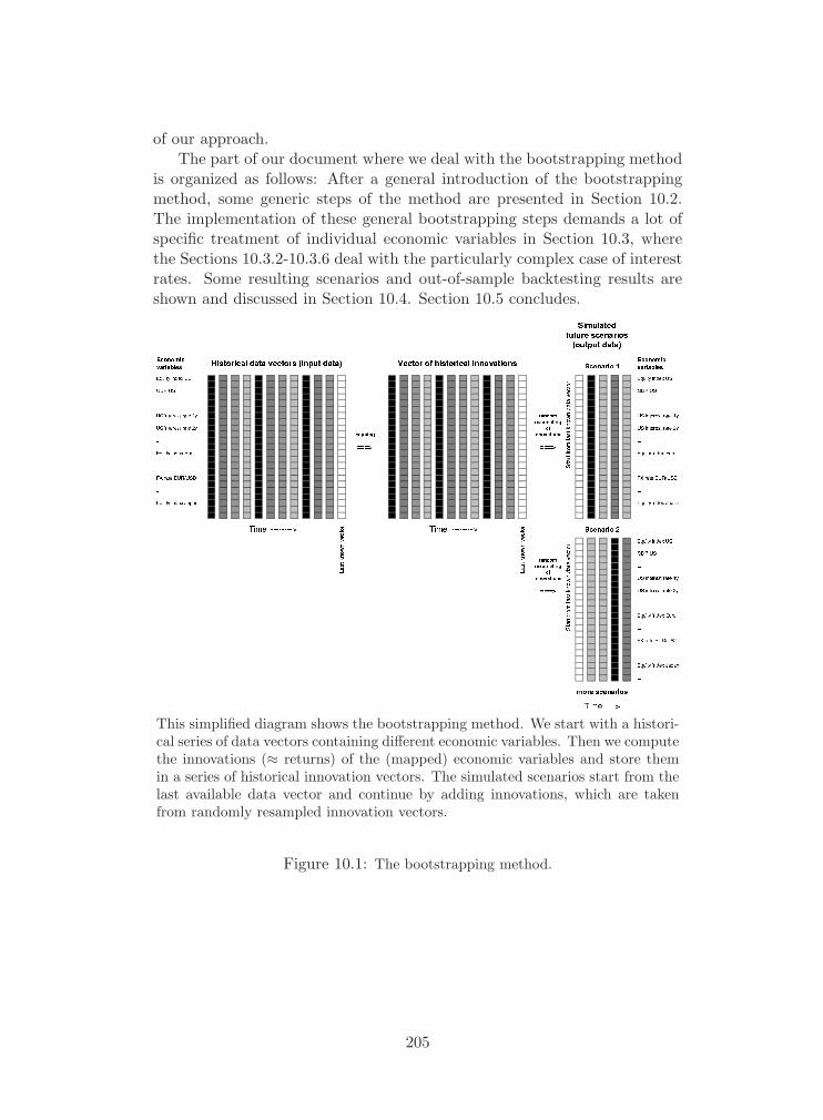
of our approach.The part of our document where we deal with the bootstrapping method
is organized as follows: After a general introduction of the bootstrappingmethod, some generic steps of the method are presented in Section 10.2.The implementation of these general bootstrapping steps demands a lot ofspecific treatment of individual economic variables in Section 10.3, wherethe Sections 10.3.2-10.3.6 deal with the particularly complex case of interestrates. Some resulting scenarios and out-of-sample backtesting results areshown and discussed in Section 10.4. Section 10.5 concludes.
This simplified diagram shows the bootstrapping method. We start with a histori-cal series of data vectors containing different economic variables. Then we computethe innovations (≈ returns) of the (mapped) economic variables and store themin a series of historical innovation vectors. The simulated scenarios start from thelast available data vector and continue by adding innovations, which are takenfrom randomly resampled innovation vectors.
Figure 10.1: The bootstrapping method.
205

10.2 Bootstrapping – the Method and its Refine-ments
10.2.1 The Idea of Bootstrapping
Our concept of bootstrapping is presented in Figure 10.1 in a schematic,simplified form. Before introducing methodological details or economic vari-ables, we discuss the bootstrapping method by means of a simple example.
We start from a sample of historical data, that is a set of time serieswith historical observations over a certain time period. There is a regular1
time sequence ti with time steps of size Δt:
ti = i Δt (10.1)
The corresponding time series values are Xi = X(ti) (e.g. an equity index)and Yi = Y (ti) (e.g. the GDP figures of the same country). The observationsof all the series are synchronous and cover the same historical period (e.g.the last ten years).
The last available values (the values now) are Xn and Yn. Our taskis to simulate future values at times t > tn: the vectors (Xn+1, Yn+1),(Xn+2, Yn+2), . . . , where the future values are in the same regular sequence,i.e. tn+k = (n + k)Δt. The basic idea of resampling is randomly picking anold time ti of the sample and assuming the same set of observations for afuture time of a scenario, e.g. for tn+1.
This is bootstrapping in its raw form, which will be modified in severalrespects. If we applied direct bootstrapping to the observations Xi and Yi,the simulated values would never leave the range given by historical values.A GDP figure could never grow to a yet unobserved value. Therefore, ourmain concept is to bootstrap innovations in economic variables rather thanthe variables themselves. These innovations will be resampled and added toold variable values at each simulation step in a cumulative way.
A simple definition of innovations might be first differences of variables.When cumulating randomly resampled first differences, the simulated vari-able may become negative, which is not appropriate for positive definiteeconomic variables. Returns are usually better than first differences. Loga-rithmic returns are an obvious choice. We can first transform the economicvariable by taking the logarithm and then take first differences. In the gen-eral case, we first introduce a variable transformation,
x(ti) = xi = F (Xi, Ii) = F [X(ti), I(ti)] (10.2)1While the method relies on regular historical input data for bootstrapping, an algo-
rithmic enhancement allows for starting a simulation from an irregular time point. Wedo not have to wait for the end of a quarter to produce up-to-date scenarios based onquarterly data.
206

where F can be a logarithm or a more complex function, which may dependnot only on Xi but also some simultaneous values of other economic variablessuch as Yi or, in general, the information set Ii available at time ti, whichincludes earlier values of the considered variables. The function F should beinvertible to determine X from x; its choice will be discussed for differentvariables. The innovation is defined in terms of xi rather than Xi, forexample as the first difference xi − xi−1. Most suitably, the innovation isdefined as the deviation of xi from its expectation2
Ei−1[xi] that the markethad at the previous time point ti−1:
Ii = xi − Ei−1[xi] (10.3)
The innovation Ii can be negative as well as positive. It constitutes theunanticipated element of surprise in a new value xi and is thus unrelated tothe market conditions at ti−1. In case of the martingale hypothesis, if theexpectation of xi made at ti−1 was xi−1, Ii would indeed be the first differ-ence of xi. In reality, the market often has a slightly different expectationEi−1[xi] at ti−1, so the innovation somewhat differs from the first difference.The market expectation Ei−1[xi] depends on the economic variable. For FXand interest rates, it is a forward rate. We agree with James and Webber[2000], Section 1.4.1, that forward rates are not particularly good predic-tors of spot rates, because the innovations Ii are large and unanticipated.Yet, an appropriate definition of Ei−1[xi] matters for long-term simulations,where seemingly weak modifications sum up to substantial effects. In Sec-tion 10.3, there are formulas for different economic variables, sometimesincluding some weak mean-reversion effects in Ei−1[xi].
The bootstrapping method will produce realistic results only if the Ii
values are independent over time and identically distributed (i.i.d.) withzero mean. It should be impossible to reject the i.i.d. hypothesis, given theempirical sample of historical innovations. Then the expectation of I2
i isindependent of current market conditions, in sufficient approximation. Themapping function F of Equation (10.2) has to be chosen accordingly. Thereis however the empirical phenomenon of volatility clustering which violatesthe independence of I2
i : a large I2i−1 tends to be followed by a large I2
i withincreased probability. In Section 10.2.9 this problem is solved.
In the course of simulation, the resampled innovations are used to modifythe simulated, future x values. For a future time tj , we randomly pick ahistorical index i and the innovation Ii of ti to obtain the new simulated
2Ei−1[xi] is used as a shortcut for the correct notation E[x(ti) | Ii−1].
207

value3:xj = Ej−1[xj ] + Ii (10.4)
This is an iteration. The next simulation time tj+1 will be treated thesame way, picking a new historical index i′ and re-using Equation (10.4) toobtain xj+1. After a few iterative simulation steps, the resulting x value willcontain an accumulation of many resampled innovations Ii. The variable xcan drift to any value and will not observe any range constraints. Mostoriginal economic variables Xi, on the other hand, are positive definite. Thelogarithmic function transforms a positive definite variable to an unlimitedreal variable and is thus a standard choice for the mapping function F ofEquation (10.2).
A main strength of the bootstrapping method is preservation of depen-dencies and correlations between variables. If the innovations Ii[x] and Ii[y](the corresponding innovation of the variable Yi) exhibit some dependencein the historical sample, the simulated variables xj and yj will be charac-terized by the same dependence structure. This is due to the fact that theresampled innovations Ii[x] and Ii[y] are always taken from the same his-torical time ti within a simulation step. The simulated mapped values xj
can be transformed back to standard values Xj by applying the functionF−1(., Ij) inverse to F (., Ij), see Equation (10.2).
10.2.2 General Overview of the Bootstrapping Method
An economically meaningful bootstrapping procedure requires a set of well-thought steps in addition to the simple bootstrapping principle as outlinedin the previous section. The general sequence of analysis steps is as follows:
� Start from a complete and representative sample of historical economictime series for several economic variables, regularly updated to thenewest values.
� Transform the economic variables (see Equation (10.2), sometimeswith deseasonalization, see Section 10.2.5), in order to attain unlimitedadditivity of innovations.
� Compute the market’s expectations of variables at each time ti−1 fortime ti (e.g. a forward rate as market predictor for a foreign exchangespot rate), including some weak, long-term mean-reversion effects.
3The first simulation step starts at the last regular time tj−1 = tn and leads to xj attime tj . Sometimes, there is information available at an irregular time tirreg after the lastregular historical time tn. In order to include this information in the first simulation step,the resampled innovation Ii can be modified to Imodified = Iirreg + [(tj − tirreg)/Δt]1/2Ii,where Iirreg is the historical innovation from tj−1 to tirreg.
208
� Compute the innovations of variables as the differences between thecurrent variable values and their previous market expectations, seeEquation (10.3).
� Remove stochastic trends by forcing a zero mean of innovations, toavoid arbitrary trends in later simulations, see Section 10.2.6.
� Treat autoregressive conditional heteroskedasticity (clusters of volatil-ity) of innovations by fitting a GARCH process, leading to GARCH-corrected innovations, see Section 10.2.9.
After this preparation, we are able to simulate future scenarios. We start byinitializing all the variables (including auxiliary ones) to the latest historicalvalues (the values now). The following sequence of steps describes one timestep into the simulated future, which can be iteratively repeated.
� Do the central bootstrapping step, taking a vector of past GARCH-corrected innovations, all from the same randomly picked historicaltime interval.
� Multiply all these innovations by a random tail correction factor, thusinjecting some rare shocks or stress scenarios that are not present inthe initial data sample.
� Re-transform the GARCH-corrected innovations to the actual innova-tions to be used, and update the GARCH volatility equation.
� Compute the simulated variable values as sums of previous marketexpectations and innovations, see Equation (10.4).
� Compute the market expectations of variables for the next simulationstep.
� Compute the simulated values of economic variables in their origi-nal definitions by doing transformations inverse to Equation (10.2)(reestablishing seasonality, if needed).
Notice that this sequence of steps mirrors the initially taken analysis stepsin reverse order.
This elaborated methodology applies to all economic variables, but thedetails of each step may look different for them. More details and problems ofthe method are described below. The special treatment of different economicvariables follows in Section 10.3.
10.2.3 Time Steps: Using High-Frequency Observations?
The size of the bootstrapping time steps depends on the application. Com-mercial simulation and planning tools may have yearly time steps, but the
209
generation of the underlying economic scenarios should be done in shortersteps. We can take quarterly steps and only use every fourth set of variablevalues, resulting in a yearly simulation.
When using a past of ten years, we have a basis of only 40 quarterly timeintervals. This is better than 10 (the number for using yearly steps), butstill rather low. A resampled year will consist of four quarters, each havingthe randomly selected innovations of a historical quarter. Thus there will bea wide variety in the behavior of simulated years: 404 (more than 2 million)possible sequences of quarterly innovations.
Of course, we can further increase the number of historical intervals bytaking monthly, weekly or daily time steps. For some variables such as GDP,high-frequency observations are not available. The clustering of volatilityhas been found to be stronger for high-frequency data in the literature,so the GARCH analysis (see Section 10.2.9) becomes more important. Inour actually implemented economic scenario generator, we are always usingquarterly time steps.
10.2.4 Noise
For some economic variables, the available data exhibit some noise. Herewe mean mean-reverting short-term noise rather than the natural volatilityof economic variables. Noise affects the innovation values computed byEquation (10.3) and leads to an increased variance of innovations. Thisincrease is spurious because it reflects mean-reverting movements ratherthan true drifts, so it may lead to a too high volatility of results simulatedover several time steps.
When using reliable data sources, this phenomenon is restricted to thosevariables whose definition is sensitive to such noise. In practice, this meansthe innovations of inflation and quarterly forward interest rates. The noisein consumer price index (CPI) figures is reinforced when computing inflation(a kind of first difference of the logarithmic CPI) and a second time whencomputing inflation innovations (which are similar to second differences ofthe logarithmic CPI). Quarterly forward interest rates have some almostinevitable noise due to small interpolation errors in the rather coarse gridof maturities supported by the yield curve data.
In these cases of noise, some smoothing techniques such as averaging arerecommended in order to avoid spurious volatility in simulation results.
10.2.5 Seasonality
A variable recorded in a time series is called seasonal if its values or its firstdifferences (or returns) have a seasonal pattern. This means that averagessampled at certain regular time intervals (e.g. second quarters of each year)
210

significantly deviate from averages sampled at shifted intervals (e.g. thirdquarters).
Prices in liquid markets such as FX, fixed income or equity hardly exhibitany significant seasonality, as empirical studies have shown. (Otherwise,these could be exploited in a systematic way.) Other financial variables suchas inflation and GDP may be seasonal as there is no investment strategy toexploit seasonality. Quarterly inflation rates (first differences of logarithmsof the CPI) indeed exhibit some seasonality aside from the noise discussedin Section 10.2.4.
In order to use a seasonal variable for bootstrapping, we have to desea-sonalize its historical observations before computing the innovations. Thesimulation results will be reseasonalized at the end. This is further discussedin Section 10.3.7.
10.2.6 Detrending
In our simulations, we use innovations according to Equation (10.4) in aniterative way, thereby cumulating the innovations. Innovations are definedas deviations from prior market forecasts. If the market forecasts are reason-able4, we expect a mixture of positive and negative innovations in the longrun, but the empirical mean of innovations within a historical sample mayslightly (stochastically) deviate from zero. In that case, we risk introducinga trend into the simulated future.
Generating such a trend is not justified even if it existed as a randomphenomenon in the historical data. Therefore we force the innovations tohave a zero mean:
Ii =√
n
n − 1
⎛⎝Iraw,i − 1
n
n∑j=1
Iraw,j
⎞⎠ (10.5)
Each raw innovation Iraw,i is corrected by subtracting the sample mean.When doing so, we implicitly minimize the variance of Ii about zero by usingone degree of freedom. Therefore we need the correction factor
√n/(n − 1)
to restore the expected variance of innovations. Equation (10.5) is used forthe correction of all innovations of the algorithm.
10.2.7 Mean Reversion Effects
When cumulating our detrended innovations, we obtain a stochastic randomwalk of the resulting variable, similar to a Brownian motion. Such motionsdo not exhibit any mean reversion. For most variables such as equity indices,
4This does not mean free of trends. Some economic variables such as equity indices orsome FX rates (Peso effect) have a natural trend that we have to model in the marketforecast.
211

this behavior conforms to theory and empirical findings. For other variablessuch as interest rates, however, there is a weak mean-reverting force whichmakes sure that interest rate levels do not drift to arbitrarily high (or low)values, even after decades and centuries. Another law with mean-revertingcharacter is purchasing-power parity (PPP). FX and inflation rates observethis law only hesitantly, with time lags of several years (see the article byCheung in Chan et al. [2000]).
In our bootstrapping algorithm, a natural place to implement the smallmean-reverting correction is the market forecast Ei−1[xi] of Equation (10.3).Mean reversion is a known phenomenon rather than an innovative surprise,so it belongs to the market forecast in the form of a small correction of thepurely technical market forecast. Although such corrections are small, theymay persist over years and exert a decisive force in real markets as well asin our simulations.
The mathematical nature of the small correction differs between eco-nomic variables and will be discussed in Section 10.3. In many cases ofmean reversion, we use varying target values rather than constant means.Some of these are moving averages. This can be implemented in the form ofan exponentially weighted moving average (EMA), which has the advantageof a very simple iteration formula for updating:
EMAi[x; Δtrange] = μ EMAi−1[x; Δtrange] + (1 − μ) xi (10.6)
withμ = e−Δt/T (10.7)
where xi stands for any variable to be averaged over time, and the timeconstant Δtrange is the range (= centre of gravity of the weighting kernel)of the EMA. There are more complex moving averages and iterations, seeDacorogna et al. [2001], but the simple mechanism of Equations (10.6) and(10.7) is certainly good enough to describe the behavior of means that areonly used to make weak corrections. At the beginning, each EMA has to beinitialized, using a sufficiently large sample of xi . We use the best estimatefor the EMA at the very beginning of the historical sample and iterativelyuse Equation (10.6) through the whole historical sample.
When modeling weak mean reversion, we stay simple and pragmatic, oth-erwise the method would become a full-fledged econometric modeling effortrather than remaining a bootstrapping algorithm. Mean-reversion effectsoften involve several variables with different volatility levels. In this case,we often prefer applying the mean-reversion correction to the high-volatilityvariable, where the low-volatility variable acts as a sort of dragging anchor.In the example of purchasing-power parity (PPP), the high-volatility FXrate is weakly anchored by the low-volatility consumer price indices (CPI)of the two currency zones.
212

10.2.8 Dependence
Simultaneous innovations in different time series often depend on each other.Equity indices in different countries, for example, rarely move in differentdirections. The bootstrapping method captures these dependencies verywell, as all innovations of a simulation step are resampled from the samehistorical time interval. Contemporaneous dependencies found in historicaldata are thus preserved.
Other forms of economic dependency pose some problems. Dependen-cies do not only exist for innovations, but also for the original and sim-ulated variables. This can often be described as a mean-reversion effectsuch as purchasing-power parity (PPP) and has already been discussed inSection 10.2.7.
Serial dependence of innovations would mean that new innovations arepartially anticipated by older ones. This is not the case here, since we defineinnovations as unpredictable in Equation (10.3).
If the serial dependence is in the volatility of an economic variablerather than the variable itself, we talk about autoregressive conditional het-eroskedasticity. This is treated in Section 10.2.9.
10.2.9 Heteroskedasticity Modeled by GARCH
Heteroskedasticity means a variation in the volatility of a variable over time.This is only a useful concept if a model for this volatility can be formulated.One way to model future volatility would be using implied volatility fromoption markets. For market variables such as FX, IR and equity indices,this is feasible as long as such volatility data are available (which is not thecase for the long time horizons of certain ALM studies). We do not pursuethis idea here.
Autoregressive conditional heteroskedasticity (clustering of volatility) isa well-known phenomenon (Baillie et al. [1996]; Bollerslev [1986]; Dacorognaet al. [2001]; Engle [1982]) in finance. For economic high-frequency datasuch as daily market prices, this is very significant. However, the effectis weaker for the data frequency of economic scenarios (such as quarterlyor yearly). We model the effect by approximately assuming a GARCH(1,1)process (Bollerslev [1986]). We fit a GARCH(1,1) process to the innovationsas computed from the raw data.
The GARCH(1,1) process for the observed innovations Ii is
Ii = σi εi , (10.8)
σ2i = α0 + α1 I2
i−1 + β1 σ2i−1
with three positive parameters α0, α1 and β1. The variable εi is iden-tically and independently distributed (i.i.d.), with mean 0 and variance 1.The GARCH process is stationary with finite variance if α1 + β1 < 1.
213
Calibrating the parameters of a GARCH process to the innovations Ii isnot a trivial routine task, although its feasibility with the help of commercialsoftware may lead a user to that assumption. The usual quasi-maximum-likelihood method poses some problems in practice, such as convergence tonon-stationary solutions (especially if the GARCH process is misspecified),local maximums of the likelihood function and other convergence problems.In some cases, Zumbach [2000] finds a maximum of the likelihood functionfor a GARCH process whose unconditional variance is about ten times theempirical variance of the data sample. The reasons are misspecificationand limited sample size. Zumbach [2000] even finds such effects for datagenerated by a GARCH(1,1) process. Finite sample sizes pose problems forGARCH fitting that tend to be underestimated in the literature.
Our historical innovation series based on low-frequency data definitelyconstitute small samples. Yet we need a reliable, robust GARCH calibra-tion algorithm for the repeated analysis of dozens of economic variableswithout any human intervention. We warn against a careless use of stan-dard GARCH fitting method. Our robust GARCH calibration is describedin Appendix 10.6 and follows Zumbach [2000] with a special emphasis onavoiding local optima and a careful build-up procedure. ARCH(1) and whitenoise are embedded as valid solutions of GARCH(1,1). The white noise solu-tion means that there is no GARCH correction and the original innovationsIi are kept.
We apply GARCH corrections to all innovations, with one exception.The forward interest rate innovations of all maturities have a commonGARCH model which we calibrate for a weighted sum of these innovations.This sum has positive weights and approximately stands for a first principalcomponent. Ballocchi et al. [1999] have shown that the first principal com-ponent of the term structure of forward interest rates is the only componentwith significant autoregressive conditional heteroskedasticity. This findingsupports our GARCH modeling approach for interest rates.
After calibrating the GARCH process, we assume all the innovations Ii
to be products of the volatility σi as resulting from the GARCH process andnormalized innovations Ji which can be seen as the historically determinedεi values of Equation (10.8). We obtain Ji by dividing the original inno-vations Ii by σi. The normalized innovations Ji are the final results of ourpreprocessing of economic variables. We can also call them GARCH-filteredinnovations, using an analogy to the filtered bootstrap by Barone-Adesi et al.[1999].
In the simulation of the future time tj , we resample a Ji and compute thevolatility σj by using Equation (10.8), initially starting at the last computedhistorical GARCH variance σ2
n. The newly constructed innovations Ij =σjJi will be used. The sequence of these Ij will have the desired propertyof volatility clustering, unlike the randomly resampled Ji values.
214
10.2.10 Fat Tails of Distribution Functions
All the economic variables and their innovations have their empirical distri-butions as determined by the historical data. When using quarterly obser-vations over ten years, we have 40 innovations. This is a small sample sizefor detailed statistics.
From the literature (Dacorogna et al. [2001]; Embrechts et al. [1997]),we know that many financial variables exhibit fat tails in their distributionfunctions, if studied with enough data, using high frequency or very longsamples. Typical tail indices of high-frequency foreign-exchange data arearound α = 3.5 (see Dacorogna et al. [2001]). For the internal model with aone-year horizon we arrive at the optimal choice α = 4.
Our economic scenarios are made for studying risk as well as averagebehaviors. We use tail-based risk measures such as value at risk (VaR) and,more importantly, the expected shortfall, see Artzner et al. [1997]. The sim-ulation of extreme events (such as the 1 in 100 event) should be realistic.How is this possible based on only 40 quarterly innovations for bootstrap-ping? Pure bootstrapping will underestimate risks, except for the unlikelycase that the most extreme historical observation substantially exceeds thequantile that can reasonably be expected for the maximum in a small sam-ple.
Some risk and ALM specialists rely on a few arbitrary stress scenarios,that is some stylized extreme events. Here we propose a more consequentway to include a rich variety of many possible stress scenarios. When doingthe simulations, we add some stochastic variation to the resampled innova-tions to attain a more elaborated tail behavior. We do not really change thetail behavior, we just add some small stochastic variability on both sides,increasing or decreasing an original innovation. Technically, this can bedone without increasing the overall variance. The stochastic variation ofhistorically observed innovations is small and harmless, except for very rare,extreme tail events. We explain the method for an economic innovation Ii.If the GARCH analysis of Section 10.2.9 is made, we apply the tail cor-rection to the GARCH-corrected innovations, so Ii actually stands for thenormalized innovation Ji.
Ii has an unknown distribution function with mean 0. We assume a tailindex α > 2 in both tails. A suitable value for many economic variablesmight be α = 4. Now we define an auxiliary, Pareto-distributed randomvariable η to modify the original, resampled innovations Ii in a multiplicativeway:
I ′i = η Ii (10.9)
The new variable η is defined to have the same tail index α:
η = A + B (1 − u)−1/α (10.10)
215

where u is a uniformly distributed random variable in the range between 0and 1. Thus η is confined:
η ≥ ηmin = A + B (10.11)
This minimum corresponds to u = 0. We always choose A + B > 0, so η ispositive definite. The inverse form is
u = 1 −(
η − A
B
)−α
(10.12)
This is the cumulative probability distribution of η, where u is the probabil-ity of η being below the specific η value inserted in Equation (10.12). Thisis indeed a Pareto distribution with tail index α.
We choose the parameters A and B in a way that η is normally close to 1,so the modified variable I ′i = ηIi is similar to the original, resampled valueIi, and the overall character of the bootstrapping method is maintained.However, the modified innovation I ′i based on the random variable η and theindependently chosen resampling index i will exhibit a fat tail in simulations.The larger the number of simulations, the denser the coverage of this fat tailwill be. Tail observations of I ′i will occur if two unlikely events coincide: verylarge values of both |Ii| and η.
The resulting tail index5 of I ′ is α, as assumed for I. Thus we do notmake the tail fatter than it should be, we just introduce enough variationin the tail for realistic simulations.
The parameters A and B must be defined in a suitable way. We have tokeep the original variance of innovations unchanged. This is important whenusing the GARCH correction of Section 10.2.9. GARCH is a variance model,so we should not modify the unconditional variance in our simulations here.The condition is
E[I ′2i ] = E[I2i ]
Considering Equation (10.9) and the independence of η, this implies thecondition
E[η2] = A2 +2 α
α − 1A B +
α
α − 2B2 = 1 (10.13)
which is the result of an integration over the distribution of η, using Equation(10.10). In order to keep the variance E[η2] finite, we need α > 2, which turnsout to be well satisfied by empirical economic data. The second equation todetermine A and B is given by Equation (10.11): A + B = ηmin. Solvingthis equation together with Equation (10.13), we obtain
B =12
[√η2min (α − 2)2 + 2 (α − 1) (α − 2) (1 − η2
min) − ηmin (α − 2)]
(10.14)5A closer tail analysis shows that η should be based on a tail index infinitesimally
larger than α, otherwise the resulting tail index of x′ is infinitesimally less than α. Thistheoretical consideration does not matter in practice.
216

andA = ηmin − B (10.15)
We still need to choose the minimum ηmin of the correction factor η. Weargue that the tail correction should neither be too timid nor too strong(which would mean to destroy the character of the bootstrapping method).We allow it to be just strong enough to fill the gap between the largest andthe second largest historical innovation. In reality, the empirical values ofthese innovations are subject to wide stochastic variations. Just for the sakeof a reasonable definition of ηmin, we assume them to be regular quantileshere. We locate the largest observation of Ii, called Imax, at a cumulativeprobability between 1 − 1/n and 1, in fact in the middle of this range, at1 − 1/(2n). Assuming a Pareto behavior at the tail around Imax with tailindex α, we obtain the heuristic approximation
Imax ≈ (2 c n)1α (10.16)
where the constant c stays undetermined. Following the same logic, thesecond largest value of Ii can be associated to the cumulative probabilityrange between 1−2/n and 1−1/n. The probability value 1−1/n separatesthe expected domain of Imax from the domain of the second largest value.The I value corresponding to this separating limit is
Ilimit ≈ (c n)1α
By applying the tail correction of Equation (10.9), the largest observationcan be reduced to ηminImax, but not more. We identify this reduced valuewith the limit Ilimit:
ηmin Imax ≈ (c n)1α (10.17)
Equations (10.16) and (10.17) can be solved for ηmin. The unknown constantc cancels out. We obtain the following recommended choice:
ηmin = 2−1α (10.18)
This result is independent of n and always < 1. For an α of 4, we obtainηmin ≈ 0.841, which is rather close to 1. Our definition of η is complete nowand consists of Equations (10.10), (10.14), (10.15) and (10.18).
Eventually, the tail correction will be made for all resampled innovations,not only for one variable Ii. When doing it for all innovations in a multi-dimensional setting, two issues have to be addressed:
� Do we use the same tail index α for all economic variables? This isnot necessary. Detailed statistical studies of all variables may leadto specific α values. In a simpler approach, we can use a generalassumption such as taking α = 4 for all economic variables.
217

� Do we use the same random variable u for all economic variables? Inthe case that we also take the same α (which is not necessary, seeabove), this implies using the same η for all variables. Using differentu values for different variables adds some noise and blurs the depen-dence in the tails. Using the same u or η leads to an emphasis onthe dependence in the extreme tails of all those variables that simul-taneously have extreme observations. Some findings (Dacorogna et al.[2001]) indeed indicate that dependencies between variables are largerin the tails than under less extreme circumstances. In a parametricmodel, this effect could be modeled through copulas. In our boot-strapping approach, we obtain a conservative, risk-conscious effect byassuming the same u for all variables. At the same time, this reducesthe number of computations per simulation step.
Using the proposed method, we can successfully reconcile the bootstrap-ping method with the requirement of realistic tail simulations. There is someroom for human judgement. If conservative users have reasons to believethat future behaviors will be more extreme than historical behaviors, theycan decrease the assumed tail index α.
10.3 Bootstrapping of Different EconomicVariables
10.3.1 Choice of Economic Variables
The set of economic variables to be modeled depends on the availabilityof raw data and the needs of the model user. There are interactions be-tween economic variables (e.g. weak mean reversion effects) that can onlybe modeled if a sufficiently large set of variables is chosen.
The following economic variables are included in a reasonable implemen-tation of an economic scenario generator based on bootstrapping:
� Interest rates (IRs). These have different maturities. We have to dealwith whole yield curves. The interest rate model is the heart of anycomprehensive economic model.
� Foreign Exchange (FX) rates between the supported currencies of thegenerator.
� Equity indices. It is possible to include several indices per currencyzone, e.g. different sector indices, real-estate fund indices or hedgefund indices. We prefer total-return indices which include reinvesteddividends, because these indices are directly related to investment per-formance. However, the bootstrapping technique also works for priceindices.
218

� Inflation, in the form of a Consumer Price Index (CPI). It is possibleto add other indices, e.g. wage inflation or medical inflation.
� Gross Domestic Product (GDP).
The variables have different levels of volatility. We can roughly sort them,from low to high volatility: real gross domestic product (GDP), consumerprice index (CPI), interest rates, inflation (which is a temporal derivative ofthe CPI), FX rates, equity indices.
All the variables are modeled for several major currency zones. Majorcurrencies should be included as well as those minor currencies that arerelevant for an application. We are using the currencies USD, EUR, JPY,GBP, CHF and AUD.
The lists of variables and currencies can be varied. One of the advan-tages of the bootstrapping method is that adding or removing an economicvariable from the model is technically easy. As an example, we may includerating-dependent credit spreads as a new variable to simulate the behaviorof corporate bonds.
Other economic variables such as the values of certain bonds, includingmortgage-backed securities with their special behavior, can be derived fromthe simulated values of primary variables such as interest rates in sufficientlygood approximation.
In the following sections, the treatment of different variables is discussedin detail. For each of them, the steps of the bootstrapping method as out-lined in Sections 10.2.1 and 10.2.2 take different forms.
10.3.2 Interest Rate Forwards and Futures
When modeling interest rates, we refer to risk-free market interest rates asextracted from different, liquid financial instruments, which are issued bygovernments or institutions of the highest ratings. Such interest rates, fordifferent maturities, can be summarized in the form of a zero-coupon yieldcurve, or just yield curve, such as the fair-market yield curves composed byBloomberg.
An interest rate (IR) as quoted in a yield curve has a complex dynamicbehavior. Interest rates for different maturities are available at the sametime, with a complicated dependence structure. Long-term interest rateshave maturity periods of many years, over which the economic conditionscan be expected to change. The dynamic behavior of an IR with constantmaturity period is characterized by the fact that this period is continuouslymoving over time. The IR thus refers to a moving target.
A way to disentangle the complex dynamics and dependencies of interestrates – both in market practice and in modeling – is using forward interestrate or IR futures. Using IR futures is the most consequent solution, asthese future contracts always focus on the same future time interval, for
219

example from 15 March 2007 to 15 June 2007. For such a fixed, well-definedperiod, the price-finding process in the market is more efficient than forlarge, heterogeneous, moving time intervals. This fact helped to make IRfutures the most liquid financial instrument in the IR market for maturitiesfrom three months to about two years. We shall see that IR futures havesimilar advantages6 in modeling, too. A major advantage is arbitrage-freeconsistency. If all IR-based financial instruments are constructed from thesame forward IRs and thus the same market prices of IR futures, there is noway to generate riskless profits, no matter how sophisticated the IR portfoliocomposition.
There is a rich literature on interest rate modeling; we use James andWebber [2000] as a main reference. The basics of yield curve mathematicscan be found in Section 3.1 of that book. We transform the informationcontained in a yield curve and package it as an equivalent set of forwardinterest rates. The yield curve consists of annualized interest rates r(T ) asa function of the time interval to maturity, T . We use interest rates R inlogarithmic form,
R(T ) = log(
1 +r(T )100%
)(10.19)
This has the advantage of transforming the multiplicative compounding ofinterest rates to simple additive compounding. Now we regard the forwardinterest rate �(T1, T2) for the interval between the future time points T2 >T1. From elementary interest compounding rules, we derive
T2 R(T2) = T1 R(T1) + (T2 − T1) �(T1, T2)
which is additive due to the logarithmic transformation of Equation (10.19).We solve for �(T1, T2):
�(T1, T2) =T2 R(T2) − T1 R(T1)
T2 − T1(10.20)
When starting from a yield curve, this equation serves as a definition andcomputation formula for the empirical forward rates �(T1, T2), where T1
and T2 are neighboring maturities of the yield curve. In practice, R(T1)and R(T2) are often interpolated values from a more coarsely defined yieldcurve. We need a good yield curve interpolation formula, but even an ex-cellent formula may lead to small interpolation errors which are reinforcedby building the difference of Equation (10.20). This problem requires anadditional smoothing procedure later in the bootstrapping algorithm.
6There is also a disadvantage when using futures. IR futures markets require a collat-eral margin account which leads to a small deviation between the values of forward rateagreements and futures, called the convexity adjustment (see Section 5.5 of James andWebber [2000]). We assume that our basic curves are fair-market yield curves where theconvexity adjustment is accounted for when they are constructed from futures prices.
220
The forward rate of an infinitesimally small maturity interval, from Tto T + dT , is denoted by �(T ). The logarithmic interest rate R(T ) can bewritten as
R(T ) =1T
∫ T
0�(T ′) dT ′ (10.21)
In fact, R(T ) is the average forward IR as measured over the whole maturityaxis from 0 to T .
At the end of a simulation step, the resulting set of forward interestrates can be retransformed to a yield curve, following the notion of Equation(10.21).
10.3.3 The Innovations of Forward Interest Rates
Setting up a satisfactory bootstrapping algorithm for forward interest ratesis a complex task. For the sake of completeness, we formulate in this sectionan intuitive direct approach to resampling forward rates. However, thisapproach leads to problems, so we shall need a more sophisticated methodas described in Sections 10.3.4 and 10.3.5. At the end of Section 10.3.5, thesteps for bootstrapping interest rates are summarized.
First we add the dimension of time t, using the regular time points ofEquation (10.1). We write �i(T ) for the forward rate at time ti, named�(T, T + Δt) in Section 10.3.2. For bootstrapping, we are only interested inrates with a forward period of the size of the basic time step Δt (= threemonths for quarterly steps) and a time to maturity T that is an integermultiple of Δt. For the corresponding spot rate with maturity Δt, we writeRi (= �i(0)). How do forward rates �i(T ) evolve over time? At first glance,we might consider the behavior of the forward rate �i(T ) for a fixed maturityperiod T . However, the time ti + T of the maturity would move in parallelwith time ti. The value of �i(T ) would therefore refer to changing time pointswith changing market conditions, which makes the assessment difficult.
Instead, we focus on the forward IR for a fixed time interval in the future.This is exactly the point of view of IR futures markets. The price of an IRfuture reflects the current market consensus forecast �i(T ) of the underlyinginterest rate. When the futures contract reaches maturity, at time ti + T ,we can directly read the value Ri+T/Δt of this interest rate from the yieldcurve. In other words, �i(T ) is the market’s forecast7 of Ri+T/Δt. There is astream of unanticipated news that leads to innovations in this forecast. Atthe earlier time ti−1, the market forecast for Ri+T/Δt was �i−1(T + Δt); atti it is �i(T ). We observe the following innovation from ti−1 to ti:
Ii[�(T )] = �i(T ) − �i−1(T + Δt) (10.22)7This statement will be qualified twice: first in Section 10.3.6, due to the asymmetry
in interest rates, then in Section 10.3.6, where a small mean-reverting correction term isadded.
221

This is Equation (10.3) applied to forward interest rates. The innovationIi[�(T )] can be resampled and cumulated in our bootstrapping method.However, such a direct procedure may lead to negative interest rates inthe simulation and some other shortcomings as shown below. We need adeeper analysis of �i(T ) and a more sophisticated method.
10.3.4 Mapping and the Asymmetry of Interest Rates
Three problems arise when directly using Ii[�(T )] from Equation (10.22) forresampling:
1. Innovations can be negative as well as positive. When cumulatingIi[�(T )] values from randomly resampled historical time points t, theresulting � values in some scenarios may drift to a value less thanzero after some simulation steps. Such a behavior cannot be acceptedas it violates an economic principle which states that no increase ofprofit can be reached at zero risk. As soon as an IR (or forward IR)is negative, a risk-free profit can be made by storing money physicallyinstead of investing it in a deposit. In historical data, we hardly findany negative interest rates.
2. Interest rates are more volatile on a high level than on a low level closeto zero. The same innovation value Ii[�(T )] may produce high volatil-ity in the context of low � values and low volatility when resampledin a high-interest regime. This is against the bootstrapping principle.A resampled innovation should always model approximately the sameforce on the market, regardless of the current economic condition.
3. The empirical forward rate �i(T ) as determined by the market is aforecast with uncertainty rather than a simple quantity. Market par-ticipants know that the distribution is skewed: Negative values ofRi+T/Δt are unlikely while the positive part of the distribution is un-limited. Under normal conditions, they will thus agree on a forwardrate �i(T ) exceeding the expected median of Ri+T/Δt by an amountthat is related to the term premium.
All these problems are related to the asymmetry or skewness of interest ratedistributions. There is a mathematical method that solves all of them at thesame time: non-linear mapping of short-term interest rates Ri, for which wesimply write R here. We define a mapped variable z:
z = z(R) ={ √
R + ε −√ε for R ≥ 0
A R for R < 0(10.23)
with a small offset ε ≈ 0.01 and a large factor A ≈ 1000. The idea behindthe mapping of Equation (10.23) is to eliminate the asymmetry of interest
222

rates. At time ti, the distribution expected for the rate Ri+T/Δt at maturitytime ti + T is asymmetric with a variance depending on the value of �i(T ).In contrast, we define z in a way to fulfill two working hypotheses: (1) thedistribution of the z value expected for time ti + T is symmetric arounda mean z; (2) the variance σ2
z of z is independent of the z level. If theparameters of Equation (10.23) are chosen appropriately, both hypothesesshould hold in sufficiently good approximation. The working hypotheses areno firm claims, they are just used to motivate and introduce our method ofbootstrapping interest rates.
Historical interest rates are rarely negative. In simulations, the largeparameter A will cause a sort of soft boundary for interest rates below zero.This boundary is not as absolute as in Section 6.4.3 of James and Webber[2000]. The function z(R) is continuous and has a pronounced kink at R =z = 0, which is natural for a quantity for which the limit R = 0 plays animportant role.
In the upper part (R ≥ 0), z approximately grows with the square root ofR. This is in agreement with the Cox-Ingersoll-Ross (CIR) model of interestrates (which is very different in other aspects, see Section 3.3.2 of James andWebber [2000]). The CIR model assumes the volatility of interest rates to beproportional to the square root of the current IR value. Our mapping impliesa similar behavior by assuming a fixed distribution of z and translating thebehavior of z back to the behavior of interest rates R. The square-root lawis modified by adding a constant ε to R in Equation (10.23). This makesthe volatility at very low interest rates less aberrant and more similar tothat of higher IR levels, a behavior we have observed for Japanese interestrates. The very low Japanese rates since the late 1990s have given us someuseful hints on how to model low levels realistically. Our model based onEquation (10.23) is robust for a wide range of different IR levels, using theterm robustness as in Section 1.5.2 of James and Webber [2000] and relatingto the discussion of Section 6.4 of the same book.
The function z(R) is strictly monotonic and can thus be inverted:
R = R(z) ={
(z +√
ε)2 − ε for z ≥ 0zA for z < 0
(10.24)
A is a very large parameter, so R will be very close to zero even if z isdistinctly negative, as shown in Figure 10.2. This is a first reason why thesimulation will never produce strongly negative interest rates. If it everproduces negative IRs, these are so close to zero that they can be roundedto zero in most practical applications.
Equation (10.23) relates the new variable z to the short-term interestrate R. In order to use z in practice, we need to define its relation toobservable forward rates �. This follows from the distribution function of z
223

The solid curve shows the mapping of interest rates in the inverse form of Equation(10.24), R = R(z). In the region of z < 0, the curve is not horizontal, but hasa tiny positive slope of size 1/A. The dotted curves show forward interest rates� as functions of the bootstrapping variable z, following Equation (10.27) andassuming different variances σ2
z of z about z. The values σz = 0.05, 0.1 and 0.15approximately represent three maturity periods: 1
2 year, 2 years and the long-termlimit. In the case of the solid line, the maturity and the variance σ2
z are zero, z =z, and � stands for the spot interest rate R.
Figure 10.2: Interest rate mapping.
224

which we approximately assume to be normal8 with mean z and varianceσ2
z :zi+T/Δt ∼ N [zi(T ), σ2
z(T )] (10.25)
This ensures mathematical tractability. Now we express �i(T ) as the ex-pectation value of Ri+T/Δt. Taking the expectation value is justified if thevalues of simple IR-based portfolios at time ti + T are linear functions ofRi+T/Δt and risk aversion effects are negligible. In good approximation, thisis the case for efficient markets with low to moderate rate levels, where riskaversions of large lenders and borrowers are low, act in opposite directionsand approximately cancel out. Using Equation (10.25), the expectationvalue of Ri+T/Δt is
�i(T ) =1√
2 π σz
∫ ∞−∞
R(z) e− (z−zi)
2
2 σ2z dz (10.26)
where R(z) is defined by Equation (10.24). This means averaging R with aGaussian weighting kernel. The integral can be solved:
�i(T ) = �(zi, σ2z) = Φ
(− zi
σz
) [ zi
A− (z +
√ε)2 + ε − σ2
z
]+ (10.27)
σz√2 π
e− z2
i2 σ2
z
(zi + 2
√ε − 1
A
)+ (z +
√ε)2 − ε + σ2
z
where Φ(·) is the cumulative standard normal distribution function.Whenever a simulation produces a value of zi(T ), Equation (10.27) is usedto transform it to a forward rate �i(T ) which then can be used to constructa simulated yield curve. Figure 10.2 shows forward rates � as functions of zfor several values of σ2
z according to Equation (10.27). What happens if z isdrifting in the negative region in a simulation? The corresponding � valueswill stay close to zero for quite some time. This can be a real behavior, aswe have seen for Japanese rates over the last few years.
The variance σ2z has to be known in order to fully establish the link
between � and z. In our model9, σ2z only depends on T and is independent
of the current z level; this was one of the goals when we introduced thevariable z. When z is normally distributed and innovations in z are assumedto be unexpected (caused by news) and independent, we can describe itsdynamics in terms of a Brownian motion of z. At maturity (T = 0), σ2
z = 0,8We cannot investigate z empirically here, because z is not yet defined as a function
of observable forward rates.9Again, we cannot use an empirical variance of z here, because we are still in the process
of defining z as a function of observable variables. As soon as the model is complete,we can verify and calibrate it. In the further course of the algorithm, we are using aGARCH model for the variance of innovations of z, see Section 10.2.9. That sophisticatedvolatility model should not be confused with the simple σ2
z model introduced here for thesole purpose of defining a suitable variable z.
225

as no uncertainty on the outcome remains. The longer the maturity period,the more unexpected news may increase the uncertainty. For a Brownianmotion, we obtain σ2
z ∝ T . However, σ does not grow to infinity withincreasing T . Historical interest rate plots over several decades or evencenturies (e.g. Figures 1.1, 1.2 and 17.2 of James and Webber [2000]) showthat interest rate levels hardly drift to very extreme values (such as –0.5%or 40%) and never stay extreme for a long time. We rather observe a weakmean reversion10 of IR levels that brings these levels back to a certain rangein the long run. Thus our σ2
z will not infinitely grow but rather converge toa finite value at very long maturities T . The variance behaves as follows,approximately:
σ2z = σ2
z(T ) = bT
Trev + T(10.28)
This is just one possible function to model σ2z . The proposed function has
two interesting properties. First, we look at short maturities and obtain
σ2z ≈ b
T
Trevfor T � Trev
This is indeed proportional to T . A reasonable choice of the constant Trev
is around three years. Now we also look at very long maturities:
σ2z ≈ b for T � Trev
The constant b is the asymptotic value which defines the maximum volatility.Values roughly around b ≈ 0.02 lead to realistic models.
10.3.5 The Innovation of Mapped Forward Interest Rates
Now we are finally able to define z as a function of the observed forwardinterest rate �. The variable z is the variable that satisfies Equation (10.27).This is the definition:
zi(T ) = Z[�i(T ), σ2z(T )] (10.29)
where Z(., .) is the inverse function of �(., .), with
Z[�(z, σ2z), σ2
z ] = z (10.30)
and σ2z(T ) is the result of Equation (10.28). There is no analytical formula
for the function Z(., .), so we have to invert Equation (10.27) numerically.This is not a large problem as �(z, .) and Z(�, .) are monotonic functions fora constant σ2
z . There is always exactly one finite solution of each function,given a finite argument.
10Mean reversion effects in the long run are explicitly discussed in Section 10.3.8. Atthe moment, we are only interested in the behavior of σ2
z .
226

For our bootstrapping algorithm, we shall use zi(T ) from Equation (10.29)instead of the unsuitable variable �i(T ). Now we can define the innovationsin the sense of Equation (10.3):
Ii[z(T )] = zi(T ) − zi−1(T + Δt) (10.31)
where both zi(T ) and zi−1(T + Δt) result from Equation (10.29). This re-places the insufficient definition of Equation (10.22). In Section (10.3.8), thisdefinition of innovations will be slightly modified as we correct the expecta-tion zi−1(T + Δt) of zi(T ) by a small mean-reversion term. The historicallydetermined innovations Ii[z(T )] will not necessarily be normally distributed.We include the fat-tail correction of Section 10.2.10 and the GARCH correc-tion of Section 10.2.9 in simulations, which implies a further deviation fromthe normal distribution. The empirical distribution of zi+T/Δt − zi(T ) mayalso deviate from a theoretical normal distribution as assumed by Equation(10.25). The deviations should however be limited, in general and also un-der specific market conditions. This is a guideline when calibrating the fourparameters of the z definition: ε, A, Trev and b. Another useful study is totest if the historical innovations Ii[z(T )] are serially independent, as theyshould be for resampling.
The bootstrapping of interest rates is rather complex. This is why wesummarize the steps in the following list, which is just a specific implemen-tation of the general list of Section 10.2.2:
� Compute all historical forward rates �i(T ) for a wide range of matu-rities T from 0 to 30 years (or more) as integer multiples of the basictime step Δt, using Equation (10.20) with an interpolation formula forinterest rates R on the yield curve.
� Map all forward rates �i(T ) to zi(T ) by using Equations (10.29) and(10.28).
� Compute all innovations Ii[z(T )] through Equation (10.31), includingthe small mean-reverting correction of Section (10.2.7).
� Apply detrending and a GARCH analysis of innovations as specifiedin Sections (10.2.6) and 10.2.9.
A simulation step, which can be repeated arbitrarily often, is done as follows:
� Resample the innovations of a randomly selected historical index i,apply standard tail and GARCH corrections.
� Add the resampled innovations Ii[z(T )] to zj−1(T + Δt) (or a morecomplex expectation of zj(T ), including the small mean-reverting cor-rection of Section 10.3.8) to obtain zj(T ).
227

� Convert all zj(T ) to the simulated forward rates �j(T ), using Equation(10.27).
� Construct the simulated yield curve by averaging the obtained forwardrates �j(T ) in the sense of Equation (10.21).
Drift-free yield curves based on constant z: These stylized yield curves are basedon fixed, constant values of the mapped interest rate z and represent standardforms. Simulated yield curves resulting from the bootstrapping method fluctuatearound these standard forms and exhibit a wider variety of different forms.
Figure 10.3: Drift-free yield curves.
10.3.6 Interest Rate Mapping and the Form of theYield Curve
In this small section, we demonstrate that our asymmetric mapping of for-ward interest rates is closely related with the typical form of yield curves.
Let us imagine a static yield curve, free of drift and surprise, with con-stant values of z = z over the whole maturity axis, unchanged over time.The corresponding yield curve is not flat, in spite of the constant value ofz. This is due to the variance σ2
z which grows with increasing maturity T ,following Equation (10.28). We can compute the forward rates as functionsof T by inserting that equation in Equation (10.27) and average them tobuild the conventional yield curve of interest rates r (= [exp(R)− 1] · 100%)as functions of T . This has been made in Figure 10.3.
228

The yield curves of Figure 10.3 indeed look familiar, they have a standardor classical form, see e.g. James and Webber [2000], Section 1.3.1. A curvestarts at a low value for very short maturities, has a positive slope, becomesflatter with increasing maturity and reaches an asymptotic value at longmaturities T � Trev. Values at longer maturities exceed the short rates bya positive amount which can be called the term premium. The curves withz < 0 look slightly different with an almost horizontal tangent at T = 0.This is similar to the form of the Japanese yield curve in the years 1998 to2007.
The fact that the drift-free yield curves have familiar forms confirmsthe suitability of our interest mapping. In reality and in our simulations,z is not constant across the maturity axis, and its values are affected byvarying innovations, so the resulting yield curves will not be drift-free. Realyield curves make complex movements centered around the normal forms ofFigure 10.3 and exhibit many different forms, as in Figures 1.3 and 1.4 ofJames and Webber [2000]: sometimes with steeper slopes, sometimes flatter,sometimes with inverted (negative) slopes, sometimes with humped forms.The variety of simulated yield curve forms will be shown in Section 10.4.2,Figure 10.4.
10.3.7 Processing Inflation
Historical values of the Consumer Price Index (CPI) are the basis of ourinflation processing. The CPI is the nominal value of a representative basketof consumer goods and results from rather sophisticated statistical methods.There is a debate on these methods, and there are alternative price indicesthat might be used instead of or in addition to the CPI.
We take logarithms of the CPI and define inflation as a first difference:
x′′i [Infl ] = log CPI i − log CPI i−1 (10.32)
For quarterly data, we obtain quarterly inflation figures that are not annu-alized. Annualized inflation in the usual sense can be computed as
[exp(4x′′i [Infl ]) − 1] · 100%.
Inflation exhibits serial correlation and behaves more like Brownian mo-tion than like white noise. It is highly correlated with the IR level. There-fore, we resample innovations of inflation, which are correlated with IR in-novations, rather than innovations of the CPI.
Inflation figures x′′i [Infl ] as computed by Equation (10.32) are not yetsuitable for bootstrapping. Inflation exhibits seasonality: Values in win-ter are typically higher than in summer. We should not resample winterinnovations to simulate summers directly. Our solution is to deseasonalizeinflation values. A simple way of deseasonalizing quarterly inflation figures
229

is to subtract the mean of all historical inflation figures that occurred in thesame quarter, for example the second quarter of a year. Let us denote thedeseasonalized inflation by x′i[Infl ].
Inflation is a difference in Equation (10.32) and is highly sensitive againstsmall changes in the underlying CPI data11. Inflation innovations are likesecond differences of log(CPI) and are thus more affected by small changesthan inflation itself. In order to prevent spurious volatility of these innova-tions due to noise, we need some smoothing of the deseasonalized x′i[Infl ]values. An obvious way of doing this is to take a short-term moving averageof x′i[Infl ] in the sense of Equation (10.6):
xi[Infl ] = EMA[x′i[Infl ]; Δtsmooth] (10.33)
We choose a moderately short smoothing time constant Δtsmooth. There isa trade-off: a large Δtsmooth will cause better smoothing, but then xi[Infl ]will no longer be up to date.
The innovations of the deseasonalized and smoothed inflation are com-puted by Equation (10.3). This requires a formula for the expectation ofinflation. The formula is given in Section 10.3.8, where the interaction ofinflation and interest rates is described.
The bootstrapping algorithm leads to simulated values of the desea-sonalized and smoothed inflation x[Infl ]. We have to reseasonalize x[Infl ]to obtain simulated inflation values x′′[Infl ] and cumulate these results toobtain simulated values of log(CPI). Undoing the smoothing of Equation(10.33) is also possible by adding some artificial noise, but this is probablyuseless in practice.
10.3.8 Interaction and Expectation of Interest Rates andInflation
In the long run, neither interest rates nor inflation are freely drifting outof their usual range. This fact is implemented in the form of weak mean-reverting forces. We use constant target values, where high precision isnot required, as the mean reversion is a very weak force. For inflation, wechoose a target xtarget[Infl ], for mapped forward interest rates z a targetztarget, both based on long-term historical experience.
Empirical research shows that a slightly stronger force holds IR levels andinflation together. In other words, real interest rates (≈ IR minus inflation)have a lower volatility and a stronger mean reversion than IRs or inflationalone. This effect affects IRs of all maturities, but we choose a rather short-term reference maturity T = mΔt with a low integer number m to model
11Due to the complex computation procedure with debatable assumptions, CPI figureshave natural uncertainties, are computed with a delay and may be modified by posteriorcorrections. Sometimes, we are forced to extrapolate the most recent CPI value in orderto have a complete set of historical data.
230

it. We define an adjusted forward IR,
�adj,i = �i(mΔt) − xi[Infl ]
where xi[Infl ] results from Equation (10.33). This adjusted rate is similarto a real interest rate, except for the timing: �i(mΔt) refers to a timeinterval after ti whereas xi[Infl ] is the inflation of the interval before ti. Ithas a sample mean �adj which we estimate from historical data and possiblymodify on the basis of expert opinion or a specialized study. At time ti−1, theadjusted rate �adj,i−1 probably deviates from the mean �adj, so we model aforce reverting to that mean. We obtain a corresponding target for inflation:
x′i[Infl ] = xi[Infl ] − μ [�adj − �adj,i] (10.34)
with a positive constant μ ≈ 0.4 which is discussed below. The target for�i(mΔt) is
�′i(mΔt) = �i(mΔt) + (1 − μ) [�adj − �adj,i] (10.35)
where 1 − μ ≈ 0.6 is also positive. The mean-reverting force due to theinteraction of interest rates and inflation acts on both variables, but thereare empirical indications for a slight lead-lag effect. Inflation affects IR levelsslightly more than the other way around. This can be modeled by choosingμ < 1− μ. The difference of the two target values of Equations (10.35) and(10.34) is the mean adjusted rate �adj, as it should be.
For inflation, we arrive at the following formula for the expectation ofxi[Infl ]:
Ei−1[Infl i] = xi−1[Infl ] + εinfl {xtarget[Infl ] − xi−1[Infl ]}
+εadj {x′i−1[Infl ] − xi−1[Infl ]}For mapped forward interest rates, we obtain the following modified versionof the expectation of zi(T ):
Ei−1[zi(T )] = zi−1(T + Δt) + εIR {ztarget − zi−1(T + Δt)}
+εadj
√mΔt
T{Z(�′i−1(mΔt), σ2
z(mΔt)) − zi−1(T + Δt)}
where the function Z(., .) of Equation (10.30) is used to convert a mean-reversion target from an unmapped rate to mapped one. The small factorεadj determines the mean-reversion effect due to the adjusted IR and isslightly larger than the tiny constants εinfl and εIR. The factor
√mΔt/T is
used to modify the corrections for maturities T other than mΔt. The choiceof this function as well as the diverse ε parameters and μ should be made on
231

the basis of a study of the behavior of IRs and inflation. The resulting ex-pectation Ei−1[zi(T )] is used to compute the innovations of mapped forwardinterest rates:
Ii[z(T )] = zi(T ) − Ei−1[zi(T )] (10.36)
This is the corrected version of Equation (10.31) to be used in the boot-strapping algorithm.
10.3.9 Foreign Exchange Rates
Foreign exchange (FX) rates can be treated in a simpler way than interestrates. An FX rate such as EUR/USD is defined as the value of a unit of anexchanged currency (exch, here EUR) expressed in another currency (expr,here USD). We take the logarithm as our mapping function in the senseof Equation (10.2), which is the only function that leads to an equivalenttreatment of inverted FX rates (USD/EUR in our example):
xi[FX ] = log FX i
The market forecast of a spot FX rate xi[FX] at time ti is the forward FXrate at time ti−1. A forward FX rate depends on the difference of interestrates of the two involved currency zones, see Equation (2.2) of Dacorognaet al. [2001]:
E′i−1[FX i] = xi−1[FX ] + (Rexpr,i−1 − Rexch,i−1)
Δt
1 year(10.37)
where Rexpr,i−1 and Rexch,i−1 are logarithmic interest rate at time ti−i forthe maturity period Δt as defined by Equation (10.19), for the exchangedcurrency (exch) and the currency in which the FX rate is expressed (expr),respectively. Here we express all FX rates in USD, so the index expr alwaysrefers to the US market. Equation (10.37) is also known as covered interestparity.
There is no static mean reversion for FX rates, but there is purchasing-power parity (PPP). If the values of consumer good baskets (Section 10.3.7)in two different currency zones strongly deviate, there is a reverting marketforce which should be added to the forecast E
′i−1[FX i]. This force is weak
(see the article by Cheung in Chan et al. [2000]) and only matters for long-term simulations. PPP can be modeled as a force towards a target level ofthe FX rate:
xppp,i = EMAi[x[FX ] − log CPI expr + log CPI exch; Δtppp]
+ log CPI expr,i − log CPI exch,i
where the exponential moving average of Equation (10.6) is used. PPP is aslow effect, and the time constant Δtppp should be long enough to cover more
232

than one PPP cycle (many years). An extremely large Δtppp would not beappropriate, because the consumer price indices (CPI), as values of basketsof varying composition, may not be entirely consistent in two countries overmany decades.
The technical forward rate E′i−1[FX i] is now modified by a weak force
towards xppp,i−1 which is proportional to the distance between the two val-ues:
Ei−1[FX i] = E′i−1[FX i] + εppp [xppp,i−1 − E
′i−1[FX i]] (10.38)
The force is weak, so εppp is a small constant. The innovations of FX ratescan now be computed by Equation (10.3), using the expectation Ei−1[FX i].
10.3.10 GDP
The modeling of the Gross Domestic Product (GDP) is rather simple. Weuse real (= deflated or inflation-corrected) GDP figures12 rather than thenominal GDP, as this is less volatile. There are reliable, yearly OECD datathat can be used to verify the quarterly data. The mapped real GDP islogarithmic:
xi[GDP ] = log GDP i
The volatility of the real GDP is modest as compared to the fluctuations ofother variables such as equity indices or FX rates. Thus, normal applications(with no particular emphasis on GDP) do not need a sophisticated model forthe market expectation of GDP growth. We simply take the sample meanof historical growth:
Ei−1[GDP i] = xi−1 +1n
n∑j=1
xj [GDP ] (10.39)
This is our expectation of xi made at time ti−1 for any i, in all historicaland simulated cases, independent of the market situation. This may beimproved if an elaborated GDP model is available. Following Equation(10.3), the GDP innovation is
Ii[GDP ] = xi[GDP ] − Ei−1[GDP i]
The further steps of the algorithm follow the standard procedure as de-scribed in Sections 10.2.1 and 10.2.2. If we need a nominal GDP figurehistorically or in a simulation, we can always compute it as
NominalGDP = c GDP · CPI = c ex[GDP ]+x[CPI ] (10.40)
where a constant c determines the basis of the nominal GDP.12Due to the complex computation procedure, GDP figures are computed with a delay
and may be modified by posterior corrections. Sometimes, we are forced to extrapolatethe most recent GDP value in order to have a complete set of historical data.
233
10.3.11 Equity Indices
Many applications focus on the performance of equity investments. Thuswe prefer modeling total-return (or gross) indices that are based on theassumption that dividends are immediately and fully reinvested. An obviouschoice is to take standard indices such as the MSCI gross indices which areavailable for all major currency zones. It is possible to have several equityindices per currency zone in the same scenario generator. We can technicallytreat price indices (excluding dividends), sector indices, hedge-fund indicesor real-estate indices like the main total-return index.
Equity indices have a high volatility which may lead to extreme drifts inlong-term simulations based on pure resampling. Is there a mean-revertingforce to prevent this? In the long run, the stock exchange economy cannotarbitrarily drift away from the real economy as expressed by the GDP. In-deed, the equity-to-GDP ratio does not show a large trend over time. In the1920s, before the Black Friday, the ratio of the Standard & Poors 500 indexto the US GDP reached similar levels as in the late 1990s. This notion leadsus to choosing the equity-GDP ratio for resampling. The mapping is
xi[Equity ] = log EquityIndex i − (log GDP i + log CPI i)
The equity index has no inflation correction. Therefore we need the nominalGDP for our equity-GDP ratio, using the CPI as in Equation (10.40).
Now we compute the market expectation13 of xi[Equity ]. The simplestmodel is taking the mean growth within the historical sample as a constantexpectation, similar to Equation (10.39):
Ei−1[Equity i] = xi−1[Equity ] +1n
n∑j=1
xj [Equity ]
A first refinement is to add a bias to this market expectation of growth. Ifan external model gives rise to a certain assumption on future growth, thiscan be incorporated in the formulation of the market expectation. We aredoing this in our scenario generator. For long-term simulations, we needa mean reversion of our equity-GDP ratio. The value of xi[Equity ] slowlyreverts to a static long-term mean (a good assumption for price indices) orto a slow growth path (for total-return indices). This mean reversion canbe implemented as in the case of FX rates, similar to Equation (10.38).
Equity returns have been found to have a negatively skewed distribution.Rare crashes imply few strongly negative returns, whereas long boom phasesgenerate many moderately positive returns. This skewness of historical stockreturns will be reflected by the resampled innovations and thus maintained
13We do not use market-implied forecasts extracted from market prices of derivatives be-cause these are generally not available for the time horizons we are interested in (especiallyin the case of long-term simulations).
234
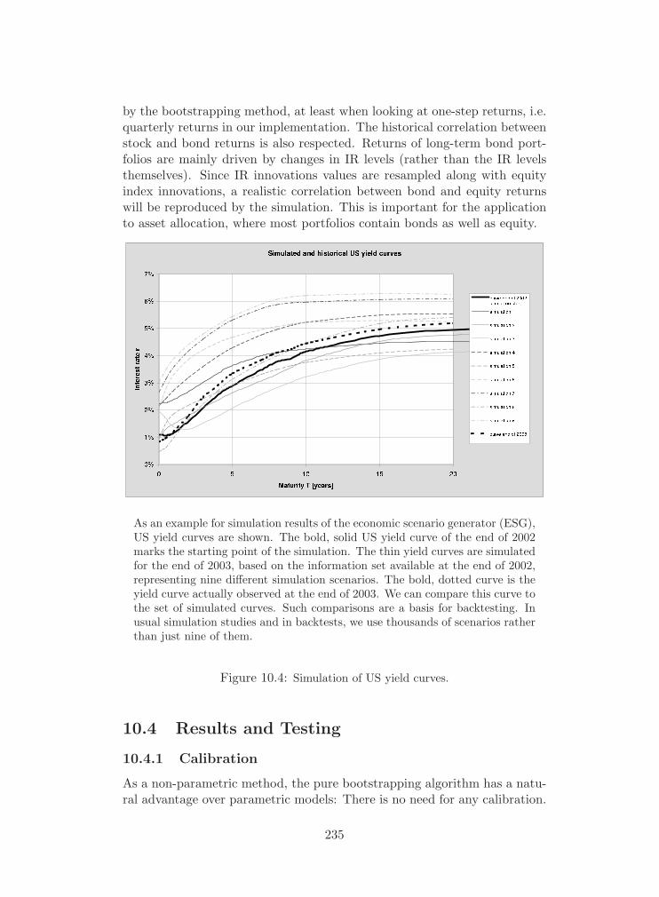
by the bootstrapping method, at least when looking at one-step returns, i.e.quarterly returns in our implementation. The historical correlation betweenstock and bond returns is also respected. Returns of long-term bond port-folios are mainly driven by changes in IR levels (rather than the IR levelsthemselves). Since IR innovations values are resampled along with equityindex innovations, a realistic correlation between bond and equity returnswill be reproduced by the simulation. This is important for the applicationto asset allocation, where most portfolios contain bonds as well as equity.
As an example for simulation results of the economic scenario generator (ESG),US yield curves are shown. The bold, solid US yield curve of the end of 2002marks the starting point of the simulation. The thin yield curves are simulatedfor the end of 2003, based on the information set available at the end of 2002,representing nine different simulation scenarios. The bold, dotted curve is theyield curve actually observed at the end of 2003. We can compare this curve tothe set of simulated curves. Such comparisons are a basis for backtesting. Inusual simulation studies and in backtests, we use thousands of scenarios ratherthan just nine of them.
Figure 10.4: Simulation of US yield curves.
10.4 Results and Testing
10.4.1 Calibration
As a non-parametric method, the pure bootstrapping algorithm has a natu-ral advantage over parametric models: There is no need for any calibration.
235

Historical behaviors are reproduced in the simulated future. If past behav-iors provide a reliable guidance for future behaviors (which is not always anaccurate assumption), the simulated results will automatically be in line.
On a subordinated level, our refined bootstrapping method has someparametric elements such as some mapping formulas, GARCH and smallcorrections of market expectations, mainly the weak mean-reversion effectsof some variables. The models of these refinements rely on a few parametersthat were calibrated by some special studies during the development phase.Some calibrations are done as a preparatory step at the beginning of eachnew scenario generation, based on the same historical data that are also usedby the bootstrapping method. This is the case for the GARCH calibrationsas presented in the Appendix 10.6.
At the end of our development process, some experienced finance special-ists looked at many graphs with first simulation results. Given the complex-ity of setting up a comprehensive set of calibration and testing procedures,the value of judgments by human experts on real-life results should not beunderestimated.
Although a calibration procedure may lead to an in-sample quality mea-sure of a model, it does not provide an independent, reliable quality test.At the end, an out-of-sample test is necessary to finally assess a scenariogenerator and its results.
10.4.2 Example of Results: Yield Curve Simulation
An economic scenario generator produces a wealth of results: many completescenarios for many economic variables, simulated over many time steps. InFigure 10.4, we show a tiny part of these results for the example of simulatedUS yield curves. The historical curve for the end of 2002 marks the startingpoint of the simulations. The nine simulated curves are for the end of 2003,based on four quarterly simulation steps. Each curve belongs to a complete,consistent scenario for all economic variables, including interest rates withtimes to maturity up to 30 years, yield curves for all currencies and manyother variables. Although the simulation period is just one year, we see avariety of yield curve forms on different levels. Simulation 3 has an inversionfor maturities up to two years, simulation 6 has a more humped form.
The true US yield curve at the end of 2003 is also plotted in Figure 10.4 asa bold, dotted curve. It lies slightly above the curve of 2002. The simulatedcurves show a wider range of deviations. This indicates a considerable IRrisk at start of 2003; the actual move in 2003 was rather small in comparison.The overall IR level increased, which is in line with the majority of simulatedcurves. The very low short rate at the end of 2003 is below most of thesimulated values, indicating a particular low-rate policy of the US FederalReserve.
236

10.4.3 Out-of-Sample Backtesting
Our quality testing method is backtesting, see e.g. Christoffersen [2003].Comparisons between historical variable values and their prior scenario fore-casts, as in Figure 10.4, are a basis for backtesting. In Chapter 8 of Christof-fersen [2003], backtests are proposed for three different types of forecasts:(1) point forecasts for the value of a variable, (2) probability range forecasts(e.g. the value at risk [VaR] which is the projected quantile at a certainprobability, often 1%) and (3) forecasts of the complete probability distri-bution. Such distribution forecasts are the most comprehensive type as theyimply range forecasts and point forecasts (using the mean or median of thedistribution, for example).
Scenarios produced by a scenario generator are no forecasts in the usualsense. In typical studies, we produce many thousands of scenarios. Each ofthese scenarios has its own forecast value for a certain variable at a certainfuture time. All the scenario values together define an empirical distributionfor the variable. Hence we have distribution forecasts rather than just pointor range forecasts.
Our task is comprehensive out-of-sample backtesting of distribution fore-casts. Even the limited task of testing specialized models such as an interestrate model is difficult, as discussed in Section 1.5.2 of James and Webber[2000]. Here we propose a methodology based on the Probability IntegralTransform (PIT). Diebold et al. [1998, 1999] have introduced the PIT (alsoknown as Levy or Rosenblatt Transform) as a method for testing distri-bution forecasts in finance. The whole test is described in detail in Blum[2004]. This is a summary of the steps:
1. We define an in-sample period for building the bootstrapping methodwith its innovation vectors and parameter calibrations (e.g. for theGARCH model). The out-of-sample period starts at the end of thein-sample period. Starting at each regular time point out-of-sample,we run a large number of simulation scenarios and observe the scenarioforecasts14 for each of the many variables of the model.
2. The scenario forecasts of a variable x at time ti, sorted in ascendingorder, constitute an empirical distribution forecast. In the asymp-totic limit of very many scenarios, this distribution converges to themarginal cumulative probability distribution Φi(x) = P(xi < x|Ii−m)that we want to test, conditional to the information Ii−m available upto the time ti−m of the simulation start. In the case of a one-step fore-cast, m = 1. The empirical distribution Φi(x) slightly deviates from
14Our main test is for one-step forecasts where the simulation is for one time step (aquarter in our case). Multi-step forecasts can be tested using the same methodology, butthe number of available independent observations with non-overlapping forecast intervalswill be distinctly smaller, given the same out-of-sample period.
237
this. The discrepancy Φi(x) − Φi(x) can be quantified by using a for-mula given by Blum [2004]. Its absolute value is less than 0.019 witha confidence of 95% when choosing 5000 scenarios, for any value of xand any tested variable. This is accurate enough, given the limitationsdue to the rather low number of historical observations.
3. For a set of out-of-sample time points ti, we now have a distributionforecast Φi(x) as well as a historically observed value xi. The cumu-lative distribution Φi(x) is used for the following Probability IntegralTransform (PIT): Zi = Φi(xi). The probabilities Zi, which are con-fined between 0 and 1 by definition, are used in the further course ofthe test. A proposition proved by Diebold et al. [1998] states that theZi are i.i.d. with a uniform distribution U(0, 1) if the conditional dis-tribution forecast Φi(x) coincides with the true process by which thehistorical data have been generated. The proof is extended to the mul-tivariate case in Diebold et al. [1999]. If the series of Zi significantlydeviates from either the U(0, 1) distribution or the i.i.d. property, themodel does not pass the out-of-sample test.
Testing the hypotheses of U(0, 1) and i.i.d. can now be done by using anysuitable method from statistics. We pursue two approaches here:
1. An approach which we call non-parametric is suggested by Dieboldet al. [1998, 1999]. It consists of considering histograms in order todetect deviations from the U(0, 1) property, and correlograms of theZi’s and their low integer powers to detect deviations from the in-dependence property. We complement these graphical evaluations bythe usual χ2 test for uniformity, and by Kendall-Stuart bounds for thesignificance of the autocorrelations.
2. Chen and Fan [2004] suggest another approach, which we call para-metric. It relies on the assumption that the Zi’s form a Markov chainwith stationary distribution G∗(.) and copula C∗(., .) for the depen-dence structure of (Zi, Zi−1). One can then select some model for G∗(.)which contains U(0, 1) as a special case, and some model for C∗(., .)which contains the independence copula as a special case. The jointnull hypothesis of independence and uniformity can then be tested bystandard likelihood ratio or Wald procedures. We specifically use theFarlie-Gumbel-Morgenstern copula as a model for dependence struc-ture and the β-distribution as a model for the marginal distribution.In a semi-parametric variant of this procedure, no model for G∗(.)is chosen, but the empirical distribution of the Zi’s is plugged in in-stead. This allows to test for the isolated hypothesis of independence,irrespective of the marginal distribution.
238
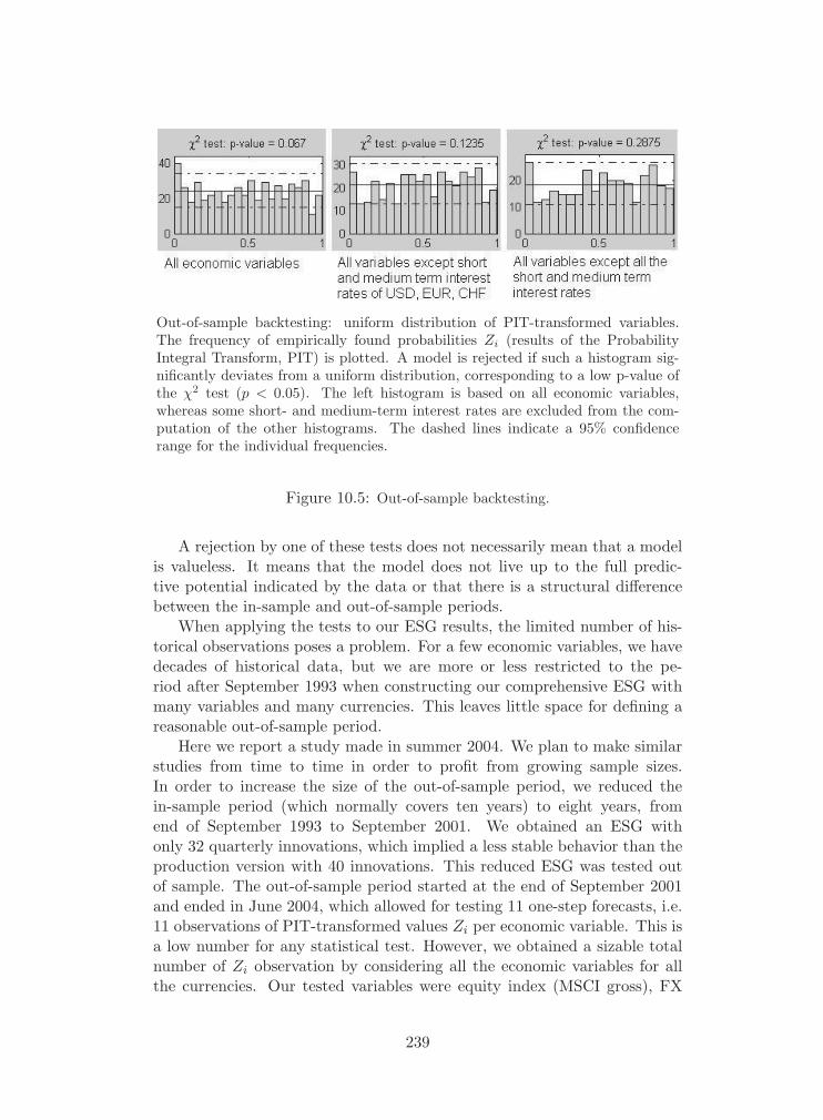
Out-of-sample backtesting: uniform distribution of PIT-transformed variables.The frequency of empirically found probabilities Zi (results of the ProbabilityIntegral Transform, PIT) is plotted. A model is rejected if such a histogram sig-nificantly deviates from a uniform distribution, corresponding to a low p-value ofthe χ2 test (p < 0.05). The left histogram is based on all economic variables,whereas some short- and medium-term interest rates are excluded from the com-putation of the other histograms. The dashed lines indicate a 95% confidencerange for the individual frequencies.
Figure 10.5: Out-of-sample backtesting.
A rejection by one of these tests does not necessarily mean that a modelis valueless. It means that the model does not live up to the full predic-tive potential indicated by the data or that there is a structural differencebetween the in-sample and out-of-sample periods.
When applying the tests to our ESG results, the limited number of his-torical observations poses a problem. For a few economic variables, we havedecades of historical data, but we are more or less restricted to the pe-riod after September 1993 when constructing our comprehensive ESG withmany variables and many currencies. This leaves little space for defining areasonable out-of-sample period.
Here we report a study made in summer 2004. We plan to make similarstudies from time to time in order to profit from growing sample sizes.In order to increase the size of the out-of-sample period, we reduced thein-sample period (which normally covers ten years) to eight years, fromend of September 1993 to September 2001. We obtained an ESG withonly 32 quarterly innovations, which implied a less stable behavior than theproduction version with 40 innovations. This reduced ESG was tested outof sample. The out-of-sample period started at the end of September 2001and ended in June 2004, which allowed for testing 11 one-step forecasts, i.e.11 observations of PIT-transformed values Zi per economic variable. This isa low number for any statistical test. However, we obtained a sizable totalnumber of Zi observation by considering all the economic variables for allthe currencies. Our tested variables were equity index (MSCI gross), FX
239

rate15 against the USD, CPI and GDP. We added four interest rates to thisset of variables, namely the extremes on our maturity scale, the three-monthand the 30-year rates, and two intermediate rates with times to maturityof two years and ten years. Thus we obtained eight variables for each ofthe six currency zones (USD, EUR, JPY, GBP, CHF, AUD). We linked thesmall Zi series of all variables together to obtain a set of 528 (= 11 · 8 · 6)observations of Zi.
The χ2 test of the 528 Zi observations and the underlying histogram isshown on the left-hand side of Figure 10.5. The p-value of 0.0607 exceedsthe confidence limit of 0.05. The ESG forecasts are not rejected, but thelow p-value does not instill wholehearted confidence. An autocorrelationanalysis reveals a marginally significant first-lag autocorrelation between theZi. The semi-parametric evaluation has a high p-value and does not rejectthe ESG forecasts. The likelihood ratio test of the parametric evaluation,which is the most powerful test, significantly rejects the null hypothesis ofi.i.d. U(0, 1) with a p-value of only 0.00021, which is far below a confidencelimit of 0.05.
We have to accept the fact that the ESG forecasting method was re-jecteded by our most powerful test. Fortunately, the testing methods alsoinformes us on what exactly is rejected, and why. A closer look at the inves-tigated out-of-sample period shows that our out-of-sample period is charac-terized by a fundamental difference from the in-sample period. It covers aneconomic situation after a marked decline of equity markets. The worseningeconomic situation caused low demand, low inflation and low interest rates.Most importantly, the US Federal Reserve chose a distinct policy whichkept short-term interest rates low and the US yield curve artificially steep.This policy is specific to the years 2001–2004 and distinctly different fromthe policies of the in-sample period and the 1980s. It led to low values oflow and medium term interest rates, much lower than the market forecastsbased on forward interest rates indicated16. The example of Figure 10.4 canbe seen as an illustration of the unexpectedly low short-term interest ratescaused by this policy. In the first histogram of Figure 10.5, the low ratesmaterialize in the significantly high frequency of Zi values in the leftmostbar.
Our hypothesis is that the unusual low-interest policy is the reason forthe rejection of the forecasts. We test this hypothesis by excluding the three-month, two-year and ten-year interest rates, so the 30-year rate is the onlyinterest rate in the test. In an analysis called study B, we do this only forthe currencies USD (directly affected by the US Feral Reserve policy) and
15For the currency USD, choosing the FX rate against itself makes no sense. Instead,we added a US hedge-fund index to the US-based variables to be tested.
16Some traders made a successful bet on the persistence of this anomaly and madeprofitable carry trades. They financed long-term deposits by rolling short-term debtsforward.
240
EUR and CHF, where the central banks followed similar, if less pronouncedpolicies. Thus the currencies JPY, GBP and AUD still have a full coverageof interest rates. Study B has a sample of 429 Zi observations. In study C,we exclude short and medium term interest rates for all currencies and arriveat a sample of 330 observations. In both studies, B and C, the ESG forecastsare no longer rejected by any test. The χ2 tests have p-values of 0.1235 (B)and 0.2875 (C), both on the good side of the confidence limit of 0.05, seethe middle and right histograms of Figure 10.5. The strongest test, theparametric evaluation, confirms this with p-values of 0.2313 (B) and 0.6017(C). We conclude that the ESG forecasts are rejected only in the case of lowand medium term interest rates of USD, EUR and CHF. Thus we report aqualified success of our ESG forecasts.
Is there a way to improve the method in order to give optimal forecastsfor all variables? This is only possible if factors such as the policy of the USFederal Reserve or, more generally, economic cycles can be predicted. Nei-ther the bootstrapping method nor any of its algorithmic modifications areable to do this, to our knowledge. Long data samples covering many decadesand many economic cycles would help, but we are restricted to shorter sam-ples for most of the modeled economic variables. Shifts in policies, economiccycles and market structures make future developments less predictable. Inour bootstrapping method, a way to accommodate this would be to aug-ment the resampled innovations by a slowly growing factor. Technically,this can be done the same way as the tail correction of Section 10.2.10,using Equation (10.9) with an increased cycle uncertainty multiplier.
A new test planned for 2008 will produce more significant results becausethe size of its out-of-sample period will more than double in comparison tothat of the summer 2004 study. The plan is to repeat the test regularlyusing a newly developed, automated testing environment.
Although the tests based on PIT are powerful, they cannot test all possi-ble aspects of model quality. Several competing models or simulation meth-ods might pass a PIT-based test at the same time, but one model might stillbe better than another17. Some properties stay untested in our PIT-basedmethod, most notably the dependence between returns of different variablesin the simulated scenarios. We have added a study comparing correlationsof simulated returns to those of actual returns, with good results. This isexpected for a bootstrapping method which preserves dependencies in theinnovations by design.
17Example: Some variables might follow a complex nonlinear process that is capturedby model A, whereas model B sees the same behavior as random noise. While none ofthe models is rejected in a PIT-based test, the nonlinear model A is better as it predictsnarrower distributions.
241
10.5 Conclusion
Refined bootstrapping is our method to generate realistic scenarios of thefuture behavior of the global economy as represented by a set of key vari-ables. We have presented many details that need to be observed in order toarrive at a realistic behavior of many different economic variables such asinterest rates, foreign exchange rates, equity indices, inflation and GDP forseveral currency zones. A careful treatment of these modeling details, whichinclude some subordinated parametric elements, is vital for the success ofthe bootstrapping method.
The following advantages of the bootstrapping method have been found:
� Wide coverage of economic variables, modularity and flexibility whenextending the set of covered economic variables
� Automatic preservation of distributions and simultaneous dependen-cies between the innovations of different economic variables
� Exact reproduction of initial conditions at simulation start (no fittingof a model needed for that)
� Feasibility of long-term simulations (over decades), due to mean-reversionelements in expectations of variables
� Natural transition from the short-term behavior at start to the long-term behavior
� Easy ways to introduce modifications based on special studies or expertopinion (e.g. assuming expected equity returns lower than the meanof the historical sample)
� Good coverage of extreme risks, relying on the tail correction of Sec-tion 10.2.10 and large numbers of simulations
� No large calibration problems because the method is essentially non-parametric
Out-of-sample tests have confirmed the validity of the approach. A cer-tain problem arises from the behavior of short and medium term interestrates of some currencies, reflecting an unusual low-interest policy of centralbanks during the out-of-sample period. We have discussed this behavior andpossible solutions.
The final goal of our project has always been the application of themethod in practice. We have implemented the refined bootstrapping methodin our economic scenario generator (ESG). The results are regularly appliedto Asset-Liability Management (ALM) studies that are part of the strategicdecision making of the analyzed companies. We plan to include corporate
242
yield spreads and possibly other economic quantities to the set of boot-strapped variables in order to add new asset classes such as corporate bondsto ESG-based asset allocation studies.
10.6 Appendix: Robust Calibration of a GARCHProcess
In Equation (10.8), a GARCH(1,1) process is defined. In our application, weneed an especially robust calibration procedure. Following Zumbach [2000],we do not directly calibrate the three parameters α0, α1 and β1. We ratherreformulate the equation for the conditional variance as follows:
σ21 = σ2 + μcorr [μema σ2
i−1 + (1 − μema r2i−1) − σ2] , (10.41)
μcorr = α1 + β1 , μema =β1
μcorr, σ2 =
α0
1 − μcorr
The parameters μcorr and μema have values between 0 and (less than) 1.While μcorr describes the decay of the memory in conditional volatility, μema
determines the depth of averaging in the formation of the volatility memory.The unconditional variance σ2 is no longer regarded as a model param-
eter to be optimized through maximum likelihood. Instead, we directlytake the empirical variance of the raw innovations as the moment estimatorfor σ2. Thus we make sure that the unconditional variance of the processequals the empirical variance even if the GARCH process is misspecified orfinite-sample problems lead to difficult behavior.
The two parameters μcorr and μema remain to be calibrated. The result-ing GARCH(1,1) embeds two other processes18: ARCH(1) if μema = 0 anda Gaussian random walk (Brownian motion, white noise) if μcorr = 0. Inthe latter case, the value of μema becomes irrelevant.
The GARCH equation is evaluated iteratively at each time series pointwith index i. Therefore all μ parameters correspond to an exponential decaywith time constant τ :
μcorr = e−1/τcorr , μema = e−1/τema (10.42)
τcorr = − 1log μcorr
, τema = − 1log μema
(10.43)
where the τ values are in units of the time step of the time series.If the maximum-likelihood procedure leads to a μ very close to 1, the
time constants τ may reach extremely high values. Reason demands that18Zumbach [2000] transforms μcorr and μema to other fitting variables by further map-
ping. We do not follow that approach as it pushes ARCH(1) and white noise (which areperfectly acceptable solutions) far away to the asymptotic limits of the parameter space.
243

we do not choose a time constant exceeding the sample size. This is whyour robust method sets an upper limit for τ :
τmax = f n
where n is size of the sample used for fitting and f a constant factor; weusually take f = 0.5. If we use a 10-year sample, for example, we do not ac-cept decay models with time constants longer than five years. At the limit,there are only two five-year volatility clusters within the 10-year sample,at maximum. Two observations are not a large amount in statistics. Thisfact may lead to an intuitive understanding of why we are not willing to ac-cept even longer clusters with even lower significance in our robust GARCHfitting procedure. Our condition is
0 ≤ τcorr ≤ τmax , 0 ≤ τema ≤ τmax (10.44)
μcorr ≤ e−1/τmax , μema ≤ e−1/τmax (10.45)
where the conditions for μ are derived from (10.42). (10.43). The un-constrained solution of most practical fitting cases anyway obeys (10.44),(10.45). However, in some misspecified or small-sample cases, the maxi-mum likelihood may lie outside those conditions, and we prefer the robustsolutions ensured by Equation (10.44), 10.45. The stationarity condition,μcorr = α1 + β1 < 1, is always fulfilled by the slightly stronger μcorr con-dition of Equation (10.44), (10.45). Our solutions not only observe thestationarity limit condition but also keep a safe distance from that limit.
The logarithm of the likelihood function19 is
l(μcorr, μema) = − 12 n
n+m∑i=m+1
[ln 2π + ln σ2
i +r2i
σ2i
](10.46)
with a total number of n + m observations in the sample. We reserve aconsiderable number m of initial observations for the build-up of σ2
i . Atstart (i = 1), we use the initial value
σ20 = σ2
which has an initial error that exponentially declines over the GARCH it-erations, Equation (10.41), from i = 1 to m. The larger m, the smaller isthe remaining error of σ2
i . However, the remaining sample of size n alsobecomes smaller, given a limited total size n + m. This is a trade-off. In
19This formulation assumes that εi is generated by a Gaussian random process, whichis an acceptable assumption for our low-frequency data and the limited role of GARCHwithin the whole bootstrapping algorithm. Assuming another distribution of εi leads toa different log-likelihood function.
244

our low-frequency case with quarterly data, this trade-off is almost desper-ate. A 10-year sample has 40 quarterly observations – a modest number.We need these 40 observations for the likelihood function in order to pro-duce meaningful results. Reserving 20 observations for build-up and usingthe remaining, meager 20 observations for GARCH fitting does not seemto be a reasonable approach. For some economic variables, we have pastdata older than ten years that we can use for the build-up. For some othertime series, this is not available. As a numerical trick, we can recycle thescarce available data to build up an initial σ2
i through a zig-zag method.We create a synthetic past. The real data are r2n+1 . . . r3n, so m = 2n;the synthetic past consists of r1 . . . rn with ri = r2n+i and rn+1 . . . r2n withri = r4n+1−i. This is justified as the innovations ri are already detrendedand their temporal coherence, which is important for GARCH, is respected,though partially in reverse order. We claim that the thus obtained σ2
2n valueis a better approximation of the true value than a simple initialization σ2
2n =σ2. Of course, this claim should be substantiated through a theoretical orstatistical study.
Now we have to determine the maximum of the log-likelihood of Equa-tion (10.46) by varying the parameters μcorr and μema under the constraintsof Equations (10.44), (10.45). This cannot be done analytically. The solu-tion of this non-linear optimization problem can be done with the help ofany appropriate method. All numerical methods lead to a local optimumdepending on the initial guess of parameter values. In order to obtain theglobal optimum, it is important to run the optimization from different initialparameters and to take the best among the obtained solutions. For someGARCH(1,1) processes with large values of both μcorr and μema, the whitenoise solution (μcorr = 0) appears as a local optimum that is dominated bythe true, global optimum. Therefore one should always start optimizationsfrom at least two initial points: (1) white noise and (2) close-to-maximumvalues of μcorr and μema.
245

11
Interest Rate Hedges
Under the definition of interest rate hedges we classify those financial in-struments that react to interest rate increases with an increase in marketvalue. Within an investment portfolio such negative duration instrumentsrepresent a hedge against the losses that the bond investments would incurin case interest rates increase.
The document to describe the interest rate hedges is Debora Iannuzzi,Modelling of interest rate hedges in Converium’s internal ALM model, (Ian-nuzzi [2007]). The model for interest rate hedges is primarily determined bypricing formulas in conjunction with economic scenario generation (ESG),the latter amply documented in Muller et al. [2004]. The document on theinterest rate hedges (Iannuzzi [2007]) aims to specify the type of the repli-cating assets and their pricing methods. This documentation of a model forinterest rate hedges follows Iannuzzi [2007].
SCOR Switzerland’s portfolio currently has two classes of negative du-ration instruments in the three main currencies, USD, EUR and GBP:
� Swaptions with 6-month or 1-year maturity
� Structured notes with 5- or 10-year maturity: the Digital Notes, issuedby the Bayerische Hypo- und Vereinsbank AG (HVB)
The economic scenario generator (ESG) generates scenarios of yieldcurves with a quarterly time granularity. The scenarios are imported inGiulio1 and therein linearly interpolated to daily steps. In correspondenceof each of these daily scenarios Giulio calculates the market value of thehedges, as described in the following sections.
1Gulio is SCOR Switzerland’s asset and liability model written in Igloo. The stochasticsimulations based on the market risk model are largely performed in Igloo which is atechnology applied in the simulation of multivariate probability distributions. MonteCarlo simulations of assets and liabilities are written in Igloo. For an overview of ITsystems we refer to the documentation of IT Systems (Part VIII).
246

11.1 Swaptions
The price of the swaptions is calculated via traditional methods of optionpricing (see Chapter 18 of Neftci [2004]).
Each swaption is assumed to hedge a portfolio of bonds (there are usu-ally more swaptions for the same portfolio, with different durations). Thecorresponding bond portfolio is defined simply as the portfolio of bonds thathave the same currency as the swaption (independent of the duration). Weassume that the ratio R between the swaption notional and the bond port-folio is given. This ratio can be considered as an intrinsic property of theswaption itself.
The swaptions are assumed to follow a rollover strategy. At expiry,each swaption is sold at market value and a new swaption is bought withthe same duration and currency as the previous. The maturity of the newswaption is assumed to be always one year and the strike rate 75bps out-of-the-money. To calculate the notional needed for the swaption the modelcalculates the market value of the corresponding bond portfolio at the timeof the transaction and multiplies it by the aforementioned ratio R.
This rollover strategy mimics the behavior of the asset manager ensuringthat the swaption notional follows the market value of the bond portfoliothat is intended to be hedged. We do not need to redefine the duration ofthe new underlying swaps because we assume that the asset manager followsa strict allocation target, including duration and currency splits. The bondportfolio, as well as the whole asset portfolio, is reallocated once a year (inthe middle of the year) in such a way that the asset allocation, durationand currency split at the beginning and at the end of the year are the same.The reallocation takes into account all cash in- and outflows, including thetrade of the swaptions. For the details regarding bond and equity modelingsee Chapters 12 and 13 in this documentation.
11.2 Structured Notes
The structured notes require an initial investment, the nominal value of thenote, which is guaranteed to be returned at expiry (after five or ten yearsfrom the issue date, depending on the contract). Within the life-span of theproduct, the bank will pay a certain coupon for each day when the referenceinterest rate is above a trigger rate, which was determined at inception ofthe product. The coupon is defined as a function of the reference rate, whichis fixed once a year. In formulae, if N is the notional, T the trigger rate, Lthe reference interest rate (in our case the Libor in a given currency, variableon a daily basis) and Y the reference rate (equal to the Libor, but fixed once
247
a year), then the coupon C (annualized) is defined as2
C =
{0, if L < T
1.99NY if L ≥ T(11.1)
It is clear that, when interest rates increase, the market value of thenotes will increase as well. Therefore these products will be typically chosenby investors who want to protect their bond portfolio against losses derivingfrom extreme increases in interest rates.
The calculation of the market value of the notes as a function of theinterest rate curve is not straightforward. For ease of implementation, wehave chosen a valuation method discussed with the issuing bank, HVB. Theresulting valuation formula can be seen as a polynomial approximation ofwhat the correct valuation formula would be.
The method is based on the so called delta buckets. In short, the methodprovides, for each note, yield shift and maturity, the impact of a shift of25bps on the market value (excluding accrued interest) expressed as a per-centage of the current market value of the note. The delta buckets areprovided to SCOR Switzerland by HVB on a regular basis. For consistencyreasons, HVB delivers also the volatility of SCOR Switzerland’s swaptionsas of the date of the analysis of the notes. Such volatility is the one cur-rently used in the option pricing formula. No volatility modeling is currentlyimplemented.
The delta buckets method allows us to estimate the market value of thenotes at the end of the year excluding the accrued interests. The couponpayments and the accrued interests are then easily calculated as a functionof the reference Libor rates simulated by the ESG model according to theformula expressed by Equation (11.1).
Given that the five- or ten-year maturity notes had inception at theend of 2006, no rolling strategy is needed yet. The notes interact with therest of the portfolio just due to the cash flow they produce via the couponpayments. Also this cash flow is assumed to happen in the middle of the yearand reinvested within the rolling strategy of the rest of the asset portfolio.
11.3 Final Goal
The final goal of these hedging instruments is to lower the risk contributionof the fixed income portfolio to the shareholder equity worst case scenarios.This, of course, can only be monitored when the full ALM model is updated,whereas on a more frequent basis we can monitor stand-alone risk figures ofthe fixed income portfolio with and without interest rate hedges.
2The proportionality factor in Equation (11.1) is chosen consistently with the treatyinformation contained in the contracts between the company and its banking partners.
248

11.4 Sensitivity
The sensitivity analysis of the interest rate hedges is done using the samemethodology described so far: option pricing for the swaptions and bucketdelta method for the notes. The only difference is that the analysis is donein an Excel file instead of Giulio. The same file is also used to crosscheckthe results of Giulio.
11.5 Valuation Formulae
11.5.1 Swaptions
Inputs:
� Expiry of the option Eop
� End of swap Esw
� Strike rate r
� Fixed leg Lfix (which is 1 for EUR, 0.5 for GBP and USD)
� Notional (million) N
� Yield yi at time i (interpolated, if necessary)
� Volatility σ
Valuation Formula: The market value at time t (given the assumptionsregarding the rollover strategy, for us t is always smaller than or equal toEop) is
Mt = NA [P · Φ(D1) − r · Φ(D2)]
where Φ(·) denotes the cumulative of the standard normal distribution, andwe used
A = Lfix
∑i
(1 + yi)−(i−t)
with the time intervals i determined according to the time leg Lfix. P isthe par yield
P =1A
[(1 + yEsw)−(Esw−t) − 1
]while D1 and D2 are defined as
D1 =ln(
Pr
)+ 1
2σ2(Eop − t)σ√
Eop − t
D2 = D1 − σ√
Eop − t
249

11.5.2 Notes
Inputs:
� Notional (million): N
� Accrued interest up to the valuation time t (actual - for the springexercise – or estimated using the reference yield curve and Equation(11.1) – for the autumn exercise): M0
� Bucket delta matrix with entries Aij (for each note and each projectiondate different) where i is the delta shift with steps of 25bps (from –300to +300bps) and j is the maturity (j = 0m, 3m, 6m, 9m, 1y, 2y, 3y,4y, 5y, 7y, 8y, 9y, 10y, 11y)
� Reference yield curve (provided by the bank) (fj)j=0m,··· ,11y where jis the maturity
Valuation formula: From the matrix Aij we extract, by linear inter-polation, the matrix Bkj where k is the delta shift with steps of 1bp.Then the market value M is defined as a function of a generic yield curveG = (gj)j=0m,··· ,11y:
M(G) = N
gj−fj∑k=0
11y∑j=0m
(Bkj + M0)
250

12
Bond Portfolio Management
12.1 Introduction: Bonds, Equities, Cash
Simulating stochastic time series of bond and equity portfolios implies match-ing the cash flows between assets and liabilities (Muller [2006c]). Cash flowmanagement is an essential ingredient to the risk model. While cash flowsfrom or to the insurance liabilities are determined by the liability com-ponents themselves, the cash flows from and to the assets are subject toallocation guidelines. Cash flow management acquires an adjustment func-tion when imbalances arise between the various asset classes caused by theinhomogeneous performance of asset classes. In multi period simulationsthe cash flows assigned to an asset component are modeled on the followingassumptions: For each of the simulated time steps information is receivedfrom the modeled asset classes about the market values and return factors.The desired market value share which shall be sustained at the end of asimulation step must be additionally specified for each asset portfolio. Theexchange of cash flows takes place at mid period of each simulated timeinterval in a multi period simulation.
Accounting for equity portfolios has been explicitly modeled (Muller[2006a]). The equity portfolio can be of the most general type, includinghedge funds and real estate investments. The model assumes a continuousreinvestment of dividend payments. For the purpose of the model the initialconfiguration of an equity component is defined by the currency, the ini-tial market and book values, the inclination to realize unrealized currencygains in excess of the realizations due to necessary transactions and similarspecifications. The economic scenario generator (ESG) delivers the foreignexchange (FX) rates, return rates and dividend yields. External cash flowsfrom and to the portfolio are modeled by the cash flow management (Muller[2006c]).
The bond portfolio model mimics a bond portfolio manager (Muller[2007a]). The bonds considered are of the highest possible maturity, govern-
251

ment bonds. Portfolios of bonds are modeled by an algorithm which governsthe roll over of the portfolio and is determined by target values to be keptconstant, either mean time to maturity or duration. For the purpose of astylized bond portfolio in multi period simulations the roll over happensat the midpoint of each simulated time interval. The bond with shortesttime to maturity is then sold and a new bond with much longer maturity isbought. The entire scenario depends on the economic scenario generator forzero coupon yield curves and foreign exchange rates. The policies are set atinitialization stage by defining the turnover intensities in excess of the nec-essary turnover, historical coupon rates, the inclination to realize currencygains, the choice of the target variable (held to maturity or duration), themode of the rollover, e.g. rolling at maturity, the currency and others. Inmulti-period simulations the number of bonds and their maturities held ina stylized portfolio are algorithmically inferred at each simulated time step.External cash flows from or to the portfolio are modeled in the cash flowmanagement (Muller [2006c]).
Corporate bond portfolios are affected by default risks and are consideredunder the credit risk model (Muller [2007b]). The credit risk model conceivesof a corporate bond as of the sum of a credit derivative of initial value zeroand a risk free bond (government bond); which illustrates the link betweencredit risk and market risk (Muller [2007b]).
The models for equity, bonds and cash flows are firmly placed withinthe framework of stochastic economic simulation (Muller et al. [2004]) andare documented in Accounting of an equity portfolio in simulations, Bondportfolio management and accounting in simulations, Managing cash flowsof assets and liabilities by Ulrich A. Muller (Muller [2006a], Muller [2007a],Muller [2006c]), a slightly edited version of which we are going to present inthis and the following two chapters.
12.2 Bond Portfolios in Simulations
In the framework of ALM components written in Igloo1, the SCOR Switzer-land Financial Modeling (FinMod) team uses a bond portfolio componentwhich is able to manage a portfolio of bonds with predefined properties suchas duration over the course of a Monte Carlo simulation, including proper ac-counting. The economic input for simulations, most importantly simulatedyield curves, comes from an economic scenario generator (ESG).
An intelligent scheme of rollover and rebalancing of the bonds is neededto maintain the required properties of the portfolio over time. The goal isto mimic the behavior of fund managers tracking a target such as a meantime to maturity or a bond index, using a simplified scheme of bonds in
1For an overview of this IT system we refer to the SST Systems documentation in PartVIII of this document.
252

a regular sequence of maturities. Even a simple model requires a rathercomplex computation of market values. The accounting variables such asbook value, realized and unrealized gains, coupon income, amortization andimpairment loss require an even larger number of carefully developed cal-culation formulas. The main application will need pro-forma accounting inUS GAAP style, but the results can also be used for other standards.
Our bond portfolio management encompasses a consequent observance ofthe mean-time-to-maturity target, straightforward initialization of all vari-ables, full support of market values and all accounting variables in localcurrency and accounting currency and total transparency of all formulasand algorithms.
Extreme precision of accounting results is not required since the resultsare based on simulated scenarios, and the internal details of the bond port-folio (such as the coupons and maturities of thousands of individual bondsof the portfolio) are treated in an aggregate, simplified form by an efficientmodel. The goal is the simulation of realistic projected balance sheets andincome statements.
12.3 Timing: The Simulation Period
The simulation tool (Igloo2 or any other tools such as ReMetrica) has a basicsimulation period of fixed size Δt. The simplest choice is yearly simulationfrom year end to year end. If this temporal resolution is insufficient, we maychoose a multi-step approach with many small time steps such as quarterlyperiods.
The method allows for unlimited multi-period simulation. We keep thetreatment of individual time steps as simple as possible, so the only wayto achieve higher precision or temporal resolution is to choose smaller timesteps in a multi-step approach. The first simulation period starts at thelast regular time point for which full information on the portfolio and theeconomic variables is available. In each simulation scenario, new periods canbe added by using the final values of the previous period as new startingpoints.
Cash flows from and to the bond portfolio typically happen over a wholeperiod, not just at its beginning or its end. In order to have an efficient cashflow management in an ALM model with dozens of asset-and-liability com-ponents, we assume just one time point of the period at which all the cashflows happen instantaneously. Whenever this appears to be a too coarse sim-plification, we can use the same remedy as already stated above: replacingthe large period by a sequence of shorter ones.
There is one reasonable choice for the time of the cash flow: the middleof the period. This is the average of all cash flow times, assuming that
2See also Part VIII, pp. 408.
253

these are uniformly distributed over the year. Choosing the cash flow timeat mid-period is in line with accounting-based concepts such as average FXrates and average investment levels.
Another advantage of the chosen concept is that we have stable situationsand variable values (including mean time to maturity or duration) at boththe beginning and the end of the simulation period, where the accounting ismade.
For an appropriate bond portfolio treatment, we are forced to model asimplified internal structure explicitly, whereas an equity portfolio can bemodeled in aggregated form. This internal structure leads to internal cashflows (coupons, rollover, reestablishment of the desired portfolio duration)which are assumed to happen at the midpoint of the period. In that respect,the internal cash flows are treated like the external ones.
12.4 The Stylized Bond Portfolio
The bond portfolio is a bunch of bonds denominated and expressed in onelocal currency, managed as an entity with a consistent policy (e.g. mean-time-to-maturity or duration target) and with continuous reinvestment ofcoupon payments.
The portfolio composition may be complicated in reality, with thousandsof bonds. Modeling every bond of a real-life portfolio and simulating therollover to hundreds of new bonds is regarded as inefficient. On the otherhand, treating all bonds in a portfolio as one unstructured object probablyleads to inaccurate results, given a simulated behavior of the full yield curve.This motivates us to go for an intermediate approach. We model few stylizedbonds in a regular sequence of maturities. In the further course of the modelexplanation, we usually talk about n stylized bonds, but we stay aware ofthe fact that each of the n bonds acts as a proxy for another sub-portfoliowhich may again consist of many individual securities.
Real-life bond managers usually have a mandate with guidelines. Beforebonds expire, they are typically sold, and new bonds are bought from theproceedings of the sale and the paid coupons. Through such a rolloverprocedure, the managers can achieve the desired goal of keeping either themean time to maturity or the duration constant. In our approach, there isexactly one such rollover per simulation period which stands as a proxy forthe whole set of real-life rollover operations during the period.
The bond portfolio does not exchange any funds with the outside world,except for a one-time cash flow from or to it at the middle of the simulationperiod. This one-time cash flow may have different external causes: claimpayments, rebalancing between asset classes, investing new income.
The bond portfolio also has some internal cash flows due to reinvestedcoupons and reshuffling of the portfolio. These are not part of that external
254

cash flow and are regarded as an internal affair of the portfolio, invisible toother components. True coupon payments may be annual or semiannual orquarterly, depending on the type of the bond. Regardless of that frequency,the issuing dates, maturity dates and payment dates of the many real-lifebonds are irregularly scattered over the whole period. Thus it would bearbitrary if we artificially defined some fixed semiannual payment dates,with so-called par yields based on semiannual payments. Instead, we alwaysoperate with annualized coupon rates (which can be calculated to correspondto par yields or any other coupon payment scheme as closely as possible),and we use only one yield curve, the zero-coupon spot yield curve. Par yieldcurves play no role, but users may translate the model results back to suchconcepts if so desired. Moreover, we assume exactly one payment time forcoupons in the middle of the simulation period (which serves as a proxy andan average time of many such payments scattered over the year). Everyalternative convention would add a lot of complexity to the cash flow timingwith no clear gain in overall modeling accuracy.
A bond portfolio modeled as described may also stand for a bond index,if that is a total-return index. Bond indices are usually set up with similarrules as our model portfolio, keeping the mean time to maturity or durationroughly constant over time. Thus the algorithm described here can also beused to explore the future behavior of a bond index in simulations.
The ESG provides economic scenarios for the zero-coupon yield curveswhich determine the behavior of each bond of the portfolio. The marketvalue of each bond is given by the present value (PV) of the future cashflows.
The bonds are assumed to have the highest possible rating (governmentbonds). Future cash flows are assumed to be certain. Impairments of bondinvestments are therefore excluded. The modeling of bonds with credit riskand default risk (corporate bonds) is discussed under the credit risk model(Chapter 18).
12.5 Input Variables
A modeled bond portfolio encompasses many real-life bonds, all in the samecurrency, and maps them into a series of few stylized bonds. At initializationof a bond portfolio component, we know a few characteristic properties:
� The legal entity to which the bond portfolio is assigned
� The currency of the bond portfolio (= local currency)
� The accounting mode, held to maturity (HTM) or available for sale(AFS), where the trading mode may be approximately treated likeAFS
255

� The initial market value of the whole portfolio, MVinit, in local cur-rency
� The corresponding initial book value BVinit in local currency
� The initial level of the currency translation adjustment, CTAaccinit (the
part of unrealized gains that is due to currency shifts prior to thesimulation start, which is the sum of the two items Group UR CcyGain and Group UR Ccy Loss in Mellon’s reporting tool)
� The choice of the target variable to be kept constant, either mean timeto maturity (MTM) or duration (D)
� The target value T (for MTM) or D of the target variable, e.g. adesired duration of D = 4 years, assuming that the portfolio is ontarget with respect to that variable already at simulation start
� The maturity Tr at which the rollover of each stylized bond has tobe executed (= minimum accepted time to maturity), must be 0 (=rolling at maturity, a typical choice for held-to-maturity securities) ora positive integer multiple of the basic time interval Δt, e.g. one year;a reasonable choice is clearly less than T or less than D, respectively
� Historical coupon rate assumed for the stylized bonds at initialization,either individual for each bond or simply an average historical couponrate Chist, assuming that all stylized bonds initially have that one
� The average, relative coupon level c of newly purchased bonds, as afraction of the current interest rate level, where c = 0 indicates a policybased on zero-coupon bonds and c = 1 indicates par bonds (assumingthat the coupons of newly bought bonds equal the simultaneouslyobserved zero-coupon yield, on average)
� The turnover intensity u of the bond portfolio in excess of the necessaryturnover needed to reinvest coupons and re-establish allocation targets,with 0 ≤ u ≤ 1 (further discussed in Section 12.11)
� The FX turnover intensity uFX of the bond portfolio, the inclinationto realize unrealized currency gains in excess of realizations due tonecessary transactions, with 0 ≤ uFX ≤ 1 (further discussed in Sec-tion 12.12)
These variables refer to particular bond portfolios. In addition to these,there are some economic variables which affect all bond portfolios. An eco-nomic scenario generator (ESG) provides the necessary information, for thestart as well as the end of a simulation step:
256

� The initial zero-coupon yield curve of the local currency, with interestrates rinit(T ), where arbitrary maturities 0 < T ≤ 30 years are sup-ported (through interpolation between the standard maturities of theESG);
� The final zero-coupon yield curve of the local currency, with interestrates rfinal(T ), analogous to rinit(T ) but for the end time of the period;
� The initial foreign exchange (FX) rate faccinit (= value of one unit of
local currency expressed in the accounting currency);
� The final FX rate faccfinal (analogous to facc
init but for the end time of theperiod).
All variables with superscript acc are expressed in the accounting (orconsolidation) currency. If that index is missing, the quantity is expressedin the local currency of the bond portfolio.
Some initial variable values directly follow from the input variables above,so we can compute them right away. The following formulas apply to anytype of asset, not just bond portfolios. The initial level of unrealized gains(or losses, if < 0) in local currency is
Uinit = MVinit − BVinit
The initial market value in accounting currency is
MVaccinit = facc
init MVinit
The book value in accounting currency is listed in the Mellon reporting toolunder the header Group Book. We do not extract that quantity from there,however, because it can be computed with the help of the initial CTA:
BVaccinit = BVinit
(faccinit −
CTAaccinit
MVinit
)
This can be interpreted as the book value translated to the accounting cur-rency based on an old FX rate f ′acc
init rather than the current one:
f ′accinit = facc
init −CTAacc
init
MVinit=
BVaccinit
BVinit(12.1)
This is the FX rate that was used when the bond portfolio was bought (ora weighted mean of such rates for a complex portfolio that was graduallybuilt up in the past). The level of unrealized gains in accounting currencyis
U ′accinit = MVacc
init − BVaccinit = Uacc
init + CTAaccinit (12.2)
The last form shows that the unrealized gains consist of two components:one due to changes in the asset market, Uacc
init, and one due to changes in the
257
FX rate, CTAaccinit. In the Mellon reporting tool we find U ′acc as the sum of
the two items Group UR Gain and Group UR Loss. In our application wedo not take it from there but rather compute it through Equation (12.2).When simulating US GAAP balance sheets we want to know the the twocomponents of the unrealized gain separately. We compute Uacc
init as
Uaccinit = U ′acc
init − CTAaccinit
12.6 The Bond Portfolio: Overview of theAlgorithm
The stylized model portfolio, which stands for a more complicated real-lifeportfolio, has a fixed set of n bonds with regular times to maturities Ti atthe beginning of a simulation period:
Ti = Tr + (i − 0.5) Δt = (m + i − 0.5) Δt , 1 ≤ i ≤ n (12.3)
withm =
Tr
Δt
The shortest time to maturity is thus Tr + 0.5Δt. At the midpoint of theperiod, this time interval shrinks to Tr, which is the rollover maturity. Nowthe rollover happens: The bond is sold and a new bond with a much longertime to maturity, Tr + nΔt, is bought. At that time we shift the indices ofall the bonds. The second-shortest bond takes the role of the shortest oneand takes the index i = 1, followed by an analogous index shift for all otherbonds. The new bond obtains the index n. At the same time there maybe some additional and modified transactions due to reinvested coupons,external cash flows and the re-establishing of the target MTM or duration.At the end of the period, there are still n bonds which then have the sametimes to maturity as those of Equation (12.3).
The scheme is set up in a way that the mean time to maturity, averagedover a whole period, is indeed close to T . At period start and end, it isexactly so. In the first half of the period, it naturally shrinks by half theperiod size, but this is compensated by the rollover, after which the meantime to maturity exceeds T by half the period size. In the second half, itmoves back to the target value T .
12.7 Initial Bond Portfolio Set-Up
At the beginning of the first simulation period, the stylized bond portfoliohas to be defined in line with the input parameters. At the beginning ofa subsequent simulation period in a multi-period simulation, the state of
258

the bond portfolio is already known from the previous period. Thus thefollowing initialization of the portfolio only applies to the first period.
The choice of n depends on Tr and the target of MTM or duration. Ifthe mean time to maturity (T ) is the target, a reasonable choice is
n = ceiling[2
T − Tr
Δt
](12.4)
where ceiling [.] denotes the lowest integer number equal to or exceeding theargument. In order to have at least one bond, n = 1, we need the condition
Tr < T
The case n = 1 is unusual as there is only one bond that is replaced byanother one at mid-period. This property limits the flexibility of reachingany given target MTM value, so we normally exclude the case n = 1.
If the target is duration instead of MTM, we use a rule of thumb for asuitable choice of n which slightly deviates from Equation (12.4). Only thecase of MTM is pulled through. A duration target can be treated analo-gously.
We denote the coupon rate of each bond by Ci. The coupon rate of allinitial bonds of the initial period is assumed to be Chist. Starting at the firstrollover, other coupon rates come into play.
For all n bonds, we can now compute the initial market value per unitof principal, based on Ti, the coupon Ci and the initial zero-coupon yieldcurve:
MV∗init,i = Ci
m+i∑j=1
{1 + r[(j − 0.5) Δt]}−(j−0.5) Δt1 year (12.5)
+{1 + r[(m + i − 0.5) Δt]}−(m+i−0.5) Δt1 year
This is the usual formula for the present value of discounted cash flows. Themarket values MVi of the bonds also depend on the size of the principals orredemption values Pi:
MVinit,i = Pi MV∗init,i (12.6)
We do not know MVinit,i or Pi at the beginning, but we allocate theinvestment in a way to conform to the given input parameters through asimple linear allocation scheme:
Pi = a Ti + b (12.7)
The parameters a and b are determined by two conditions, namely the totalinitial market value MVinit,
MVinit =n∑
i=1
MVinit,i =n∑
i=1
Pi MV∗init,i (12.8)
259

and the target MTM (= T ) which is exactly observed at initialization, lead-ing to
MVinit T =n∑
i=1
MVinit,i Ti =n∑
i=1
Pi MV∗init,i Ti (12.9)
These equations, combined with Equation (12.7), lead to two linear equa-tions for a and b with the solution
a =
MVinit
∑ni=1 MV∗init,i Ti − T
∑ni=1 MV∗init,i
(∑n
i=1 MV∗init,i Ti)2 − (∑n
i=1 MV∗init,i)(∑n
i=1 MV∗init,i T 2i )
and
b =MVinit − a
∑ni=1 MV∗init,i Ti∑n
i=1 MV∗init,i
For n > 1, there is always a unique solution {a, b} which can be reinserted inEquation (12.7) and then (12.6). Now we have all the relevant information onthe initial bonds and their market values. At the beginning of a subsequentsimulation step, the initialization procedure is not repeated because theallocation then is simply given as the final allocation of the previous step.
12.8 The Bond Portfolio at the Midpoint of thePeriod
The midpoint of the period is the time of all internal and external cash flowsin our model. Before these cash flows, the portfolio keeps the same allocationwith the same principals as at the beginning, given by Equation (12.7). Themarket value however changes in the first half of the period, for two reasons.The bonds are closer to maturity, and the yield curve is different. The ESGdoes not provide yield curves at the midpoints of periods. Lacking thatinformation, the best approach is interpolation, which just means averagingin our case:
rmid(T ) =rinit(T ) + rfinal(T )
2Of course there might be alternative averaging schemes, e.g. geometric av-eraging of yield factors or an interpolation based on initial forward interestrates.
At the midpoint, each of the n stylized bonds pays a coupon:
Cpaid,i = Ci Pi
All coupons together have a value of
Cpaid =n∑
i=1
Cpaid,i (12.10)
260

Immediately after the coupon payments and before the rollover and theexternal cash flow, we obtain the following market value for each bond, perunit of principal:
MV∗beforeC,i = Ci
m+i−1∑j=1
[1 + rmid(j Δt)]−j Δt1 year (12.11)
+{1 + rmid[(m + i − 1) Δt]}−(m+i−1) Δt1 year
This is like Equation (12.5), except that maturity periods are reduced by halfa period length (Δt/2), one more coupon payment has already happened,and the updated interest rates rmid are used.
The bond with index 1 is now reaching the rollover point and is sold forits market value,
Proceedings = P1 MV∗beforeC,1
which can be computed by using Equation (12.11).Neither the coupon payments nor the sale of a bond leads to a change in
the total portfolio value including the coupons paid and the sale proceedings,which is
MVbeforeC =n∑
i=2
Pi MV∗beforeC,i + Proceedings + Cpaid (12.12)
where the first term denotes the value of the remaining bonds and the lasttwo terms the available free cash.
After the sale of the bond with index 1, the portfolio still has n − 1bonds. We rename those bonds by diminishing the index of each bond by 1.The bond closest to maturity now has the index 1 instead of 2. The indexn becomes free and will be used for a new bond. All the following equationsare based on the new indices.
A new bond with index n and time to maturity Tr + n is going to bebought now in order to complete the rollover. This time to maturity is inline with all current times to maturity of the new portfolio:
Tmid,i = Tr + i Δt = (m + i) Δt , 1 ≤ i ≤ n
Notice the effect of the index shift and the fact that maturity periods arereduced by half a period length, Δt/2, as compared to Equation (12.3) atperiod start. The times to maturity at the end of the period can also becomputed:
T ′i = Tr + (i − 0.5) Δt = (m + i − 0.5) Δt , 1 ≤ i ≤ n (12.13)
where the maturity periods are again reduced by half a period length, Δt/2.This equation is the same as Equation (12.3), except for the fact that theindex i now denotes different bonds.
261

The coupon rate Cn of the new bond depends on the market and theinvestment policy and may deviate from Chist. We use
Cn = c rmid[(m + n) Δt]
where the input variable c stands for the coupon policy as explained inSection 12.5.
The market value of each bond, per unit of principal, is still given byEquation (12.11). We reformulate that equation by using the new, shiftedindices i:
MV∗afterC,i = (12.14)
Ci
m+i∑j=1
[1 + rmid(j Δt)]−j Δt1 year + {1 + rmid[(m + i) Δt]}−(m+i) Δt
1 year
This formula is also valid for the new bond with index i = n. The corre-sponding market values per unit of principal at period end can be computedsimilarly:
MV∗final,i =
Ci
m+i∑j=1
{1 + rfinal[(j − 0.5) Δt]}−(j−0.5) Δt1 year
+{1 + rfinal[(m + i − 0.5) Δt]}−(m+i−0.5) Δt1 year
Here we are using the interest rates rfinal at period end, and times to maturitythat are reduced by half a period size.
A simple rollover rule would be to use the total amount of free cash,Cpaid+Proceedings, for buying the new bond. We need a more sophisticatedrule, for two reasons. First, the bond portfolio receives some cash from theoutside world or has to deliver cash. Second, we have to observe a targetfor the MTM or the duration. We can reach the target through a fullrebalancing exercise which may lead to some shifts of the bond allocation inaddition to the purchase of the new bond.
In reality, the bond managers are maintaining a duration target in con-tinuous time, within a certain tolerance range, so the MTM or the durationis on target at every moment, including the end of the period. In our modelwe have all cash flows virtually concentrated at mid-period, but the MTMor duration only matters at the end of the period, where results are reportedto users. We solve this problem by choosing an allocation now that will ex-actly reach the target at period end, which is possible as we already knowthe economic variable values at period end. We are forced to consider thefurther development of the portfolio already now.
Immediately after the external cash flow, the total market value of theportfolio, including cash, is
MVafterC = MVbeforeC + CF (12.15)
262
where MVbeforeC comes from Equation (12.12) and the cash flow CF is apiece of external information produced in the course of the simulation, as tobe further discussed in Section 12.9.
The total market value MVafterC is now allocated by using a similarprocedure as in the initial allocation. Since we do not know MVafterC yet,we can only determine relative allocation pi of principals now. The pi val-ues will eventually be scaled by a yet unknown constant to arrive at thetrue principals. This allocation is again defined as following a simple linearscheme as in Equation (12.7):
pi = a′ T ′i + b′ (12.16)
where T ′i is defined by Equation (12.13). The pi values are constant overthe whole second half of the simulation period, including its end, where themarket values MV∗final,i per unit principal are given by Equation (12.7). Weare free to define the pi values as scaled in a way to reach a final marketvalue of 1:
1 =n∑
i=1
pi MV∗final,i (12.17)
This is one condition to find the a′ and b′ values, analogous to Equation(12.8), but now per unit market value at the period end. The second condi-tion states that the target MTM (= T ) will exactly be observed at periodend, leading to
T =n∑
i=1
pi MV∗final,i T ′i
analogous to Equation (12.9). Now we have two linear equations for a′ andb′ with the solution
a′ =∑ni=1 MV∗final,i T ′i − T
∑ni=1 MV∗final,i
(∑n
i=1 MV∗final,i T ′i ) (∑n
i=1 MV∗final,i T ′i ) − (∑n
i=1 MV∗final,i)(∑n
i=1 MV∗final,i T ′2i )
and
b′ =1 − a′
∑ni=1 MV∗final,i T ′i∑n
i=1 MV∗final,i
Since n > 1, there is always a unique solution {a′, b′} which can be re-inserted in Equation (12.16). The value of the portfolio with an allocationof principals pi is
∑ni=1 piMV∗afterC,i after the cash flow and grows to 1 over
the second half of the simulation period, see Equation (12.17), so the growthfactor expressed in the local currency is
g =1∑n
i=1 pi MV∗afterC,i
(12.18)
This growth factor applies to the whole amount of the investment, regardlessif it originates from an old investment or from cash newly injected andinvested at mid-period.
263

12.9 Cash Flow from or to the Portfolio
At the midpoint of the simulation period, a cash flow comes into play. Thesize of this cash flow is essentially determined by the outside world. Cashenters in case of general premium growth and profitable underwriting, cashmay be demanded from the component if claim payments exceed premiumincome.
However, the bond portfolio component also exerts a limited influenceon the determination of the cash flows between components. The reasonis rebalancing. Typical investors try to keep the allocation to different as-set classes constant, which may require some shifts of cash between assetportfolios from time to time. These rebalancing cash flows can only be com-puted by an external cash flow management component (the treasurer ofthe model) if some information on market values is known there. The bondportfolio component has to provide some information before it gets back thedesired information on the cash flow.
In Igloo, such circular information loops are not allowed. This is whywe have to technically divide the bond portfolio component into two com-ponents:
1. The initial bond portfolio component is configured by the initial valuesof Section 12.5 (in the first simulation period) or the final values ofa previous period and passes some information on its market valuedevelopment to the cash flow manager.
2. The final bond portfolio component receives some basic informationfrom its initial sister component and the cash flow information fromthe cash flow manager. Then it computes all results of the simulationperiod.
Rebalancing may encompass assets denominated in different currencies,but it is defined in terms of the accounting currency. The cash flow man-agement is also done in accounting currency. In order to support cash flowcalculations, we need to know the foreign exchange rate facc
mid at cash flowtime. In accounting, such an average rate is sometimes provided. In theframework of our period-based simulations, we have no such informationand choose the following obvious assumption:
faccmid =
faccinit + facc
final
2(12.19)
The aim is to have a well balanced portfolio at the end of the simulationperiod, at the time and in the currency of the accounting. A perfect balanceat the period midpoint is not necessary as this midpoint is just an auxiliarytime point with no accounting results to be shown to the users.
The cash flow manager thus needs the following information to make aninformed decision on asset rebalancing:
264

� the market value faccmidMVbeforeC at mid-period, just before the cash
flow, in accounting currency, where MVbeforeC is available from Equa-tion (12.12);
� the growth factor gacc by which the portfolio and the injected cashflow will appreciate between the middle and the end of the period,expressed in accounting currency.
The growth factor gacc is
gacc = gfaccfinal
faccmid
and thus has a dependency on the FX market. The local growth factor gresults from Equation (12.18). If cash is withdrawn from the bond portfolio,gacc refers to the size of the reduction caused by the withdrawal.
The cash flow manager (see Chapter 14, pp. 287) then determines thesize of the cash flow CFacc to the component. In order to obtain the valuein local currency, the final bond portfolio component has to do a division bythe FX rate,
CF =CFacc
faccmid
This can be inserted in Equation (12.15). The cash flows CFacc and CF canbe positive or negative. In the latter case, the cash drain may be as highas to make the whole market value MVafterC negative. That extreme event,which can only happen in case of bankruptcy, will in fact never be seen if weuse a smart cash flow manager component with realistic insolvency handlingor at least a cash overdraft component for negative market values.
12.10 The Bond Portfolio at the End of the Period
After inserting the cash flow in Equation (12.15), we obtain the market valueMVafterC, which allows the final bond portfolio component to compute allthe relevant results at the end of the simulation period. The final marketvalue in local currency is
MVfinal = g MVafterC (12.20)
The principals Pi in the second half of the simulation period can becomputed as
Pi = MVfinal pi (12.21)
using the results of Equation (12.16).The final market value in accounting currency is
MVaccfinal = MVfinal facc
final (12.22)
265

In a multi-period simulation, the end state of the portfolio is identicalto the initial state of the next period. A second simulation period will startfrom here instead of initializing the portfolio from scratch.
At this point of the description, we know all necessary things about thedevelopment of market values, but we do not yet fully support accountingviews.
12.11 Accounting Results in Local Currency
The book value of the bond portfolio and other accounting variables are af-fected by the cash injection or withdrawal at mid-period and by the turnoverpolicy of the asset manager. The accounting is first dealt with in the localcurrency. Then we move to the accounting currency, where the CTA comesinto play.
Each bond has a book value which is defined similar to the market valueas the present value of the future cash flows, except for using a fixed, frozeninterest rate instead of the current yield curve for discounting. At the startof the simulation, we have the relation
BVi =
Ci Pi
m+i∑j=1
(1 + yi)−(j−0.5) Δt
1 year + Pi (1 + yi)−(m+i−0.5) Δt
1 year (12.23)
which is similar to Equation (12.5) combined with Equation (12.6). Theinterest rates of the yield curve are now replaced by the fixed interest rate yi,the so-called yield to maturity of the bond. This quantity stays constant overthe lifetime of a bond, once the bond has been purchased. It is annualizedonly if the simulation time period Δt has the size of 1 year. Otherwise itrefers to the period Δt rather than 1 year.
The sum in Equation (12.23) is now a regular geometric series as yi isidentical for all coupon payment dates. Using the sum formula for geometricseries, we obtain
BVi = Pi (1 + yi)0.5
[Ci
yi+
1 − Ciyi
(1 + yi)m+i
](12.24)
In case of a zero yield, yi = 0, this equation numerically diverges. We canreplace 0 by a very small number then.
We have a problem as we often have to compute the yield yi of each styl-ized bond from the book value rather than the other way around. Equation(12.24) cannot be inverted analytically in a closed form for that purpose.We need an iterative procedure such as IRR() of Excel. In Igloo simulations,where we have to compute thousands of yi values, we prefer not using an
266
iterative algorithm. Instead, we replace Equation (12.24) by an approxi-mation that is analytically invertible. We expand the expression up to thesecond order of yi, but we write y′i instead of yi to emphasize the fact thatthe expansion is just an approximation:
BVi = Pi1 + (m + i) Ci + [1 + (Mi + m + i) Ci] y′i
1 + (m + i + 0.5) y′i + [Mi + 0.5 (m + i) + 0.25] y′i2 (12.25)
withMi = 1.3
(m + i) (m + i − 1)2
The original second-order expansion does not have the factor 1.3 in thisequation. We prefer using the factor 1.3 because it approximates the effect ofthe omitted higher-order terms and leads to smaller average approximationerrors.
When using a correct BVi and then solving Equation (12.25) for y′i, thisy′i will be a good approximation of the true yi.
The expansion of Equation (12.25) is set up as a rational function ofy′i rather than a simple polynomial. An equivalent polynomial expansionexists, but some terms are negative there and may lead to a negative bookvalue if y′i has an extreme value. We avoid that numerical problem by usingEquation (12.25) where all terms in the numerator and the denominator arepositive, so the book value is always positive, even for extremely large y′i.
Equation (12.25) can be solved for y′i through a quadratic equation:
y′i = (12.26)
Bi +√
B2i − 4 [Mi + 0.5 (m + i) + 0.25] BVi
Pi[BVi
Pi− 1 − (m + i) Ci]
2 [Mi + 0.5 (m + i) + 0.25] BViPi
withBi = 1 + (Mi + m + i) Ci − (m + i + 0.5)
BVi
Pi
The resulting yield y′i is a reasonable approximation of the true yield for asufficiently wide range of different maturities, coupon rates and yields. Thequality of the approximation is shown in Table 12.11 for different choices ofthose parameters. Some unusually high values of coupons (12%) and yields(15%) are also considered there because these values challenge the qualityof the approximation more than moderate values.
Whatever the maturities, coupons, and yields from Equation (12.26),Equation (12.25) exactly reproduces the original book value BVi, leading toa consistent behavior of the algorithm with no unwanted jumps in BVi dueto approximation errors.
267
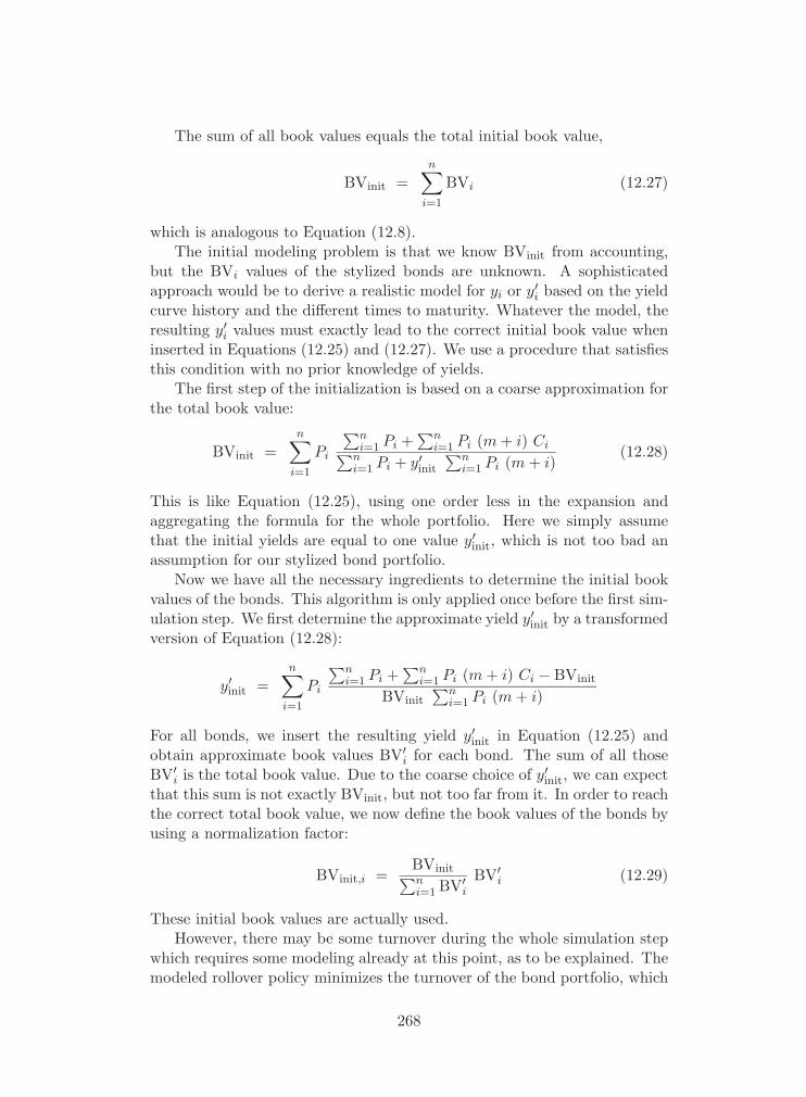
The sum of all book values equals the total initial book value,
BVinit =n∑
i=1
BVi (12.27)
which is analogous to Equation (12.8).The initial modeling problem is that we know BVinit from accounting,
but the BVi values of the stylized bonds are unknown. A sophisticatedapproach would be to derive a realistic model for yi or y′i based on the yieldcurve history and the different times to maturity. Whatever the model, theresulting y′i values must exactly lead to the correct initial book value wheninserted in Equations (12.25) and (12.27). We use a procedure that satisfiesthis condition with no prior knowledge of yields.
The first step of the initialization is based on a coarse approximation forthe total book value:
BVinit =n∑
i=1
Pi
∑ni=1 Pi +
∑ni=1 Pi (m + i) Ci∑n
i=1 Pi + y′init
∑ni=1 Pi (m + i)
(12.28)
This is like Equation (12.25), using one order less in the expansion andaggregating the formula for the whole portfolio. Here we simply assumethat the initial yields are equal to one value y′init, which is not too bad anassumption for our stylized bond portfolio.
Now we have all the necessary ingredients to determine the initial bookvalues of the bonds. This algorithm is only applied once before the first sim-ulation step. We first determine the approximate yield y′init by a transformedversion of Equation (12.28):
y′init =n∑
i=1
Pi
∑ni=1 Pi +
∑ni=1 Pi (m + i) Ci − BVinit
BVinit∑n
i=1 Pi (m + i)
For all bonds, we insert the resulting yield y′init in Equation (12.25) andobtain approximate book values BV′i for each bond. The sum of all thoseBV′i is the total book value. Due to the coarse choice of y′init, we can expectthat this sum is not exactly BVinit, but not too far from it. In order to reachthe correct total book value, we now define the book values of the bonds byusing a normalization factor:
BVinit,i =BVinit∑ni=1 BV′i
BV′i (12.29)
These initial book values are actually used.However, there may be some turnover during the whole simulation step
which requires some modeling already at this point, as to be explained. Themodeled rollover policy minimizes the turnover of the bond portfolio, which
268
more or less corresponds to the behavior of real asset managers. The rolloverhappens at mid-period and affects book values only then, not at the startof the period, so the initial book values BVinit,i are not affected.
Some asset managers may however generate some additional turnoverfor whatever reason, for example index tracking or corporate bond picking.We only refer to that additional turnover when using the word turnover inthe following derivations. This turnover may happen at any time during thesimulation period, but a practical implementation requires that we formallyconcentrate all the modeled turnover activities at very few time points. Wemight model them to happen at mid-period only, like the cash flows, butsuch a model would not be able to include an extreme case which we wantto cover, namely the case of continuous realization of all unrealized gains.That limit case of very high turnover can be included if we allow for turnoverat the period end. We also introduce another moment when turnover canhappen, namely the period start, because the investment size may stronglydiffer between the two halves of the period and we want to model turnoverin both halves.
The turnover in the first half period is modeled as an immediate correc-tion of the initial book value:
BVinitAT,i = MViniti +√
1 − u (BVinit,i − MVinit,i) (12.30)
where the parameter u is the turnover intensity, with 0 ≤ u ≤ 1. If u = 0,there is no turnover, if u = 1, the turnover is so strong that the book valuemoves to the market value. The index initAT means initial after turnover.The book value BVinit,i originates from Equation (12.29) (at start of thefirst simulation step) or is the final book value of the previous simulationstep. The initial market value MViniti can be taken from Equation (12.6).We assume the same u value for all the bonds in our simple turnover model.We always assume that the turnover does not affect the properties of theinvestment because the newly purchased securities have – in our model –the same properties as the old ones. Thus the turnover only leads to shiftsin accounting results, not market values. The turnover causes the followingrealized gain in the first half of the period:
Ginit,i = BVinitATi − BVinit,i
For all bonds together, we obtain
Ginit =n∑
i=1
Ginit,i
The book value BVinitAT,i is now inserted in Equation (12.26) to obtainan individual yield to maturity y′i for each bond. The resulting y′i valuesreplace the coarse approximation y′init in the further course of accounting
269
calculations. The yield y′i of a bond keeps its constant value until maturityis reached (or other securities with the same maturity and another yield areadditionally purchased and then mixed with the initial bond investment).
Maturity (years) 2 2.5 10 10.5
True yieldCoupon rate to maturity
2% 5% 4.98% 4.92% 4.94% 4.93%15% 14.76% 14.45% 15.58% 15.69%
12% 5% 5.00% 5.02% 5.09% 5.01%15% 14.95% 14.52% 15.07% 14.61%
Equation used 12.37 12.26 12.37 12.26
Yields to maturity resulting from approximation formulas applied to exactbook values. A comparison to the true yields shows the approximation qualityin different cases. Unlike the exact formula based on discounted cash flows,the approximations (Equations [12.26] and [12.37]), are analytically invertible(Equations [12.25] and [12.35]), so exact book values are reproduced wheninserting approximate yields to maturity.
Table 12.1: Approximation for yields to maturity of bonds.
After computing the book values and y′i, we also want to know the bookvalues at the end of the period and at the mid-point of the period, wherethe book values serve as intermediary results for computing some furtherresults. In the first half of the period, before coupon payments, rollover andcash flow, the book value is only affected by the progress of time, that is byamortization. At this point, we have the following book values, analogousto Equation (12.11):
BV∗beforeC,i = Ci
m+i∑j=1
[1 + yi]−(j−1) Δt
1 year + {1 + yi}−(m+i−1) Δt1 year (12.31)
where the same yi as at period start applies. For consistency reasons, wetake an approximation analogous to Equation (12.25):
BVbeforeC,i = Pi1 + (m + i) Ci + [1 + (Mi + m + i) Ci] y′i
1 + (m + i) y′i + Mi y′i2 (12.32)
where the same approximate yield y′i as at period start is taken. Equa-tion (12.32) looks slightly different from Equation (12.25) because the firstcoupon of the cash flow projection starts immediately now instead of half a
270

period later. The change in book value is the amortization of the portfolioin the first half of the period:
Amortinit,i = BVbeforeC,i − BVinitAT,i (12.33)
and, for all bonds together,
Amortinit =n∑
i=1
Amortinit,i
The amortization can be positive or negative, depending on the relative sizesof the coupon rates Ci and the yields y′i.
At mid-period, coupons are paid and the oldest bond is sold, as explainedin Section 12.8. The book value of that oldest bond with index n does notmatter as the proceedings of the sale correspond to the market value. Afterthe sale but before the injection or withdrawal of cash, the indices of thebonds are shifted, so the index i = n becomes free for a new bond to bepurchased. The external cash flow also leads to allocation changes as alreadyexplained in Section 12.8. All these steps affect the book values.
For some or all bonds, an additional amount of an already existing bondtype has to be purchased. The problem is that the new amount of a bondwith index i < n may have another yield than the old portion as the yieldcurve may have moved in the meantime. We have already limited the modelcomplexity by assuming that the newly purchased portion has the samematurity and coupon as the existing portion. Now we add the assumptionthat the new bond with index i, which consists of two portions with differentyields, can be treated as a new homogeneous block with one yield, which isa sort of mixed yield of the old and the new portion.
After all transactions and the index shift, the following equation for bookvalues can be formulated, analogous to Equations (12.11) and (12.31):
BV∗mid,i = Ci
m+i∑j=1
[1 + yi]−j Δt
1 year + {1 + yi}−(m+i) Δt1 year (12.34)
For consistency reasons, we again replace Equation (12.34) by an approxi-mation analogous to Equations (12.25) and (12.32):
BVi = Pi1 + (m + i) Ci + Mi Ci y′i
1 + (m + i) y′i + Mi y′i2 (12.35)
where the same approximate yield y′i as for the first half of the period (afterthe treatment of the turnover) is taken, except for the index shift, of course.Equation (12.35) looks slightly different from Equations (12.25) and (12.32)because the first coupon of the cash flow projection starts after one periodinstead of half a period or immediately.
271

After the external cash flow and the re-balancing of the portfolio, theprincipals Pi have changed. We denote the principal before the cash flowby PbeforeC,i; the value results from Equation (12.7) (at simulation start) orEquation (12.21) as computed in the previous period (if we are not in thefirst simulation period). The principal after the cash flow is called Pnew,i
and results from Equation (12.21) as computed in the current period. BothPbeforeC,i and Pnew,i use the new, shifted indices. Now we can calculate thebook values after the cash flow:
BVafterC,i =
{Pnew,i
PbeforeC,iBVbeforeC,i, if Pnew,i < PbeforeC,i
BVbeforeC,i + (Pnew,i − PbeforeC,i) MV∗afterC,i, otherwise
where BVbeforeC,i results from Equation (12.35) by inserting PbeforeC,i andMV∗afterC,i from Equation (12.14). The change in Pi also leads to a newcontribution to the realized gains:
Gmid,i =
{(1 − Pnew,i
PbeforeC,i) (MVbeforeC,i − BVbeforeC,i), if Pnew,i < PbeforeC,i
0, otherwise
For all bonds together, we obtain
Gmid =n∑
i=1
Gmid,i (12.36)
The new book value BVafterC,i is needed to compute the new, mixedyield y′i of both the old portion and the newly purchased portion together.This is done by using the inverted form of Equation (12.35):
y′i =Bi +
√B2
i − 4 MiBViPi
[BViPi
− 1 − (m + i) Ci]
2 MiBViPi
(12.37)
where the auxiliary quantity
Bi = Mi Ci − (m + i)BVi
Pi
is used and the new book and principal values are inserted, BVi = BVafterC,i
and Pi = Pnew,i. Equation (12.37) corresponds to Equation (12.26) whichwas derived for the period start rather than the midpoint.
We use Equation (12.37) for all bonds after the cash flow, including thenewly purchased bond with index n. The only special feature of the newbond is that PbeforeC,n = 0 is inserted in Equation (12.35). This leads to aninitial book value equal to the initial market value of the new bond.
272
Now we can compute the final book values BVfinalBT,i by inserting thenew yields y′i in Equation (12.25). The index finalBT means final before tak-ing the final turnover into account. We can now compute the amortizationin the second half of the period:
Amortfinal,i = BVfinalBT,i − BVafterC,i
which is analogous to Equation (12.33). For all bonds together, we obtain
Amortfinal =n∑
i=1
Amortfinal,i
The resulting BVfinalBT,i values are now corrected by additional turnovermodeled to happen at period end, which stands as a proxy for turnover inthe second half period in general:
BVfinal,i = MVfinal,i +√
1 − u (BVfinalBT,i − MVfinal,i) (12.38)
analogous to Equation (12.30), with the same turnover intensity u. The finalmarket value MVfinal,i can be taken from Equation (12.20). The turnovercauses the following realized gain in the second half of the period:
Gfinal,i = BVfinal,i − BVfinalBT,i
In the case of no additional turnover, which means u = 0, the evaluationof Equation (12.38) is superfluous as BVfinal,i = BVfinalBT,i and Gfinal,i van-ishes. As soon as we have a portfolio with u > 0, we need Equation (12.38)and arrive at a new final book value BVfinal,i, where the bond with index i isa mixture of an old portion and a portion consisting of newly purchased se-curities (due to additional turnover). The two portions have different yields,but we again compute a common, mixed yield y′i for efficiency reasons. Thepreviously computed y′i should then be replaced by a new y′i value whichresults from a repeated application of Equation (12.37) to BVfinal,i.
For all bonds of the portfolio together, we obtain
Gfinal =n∑
i=1
Gfinal,i
and the total, final book value is
BVfinal =n∑
i=1
BVfinal,i
Based on the final book value BVfinal we can compute more accountingvariables. Notice that the accounting of bonds and other fixed income in-vestments may depend on the accounting standard and the category of the
273
investment. The two main categories are available for sale (AFS) and heldto maturity (HTM). The balance sheet is typically based on market valuesof AFS securities and book values of HTM securities. In this document wepresent useful variables to support different accounting standards and dif-ferent categories, but we do not discuss the choice of standard to be used ina particular application.
A first useful variable is the total unrealized gain U at the end of theperiod,
Ufinal = MVfinal − BVfinal
For performance calculations we are sometimes interested in the unrealizedgain ΔU of the period, which is
ΔU = Ufinal − Uinit = MVfinal − BVfinal − (MVinit − BVinit) (12.39)
The income statement focuses on income which consists of three parts,namely the realized gain G, the coupon income Cpaid from Equation (12.10)and the amortization (which is counted as income although there is no im-mediate cash flow):
Income = G + Cpaid + Amort = BVfinal − BVinit − CF (12.40)
The last form states that the income is the change in overall book valueexcluding the external cash flow. The cash flow is excluded because it is notgenerated by the component itself.
The realized gain G of the component is
G = Ginit + Gmid + Gfinal
where the middle term originates from a reduction of the investment size atmid-period (Equation [12.36]) and the other two terms reflect gains due toadditional turnover in the bond portfolio management. Realized gains canof course be negative, in which case we call them realized losses.
The total amortization of bonds in the whole period is computed as thesum of the two period halves:
Amort = Amortinit + Amortfinal (12.41)
The performance of the bond investment can only be measured if boththe realized income and the unrealized gains are considered:
TotalGain = Income + ΔU = MVfinal − MVinit − CF (12.42)
This relation can be derived from Equations (12.39) and (12.40). An invest-ment return of the period can then be calculated by dividing the total gainby the mean market value:
Investment Return =Total Gain
0.5 (MVinit + MVfinal)
274
12.12 Final Accounting Results in AccountingCurrency
The accounting currency is used to do the final accounting and reporting ofthe analyzed company. The currency translation depends on the FX rateused. For the market value we use the final FX rate facc
final, see Equation(12.22), and for income statement variables originating from many timepoints in the course of the period, we use the average rate facc
mid from Equation(12.19).
For the book value and the computation of the currency translation ad-justment (CTA), we need the booked FX rate f ′acc
final which is typically theaverage of rates that prevailed when the assets were bought, similar to f ′acc
init
which we computed in Equation (12.1). A detailed derivation of f ′accfinal would
be based on tracking the FX rates used in all simulated transactions, whichwould be rather complex without adding much value. We prefer a sim-pler but realistic approach. Two effects essentially affect f ′acc
final: additionallypurchased assets (mainly if the cash flow was positive) and deliberate real-izations of the CTA. The Mellon reporting tool indeed shows quite a fewsecurities (often with low investment sizes) with CTA = 0. Initial CTAshave been realized in those cases (or there may be a booking error in theMellon tool). It does not matter whether such a realization is due to realmarket transactions or just a virtual booking operation, as long as it iscorrectly reported. The inclination to perform such CTA realizations is aninput parameter called the FX turnover, uFX, where uFX = 0 means no suchinclination and uFX = 1 means continuous realization of all FX gains andlosses. In practice, uFX often exceeds 0 as reinvested coupons are bookedat new FX rates, thus leading to some natural FX turnover. Our model forf ′accfinal is
f ′accfinal = uFX facc
final + (1 − uFX)MVbeforeC f ′acc
init + max(CF, 0) faccmid
MVbeforeC + max(CF, 0)
where faccmid originates from Equation (12.19) and MVbeforeC from Equation
(12.12). The cash flow of the component, CF, plays an asymmetric role here.As long as it is negative or zero (no new investment), it has no influence onf ′accfinal.
The book value in accounting currency can now be computed:
BVaccfinal = BVfinal f ′acc
final
The total unrealized gain (or loss) is
U ′accfinal = MVacc
final − BVaccfinal = Uacc
final + CTAaccfinal (12.43)
The last form shows the two components of the total unrealized gain thatwe ultimately need in accounting. The unrealized gain excluding currency
275

gains and losses isUacc
final = Ufinal f ′accfinal (12.44)
The Currency Translation Adjustment (CTA) has a final value of
CTAacc = MVfinal (faccfinal − f ′acc
final) (12.45)
This directly shows the impact of the FX rate difference faccfinal−f ′acc
final. Equa-tions (12.44) and (12.45) are consistent with Equation (12.43).
The income to be reported in accounting currency is
Incomeacc = Gacc + Caccpaid + Amortacc = BVacc
final −BVaccinit −CFacc (12.46)
where BVaccinit is the book value at the start of the period. The cash flow
is again subtracted in the last expression because it is external rather thanbeing generated by the component itself. The relation between Income andIncomeacc is not straightforward as Incomeacc additionally contains somerealized currency gains or losses.
The coupon income in accounting currency is
Caccpaid = Cpaid facc
mid
using the FX rate of the time when coupons are reinvested, where Cpaid
originates from Equation (12.10). The amortization of bonds happens overthe whole period, where the booked FX rate is shifting. In lack of a detailedstudy of that rate, we use an average rate for the amortization gain inaccounting currency:
Amortacc = Amortf ′accinit + f ′acc
final
2
where Amort is the result of Equation (12.41). The realized gain Gacc inaccounting currency is not just Gfacc
mid, which is the part due to gains in localcurrency expressed in accounting currency, but it also contains a part dueto realized currency gains. A simple way to compute the total realized gainsGacc follows from Equation (12.46):
Gacc = Incomeacc − Caccpaid − Amortacc
12.13 Income Statement and Simulation PeriodSize
Income related variables as computed above can directly be reported in aprojected income statement if the simulation period is one year. If smallerperiods are used, the contributions of the periods within a year have to beadded in order to produce a yearly income statement. In that case, we mightalso reformulate some equations by using an average FX rate for the wholeyear instead of individual periods.
276

13
Accounting of an EquityPortfolio
13.1 Introduction
In the framework of ALM components written in Igloo1, SCOR Switzerland’sFinancial Modeling team (FinMod) developed an equity portfolio compo-nent which is able to keep track of all relevant accounting variables in thecourse of a Monte Carlo simulation. The equity portfolio can be of the mostgeneral type (including hedge funds and other funds, real estate investmentsetc.). The economic input for simulations comes from an economic scenariogenerator (ESG).
While the evolution of the market value is a straightforward simulationresult, the accounting variables such as book value, realized and unrealizedgains, dividend income and impairment loss require some deeper discussion.The main application will need pro-forma accounting in US GAAP style,but the results can also be used for other standards.
Extreme precision of accounting results is not required since the resultsare based on simulated scenarios, and internal details of the equity portfolio(such as the properties of individual equities in the portfolio) are not known.The goal is the simulation of realistic projected balance sheets and incomestatements.
13.2 Timing: the Simulation Period
Each simulation software (Igloo or any other tool such as ReMetrica) hasits basic simulation period. The simplest choice is yearly simulation fromyear end to year end. If this temporal resolution is insufficient, we maychoose smaller time steps such as quarterly periods. We keep the treatment
1See again Part VIII in this documentation.
277

of individual time steps as simple as possible, so the only way to achievehigher precision or temporal resolution is to choose smaller time steps.
Cash flows from and to the equity portfolio typically happen over thewhole period, not just at its beginning or its end. In order to have anefficient cash flow management in an ALM model with dozens of asset-and-liability components, we assume just one time point of the period at whichall the cash flows happen instantaneously. Whenever this appears to bea too coarse simplification, we can use the same remedy as already statedabove: replacing the large period by a sequence of shorter ones.
There is one reasonable choice for the time of the cash flow: the middleof the period. This is the average of all cash flow times, assuming thatthese are uniformly distributed over the year. Choosing the cash flow timeat mid-period is in line with accounting-based concepts such as average FXrates and average investment levels.
Another advantage of the chosen concept is that we have stable situationsand variable values at both the beginning and the end of the simulationperiod, where the accounting is made.
13.3 The Equity Portfolio
The equity portfolio is a bunch of equities of any kind, expressed in one localcurrency, managed as an entity with a consistent policy and with continuousreinvestment of dividend payments. There is only a one-time cash flow fromor to it at the middle of the simulation period. This one-time cash flow mayhave different external causes: claim payments, rebalancing between assetclasses, investing new income. The cash flow due to the own dividends of theportfolio is not part of that external cash flow and is regarded as an internalaffair of the portfolio, invisible to other components. It has no influenceon any market value, but it affects some accounting variables such as thedividend income as reported in the projected income statement.
We have an economic scenario for the overall behavior of the marketvalue of an equity portfolio. The relevant variable is the total return rate rover the period, assuming that the market value of the portfolio, includingreinvested dividends, is 1 + r times the initial market value. The dividendyield d is also known from the ESG and will be used for accounting purposesonly.
13.4 Input Variables
At initialization of an equity portfolio component, we know the values of afew characteristic properties:
� The legal entity to which the equity portfolio is assigned
278

� The currency of the equity portfolio (= local currency)
� The initial market value of the whole portfolio, MVinit, in local cur-rency
� The corresponding initial book value BVinit in local currency
� The initial level of the currency translation adjustment, CTAaccinit (the
part of unrealized gains that is due to currency shifts prior to thesimulation start, which is the sum of the two items Group UR CcyGain and Group UR Ccy Loss in Mellon’s reporting tool)
� The turnover intensity u of the equity portfolio, with 0 ≤ u ≤ 1 (fur-ther discussed in Section 13.7)
� The FX turnover intensity uFX of the bond portfolio, the inclinationto realize unrealized currency gains in excess of realizations due tonecessary transactions, with 0 ≤ uFX ≤ 1 (further discussed in Sec-tion 13.8)
These variables refer to particular equity portfolios. In addition to these,there are some economic variables which affect the whole equity market. Aneconomic scenario generator (ESG) provides the necessary information, forthe start as well as the end of a simulation step:
� The initial foreign exchange (FX) rate faccinit (= value of one unit of
local currency expressed in the accounting currency)
� The final FX rate faccfinal (analogous to facc
init but for the end time of theperiod)
� The total return rate r of the period (annual only if the period isdefined as one year, otherwise for the period)
� The dividend yield d of the period (annual only if the period is definedas one year, otherwise for the period)
All variables with superscript acc are expressed in the accounting (orconsolidation) currency. If that index is missing, the quantity is expressedin the local currency of the equity index.
Some initial variable values directly follow from the input variables above,so we can compute them right away. The following formulas apply to anytype of asset, not just bond portfolios. The initial level of unrealized gains(or losses, if < 0) in local currency is
Uinit = MVinit − BVinit
The initial market value in accounting currency is
MVaccinit = facc
init MVinit
279

The book value in accounting currency is listed in the Mellon reporting toolunder the header Group Book. We do not extract that quantity from there,however, because it can be computed with the help of the initial CTA:
BVaccinit = BVinit
(faccinit −
CTAaccinit
MVinit
)
This can be interpreted as the book value translated to the accounting cur-rency based on an old FX rate f ′acc
init rather than the current one:
f ′accinit = facc
init −CTAacc
init
MVinit=
BVaccinit
BVinit(13.1)
This is the FX rate that was used when the bond portfolio was bought (ora weighted mean of such rates for a complex portfolio that was graduallybuilt up in the past). The level of unrealized gains in accounting currencyis
U ′accinit = MVacc
init − BVaccinit = Uacc
init + CTAaccinit (13.2)
The last form shows that the unrealized gains consist of two components:one due to changes in the asset market, Uacc
init, and one due to changes in theFX rate, CTAacc
init. In the Mellon reporting tool we find U ′acc as the sum ofthe two items Group UR Gain and Group UR Loss. In our application we donot take it from there but rather compute it through Equation (13.2). Whensimulating US GAAP balance sheets we want to know the two componentsof the unrealized gain separately. We compute Uacc
init as
Uaccinit = U ′acc
init − CTAaccinit
13.5 Cash Flow from or to the Portfolio
The situation is essentially the same as for cash flows from or to bondportfolios (see p. 264). In analogy with the bond portfolio, we divide theequity portfolio component into two components:
1. The initial equity portfolio component is configured by the initial val-ues of Section 13.4 and passes some information on its market valuedevelopment to the cash flow manager.
2. The final equity portfolio component receives some basic informationfrom its initial sister component and the cash flow information fromthe cash flow manager. Then it computes all results of the simulationperiod.
Rebalancing may encompass assets denominated in different currencies,but it is defined in terms of the accounting currency. The cash flow man-agement is also done in accounting currency. In order to support cash flow
280

calculations, we need to know the foreign exchange rate faccmid at cash flow
time. In accounting, such an average rate is sometimes provided. In theframework of our period-based simulations, we have no such informationand choose the following obvious assumption:
faccmid =
faccinit + facc
final
2(13.3)
The aim is to have a well balanced portfolio at the end of the simulationperiod, at the time and in the currency of the accounting. A perfect balanceat the period midpoint is not necessary as this midpoint is just an auxiliarytime point with no accounting results.
The cash flow manager thus needs some information to make an in-formed decision on asset rebalancing. The market value of the portfolio,immediately before the cash flow, is
MVbeforeC = MVinit
√1 + r (13.4)
approximately assuming that the return factor in the first half period equalsthat of the second half. Altogether the cash flow manager thus needs thefollowing information:
� The market value faccmidMVbeforeC at mid-period, just before the cash
flow, in accounting currency
� The growth factor√
1 + rfaccfinal/facc
mid by which the portfolio and injectedcash flow will appreciate between the middle and the end of the period,expressed in accounting currency
If the cash is withdrawn from the equity portfolio, the latter factor alsorefers to the loss caused by the withdrawal.
13.6 Market Value Results
The final equity portfolio component receives a cash amount CFacc from thecash flow manager, corresponding to
CF =CFacc
faccmid
in local currency. Then the component is able to compute the final marketvalue in local currency,
MVfinal = MVinit (1 + r) + CF√
1 + r
and in accounting currency,
MVaccfinal = MVfinal facc
final (13.5)
At this point, we know all necessary things about the development of marketvalues, but we do not yet support accounting views.
281

13.7 Accounting Results in Local Currency
The book value of the equity portfolio and other accounting variables areaffected by several effects. They are listed in the sequence of their treatmenthere:
� Injection or withdrawal of cash at mid-period
� Dividends (which are reinvested)
� Turnover due to internal rebalancing of the equities in the portfolio
� Impairment of some equities depending on the size of losses
The accounting is first dealt with in the local currency. Then we move tothe accounting currency, where the CTA comes into play.
Injected cash is used to buy new equity, where the purchase price equalsthe market value and the book value. Withdrawn cash means the liquidationof some equities, assuming that the book value of the remaining portfoliois diminished by the same proportion as the market value. For a portfoliowithout dividends, internal turnover or impairments, we obtain the followingbook value at the end of the period:
BV′′′final =
{BVinit + CF if CF ≥ 0BVinit + CF BVinit
MVinit√
1+rotherwise
(13.6)
Dividend payments are reinvested and immediately added to the bookvalue. The book value of the equity investments that generated the dividendstays constant. In the absence of internal turnover and impairments, wefurther develop Equation (13.6) and obtain a final book value of
BV′′final = BV′′′final + D
where the reinvested dividend income D is defined as
D = d MVinit +d
2CF (13.7)
Here the dividend is composed of an initial contribution and another termdue to the additional cash flow.
Asset managers hardly keep their equity portfolio totally constant overthe period. If they have a passive index tracking mandate, several trans-actions are necessary to keep the tracking error low. Active managers maychange the composition even more frequently. Whenever some equity is soldduring these turnover processes, unrealized gains or losses are realized, andthe book value of the newly purchased equity equals the market value, thus
282
moving the overall book value closer to the overall market value. In absenceof impairments, the book value at the end of the period is
BV′final = u MVfinal + (1 − u) BV′′final
where the parameter u is the turnover intensity, with 0 ≤ u ≤ 1. Anabsolutely stable portfolio with no internal turnover has u = 0. In the caseof a passive mandate, the turnover is rather low with a roughly estimatedu = 0.2 for a yearly period.
Impairments of individual equity titles are necessary if the market valuemoves below a threshold, a certain fraction of the book value, typically y =80% under US GAAP. In that case, the book value has to be taken backto the market value. The size of this shift is the impairment loss I. Asimple assumption is that an impairment test is made only once, at theend of the period. Another simple assumption states that all equity titlesbehave as fixed proportions of the portfolio. Under these assumptions, afinal impairment test of the whole portfolio leads to the following final bookvalue:
BVsimpleImpairmentfinal =
{BV′final if MVfinal
BV′final
> y
MVfinal otherwise(13.8)
A better approximation models a fraction v of equity titles to be impairedthat can take any values between 0 and 1. If MVfinal/BV′final is around y,the true v is likely to be somewhere in between. A heuristic model can bemade as follows:
v =1
1 +(
MVfinal0.82 y BV′
final
)30
This formula (which might be discussed and refined) leads to the final for-mula of the book value at the end of the period:
BVfinal = v MVfinal + (1 − v) BV′final
The corresponding impairment loss is defined as a positive number:
I = BV′final − BVfinal = v (BV′final − MVfinal) (13.9)
Now we can compute more accounting variables such as the income ofthe component:
Income = BVfinal − BVinit − CF (13.10)
The cash flow is subtracted here because it is external rather than beinggenerated by the component itself. The income is reported in the incomestatement and consists of three parts: realized gains, dividend income andimpairment loss. The latter two quantities are defined by Equations (13.7)and (13.9), so we obtain for the realized gain
G = Income − D + I = BVfinal − BVinit − CF − D + I
283
Another useful variable is the total unrealized gain U at the end of theperiod,
Ufinal = MVfinal − BVfinal
For performance calculations we are sometimes interested in the unrealizedgain ΔU of the period, which is
ΔU = Ufinal − Uinit = MVfinal − BVfinal − (MVinit − BVinit) (13.11)
The performance of the equity investment can only be measured if boththe realized income and the unrealized gains are considered:
TotalGain = Income + ΔU = MVfinal − MVinit − CF
This relation can be derived from Equations (13.11) and (13.10). An invest-ment return of the period can then be calculated by dividing the total gainby the mean market value:
InvestmentReturn =TotalGain
0.5 (MVinit + MVfinal)
13.8 Final Accounting Results in AccountingCurrency
The accounting currency is used to do the final accounting and reportingof the analyzed company. The currency translation depends on the FXrate used. For the market value we use the final FX rate facc
final, see Equation(13.5), and for income statement variables originating from many time pointsin the course of the period, we use the average rate facc
mid from Equation(13.3).
For the book value and the computation of the currency translation ad-justment (CTA), we need the booked FX rate f ′acc
final which is typically theaverage of rates that prevailed when the assets were bought, similar to f ′acc
init
which we computed in Equation (13.1). A detailed derivation of f ′accfinal would
be based on tracking the FX rates used in all simulated transactions, whichwould be rather complex without adding much value. We prefer a sim-pler but realistic approach. Two effects essentially affect f ′acc
final: additionallypurchased assets (mainly if the cash flow was positive) and deliberate real-izations of the CTA. The Mellon reporting tool indeed shows quite a fewsecurities (often with low investment sizes) with CTA = 0. Initial CTAshave been realized in those cases (or there may be a booking error in theMellon tool). It does not matter whether such a realization is due to realmarket transactions or just a virtual booking operation, as long as it iscorrectly reported. The inclination to perform such CTA realizations is aninput parameter called the FX turnover, uFX, where uFX = 0 means no such
284

inclination and uFX = 1 means continuous realization of all FX gains andlosses. In practice, uFX often exceeds 0 as reinvested coupons are bookedat new FX rates, thus leading to some natural FX turnover. Our model forf ′accfinal is
f ′accfinal = uFX facc
final + (1 − uFX)MVbeforeC f ′acc
init + max(CF, 0) faccmid
MVbeforeC + max(CF, 0)
where faccmid originates from Equation (13.3) and MVbeforeC from Equation
(13.4). The cash flow of the component, CF, plays an asymmetric role here.As long as it is negative or zero (no new investment), it has no influence onf ′accfinal.
The book value in accounting currency can now be computed:
BVaccfinal = BVfinal f ′acc
final
The total unrealized gain (or loss) is
U ′accfinal = MVacc
final − BVaccfinal = Uacc
final + CTAaccfinal (13.12)
The last form shows the two components of the total unrealized gain thatwe ultimately need in accounting. The unrealized gain excluding currencygains and losses is
Uaccfinal = Ufinal f ′acc
final (13.13)
The Currency Translation Adjustment (CTA) has a final value of
CTAacc = MVfinal (faccfinal − f ′acc
final) (13.14)
This directly shows the impact of the FX rate difference faccfinal−f ′acc
final. Equa-tions (13.13) and (13.14) are consistent with Equation (13.12).
The income to be reported in accounting currency is
Incomeacc = Gacc + Dacc − Iacc = BVaccfinal − BVacc
init − CFacc (13.15)
where BVaccinit is the book value at the start of the period. The cash flow
is again subtracted in the last expression because it is external rather thanbeing generated by the component itself. The relation between Income andIncomeacc is not straightforward as Incomeacc additionally contains somerealized currency gains or losses.
The dividend income in accounting currency is
Dacc = D faccmid
using the FX rate of the time when dividends are reinvested, where D orig-inates from Equation (13.7). An impairment of equities may happen overthe whole period, where the booked FX rate is shifting. In lack of a detailed
285

study of that rate, we use an average rate for the impairment in accountingcurrency:
Iacc = If ′accinit + f ′acc
final
2where I is the result of Equation (13.9). The realized gain Gacc in accountingcurrency is not just Gfacc
mid, which is the part due to gains in local currencyexpressed in accounting currency, but it also contains a part due to realizedcurrency gains. A simple way to compute the total realized gains Gacc followsfrom Equation (13.15):
Gacc = Incomeacc − Dacc + Iacc
13.9 Income Statement and Simulation PeriodSize
Income related variables as computed above can directly be reported in aprojected income statement if the simulation period is one year. If smallerperiods are used, the contributions of the periods within a year have to beadded in order to produce a yearly income statement. In that case, we mightalso reformulate some equations by using an average FX rate for the wholeyear instead of individual periods.
286

14
Managing Cash Flows ofAssets and Liabilities
14.1 Introduction
In the framework of ALM components written in Igloo1, SCOR Switzerland’sFinancial Modeling (FinMod) team developed a component to manage cashflows of assets and liabilities in simulations. Liabilities generate cash due topremiums and consume cash for paying claims. The cash flow managementcomponent takes these liability cash flows as given and does not pass anyinformation back to the liability components. Asset components serve as arepository for positive cash flow and as a source of cash in case of a negativecash flow.
The cash flow management component manages all the cash flows ofa firm at a central place. The cash flow component has the possibilityand the task of allocating cash flows to different asset components, therebymaintaining a balance according to a predefined allocation scheme. Thisimplies an information exchange between asset components and the cashflow management component.
In presence of sub-firms (legal entities), cash flow management becomesa more complex operation. Cash flows between legal sub-entities followother rules than cash flows between assets and liabilities within an entity.Assets may be assigned to entities or the global firm, liabilities may be sub-ject to internal reinsurance or retrocession between entities. In the currentdocument, this sub-entity problem is ignored.
1See also Part VIII of this document.
287

14.2 Timing: The Simulation Period
The simulation tool (Igloo or any other tools such as ReMetrica) has a basicsimulation period of fixed size Δt. The simplest choice is yearly simulationfrom year end to year end. If this temporal resolution is insufficient, we maychoose smaller time steps such as quarterly periods. We keep the treatmentof individual time steps as simple as possible, so the only way to achievehigher precision or temporal resolution is to choose smaller time steps.
In reality, cash flows between the dozens of asset and liability compo-nents may happen on every day within a period. This property needs to bemodeled in a simplified way for simulations in order to avoid an exceedingcomplexity within a single simulation period. Our concept is to have justone virtual time point for all the cash flows. Whenever this appears to bea too coarse simplification, we can use the same remedy as already statedabove: replacing the large simulation period by a sequence of shorter ones.
There is one reasonable and symmetric choice for the virtual time of thecash flow: the middle of the period. This is the average of all cash flow times,assuming that these are uniformly distributed over the year. Choosing thecash flow time at mid-period is in line with accounting-based concepts suchas average FX rates and average investment levels.
Another advantage of the chosen concept is that we have stable situationsand variable values (including asset allocation) at both the beginning andthe end of the simulation period, where the accounting is made.
14.3 Cash Flow from or to Liabilities
Cash from or to (re)insurance liabilities is determined by the liability com-ponents, which may refer to new business as well as the run-off of reserves.The payment times are the midpoints of the simulation periods. Example:Simulation start on Jan 1, 2006, with yearly simulation periods. Then wehave payment dates on July 1 of the years 2006, 2007, 2008 and so on. Thismay not correspond to the dates of the original payment patterns of theliabilities. In that case, the patterns should be optimally mapped to thesimulation cash flow dates. Original patterns often start at treaty inceptionrather than the beginning of the underwriting year. This fact should beaccounted for when doing the appropriate pattern mapping.
The cash flow management component has no influence on the liabilitycash flows. It simply takes them as input values. Only the net sum of allliability cash flows matters. Cash may sometimes have to be transformedfrom one currency to another (within the liability and asset components),but the overall cash management is described in one accounting currency,denoted by the superscript “acc.” In fact, the cash flow manager does notbother about currencies (but the asset and liability components do). The
288
total liability cash flow is called CFacc. A profitable, stable or expanding(re)insurance company is likely to a have positive value in a typical scenario,a shrinking company dominated by run-off normally has a negative value.
14.4 Cash Flow from or to the Asset Components
The cash flows from and to the n asset components need to observe theStrategic Asset Allocation (SAA) guidelines2. When cash from the liabilitiesis distributed to the invested asset portfolios or cash is withdrawn fromthem, the cash flow management component has to make sure that the initialallocation split stays constant and conforms to the Strategic Asset Allocationguidelines. As a secondary effect, the different performances of different assetclasses within a simulation scenario may lead to a disequilibrium in assetallocation which the cash flow manager will rebalance at the same time asit distributes the liability cash.
The virtual cash flow time at mid-period is important for the calcula-tion but of no interest for final results. Market and accounting values arecomputed at the beginning and at the end of a simulation period. The assetallocation should aim at those time points rather than the time of the cashflow.
The following information is needed to perform the cash management:
� The desired asset allocation of all n asset components at the end of theperiod: the market value share αi of each asset portfolio (which mayor may not be equal to the initial allocation at start of the period)
� The market value MVaccbeforeCF,i of each asset component at mid-period,
immediately before the cash flow, expressed in the accounting currency
� The total return factor F acci (not annualized) of the asset component,
between mid-period and period end, expressed in the accounting cur-rency and thus fully accounting for foreign exchange gains or losses
The last two variables originate from the asset components themselves. Onthe other hand, these components should also be the recipients of the re-sulting cash flow information. In Igloo, such circular information loops arenot allowed. This is why we have to divide each asset component into twocomponents:
1. The initial asset component which passes information on MVaccbeforeCF,i
and F acci to the cash flow manager
2The SAA guidelines are described in ALM report final version, Converium, 28 June2007.
289
2. The final asset component which receives some basic information fromits initial sister component and the cash flow information from thecash flow manager as a basis of its final result computations
Between mid-period and period end, the market value of an asset com-ponent behaves as follows:
MVaccfinal,i = F acc
i MVaccafterCF,i (14.1)
where MVaccafterCF,i is the market value of the asset component, expressed in
the accounting currency, at mid-period, immediately after being modifiedby cash injection or withdrawal as determined by the cash flow manager.All those market values together exceed the total market value before thecash flow exactly by the amount CFacc of the total cash flow:
n∑i=1
MVaccafterCF,i =
n∑i=1
MVaccbeforeCF,i + CFacc (14.2)
The final asset allocation is defined by the αi values,
MVaccfinal,i = c αi
with an unknown constant c. With the help of the performance factors, wecan also determine the asset allocation at mid-period:
MVaccafterCF,i = c
αi
F acci
(14.3)
Both sides of this equation can be added over all asset components, leadingto an equation for c. By reinserting the resulting c in Equation (14.3) andusing Equation (14.2), we arrive at a computation formula for the marketvalues after the cash flow:
MVaccafterCF,i =
αi
F acci
∑nj=1 MVacc
beforeCF,j + CFacc∑nj=1
αj
F accj
After computing this, we immediately obtain the desired amounts of cashflow assigned to each asset component:
CFacci = MVacc
afterCF,i − MVaccbeforeCF,i
The resulting cash flows CFacci are passed to all final asset components.
After doing this, the cash flow component has no further task. The finalmarket values might be computed by Equation (14.1), but there is no needto do this within the cash flow component. This is done by the (final) assetcomponents. The cash flows lead to shifts in book values, too, but thoseaccounting-related calculations will also be done in the asset components.
290
14.5 Cash Flow with a Hedging Component
Some asset components present a special source of risk, e.g. US interest raterisk, that we want to hedge using derivatives. The values of these derivativesare also a part of the invested asset value. Some parts are static over thewhole simulated period. They may produce some cash income which has tobe accounted for. The cash manager treats those cash flows as an input, justlike the cash flow from or to liabilities. This is the only interaction betweenstatic hedge and cash manager.
Another part of the hedge is not static but adapts to the development ofthe other invested assets. In the remainder of this section, we refer to thisnon-static part of the hedge. Our example is a set of swaptions bought tohedge the interest risk posed by the bond investments. The market valuesof the swaptions varies in a way to compensate adverse movements of bondvalues. Therefore it makes no sense to integrate these swaptions into themarket value balancing algorithm we use for normal investments. We useanother rule to adapt the size of the hedge to the rest of the portfolio. Thetotal notional N of all the swaptions has to be chosen in fixed proportion tothe market value of the fixed income portfolio to be hedged:
N = pinit
m∑i=1
MVacci
The sum goes from i = 1 to m rather than n. We assume that the first m as-set components represent the fixed income portfolio to be hedged, whereasthe other m − n components stay unhedged. The factor pinit can be in-terpreted as the initial price of the swaption per notional. By using thisframework, the hedging cash flows can be modeled by the same methods asother assets.
291

15
Foreign Exchange Risk
15.1 FX Risk and the Liability Model
Foreign exchange (FX) risk would be grossly overestimated if calculationswere merely based on invested assets. A reinsurer will naturally invest inassets that match the currency in which the liabilities are expected to bepaid. The ideal liability model will then reflect this currency spread. SCORSwitzerland’s internal liability model currently does not allow to distinguishthe currencies in which the various lines of business are written. All lia-bilities are expressed in USD while the model of assets retains the full FXexposure. An improved way of calculating the FX risk takes into account theratio of claim supporting capital versus invested assets (Dacorogna [2007a]).The adverse effect of a potential catastrophic event which would exceed thecapital held in the respective currency is explicitly taken into account.
Foreign exchange (FX) risk is discussed in Michel M. Dacorogna, Compu-tation of foreign exchange (FX) risk in our ALM model (Dacorogna [2007a]),a version of which is presented in the following section. It gives an estimateof the FX risk exposure in view of the current liability model used at SCORSwitzerland.
15.2 Computation of Foreign Exchange Risk inour ALM Model
Foreign exchange risk is central for a multi-line reinsurer who writes businessinternationally. SCOR Switzerland Ltd. is subject to this risk and needs tomanage its assets to minimize it. Our general practice is to invest in assetsthat match the currency in which we expect related liabilities to be paid.We tend thus to invest our assets with the same currency allocation as ourtechnical liabilities. This results in the same currency split for the assetsbacking our shareholders’ equity. In principle the FX value of our assets
292
varies in the same direction as the one of our liabilities. This means thatthey are hedged except for the part that represents our shareholders equity.
If the assets are kept in the currency of the liabilities, it is only thecapital part that is affected by FX-risk. This is of course only true inexpectation. A big catastrophe event can go much above the surplus keptin one currency. Nevertheless, we will assume in this document that mostof the FX-risk related to the liabilities is covered by the assets held in theparticular currency.
Our current liability model does not distinguish the currency in which aparticular line of business is written. We express all liabilities in USD, whilethe model for the assets take into account the full FX-risk. Thus when werun the model with FX-risk we overestimate it since a good portion of itis hedged by the liabilities that move in the same direction. We need thusto develop a method to estimate the real FX-risk of our portfolio. To dothis we run our ALM model once with the full FX-risk and once fixing theFX-rate, assuming that there is no FX-rate fluctuation. We thus obtain twosets of results for the risk-based capital (RBC): RBCFX and RBC0. Thetrue RBC will be somewhere in the middle. Assuming that we have similarportfolio in all currencies1, we can write an equation for RBC as follows:
RBC = (RBCFX − RBC0) K + RBC0
Given the fact that our risk measure is coherent we can apply this equationto each component of our capital allocation. We need to determine thefactor K, which represents the portion of the FX-risk that is not hedged bythe liabilities. To do this, we shall assume that the FX-risk is proportionalto the amount of total assets on the balance sheet. In our ALM model weapply the FX-rate to the invested assets, while we should apply it to thetotal assets; this leads to a second correction factor. Thus we can write
K = (Claim Supporting Capital/Total Assets)·(Total Assets/Invested Assets)
which simplifies to
K = Claim Supporting Capital/Invested Assets (15.1)
The capital computation is based on extreme risks: expected shortfall at a99% threshold. Thus, we suggest correcting the formula above to account fora possible catastrophe event that would not be covered by the capital heldin this particular currency. We choose for this the 1/250 years catastropheloss. Equation (15.1) becomes then
K ′ = (Claim Supporting Capital + CAT Loss(99.6))/Invested Assets.
1This is of course a crude approximation but will give us a first order estimation
293

This is the factor we apply to estimate the portion of FX-risk left in thecapital at risk.
We need to apply a similar correction to the risk drivers, which arecomputed the same way but with a lower shortfall threshold of 5% or 10%.In this case, the catastrophe event will not play as big a role, so we canuse the factor K instead of K ′, assuming that the catastrophe loss at thisprobability would be covered by the part of the surplus.
We realize that this method is at best a first approximation of the fullFX-risk, but we believe it gives already some reasonable quantitative as-sessment of it. A better solution would be to split all the losses into theircurrency components and thus model simultaneously the FX-risk in assetsand liabilities. Given our current resources, we need to postpone such aproject to a future ALM exercise.
294

16
Limitations of the MarketRisk Model
The economic scenarios (Muller et al. [2004]) expand into the future thehistorical experience of ten years. The knowledge about extreme trendsis therefore limited and conclusions about dependencies among economicvariables are conjectural.
The modeled bond and equity portfolios (Muller [2006a], Muller [2007a])are stylized in the sense that they satisfy a parsimonious set of conditionswhich make them convenient to be investigated under the modeled economicscenarios. Within the model each single bond in a portfolio may actuallybe a proxy for an entire class of bonds. Each portfolio may equally standfor a category of sub portfolios. Alternatively the modeled portfolios maybe completely theoretical when they serve to replicate the cash flows ofinsurance liabilities as is the case for GMDB liabilities (Erixon and Kalberer[2005]). The use of stylized portfolios therefore offers a viable opportunityfor a unified approach. Yet by their theoretical nature stylized portfoliosremain an approximation of real world portfolios.
Under the general framework of the cash flows manager (Muller [2006c])practically any cash flows can be modeled. Assets components like hedgesare implemented in a natural way and their cash flows are managed. Thecash flow manager by itself seems therefore not limited.
Interest risk hedges include swaptions (Iannuzzi [2007]). In the pricingformulas for these swaptions the volatility of the underlying assets is keptconstant over the course of one modeled year.
Foreign exchange (FX) risk (Dacorogna [2007a]) is modeled as an esti-mate of the portion of liabilities which are already hedged against the riskof exchange rate fluctuations by corresponding insurance assets. The mainlimitation is that the liability model displays all liabilities in one and thesame currency (USD).
295

III
Credit Risk
296

Table of Contents
17 Introduction 300
17.1 Credit Risk in Reinsurance . . . . . . . . . . . . . . . . . . . 300
17.2 Corporate Bonds . . . . . . . . . . . . . . . . . . . . . . . . . 300
17.3 Funds Held by Reinsureds . . . . . . . . . . . . . . . . . . . . 302
18 Modeling Credit Spreads and Defaults 303
18.1 A Simple Credit Risk Model for ALM and SST . . . . . . . . 303
18.2 Variables to Describe Credit Risks . . . . . . . . . . . . . . . 306
18.2.1 Bond Yields and Credit Spreads . . . . . . . . . . . . 306
18.2.2 CDS Indices . . . . . . . . . . . . . . . . . . . . . . . . 306
18.2.3 Default Probabilities . . . . . . . . . . . . . . . . . . . 306
18.2.4 Ratings . . . . . . . . . . . . . . . . . . . . . . . . . . 307
18.2.5 Conversion Formulas: From Yield to EDF . . . . . . . 308
18.2.6 Conversion Formulas: Results for DifferentRating Classes . . . . . . . . . . . . . . . . . . . . . . 310
18.2.7 Conversion Formulas: From EDF to Yield . . . . . . . 311
18.3 Dynamic Behavior of Credit Risks . . . . . . . . . . . . . . . 312
18.3.1 Asymmetric Diffusion of Creditworthiness . . . . . . . 312
18.3.2 The Credit Risk of a Rating Class . . . . . . . . . . . 312
18.3.3 Credit Risk Dynamics of Individual Firms, RatingMigration . . . . . . . . . . . . . . . . . . . . . . . . . 314
18.3.4 Calibrating the Dynamic Credit Risk Model . . . . . . 317
18.3.5 Credit Risk Dynamics of Portfolios and DependentCompanies . . . . . . . . . . . . . . . . . . . . . . . . 318
18.4 Dependencies between Credit Risk and other Risk Factors . . 319
18.4.1 Dependencies between Credit Risk and Market Risk . 319
18.4.2 Dependencies between Credit Risk and Liabilities . . . 320
297

18.5 Modeling Credit Risks of a Reinsurer . . . . . . . . . . . . . . 320
18.5.1 Modeling Bond Portfolios with Credit Risks . . . . . . 320
18.5.2 Modeling the Credit Risk of Retrocessionaires andother Obligors . . . . . . . . . . . . . . . . . . . . . . 321
19 Limitations of the Credit Risk Model 322
298

List of Tables
18.1 The rating variable Z. . . . . . . . . . . . . . . . . . . . . . . . 307
18.2 One-year rating transition and default probabilities. . . . . . . . . 317
299

17
Introduction
17.1 Credit Risk in Reinsurance
A reinsurance company is affected by credit risk through several balancesheet items1. On the side of the invested assets, there are securities is-sued by companies with credit risk, mainly corporate bonds. The value ofretrocession assets (retro claim reserves) depends on the solvency of retro-cessionaires at the time when the payments are due. Cedents also hold somefunds or payables that appear as assets on the reinsurer’s balance sheet. Wewill discuss how the liability side of the balance sheet is affected by somecredit risk.
Credit risk materializes in two forms. First, obligors may not be ableto fully meet their obligations once payments are due. Second, credit riskaffects the pricing of securities such as corporate bonds, in the form of creditspreads. In the following sections we are going to specify a simple modelto quantify all essential aspects of credit risk affecting a reinsurance com-pany. This model was set up in the context of the asset-liability model andfulfills the requirements of the Swiss Solvency Test (SST). Since there is amarket for credit risk with some dependency on financial market variables,we integrate a part of the simulation of credit risk in the economic scenariogenerator (Muller et al. [2004]).
17.2 Corporate Bonds
The credit risk model is a stochastic model. It quantifies the essential aspectsof credit risk affecting the company2. The formulation of the model is with
1In this section we extensively quote from the abstract of Muller [2007b].2The unified, simple credit risk model is consistently used for all the credit risks of
SCOR Switzerland. The major credit risks arise from investments in corporate bonds,retrocession reserves and funds held by the cedents and by Zurich Financial Services.
300
an emphasis on numerical simulations3.The model makes assumptions on corporate bond yields translating into
default probabilities and vice versa (Muller [2007b]). A set of mathematicalconversion formulas relates default probabilities (KMV, Moody) with creditspreads . The ratings for the investigated counterparty companies are alsoused and occasionally replaced by a more precise data source, namely de-fault probabilities from Moody’s KMV (FMCI, Bloomberg). Credit worthi-ness equivalently describes credit risk. The model establishes a concretenotion of creditworthiness which combines the dynamics of a bond issuer’smigration among credit classes with the fluctuating credit risk level of theentire currency zone6.
Credit migration makes assumptions on the behavior of individual firms.The model assumptions are that any one simulation step over a discretetime interval will change a firm’s creditworthiness by a stochastic amountwhich is Pareto distributed.
The credit risk level of a currency zone is regarded as an economic vari-able. As such it is simulated in the economic scenario generator (ESG)7. TheESG is the primary tool8 for modeling financial market risks. A dependencebetween credit risk and market risk is therefore correctly predicted.
For distinct firms, especially the retrocessionaires which are of primaryimportance to the company, input from Moody’s KMV is used to set thevalues of credit worthiness at simulation start.
Any portfolio of corporate bonds in one currency zone is simulated in theform of two stylized portfolios, one a credit derivative of net initial valuezero, the other a risk free government bond portfolio. The portfolio is thussplit into a component carrying the credit risk plus a stylized portfolio whichis separately handled by the bond portfolio manager set up under the marketrisk model.
An extensive formulation of the credit risk model is Ulrich A. Muller,3The stochastic simulations based on the credit risk model are built with Igloo. Igloo is
a software for simulating multivariate probability distributions. Monte Carlo simulationsof assets and liabilities are run in Igloo. We refer to the SST systems documentation, PartVIII at pp. 408.
4The model relies on economic data input, including corporate yield curves, fromthe financial and economic database (FED) whose data have mainly been collected fromBloomberg
5For details about FED we refer to Part VIII.6A portion of the credit risk depends on the overall credit markets, the credit cycle,
rather than the peculiarities of individual companies. That part is modeled in the frame-work of the economic scenario generator (ESG).
7The ESG simulates future development of key economic indices. Historical time seriesof economic indicators are analyzed, adjusted and processed. The historical time seriesof economic innovations is rearranged into future time series of economic innovationsby means of statistical resampling. Input to the ESG most notably originates from theeconomic database FED which collects the data provided by external sources (Bloomberg).
8We refer to Part VIII.
301

Modeling credit spreads and defaults: A simple credit risk model for ALMand SST (Muller [2007b]). The document puts emphasis on rating migra-tion and the credit risk by individual firms. It deals at length with theconnection between default risk and corporate yield spreads. The credit riskdynamics of bond portfolios is modeled. The model elucidates dependen-cies between market and credit risk. In the following we present a slightlyadapted version of Muller [2007b]. The entire document, with its rigorousset of mathematical formulae, spans the range from the conceptual leveldown to almost the implementation level.
17.3 Funds Held by Reinsureds
A considerable component of net investment income arises from businesswritten on a funds withheld basis9 which are reported under funds held byreinsureds. The credit risk due to the funds held by reinsured is considerednon material and is therefore not modeled.
9Converium annual report 2006, p. 38. According to the numbers presented in theconsolidated balance sheet in the annual report 2006, funds held by reinsureds are roughly20% of the asset value.
302

18
Modeling Credit Spreads andDefaults
18.1 A Simple Credit Risk Model for ALM andSST
Many invested or non-invested assets are, in one way or another, subject tocredit risk: the uncertainty surrounding a counterparty’s ability to meetits financial obligations. A reinsurance company such as SCOR Switzerlandis affected by credit risk through several balance sheet items:
� Invested assets: securities issued by companies with credit risk, mainlycorporate bonds.
� Retrocession assets (retro claim reserves), depending on the futuresolvency of retrocessionaires at the time when the payments are due.
� Assets under control of cedents: payables and funds held by reinsureds.This type of credit risk is mitigated by the fact that obligations existin both directions. If cedents cannot meet their obligations, reinsurersmight offset these against their own obligations.
� Credit risks indirectly arise on the liability side through dependen-cies. Some liabilities (e.g. in the line of business Credit & Surety) areaffected by developments in the credit market. Other lines such as Pro-fessional Indemnity or Marine also behave differently if the underlyingcompanies are under financial stress. Some types of life reinsurancemay be subject to substantial credit risk because of the long time spancovered by contracts. We need a renewed effort to capture all thesedependencies, but that is outside the scope of this document.
The proposed credit risk model is general enough to support the modelingof all credit risk types with a unified approach. The first two types of credit
303
risks are the most important ones, so we shall implement them with highestpriority.
The model runs in the framework of ALM and fulfills the requirementsof the Swiss Solvency Test (SST). The credit risk of a firm certainly dependson the individual properties of that firm. Another part of the risk, however,depends on the general market conditions and the general attitude of thefinancial markets towards credit risk. This part can be described by a genericcredit risk variable for a whole market (of a currency zone) and may havesome dependencies with other market variables, so we preferably integrateits simulation in the economic scenario generator (ESG). The ESG has noinformation on individual companies. Whenever we need to compute thecompany-specific part of credit risk, we have to do this outside the ESG, inthe ALM model implemented in Igloo1.
At a given time, the credit risk of a company can be described by thesevariables:
1. The credit spread for zero-coupon bonds issued by the company. Usualbonds pay coupons and have a certain maturity date, and we knowtheir price and their yield. The yield exceeds the simultaneous risk-freeyield by the amount of the credit spread. If we know credit spreads,we can infer likely credit spread values for different coupons (includ-ing zero-coupon), different times to maturity or even different ratingclasses through formulas. We rarely obtain credit spread data for indi-vidual bonds or issuing companies, but we can collect them per maincurrency and rating class from economic and financial data vendorssuch as Bloomberg. For some currencies and rating classes, quotesare missing, or the reliability or updating frequency is limited. Weadditionally need a model to estimate some credit risk data throughextrapolation from other classes or currencies.
2. Default probability: Moody’s KMV provides default probabilities orexpected default frequencies (EDF) as results of their own model, foreach firm. The EDFs refer to one full year, but a formula given byDenzler et al. [2006] allows for computing default frequencies for othertime horizons (including the effect of credit rating migration over theyears). KMV is a good data source to obtain the initial creditwor-thiness of a particular important firm (e.g. a retrocessionaire), butwe avoid importing large sets of KMV data, which are model resultsrather than market data, in the ESG.
3. The rating: AAA, AA, A, BBB, BB, . . . in the terminology of Stan-dard & Poors, sometimes with narrower classifications such as A- orA+. For quantitative treatment, we shall map these codes to a nu-merical variable. We distinguish between official ratings by agencies
1See the IT systems documentation, Part VIII.
304
(which are rather slowly reacting variables) and the hypothetical rat-ings which result from a calculation that incorporates new develop-ments more quickly than the agencies. For the corporate bonds of ourinvested assets, we only have easy access to the official ratings.
For some calculations it is useful to introduce more variables such as therisk-neutral default probability and the creditworthiness or distance to de-fault. The industry sometimes prefers another measure of credit risk levels:Indices based on credit default swaps (CDS).
The main modeling idea is to quantify credit risks by a parsimonious setof variables. There will be just one model variable per currency zone to de-scribe the behavior of the general component of credit risk that is commonto all firms. That component can be treated similar to other economic vari-ables in the ESG. When describing the credit risk of one specific company orone group of companies, we just need one additional primary model variable.From few model variables, we can compute all the other quantities neededto describe different aspects of credit risk, in particular credit spread andprobability of default, by a unified, simple model. Denzler et al. [2006] haveestablished the groundwork that allows for modeling these two variables andassessing the value of one of them on the basis of the other one through ascaling law with respect to the time to maturity. The formula has a closedform and is invertible. We use it as the basis of our credit risk model.
The model offers a unified approach for all aspects of credit risk witha limited effort. The model would not be accurate enough for a bank oranother company for which detailed credit expertise belongs to the corebusiness. There the required credit risk models should be much more com-plex and rely on detailed information on companies stored in huge databases.Models of that complexity are the basis of commercial services such as Cred-itRisk+.
For a reinsurer measuring credit risk as one among other, more domi-nating risk factors, the model has an appropriate depth. It covers the mainfeatures and drivers of credit risk by applying closed-form equations to eas-ily available market data. The model parameters can be chosen in a ratherconservative way in order not to underestimate certain credit risks.
The organization of the document is as follows. First the key credit vari-ables are presented and discussed. Then a set of formulas allows us to ap-proximately compute different credit risk variables from the other variables,based on Denzler et al. [2006]. In Section 18.3, the dynamic behavior ofcredit risk is modeled: first the computation of common, market-dependentcredit risk variables integrated in the ESG, then the risk modeling of in-dividual firms and portfolios of such firms, which requires some stochasticsimulation outside the ESG. Then the dependencies between credit risk andother risk factors are discussed. Section 18.5 offers some practical guidanceon the set-up of the credit risk model.
305

18.2 Variables to Describe Credit Risks
18.2.1 Bond Yields and Credit Spreads
The bond markets provide yield curves for zero-coupon bonds issued bycompanies belonging to different industries and rating classes. Aggregatedand averaged yield curves at an industry and rating class level are providedby the Financial Market Curve Indices (FMCI) database of Bloomberg.Yield curves consist of yield values Yj for different times to maturity Tj
where j = 1, . . . , m. For each yield Yj there is a risk-free counterpart Y j
with the same maturity. Our data source is the fair-market zero-couponyield curves of Bloomberg which we collect in the FED and use in the ESG.The credit spread of a firm can be defined as
ΔYj = Yj − Y j ≥ 0
Credit spreads of bonds issued by firms under credit risk are positive. Ifnegative values of ΔYj empirically occur although they violate theory, thereason may be related to errors or asynchronicity in the data. In such veryrare cases, we should correct original Yj values to the risk-free values Y j .The spreads ΔYj play no further role as we directly use yields Yj in our datacollection and the model.
Our data sources will not always provide yields for all firms, sectors,rating classes, currency zones and maturities in the desired data frequencyand quality. Formulas to infer missing values from other available data ingood approximation are needed and presented in this document.
18.2.2 CDS Indices
The industry often prefers CDS indices as a measure of credit risk levels.Credit default swaps (CDS) are instruments for the direct trading of creditrisks, so their indices may reflect the market perception of credit risk moreprecisely and rapidly than other credit risk data. Some research is currentlyconducted to explore the connection between CDS indices and the othermeasures. Depending on the outcome, we may or may not add CDS indicesas variables of our credit risk model.
18.2.3 Default Probabilities
Default probability: Moody’s KMV provides default probabilities or ex-pected default frequencies (EDF) as results of their own model, for eachfirm. The EDFs refer to a time horizon of one full year. KMV is a gooddata source to obtain the initial creditworthiness of a particular importantfirm (e.g. a retrocessionaire), but we avoid importing masses of KMV data,which are model results rather than market data, in the ESG. We shall useEDF values to approximately compute yields of bonds issued by the firm
306

and the other way around, using formulas derived from Denzler et al. [2006].Although the EDF values from Moody’s KMV have a good reputation, theyresult from a model computation, whereas yields directly originate frommarkets. Yields reflect market reality better.
In addition to the EDF, an auxiliary risk-neutral default probability willbe introduced.
18.2.4 Ratings
There are many corporate bonds in our investment portfolio. For most ofthem we have information on the credit rating of the issuing firm: AAA, AA,A, BBB, BB, . . . in the terminology of Standard & Poors (S&P), sometimeswith narrower classifications such as A– or A+. For some bonds we haveratings by other agencies aside from or instead of S&P ratings, but these canbe translated to S&P’s system in order to arrive to a kind of average ratingper bond in S&P terminology. For quantitative treatment, we shall mapthese rating codes to a numerical variable Z ≥ 0 as shown in Table 18.1.The choice of definition of the quantitative rating scale is arbitrary andof secondary importance as long as the model based on this definition isproperly calibrated.
For the lower end around the C rating there are some other codes de-scribing different types of insolvency, but these are not relevant for the riskmanagement of a reinsurer. The companies to be considered mostly belongto the investment grade category, which means a Z value of 15 or higher.
Rating (S&P code) Numerical rating Z
AAA 25AA 22A 19BBB 16BB 13B 10CCC 7CC 4C 1Certain default (C–) 0
Numerical rating variable Z. If finer ratingnotches are given, they imply a shift of Z by 1.Examples: AA– means Z = 21, BBB+ meansZ = 17.
Table 18.1: The rating variable Z.
We distinguish between official ratings by agencies (which is a rather
307
slowly reacting variable subject to many problems of the rating process)and a synthetic rating derived from other variables that incorporate newdevelopments more quickly than the agency ratings. For the corporate bondsof our invested assets, we only have access to the official ratings, so we haveto use these.
Our data source has some industry-specific yield data aside from a clas-sification according to ratings, leading to classes such as Utility A, UtilityBBB, Media BBB, Bank A, Bank BBB, Broker & Dealer A, Finance AA,Finance A and Telephone A. Industry sectors are discussed later. If we arenot interested in them, we prefer using Composite rating classes.
There is no constant, fixed relation between a company’s rating and itsdefault probability over time, even if ratings are defined with high granu-larity and precision and no delay. This fact is demonstrated by the creditrisk literature. In Denzler et al. [2006], Figure 1 shows that for a standardcompany of constant rating, modeled as the median of several groups ofcompanies, the credit spread fluctuated substantially over the years. De-pending on market conditions, high values of about 150 basis points andlow values of about 50 basis points were reached.
We shall model this market-dependent component separately. Once thisis done and we know the market-dependent credit risk level
of that component at a certain time point, we shall be able to approxi-mately compute the credit risk level for all rating classes.
18.2.5 Conversion Formulas: From Yield to EDF
The core of the credit risk model is a set of conversion formulas between allthe introduced risk measures. Denzler et al. [2006] have shown that this ispossible in quite good approximation. Here all these formulas are presented.The general scheme is
Yield (credit spread) ⇔ Risk-neutral default probability ⇔ EDF⇔ Creditworthiness
Equation 3 of Denzler et al. [2006] contains the computation formulafor the risk-neutral default probability q. This is defined as the defaultprobability value that leads to a net present value of the expected futurecash flows of a bond exactly corresponding to the observed yield Y (T ). Theformula is
q(T ) = min
{1
1 − R′
[1 −
(1 + Y (T )1 + Y (T )
)− T1 year
], qmax
}(18.1)
where Y (T ) is the risk-free yield with the same maturity as the simultaneous,risk-prone yield Y (T ).
The time to maturity of the bond, T , is an important parameter. Theminimum function (which has been added to the original form of the equa-tion found in Denzler et al. [2006]) makes sure that q, which is a probability,
308

never exceeds 1. The obvious choice for qmax is thus 1 (or a slightly lowervalue). In normal cases, q is far below qmax. The recovery rate R′ is theNPV of the expected recovered funds in case of a default, expressed as afraction of the NPV in the non-default case. In Denzler et al. [2006], arecovery rate of R′ = 40% is generally assumed, based on some literaturecited there. We adopt this general assumption because it makes little senseto pursue detailed recovery rate guesses for hundreds of bond issuers in theframework of the risk management of a reinsurer. However, for the unlikelycase of q = qmax, the model implicitly assumes a lower recovery rate R thanR′. We define the true recovery rate R in order to arrive at full consistency:
R = 1 − 1q
[1 −
(1 + Y (T )1 + Y (T )
)− T1 year
]
This will result in R = R′ in normal cases and R < R′ in some rare caseswhere the bond market assumes that a default is near.
Equation 4 of Denzler et al. [2006] defines the annualized risk-neutraldefault probability:
q(T ) = 1 − [1 − q(T )]1 year
T (18.2)
The parameter T of q(T ) is a reminder that q still refers to a time to maturityT although it has been annualized. If a constant annual default probabilityq exists over a period T , the total default probability over that period isexactly q(T ).
Real markets have a risk aversion, so the true annual expected defaultprobability (EDF) differs from q. A central empirical finding of Denzleret al. [2006] (in its Equation 11) is that annual EDFs, which we denominateby p, have an approximate relation to q. Here this relation is written ininverted form:
p = 2 Φ[
1c
(T
1 year
)α
Φ−1
(q(T )
2
)](18.3)
where Φ(·) denotes the cumulative of the standard normal distribution andΦ−1(·) is its inverse function, i.e. Φ−1[Φ(x)] = x,∀x ∈ R. Equation (18.3)is based on a power law with two empirical parameters c and α. Denzleret al. [2006] devote a large part of their paper to estimating c and α fromavailable data and measuring the quality of the results.
For our task at hand, we take a pragmatic approach. When we havedirect values of p, we can take these. Whenever we do not have direct pvalues but some raw data for similar companies, we can estimate c and α.Equation 12 of Denzler et al. [2006] describes a way to do this for one pointin time and data for many times to maturity T . If our database is less wellstocked, we may do the estimate for just one T but different points in time.If we have no data except for q, we can still estimate p through Equation
309

(18.3) by using some standard values, c = 0.83 and α = 0.03. These valuescorrespond to the average behavior investigated in Figure 2 of Denzler et al.[2006], where the good fit of the power law is also demonstrated. Compu-tations based on these values may not always be very accurate but are stilluseful for meaningful risk assessment.
Another auxiliary quantity is also useful, the creditworthiness (or dis-tance to default). We use it for two purposes: (1) as a convenient variablefor the mapping of numerical ratings, (2) for modeling the movements ofcredit risk over time. The latter modeling problem was already investigatedby Denzler et al. [2006]. A Brownian diffusion model (Equation 8 of Denzleret al. [2006]) led to unrealistic results, but another dynamic model based onasymmetric credit risk shifts (drawn from a log-gamma distribution) suc-ceeded in reproducing the empirical behavior in a Monte Carlo simulationstudy. The details of dynamic diffusion modeling will be presented later.Our definition of the creditworthiness X is inspired by the successful modelrather than the failing Brownian model. For a firm at a fixed time point,we define
X = p− 1
γ − 1 (18.4)
A defaulting company (with p = 1) has X = 0, a permanent state fromwhich it cannot recover. The parameter γ is related to the movements of thecreditworthiness X over time and will be further discussed in Section 18.3.A good choice is about γ = 2 according to Denzler et al. [2006], but thechoice of γ is subject to a new calibration for our model, using long datasample.
18.2.6 Conversion Formulas: Results for DifferentRating Classes
The creditworthiness X is a convenient variable to model the relation be-tween rating and other credit risk variables. It varies rather regularly as afunction of the rating class as introduced in Section 18.2.4, for a given timepoint. In the literature, the relation between EDF and credit rating undercertain market conditions has been studied. Based on Heitfield [2004], wequantify the following approximate relation between the rating Z and thecreditworthiness X for a certain time point:
X(Z) = C Zβ (18.5)
where the parameter values β = 3.3 and C = 0.001407 can be calibratedfrom the data presented in Figure 3 of Heitfield [2004], under the assumptionγ = 2.1, for an average unstressed standard situation. A new calibrationin Section 18.3.4 shows that the relation of Equation (18.5) is appropriate,but a slightly different choice of β and γ leads to a better reproduction ofempirical behaviors. The relation depends on the market situation. Our
310

model assumption is that only the factor C varies over time and describesthe fluctuating market perception of credit risk. The parameter β, whichdefines the relative behavior of different rating classes in comparison to eachother, stays constant.
We shall not use Equation (18.5) stand-alone, but rather as a kind offilter for extrapolating or translating X values to a different rating class ifall other conditions (the time point and the industry sector) are the same.The sensitivity against model parameter uncertainty is not as high whentranslating known X values as in the case of computing unknown X valuesfrom scratch.
Suppose we know X1 for a company rated as Z1, and we want to estimatethe unknown creditworthiness X2 of another company rated as Z2 at thesame time. If several candidates for reference companies or classes withknown X1 values exist, we choose one (or an average of companies) witha rating Z1 as close as possible to Z2, thus minimizing the error of theapproximation. We can solve Equation (18.5) for C,
C =X1
Zβ1
(18.6)
and insert the resulting C and the new rating Z2 in Equation (18.5). Theresult is the desired creditworthiness X2, which can be further transformedto the other credit risk variables as explained in the next section.
18.2.7 Conversion Formulas: From EDF to Yield
The conversion formulas of Section 18.2.5 are often needed inversely. Thewhole sequence of conversions is now presented in reverse direction.
We start with a certain modeled creditworthiness X, which may be trans-lated from another rating class as explained in Section 18.2.6. For any cred-itworthiness X ≥ 0 we compute the annual EDF through the inverse formof Equation (18.4):
p = (X + 1)−γ (18.7)
From p we obtain the annualized risk-neutral default probability q throughthe inverse form of Equation (18.3):
q = 2 Φ[c
(1 year
T
)α
Φ−1(p
2
)](18.8)
This corresponds to Equation 11 of Denzler et al. [2006].The non-annualized risk-neutral default probability q for a certain time
to maturity T can be computed by applying the inverse form of Equation(18.2):
q(T ) = 1 − (1 − q)T
1 year
311
The likely yield Y (T ) of a bond issued by the firm results from the inverseform of Equation (18.1):
Y (T ) = [1 + Y (T )] [1 − q(T ) (1 − R)]−1 year
T − 1
where the approximation R = 40%, as discussed after Equation (18.1), cangenerally be used.
We stay aware of the fact that most conversion formulas contain anelement of approximation rather than being exact. We only use them ifmarket data are missing. The formulas will then bridge the data gaps byapproximate values.
18.3 Dynamic Behavior of Credit Risks
18.3.1 Asymmetric Diffusion of Creditworthiness
In Denzler et al. [2006], a Monte Carlo simulation study of creditworthinesssupports the model of Equations (18.3) and (18.8). The simulation suc-ceeds, unlike the also studied Brownian model, because of its more realisticdiffusion model for X(t). The temporal changes of a firm’s X(t) value aremodeled as independent, discrete-time draws from a log-gamma distribu-tion. This distribution has a fat lower tail with a tail index around γ = 2.1that allows for downward shocks in the creditworthiness, whereas upwardmoves are much slower. The success of that model is in line with the obser-vation that rapid, substantial downgrades and defaults of companies happensometimes, whereas upgrades tend to be gradual.
In this document we set up a model for the dynamic behavior of thecreditworthiness X(t), inspired by Denzler et al. [2006], but with a clearerdistinction between market factors and the idiosyncratic behavior of compa-nies. This distinction is widespread in the credit risk literature. We consider
� The diffusion process Xclass for rating classes covering many firms, withno default (because downgraded and upgraded companies no longerbelong to the class by definition) and mean reversion in the long run
� The diffusion process X modeling an individual firm (or a group offirms); this differs from Xclass by an additional, idiosyncratic, trendlessdiffusion term
The model is explained in the following sections.
18.3.2 The Credit Risk of a Rating Class
We first consider the average creditworthiness of a large, representative set ofcompanies belonging to one rating class Zclass. The rating Z of all companies
312
is in the following range:
0 < Zclass − 0.5 ΔZ < Z < Zclass + 0.5 ΔZ
The set of these companies is continuously changing as soon as companiesmigrate into the range or out of it. We reasonably assume that the definitionof rating classes stays quite stable in the very long run. Therefore the averagecreditworthiness Xclass of the set of companies has no long-term trend, justsome fluctuations reflecting the credit market cycle. Moreover, there mustbe a mean reversion that keeps Xclass(t) away from zero (bankruptcy) andavoids limitless upward trends of Xclass(t) in the long run.
Equation (18.5) already relates X and rating Z. We reformulate it forthe creditworthiness as a function of time:
X(Zclass, t) = C(t) Zβclass
where C(t) describes the time variation of creditworthiness.The historical behavior of the credit risk level C(t) can be computed
from historical yield data for the same rating class using the formulas ofSection 18.2.5 and then Equation (18.6). Since the dependency of X(Zclass, t)is captured by the factor Zβ
class, we can expect the simultaneous values ofC(t) for different rating classes to be quite close to each other. We thereforesuggest to consider just one function C(t) per currency zone, defined asthe average of all relevant rating classes and times to maturity for whichsufficient historical yield data are available. This common C(t) offers aparsimonious way to model the general credit risk level.
The resulting credit risk level C(t) is known as a historical time seriesand is positive definite, as the creditworthiness of non-defaulting companiesis positive. These are properties identical to those of many economic vari-ables of the economic scenario generator (ESG) of Muller et al. [2004]. Theobvious concept is to integrate C(t) as a new variable in the ESG. The ESGautomatically models historical dependencies between economic variables.This will include the interdependence of the credit cycle and other economicvariables, as soon as we integrate the variable C(t) in the ESG.
The treatment of variables in the ESG is explained by Muller et al.[2004]. As already mentioned, we assume that the credit level is confined inthe long run rather than drifting away to arbitrary levels. Therefore the ESGwill add a mean reversion of C(t) to C(t). This is analogous to the meanreversion of some other economic variables, which is a method described byMuller et al. [2004].
In each simulation scenario, the ESG will produce a time series of sim-ulated future C(t) values as one basic input of the credit risk model.
Instead of modeling just one C(t) per currency zone, we might considerseveral such credit levels for different industry sectors such as those men-tioned in Section 18.2.4. Credit specialists have observed the phenomenon
313
of sector rotation. The market sometimes regards the credit levels of in-dustry sectors such as banks or utilities favorably as compared to those ofother sectors, even if the compared companies belong to the same ratingclass. This preferences tend to be temporary and limited to few years, afterwhich other sectors enjoy the favor of the credit market. These temporaryfluctuations of C(t) values per sector, compared to the general C(t) level,are well characterized by the term sector rotation.
The only sector of interest in our context might be the insurance sector,for modeling more accurately the insurers and retrocessionaires that are ourpotential obligors. The available data may not suffice for setting up a C(t)model for insurers only. At this stage we rely on general C(t) values.
18.3.3 Credit Risk Dynamics of Individual Firms, RatingMigration
Individual companies cannot be expected to have a constant credit ratingforever. Fluctuations in the individual rating Z affect their creditworthinessin addition to the shifts in the general credit level C(t). In Denzler et al.[2006], the successful diffusion model was directly made for the creditworthi-ness X(t) rather than the rating Z(t). We follow that approach and considerX(t) before discussing C(t) (which we assume to be constant for now) andZ(t).
We follow the approach in a slightly simplified way. The log-gammadistributed shifts of X(t) are replaced by Pareto-distributed shifts with asimilar lower tail. The resulting behavior of the modeled downside risk isalmost identical, but the Pareto assumption allows for better tractability,using closed-form expressions.
In one discrete simulation step over a time interval of size Δt, thecreditworthiness changes by a stochastic amount of ΔX which is Pareto-distributed with a cumulative distribution
F (ΔX) = max
[(γ
γ − 1− ΔX
)−γ
, 1
](18.9)
The expectation of ΔX is zero, so we do not assume a systematic drift, justa stochastic change. The upward potential is limited, but the heavy lowerPareto tail allows for large downward moves. It is straightforward to drawrandom ΔX values from this distribution: Uniformly distributed randomnumbers between 0 and 1 are mapped to ΔX through the inverse form ofEquation (18.9).
At which value of ΔX = ΔXdefault do we reach a default? We computethis by inserting the default frequency p from Equation (18.7). In order tokeep the model consistent, we demand that it exactly reproduces the rightEDF, p = F (ΔXdefault), and solve the resulting equation for ΔXdefault.
314

We obtainΔXdefault =
1γ − 1
− X (18.10)
The simplicity of this result is due to using the same exponent −γ in bothEquations (18.7) and (18.9). This explains why γ was used in Equations(18.4) and (18.7).
At a first glance, ΔXdefault = −X seems to be a more intuitive defaultcondition than Equation (18.10) because it leads to the new value X =0 which characterizes a default. However, we should not forget that ourdiscrete-time model only looks at the end of the simulation interval andneglects the possible occurrence of defaults in the middle of that interval.Equation (18.10) compensates for this by triggering defaults slightly moreeasily. In the Monte Carlo simulation for an individual firm we trigger adefault as soon as the simulated ΔX reaches a value of ΔXdefault or lower.In case of a default we set X = Z = 0 for the end of the simulation stepand for all times afterwards, and there is no need to consider the remainingequations of this section.
The usual time interval for simulations for SST and ALM is Δt = 1 year.The EDFs are defined for one year. The ESG has shorter simulation inter-vals, but the resulting C(t) values are also available in the form of yearlysimulation values. The formulas of this section refer to yearly simulationsteps, but an adaptation to shorter intervals will be possible if needed.
If no default occurs, we can add ΔX to the initial X value to obtainthe new creditworthiness at the end of the simulation step: X(t0 + Δt) =X(t0) + ΔX, where t0 is the time at start of the simulation step. Thisresult is appropriate if the general credit risk level C(t) stays constant overthe simulated step. In reality, the dynamic behavior of the credit marketleads to a change from C(t) to C(t0 + Δt) which we take as given from oureconomic scenario generator. A tighter credit market, for example, reflectsan increase in the default probability as perceived by the market, even ifthe rating does not change. Thus the creditworthiness X changes not onlyby an amount ΔX drawn from Equation (18.9) but also by an additionalamount due to the shift in C.
Our model for the dynamic behavior now focuses on the change of Xscaled by the simultaneous credit level C. We model the change of X/Cinstead of X alone but we keep Equation (18.9) as our basis. The change ofthe variable X/C is thus
Δ(X
C) =
ΔX
C(18.11)
where ΔX is still a stochastic variable drawn from Equation (18.9). Thequantity Δ(X/C) characterizes the whole simulation interval, so C shouldalso represent the whole interval. We model it as an average:
C =C(t0) + C(t0 + Δt)
2
315
Now the dynamic model for X/C can be written:
X(t0 + Δt)C(t0 + Δt)
=X(t0)C(t0)
+ Δ(X
C)
where Δ(X/C) originates from Equation (18.11).This model also determines the dynamics of the rating. We re-formulate
Equation (18.5) for an individual firm:
X(t) = C(t) Zβ(t) (18.12)
where both factors on the right-hand side vary with time. This is a separa-tion model insofar as the whole dependency on the general credit market isentirely captured by the first factor C(t) and the whole dependency on theindividual firm and its rating Z(t) by the second factor.
Equation (18.12) shows that the modeled quantity X/C corresponds toZβ . The dynamic model for X/C turns out to be a rating migration model.By inserting Equation (18.5) we obtain
Z(t0 + Δt) ={
max[Zβ(t0) + Δ(
X
C) , 0
]}1/β
(18.13)
We must not forget that Equation (18.10) may already have triggered adefault which automatically leads to Z(t0 + Δt) = 0. Equation (18.13) maylead to another default in the rare coincidence of a low random number witha distinct credit level decline. The maximum function in Equation (18.13)makes sure that such rare additional defaults are properly handled.
Equation (18.13) describes rating migrations in terms of numerical rat-ings. In the credit risk literature and in commercial software tools, ratingmigration is often modeled through migration matrices with transition prob-abilities between non-numerical rating classes. These models rely on the sta-tistical analysis of historically observed rating migrations. As all statisticalresults, such matrices are subject to modifications and updates over time.By comparing results of Equation (18.13) to statistical migration tables wecan calibrate the model in Section (18.3.4).
Now we are ready to run our complete quantitative credit rating migra-tion model which is suitable to Monte Carlo simulations. The rating of afirm at t0 is known to be Z(t0). If we do not yet know it in a simulation,we can compute it through solving Equation (18.12). The final rating iscomputed by Equation (18.13).
Eventually we calculate the final creditworthiness X(t0 + Δt) of a firmfor the general case of a varying C(t). This is straightforward now. Weapply Equation (18.12) to time t0 + Δt and obtain
X(t0 + Δt) = C(t0 + Δt) Zβ(t0 + Δt)
316

where C(t0 + Δt) is a result from the ESG and Z(t0 + Δt) results fromEquation (18.13). Once X(t0 + Δt) is known, we can calculate all the otherrequired credit risk variables at time t0 + Δt using the formulas of Sec-tion 18.2.7.
18.3.4 Calibrating the Dynamic Credit Risk Model
To: AAA AA AA AA A A A BBB BBB BBB BB BB BB B B B CCC/ De-
+ – + – + – + – + – C fault
From
AAA 91.40 4.39 2.86 0.69 0.18 0.21 0.12 0.03 0.06 0.00 0.03 0.03 0.00 0.00 0.00 0.00 0.00 0.00
AA+ 2.30 80.9911.423.34 0.62 0.77 0.21 0.07 0.14 0.07 0.00 0.00 0.00 0.07 0.00 0.00 0.00 0.00
AA 0.58 1.15 84.938.05 2.75 1.40 0.33 0.47 0.16 0.04 0.04 0.02 0.02 0.00 0.00 0.02 0.04 0.00
AA– 0.05 0.24 3.51 81.3010.173.03 0.76 0.34 0.22 0.09 0.05 0.00 0.00 0.07 0.13 0.02 0.00 0.02
A+ 0.00 0.03 0.62 4.03 82.398.59 2.80 0.68 0.33 0.09 0.07 0.12 0.02 0.09 0.05 0.02 0.02 0.05
A 0.06 0.08 0.42 0.64 5.07 81.626.62 3.24 1.16 0.36 0.17 0.19 0.14 0.14 0.03 0.01 0.01 0.04
A– 0.07 0.02 0.09 0.24 0.73 6.85 78.708.91 2.80 0.73 0.20 0.24 0.15 0.12 0.02 0.02 0.07 0.04
BBB+ 0.02 0.04 0.07 0.10 0.31 1.32 7.24 77.20 9.00 2.56 0.54 0.52 0.19 0.38 0.21 0.02 0.07 0.21
BBB 0.02 0.02 0.10 0.05 0.23 0.62 1.49 7.19 79.98 5.99 1.89 1.02 0.43 0.34 0.21 0.03 0.09 0.30
BBB– 0.02 0.00 0.02 0.12 0.09 0.31 0.49 1.74 8.85 76.02 6.13 2.90 1.13 0.70 0.37 0.27 0.45 0.39
BB+ 0.15 0.03 0.00 0.03 0.08 0.23 0.19 0.72 2.95 11.65 69.746.85 3.52 1.51 0.83 0.19 0.68 0.60
BB 0.00 0.00 0.05 0.00 0.00 0.14 0.12 0.26 1.13 2.93 7.93 71.868.02 3.46 1.66 0.55 0.93 0.96
BB– 0.00 0.00 0.00 0.02 0.02 0.02 0.11 0.20 0.39 0.63 2.44 8.33 71.439.15 3.07 1.16 1.23 1.80
B+ 0.00 0.01 0.00 0.07 0.00 0.04 0.13 0.08 0.08 0.17 0.43 1.82 6.45 75.207.16 2.67 2.48 3.21
B 0.00 0.00 0.03 0.00 0.00 0.14 0.14 0.03 0.21 0.03 0.42 0.63 2.22 9.50 65.216.48 6.09 8.87
B– 0.00 0.00 0.00 0.00 0.07 0.15 0.00 0.15 0.15 0.29 0.37 0.37 0.95 3.96 8.58 59.9412.03 12.99
CCC/ 0.00 0.00 0.00 0.00 0.08 0.00 0.24 0.16 0.16 0.16 0.16 0.32 0.95 1.75 2.94 7.87 54.13 31.08C
One-year rating transition and default probabilities. Data source: Poors [2005],Table 21, where the original migrations to the category “not rated” have beenproportionally reallocated to the other classes. This table is used to calibratethe model parameters.
Table 18.2: One-year rating transition and default probabilities.
Some indications on the choice of the credit model parameters γ and βcan be derived from Denzler et al. [2006] and Heitfield [2004], as alreadymentioned. That is not enough. We calibrate γ and β by using statisticalresults on empirically observed defaults and rating migrations. Standard& Poors have published such statistical results which are widely quoted
317

and used by practitioners and which we use as a basis for our parametercalibration. Table 18.2 shows rating migration and default probabilitiesobtained from Poors [2005]. The original Table 21 of Poors [2005] showsthe migrations to a further class named NR, i.e. not rated, with a commentthat in such cases no default has been reported. Our model conservativelyassumes that those NR cases are proportionally split between all other ratingclasses, including a share of defaults. Thus the horizontal sums of all therows in Table 18.2 amount to 100%.
All the model parameters are calibrated in a way to minimize the weightedsum of squared deviations of modeled migration probabilities from historicalones as presented in Table 18.2. The squared deviation of a default proba-bility has an arbitrary special weight of ten times that of another squareddeviation, reflecting the need for a particularly good fit of default proba-bilities. The first calibration has led to the following choice of parametervalues: γ = 2.5 and β = 3.3. The calibration exercise will be repeated basedon new input data and other model improvements.
18.3.5 Credit Risk Dynamics of Portfolios and DependentCompanies
Investors typically hold well-diversified portfolios of corporate bonds ratherthan betting on few single companies. Similarly, a reinsurer prefers severalretrocessionaires to just one. Portfolio diversification mitigates credit risksto a certain extent. Losses due to downgrades or even defaults become morelikely for some firms, but these are averaged out by upgrades of many otherfirms of the portfolio.
However, we should not overestimate the diversification effects of port-folios. The benefits are limited for a number of reasons. The general creditrisk level as explained in Section 18.3.2 affects all companies together, sothere is always a common element in credit risk that cannot be diversifiedaway. Our model captures this common element.
For discussing the other reasons, let us assume a portfolio of, say, 500corporate bonds. A closer look may show that some of them originate fromthe same company or group, so only 400 are independent. The market val-ues of the bonds typically vary in size. Some of them are so much smallerthan the dominating ones that they do not count (or only if they are lumpedtogether with other small bonds). We may be left with only 150 effectivebonds that really matter. Some of the firms have strong ties or they sharethe industry sector, which leads to dependencies that are not (yet) capturedby Section 18.3.2. The number of independent credit risk factors may bereduced to 80. The credit risk literature has found strong tail dependen-cies between the risks of different firms even if these behave independentlyunder normal circumstances. Their creditworthiness tends to have strongco-movements in the extreme case of a crisis, as discussed by Li [2000].
318
Extreme cases matter in risk management. In an extreme situation, theeffective number of independent credit risk factors may shrink from 80 to20 or 10. We should also consider that our credit risk model is quite simple.We know we have certain inaccuracies in our results, so we want to use themodel with rather conservative assumptions on credit risk diversification.
A simple way of modeling a portfolio of companies, especially when mod-eling corporate bond portfolios, is to model the portfolio as a set of Nstylized, independent companies with the methods of Section 18.3.3. Thenumber N is chosen much smaller than the number of corporate bonds con-tained in the portfolio. We have seen that N could be 10 even if the portfoliocomprises 500 bonds. A fixed rule to determine N for a given portfolio hasyet to be worked out and may contain an element of judgment.
An alternative to modeling N separate companies would be to derive amethodology for describing all of them together. That does not seem easy,and there may be no closed-form algorithm for the aggregated portfolio. Atthe moment, such an approach cannot be recommended.
For smaller portfolios such as the portfolio of retrocessionaires, we modeleach company individually, starting with the current EDF from Moody’sKMV. That is a more precise and up-to-date measure of credit risk thanjust using the company’s rating class provided by a rating agency. Thenwe model each company by using the methods of Section 18.3.3. Differentretrocessionaires belong to the same industry sector, so we have to explicitlymodel some dependencies in their dynamic behavior. The most appropriateway is to link the random numbers used to determine the individual riskaccording to Equation (18.9) through a copula, as explored by Li [2000].The Igloo software supports the generation of random numbers linked by acopula. The multivariate Clayton copula (see Section 8.2.4) is our choicefor modeling the strong dependence in the lower tails of the distributionsfor all retrocessionaires.
18.4 Dependencies between Credit Risk and otherRisk Factors
18.4.1 Dependencies between Credit Risk and Market Risk
The SST demands that credit and market risks are modeled wherever theyshow up on the balance sheet. This includes the interdependence betweenthese two risk factors. There is quite some academic research in this field,for instance in the long paper by Pesaran et al. [2003] where econometricmodels are explored. We rely on the ESG which includes a credit riskvariable which exactly models the part of credit risk that depends on themarket rather than on the individual fates of companies or industry sectors.Thus we rely on the bootstrapping technique which projects the historically
319
observed dependence between credit risks and other market variables intothe simulated future. We do not need any additional element to introducethat dependence as the ESG already does the job of modeling it.
Empirical data show that there is a dependency between credit risk andmarket variables such as equity prices. Credit risks rose when the equityboom of the 1990s was over and gave way to negative equity returns. TheESG scenarios will reflect such empirically found behaviors.
18.4.2 Dependencies between Credit Risk and Liabilities
Liabilities may depend on market as well as credit risks. We may understandthis as a triangle of dependencies: credit, market and liability risks. Inearlier ALM models, we have already modeled the dependence of liabilitieson market variables, for lines of business such as Credit & Surety. We arguedthat Credit & Surety claims are less likely and lower in times of a boomingeconomy. We know that this often coincides with low credit risks.
Since we explicitly support credit risk levels in the ESG, we can formulatethe dependence of credit risks and Credit & Surety losses more directly,without using market indicators such as equity index prices or GDP asintermediaries. For other lines of business such as Aviation, however, themain dependency will stay with the economy, and credit risk hardly has adirect influence.
18.5 Modeling Credit Risks of a Reinsurer
18.5.1 Modeling Bond Portfolios with Credit Risks
A corporate bond portfolio comprises many bonds of different ratings. Formodeling them, we collect them in a few sub-portfolios, each with its char-acteristic range of rating classes. Each one has its average numerical ratingZ at simulation start. When averaging the Z values of the bonds, we shouldnot directly take the mean of Z but rather the mean of the default proba-bilities p computed from the Z values through Equations (18.5) and (18.7).The mean of p can then be transformed back to a mean rating Z by us-ing the inverse forms of these equations. Means are always meant to beweighted means, where the initial market values are the weights. By usingsuch a procedure we make sure that the correct average default probabilityis preserved.
The ALM model of SCOR Switzerland already contains an elaboratedmodel for simulating the behavior of risk-free (government) bonds, as de-scribed by Muller [2006b]. That model infers the market value developmentof bond portfolios from scenarios of the underlying risk-free zero-couponyield curves.
320
Corporate bonds also depend on the yield curve dynamics, so we havea good reason to use the existing bond portfolio model also for corporatebonds. On the other hand, the credit risk model of this document cannotbe easily integrated in that existing algorithm. We solve this dilemma bymodeling a corporate bond portfolio as consisting of two components:
1. a risk-free portfolio modeled by the methods of Muller [2006b], corre-sponding to the corporate portfolio in every aspect except for its beingrisk-free;
2. a simplified portfolio consisting of a long position in a set of bonds withcredit risk and a short position in the corresponding risk-free bonds.
This set-up has some advantages. The first component deals with the de-pendence on interest rate markets whereas the second component, whichcould be interpreted as a sort of credit derivative, captures the credit riskwith the methods developed by this document. By keeping the componentsseparate, we avoid the problem of merging two very different methods in onecomplicated algorithm. The portfolio composition of the second componentis designed to support the credit risk modeling as outlined in Section 18.3.5,but there is no need to model the elaborated rollover scheme of Muller[2006b] there.
Moreover, the separation of the two components is beneficial for produc-ing the desired results. While the first component reflects market risk andreturn , the second component reflects credit risk and return. In the SSTand the risk driver analysis of ALM, we want to keep the two risk factorsseparate, so we can profit from a method where this separation is alreadybuilt in.
The second component is affected by defaults, downgrades and upgrades.It may also be affected by an asset management guideline. Some assetmanagers have the mandate of keeping the rating of the managed bondswithin a range. They will sell bonds as soon they move out of a rating rangedue to a downgrade or upgrade and buy new bonds that are well in therange. Such a rule may be followed very strictly or in a more relaxed way.Some substantial downgrades may be so sudden that the rule cannot befully implemented. The algorithm has to mimic this behavior in acceptableapproximation.
18.5.2 Modeling the Credit Risk of Retrocessionaires andother Obligors
Modeling the credit risk of individual firms such as retrocessionaires is muchsimpler than modeling corporate bond portfolios. The method has alreadybeen explained in Section 18.3.
321
19
Limitations of the CreditRisk Model
The exposure to individual retrocessionaire companies is indeed modeled(Muller [2007b]). However the model provides for no explicit dependencybetween the default probabilities of retrocessionaires and large natural catas-trophe (nat cat) losses.
The credit risk of two balance sheet assets was treated as second priorityso far, funds held by reinsureds and the Funds Withheld by ZFS. Some ofthese funds are hedged: The company would refuse claim payments corre-sponding to such funds in a default case. The funds held by reinsureds havenot yet been modeled in the framework of the credit risk model.
The creditworthiness of a single counterparty is modeled X = CZβ ,where C denotes the general credit cycle and Z reflects the credit rating(Muller [2007b]). In a cycle of high perceived credit risks, the rating agenciesmay be inclined to more downgrades than upgrades. This sort of additionaldependence has not been taken into account.
322
IV
Operational and EmergingRisks
323

Table of Contents
20 Operational Risk 325
21 Emerging Risks 327
324

20
Operational Risk
The Operational Risk Management1 process consists of the following foursteps:
1. Risk Identification, including collection of a list of operational riskschemes/scenarios and description of each operational risk scheme/scenario.The way we identified risks is twofold:
(a) Annual conduction of interviews with process owners supple-mented by further key people in the organization. The focusof the interviews is:
i. Understanding general process flows and key process chal-lenges.
ii. Identifying new operational risk schemes.iii. Assessing the risk inherent in business processes.iv. Understanding current situation of and gaps in mitigation
measures.
(b) Annual conduction of a survey which distributed to all employeeselectronically and filled in online by the participants (answersare anonymous). The multiple choice questions are intended toreceive feedback from the participants regarding the importanceand current quality of mitigation on 33 predefined operationalrisks.
2. Risk Assessment, i.e. assessment of frequency and severity of everyoperational risk scheme/scenario and prioritization.
3. Risk Mitigation, i.e. definition of measures to minimize risk fromhigh-priority operational risk schemes (e.g., educating people, trainingemployees, setting guidelines).
1This section is based on the company internal document (Langer [2008]).
325

4. Incident Management, i.e. detection of incidents (e.g., monitoring sys-tems, red flags, whistleblower), set-up of incident management plans(e.g., emergency plans) and collection of incidents in incident database.
326
21
Emerging Risks
Emerging risks1 are those which may develop or which already exist, butare difficult to quantify and may have a high loss potential. These risks aremarked by a high degree of uncertainty. Climate change, genetic engineer-ing, nanotechnology, legal and regulatory changes are examples for emergingrisks. Asbestos would have been an emerging risk before it materialized.
For emerging risks, we perform regular brainstorming sessions on poten-tially new arising risks. They are assessed in terms of relevance and impacton our portfolio. In case our portfolio is affected, a process is started toinform all necessary stakeholders; e.g. management, pricing and reservingdepartment, underwriting etc. Policies and guidelines as well as trainingsare reviewed and – if necessary – adjusted to account for the treatment ofnew risks.
1This section is based on the company internal document (Langer [2008]).
327

V
The Economic Balance Sheet
328
Table of Contents
22 Aggregating Risk Inputs to Balance Sheet Outputs 332
23 Legal Entities and Parental Guarantees 334
23.1 SCOR Holding (Switzerland) AG . . . . . . . . . . . . . . . . 334
23.2 Description of Parental Guarantees . . . . . . . . . . . . . . . 334
24 Fungibility of Capital 337
24.1 Introduction . . . . . . . . . . . . . . . . . . . . . . . . . . . . 337
24.2 Proposed Framework: Model Standardized C&R Transfers . . 338
24.3 Application to SCOR (Switzerland) ALM . . . . . . . . . . . 339
24.4 Limitations of Modeling of Capital Fungibility . . . . . . . . 341
25 The Valuation of Assets 342
26 The Valuation of Liabilities 347
329

List of Tables
25.1 The classes of assets and their mode of valuation. . . . . . . . . . 344
26.1 The liabilities and their mode of valuation. . . . . . . . . . . . . . 348
330

List of Figures
23.1 SCOR (Switzerland) AG legal structure . . . . . . . . . . . . . . 335
331
22
Aggregating Risk Inputs toBalance Sheet Outputs
This Part focuses on the economic valuation of assets and liabilities in orderto generate the economic balance sheet (the “output”) from which the risk-bearing capital figures at different points in time can be derived as marketvalue of assets minus best estimate of liabilities. The balance sheet valuesare valued at the beginning of the period and after one year (as contributionto the expected shortfall of the economic value of the company).It should be said that risk input factors like market, credit and insurancerisk potentially affect the economic balance sheet items at different places(e.g. interest rates influencing bond valuations and discounting of liabili-ties, foreign-exchange rates affecting assets and liabilities, reserve volatilityinfluencing reserves and reinsurance assets), i.e. there is a many-to-one map-ping from the risk factors to the economic balance sheet items after one year.
In general, the aggregation of the stochastic development of the insur-ance, credit and also market (e.g. interest rate) risk-related insurance busi-ness quantities (premiums, new losses, reserve developments, projected cashflows of life business) is done via Monte Carlo Simulation, i.e. for each simu-lation scenario the resulting liability cash flows and their pattern-dependentNPV valuations are added up to assess the overall value (change) of theinsurance liabilities by balance sheet item. Simultaneously, also induced bythe cash flows from the liabilities to be invested, the same is done for the(mainly) market-risk-dependent economic value development of the assets.(I.e. the stylized asset class portfolios of SCOR are affected by correspond-ing projected returns stemming from the economic scenario generator.) Ithas to be said that the impacts of the simulated insurance, credit and mar-ket risks and their modeled dependencies on the business quantities areassumed to be “complete” in the sense that no additional “extreme” riskscenarios (like the scenarios sent to the FOPI once a year) need to be added
332

as this would result in a double counting of risks. Of course, the yearlyanalysis of extreme scenarios is used to crosscheck the outcome of extremesimulation results of the internal model.
333

23
Legal Entities and ParentalGuarantees
23.1 SCOR Holding (Switzerland) AG
SCOR Switzerland AG (formerly Converium AG) is operating as a hubcompany within the SCOR Group. The Group’s operating segments areSCOR Global Property & Casualty Reinsurance as well as SCOR GlobalLife Reinsurance. The operating segment Property & Casualty aggregatesresults for Treaty Underwriting as well as Reinsurance of Specialty Lines& Business Solutions. Treaty Underwriting includes the following lines ofbusiness: General Third Party Liability, Motor, Personal Accident (assumedfrom non-life insurers) and Property. The lines of business in the SpecialtyLines segment include Agribusiness, Aviation & Space, Credit & Surety,Engineering, Marine & Energy, Professional Liability, other Special Liabil-ity and Workers’ Compensation. In Life & Health Reinsurance, our linesof business include Life and Disability reinsurance, including quota share,surplus coverage and financing contracts and Accident & Health.
The SCOR Switzerland organizational structure is displayed in Figure23.1.
23.2 Description of Parental Guarantees
1. In agreement with the rating agencies Converium AG issued a guaran-tee on 21 October 2004 for the policyholder obligations of ConveriumRuckversicherung (Deutschland) AG and Converium Insurance (UK)Ltd. (the Companies). This guarantee is a guarantee of payment, notof collection, and is unconditional. Converium AG undertakes to pay,upon receipt of a notice or demand in writing from the reinsureds, therespective amount if the Companies do not pay such amount due andpayable under a reinsurance policy to a reinsured.
334
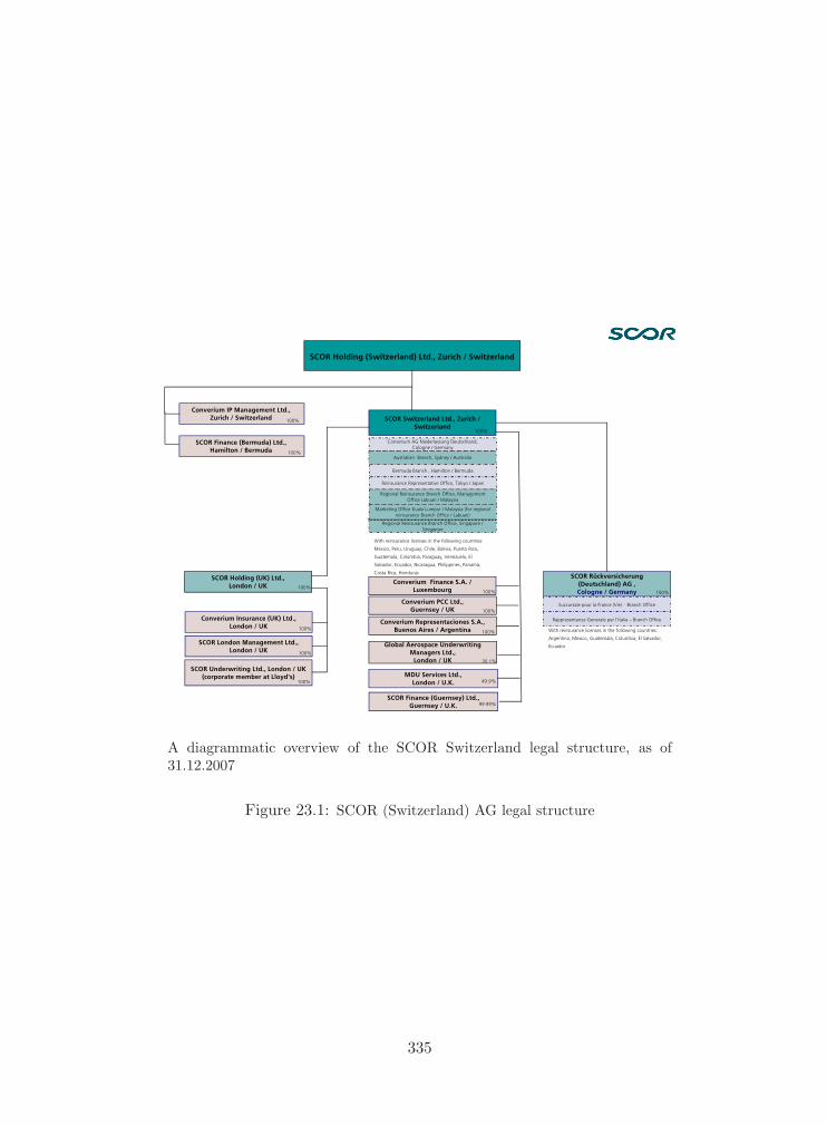
SCOR Holding (Switzerland) Ltd., Zurich / Switzerland
SCOR Finance (Bermuda) Ltd.,Hamilton / Bermuda
Converium IP Management Ltd.,Zurich / Switzerland 100%
100%
SCOR Rückversicherung(Deutschland) AG ,Cologne / Germany 100%
Succursale pour la France (Vie) – Branch Office
With reinsurance licenses in the following countries:
Argentina, Mexico, Guatemala, Columbia, El Salvador,
Ecuador
Rappresentanza Generale per l‘Italia – Branch OfficeConverium Insurance (UK) Ltd.,London / UK
SCOR Underwriting Ltd., London / UK(corporate member at Lloyd‘s)
SCOR London Management Ltd.,London / UK
100%
100%
100%
SCOR Holding (UK) Ltd.,London / UK 100%
SCOR Switzerland Ltd., Zurich / Switzerland
100%
With reinsurance licenses in the following countries:
Mexico, Peru, Uruguay, Chile, Bolivia, Puerto Rico,
Guatemala, Columbia, Paraguay, Venezuela, El
Salvador, Ecuador, Nicaragua, Philippines, Panamá,
Costa Rica, Honduras
Australian Branch, Sydney / Australia
Converium AG Niederlassung Deutschland,Cologne / Germany
Reinsurance Representative Office, Tokyo / Japan
Bermuda Branch , Hamilton / Bermuda
Regional Reinsurance Branch Office, ManagementOffice Labuan / Malaysia
Regional Reinsurance Branch Office, Singapore /Singapore
Marketing Office Kuala Lumpur / Malaysia (for regionalreinsurance Branch Office / Labuan)
Converium Finance S.A. /Luxembourg 100%
Converium Representaciones S.A.,Buenos Aires / Argentina 100%
Converium PCC Ltd.,Guernsey / UK
Global Aerospace UnderwritingManagers Ltd.,
London / UK
100%
MDU Services Ltd.,London / U.K. 49.9%
30.1%
SCOR Finance (Guernsey) Ltd.,Guernsey / U.K. 99.99%
A diagrammatic overview of the SCOR Switzerland legal structure, as of31.12.2007
Figure 23.1: SCOR (Switzerland) AG legal structure
335
2. In August of 2004, in order to retain certain US business, ConveriumAG endorsed for a number of selected cedents of Converium Rein-surance (North America) Inc. a parental guarantee with an optionto novate business written for the 2003 and 2004 underwriting years.Some of these options to novate the business to Converium AG’s bal-ance sheet were executed in the fourth quarter 2004. The remainingcedents did not execute the option and the business remained on Con-verium Reinsurance (North America) Inc.’s balance sheet. Due tothe disposal of Converium’s North American operations to NationalIndemnity Company, Converium AG as the guarantor received fromNational Indemnity Company full indemnification of the potential out-standing liabilities. As of December 31, 2006, 2005 and 2004 theseliabilities were USD 146.1 million, USD 95.7 million and USD 121.4million, respectively.
3. Under the Quota Share Retrocession Agreement with Zurich InsuranceCompany, Converium AG, as at June 30, 2007, bears the credit riskfor potential non-payment of retrocessionaires in the amount of CHF319.6 million. As at December 31, 2006, the potential credit riskstotalled CHF 324.2 million. Exceptions to this to this Quota ShareRetrocession Agreement consist of liabilities that occurred as a resultof the terrorist attacks in the USA on September 11, 2001.
336
24
Fungibility of Capital
The model of capital fungibility is outlined in the internal paper A SimpleModel of Capital Fungibility for Converium ALM by Michel M. Dacorognaand the presentation Fungibility of Capital by Michael Moller presentedto the FOPI. Our documentation on capital fungibility is based on thesematerials (Dacorogna [2007b]).
24.1 Introduction
The purpose of this paper is to give the framework for modeling capitalfungibility in the ALM1. We use the modeling framework suggested by Fil-ipovic and Kupper [2006]. An insurance group with m business units (BU)is considered. Values at the beginning of the period are known and denotedby small letters, while values at the end of the year are random variablesand denoted by capital letters.
We use a coherent measure of risk, ρ, on the probability space E. Wedefine the available capital of BU i as the value of its asset-liability portfolio.We denote by ci ∈ R the capital at the beginning of the year and by Ci ∈ Eat the end of the year. This definition implies the assumption of a valuationprinciple V : E → R such that
ci = V (Ci)
The available capital depends on the selection of liabilities to be covered andthe assets backing these liabilities. We assume here that for each BU therelevant portfolio is determined as it is the case in our new ALM model.
The required capital ki is thus determined by the equation
ki = ci + ρi(Ci)1This part of the documentation deals with the theoretical aspects of internal risk
models. For the details about the ALM and SST processes and the ALM and SST modelingmodules we refer to Part VII.
337
The asset-liability portfolio is considered acceptable if ci > ki.The objective of the group is to account for diversification effects across
the BU’s, which results in an aggregate group required capital, kg, beingless than the sum of the stand-alone BU’s required capitals
kg ≤m∑
i=1
ki
It is understood that the group required capital kg is allocated to the BU’saccording to their (marginal) risk contributions ki
kg =m∑
i=1
ki
24.2 Proposed Framework: Model StandardizedC&R Transfers
We assume that there exists a well-specified finite set of legally enforceablecapital & risk (C&R) transfer instruments with future contingent valuesmodeled by some linearly independent random variables Z0, Z1, . . . , Zn inE. Cash is fungible between BU’s as long as the payments at the end aredetermined at the beginning of the year. This is expressed by letting Z0 ≡ 1.
The modified risk profile of BU i becomes
Ci +n∑
j=0
xjiZj
for some feasible C&R transfer
xi = (x0i , . . . , x
ni ) ∈ Wi, i = 1, . . . , m, (24.1)
such thatm∑
i=1
n∑j=0
xjiZj ≤ 0 (24.2)
where Wi is some closed convex subset in Rn+1 with
0 ∈ Wi and Wi + (r, 0, . . . , 0) = Wi r ∈ R, i = 1, . . . , m.
This means that there is no exogenous value added, because internal riskand capital transfers do not generate positive cash in total. The modifiedrisk profile is solely due to a feasible redistribution of capital and risk bymeans of the instruments Z0, Z1, . . . , Zn.
The aggregate required capital of SCOR Switzerland is
k = c +m∑
i=1
ρi
⎛⎝Ci +
n∑j=0
xjiZj
⎞⎠
338
Lowercase indices i count the legal entities, i.e. i = 1, 2, 3 stand forthe business units Zurich, Cologne, UK, in which case we have m = 3.
Lowercase indices j running from 0 to n index the transfer instru-ments: Cash transfers, internal loans, retrocession programs, parentalguarantees, sale of participations.
xji is the instrument exposure of instrument j of Business Unit i.
Zj is the stochastic portion of instrument exposure j, it equals 1 fordeterministic cash transfers.
Ci is the stochastic available capital of Business Unit i at the end ofthe year without risk transfer.
One task yet to be achieved in the future is to minimize the differencebetween required and available capital. One will have to find an optimalC&R transfer which solves the optimization problem
min(x1,...,xm)
m∑i=1
ρi(Ci +n∑
j=0
xjiZj)
subject to the feasibility and clearing conditions 24.1 and 24.2, respectively.The default risk of guarantors has to be taken into account.
24.3 Application to SCOR (Switzerland) ALM
In our ALM model, we do not directly model the retro but use gross andnet distributions. This, of course, does not allow us to optimize the set ofxi to obtain the best diversification. On the long run, we would like to dothis and would then have to fully model the C&R transfers between thedifferent legal entities. Meanwhile, we can still use the framework withoutoptimization.
For each legal entity, we model the risk gross and net. Because the out-ward retrocession of our company is bought centrally by SCOR SwitzerlandLtd., the difference between gross and net of the other legal entities becomeliabilities of Zurich. For those liabilities that are covered by an outwardretrocession contract, we can assume that they will increase the gross li-abilities but not the net. There are, however, some internal retrocessioncontracts that are not retroceded outside the company, particularly quotashares with London or Cologne. Those will be then direct contributions tothe net liabilities of Zurich and would add to the diversification of the book.
Conversely the economic value of the various legal entities becomes anasset for SCOR Switzerland Ltd. In principle, a Ltd. can sell those legalentities if need be as we have done with Converium North America and
339

realize the economic value of this entity. The economic value of each legalentity owned by SCOR Switzerland Ltd. will thus be added to its availablecapital. In the model implementation, we thus have to add an economicvaluation of each legal entity along the lines of the model we use for theimpairment tests of our yearly balance sheet. Since we have to look at theeconomic view, we cannot simply take the values of the legal entities thatare written on our balance sheet.
In practice, we need to model for each legal entity its own liability grossand net. The difference is then transferred to Zurich. The parental guaranteeoffered by Zurich to Cologne is not modeled by this approach. We need forthis to establish few rules when such a guarantee can be exercised. Wepropose the following two rules:
� The parental guarantee is exercised when the internal retrocession doesnot suffice to assure the solvency of the legal entity.
� The parental guarantee is only exercised when it does not “put indanger” the solvability of the parent. If, for instance, the economiccapital is extinguished or very low so that the likelihood of not ful-filling other obligations becomes high, the seniority of this guaranteemight be subject of juristical debates between regulators and/or otherstakeholders.
With these two rules we set the limit of the capital fungibility vis-a-vis thelegal entities. While the selling of the legal entity establishes the fungibilityin the other direction. We can also add another rule for this direction:
� The legal entity is allowed to transfer capital in favor of the parentonly and only if the amount does not affect the solvability of the legalentity.
With this set of rule, we can have a first approximation of the capitalfungibility. We will be able to measure the efficiency of the fungibility byaggregating the lines of business on the full company and looking at thedifference between the capital needed in aggregate with the capital neededfor the legal entity Zurich modeled as we just described. Of course, wecannot yet optimize the risk transfer between the legal entities as it wouldbe possible if we would fully use the approach proposed in Filipovic andKupper [2006]. We propose to do this in a second step, once we would havegained some experience with the application of this concept. Due to the bigamount of highly liquid invested assets and the ability of transfer of capitalbetween legal entities, it is at the moment assumed that liquidity risk is ofminor importance for SCOR Switzerland.
340

24.4 Limitations of Modeling of CapitalFungibility
In case of financial distress of both the parent and a potential subsidiary inanother country it is not clear to what extend the different regulators wouldlimit the allowance of capital transfers.
341

25
The Valuation of Assets
The SST regulations propose a standard which evaluates assets generally atmarket conditions (economic valuation). The statement of the company’sfinancial condition and the report on the value of the company’s assets at agiven point in time rely on the determination of the fair value of the com-pany’s assets where the notion of fair value refers to the price, expressed incash equivalents, at which property is exchanged between the seller and thebuyer in an open and unrestricted market1. The company’s banking partnersprovide sufficient information to directly determine, for example, the amountof cash, equities and bonds and also the market value of derivative financialmarkets instruments, like swaptions (Iannuzzi [2007]) at t0. These marketvalues constitute an essential part of the initial economic balance sheet andthe valuation is typed mark to market. There are classes of assets, however,which equally influence the company’s financial position yet will not be readoff the company’s bank accounts or are not traded in a deep and liquidmarket from where reliable and comparable market prices are available. Anincome approach may then be the most logical and most practical techniqueto estimate the fair value, by assessing the net present value2 (NPV) of thebenefit stream of cash flows generated by the business. The NPV basedvaluation illustrates the mark to model approach with its contingency onthe realism of financial model assumptions. As an illustration, the intrinsicvalue of SCOR Switzerland’s funds withheld assets is NPV based. With
1In the absence of an actual exchange the fair value is a hypothetical price contingenton the assumptions about an idealized market. It is an estimate of the price at whichassets or liabilities could be exchanged in transaction between knowledgeable, unrelated,willing parties.
2The NPV, defined as the discounted excess of cash flows, i.e. discounted benefitcash flows minus the initial capital outlay, specifies one distinct approach towards thedetermination of a fair value. We emphasize that various classes of our company’s assetsare valued by SCOR Switzerland’s banking partners, based on their own specialized modelsand the specific knowledge by these institutions. At this point we do not indicate anythingabout these methods which may of course deviate from an idealized NPV valuation or maybe based on adequate principles other than an NPV valuation in the narrow sense.
342

complex financial instruments, marking to model is the only applicable val-uation method. SCOR Switzerland holds structured notes (Iannuzzi [2007])specifically designed to protect the company’s balance sheet against interestrate (IR) risk. There is no established market for these hedges as they areissued by banking partners (Hypo Vereinsbank, Germany) exactly for thatpurpose. The issuer combines the available market data into a market val-uation which is finally reported to the global custodian (Mellon Bank, NewYork) from where, in turn, it indirectly enters the company’s balance sheet.
The issuers of financial instruments as well as the banking institutionswhich are responsible for safeguarding3 the company’s financial assets reg-ularly provide relevant, reliable and comparable values on the company’sassets. They report the asset classes and the actual value of assets whichserve as the starting point for stochastic simulation and for risk evaluation(see, for instance, economic scenario generation in Chapter 10 and creditrisk, Part III).
In the real estate market an intricate aggregation of estimates is usedby real estate fund managers for real estate appraisal, where different values(comparable sales, replacement costs, income approach: value in use) mustbe read against each other and are aggregated over a wide variety of indi-vidual assets4. Fair values, as obtained by fund managers and also througha third party are once more registered by the global custodian.
SCOR Switzerland is holding shares in real estate investment trustswhich are quoted on a stock exchange. These values are therefore marketvalues.
Table 25.1 lists the classes of assets held by SCOR Switzerland. It spec-ifies the valuation methods by which corresponding fair or mark-to-modelvalues are assigned to them.
The required valuation at the end of the year, i.e. the contribution to the1% expected shortfall of the economic value of the company, of most investedassets is based on the mapping of the returns of the economic scenariogenerator5 to the investment classes mentioned above. The handling of theaccounting of the invested assets and the cash flows stemming from theinsurance business is discussed in Part II.
Real Estate
SCOR Switzerland holds shares of the Morgan Stanley Euro Zone OfficeFund, a private equity fund for institutional investors6. Audited funds re-
3Most notably invested fixed maturity assets: Bank of New York Mellon, Asset Services,Global Custody.
4Again, the simplified nature of this example shall merely serve the purpose of illus-tration and shall not be applicable to infer the actual methods and assumptions used forvaluation by the real estate fund managers.
5For the details of economic scenario generation see Chapter 10 of this documentation.6SCOR Switzerland keeps its shares below 20%.
343

Assets Valuation
Invested AssetsFixed maturities Marked to marketFunds withheld Marked to model (NPV based)Investments in subsidiaries Marked to modelEquity securities Marked to marketDerivatives (interest rate hedges) Marked to model (by banking
partners)Real estate Marked to modelShort term investments and otherinvestments
Marked to market
Other assetsCash and cash equivalents Marked to marketPremiums receivable Marked to model (NPV based
for best estimate)Underwriting reserves, retrocession Marked to model (NPV based
for best estimate)Funds held by reinsureds Marked to modelDeposit assets Not material, treated as funds
held by reinsuredsInsurance and reinsurance balancespayable and other reinsurance re-ceivables
Not yet fully modeled
Deferred policy acquisition costsand deferred income taxes
Set to zero
Reserves for unearned premiums,retrocession
Marked to model.
Derivatives Marked to market (by bankingpartners)
Other assets and accrued income Not yet modeled
Table 25.1: The classes of assets and their mode of valuation.
344
porting is done as of end of year. It’s based on a third party assessmentof the value. Quarterly evaluation and reporting is performed by the funditself. The fair value, based on the quarterly numbers, is reported by to theglobal custodian (Mellon Bank, N.Y.). The entire process is accompaniedby adequate SarbOx checks. The valuation at the end of the year is basedon the simulation of real estate returns of the economic scenario generator.
Derivative Instruments, Hedge Funds, Registered Bonds
Market values of structured notes and registered bonds held by SCOR Switzer-land are reported by the deposit banks to the custodian (Mellon Bank, N.Y.).Hedge funds report to the custodian (Mellon Bank, N.Y.) on a monthly ba-sis.
� Digital Notes are non listed assets, with variable returns and a fixednotional (Iannuzzi [2007], see Chapter 11). The issuing banking insti-tution (Hypo Vereinsbank, Germany) reports the fair values to MellonBank.
� Registered bonds are in the books of SCOR Switzerland (Cologne),these are non listed securities the fair value of which is calculated bythe custodian banking institution (Commerzbank, Germany). SCORSwitzerland (Cologne) reports these values to it’s global custodian(Mellon Bank).
� The performance of hedge funds is closely monitored and the invest-ment department as well as the custodian, Mellon Bank, receive monthlyreports from the global hedge fund managers.
The analyzes and reports of Mellon Bank on these securities are regularlymonitored by SCOR Switzerland. The end of year valuation of these assetsis modeled in SCOR Switzerlands simulation model. On the derivative side,the Black Scholes formula using ESG-input is used for valuing the swaptions.Structured notes are valued by building a linear interpolation of a functionof the ESG-generated interest rate curve. ESG-returns from Hedge FundIndices are used to simulate the value of the Hedge Funds at year-end.
Participation
The value of a participation as invested asset at t0 equals the economic valueof the subsidiary valued by SST principles, i.e. computed as market value ofthe assets less best estimate of the liabilities of this subsidiary. As we fullymodel our major subsidiaries (Cologne and UK) we compute the impact ofthe simulated values of the participation given the worst 1% scenarios of theparent at the end of the year. The average of these values is taken as theexpected value of the participation at the end of the year. Other subsidiaries
345

with non-material value are taken as constants with their financial balancesheet value.
Other Assets
Deferred policy acquisition costs. These are acquisition costs prin-cipally representing commissions and brokerage expenses, premium taxesand other underwriting expenses, net of allowances from retrocessionaires,which vary with and are directly related to the production of new business,are deferred and amortized over the period in which the related premiumsare earned7. The DAC-position is generally set to zero as the – economicallyrelevant – cash outflows happened in the past. (The calculation of futureincome would contain the related deferred costs but this is only of theoreti-cal interest as the SST-relevant future cash flows belonging to the businessare just not lowered by the acquisition costs paid in the past.)
Reinsurance Assets. These are valued like reserves (see Chapter 3)except that they are also associated with a credit risk discount (see PartIII). The credit risk due to the potential default of the retrocessionaire ismodeled like the credit risk of a bond with similar rating and duration.
Funds Held by Reinsureds. The valuation of funds held by rein-sureds is based on the NPV of the associated cash flows and a small creditrisk (as these funds are partially hedged by related reserve positions). Thecredit risk related to the non-hedged part of the funds is modeled in thesame way as the credit risk of the reinsurance assets.
7Converium annual report 2006, p. 71.
346
26
The Valuation of Liabilities
In the following, the valuation of the major liability items are outlined. Thisrelates mainly to reserves, funds held under reinsurance contracts, payablesand debt which are valued at best estimate (MVM is treated separately)at the beginning of the year and as the contribution to the 1% expectedshortfall of the economic value of the company at the end of the year. (Themodeling of the stochastic behavior of the liability risk is outlined in chapter2.) Generally, the valuation of liabilities contains the market value mar-gin which are the costs of capital associated with the necessary capital forkeeping the run-off portfolio after one year. Table 26.1 lists the classes ofliabilities and their valuation without the market value margin. The calcu-lation of the MVM is also documented in detail in chapter 2.
Reserves
The valuation of the reserves at t0 is done at their best estimate. At theend of the year, based on the stochastic simulation result of the reservedevelopment, the contribution to the expected shortfall of the value of thecompany is considered, see Chapter 3 for a comprehensive analysis of thevaluation of reserves, their volatility and development over time. Clearly,the MVM is mainly related to the cost of capital associated with the capitalneeded to cover the future volatility of the run-off reserves after one year.
Unearned Premium Reserves
The risk associated with unearned premium reserves is modeled on the basisof the new business loss distribution per line of business. Consequently, thevaluation of this position is relying on the NPV of the expected value (fort0) and the contribution to the expected shortfall to the economic value ofthe legal entity at the end of the year.
347

Liability Valuation
Underwriting reserves (gross) Marked to model (best esti-mate: discounted reserves)
Insurance and reinsurance balancespayable
Marked to model
Reinsurance liabilities (retro) Marked to model (NPV basedfor best estimate)
Life Marked to modelReserves for unearned premium(gross)
Marked to model
Other reinsurance liabilities Not yet modeledCeded premiums payable Marked to model (NPV based
for best estimate)Funds held under reinsurance con-tracts
Marked to model (NPV basedfor best estimate)
Deposit liabilities Not yet modeledDeferred income taxes Excluded from market consis-
tent balance sheet (not mate-rial anyway)
Other liabilities and accrued ex-penses
Marked to model
Debt/loans Face valueOptions and guarantees Off balance sheet, modeled in
liability cash flows
Table 26.1: The liabilities and their mode of valuation.
348

Funds Held under Reinsurance Contracts
These funds are valued on an NPV cash flow basis using related cash flowpatterns.
Debt
Ordinary issued debt is in general valued like a corporate bond, see Parts II,III and especially Chapter 12 for market risk, credit risk and bond valuation.To the extent these debts are subordinated they are considered as part of
the capital basis. This means that their face value must be usable in case offinancial distress and can not trigger the liquidation of the company (whichis tested during the simulations). It is especially important that these debtsare subordinated relative to the payments to policyholders.
Payables
This position is valued on an NPV cash flow basis using (short-term) cashflow patterns.
Other reinsurance liabilities, Pension liabilities
These liabilities currently comprise roughly 1.2% of SCOR Switzerlands li-abilities and are not yet fully modeled in detail. A smaller fraction (30%)of these liabilities are currently related to pension liabilities to be paid toSCOR Switzerlands employees (a small part of the pension liabilities arereported as loss in “Other comprehensive income”) by SCOR Switzerland.This is basically the gap between the projected benefit obligations and thefair value of the plan assets of the pension fund, adjusted by the tax impact.
Off-Balance Sheet items
Embedded value of life insurance The valuation of the embeddedvalue of life insurance business equals the NPV of the expected economiclife-insurance related cash flows for t0 and the contribution to the expectedshortfall to the economic value of the legal entity at the end of the year. Op-tions and guarantees are explicitly simulated in related models, see chapter4.
CRTI, credit lines, contingent capital The impact of capital andrisk transfer instruments on the valuation of the legal entity is directly simu-lated using information on parental guarantees or the retro structure. Con-tingent capital is negligible for SCOR Switzerland. Non collateralized Let-ters of credit are assumed to positively impact the policyholders’ interestbut is not supposed to alter the economic value of the legal entity.
349

VI
Solvency CapitalRequirements
350
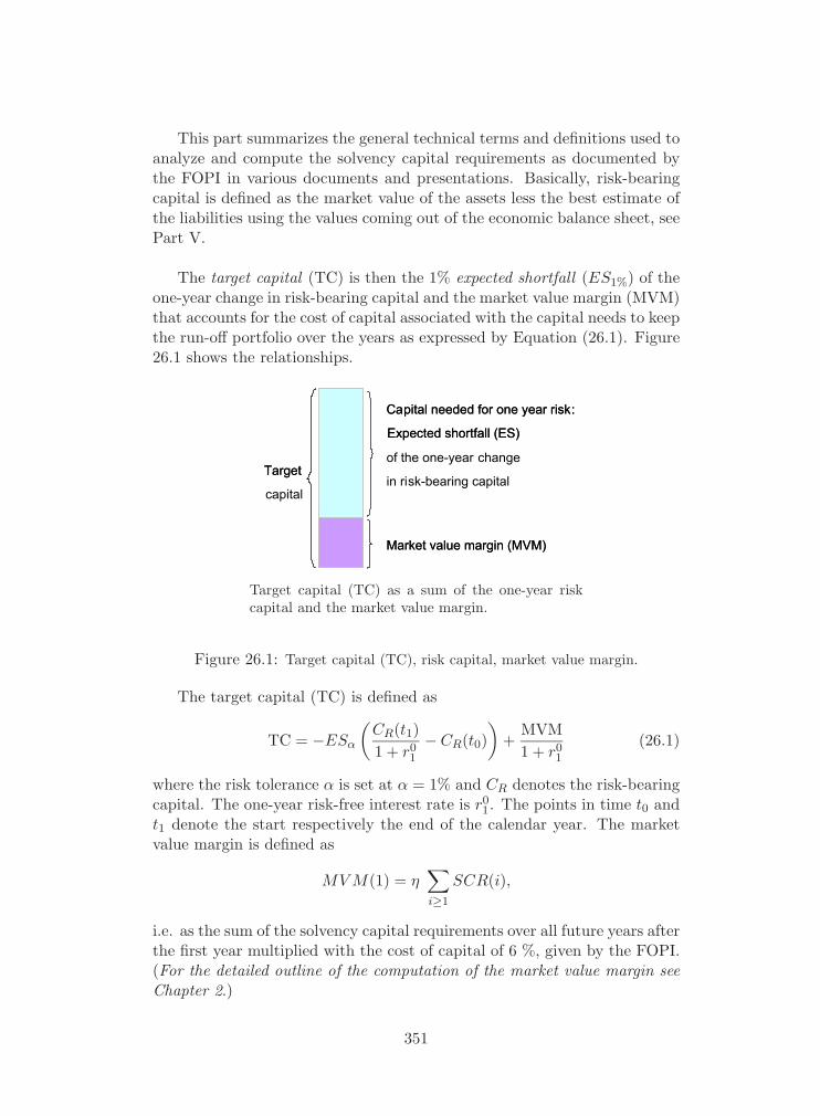
This part summarizes the general technical terms and definitions used toanalyze and compute the solvency capital requirements as documented bythe FOPI in various documents and presentations. Basically, risk-bearingcapital is defined as the market value of the assets less the best estimate ofthe liabilities using the values coming out of the economic balance sheet, seePart V.
The target capital (TC) is then the 1% expected shortfall (ES1%) of theone-year change in risk-bearing capital and the market value margin (MVM)that accounts for the cost of capital associated with the capital needs to keepthe run-off portfolio over the years as expressed by Equation (26.1). Figure26.1 shows the relationships.
Target
capital
Capital needed for one year risk:
Expected shortfall (ES)
of the one-year change
in risk-bearing capital
Market value margin (MVM)
Target
Capital needed for one year risk:
Expected shortfall (ES)
Market value margin (MVM)
Target capital (TC) as a sum of the one-year riskcapital and the market value margin.
Figure 26.1: Target capital (TC), risk capital, market value margin.
The target capital (TC) is defined as
TC = −ESα
(CR(t1)1 + r0
1
− CR(t0))
+MVM1 + r0
1
(26.1)
where the risk tolerance α is set at α = 1% and CR denotes the risk-bearingcapital. The one-year risk-free interest rate is r0
1. The points in time t0 andt1 denote the start respectively the end of the calendar year. The marketvalue margin is defined as
MV M(1) = η∑i≥1
SCR(i),
i.e. as the sum of the solvency capital requirements over all future years afterthe first year multiplied with the cost of capital of 6 %, given by the FOPI.(For the detailed outline of the computation of the market value margin seeChapter 2.)
351

VII
Process Landscape
352
Table of Contents
27 Summary 358
28 Structure of the Process Landscape Documentation 360
29 Overview 362
29.1 The Swiss Solvency Test / Asset and Liability ManagementProcess . . . . . . . . . . . . . . . . . . . . . . . . . . . . . . 362
29.1.1 Process Description . . . . . . . . . . . . . . . . . . . 363
29.1.2 Roles and Responsibilities . . . . . . . . . . . . . . . . 364
29.2 General Timeline of the SST and the ALM Process at SCORSwitzerland . . . . . . . . . . . . . . . . . . . . . . . . . . . . 366
29.3 Q3 ALM process . . . . . . . . . . . . . . . . . . . . . . . . . 366
29.4 Q1 ALM process . . . . . . . . . . . . . . . . . . . . . . . . . 367
30 The ALM Process 368
30.1 General Overview . . . . . . . . . . . . . . . . . . . . . . . . . 368
30.2 The Execution of the ALM Model . . . . . . . . . . . . . . . 369
30.2.1 Roles and Responsibilities . . . . . . . . . . . . . . . . 370
30.3 Detailed Module Description . . . . . . . . . . . . . . . . . . 371
30.3.1 The Economic Scenario Generator . . . . . . . . . . . 371
30.3.2 Reserve Modeling . . . . . . . . . . . . . . . . . . . . . 376
30.3.3 Liability Modeling . . . . . . . . . . . . . . . . . . . . 380
30.3.4 Asset Modeling . . . . . . . . . . . . . . . . . . . . . . 389
30.3.5 Aggregated Results Calculation . . . . . . . . . . . . . 393
31 Scenarios 397
31.1 Overview . . . . . . . . . . . . . . . . . . . . . . . . . . . . . 397
31.2 Process Steps . . . . . . . . . . . . . . . . . . . . . . . . . . . 398
353

31.3 Roles and Responsibilities . . . . . . . . . . . . . . . . . . . . 399
31.4 Sign-off Procedures . . . . . . . . . . . . . . . . . . . . . . . . 401
32 Appendix 402
32.1 Sign-off Matrix . . . . . . . . . . . . . . . . . . . . . . . . . . 402
32.1.1 Timeline of Project . . . . . . . . . . . . . . . . . . . . 402
32.1.2 Project – Sign-off Matrix . . . . . . . . . . . . . . . . 403
32.1.3 Project Roles and Responsibilities . . . . . . . . . . . 403
32.1.4 Project Organizational Overview of Roles and Respon-sibilities . . . . . . . . . . . . . . . . . . . . . . . . . . 405
354

List of Tables
31.1 Scenario production process – sign-off matrix. . . . . . . . . . . . 401
32.1 SST project – sign-off matrix. . . . . . . . . . . . . . . . . . . . 403
355
List of Figures
29.1 Embedment of the ALM process at SCOR Switzerland – organiza-tional overview. . . . . . . . . . . . . . . . . . . . . . . . . . . . 362
29.2 The SST and the ALM process at SCOR Switzerland – generaltimeline. . . . . . . . . . . . . . . . . . . . . . . . . . . . . . . 367
30.1 ALM process – functional overview. . . . . . . . . . . . . . . . . 368
30.2 ALM process – modules. . . . . . . . . . . . . . . . . . . . . . . 369
30.3 ALM process – economic scenario generator. . . . . . . . . . . . . 371
30.4 ALM process – reserve modeling. . . . . . . . . . . . . . . . . . . 376
30.5 ALM process – liability modeling. . . . . . . . . . . . . . . . . . 380
30.6 ALM process – asset modeling. . . . . . . . . . . . . . . . . . . . 389
30.7 ALM process – aggregated results calculation. . . . . . . . . . . . 393
31.1 Scenario production process. . . . . . . . . . . . . . . . . . . . . 397
32.1 Timeline to implement the SST at SCOR Switzerland. . . . . . . . 403
32.2 Organizational overview of roles and responsibilities. . . . . . . . . 406
356

Abbreviations
ALM Asset and Liability ManagementBoD Board of DirectorsBS Balance SheetCEO Chief Executive OfficerCFO Chief Financial OfficerCIO Chief Investment OfficerCOO Chief Operating OfficerCPI Consumer Price IndexCRO Chief Risk Officerdvlpmt. developmentECS Executive Committee SwitzerlandESG Economic Scenario GenerationEUR EuroFED Financial and Economic DatabaseFinMod Financial ModelingFOPI Federal Office of Private InsuranceFX EffectsGAUM Global Aerospace Underwriting ManagersGDP Gross Domestic ProductGMDB Guaranteed Minimum Death BenefitLoB Lines of BusinessMDU Medical Defense UnionMgmt. ManagementMVM Market Value MarginNat Cat Natural CatastrophesNon-prop. Non-proportionalProp. ProportionalQ1 First quarterQ3 Third quarterRBC Risk Based CapitalS&P Standard & PoorsSST Swiss Solvency Teststrat. strategicUSD US dollarUWY Underwriting Year
357

27
Summary
The ultimate objective of the Swiss Solvency Test (SST) is to determinea company’s solvency status, using an all encompassing analysis of therespective company. The main ideas of the SST are described in the SSTWhite Paper (FOPI [2004]) issued by the FOPI. In the past, SCOR Switzer-land used its internal stochastic model to manage assets and liabilities.This model has now been enhanced and expanded to include all SST rele-vant aspects and elements. Going forward, the internal model will be usedfor both asset and liability and solvency calculations for the purposes of theSST.
The SST is of great relevance for the management decision processesat SCOR Switzerland. With our internal stochastic models we calculateresults on an ultimate basis for the Asset and Liability Management (ALM)and on a one year basis for the SST. These results define such business rele-vant issues as the group’s strategic asset allocation, the exposure of thegroup to main risk classes or the capital requirements needed. Addi-tionally, a forecast of the asset performance is provided. These results serveas guidance for the group’s risk appetite and risk mitigation, the as-set management strategy and the capital management. The internalmodel therefore passes the requirements of a use test.
From the viewpoint of the process documentation we understand theSST as a use test. The main purpose is to show the processes of how we getto the SST relevant results. Our internal stochastic models serve as thestarting point for the ALM. Preparing for the SST, we enhanced our ALMprocess to be fully inline with the SST requirements, set up by the FederalOffice of Private Insurance (FOPI). The SST is therefore closely linkedto the ALM process.
The ALM process at SCOR Switzerland is specified by five process
358

modules: “economic scenario generation,” “reserving,” “asset management,”“liability management” and “aggregated results calculation.” This documentprovides a detailed description of input-to-output processes within the sin-gle modules. Insurance risk, market risk, and credit risk modeling arecarried out with specific focuses in these modules.
The SST process documentation is an integral part of the supportingdocumentation produced and submitted to the FOPI:
� The design of the ALM modules and the process steps in particularare based on the ideas as highlighted in the SST White Paper (FOPI[2004]) issued by the FOPI.
� The high-level dataflows and process steps as specified in the modulesof the ALM process form the basis for the IT Systems documentation(Part VIII, pp. 408).
� The methodology used for the calculation is described in this docu-mentation (see, above all, the Parts I, II, III in this document).
359
28
Structure of the ProcessLandscape Documentation
The documentation of the process landscape at SCOR Switzerland Ltd. isbased on Swiss Solvency Test (SST) at SCOR Switzerland: Process Land-scape (Skalsky and Burgi [2008]) and is structured as follows:
We first give an overview of the embedment of the ALM process withinSCOR Switzerland. The SST is performed based on the results from theALM process. The overview includes a comprehensive description of rolesand responsibilities and the decision processes related to the results ofthe SST and the ALM Report. This first part shows that the ALM processis an integral part of the overall company processes.
We subsequently describe the ALM process in detail. It is structuredin modules which are combined to workflows. Each module consists of anumber of input and output data entities as well as a number of pro-cess components. The roles and responsibilities are defined by module,and for the output data entities, the corresponding sign-off proceduresare described.
We then provide an overview of the process of creating the scenariosused for the SST only. The main purpose of this section is to show thegeneral process steps that are performed every year to decide upon therelevance of the used scenarios and, if necessary, the production of newscenarios needed. This part mainly refers to the detailed scenario docu-mentation (Gencyilmaz [2007]), provided to FOPI on a yearly basis as anintegral part of the SST Report.
In the Appendix, a general overview of the SST project setup, the time-line of implementation, as well as the project roles and responsibilities and
360

the sign-off matrix of the overall project is presented. The SST project hasthe goal to achieve SST compliance of SCOR Switzerland and to implementmethods and processes in order to satisfy the FOPI requirements.
361
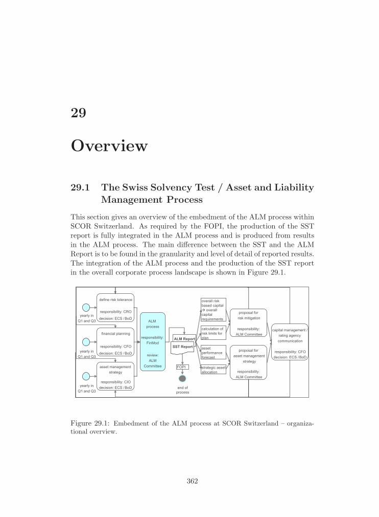
29
Overview
29.1 The Swiss Solvency Test / Asset and LiabilityManagement Process
This section gives an overview of the embedment of the ALM process withinSCOR Switzerland. As required by the FOPI, the production of the SSTreport is fully integrated in the ALM process and is produced from resultsin the ALM process. The main difference between the SST and the ALMReport is to be found in the granularity and level of detail of reported results.The integration of the ALM process and the production of the SST reportin the overall corporate process landscape is shown in Figure 29.1.
define risk tolerance
responsibility: CRO
decision: ECS / BoD
financial planning
responsibility: CFO
decision: ECS / BoD
yearly in Q1 and Q3
proposal for risk mitigation
responsibility: ALM Committee
asset management strategy
responsibility: CIOdecision: ECS / BoD
overall risk based capital
overall capitalrequirements
calculation of risk limits for plan
FOPI
end of process
asset performance forecast
strategic asset allocation
proposal for asset management
strategy
responsibility: ALM Committee
capital management / rating agency communication
responsibility: CFOdecision: ECS / BoD
yearly in Q1 and Q3
yearly in Q1 and Q3
ALM Report
SST Report
ALMprocess
responsibility: FinMod
review:ALM
Committee
Figure 29.1: Embedment of the ALM process at SCOR Switzerland – organiza-tional overview.
362

29.1.1 Process Description
Processstep
Description
Assetman-agementstrategy
The asset management strategy covers strategic assumptionson
� The proportion of asset classes (e.g. fixed income vs.equity vs. other financial products)
� The target duration of bonds
The Chief Investment Officer is responsible to define theasset management strategy. The asset management strategyis approved by the ECS and the BoD.
ALMprocess
The ALM process takes the risk tolerance, the financial plan,and the asset management strategy as an input. The mainproducts of the process are the ALM report and the SSTreport. The results listed in these reports cover
� The exposure of the group to the main risk classes
� The overall capital requirements needed given the planand the asset management strategy
� A forecast of the asset performance
� A proposal for the strategic asset allocation
The overall responsibility of the ALM process lies with theFinancial Modeling team. The results of the SST and theALM Report are approved by the ALM Committee. Fur-thermore, the ALM Committee decides on proposals for riskmitigation and asset management strategy.
Proposalforrisk mit-igation
If the overall capital requirements or the risk components ascalculated by the ALM process violate the risk tolerance ofthe group, the risks have to be mitigated or the risk toler-ance has to be redefined. The ALM process comes up witha suggestion for risk mitigation, which is proposed to theBoD/ECS. Depending on the outcome, the risk tolerance,the financial plan or the asset management strategy mayhave to be revised.
363
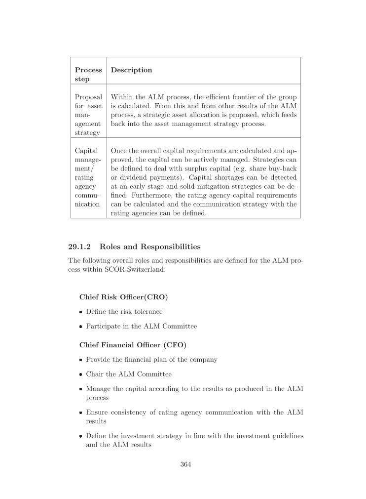
Processstep
Description
Proposalfor assetman-agementstrategy
Within the ALM process, the efficient frontier of the groupis calculated. From this and from other results of the ALMprocess, a strategic asset allocation is proposed, which feedsback into the asset management strategy process.
Capitalmanage-ment/ratingagencycommu-nication
Once the overall capital requirements are calculated and ap-proved, the capital can be actively managed. Strategies canbe defined to deal with surplus capital (e.g. share buy-backor dividend payments). Capital shortages can be detectedat an early stage and solid mitigation strategies can be de-fined. Furthermore, the rating agency capital requirementscan be calculated and the communication strategy with therating agencies can be defined.
29.1.2 Roles and Responsibilities
The following overall roles and responsibilities are defined for the ALM pro-cess within SCOR Switzerland:
Chief Risk Officer(CRO)
� Define the risk tolerance
� Participate in the ALM Committee
Chief Financial Officer (CFO)
� Provide the financial plan of the company
� Chair the ALM Committee
� Manage the capital according to the results as produced in the ALMprocess
� Ensure consistency of rating agency communication with the ALMresults
� Define the investment strategy in line with the investment guidelinesand the ALM results
364

Chief Investment Officer (CIO)
� Define the asset management strategy based on ALM results
� Sign-off on the investment forecasts as produced in the ALM process
� Participate in the ALM Committee
Financial Modeling (FinMod)
� Manage the ALM process overall
� Create and validate appropriate models
� Produce the various calculation results (for the ALM as well as for theSST report)
� Achieve a sign-off from the relevant parties
� Ensure that the ALM results are appropriately dealt with
� Secretary of the ALM Committee
� Reporting of the ALM results to ECS and BoD
ALM Business Owner
� Ensures that the end product is fit for its purpose and that the solutionwill meet the user/business needs within the constraints of the businesscase,
� Provides business resources and must be of sufficient authority to takedecisions on business matters
� Ultimate responsibility for sign-off on the projects products
Local Chief Risk Officer
� Produce the SST report
� Obtain sign-off of the SST report
� Publish the SST report and submit it to the FOPI
365
ALM Committee
� Sign-off on adequacy of models and results
� Propose the strategic asset allocation to ECS and BoD
� Propose an investment strategy based on the ALM results
� Propose risk mitigation strategies as needed based on the ALM results
� Ensure that the ALM results are reflected in related decisions of thecompany
� Publication of the ALM report – sign-off and publication of the SSTreport
Executive Committee Switzerland and Board of Directors(ECS/ BoD)
� Decide on the risk tolerance
� Agree on the strategic asset allocation
� Decide on the investment strategy,
� decide on risk mitigation if necessary
� Decide on capital management
29.2 General Timeline of the SST and the ALMProcess at SCOR Switzerland
The ALM process is carried out twice a year within SCOR Switzerland. TheSST is performed once a year, based on the ALM calculations in Q1. A highlevel overview is given in Figure 29.2.
29.3 Q3 ALM process
The Q3 ALM process starts in September and ends in December. Its purposeis to forecast results of the next financial year based on the financial planof the company, which is based on the risk tolerance defined. The ALMprocess is carried out as described below.
The capital requirements are calculated, and the risk limits are moni-tored. If the financial plan violates the risk tolerance, it has to be revised.
366

calculate assets & liabilities
perform Swiss Solvency
Test (SST)
yearly in Q3
compareresults from Q3 with Q1 results
Reconcile any
differences
end of process
end of processreview
financial Planningfor the
year
calculate assets &liabilities
fix financial planningfor next
year
review risk tolerance
yearly in Q1
3QALM
Report
1QALM
Report
SST Report
yearly in Q3
Figure 29.2: The SST and the ALM process at SCOR Switzerland – generaltimeline.
29.4 Q1 ALM process
The Q1 ALM process starts in March and ends in July. Based on the resultsof the renewals to date and based on the investment results to date, the fore-cast of the Q3 ALM process are refined to reflect the actual developments.
The Q1 ALM results are parsed to the SST Report. Additionally, thesections specific to the SST report only are produced. The SST Report issubmitted to the FOPI.
367
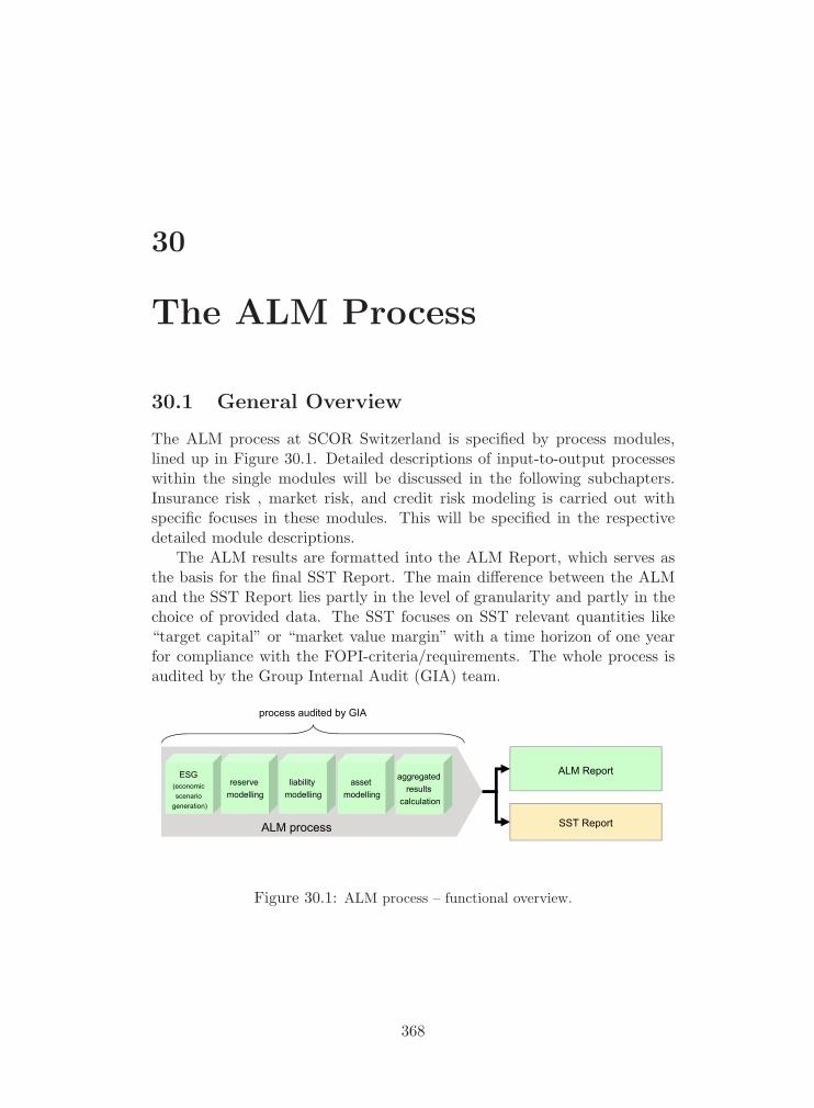
30
The ALM Process
30.1 General Overview
The ALM process at SCOR Switzerland is specified by process modules,lined up in Figure 30.1. Detailed descriptions of input-to-output processeswithin the single modules will be discussed in the following subchapters.Insurance risk , market risk, and credit risk modeling is carried out withspecific focuses in these modules. This will be specified in the respectivedetailed module descriptions.
The ALM results are formatted into the ALM Report, which serves asthe basis for the final SST Report. The main difference between the ALMand the SST Report lies partly in the level of granularity and partly in thechoice of provided data. The SST focuses on SST relevant quantities like“target capital” or “market value margin” with a time horizon of one yearfor compliance with the FOPI-criteria/requirements. The whole process isaudited by the Group Internal Audit (GIA) team.
ALM process
ESG(economicscenario
generation)
reservemodelling
liabilitymodelling
assetmodelling
aggregatedresults
calculation
ALM Report
SST Report
process audited by GIA
Figure 30.1: ALM process – functional overview.
368

30.2 The Execution of the ALM Model
This chapter describes the process of executing the ALM model. This pro-cess encompasses
� The collection of all relevant data entities
� The re-modeling of some of these data entities in order to match thedesired level of granularity and aggregation
� The calculation of the overall result distribution as well as risk mea-sures, strategic asset allocation etc. as desired by the various stake-holders (management, regulators, rating agencies etc)
The ALM model execution process is structured in five modules whichare represented as a workflow in Figure 30.2.
ESG(economicscenario
generation)
reservemodelling
liabilitymodelling
assetmodelling
aggregatedresults
calculation
ALM process
Figure 30.2: ALM process – modules.
In summary, the scope of the modules can be described as follows:
Economic scenario generation: A forecast of the world economyis generated in the form of various economic scenarios and their respectiveprobabilities. Historic time series serve as input and are projected to thefuture.
Reserve modeling: The starting point of the reserve model are thefigures contained in the balance sheet. Based on reserving triangles (claimsincurred, claims paid, premiums received etc.), patterns are determined andthe reserve volatility is calculated.
Liability modeling: The loss models of single acceptances or line ofbusiness fragments are gathered and aggregated. The dependency structureis modeled. The loss models are projected to the planning figures. The grossliability cash flows are calculated by year, legal entity and line of business.Internal and external retro is deducted to generate net cash flows.
369

Asset modeling: The asset portfolio is stylized in order to reduce thecomplexity of the calculations. Similar assets are gathered to asset classes.The asset management – module delivers results for the invested assets per-formance, stand-alone risk-based capital, sensitivity of invested assets andthe efficient frontier analysis, which is a core result of the ALM process. Theefficient frontier graph sets the expected shortfall in relation to sharehold-ers equity and compares SCOR Switzerland’s asset portfolio with the mostefficient strategic asset allocation.
Aggregated results calculation: The aggregated results calculationmodule is the last module in the ALM process. It calculates the main resultsneeded for capital management and the Swiss Solvency Test.
30.2.1 Roles and Responsibilities
Two roles with an overall coordinative function are specified in general termsfor the ALM and SST processes. Roles and responsibilities of the ALM andSST process managers are defined:
ALM process manager
� Plan the process and manage changes
� Nominate persons to the defined roles and responsibilities, includingthe nomination of the respective deputy functions
� Progress monitoring and reporting
� Manage process definitions
SST process manager
� Produce the SST report from results of the ALM report
� Obtain a sign-off of the SST report from the ALM Committee
� Submit the SST report to the FOPI
370
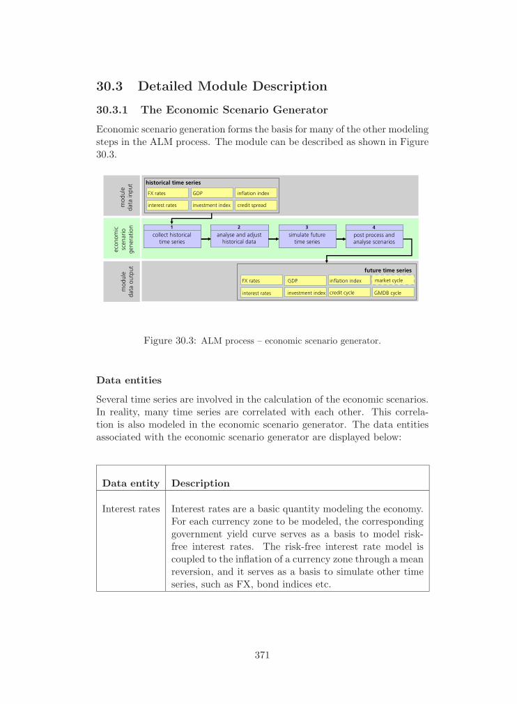
30.3 Detailed Module Description
30.3.1 The Economic Scenario Generator
Economic scenario generation forms the basis for many of the other modelingsteps in the ALM process. The module can be described as shown in Figure30.3.
1
collect historicaltime series
2
analyse and adjusthistorical data
3
simulate futuretime series
4
post process andanalyse scenarios
1
collect historicaltime series
2
analyse and adjusthistorical data
3
simulate futuretime series
4
post process andanalyse scenarios
1
collect historicaltime series
2
analyse and adjusthistorical data
3
simulate futuretime series
4
post process andanalyse scenarios
FX rates
interest rates
GDP
investment index
inflation index
credit spread
historical time series
econ
omic
scen
ario
gene
ratio
n
FX rates
investment index
GDP
credit cycle
inflation index
GMDB cycle
future time series
mod
ule
data
inpu
tmod
ule
data
output
interest rates
market cycle
Figure 30.3: ALM process – economic scenario generator.
Data entities
Several time series are involved in the calculation of the economic scenarios.In reality, many time series are correlated with each other. This correla-tion is also modeled in the economic scenario generator. The data entitiesassociated with the economic scenario generator are displayed below:
Data entity Description
Interest rates Interest rates are a basic quantity modeling the economy.For each currency zone to be modeled, the correspondinggovernment yield curve serves as a basis to model risk-free interest rates. The risk-free interest rate model iscoupled to the inflation of a currency zone through a meanreversion, and it serves as a basis to simulate other timeseries, such as FX, bond indices etc.
371
Inflationindex
The inflation in a currency zone is another importantquantity modeling basic economic behavior. The con-sumer price index (CPI) is taken as a measure for in-flation. Inflation and interest rates are coupled through amean reversion. Furthermore, the inflation has an impacton FX rates and equity indices modeled.
FX rates The FX rates are defined with respect to the home cur-rency (USD for SCOR Switzerland, EUR for SCOR). TheFX rate model depends on the risk free interest rates aswell as on the inflation of the corresponding currency zoneand of the home currency zone.
GDP The modeling of the gross domestic product is indepen-dent of other variables of the economy. However, the mod-eled GDP is used to model investment indices.
Investmentindex
Investment indices are typically equity indices, bond in-dices, real estate indices, hedge fund indices or similar.The modeling of investment indices depends on other ba-sic quantities such as the inflation and the GDP or interestrates of a currency zone. The investment indices are usedto valuate the asset portfolio in the risk simulation.
Creditspread
Credit spreads are input in the form of corporate yieldcurves. The difference between the corporate yield andthe government yield serves as a basis to calculate creditcycles. Two types of credit spreads currently serve asinput for two different ratings. It is thus possible to modelcycle levels which depend on the rating of a company.
Credit cycle The credit cycles are calculated from the credit spreads.They serve as a basis to calculate the credit risk in theALM model.
GMDB cycle The GMDB (Guaranteed Minimum Death Benefit) cycleis modeled in order to valuate the GMDB business. TheGMDB model depends on up to date information on thereplicating GMDB portfolio delivered by the life pricingteam, as well as US equity and yield curve scenarios.
372

Market cycle The market cycle is not yet calculated in the current pro-cess. This is why its borders are dashed in the graphabove. It would serve as a basis to scale some reinsurancelosses.
Process Steps
A number of process steps are carried out in order to generate the simulatedeconomic scenarios:
Processstep
Description
Collecthistoricaltime series
All historical time series which serve as a basis for the risksimulation are collected. The data can be imported fromexternal data sources, such as Bloomberg or from the Fi-nancial and Economic Database (FED) of SCOR Switzer-land. Some of the economic variables are pre-processedand transformed internally to calculate other variables.For instance, the credit levels are calculated from the cor-porate yields and the government yields. For a detaileddescription of the ESG input, please refer to the SystemsDocumentation (Part VIII in this document).
Analyze andadjusthistoricaltime series
It is important to analyze the historical data first. Eventhe automatically imported data can be inconsistent. Thishappens, for instance, when an index is rebased. In thiscase, the rebasing has to be undone in the input for theESG. Typically, this process step encompasses the calcu-lation of mean and standard deviation of the time series,which leads to a first overview. Furthermore, the data isverified by eye in order to spot inconsistencies. Addition-ally, statistical tests help detecting suspicious entries. Forinstance, it can be checked whether a value deviates fromthe forecast as given by an exponential moving averageby more than a number of standard deviations.
373

Simulatefuturetime series
Once the historical time series are collected and adjusted,the simulation of the future scenarios are generated byusing bootstrap simulation. Several parameters controlthe simulation, e.g. the number of historical periods tobe considered is chosen, parameters steering the method-ology are set etc.
Post processand analyzescenarios
The simulated scenarios are post processed: In order tospeed up the calculations and reduce the number of sim-ulation runs needed for the risk simulation, the scenariosare post-processed. Extreme scenarios are identified andkept as they are. The number of average scenarios is re-duced by keeping typical average scenarios and increasingtheir weight. Sometimes series are scaled with respect toperformance expectations. The post-processed scenariosare used as an input for the other modules. Forecast ta-bles and graphs are produced for the communication withTop Management and for inclusion into the ALM and theSST Report.
Roles and Responsibilities
The main role involved in the economic scenario generation process is theeconomic scenario modeler. The main responsibility is to update all eco-nomic scenarios needed for the ALM process. All other risk modelers havethe responsibility to order additional time series needed for their parts. Rolesand responsibilities are as follows:
ESG modeler
� Ensure correctness of the methods and algorithms used in the simula-tion and their implementation
� Calibrate internal model parameters
ESG data manager
� Collect the historical time series necessary for simulation
� Ensure correctness and consistency of data
� Choose the appropriate set of parameters to be used for the scenariogeneration
374

� Obtain a sign-off of the generated scenarios
� Ensure correct import of the economic scenarios in the other modules
� Manage orders from other risk modelers and order new scenarios ifappropriate
Other risk modelers
� Order scenarios for the time series needed for their parts from the ESGdata manager
� Ensure correct application of the time series in their correspondingmodules
Chief Investment Officer (CIO)
� Discuss performance targets of economic variables with ESG datamanager
� Provide sign-off of economic scenarios
Sign-off Procedures
The sign-off of economic scenarios is closely linked with the result dataentities of other modules. Yield Curve, Investment Index and FX Rateshave a strong impact on the asset performance. The correctness of the datais approved together with the asset modeling module. Market cycle andinflation index have an impact on the liability modeling and are signed-offtogether with the liability modeling module. The final sign-off to the ESGscenarios is given by the CIO. An overview of the given sign-offs in the ALMprocess is provided in the Appendix.
375

30.3.2 Reserve Modeling
The purpose of the reserve modeling is to calculate the patterns needed tocalculate the liability cash flows in the liability-modeling module, as well asto analyze the reserve run-off and the reserve duration. The outline of thereserve-modeling module is given in Figure 30.4.
1
calculate patterns
claims paid pattern
premium pattern
earning pattern
2
calculate balancesheet reserving
3
calculate reservevolatilities
4
calculate durationand statistics
incurred Triangle
paid triangle
case res. triangle
premium triangles
incurred Triangle
paid triangle
case res. triangle
premium triangles
BS reserve
reserve volatility reserve duration
reserve runoff
reserve duration
reserve runoff
yield curve
claims paid pattern
yield curve
claims paid pattern
mod
ule
data
inpu
tmod
ule
data
output
reserving
mod
ule
BS reserve
Figure 30.4: ALM process – reserve modeling.
Data Entities
We display the data entities which occur in the Reserve-Modeling module:
Dataentity
Description
Yieldcurve
The historic yield curve is used to discount cash flows.
Incurred,paid,casereserveand pre-miumtriangle
The reserving triangles by line of business and by legal entityare the basis for the reserve-modeling module. They serve asa basis to calculate the patterns, as well as to calculate thecorresponding reserve volatility. The triangles are typicallygiven by underwriting year and development year.
376

Claimspaid,premiumandearningpattern
The patterns describe yearly developments of claims and pre-mium payments, as well as earnings. These patterns areneeded in the liability-modeling module in order to calcu-late the yearly liability cash flows. The claims paid patternrefers to the payment of claims, whereas the premium pat-tern refers to the premiums received, and the earning patternto premiums earned.
Balancesheet(BS)reserve
The BS reserve is calculated from the reserving triangle andthe initial BS reserve. The reserving triangles are used tobreak down the initial BS reserve to line of business andlegal entity granularity.
Reservevolatility
The reserve volatility is one of the main output data entitiesof the reserve-modeling module. It is used in conjunctionwith a lognormal distribution to calculate the reserve de-velopments in the liability-modeling module. Note that, forthis purpose, the reserve volatilities need to be calculated ona calendar year basis rather than an underwriting-year basis.
Reserveduration
The reserve duration denotes the average duration of re-serves. The reserve duration is calculated in order to proposethe strategic asset allocation.
Reserverun-off
Discounted historic run-off of the reserves (difference betweenthe most recent balance sheet and the prior balance sheet)including claims payments, reserve increases, etc.
377

Process Steps
The following process steps have to be carried out in reserve modeling:
Processstep
Description
Calculatepatterns
The basis of this analysis is the reserving triangles. Theyare automatically imported by line of business and by le-gal entity from the reserving system. Chain ladder patternsare calculated for further processing in the liability-modelingmodule.Disclaimer: It would be preferable to import the reservingpatterns from the reserving system directly. However, thegranularity of the patterns calculated by reserving currentlydoes not match the granularity of lines of business as neededin the ALM model. Discussions with reserving are ongo-ing to implement the calculation of the patterns at the rightgranularity for input in the ALM model.
Calculatebalance-sheetreserv-ing
The reserve ultimates are calculated by line of business andlegal entity using the chain ladder method. Disclaimer: Asfor the patterns, it would be desirable to obtain the rightgranularity of the ultimates from the reserving system di-rectly. Discussions concerning this are ongoing.
Calculatereservevolatili-ties
The reserve volatilities are calculated from the reserving tri-angles and the patterns. Disclaimer: As for patterns and ul-timates, it would be desirable to obtain the reserve volatilitydirectly from the reserving system. Discussions concerningthis are ongoing.
Calculatedurationandstatistics
The duration and statistics analysis is carried out on reserv-ing data directly, as the data granularity can be differentfrom the liability modeling baskets. The claims paid pat-terns are imported from the reserving system, the historicalyield curve serves for discounting. An automated script im-ports the basic data and calculates the reserve run-off andthe reserve duration.
378

Roles and Responsibilities
The following roles and responsibilities are part of the reserve-modeling mod-ule:
Reserve modeler
� Import and check the raw reserving triangles
� Ensure that the methods and implementations thereof are appropriateand correct
� Ensure consistency of the patterns, reserve duration, and reserve run-off with other reserving analyzes
� Obtain a sign-off of the reserve volatility, patterns, reserve duration,and reserve run-off from the reserving actuary
Reserving actuary
� Provide explanations on the reserving triangles imported
� Support the reserve modeler during the process as required
� Provide a sign-off of the reserve volatility, the patterns, the reserveduration, and the reserve run-off
Sign-off Procedures
Patterns, reserve duration, and reserve run-off are signed-off by the reservingactuary. The reserve modeler is responsible to coordinate and achieve thesign-off process. Please see the Appendix for an overview of the sign-offsgiven in the ALM process.
379
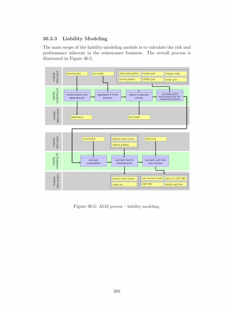
30.3.3 Liability Modeling
The main scope of the liability-modeling module is to calculate the risk andperformance inherent in the reinsurance business. The overall process isillustrated in Figure 30.5.
1
model baskets anddependencies
2
aggregate in forcebusiness
3
adjust to plannedvolume
4calculate gross
reinsurance loss incl.unearned business
mod
ule
data
inpu
tmod
ule
data
output
liability
mod
elling(I)
market cycle
GMDB cycle
inflation index
credit cycle
claims paid pattern
earning pattern
planning data loss model
dependency loss model
5
calculaterecoverables
6
calculate reservedevelopments
7
calculate cash flowand statistics
mod
ule
data
inpu
tbility
elling(II)
mod
ule
data
output
liamod
retrocession yield curve
new business results
UWY RBC
return on UWY RBC
liability cash flow
balance sheet reserve
reserve volatility
balance sheet reserve
credit risk
Figure 30.5: ALM process – liability modeling.
380

Data Entities
The following data entities occur in the liability modeling module:
Dataentity
Description
Loss model There are various types of loss models involved in theliability modeling process:
� Wherever available, the single loss models of eachcontract belonging to a modeling basket are im-ported from the pricing systems and aggregated.
� In some cases (e.g. for the nat cat perils or thejoint ventures) the loss models are aggregated by thecorresponding pricing teams and delivered in formof aggregate distributions.
� For certain types of life business, the loss modeledis delivered in form of cash flows.
All the non-life lines of business are eventually modeledas aggregate distributions by modeling basket (i.e. byLines of Business (LoB) and legal entity). The life modelsare implemented as a cash flow model (e.g. FinancialReinsurance business) or as a scenario based model (e.g.GMDB business).
Claims paidpattern,earningpattern
These data entities are taken from the reserve module.Please refer to the corresponding definitions. They areused to model the yearly loss cash flows as well as theportion of unearned business.
GMDBcycle
This entity is taken from the economic scenario generationmodule. Please refer to the corresponding definition. TheGMDB cycle is used to model the GMDB line of business.
Credit cycle This entity is taken from the economic scenario generationmodule. Please refer to the corresponding definition. Thecredit cycle is used to calculate the credit risk of liabilities(credit and surety business) and retrocessionnaires.
381

Retrocession Information on internal and external retrocession is usedto model the reinsurance recoverables. This data is pro-vided by the retrocession department.
BS reserve The initial reserve state is taken from the start balancesheet and split by line of business/legal entity in the re-serve modeling module. Within the ALM model, the re-serves of the future balance sheet are forecast.
Reservevolatility
This entity is taken from the reserve modeling module.Please refer to the corresponding definition. The reservevolatility is used to calculate the balance sheet forecast ofthe reserves.
Yield curve This entity is taken from the economic scenario generationmodule. Please refer to the corresponding definition. Theyield curve is used in order to discount results.
Credit risk On the liability side, the credit risk is currently calculatedfor the credit and surety business, as well as the credit riskof retrocessionnaires.
Newbusinessresults
Reinsurance results, such as loss ratios, combined ratios,premium volumes and cost ratios by line of business andlegal entity. Loss statistics are calculated both on a grossand on a retro basis.
UWY RBC The liability stand-alone risk based capital consumptionis calculated by line of business and legal entity. The di-versified risk-based capital is calculated in the aggregatedresults calculation module.
Return onUWY RBC
The return on the liability stand-alone RBC is calculatedin order to monitor the profitability of the new business.
Liabilitycash flow
The liability cash flow is one of the main outputs of theliability modeling module. They are used in the asset-modeling module in order to calculate the rollover of theasset portfolio.
382
Marketcycle,inflationindex
These data entities are taken from the economic scenariogeneration module. Please refer to the corresponding def-initions. Market cycle and inflation index will be used tomodel a stochastic dependency of claim sizes with the eco-nomic scenarios. This feature is not yet implemented inthe ALM model. This is why these entities are dashed inthe graph overview above.
Process Steps
The following process steps have to be carried out in liability modeling:
Processsteps
Description
Modelbasketsand depen-dencies
Depending on the plan, the granularity of model basketshas to be determined. The main decision criteria are togenerate homogeneous modeling units with a hierarchicalstructure. Furthermore, all business segments in the planhave to be modeled.Among all modeling baskets within a node of the hierar-chical tree, a copula dependency is modeled. This depen-dency structure is reviewed at the beginning of each ALMprocess together with underwriters and actuaries.
Aggregatein-forcebusiness
The basis for modeling the new business is the in-forcebusiness. In many cases, the individual loss distributionsby contract are loaded from the pricing system and aggre-gated by modeling basket. Whenever aggregate loss distri-butions are input (e.g. for nat cat perils), the aggregationstep is trivial.
Adjustto plannedvolume
The distributions obtained from the in-force business arescaled in order to reflect the planned volume. Proportionaland non-proportional business is scaled separately by legalentity and by LoB. Furthermore, a distinction is madebetween growth in number of contracts versus growth inshare (per-risk versus per-event scaling).
383

Calculategross rein-surancelossincludingunearnedbusiness
For the new non-life business, the losses are modeled byaggregate distributions and their dependencies. An anal-ogous computation is done for the unearned business ofprevious UW years. Losses are simulated from the cor-responding loss models, i.e. the loss distributions, theGMDB cycle etc. The payout patterns are taken fromthe reserve model and are used to calculate the loss cashflow per year. Inflation index and market cycle reflect acorrelation or anti-correlation of reinsurance losses withthe economic scenarios; this feature, however, is not yetimplemented. The credit cycle is used to calculate thecredit risk of the reinsurance business (credit and suretybusiness).
Calculaterecover-ables
Recoverables from internal and external retrocession arecalculated. This yields the net cash flows from the grosscash flows.
Calculatereserve de-velopments
The reserves are taken from the initial balance sheet. To-gether with the reserve volatilities, log normal distribu-tions are modeled to yield the reserve developments of thecalendar year. The reserve of the projected balance sheetis calculated.
Calculatecash flowandstatistics
The liability cash flows are calculated gross and net reflect-ing the new business loss, the retrocession recoverables, aswell as the reserve developments. Statistics are calculatedby line of business and legal entity based on the stand-alone liability risk.
Roles and Responsibilities
The roles and responsibilities involved in the liability-modeling process aredescribed in the following subsections.
Liability modeler: The liability modeler is responsible for the overallprocess of the liability module. The responsibilities are to
� Ensure overall correctness and consistency of all methods and imple-mentations used in the liability module
� Ensure overall consistency of data within the liability modeling module
384

� Coordinate the overall liability-modeling process
� Coordinate the overall sign-off procedures for the liability-modelingmodule
Planning coordinator: The planning coordinator has the responsi-bilities to
� Provide the planned volumes by line of business, legal entity, and typeof business (prop. vs. non-prop)
� Provide the planned loss ratios by line of business, legal entity, andtype of business (prop. vs. non-prop),
� Provide the planned cost ratios by line of business, legal entity, andtype of business (prop. vs. non-prop)
� Provide information on the growth assumptions (new business vs.growth of existing business)
� Assist in the refining of the granularity of planning data to modelingbaskets
� Provide a sign-off on the final planning data by modeling basket andlegal entity
� Help ensuring consistency between pricing and planning
� Participate in the sign-off of the ALM liability model
Pricing actuary: There are several pricing actuaries involved in theALM process, depending on the organizational structure of the company.Currently, separate pricing actuaries are responsible for the standard non-life business, the nat cat business, life business, special contracts (Lloyd’s,Global Aerospace Underwriting Managers (GAUM), Medical Defense Union(MDU)) etc. The responsibilities of the pricing actuary in the ALM processare to
� Timely deliver loss models on the corresponding business if not auto-matically available in the pricing systems
� Provide explanations on the loss models, especially also regarding theinteraction with loss models of the other business segments
� Participate in the sign-off of the ALM liability model
385

Unearned business modeler: The unearned business modeler hasthe responsibilities to
� Derive and implement the loss distributions of unearned business bymodeling basket and legal entity from the new business model basedon earning patterns
� Ensure correctness of the methods and implementations used to createthese loss models and ensure their consistency with the rest of the ALMmodel
� Participate in the sign-off of the ALM liability model
New business modeler: The new business modeler has the respon-sibilities to
� Create the modeling baskets according to the planned business
� Discuss and review the dependency tree with underwriters and pricingactuaries
� Refine the granularity of planning data if necessary
� Collect the loss models from the pricing system or from the corre-sponding pricing actuaries
� Generate the aggregated loss models by modeling basket and legalentity
� Model cost ratios per modeling basket and legal entity
� Coordinate the feedback with the planning coordinator and pricingactuaries for explanations regarding the loss models and consistencybetween planning and pricing
� Ensure correctness of the methods and implementations used to createthe loss models and ensure their consistency with the rest of the ALMmodel
� Achieve the sign-off on the gross underwriting year loss statistics
ESG manager: The responsibilities of the economic scenario modelerin the liability modeling module are to
� Timely deliver the economic scenarios for yield curves, market cycle,inflation index, GMDB cycle and credit cycle
� Provide explanations on the economic scenarios if required
386

Retrocession coordinator: The retrocession coordinator is the con-tact in the retrocession department for the ALM process. The responsibili-ties are to
� Provide up-to-date information on internal and external retrocession
� Provide explanations on the retrocession information as needed
� Participate in the sign-off of the net underwriting year loss statistics
Retrocession modeler The responsibilities of the retrocession mod-eler are to
� Model internal and external retrocession in the ALM model
� Ensure correctness of the retrocession methods and implementationsused in the ALM model
� Collect the up-to-date information on internal and external retroces-sion from the retrocession department
� Achieve the sign-off of the net underwriting-year loss statistics
Reserve modeler The responsibilities of the reserve modeler in theliability modeling module are to:
� Timely deliver balance sheet reserve states and calendar year reservevolatilities
� Provide a mapping of reserving lines of business to the new businessmodeling baskets
� Ensure consistency of the reserve model with the new business model
387
Sign-off procedures
Overall, the liability modeler is responsible that the data entities of theliability modeling module achieve the appropriate sign-off. Please see theAppendix for an overview of the sign-offs given in the ALM process. Withinthe liability-modeling module, sign-off has to be achieved for the followingdata entities:
Dataentity
Description
GrossUWYlossstatistics
The new business modeler is responsible to coordinate andachieve the sign-off of gross underwriting-year loss statistics.The sign-off is given by the planning coordinator and thepricing actuary. As there is an impact of the economic sce-narios on the gross underwriting-year loss statistics, the eco-nomic scenario modeler is also involved in the sign-off proce-dure.
NetUWYlossstatistics
The sign-off of net underwriting-year loss statistics is basedon a sign-off of the gross underwriting-year loss statistics.The retrocession modeler is responsible to achieve the sign-off from the planning coordinator and the retrocession co-ordinator.
388

30.3.4 Asset Modeling
The main purpose of the asset modeling module is to calculate the perfor-mance and risk inherent in the asset management. The asset portfolio isstylized, valuated, and rolled-over taking into account the cash flows on theliability side. The asset modeling module is illustrated in Figure 30.6.
1
model stylisedportfolio
2
model dvlpmt. ofasset portfolio
3
calculate assetperformance & risk
4
calculate assetsensitivity
mod
ule
data
inpu
tmod
ule
data
output
asset
mod
elling
strat. asset allocation
credit cycle
liability cash flow
external parameters
investment index
FX rates
asset portfolio yield curve
asset portfolio asset sensitivity
credit risk
risk based capital
asset performance
Figure 30.6: ALM process – asset modeling.
Data entities
The following data entities are involved in the asset-modeling module.
Dataentity
Description
Assetportfolio
The asset portfolio is the collection of assets held by thecompany. The initial asset portfolio is delivered by the as-set management department. The asset portfolio consists ofvarious asset classes such as government bonds, corporatebonds, equity, real estate, interest rate hedges etc. Withinthe asset-modeling module, it is stylized and rolled forwardaccording to the development of the economy and the lia-bility cash flows. The final asset portfolio is output fromthe module.
Yieldcurve
This data entity is taken from the economic scenario gener-ation module. Please refer to the corresponding definition.The yield curve is used for calculating present values of as-sets.
389
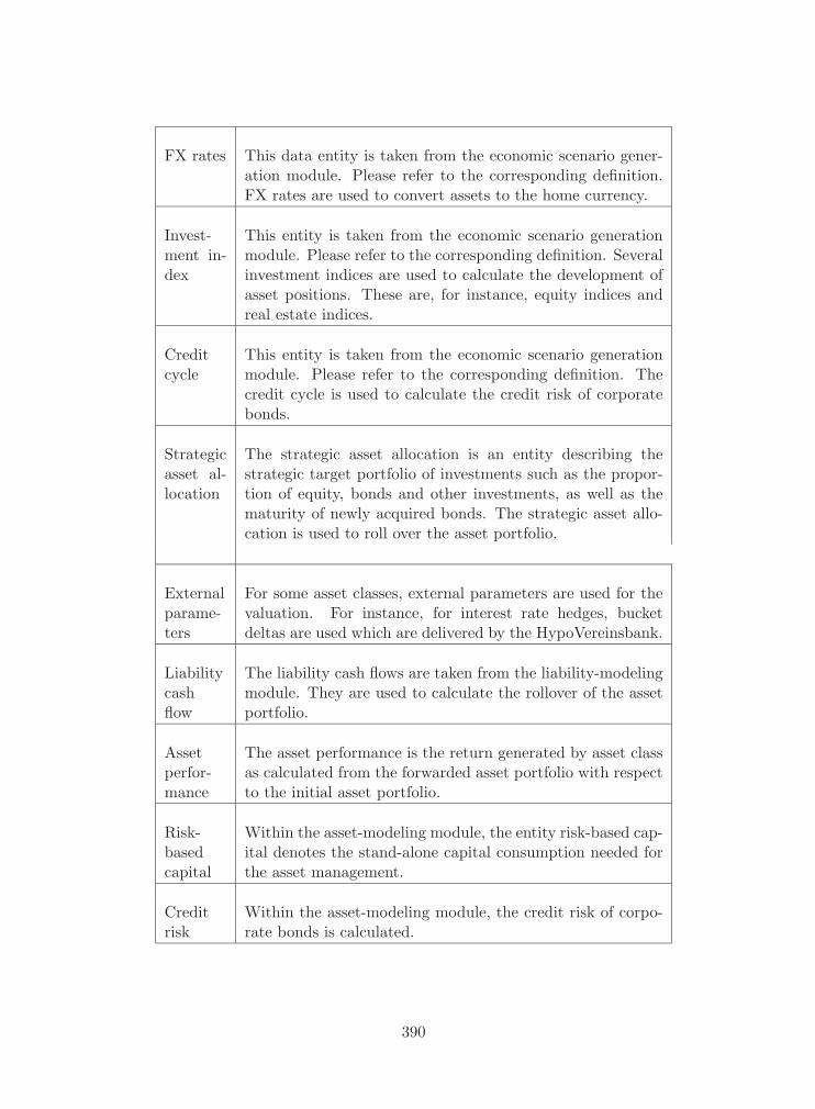
FX rates This data entity is taken from the economic scenario gener-ation module. Please refer to the corresponding definition.FX rates are used to convert assets to the home currency.
Invest-ment in-dex
This entity is taken from the economic scenario generationmodule. Please refer to the corresponding definition. Severalinvestment indices are used to calculate the development ofasset positions. These are, for instance, equity indices andreal estate indices.
Creditcycle
This entity is taken from the economic scenario generationmodule. Please refer to the corresponding definition. Thecredit cycle is used to calculate the credit risk of corporatebonds.
Strategicasset al-location
The strategic asset allocation is an entity describing thestrategic target portfolio of investments such as the propor-tion of equity, bonds and other investments, as well as thematurity of newly acquired bonds. The strategic asset allo-cation is used to roll over the asset portfolio.
Externalparame-ters
For some asset classes, external parameters are used for thevaluation. For instance, for interest rate hedges, bucketdeltas are used which are delivered by the HypoVereinsbank.
Liabilitycashflow
The liability cash flows are taken from the liability-modelingmodule. They are used to calculate the rollover of the assetportfolio.
Assetperfor-mance
The asset performance is the return generated by asset classas calculated from the forwarded asset portfolio with respectto the initial asset portfolio.
Risk-basedcapital
Within the asset-modeling module, the entity risk-based cap-ital denotes the stand-alone capital consumption needed forthe asset management.
Creditrisk
Within the asset-modeling module, the credit risk of corpo-rate bonds is calculated.
390
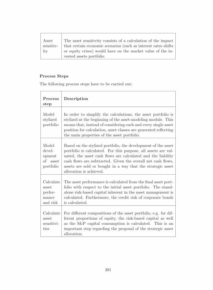
Assetsensitiv-ity
The asset sensitivity consists of a calculation of the impactthat certain economic scenarios (such as interest rates shiftsor equity crises) would have on the market value of the in-vested assets portfolio.
Process Steps
The following process steps have to be carried out:
Processstep
Description
Modelstylizedportfolio
In order to simplify the calculations, the asset portfolio isstylized at the beginning of the asset-modeling module. Thismeans that, instead of considering each and every single assetposition for calculation, asset classes are generated reflectingthe main properties of the asset portfolio.
Modeldevel-opmentof assetportfolio
Based on the stylized portfolio, the development of the assetportfolio is calculated. For this purpose, all assets are val-uated, the asset cash flows are calculated and the liabilitycash flows are subtracted. Given the overall net cash flows,assets are sold or bought in a way that the strategic assetallocation is achieved.
Calculateassetperfor-manceand risk
The asset performance is calculated from the final asset port-folio with respect to the initial asset portfolio. The stand-alone risk-based capital inherent in the asset management iscalculated. Furthermore, the credit risk of corporate bondsis calculated.
Calculateassetsensitivi-ties
For different compositions of the asset portfolio, e.g. for dif-ferent proportions of equity, the risk-based capital as wellas the S&P capital consumption is calculated. This is animportant step regarding the proposal of the strategic assetallocation.
391
Roles and Responsibilities
The roles and responsibilities are defined for the asset-modeling module asfollows:
Asset modeler: The asset modeler is the main role of the asset-modeling module. The responsibilities are to
� Collect the information needed on the current asset portfolio from theasset management coordinator
� Ensure correctness of the input data
� Ensure that all methods and implementations in the asset-modelingmodule are appropriate and correct
� Model the stylized portfolio
� Calculate the final asset portfolio, the asset performance, risk-basedcapital, the credit risk of corporate bonds, as well as the asset sensi-tivity
� Achieve a sign-off of the final results from the chief investment officer
Asset manager: The asset management coordinator is responsible to
� Timely deliver the information needed on the current asset portfolio
� Provide explanations on the asset portfolio as needed
� Participate in the sign-off of the final results
Chief Investment Officer (CIO):
� Provide the sign-off on performance target of the asset portfolio
Sign-off Procedures
A sign-off is needed for the asset performance. This sign-off is closely re-lated to the economic scenarios and is therefore to be coordinated with theeconomic scenario modeler. The asset performance is signed-off by the chiefinvestment officer. Please see the Appendix for an overview of the sign-offsgiven in the ALM process.
392
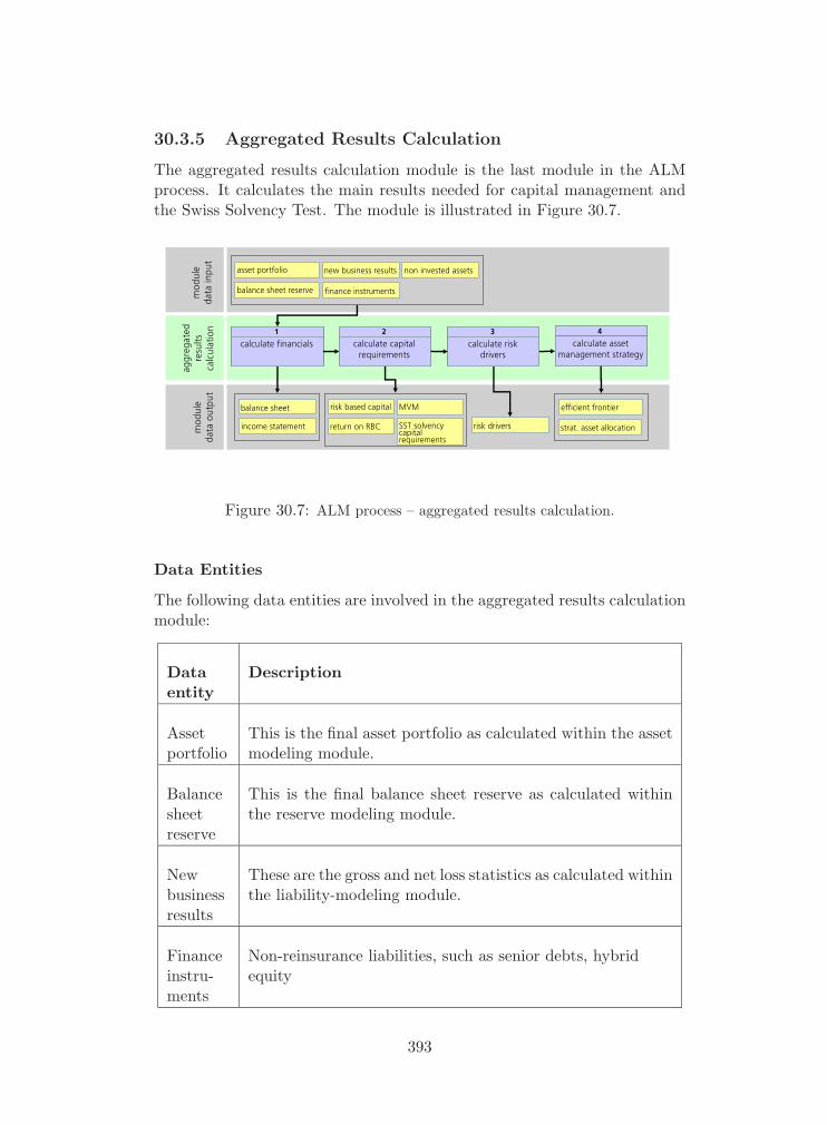
30.3.5 Aggregated Results Calculation
The aggregated results calculation module is the last module in the ALMprocess. It calculates the main results needed for capital management andthe Swiss Solvency Test. The module is illustrated in Figure 30.7.
1
calculate financials
balance sheet
income statement
2
calculate capitalrequirements
3
calculate riskdrivers
4
calculate assetmanagement strategy
asset portfolio
balance sheet reserve
new business results
efficient frontier
strat. asset allocation
efficient frontier
strat. asset allocation
mod
ule
data
inpu
tmod
ule
data
output
aggreg
ated
results
calculation
risk based capital
return on RBC risk drivers
finance instruments
non invested assets
MVM
SST solvencycapitalrequirements
Figure 30.7: ALM process – aggregated results calculation.
Data Entities
The following data entities are involved in the aggregated results calculationmodule:
Dataentity
Description
Assetportfolio
This is the final asset portfolio as calculated within the assetmodeling module.
Balancesheetreserve
This is the final balance sheet reserve as calculated withinthe reserve modeling module.
Newbusinessresults
These are the gross and net loss statistics as calculated withinthe liability-modeling module.
Financeinstru-ments
Non-reinsurance liabilities, such as senior debts, hybridequity
393

Non-investedassets
Non-invested assets, such as retro assets, funds held by rein-sured, deferred tax assets, goodwill.
Balancesheet
The main items of the nominal balance sheet are calculated.Furthermore, the Swiss Solvency Test and Solvency II requirecalculation of the main items of the economic balance sheet.
Incomestate-ment
The main items of the nominal income statement are calcu-lated. Furthermore, the Swiss Solvency Test and Solvency IIrequire calculation of the main items of the economic incomestatement.
Risk-basedcapital(RBC)
The overall diversified risk-based capital is calculated on acalendar year basis. Statistics are provided on details of thebusiness segmentation such as the net underwriting risk, thenet reserving risk and the asset risk. Furthermore, the diver-sity gain is calculated by comparing the stand-alone RBC tothe diversified RBC.
Returnon RBC
The return on RBC is calculated as a measure of the perfor-mance.
MVMmarketvaluemargin
As defined by FOPI, see SST white paper (FOPI [2004])
SSTsolvencycapitalrequire-ments
SST solvency capital requirements: As defined by FOPI, seeSST white paper (FOPI [2004])
Riskdrivers
The main risk drivers are calculated for both the assets andthe liabilities.
Efficientfrontier
Efficient frontiers are calculated by varying asset allocationsfor the portfolio rollover.
Strategicasset al-location
A new strategic asset allocation is derived from the efficientfrontier.
394

Process Steps
The following process steps have to be carried out:
Processstep
Description
Calculatefinancials
The nominal as well as the economic balance sheet and incomestatement are calculated by mapping the final asset portfo-lio, the final loss statistics, as well as the final balance sheetreserves to the corresponding positions of the balance sheetand the income statement.
CalculateSSTsolvencyrequire-ments
The calendar year risk based capital is calculated by calculat-ing the risk measure, i.e. the 1% shortfall, of the overall resultdistribution. The RBC is split to the various sub-segments,and the return on RBC is calculated. The MVM and the SSTsolvency capital requirements are calculated.
Calculaterisk drivers
The main contributions of single risk drivers to the calendaryear RBC are calculated and listed as the risk drivers.
Calculateasset man-agementstrategy
The ALM model is evaluated multiple times using differentallocations for the asset portfolio rollover. Each calculationyields a point for the efficient frontier. From the efficientfrontier, the strategic asset allocation is determined.
Roles and Responsibilities
We display the roles and responsibilities involved in aggregated results cal-culation:
Aggregated results calculator
� Ensure consistency and correctness of methods and implementationsused in the module
� Ensure consistency of the input data as collected from the other mod-ules
� Calculate the output data entities of the module
� Achieve sign-off from the ALM business owner
395

Financial controller
� Provide data and explanations on finance instruments and non-investedassets
ALM business owner
� Provide sign-off on aggregated results
ALM Committee
� Provide sign-off on projected balance sheet and income statement re-sults
� Provide sign-off on efficient frontier
� Provide sign-off on the ALM and SST Reports
Sign-off Procedures
As the results of the aggregated results calculation module are the mainresults of the ALM process, and as there are no modeling steps involved apartfrom the ones carried out in the previous modules and signed-off there, theoutput data entities of the aggregated results calculation module are signedoff by the ALM Committee directly.
As mentioned in the overview section, the results are assembled in tworeports: The ALM report and the SST report. The ALM Committee signsoff on both reports. Eventually, the SST report is submitted to the FOPI.Please see the Appendix for an overview of the sign-offs given in the ALMprocess.
396
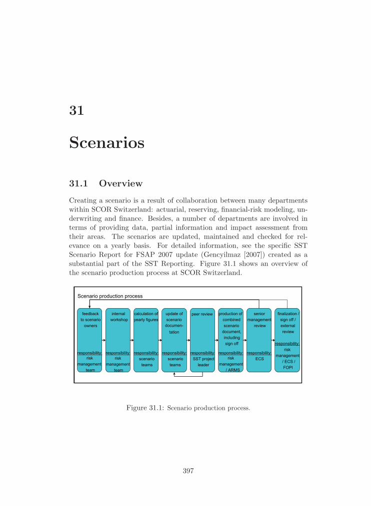
31
Scenarios
31.1 Overview
Creating a scenario is a result of collaboration between many departmentswithin SCOR Switzerland: actuarial, reserving, financial-risk modeling, un-derwriting and finance. Besides, a number of departments are involved interms of providing data, partial information and impact assessment fromtheir areas. The scenarios are updated, maintained and checked for rel-evance on a yearly basis. For detailed information, see the specific SSTScenario Report for FSAP 2007 update (Gencyilmaz [2007]) created as asubstantial part of the SST Reporting. Figure 31.1 shows an overview ofthe scenario production process at SCOR Switzerland.
feedback to scenario
owners
responsibility:risk
managementteam
internalworkshop
responsibility:risk
management team
calculation of yearly figures
responsibility:scenario
teams
update of scenario
documen-tation
responsibility:scenarioteams
peer review
responsibility:SST project
leader
production of combined scenario
document, includingsign off
responsibility:risk
management / ARMS
senior management
review
responsibility:ECS
Scenario production process
finalization / sign off / external review
responsibility:risk
management / ECS / FOPI
Figure 31.1: Scenario production process.
397

31.2 Process Steps
The following steps are taken during the scenario production process:
Process step Description
Feedback toscenarioowners
The yearly feedback by the FOPI is communicated by therisk management team to all scenario teams in separatemeetings.
Internalworkshop
In a workshop the specific teams define which scenariosare the largest threat to SCOR Switzerlands portfolio, re-spectively which scenarios need to be accomplished con-tinuously and which can be held back.
Calculation ofyearly figures
The data providers hand over the data for the scenarioproduction. For further details, see the specific scenariodocumentation.
Update ofscenariodocumentation
The scenario documentation is maintained and reviewedfor up-to-dateness. The major goal of this step is to focuson improvements in terms of transparency and ability toreplicate the analysis in the future.
Peer review Each scenario is peer-reviewed by SCOR Switzerland’srisk management team and the feedback is incorporatedinto the document.
Production ofcombinedscenariodocument
SCOR Switzerland’s risk management team writes a draftof the combined scenario document, including an ex-ecutive summary. The document is reviewed by theARMS (actuarial and risk management services) lead-ership group. It is also signed off for submission to seniormanagement.
Seniormanagementandexternalreview
The document is reviewed by the ECS.
398

Finalization ofthe combinedscenario docu-ment/ sign-off
ECS feedback is incorporated and the final document getssigned-off by ECS for delivery to FOPI.
31.3 Roles and Responsibilities
The following roles and responsibilities are defined for the scenario produc-tion process:
Role Description
SST processmanager
� Overall responsibility for the production of all sce-narios
� Perform peer review
� Manage flow of information to update scenariodocumentation
� Performing the role of the scenario documentationowner in collaboration with the risk managementteam
Scenarioteams
� Calculate and document respective scenarios
� Define, acquire and check all data needed for cal-culation
399
Risk man-agementteam
� Manage flow of feedback from internal senior man-agement and external review to the scenario own-ers
� Performing the role of the scenario documentationowner in collaboration with the SST project leader
ECS
� Challenge whether scenarios include all possiblelosses
� Challenge whether there are other more severe sce-narios
� Review the scenarios for delivery to FOPI
� Sign-off by CEO, CFO and COO
Scenariodocumenta-tion owner
� Main point of contact for FOPI regarding scenar-ios
� Define scenarios in cooperation with senior man-agement
Scenariodocumenta-tion editor
� Edit and structure the scenario document
� Communicate requirements to individual scenarioteams
� Ensure timely delivery of scenarios by scenarioteams
400

31.4 Sign-off Procedures
Sign-off (Table 31.1) is given by local CEO, CFO and COO for delivery toFOPI. In addition there is peer review and senior management review ofscenarios.
internal reviewseniormgmt.
ECS peerreview
methodologyparameters -Data -processesResults
Table 31.1: Scenario production process – sign-off matrix.
401

32
Appendix
32.1 Sign-off Matrix
32.1.1 Timeline of Project
SCOR Switzerland has set up the SST implementation project in February2006. All internal models for the ALM process have been reviewed, adjustedwhere needed and validated considering the guidelines provided by the FOPIfor the SST. The ALM process within SCOR Switzerland is considered in-dustry state-of-the-art over years (reference: Report from Oliver Wymann,2003). Based on this ALM process, with the necessary adjustments to befully SST compliant, SCOR Switzerland will create the yearly SST Reportfrom Q1/2008 onwards. Figure 32.1 shows SCOR Switzerland’s timeline toimplement the SST within its organization.
402

Kick off:Project
description and plan
Approval by GEC
Internal review of
model (complete
by end 2006)
Establish team,
confirm timelines, budget &
deliverables (by end
June 2006)
External validation of the Model
(complete by end 2007)
Perform Q3/07 ALM
exercise and create Draft SST Report
Model, system and process
documentation (complete by
end 2007)
Feb 22, 2006
Perform Q1/08 ALM
exercise and create first
SCOR Switzerland SST Report
April 1, 2008
Perform Q3/08 ALM
exercise and create Draft SST Report
Perform Q1/09 ALM
exercise and create second SCOR
Switzerland SST Report
Set up documen-
tationrepository
Finalize Model and Institutionalize Governance Framework
(complete by Oct. 2007)
Complete prototype of new model
(by Oct. 2006)
Figure 32.1: Timeline to implement the SST at SCOR Switzerland.
32.1.2 Project – Sign-off Matrix
To ensure consistency of model methodology, implementation, data and pro-cesses, SCOR Switzerland has developed a sign-off matrix for the SST im-plementation process (Table 32.1). As can be seen from the sign-off matrix,the documentation of all steps is subject not only to internal review but alsoto external review, especially, a full disclosure to the FOPI.
internal reviewpublic disclosuresenior mgmt. internal audit
external review FOPI
methodology - optionallyparameters - - optionallydata -implementation - - optionallyprocesses optionally
Table 32.1: SST project – sign-off matrix.
32.1.3 Project Roles and Responsibilities
Establishing an effective organization structure for a project is crucial to itssuccess. Every project has a need for management, direction, control andcommunication, so does the SST implementation process at SCOR Switzer-land. The following roles bring together the various interests, skills, man-agement and support:
403

Steeringcommit-tee:
The role of the steering committee is to confirm theproject objectives, provide guidance and direction to theproject and agree the project approach. The steeringcommittee approves deviations to plans and signs off onthe completion of project stages.
The steering committee commits the necessary resourcesto the project, arbitrates conflicts and assists in themanagement of issues as escalated by the project man-ager. The group is responsible for the acceptance of theproject’s risk management strategy and oversees the ex-ecution of that strategy.
Projectsponsor:
The project sponsor is the executive ultimately account-able for the project within SCOR Switzerland. He/sheensures that the project gives value for money and assuch owns and ensures the validity of the business case.
Businessowner:
Ensures that the end product is fit for its purpose andthat the solution will meet the user/business needs withinthe constraints of the business case. The business owneris responsible for provision of business resources and mustbe of sufficient authority to take decisions on project mat-ters. The business owner is ultimately responsible for thesign-off on the project’s products. The new organizationaids in the implementation of this model as a result ofglobal responsibilities.
Resourceprovider:
The resource providers are accountable for the qualityof the products delivered. They commit significant re-sources to the project and are of sufficient authority totake decisions on project matters. They deliver the re-sults desired by the business owner within the time andcost parameters of the business case.
SolvencyII liaison:
Ensures the alignment of SCOR Switzerland Cologne re-garding the preparatory activities for Solvency II in theEU with the SST project, capitalizing on synergies.
404

FOPI liai-son:
Takes the lead in FOPI liaison and is ultimately responsi-ble for ensuring that the regulatory requirements are metby the solutions proposed.
Projectmanager:
The project manager is responsible for the day-to-daymanagement of the project. Delivers the project withinthe agreed time, scope and cost. Due to the complexity,strong project management will be required.
Projectcore team:
The core team may be supplemented with additional re-sources and may change as a result of detailed planningand progressing work. The above team reflects the en-visaged goals and work during 2006 (Phase 1). The coreteam will be in charge of ensuring the timely delivery ofthe results. The team will naturally include the projectmanager.
32.1.4 Project Organizational Overview of Roles andResponsibilities
The above mentioned roles are organized in three different segments: steer-ing / structuring and validating / executing. This separation of segmentsis crucial to the success of the project as it strengthens internal audit andobjectiveness of results.
405

Steering
Stucturing& validating
Executing (develop, test,
document)
Function Body Responsible for
Sponsor
Steering committee
Business owner
Core team
Project management- Budget & reporting- Infrastructure, etc …
Liabilitymodel
Assetmodel
Credit risk model
Scenarios
L&H L&H L&H L&H
Integration
Life & health model specifics
Provide plan. + fin. data
ProvideIT tools
Model- / system - / Process documentation
Compliance
ResourcingDecisions
Coverage
Quality time line Costs
Figure 32.2: Organizational overview of roles and responsibilities.
406

VIII
SST Systems
407

Table of Contents
33 Summary 412
34 Introduction 413
34.1 Scope of the IT Systems Documentation . . . . . . . . . . . . 414
34.2 ALM Systems and ALM Process . . . . . . . . . . . . . . . . 415
35 Architecture of SST Relevant Systems 416
35.1 Software Development Process . . . . . . . . . . . . . . . . . 417
35.1.1 Software Development Life Cycle (SDLC) . . . . . . . 417
35.1.2 Application Change Management (ACM) . . . . . . . 418
35.2 Security . . . . . . . . . . . . . . . . . . . . . . . . . . . . . . 419
35.3 Revision Control . . . . . . . . . . . . . . . . . . . . . . . . . 420
36 Detailed Description of Systems 421
36.1 Language Definition . . . . . . . . . . . . . . . . . . . . . . . 421
36.2 Economic Scenario Generation . . . . . . . . . . . . . . . . . 422
36.2.1 Functional Overview . . . . . . . . . . . . . . . . . . . 422
36.2.2 System Overview . . . . . . . . . . . . . . . . . . . . . 423
36.2.3 Financial and Economic Database (FED) . . . . . . . 425
36.2.4 ESG Application . . . . . . . . . . . . . . . . . . . . . 426
36.2.5 Data Export . . . . . . . . . . . . . . . . . . . . . . . 428
36.3 Reserve Modeling . . . . . . . . . . . . . . . . . . . . . . . . . 429
36.3.1 Functional Overview . . . . . . . . . . . . . . . . . . . 429
36.3.2 Systems Overview . . . . . . . . . . . . . . . . . . . . 430
36.3.3 CORE . . . . . . . . . . . . . . . . . . . . . . . . . . . 431
36.3.4 ReCube . . . . . . . . . . . . . . . . . . . . . . . . . . 431
36.4 Modeling New and Unearned Business . . . . . . . . . . . . . 431
408

36.4.1 Functional Overview . . . . . . . . . . . . . . . . . . . 431
36.4.2 Systems Overview . . . . . . . . . . . . . . . . . . . . 433
36.4.3 Phobos . . . . . . . . . . . . . . . . . . . . . . . . . . 434
36.4.4 MARS . . . . . . . . . . . . . . . . . . . . . . . . . . . 435
36.4.5 Global Cat Data Platform . . . . . . . . . . . . . . . . 435
36.4.6 Planning and Business Projections: GPT . . . . . . . 436
36.4.7 Retrocession . . . . . . . . . . . . . . . . . . . . . . . 436
36.4.8 Life & Health Liabilities . . . . . . . . . . . . . . . . . 437
36.5 Assets . . . . . . . . . . . . . . . . . . . . . . . . . . . . . . . 438
36.5.1 Functional Overview . . . . . . . . . . . . . . . . . . . 438
36.5.2 Systems Overview . . . . . . . . . . . . . . . . . . . . 438
36.6 Risk Simulation . . . . . . . . . . . . . . . . . . . . . . . . . . 439
36.6.1 Functional Overview . . . . . . . . . . . . . . . . . . . 439
36.6.2 Systems Overview . . . . . . . . . . . . . . . . . . . . 440
36.7 Presentation of Results . . . . . . . . . . . . . . . . . . . . . . 441
37 Architecture of New Developments 442
37.1 Basic Architecture of Applications . . . . . . . . . . . . . . . 442
37.2 ALM Information Backbone . . . . . . . . . . . . . . . . . . . 443
37.3 Full Data Historization . . . . . . . . . . . . . . . . . . . . . . 443
37.4 Separating Data from Methods . . . . . . . . . . . . . . . . . 444
37.5 Design Principles . . . . . . . . . . . . . . . . . . . . . . . . . 444
37.5.1 Extensibility . . . . . . . . . . . . . . . . . . . . . . . 445
37.5.2 Maintainability . . . . . . . . . . . . . . . . . . . . . . 445
37.5.3 Testability . . . . . . . . . . . . . . . . . . . . . . . . . 445
37.5.4 Re-usability . . . . . . . . . . . . . . . . . . . . . . . . 446
37.6 Security . . . . . . . . . . . . . . . . . . . . . . . . . . . . . . 447
38 Appendix 448
409

List of Tables
36.1 Economic variables used for economic scenario generation. . . . . . 424
410

List of Figures
34.1 Overview of the ALM systems: functional needs. . . . . . . . . . . 413
36.1 ALM process – economic scenario generator . . . . . . . . . . . . 423
36.2 Economic Scenario Generation: Systems Overview. . . . . . . . . 425
36.3 The Financial Economic Database. . . . . . . . . . . . . . . . . . 426
36.4 The ESG – Igloo Interface. . . . . . . . . . . . . . . . . . . . . . 429
36.5 ALM process – reserve modeling . . . . . . . . . . . . . . . . . . 429
36.6 Data processing steps in reserve modeling. . . . . . . . . . . . . . 430
36.7 ALM process - liability modeling . . . . . . . . . . . . . . . . . . 432
36.8 Data processing steps in liability modeling. . . . . . . . . . . . . 434
36.9 The simulated performance of Life Business Liabilities depends onstochastic economic scenarios. . . . . . . . . . . . . . . . . . . . 437
36.10ALM process – asset modeling . . . . . . . . . . . . . . . . . . . 438
36.11The composition of the stylized asset portfolio is determined forsimulations in Igloo. . . . . . . . . . . . . . . . . . . . . . . . . 439
36.12Aggregate results calculation in Igloo. . . . . . . . . . . . . . . . 440
37.1 Basic architecture of applications. . . . . . . . . . . . . . . . . . 443
411
33
Summary
This Part of the documentation, based on SST Systems Documentation (Gutand Burgi [2008]), gives an overview of the software systems which are rele-vant for the calculation of SST results at SCOR Switzerland. The high levelarchitecture of existing systems and new developments is discussed. The ITsystems are mapped to the ALM process modules1.
1The documentation of the ALM and SST process together with the relevant processmodules is Skalsky and Burgi [2008] and is incorporated in Part VII of this documentation,see pp. 353.
412

34
Introduction
In the past decades, the importance of information technology in the finan-cial industry has increased significantly. With the growing data density grewthe need to develop appropriate techniques to extract information from thedata: The systems were interlinked, the system landscape was integrated,initially with a strong design focus on accounting and administration. Thecomplexity of handling data increased, especially in business areas whichwere not the main design focus for the IT system.
ALM Information Backbone
Data Entry
Data Generation
ESGData
enhancementRisk
simulation
Data Analysis
Data Reporting
Pricing Reserving Finance,Accounting
Planning AssetManagement
EconomicData
Figure 34.1: Overview of the ALM systems: functional needs.
Figure 34.1 shows schematically the functional needs of ALM systems.The ALM process is at the very end of the corporate process landscape:It takes information from many different departments. The main dataproviders are planning, asset management, pricing, reserving, accounting,
413

and Bloomberg. One of the purposes of ALM is to generate a holistic pic-ture of all cash flow relevant activities in the company. This step of matchingcode worlds, of resolving definition conflicts, of refining data to match therequired content definition and granularity, is an extremely demanding andtime-consuming step when calculating capital requirements of a reinsurancecompany.
It is not surprising that a large part of the SCOR Switzerland ALMsystem landscape consists of tools which were developed to handle theseinterfaces. Data have to be entered into the system. In some cases, datacan be transferred through automatic interfaces, in other cases data have tobe reformatted and entered manually into the system. This depends mostlyon the availability of appropriate systems on the counterparty end. Dataoften have to be enhanced (e.g. mapping codes or adjusting data to therequired granularity of data).
An important input to the internal model is a statistically balanced setof economic scenarios. SCOR Switzerland has developed a bootstrappingalgorithm to generate economic sceanrios. The ESG tool has been developedin house.
The means of computer simulation has proven to be efficient to imple-ment the models. The ability to efficiently implement complex calculationalgorithms is fundamental to building a sound and robust internal model.The risk simulation imports all the required data from the data entry andenhancement and the ESG parts and simulates the result-distribution of thecompany and all the other quantities relevant for the ALM and SST reports.
Eventually, the quantities generated in the risk simulation have to beanalyzed and formatted for use in the ALM and SST reports.
34.1 Scope of the IT Systems Documentation
The system landscape involved in the calculation of the ALM and SSTreports is rich. The ownerships of the interfacing systems reside in the cor-responding departments. The ownership of ALM specific systems resides inthe Financial Modeling department. For a detailed overview of ownerships,refer to Appendix (p. 448).
Since a large part of the data generated in the company are cash flowrelevant in one or the other way, most of the systems used in the companyare somehow involved in the ALM process. There is a core of ALM systemswith the risk simulation part in its centre and the other modules around itas described above. This documentation focuses mainly on the ALM specificsystems. Furthermore, it gives an outline of the interfacing systems. Thefurther away a system is from the core risk simulation, the less it will bedescribed in this documentation.
414

34.2 ALM Systems and ALM Process
A sound integrated management should consist of both, a solid methodologyand calculation process, and a robust ALM process. The main purposes ofthe ALM system landscape are to:
� Provide tools and methods to retrieve and refine input data
� Calibrate the models used in the ALM methodology
� Calculate all results necessary for the ALM and SST reports
� Support the ALM process
In this sense, the SST Systems Documentation is strongly interlinkedwith the SST methodology1 and the SST process landscape2. The modulesof the SST Process Landscape were designed to give a functional overview ofthe SST Process. In this document, the implementation in the ALM systemlandscape will be shown. This is a different perspective, and the charts willtherefore not be fully congruent. The link between the ALM systems andthe functional modules described in the ALM Process Landscape will bedescribed in detail.
1See parts I, II, III, IV, V, VI of this document.2Swiss Solvency Test (SST) at SCOR Switzerland: Process Landscape, Skalsky and
Burgi [2008], incorporated into this document as Part VII.
415

35
Architecture of SSTRelevant Systems
This chapter is divided in two major sections: one section describing thearchitecture of the existing systems and the other section highlighting thearchitectural principles used for new developments. The Economic ScenarioGenerator (ESG) has already been built along these principles. A projectis in preparation to implement these principles for all ALM specific compo-nents.
A vast variety of technologies is involved in the calculation of the ALMand SST reports, especially due to the high number of systems involved.The core risk simulation is implemented in Igloo, a generic DFA softwaredeveloped by EMB1.
The majority of the system landscape of former Converium relevant tothe SST was built in the .NET framework with Microsoft SQL databases.The new ESG has also been built in this technology. The SCOR systemsconsist mostly of Java and PowerBuilder applications with Sybase databases.The decisions on the future technologies to be used are pending at the timeof writing this documentation.
Most of the data input to the ALM model are usually exchanged inExcel or text file format. Exceptions: ESG data is read from the MS SQLdatabase directly into Igloo; the reserving data is transferred from MS SQLvia an OLAP layer to Excel. The data enhancement steps (mapping of codes,refining data to match the granularity needed, etc.) are usually implementedin Excel. Final inputs to the risk simulation in Igloo are stored in Excel ortext format and read via Igloo links into the risk simulation. Simulationoutputs are stored in Excel or text file format.
1http://www.emb.co.uk/
416

35.1 Software Development Process
35.1.1 Software Development Life Cycle (SDLC)
The Purpose of SDLC
The Software Development Life Cycle (SDLC) guidelines define the prin-ciples to ensure delivery or acquisition of software according to businessneeds, with business involvement and testing, using standards and methodsand providing appropriate documentation. The result will enable SCORSwitzerland to make proper use of the application and the technologicalsolution.
Process ownership
The main responsibility lies with the Head of IT Development at SCORSwitzerland who is the process owner and thus responsible for designing,implementing, changing, documenting and executing the process.
The processes covered by SDLC
The SDLC covers six processes:
1. It is ensured that the business side is appropriately involved in thedesign of applications, selection of packaged software.
2. It is ensured that an adequate development process is in place. Theprocess covers security, availability, and processing integrity aspects.
3. When new systems are implemented or existing systems are modified,controls are added, modified or redesigned to ensure that applicablecontrol objectives are achieved (including change management).
4. Controls exist to ensure there is adequate testing for the developmentor acquisition of systems and applications. Testing is signed off byboth the business side and IT.
5. Controls are in place to ensure that an appropriate system, user, andcontrol documentation is developed for new systems and applications,as well as for modifications of existing systems and applications.
6. Controls are in place to ensure that users are trained on new systems/applications used during financial reporting processes in accordancewith an appropriately defined training plan.
417

35.1.2 Application Change Management (ACM)
The Purpose of ACM
The Application Change Management (ACM) process is a business-drivenand cost efficient method of handling changes to SCOR Switzerland’s appli-cations. It ensures minimum negative impact and risks for SCOR Switzer-land’s business by requiring planning and initial impact analysis of all changerequested. Changes cannot be built or implemented outside the ACM pro-cess. The ACM process will increase substantially the quality of serviceSCOR IT delivers to the business side.
Process ownership
The ACM process is owned by the Head of IT Operations department.
Process Objectives
Business side objectives for the ACM process are:
� Ensure the business side is involved in the process of specifying, au-thorizing and setting priorities.
� Ensure that the Sarbanes-Oxley control environment for business con-trols are maintained.
� Ensure delivered solution meets requirements and specifications ofchange request.
� Ensure that the change has no negative impact on business.
� Ensure coordination within the business community.
� Ensure that the correct sign-offs are collected for changes.
� Ensure all audit and compliance requirements are met.
� Ensure efficient, prompt and documented handling of all changes.
Functional objectives for the ACM process are:
� Ensure Sarbanes-Oxley IT general controls have been performed.
� Minimize impact of changes to production environments.
� Ensure a clear segregation between development and production envi-ronments.
� Ensure change has no negative impact on IT Service Delivery.
� Ensure IT service quality is maintained as agreed.
418

� Ensure the use of standardized methods and procedures.
� Ensure configuration data and documentation are maintained.
� Ensure the IT Security of systems and applications is maintained.
� Save Cost by distinguishing changes by impact and priority.
� Save Cost by specifying solutions to problems before any developmentor implementation work is done.
Process Scope
The scope of the ACM process includes all software referenced in the scopesection of the policy for Configuration Management. Basically the scopeincludes all changes to financially relevant application software developedin-house or acquired for specific use within SCOR Switzerland. Also systemsoftware supporting to these applications are in scope.
The scope includes the Test/QA and Production environments and thefollowing application component changes:
� Program code
� Data structures
� Back-end data corrections
� Configuration files and Automated Jobs/Agents/Tasks
� Documentation and procedures associated with running, supportingand maintaining the application
The customizing of third part software is out of scope.
35.2 Security
The .NET / MS SQL systems are secured by role-based access management(RBAM). The RBAM is maintained according to the corporate guidelinesand can be found in the corresponding documentation.
All Excel and text files as well as the Igloo model are stored on NFS driveswith Windows access management. Access to the spread sheets, text filesand the Igloo model is restricted to the members of the Financial Modelingdepartment and single interfacing roles.
419

35.3 Revision Control
The key to gaining overview and transparency of data, methods and doc-umentation is a sound versioning and historization concept. All data en-tities, methods and documents underlie a clear release concept. Releasesare documented and labelled. Changes are documented. In order to ensurereproducibility and auditability of data, a clear historization concept hasbeen elaborated and implemented.
For all the systems which are maintained by the IT department, i.e.all the .NET / MS SQL systems, the revision control system used is IBMClear Case. For all the Excel and text files, as well as the Igloo model,the versioning system used is Microsoft Visual SourceSafe. All featuresfor check-in, check-out, roll-back are readily provided by the correspondingrevision control systems. Changes can be documented at the point of check-in, releases can be labelled.
420
36
Detailed Description ofSystems
This part of the SST Systems Documentation is strongly interlinked withthe SST Process Landscape (which is Part VII in this document, see pp.353). Whereas the functional modules described in the latter document aredesigned to reflect the content in its context, the present documentation aimsat describing the systems in their context. This leads to a slightly differentstructure; however, the link to the functional modules is given explicitly inall sections.
36.1 Language Definition
Throughout the next sections of this document the IT systems as well as therelevant data processing steps will be graphically displayed. The graphicsserve to illustrate the tools used and the data flows as specified in the text.Unidirectional or bidirectional arrows indicate the flow of data between ITsystems. Due to the complexity of the data processing steps, spread sheetcalculations are often involved. In order to differentiate between systemsor other data processing entities, database storages, data files and doc-uments, numerical operations, and manual input, we introduce the basicshapes shown in the following table.
421
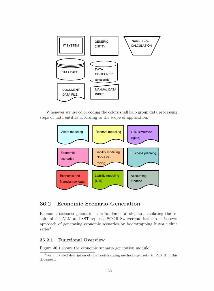
IT SYSTEM
DATA BASE
DOCUMENT,DATA FILE
MANUAL DATA INPUT
NUMERICALCALCULATION
GENERICENTITY
DATA CONTAINER
(unspecific)
Whenever we use color coding the colors shall help group data processingsteps or data entities according to the scope of application.
Accounting, Finance
Asset modeling
Liability modeling (Life)
Economic
scenarios
Reserve modeling
Liability modeling (Non- Life),
Pricing
Business planning
Risk simulation
(Igloo)
Economic and
financial raw data
36.2 Economic Scenario Generation
Economic scenario generation is a fundamental step to calculating the re-sults of the ALM and SST reports. SCOR Switzerland has chosen its ownapproach of generating economic scenarios by bootstrapping historic timeseries1.
36.2.1 Functional Overview
Figure 36.1 shows the economic scenario generation module.1For a detailed description of this bootstrapping methodology, refer to Part II in this
document.
422
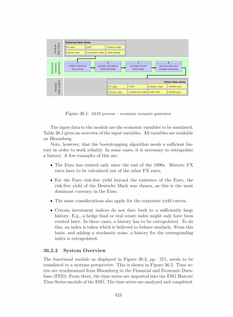
1
collect historicaltime series
2
analyse and adjusthistorical data
3
simulate futuretime series
4
post process andanalyse scenarios
1
collect historicaltime series
2
analyse and adjusthistorical data
3
simulate futuretime series
4
post process andanalyse scenarios
1
collect historicaltime series
2
analyse and adjusthistorical data
3
simulate futuretime series
4
post process andanalyse scenarios
FX rates
interest rates
GDP
investment index
inflation index
credit spread
historical time series
econ
omic
scen
ario
gene
ratio
n
FX rates
investment index
GDP
credit cycle
inflation index
GMDB cycle
future time series
mod
ule
data
inpu
tmod
ule
data
output
interest rates
market cycle
Figure 36.1: ALM process – economic scenario generator
The input data to the module are the economic variables to be simulated.Table 36.1 gives an overview of the input variables. All variables are availableon Bloomberg.
Note, however, that the bootstrapping algorithm needs a sufficient his-tory in order to work reliably. In some cases, it is necessary to extrapolatea history. A few examples of this are:
� The Euro has existed only since the end of the 1990s. Historic FXrates have to be calculated out of the other FX rates.
� For the Euro risk-free yield beyond the existence of the Euro, therisk-free yield of the Deutsche Mark was chosen, as this is the mostdominant currency in the Euro.
� The same considerations also apply for the corporate yield curves.
� Certain investment indices do not date back to a sufficiently largehistory. E.g., a hedge fund or real estate index might only have beencreated later. In these cases, a history has to be extrapolated. To dothis, an index is taken which is believed to behave similarly. From thisbasis, and adding a stochastic noise, a history for the correspondingindex is extrapolated.
36.2.2 System Overview
The functional module as displayed in Figure 30.3, pp. 371, needs to betranslated to a systems perspective. This is shown in Figure 36.2. Time se-ries are synchronized from Bloomberg to the Financial and Economic Data-base (FED). From there, the time series are imported into the ESG HistoricTime Series module of the ESG. The time series are analyzed and completed.
423

Entity Time series used
Risk-free yield Government bonds are not quite risk-free – there isstill a small credit risk of the corresponding coun-try priced in. Bloomberg has defined a set of fair-value risk-free yield curves which are calculated outof several liquid market instruments for each cur-rency. This set is taken as input for the risk-freeinterest rates.
Inflation Index The consumer price index (CPI) of the correspondingcurrency zone. For the Euro zone, an overall CPI isused. All CPIs are available in Bloomberg.
GDP The real GDP, i.e. the GDP net of inflation, isneeded. In Bloomberg, there is a mixture of nominaland real GDPs available. Wherever the real GDP isavailable, it is used as input. Otherwise, the nomi-nal GDP is imported and converted to a real GDPwithin the ESG Historic Time Series module (seePart II, pp. 193).
FX Rates The FX spot rates are chosen at the time of eachsimulation interval (i.e. end of a quarter or month).
Investment Index The investment indices matching the asset portfolioare chosen for simulation. These are the gross equityindices (MSCI daily), and for some currencies hedgefund or real estate indices.
Credit Spread Corporate yields are imported for a number of rat-ings (currently for A and BBB). From the corporateyields and the risk-free yields, the credit spreads arecalculated.
Table 36.1: Economic variables used for economic scenario generation.
424

ALM Information Backbone
FED
Non- -Bloombergtime series
Economicraw data
Enhancedtime series
EconomicScenarios
Bloomberg
Manual Input
Analysis, inter-
and extrapolation, statistical tests
ESG Datapost-
Igloo Import
Igloo interface
Reporting
Simulationprocessing
Figure 36.2: Economic Scenario Generation: Systems Overview.
The ESG Simulation module provides the bootstrapping algorithm, whichresults in the Economic Scenarios. From there, the data can be exported inthe Igloo Interface and then to Igloo. For ALM, there is no manual inputof time series required. This facility is only provided for other consumers ofeconomic scenarios.
36.2.3 Financial and Economic Database (FED)
The Financial and Economic Database (FED) is the central data provider oftime series. It is an in-house development. FED is implemented in MicrosoftSQL Server and .NET. The main dataprovider of FED is Bloomberg. Allsubscribed time series are updated nightly.
The scope of FED is to be an encapsulation layer between data providerssuch as Bloomberg and the company internal systems. This encapsulationlayer has the advantage that several data sources, usually with different codeworlds (e.g. their tickers) and database schemas, can be merged into onecommon data source, from where it can be served to the other applications.This situation is shown in Figure 36.3.
FED also has a user interface which allows to retrieve financial andeconomic data through a web browser or exported to an Excel sheet. FEDis owned by the Financial and Risk Modeling department and maintainedby IT Development.
The Economic Scenario Generator (ESG) is one of the main consumersof FED data. The data are imported directly from the FED database tothe ESG Historic Time Series module. There, they can be adjusted andcompleted for simulation purposes.
425

FED
User
Bloomberg Other sources
Application
decoupling
External Data
Source
Company
Business
Figure 36.3: The Financial Economic Database.
36.2.4 ESG Application
The ESG application consists of two distinct modules: the ESG HistoricTime Series, and the ESG Simulation modules as described in the nextsubsections. The ESG application is developed in the .NET framework withan MS SQL database.
The ESG application is owned by the Financial and Risk Modeling de-partment and maintained by IT Development.
ESG Historic Time Series
The ESG Historic Time Series module has the purpose to collect all timeseries required for simulation from FED. There is the concept of an ESGTicker, which contains the basic definition of a time series, such as the
� Code to be used in Igloo
� Type of ticker (GDP, CPI, equity etc.)
� Value definition (gross, price, dividend, total return)
� Inflation correction (nominal, real)
� Link to the FED source
The management of the ESG Tickers is enabled in the ESG applica-tion. The role of the ESG Ticker Manager is responsible to administer theESG Tickers such that they relate to the desired data source and to thecorresponding part in the Igloo model.
The role of the ESG Modeler is responsible to assemble the time serieshistory. Once the desired ESG Tickers are chosen for the ALM model, the
426

data can be automatically imported from FED. Note that, typically, theESG Historic Time Series module is updated by copying a previous one andby importing the most recent FED data. The ESG application supports thisuse case strongly by providing a color coding for which values correspondto the FED and which ones not, and by enabling a partial update of figuresfor a selection of individual items.
The ESG Historic Time Series module also provides facilities for inter-and extrapolating time series (vertically in time) and yield curves (hori-zontally in maturity). The vertical inter- and extrapolation is needed if thesimulated time series are not up-to-date, i.e. if a time series such as the GDPhas a certain delay of being reported. The horizontal inter- and extrapola-tion of yield curves is needed if maturities other then the ones supported byBloomberg are to be simulated.
Since it is difficult to validate a large amount of data, the ESG HistoricTime Series module also contains statistical tests which highlight deviationsof time series by more than the expected deviation. This feature allows toget a quick overview of suspicious values which have to be checked withinBloomberg. This would, for instance, be the case if an index was re-based.The application would highlight the place of re-basing, and the user couldmanually convert the index to one base.
For all deviations from the FED values, comments must be added to thededicated section. Once the time series history is completed and validated,the ESG Historic Time Series module is locked by the ESG Modeler. Lockingwill disable the update of the module. This is the procedure how a version ofthe data is administered. In order to create a new version, the ESG HistoricTime Series module can be copied, modified and locked.
ESG Simulation
The ESG Simulation module has the purpose to assemble the set of timeseries to be simulated, to select the simulation parameters, and to run thesimulation.
A selection of time series is necessary, as there is not a one-to-one cor-respondence between historic time series and simulated ones: For instancethe corporate yield curves are evaluated, together with the risk free yields,to the credit level, which is output from the simulation.
There are only few simulation parameters exposed on the user interface.The main ones are:
� The time interval denoting the historic period to be used for boot-strapping
� The time interval to be simulated
� The number of scenarios to be simulated
427

For investment indices, there is also an option to enter expert opinions:The main purpose of the ESG is not to calculate accurate forecasts but tocalculate an accurate spread around the forecasts. As the expert opinions arebased on a broader range of observations than pure stochastic bootstrappingfrom the history, they are to be preferred. It is thus possible to use (astochastic variant of) the expert opinions to adjust the expected net return.
All other parameters, i.e. the parameters underlying the economic mod-els, are hidden from the user. These parameters are the result of calibrationcalculations. Typically, they are only modified when the analysis of histor-ical data is updated or enhanced. This is a lengthy procedure which can,for instance, be done in the framework of a master’s thesis. When adjustingthe low-level parameters, and after extensive testing, the application wouldbe re-deployed with the new models.
A post-processing step allows for a further set of operations:
� The scenarios can be stochastically interpolated to other time intervals(e.g. from quarters to months). This is usually not needed in the ALMcontext.
� The scenario set can be concentrated, i.e. the number of scenarioscan be reduced. This is done along an extremeness metrics, which de-fines extreme scenarios. The most extreme scenarios are all kept. Thenumber of remaining (‘normal’) scenarios is reduced along the metrics,increasing the weights of the normal scenarios correspondingly. Sce-nario Concentration makes sense if the data transfer (e.g. import toIgloo) does not perform well enough.
� Time series can be scaled to a target over a given simulation interval.Studies show that, over a long time horizon such as 10 years, thereturn of an investment index is less volatile than the bootstrappingalgorithm would predict. Therefore, it is possible to scale scenarios toyield a certain long-term return. This feature is used for the scenariossubmitted to the life department, which cover a time horizon of severaldecades.
Another feature of the ESG Simulation module is that it can produceforecast tables over a specified forecast horizon. This forecast table is anintegral part of the ALM report.
Once the ESG Simulation is completed and appropriately commented,it is locked by the ESG Modeler. Only if a simulation is locked, it can beexported to Igloo.
36.2.5 Data Export
Within the ALM process, there are two main consumers of the economicscenarios: The actuarial life department who model the GMDB and financial
428

reinsurance life business using these scenarios, and the main risk simulationin Igloo. For transferring the data to the life department, they are exportedto an Access data base on an NFS drive.
For exporting the data to the main risk simulation in Igloo, the data aretransferred to the Igloo interface (Figure 36.4). Only locked simulation canbe exposed to Igloo. In Igloo, the economic scenarios can be read from theMS SQL Server, and are parsed to a proprietary Igloo file format.
ESG
Risk simulation (Igloo)ESG- Igloo
Interface
Figure 36.4: The ESG – Igloo Interface.
36.3 Reserve Modeling
The purpose of reserve modeling2 is to calculate the reserve volatilities aswell as to calculate the incurred (reported), paid and earnings patterns byline of business and by legal entity. Furthermore, the reserve duration andthe reserve run-off are calculated for inclusion in the ALM Report.
36.3.1 Functional Overview
Figure 36.5 shows the functional overview of the reserve modeling module.
1
calculate patterns
claims paid pattern
premium pattern
earning pattern
2
calculate balancesheet reserving
3
calculate reservevolatilities
4
calculate durationand statistics
incurred Triangle
paid triangle
case res. triangle
premium triangles
incurred Triangle
paid triangle
case res. triangle
premium triangles
BS reserve
reserve volatility reserve duration
reserve runoff
reserve duration
reserve runoff
yield curve
claims paid pattern
yield curve
claims paid pattern
mod
ule
data
inpu
tmod
ule
data
output
reserving
mod
ule
BS reserve
Figure 36.5: ALM process – reserve modeling
2The detailed aspects of the reserve model are considered in Part I of this documenta-tion.
429
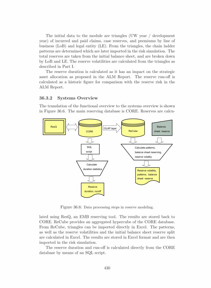
The initial data to the module are triangles (UW year / developmentyear) of incurred and paid claims, case reserves, and premiums by line ofbusiness (LoB) and legal entity (LE). From the triangles, the chain ladderpatterns are determined which are later imported in the risk simulation. Thetotal reserves are taken from the initial balance sheet, and are broken downby LoB and LE. The reserve volatilities are calculated from the triangles asdescribed in Part I.
The reserve duration is calculated as it has an impact on the strategicasset allocation as proposed in the ALM Report. The reserve run-off iscalculated as a historic figure for comparison with the reserve risk in theALM Report.
36.3.2 Systems Overview
The translation of the functional overview to the systems overview is shownin Figure 36.6. The main reserving database is CORE. Reserves are calcu-
Reserve
duration, runoff
ResQ OLAP layer
SQL
script
CORE ReCube
Calculate patterns,
balance sheet reserving,
reserve volatiliy
Reserve volatility,patterns, balance sheet reserve
Balance
sheet reserve
Calculate
duration statistics
Figure 36.6: Data processing steps in reserve modeling.
lated using ResQ, an EMB reserving tool. The results are stored back toCORE. ReCube provides an aggregated hypercube of the CORE database.From ReCube, triangles can be imported directly in Excel. The patterns,as well as the reserve volatilities and the initial balance sheet reserve splitare calculated in Excel. The results are stored in Excel format and are thenimported in the risk simulation.
The reserve duration and run-off is calculated directly from the COREdatabase by means of an SQL script.
430

36.3.3 CORE
CORE – Converium Reserving Estimator – is a reserve analysis tool anddatabase developed in-house. The analysis part of the application has beenreplaced by ResQ in 2007. The CORE database continues to exist as thedata provider to ResQ and main storage of all reserving data and for book-ings and accruals. The CORE database is implemented in Microsoft SQLServer, the front end is in PowerBuilder.
The application and data owner is the Reserving team (Actuarial – Non-Life). CORE is maintained by IT Developemnt.
36.3.4 ReCube
ReCube was internally developed by the company as a reporting tool to an-alyze reserving data and to produce reserve triangles. ReCube is a hypercubeon CORE (OLAP layer). Triangles can be imported directly from ReCubein Excel.
The applications and data owner is within the Financial Planning &Analysis team. ReCube is maintained by IT Development.
36.4 Modeling New and Unearned Business
Next to the reserving risk, the risk inherent in the new business3 is thesecond major part of the insurance risk . Currently, life and non-life businessis completely separated systemwise. Since SCOR Switzerland is mainlywriting non-life business, its system landscape is richer on the non-life partthan on the life part.
36.4.1 Functional Overview
Figure 36.7 shows the functional overview for modeling new and unearnedbusiness.
The planning data is analyzed carefully and based on it, and based on theexisting business, the modeling baskets are created. A dependency structurebetween the baskets is defined. The basket structure and dependency treeare hierarchical.
Loss models are imported from the pricing systems. This can either bedone by contract, upon which the contracts would be aggregated using thedependency within the basket. In some cases, the contracts are aggregated ina different manner; for nat cat perils, aggregate distributions are calculatedusing an event-set based approach. Large contracts are modeled in separatebaskets with the aggregate distributions entered directly into Phobos. Forlife business, there is a separate process in place. Generally, the loss scenarios
3The detailed aspects of the new business model are considered in Part I.
431
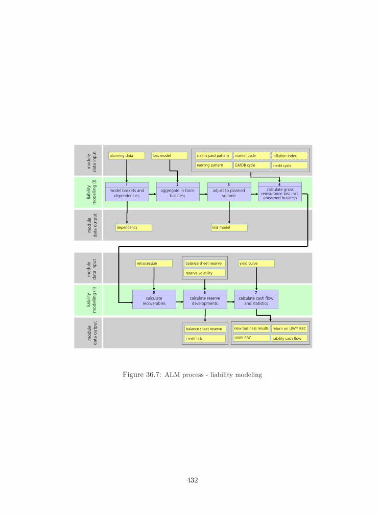
1
model baskets anddependencies
2
aggregate in forcebusiness
3
adjust to plannedvolume
4calculate gross
reinsurance loss incl.unearned business
mod
ule
data
inpu
tmod
ule
data
output
liability
mod
elling(I)
market cycle
GMDB cycle
inflation index
credit cycle
claims paid pattern
earning pattern
planning data loss model
dependency loss model
5
calculaterecoverables
6
calculate reservedevelopments
7
calculate cash flowand statistics
mod
ule
data
inpu
tbility
elling(II)
mod
ule
data
output
liamod
retrocession yield curve
new business results
UWY RBC
return on UWY RBC
liability cash flow
balance sheet reserve
reserve volatility
balance sheet reserve
credit risk
Figure 36.7: ALM process - liability modeling
432

depend on the economic scenarios as delivered by the ESG. Therefore, theactual loss distributions are generated only during the risk simulation. Theyare merged at this stage to the basket structure according to the dependencytree.
For the majority of the in-force business, loss models are available frompricing. However, the plan includes also business which is not yet writtenor which has not been priced. The assumption is taken that the non-pricedbusiness will behave similarly as the priced part of the portfolio. Therefore,the loss models as obtained from pricing are scaled to match the plannedvolume.
The underwriting-year statistics of the new business on a stand-alone ba-sis (i.e. disregarding developments in reserves, assets etc.) can be generatedat this stage. It is an important consolidation step to compare the plannedvolumes, loss ratios, profits and stand-alone RBC required in their aggre-gated form among the departments (pricing, nat cat and planning). Thishelps to enhance the overall quality of data in the company significantly.
The underwriting-year-based loss models are then processed with thepayment-and-earnings-patterns in order to yield the gross cash flow modelsfor new and unearned business. Information on the retrocession covers isprovided by the retrocession department. The loss models are imported inthe risk simulation, together with the data from the reserve modeling andthe information on the retrocession covers. In the risk simulation, the modelsare evaluated in conjunction to yield the net liability cash flow model.
36.4.2 Systems Overview
The translation of the functional overview as given above to the non-lifesystems overview is shown in Figure 36.8.
The Global Planning Tool (GPT) is used to plan the business by con-tract. From GPT, an Excel Pivot table is extracted, which is the entrypoint in the ALM model. The Pivot table is analyzed, the modeling bas-ket structure is prepared by segmenting the data further. Eventually, theplanned premiums and losses as well as the planned costs are available foreach modeling basket.
The basket structure is entered in Phobos, the main aggregation engine.The dependencies are added to the basket structure. Phobos has a directinterface to MARS, the main non-life treaty pricing system. The MARStreaties can be assigned to the modeling baskets, and the NPV, premium,loss, cost distributions and also development patterns can be imported au-tomatically for aggregation. Other data sources can be added by copyingand pasting aggregate discrete distributions.
Once the reference volumes of the in-force part of the business is known,separate scaling factors for growth in the number of contracts and growthin share can be entered in Phobos. These scaling factors are calculated in a
433
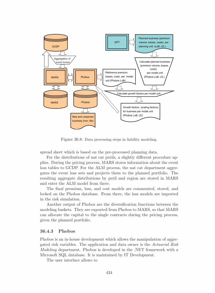
MARS Phobos
Phobos
New and unearned business (non- life)
GPT
MARS
Reference premium,losses, costs per modelunit (Phobos LoB)
Calculate growth factors per model unit
Growth factors (scaling factors)for business per model unit(Phobos LoB, LE)
Planned business (premium volume, losses, costs) per planning unit (LoB, LE,)GCDP
Calculate planned business
per model unit(Phobos LoB, LE,)
Aggregation of event losses
(premium volume, losses,costs)
Aggregation of event losses
Figure 36.8: Data processing steps in liability modeling.
spread sheet which is based on the pre-processed planning data.For the distributions of nat cat perils, a slightly different procedure ap-
plies. During the pricing process, MARS stores information about the eventloss tables to GCDP. For the ALM process, the nat cat department aggre-gates the event loss sets and projects them to the planned portfolio. Theresulting aggregate distributions by peril and region are stored in MARSand enter the ALM model from there.
The final premium, loss, and cost models are commented, stored, andlocked on the Phobos database. From there, the loss models are importedin the risk simulation.
Another output of Phobos are the diversification functions between themodeling baskets. They are exported from Phobos to MARS, so that MARScan allocate the capital to the single contracts during the pricing process,given the planned portfolio.
36.4.3 Phobos
Phobos is an in-house development which allows the manipulation of aggre-gated risk variables. The application and data owner is the Actuarial RiskModeling department. Phobos is developed in the .NET framework with aMicrosoft SQL database. It is maintained by IT Development.
The user interface allows to
434

� Administer the basket structure
� Administer the dependencies within and among the baskets
� Assign (in-force) contracts from MARS to the modeling baskets
� Copy and paste aggregate distributions of baskets
� Set scaling factors,
� Aggregate premium, loss, and cost distributions and view results
� Calculate premium, payment, and cost patterns
Once the loss distributions are calculated, the corresponding Phobostree is appropriately documented and locked. From there, the data areimported in Igloo. The Phobos to Igloo interface is currently under re-construction, with the aim to come up with a similar solution as for theESG Igloo Interface. Documentation should be amended as soon as it isspecified and implemented.
The diversification functions are updated in MARS for the main Januaryrenewal period.
36.4.4 MARS
MARS (Model for Analyzing Reinsurance Submissions) is a pricing tool fornon-life treaty business. It is used by actuaries and underwriters to deter-mine if a given business opportunity will generate an appropriate return.This platform was developed in-house in the .NET framework and with aMicrosoft SQL database. Application and data owner is the non-life pricingdepartment. MARS is maintained by IT Development.
The calculation of Net Present Value distributions is calculated in MARS.The excess of the actual performance versus the target performance is cal-culated in MARS based on the parameters as calculated in Phobos.
36.4.5 Global Cat Data Platform
The global cat data platform (GCDP) is a central system for the aggre-gation of natural catastrophe risk and for risk accumulation control. Theapplication and data owner is the Natural Hazards department. The GCDPis built in Java and Microsoft SQL Server. The GCDP is maintained by ITDevelopment.
The GCDP stores information on event loss set tables, i.e. the contri-bution of each contract to a given event loss. From GCDP, all in-force natcat business is aggregated using an event-set based methodology, and theresulting loss and NPV distributions are calculated in MARS. From MARS,the loss and NPV distributions are entered in Phobos.
435

36.4.6 Planning and Business Projections: GPT
The GPT – Global Planning Tool – creates business projections during theplanning cycle of the company. It is a forecasting, reporting and planningtool for future business based on historical data. The application and dataowner is Financial Planning and Analysis department. The GPT is built inJava and Microsoft SQL Server. GPT is maintained by IT Development.
GPT is used globally by Underwriters to create business projectionsduring the company’s planning cycle. With GPT underwriters can createmulti-year projections based on historical data and on projections of futurebusiness. A forecast module calculates results based on projections of futurebusiness and historical data. Results are converted to calendar year resultsand displayed as n−year projections. The reports module generates reportsincluding Input, profit & loss and summary reports.
The GPT data is exported to a Pivot table in Excel and enters the ALMmodel in this form.
36.4.7 Retrocession
This section considers retrocession modeling4.An estimate of the recoveries through retrocession (reinsurance assets)
is implemented in Igloo in form of a linear regression which models therecoveries as a fraction of losses. Data input for a calibration of the modelis received from the department Retrocession & Portfolio Management andFinancial Planning & Analysis in the form of Excel files. These Excel filescontain the
� Structure of the retrocession acceptances
� Premiums paid for the retrocession covers
� Information on the unearned premiums and losses
Reinsurance assets cover the balances from retrocessionaires for lossesand ceded unearned premiums. We have to bear in mind that the reinsur-ance assets, though by nature another class of assets, are completely distinctfrom the asset portfolio. The model of recoveries is integrated in the liabilityrisk models, as, from the viewpoint insurance risk , the recoveries constitutea contribution to the liability cash flows in stochastic simulations.
For the business segments which cover large events by retrocession con-tracts, further information has to be collected in order to model the fre-quency and the severity separately. Furthermore, information on the run-offof retrocession contracts of previous years allows for the modeling of thedevelopment in the reinsurance assets.
4The detailed aspects of retrocession modeling are considered in Part I.
436
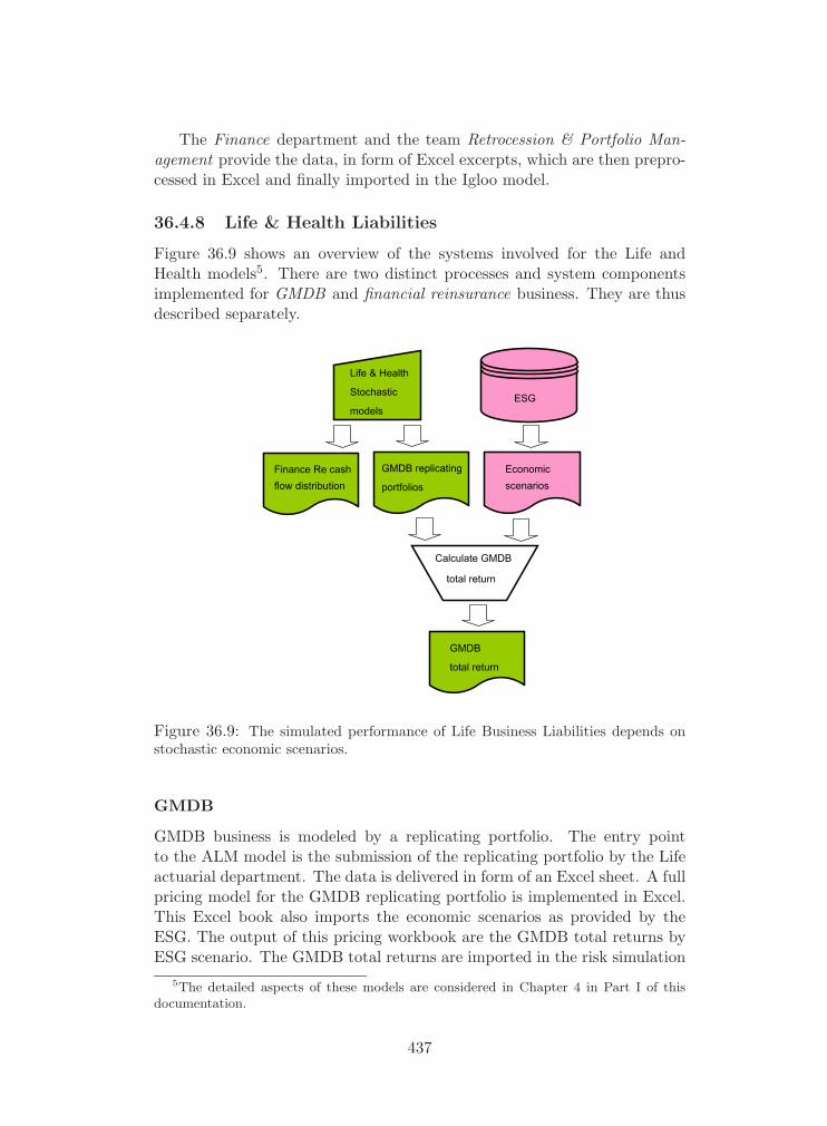
The Finance department and the team Retrocession & Portfolio Man-agement provide the data, in form of Excel excerpts, which are then prepro-cessed in Excel and finally imported in the Igloo model.
36.4.8 Life & Health Liabilities
Figure 36.9 shows an overview of the systems involved for the Life andHealth models5. There are two distinct processes and system componentsimplemented for GMDB and financial reinsurance business. They are thusdescribed separately.
GMDB replicating
portfolios
Life & Health
Stochastic
modelsESG
Economicscenarios
Calculate GMDB
total return
GMDB
total return
Finance Re cash flow distribution
Figure 36.9: The simulated performance of Life Business Liabilities depends onstochastic economic scenarios.
GMDB
GMDB business is modeled by a replicating portfolio. The entry pointto the ALM model is the submission of the replicating portfolio by the Lifeactuarial department. The data is delivered in form of an Excel sheet. A fullpricing model for the GMDB replicating portfolio is implemented in Excel.This Excel book also imports the economic scenarios as provided by theESG. The output of this pricing workbook are the GMDB total returns byESG scenario. The GMDB total returns are imported in the risk simulation
5The detailed aspects of these models are considered in Chapter 4 in Part I of thisdocumentation.
437
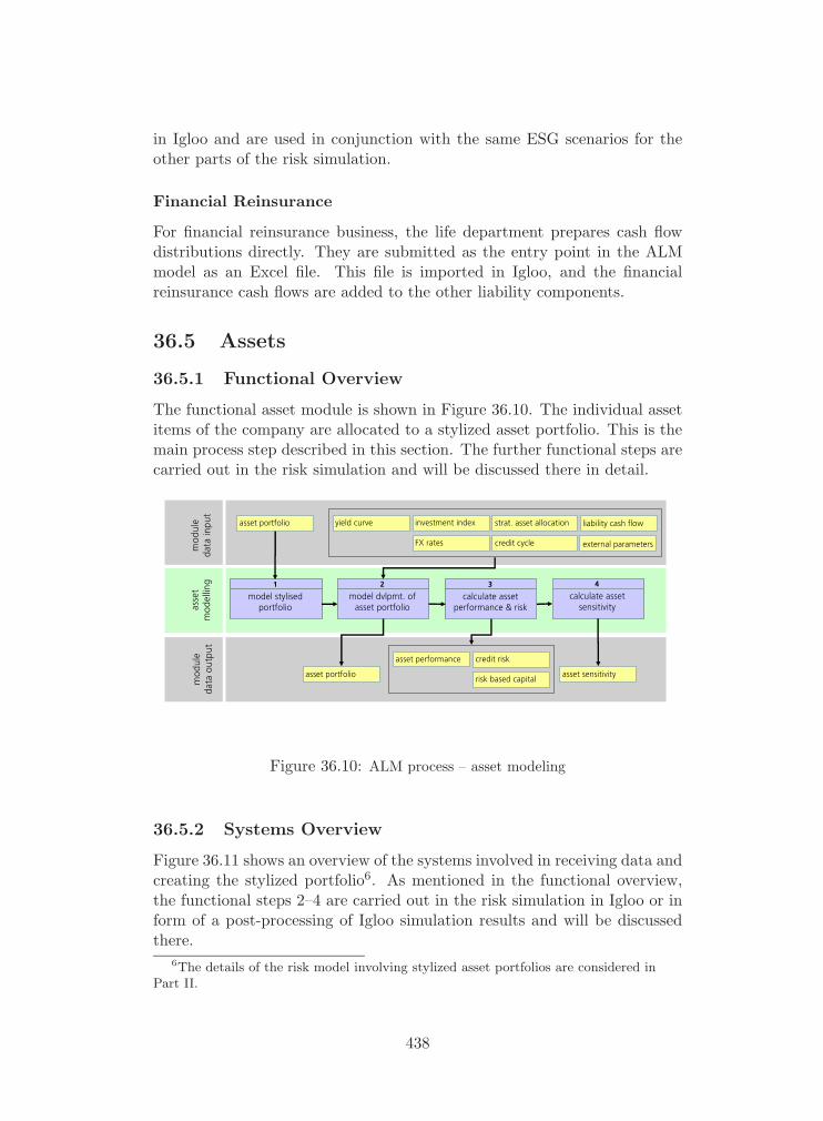
in Igloo and are used in conjunction with the same ESG scenarios for theother parts of the risk simulation.
Financial Reinsurance
For financial reinsurance business, the life department prepares cash flowdistributions directly. They are submitted as the entry point in the ALMmodel as an Excel file. This file is imported in Igloo, and the financialreinsurance cash flows are added to the other liability components.
36.5 Assets
36.5.1 Functional Overview
The functional asset module is shown in Figure 36.10. The individual assetitems of the company are allocated to a stylized asset portfolio. This is themain process step described in this section. The further functional steps arecarried out in the risk simulation and will be discussed there in detail.
1
model stylisedportfolio
2
model dvlpmt. ofasset portfolio
3
calculate assetperformance & risk
4
calculate assetsensitivity
mod
ule
data
inpu
tmod
ule
data
output
asset
mod
elling
strat. asset allocation
credit cycle
liability cash flow
external parameters
investment index
FX rates
asset portfolio yield curve
asset portfolio asset sensitivity
credit risk
risk based capital
asset performance
Figure 36.10: ALM process – asset modeling
36.5.2 Systems Overview
Figure 36.11 shows an overview of the systems involved in receiving data andcreating the stylized portfolio6. As mentioned in the functional overview,the functional steps 2–4 are carried out in the risk simulation in Igloo or inform of a post-processing of Igloo simulation results and will be discussedthere.
6The details of the risk model involving stylized asset portfolios are considered inPart II.
438
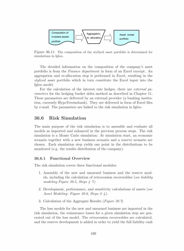
Composition of invested assets
portfolio
Aggregation,re- allocation
Asset model portfolio
Figure 36.11: The composition of the stylized asset portfolio is determined forsimulations in Igloo.
The detailed information on the composition of the company’s assetportfolio is from the Finance department in form of an Excel excerpt. Anaggregation and re-allocation step is performed in Excel, resulting in thestylized asset portfolio which in turn constitute the Excel input into theIgloo model.
For the calculation of the interest rate hedges, there are external pa-rameters for the hedging bucket delta method as described in Chapter 11.These parameters are delivered by an external provider (a banking institu-tion, currently HypoVereinsbank). They are delivered in form of Excel filesby e-mail. The parameters are linked to the risk simulation in Igloo.
36.6 Risk Simulation
The main purpose of the risk simulation is to assemble and evaluate allmodels as imported and enhanced in the previous process steps. The risksimulation is a Monte Carlo simulation: At simulation start, an economicscenario together with a new business scenario and a reserve scenario arechosen. Each simulation step yields one point in the distributions to bemonitored (e.g. the results distribution of the company).
36.6.1 Functional Overview
The risk simulation covers three functional modules:
1. Assembly of the new and unearned business and the reserve mod-els, including the calculation of retrocession recoverables (see liabilitymodeling Figure 30.5, Steps 4–7 )
2. Development, performance, and sensitivity calculations of assets (seeAsset Modeling: Figure 30.6, Steps 2–4 ).
3. Calculation of the Aggregate Results (Figure 30.7)
The loss models for the new and unearned business are imported in therisk simulation, the reinsurance losses for a given simulation step are gen-erated out of the loss model. The retrocession recoverables are calculated,and the reserve development is added in order to yield the full liability cash
439
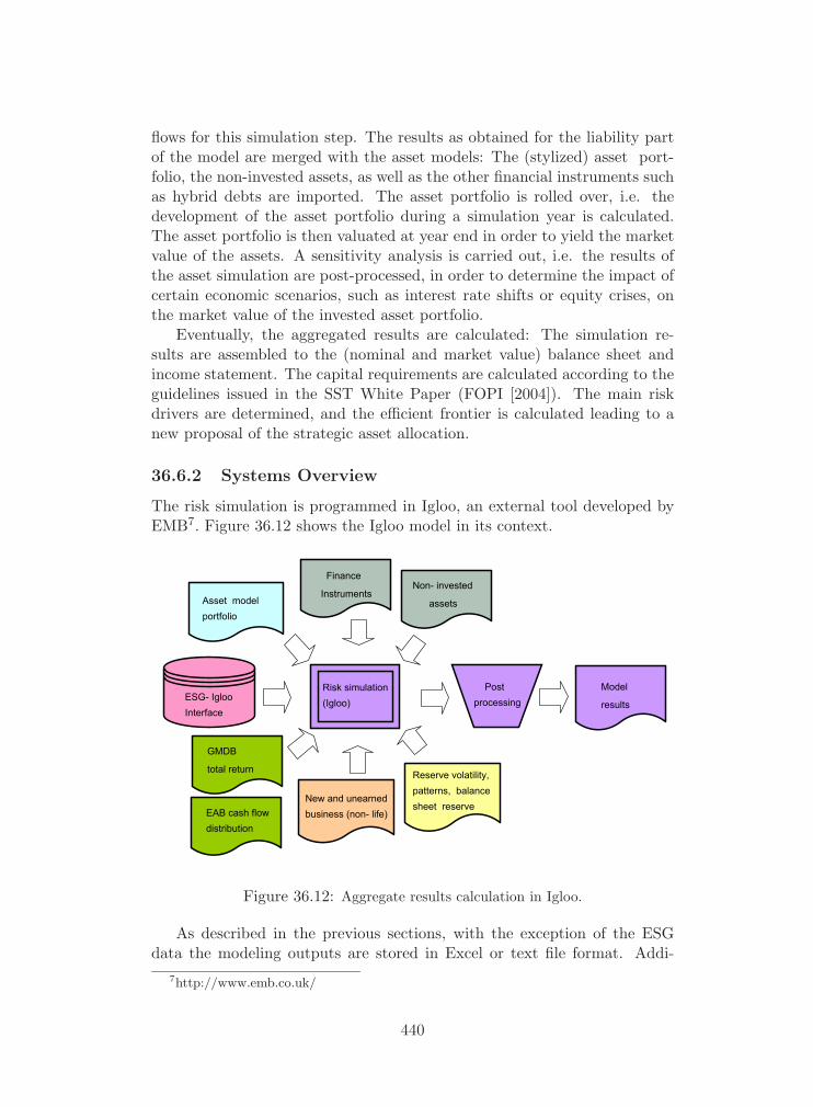
flows for this simulation step. The results as obtained for the liability partof the model are merged with the asset models: The (stylized) asset port-folio, the non-invested assets, as well as the other financial instruments suchas hybrid debts are imported. The asset portfolio is rolled over, i.e. thedevelopment of the asset portfolio during a simulation year is calculated.The asset portfolio is then valuated at year end in order to yield the marketvalue of the assets. A sensitivity analysis is carried out, i.e. the results ofthe asset simulation are post-processed, in order to determine the impact ofcertain economic scenarios, such as interest rate shifts or equity crises, onthe market value of the invested asset portfolio.
Eventually, the aggregated results are calculated: The simulation re-sults are assembled to the (nominal and market value) balance sheet andincome statement. The capital requirements are calculated according to theguidelines issued in the SST White Paper (FOPI [2004]). The main riskdrivers are determined, and the efficient frontier is calculated leading to anew proposal of the strategic asset allocation.
36.6.2 Systems Overview
The risk simulation is programmed in Igloo, an external tool developed byEMB7. Figure 36.12 shows the Igloo model in its context.
GMDB
total return
EAB cash flow distribution
Finance
InstrumentsNon- invested
assets
Postprocessing
Model
results ESG- Igloo Interface
Risk simulation (Igloo)
Asset model portfolio
New and unearned business (non- life)
Reserve volatility,patterns, balance sheet reserve
Figure 36.12: Aggregate results calculation in Igloo.
As described in the previous sections, with the exception of the ESGdata the modeling outputs are stored in Excel or text file format. Addi-
7http://www.emb.co.uk/
440

tional input to the risk simulation, such as the non-invested assets and thefinance instruments, are also stored in Excel or text file format. All data areimported in the risk simulation using Igloo links: Igloo is capable of readingsimple text or Excel files in tabular format and storing them in its marginals.Furthermore, Igloo provides an ODBC link via which SQL queries can besubmitted to the Microsoft SQL Server. This is the method which is usedto import ESG data in Igloo.
36.7 Presentation of Results
Igloo results comprise the CY and UWY risk based capital (RBC), targetcapital (TC), as well as asset returns and volatilities. Igloo exports resultsin the form of Igloo Reports. Igloo model output is post-processed andformatted with Excel. From there, the result tables are included in theALM and SST reports.
441
37
Architecture of NewDevelopments
In January 2007, a project was launched to re-implement the EconomicScenario Generator (ESG) as a state of the art software product. In thiscontext, a new strategy for developing the ALM systems landscape waselaborated, see ALM Information Architecture: Strategic Long-Term Vision(Burgi [2007]). For our description of the architectural strategy we exten-sively draw on the ideas, concepts and formulations originally presented inthat paper.
In the context of the general information disclosure policy being intro-duced in the reinsurance industry, with a special focus on the Swiss SolvencyTest (SST), new requirements on the ALM Information Architecture havebeen established, with an emphasis on the documentation of methods anddata together with the verification of a correct implementation of the re-lated processes. Data and methods have to be associated with a particularversion, correctness of implementation has to be guaranteed, and basic ITsecurity aspects have to be fulfilled. All these aspects are addressed by theALM Information Architecture.
37.1 Basic Architecture of Applications
The basic architecture of the applications (so far the ESG) is reduced to afew powerful components: the user interface, the object model including thecommunication layer, the mathematical kernel, and the ALM informationbackbone. Figure 37.1 graphically displays the basic application architec-ture.
The object model is at the centre of the architecture. It is used totransfer data from the user interface to the mathematical kernel and to thedata base. It consists of simple data objects which can get and set properties.The communication layer enables to transfer, load, and save data from and
442
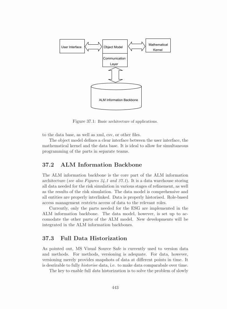
ALM Information Backbone
User Interface Object Model
Communication
Layer
Mathematical Kernel
Figure 37.1: Basic architecture of applications.
to the data base, as well as xml, csv, or other files.The object model defines a clear interface between the user interface, the
mathematical kernel and the data base. It is ideal to allow for simultaneousprogramming of the parts in separate teams.
37.2 ALM Information Backbone
The ALM information backbone is the core part of the ALM informationarchitecture (see also Figures 34.1 and 37.1). It is a data warehouse storingall data needed for the risk simulation in various stages of refinement, as wellas the results of the risk simulation. The data model is comprehensive andall entities are properly interlinked. Data is properly historised. Role-basedaccess management restricts access of data to the relevant roles.
Currently, only the parts needed for the ESG are implemented in theALM information backbone. The data model, however, is set up to ac-comodate the other parts of the ALM model. New developments will beintegrated in the ALM information backbones.
37.3 Full Data Historization
As pointed out, MS Visual Source Safe is currently used to version dataand methods. For methods, versioning is adequate. For data, however,versioning merely provides snapshots of data at different points in time. Itis desrirable to fully historise data, i.e. to make data comparabale over time.
The key to enable full data historization is to solve the problem of slowly
443

changing dimensions: Codes such as line of business, business unit etc. varyover time. Codes including structural elements (e.g. hierarchical grouping),validity of codes (code versioning), migration of codes (management of suc-ceeding codes) etc. have to be administered with utmost care in order toguarantee full data historization. It will thus be possible to link or comparedata sets provided at different points in time. A clever code administrationsystem is the foundation of the ALM information backbone.
37.4 Separating Data from Methods
Technologies such as Excel have the disadvantage that they couple datatighlty to methods. It is only possible with significant efforts to get Excelto perform the same calculation with the same code for multiple data sets.
The downside of linking data and methods is that tools are difficult totest; one of the preconditions to a high testability is the ability to build atest suite, which requires full decoupling of data from methods.
In the ALM information architecture, data is only foreseen to be storedon the ALM information backbone. The methods are provided by the ap-plications and are thus fully separated from the data.
37.5 Design Principles
Four design principles of overarching importance shape the long term strat-egy and the formulation of the information architecture:
1. Extensibility: Allowing for an adaption to new methods as the method-ology progresses with time, easily adapting to changes in the datamodel when new or higher quality data become available. The datamodel, the modules, as well as the user interfaces evolve with time.
2. Maintainability: Low maintenance and the ability of keeping up withthe changes for example in data formats. Flexibility, in terms of aswift implementation, with respect to a varying combination of dataand methods.
3. Testability: The ability to test the IT components for errors and mal-functions at various hierarchy levels, using an exhaustive set of prede-fined test cases.
4. Re-usability: The ability to recombine programming code and systemparts. Each code part should be implemented only once if reasonable.Thus, the consistency of code segments is increased significantly.
444
37.5.1 Extensibility
The methodologies developed in financial modeling constantly evolve. Moreand higher quality data become available over time, and methods becomemore sophisticated. Changes can be significant, and they have impacts onthe ALM Information Architecture, such as the data model, the methodsmodules, and the user interfaces.
It is not possible to design a universally extendable model and system.Nevertheless, good design techniques can provide a minimum standard inuniversal extensibility. A consistent separation of data and methods, whichhas so far been achieved only for the ESG, will deliver a substantial gain inthis respect.
In order to develop models and systems it must be anticipated whichextensions will likely be needed later on, and the design has to be chosenappropriately. In the case of unanticipated changes it is important to en-sure that the extension is cleanly implemented, and that code segments arerefactored appropriately.
Currently, the modules provide limited support for extensions. Thisimplies that a change in the modules potentially leads to major rebuilds.The current model implementation is strongly linked to technology.
Special care has to be taken regarding extensions which will be developedby external partners. It is important to guarantee a stable and clean APIwhich will underlie a clean change management process.
37.5.2 Maintainability
In the current ALM infrastructure, substantial efforts have to be invested inthe maintenance of data and systems. Due to the representation in Excel,the data modeling is restricted to two-dimensional tables. This leads tosubstantial efforts maintaining them.
Maintainability of data can be improved significantly by using appropri-ate technology. The example of ReCube (which is a hypercube on the re-serving database CORE) shows an intelligent way of maintaining data fromthe reserving process. Data inputs can be conveniently linked in Excel, andthe update of the sheets is much better supported in this process.
An important aspect to maintainability is a clear data and methods ver-sioning. The ALM process security can be significantly enhanced by combin-ing different data and methods versions. For instance, the new methods canbe developed using the old data in order to assess the quantitative impactof the changes.
37.5.3 Testability
To test an IT component for its functionality in a reliable manner, severallayers of test cases are needed. The lowest level is the unit test layer. Ideally,
445

each method has a corresponding set of test cases which is as exhaustive aspossible. Most of the defects are then detected on the unit test level. Thisis where they can be fixed at very low cost.
Above the unit test level is the component test layer. The componenttests typically cover a whole module. They can be created synthetically orcan be chosen from productive data sets. The component test suite shouldcontain both a simplified and a real complexity set of test cases which arewell known. They can ideally be used for developing new methods andshould thus be well studied.
The last test level is the integration test layer. It covers the integrationof modules with each other and focuses on the interfaces, i.e. the transferof data, evolution of data after application of multiple modules etc.
If all these test layers are created and maintained, the error potentialduring development and refactoring of code can be reduced significantly.Therefore, testability enables to fulfill the design criteria extensibility andmaintainability.
The issue of testability is also addressed by the corporate software devel-opment and application management processes as described in Section 35.1.
37.5.4 Re-usability
Smart reuse of code and system parts leads to a clear design and supportsall other design criteria. Several aspects of re-usability are important:
1. Obtain full consistency : If components or modules are implementedmultiple times, experience shows that the implementations will divergesooner or later. It is therefore essential to elect and label one currentversion of each concept, method, data set etc., and to keep the imple-mentation unique. This implies that the design of modules supportsusage in multiple contexts.
2. Keep specification, implementation and documentation close: In manycases, it is possible to combine specification, implementation and doc-umentation in one place. For instance, a conceptual data model iscreated and kept as the unique place for change. From the conceptualdata model, a physical model can be generated automatically. Fur-thermore, an object model can also be generated automatically fromthe conceptual data model (object oriented communication layer to beused, e.g., between user interface and mathematical kernel). A doc-umentation of the data model can be compiled from the conceptualdata model. This allows for keeping specification, implementation anddocumentation in sync at all times without additional maintenanceeffort. The concept has been fully realized for the economic scenariogenerator.
446

3. Provide basic components for new modules: If code is designed forre-use, a large collection of tools will be gathered over time. It willbe easy to generate new modules making use of this collection. Thus,calculation requirements to Financial Modeling can be met at best.
4. Run models from the past: It should be possible to combine differentmodel and data versions. This allows for assessing the effect of methodand data changes and optimized auditability and reproducibility ofresults.
Even though re-usability may appear as an obvious design criterion, it isnot always desired. Modules and data need to be well encapsulated so thatthey can be changed independently. In some of these cases, re-usability maynot be the right criterion to optimise, and code duplication may not alwaysbe a bad choice. It is important to find the right balance between reuse andencapsulation.
37.6 Security
All newly built parts of the ALM information architecture will incorporaterole-based access management. The ability to read, create, update, anddelete data entities will be given according to the roles in the ALM Process.
Entities which are used for production of the ALM or SST reports, orwhich are communicated otherwise internally or externaly, can be locked.Locks are cascading, i.e. when locking a data entity, all entities which feeddata into this entity must be locked as well. When an entity is locked, thedata becomes read-only, and it is not possible to delete it. An audit trailcan thus be guaranteed.
447

38
Appendix
We list the IT systems and their owners. For commercial software tools, wealso list (in braces) the company from which the licence or the applicationwas purchased.
IT System Ownership
GPT – Global planning toolBusiness projections during the plan-ning cycle of the company
Financial Planning & Analysis
MARS – Model for analyzingreinsurance submissionsPricing tool for non-life treaty business
Actuarial – Non-Life
PhobosManipulation of aggregated risk vari-ables and modeling-basket dependen-cies in non-life treaty business
Actuarial – Non-Life
GCDP – Global cat data platformAggregation of natural catastrophe riskand risk accumulation control
Natural Hazards
ResQReserving tool, commercial software(EMB Consultancy)
Actuarial – Non-Life
continued on next page
448

IT System Ownership
CORE – Converium reserveestimatorReserve analysis tool and database
Actuarial – Non-Life
ReCubeAnalyzing reserving data, producingreserve triangles
Financial Planning & Analysis
ESG – Economic scenariogeneratorGenerating stochastic economic scenar-ios
Financial and Rating Modeling
FED – Financial and economicdatabaseProviding historic financial and eco-nomic time series
Financial and Rating Modeling
IglooStochastic simulation of assets and li-abilities. Commercial DFA software(EMB Consultancy)
Financial and Rating Modeling
449

IX
Final Remarks
450

In July 2008, the first SST report of SCOR Switzerland will be deliv-ered to the FOPI. It is a reflection of the outcome of SCOR Switzerland’sinternal model that was to a good extent already in use at Converium fora couple of years and constituted the basis of various ALM reports of Con-verium. However, to fulfill the further requirements of the SST, substantialenhancements of the internal model have been recently built in. This re-lates to a stricter “pure” legal entity view including internal retrocession andparental guarantees, a much more comprehensive documentation regardingsystems, processes and the various models. However, several limitations arestill associated with various parts of the internal model (as mentioned in thesections on model limitations in this document). This also refers, last butnot least, to the modeling of management rules concerning dividends, capi-tal management, strategic asset allocation, business mix and volume duringthe business cycle and global risk mitigation. We aim to continuously im-prove the internal model regarding those limitations and fully understandthe potential need for additional models that will be always a consequenceof writing new lines of business, investing in new types of investments etc.This document will therefore be updated to the extent those enhancementsmaterialize in the internal model.
Acronyms 452
Index 456
References 481
451
Acronyms
A
AAD Annual aggregate deductibles.
AAL Annual aggregate limits.
ACM Application change management.
ALM Asset liability management.
ATP Application testing process.
B
BoD Board of Directors.
BS Balance sheet.
C
CDS Credit default swaps.
CEO Chief Executive Officer.
CFO Chief Financial Officer.
CIO Chief Investment Officer.
CoCM Cost of capital margin.
COO Chief Operating Officer.
CORE Converium reserve estimator.
CPI Consumer price index.
CRO Chief Risk Officer.
CTA Currency translation adjustment.
CY Calender year.
452

D
DFA Dynamic financial analysis.
dvlpmt Development.
E
ECS Executive Committee Switzerland.
EDF Expected default frequency.
ESG Economic scenario generator.
EUR Euro.
F
FED Financial and economic database.
Finance Re Financial reinsurance.
FinMod Financial Modelling.
FOPI Federal Office of Private Insurance.
FX Foreign exchange.
G
GAUM Global Aerospace Underwriting Managers.
GCDP Global cat data platform.
GDP Gross domestic product.
GMDB Guaranteed minimum death benefit.
GPT Global planning tool.
I
ILF Increased limit factor.
K
KMV Moody’s KMV.
453

L
LE Legal entity.
LGD Loss given default.
LoB Line(s) of business.
M
MARS Model for analyzing reinsurance submissions.
MDU Medical Defense Union.
MKMV Moody’s MKMV.
MSCI Morgan Stanley Capital International.
MVM Market value margin.
N
Nat cat Natural catastrophe.
NCB No claims bonus.
NFS Network file system.
Non-prop Non-proportional.
NPV Net present value.
O
ODBC Open database connectivity.
OLAP Online analytical processing.
ORP Optimal replicating portfolio.
P
Prop Proportional.
Q
Q1 First quarter.
Q3 Third quarter.
454

R
RAC Risk adjusted capital.
RBAM Role-based access management.
RBC Risk-based capital.
ROP Roll-up policies.
S
SAA Strategic asset allocation.
SDLC Software development life cycle.
S&P Standard & Poors.
SQL Structured query language.
SST Swiss solvency test.
T
TRAC Time and risk adjusted capital.
U
USD US Dollar.
UW Underwriting.
UWY Underwriting year.
455

Index
Accident and healthmodel basket, 59
Acquisition and maintenance costs,see internal administrativeexpenses
Adjusted estimated ultimate lossratio, see as-if adjustments,proportional pricing
Administrative expenses, see inter-nal administrative expenses
Age-to-age factordefinition, 95
Aggregationaggregate distributions, 72natural catastrophe, aggregate
exposure, 83Aggregation of risks
aggregation of basket models,62
aggregation of patterns by modelbasket, 51
bottom-up aggregation, 148, 150capital allocation for a port-
folio dependency tree, 172,180
dependency structure, aggre-gation for new business, 59
dependency structure, aggre-gation for run-off risk, 99
dependency structure, aggre-gation methodology, 49
dynamic aggregation process,xvi
limitations of the one param-eter copula family, 144
partial models in life and health,
121risk input and balance sheet
output, 332suitability of the dependency
tree, 150the default basket model, 59
Agribusinessmodel basket, 59
Allocated capital costscalculatio of the treaty NPV,
73Allocation
valuation of insurance liablili-ties, 10–13
Allocation of capitalfor a portfolio dependency tree,
180–184pricing capital allocation, 168–
191top down allocation, 148
Allocation of costs to financial in-struments, 12
ALM and SST process, 358–405ALM information backbone, 443ALM systems, 415, see IT systems,
see also ALM processAmortization margin
Life & Health business, 108Analytic distributions, 68Arbitrage
arbitrage-free consistency in boot-strapping scenarios, 204,220
no-arbitrage pricing, 11Archimedean copulas, 161–165Architecture of IT systems, 416–
456
420As-if adjustments
proportional pricing, 67Asset allocation, see strategic as-
set allocation, 235, 243, 247,288–290, 451
ALM process landscape, 358market value share of an asset
portfolio, 289SST systems, 430
Asset indexLife & Health business, 39, 124
Asset riskLife & Health business, 105
Attractor copula, 158Attritional losses, 66, see pricing,
67cat model, 146definition, 66model limitations, 146
Autoregressive conditional heteroskedas-ticity, 209
Aviationexposure pricing, 69, 74, 76market model, 75–76non-proportional and large loss
models, 68
Back testing, stress testing, see pric-ing, see economic scenar-ios
Balance sheet solvency, see also sol-vency capital requirement
as distinct from cash flow sol-vency, 19
Basis risk, 9, 13, see replication,14–16, 39
assumption of vanishing basisrisk for liquidly traded in-struments, 30
assumption of vanishing basisrisk in GMDB, 31
cash flow mismatch, 16cash options, 15
definition, 25one-year max cover, 16reserve deficiency, 24the market value margin (MVM)
as the value of the basisrisk, 25
value of the basis risk, 19Basket hierarchy
portfolio dependency, 149Basket model, 59–103
aggregation of basket models,62
allocation of capital for a port-folio dependency tree, 180–184
basket specific models, 62copulas, 154–158default basket model, 59dependency measures, 158–161explicit and implicit dependency
models, 153portfolio dependency tree, 148–
168suitable portfolio decomposi-
tion, 148–153Basket shortfall ratios, 35
proxies, 36proxies, 36
Baskets, see basket modelBest estimate of future cash flows,
see ReplicationBond exposure, 77
credit and surety exposure pric-ing, 77
Bond portfolio management, see mar-ket risk, 251–276
Bond portfolios with credit risks,320–321
Bond yields, 306Bootstrap, see market risk, 203–
245calibration, 235–236dependency structure, 213detrending scenarios, 211
457

economic variables, 218–235equity indices, 234–235fat tails of distributions, 215–
218foreign exchange rates, 232–233gross domestic product, 233heteroskedasticity, 213–214inflation, 229–230interest rate forwards and fu-
tures, 219–221interest rates and inflation, 230–
232mean reversion, 211–212noise in scenarios, 210out-of-sample backtesting, 237–
241overview of the method, 208–
209results and testing, 235–245seasonality in scenarios, 210–
211time steps, high frequency ob-
servations, 209–210yield curve, 228–229
Bornhuetter-Ferguson, see run-offbusiness
Bottom-up aggregationportfolio dependency, 148
Calculation of SCR, 29Calendar year patterns, see pat-
ternsCalibration
GMDB replicating portfolio, 131–132
of economic scenarios, 235–236of the copula between life and
non-life risks, 139of the dynamic credit risk model,
317–318Capital costs, 185–186Capital fungibility, see fungibility
of capital
Capital margin, 9, 21, 22, 24, 25,28
Capital market riskLife & Health business, 106
Case reservesdefinition, 93
Cash flow discounting and devel-opment patterns, non-lifeinsurance liabilities, 50–56
Cash flow discounting, risk free, 8Cash flow management, see mar-
ket risk, 287–291Cash flow mismatch
one-year max cover, 17Cash flow modeling
trend risk, 111Cash flow solvency, 19Cash-in option, see replicationCash-out option, see replicationChain ladder, see run off businessChain ladder factor
definition, 95Claim supporting capital
foreign exchange risk calcula-tion, 292
Claims developmentcumulative paid loss pattern,
53split into payment and reserves,
52Clash potentials
natural catastrophe modeling,80
Clayton copula, 161–165aggregation of baskets in port-
folio dependency tree, 62between life and non-life risks,
139Co-monotonicity copulas, 156Coefficients of tail dependency, 158Coherent risk measure, see expected
shortfalldefinition, 173
Collective model, see pricing
458
Common account protection, seepricing
Compound Poisson model, see pric-ing
Concordance order for copulas, 157Consistent scenarios, see economic
scenario generatorContingent capital, 349Contingent claims, 10Conversion formula: credit spreads
and defaults, 308–312Conversion of assets
SST solvency condition, 25Convex risk measure, see utility
functionCooperative game, 12Copulas, 154–158
Archimedean Copulas, 161–165Clayton Copula, 161–165
Cost of capital, 16–23total discounted capital costs,
39Cost of capital margin, see insur-
ance riskCounter-monotonicity copulas, 156Credit and surety
exposure pricing, 76–78portfolio model, 78–80
Credit cycle, see market riskCredit default swaps, 306Credit risk, 300–322
ALM and SST process, 358–405
ALM process modules, 368ALM process, credit cycle and
credit spreads, 372bond portfolios with credit risk,
320bond yields, 306–312calibration of the credit risk
model, 317–318completeness of the model, 332conversion formulas, 308–312corporate bonds, 300–302
credit and surety line of busi-ness, 320
credit cycle, 199credit default swaps, 306credit default swaps inddices,
306credit risk level, 305, 306, 308credit risk level as an economic
variable, 301credit risk level, creditworthi-
ness of companies, 313credit risk level, historical be-
havior, 313credit risk levels, historical time
series, 313credit risk levels, rating classes,
312credit spreads, 303–321creditworthiness vs. individ-
ual rating, xvcreditworthiness, asymmetric dif-
fusion, 312debt valuation, 349default of the cedent, financial
reinsurance, 108default probabilities, 306–307default scenarios, 109dependence between liabilities
and credit risk, 320dependence between market and
credit risk, 319–320dependence between market risk
and credit risk, credit cy-cle, 313
dependency between credit riskand general asset risk, 104,109
dependent companies, credit riskdynamics, 318–319
dynamic behavior, 312–319financial reinsurance, xiv, 104funds held by reinsureds, 302granted credit limit, 76individual firms, 314–317
459
invested assets and credit risk,303
IT implementation, 413–449life and health liabilities, 109limitations of the credit risk
model, 322loan to the cedent, financial
reinsurance, 105major risk category set by FOPI,
xiiimarket risk and credit risk, sep-
aration in bond portfolios,321
portfolios, credit risk dynam-ics, 318–319
rating agencies, 322rating classes, 308, 310–311rating migration, 314–317ratings, 307–308reinsurance assets, 140reinsurance company, credit risk
modeling, 320–321retrocessionaires and other oblig-
ors, modeling the credit risk,321
variables describing credit risk,306–312
yield curves, 308–312Credit risk level, see credit riskCredit risk of a rating class, 312–
314Credit spreads, see credit risk, 306
and defaults, 303–321Creditworhiness, see credit riskCurrency translation adjustment,
284
Data errors when using the Mackmodel
the quest for an alternative ap-proach, 98
Data requirements and parameters,see insurance risk
Debt, 349
Decompositionportfolio decomposition, see bas-
ket modelDecomposition of the liability port-
folio, 29Deductible rebate curves, see pric-
ingDefault basket model, see basket
modelDefault option, see replicationDefault probabilities
credit spreads, 306–307Defaultable cash option, see repli-
cationDeferred policy acquisition costs,
346Dependence of economic variables,
see economic scenariosDependency measures, 158–161Dependency models, see basket modelDependency structure, see aggre-
gation of risks, see also in-surance risk, market risk,credit risk, life and health
Dependency tree, see basket modelDependent companies
credit risk dynamics, see creditrisk
Design of IT systemsdesign principles, see IT im-
plementationDeterministic estimates
premiums and expenses, 92Detrending a time series, see eco-
nomic scenariosDevelopment patterns, 50–56Development triangles, 93–97Diffusion
asymmetric diffusion of cred-itworthiness, see credit risk
DisabilityLife & Health business, 104
Discounted best estimate of the li-abilities, 23
460
Discounted outstanding reserves, 29,30
definition, 24for model baskets, 36
Discounted reserves, see economicbalance sheet
Disjoint sub-portfoliosportfolio dependency, 149
Distorted probability measure, 189Distribution-free model
Mack assumptions, 95Diversification benefit, 29, 33, 34,
38Duerr method, 98Dynamic portfolio, 11Dynamics of credit risk, see sce-
narios
Earned business at time tnon-life insurance model, 42
Earthquakenatural catastrophe modeling,
81, 82, 85, 86, 88, 89Economic balance sheet
aggregating risk inputs, 332balance sheet solvency, 24data entities in the ALM pro-
cess, 394, 395dependencies and aggregation
of risk factors, xiiidiscounted reserves, 23economic shareholders equity,
xiiifocus of SST report, xiimarket consistent valuation of
insurance liabilities, 9one-year max cover, 21optimal replicating portfolio,
20run-off liabilities, 26run-off liabilities, diversification
gain, 26run-off perspective, SST, 27
valuation by perfect replication,12
Economic innovationdependency structure of inno-
vations, 213expectation of interest rates and
inflation, 230–232forward interest rates, 221–228
Economic risks, see market risk,198–245
Economic scenario generator, 199–245
calibration, 235–236dependency structure, 213detrending, 211economic variables, 218–235equity indices, 234–235fat tails of distributions, 215–
218foreign exchange rates, 232–233gross domestic product, 233heteroskedasticity, 213–214inflation, 229–230interaction of interest rate with
inflation, 232interaction of interest rates with
inflation, 230interest rate forwards and fu-
tures, 219–221mean reversion, 211–212noise, 210non-parametric method, boot-
strap, 203–245out-of-sample backtesting, 237–
241results and testing, 235–245seasonality, 210–211time steps, bootstrap, 209–210yield curve, 228–229
Economic scenarios, see market risk,199–245
bootstrap, 203–245calibration, 235–236dependency structure, 213
461
detrending, 211economic variables, 218–235equity indices, 234–235fat tails of distributions, 215–
218foreign exchange rates, 232–233gross domestic product, 233heteroskedasticity, 213–214high frequency observations, 209–
210inflation, 229–230interest rate forwards and fu-
tures, 219–221interest rates and inflation, 230–
232mean reversion, 211–212noise, 210out-of-sample backtesting, 237–
241results and testing, 235–245seasonality, 210–211yield curve, 228–229
Economic variables, 218–235equity indices, 234–235foreign exchange rates, 232–233gross domestic product, 233inflation, 229–230interaction of interest rates with
inflation, 230–232interest rate forwards and fu-
tures, 219–221yield curve, 228–229yield curve simulation, 236
Economic zones, 198, see marketrisk
Emerging risks, 327Empirical distribution
economic scenarios, 215–218end baskets
portfolio dependency, 149Engineering
model basket, 59Engineering line of business
model basket, 59
Equity indices, 234–235economic scenarios, 218–245
Equity portfolio modeling, see mar-ket risk, 277–286
Estimated reservesdefinition, 93
Estimated ultimate lossesdefinition, 93
Estimation error versus parametererror
Chain ladder model, 96Euler principle, 173–180Event ground up damage ratio
natural catastrophe modeling,83
Expected cash flow replicating port-folio, 23–24, see replica-tion
Expected default frequency, 77, 306Expected loss ratio, see pricing, see
pricingExpected shortfall, xii, 179, 180,
185, 191, 349ES principle of capital alloca-
tion, xiv1% safety level, 27application to the NPV of the
technical result, 171capital computation and extreme
risks, 293coherent risk measure, 173economic balance sheet, 332economic value of a legal en-
tity, 347efficient frontier, 370Euler principle, 171future one-year changes, 98impact of risk level on the de-
fault option, 21law invariant risk measure, 39proxy for shortfall ratio, 98reserve development, 347restriction on the states of the
world, 179
462
risk contribution to the ES, re-sults of Kalkbrener, 175
risk tolerance, 171spectral risk measure, 168spectral risk measure and Eu-
ler principle, 173stand-alone ES of NPV, 74tail based risk measures, 215target capital, 351valuation of assets, 343valuation of liabilities, 347VaR, Tail VaR, 173weight function, 176
Experience account balanceLife & Health business, 108
Experience pricing, see pricingExplicit Dependency
between Economic Variables andLiabilities, 168
Explicit dependencybetween economic variables and
liabilities, 165Explicit dependency model, see bas-
ket modelExposure curve, see pricingExposure curves, see pricingExtensibility
design principles for IT systems,see IT implementation
External expensesnew business, 31run-off business, 31
External retrocession, see risk trans-fer, 37, 38
ALM modules, 369requuirements on non-life model,
48Extratropical storm
natural catastrophe modeling,84, 85
Fat tails of distributions in eco-nomic scenarios, see sam-ple size
Filtered bootstrapGARCH filter, 214
Filtration, 8Financial instruments
Bloomberg fair-market yield curves,219
allocation of costs, cooperativegame, 12
candidate assets for GMDB,calibration and replication,107
contingent claims, 10default, cash-in, cash-out, 14hybrid debts, 440information given to the com-
pany by banking institu-tions, 343
interest rate based instruments,220
interest rate hedges, 246liquid instruments, 10look-back options, 121no-arbitrage pricing, 11non-traded instruments, 10notation and conventions, 8pseudo replication, 14structured notes, 343transaction costs, 12valuation, 9
Financial modulenatural catastrophe modeling,
89Financial reinsurance, 108–109
definition and exposure, 108dependency structure, 109stochastic model, 108–109
Fluctuation risk, 32, 111–120choice of parameters, 117–120definition and exposure, 111–
112determination of risk clusters,
115–117stochastic modeling, 112–115technical modeling, 120
463

Life & Health business, 105Foreign exchange
economic scenarios, 218–245Foreign exchange rates, 232–233Foreign exchange risk, see market
risk, 292–294claim supporting capital, 292
Frechet-Hoeffding bounds, 158Frequency-severity model, see pric-
ingFrequency/severity
large loss models, 66Fungibility of capital, 332–341Future time series, see economic
scenarios
GARCH process, 200, 213–214GAUM
model basket, 59General mortality death benefit, see
GMDBGeographic value distribution model
natural catastrophe modeling,87
GMDB, 106–107calibration of the replicating
portfolio, 131–132definition and exposure, 106–
107projecting the replicating port-
folio, 135–136replicating assets, 124stochastic modeling, replicat-
ing portfolio, 121–136Gross domestic product, 233Ground motion
natural catastrophe modeling,86
Ground-motion attenuation modelnatural catastrophe modeling,
85Gutenberg-richter law
natural catastrophe modeling,86
Hailstormnatural catastrophe modeling,
85Hazard module
natural catastrophe modeling,84
Hazard uncertaintynatural catastrophe modeling,
82Heavy tail distribution, see mar-
ket riskHeavy tailed loss distributions, see
pricingHedge funds, 345Hedging component in cash flow
management, 291Heteroskedasticity
GARCH process, 213–214Hierarchy of model baskets
portfolio dependency structure,149
Historical lossesAs-if adjustments, 70
Historical time series, see economicscenarios, see also ALMprocess
Historical treaty results, see pric-ing
Historization of data, 443–444
IBNRdefinition, 93
ILF exposure curves, 71Imperfect replication, see replica-
tionImplementation
of IT systems, see IT imple-mentation
Incomplete trianglesshortfalls of the Mack model,
98Increased limit factor curves, see
pricingIndependence copula, 156, 158, 238
464

Individual model, see pricingInflation, 229–230Information
rebalancing in the cash flow man-agement module, 281
simulation using information onparental guarantees, 349
simulation using information onretro structure, 349
address information, 88as-if adjustments, 67at start and end of simulation
in asset modeling module,279
available information, 8, 16, 17,20, 23, 24
chain ladder factors, 96company specific credit risk and
economic scenario genera-tion, 304
contract information in expo-sure pricing, 79
contracts with banking part-ners, 248
credit rating of a firm, 307databases on company specific
credit information, 305default option, 17distinction of risk classes, 116event loss tables, 82exchange of information between
asset and liability model-ing modules, 287
exchange of information betweenasset models, 251
exchange of information betweenbond portfolio componentand its sister component,264
exposure information, 65, 74,87, 154
external cash flow managementmodule, 264
external information for an as-
set modelling module, 263extremal dependencies, 99first development year, 99forbidden circular information
in the asset modeling mod-ule, 264
from yield curves to forwardrates, 220
future liability cash flows, 20geographical value distribution,
87growth assumptions, 385hazard information, 80historical discount rate changes,
69information for new business,
31information gained within a year,
20information needed for cash flow
management, 289information on innovations, 207information on the location level,
87information on the use of land,
85initial asset component, 290input data in the Life model,
117interpolation in the asset model,
260lack of information about FX
rates, 264large-loss information, 66, 67long duration life business, 31market and credit information
for dependency structuremodeling, 109
most recent underwriting year,94
necessary information for a sim-ulation step in asset model,256
new information revealed dur-
465

ing first development year,63
occupancy type, 88paid and reported losses, 55perfect replication, 11premium and loss ratio in ex-
posure pricing, 78pricing information used for mod-
eling new business, 44reduction of uncertainty, 171,
185reliability of information, port-
folio uncertainty, 82renewal information, 64required information on bands
in exposure pricing, 70reserving data, 45simulation using information on
parental guarantees, 372standardized aviation question-
naire, 74tail of loss, 78temporality of capital, 15unbiased replication, 24underwriting information in the
Life model, 118Information available at time t, 8Innovation, see economic innova-
tionInsurance liabilities
cash flows, 287–291finance re, see financial rein-
surancegeneral mortality death bene-
fit, see GMDBlife and health, see life and health,
104–136non-life, 103, see non-lifevaluation, 9allocation principle and pric-
ing of liabilities, 13cash flow replication, 45cash flows from and to the in-
surance liabilities, 251
contingent claims valuation, 10costs and expenses, 100economic balance sheet, 332liabilities and the modes of val-
uation, 348not deeply and liquidly traded,
13pension liabilities, 349replication, 9selection of an optimal repli-
cating portfolio ORP, 31stochastic model for SST, 63
Insurance risk, 8–191aggregation, run-off risk, 59–
62, 99ALM and SST process, 358–
405ALM process modules, 368aviation market model, 75–76capital allocation and pricing,
168–191capital costs, 185capital, risk adjusted, 186–191capital, time and risk adjusted,
186–191cash flows of liabilites and as-
sets, 287–291catastrophic events, 105Clayton copula, 161–165completeness of the model, 332concentration risk, 105contingent claims, 10copulas, 154–158cost of capital margin approach,
9, 21data requirements, 48, 58, 76data requirements and param-
eters, 100default scenarios, life and health
liabilities, 109dependence between liabilities
and credit risk, 320dependency between credit risk
and general asset risk, 109
466

dependency between default ofretrocessionaires and nat-ural catastrophe, 322
dependency between life andnon-life insurance risks, 138–139
dependency measures, 158–161dependency models, 152–168dependency structure between
model baskets, aggregationmethodology, 49
dependency structure betweenmodel baskets, portfolio de-pendency tree, 57, 148
dependency structure in bas-ket specific models, 58
dependency structure, life andhealth, 120
dependency structure, run-offrisk, 59–62, 99
Euler principle, 173–180expected cash flow replicating
portfolio, 14, 23finance reinsurance, 104, 108–
109fluctuation risk, 105, 111–120GMDB, 104, 106–107immateriality of insurance risk
for GMDB, 108imperfect replication, 13implementation and IT systems,
431independence between fluctu-
ation risk and reserve risk,115
independence between fluctu-ation risk and trend risk,111, 115
independence between trend riskand other risk categories,120
IT implementation, 413–449IT implementation of model bas-
ket dependencies, 431
law-invariant risk measure, 15liability cash flows, 287–291liability model and foreign ex-
change risk, 292–294life and health, structure and
types of business, 104life insurance liabilities, 104–
136limitations, 143–147long duration business, 104long term insurance risk, 105,
109main categories, xiiimajor risk category set by FOPI,
xiiimarket consistent valuation, 10,
15model for internal administra-
tive expenses, 100–103mortality, GMDB, 106natural catastrophe modeling,
80–91, 145–146new business model, 56–63non-life insurance liabilities, 103one-year change vs. ultimate
change, 62–63, 97–98optimal replicating portfolio,
13perfect replication, 10policy holder behavior, GMDB,
106portfolio decomposition, 148portfolio dependency tree, 148–
168price of one-year max cover,
18pricing models for new busi-
ness, 63–74quota share retrocession agree-
ment, 336recoveries modeled in Igloo, 436regression model on recover-
ies, 141, 436reinsurance assets, 140
467
retrocession, 332–341retrocession and risk mitiga-
tion, 140–142retrocession of insurance risk,
140risk function, 173–180risk measure, 173–180risk transfer, 332–341short-duration business, 104short-term insurance risk, 105solvency capital requirement and
market value margin cal-culation, 25
stochastic liability model forSST, 63
stochastic model for run-off busi-ness, 91–100
tail dependency with asset risks,120
tail dependency with credit risk,120
temporality of capital, 185transfer of biometric and lapse
risk, 108trend risk, 105, 109–111trend risk, GMDB, 106valuation by law replication,
15valuation of liabilities, 347–349
Interaction of interest rates withinflation, 230–232
Interest rate forwards and futures,219–221
Interest rate hedges, see marketrisk, 246–250
sensitivity, 249structured notes, 247swaptions, 247valuation formula, 249cash flow management, 291
Interest ratesasymmetry, 222–226economic scenarios, 219–221expectation and interaction with
inflation, 230–232inflation, 229–230yield curve, 228–229yield curve simulation, 236
Internal administrative expenses,31
non-life model, 100–103Internal expenses
new business, 31run-off business, 31
Internal modelabsence of data, 143aggregating risk input to get
balance sheet output, 333ALM and SST process, 358–
405ALM process, 358aviation, 74–76capital allocation, 168–191completeness of the model, 332credit and surety, 76–78credit risk, 300–321dimensions of insurance risk mod-
eling, xiiidocumentation of internal model,
see model documentationeconomic balance sheet, 332economic risks, 198–245emerging risk, 326–327exposure pricing, aviation, 74–
76exposure pricing, credit and surety,
76–78fungibility of capital, 337–341implementation, 413–449insurance liabilities, 8IT systems, 412, 414legal entities, 334life insurance liabilities, 104–
136liquidity risk, 340management decisions, xii, 358market risk, 246–294mitigation of insurance risk, 140
468
natural catastrophe modeling,80–91
non-life insurance liabilities, 103operational risk, 325–326parental guarantees, 334portfolio dependency, 148–168pricing, aviation, 74–76pricing, credit and surety, 76–
78pricing, sufficient premium, 168–
191risks not included in SCR cal-
culations, xiiiroles and responsibilities, 374run-off model, 91–100solvency capital requirements,
351SST report, 451SST validation, 402SST valuation, 25stochastic liability model for
SST, 63stochastic model for new busi-
ness, 56–63supporting documentation for
SST, 451valuation of assets, 342–346valuation of liabilites, 347–349
Internal risk model, see Internalmodel
Intragroup contractsnon-life insurance model, 41
Intragroup instruments, 45Invested assets, see market riskInvestment risk, 198Inward reinsurance contracts
non-life insurance model, 41ISO exposure curves, 71IT implementation
ALM information backbone, 443data historization, 443Description of Systems, 421–
441design principles, 444
extensibility, 445full data historization, 444IT Architecture, 416–420maintainability, 445model basket dependencies, 431Monte Carlo simulation, 439new developments, 442–447re-usability, 446–447risk simulation, 439security, 447Separation of methods from data,
444testability, 445–446
IT systems, 412–449
Joint risksin economic scenarios, 199
Large loss pricing model, 68–69Large losses, see pricingLaw invariant risk measure, 10Law replication, 10
defaultable cash option, 15no dependency structure, 16perfect replication implies law
replication, 10valuation by law replication,
15Legal entities, 334Liability model, see insurance risk
economic risks, 201Life & Health business
classification of LoBs, 104Life and health, see Insurance risk
asset risk, 104dependency structure of risk
categories, 120–121dependency structure with non-
life, 138–139dependency structure, finance
re, 109dependency structure, trend risk,
111
469

finance re, see Financial rein-surance
fluctuation risk, see fluctuationrisk
general mortality death bene-fit, see GMDB
limitations of the model, 143long duration business, 104model methodology, 104–136short duration business, 104structure of the business, 104–
105trend risk, see trend risk
Limit bandstandard exposure pricing, 70
Limitationsof the credit risk model, see
credit riskof the liability model, see In-
surance riskof the market risk model, see
market riskLimited liabilities of a firm, see repli-
cation, default optionLiquidity assumption
one-year max cover, 18purchase guarantee, 18
Liquidity risk, 340Lloyds standard liability
model basket, 59Lloyds standard property
model basket, 59Long duration business, 104Loss distributions, see pricingLoss model fitting, see pricingLower threshold copula, 158
Mack method, see run off businessMack model, 98Maintainability
design principles for IT systems,see IT implementation
Marine line of business, 59Market consistent valuation, 10
Market forecast, see economic in-novation
Market risk, 198–295ALM and SST process, 358–
405ALM process modules, 368aviation line of business, 320bond portfolio, accounting re-
sults, 266bond portfolio, input variables,
255bond portfolio, simulation al-
gorithm, 258bond portfolio, simulation pe-
riod size, 276bond portfolios, 251, 276bootstrap, 198bootstrapping method, 203–245bootstrapping method, overview,
208–209bootstrapping method, time steps,
209–210capital market risk, GMDB, 106cash flows from or to portfo-
lios, 264–265, 280–281, 288–290
cash flows of assets and lia-bilites, 287–291
cash flows with a hedging com-ponent, 291
claim supporting capital, 292classes of assets, 342–346classes of liabilites, 347–349completeness of the model, 332consumer price index, 198, 210,
219, 372, 424consumer price index, inflation,
229corporate bonds, 300credit cycle, 198credit default swaps, 306credit default swaps and the
credit risk level, 305credit risk and market risk, sep-
470
aration in bond portfolios,321
credit risk level, 198, 305, 306,308
credit risk level as an economicvariable, 301
credit risk level of currency zone,301
credit risk level, historical be-havior, 313
credit risk level, time series,313
credit risk levels, historical timeseries, 313
credit risk levels, market de-pendent, 308
credit risk levels, rating classes,312
creditworthiness of companies,313
debt valuation, 349dependence between economic
variables and liabilities, 165–168
dependence between interest ratesand inflation, 200
dependence between market andcredit risk, 319–320
dependence between market andcredit risk, credit cycle, 313
dependencies between economicvariables, 198
dependency structure of eco-nomic variables, 213
dependency with life and healthmethodology, 120–121
detrending the time seris, 211deviation from market forecast,
211economic risk an credit risk,
credit risk level in the eco-nomic scenario generator,320
economic scenario generator, 198
economic scenarios, 203–245economic scenarios, calibration,
235–236economic scenarios, out of sam-
ple backtesting, 237–241economic scenarios, results and
testing, 235economic variables, the choice
of variables, 218–219economic zones, 198economic zones, prediction of
risk factors, 198equity indices, 234–235equity portfolio, 277, 286equity portfolio, input variables,
278equity portfolio, simulation pe-
riod size, 286finance reinsurance, 111foreign exchange rates, 232–233foreign exchange risk, 292–294foreign exchange risk and in-
vested assets, 292foreign exchange, calculation
in ALM model, 292GARCH process, calibration,
243–245GMDB cycle, economic vari-
able, 386GMDB exposure, xivGMDB replicating portfolio, 121–
136gross domestic product, 198,
199, 203, 219, 233, 357,372
gross domestic product, mar-ket expectation, 201
heavy tail distribution, 200heteroskedasticity, 213–214historical time series, 198, 203–
245inflation, 198, 200, 203, 229–
230, 245inflation, dependency with in-
471

terest rate, 200inflation, seasonal trend, 200innovation, historical time se-
ries, 200innovations, 198, 199innovations, calculated quar-
terly, 200innovations, independent at dif-
ferent times, 200innovations, preservation of de-
pendencies, 200innovations, resampling, 200interaction of inflation with in-
terest rates, 230–232interest rate futures, 219–222interest rate hedges, 246–250interest rate hedges, sensitiv-
ity, 249interest rates, 198, 200, 203–
250interest rates, asymmetry, 222–
229invested assets, 198, 199, 291–
293, 300invested assets and credit risk,
300, 303IT implementation, 413–449levels of volatility for economic
variables, 219life and health insurance lia-
bilities, 104–136limitations of the model, 295major risk category set by FOPI,
xiiimarket forecast, 198, 200, 212,
240market forecast for foreign ex-
change rate, 232market forecast for interest rates,
222market forecast, mean rever-
sion, 212mean reversion effects, 211–212mortgage based securities, 198,
199noise in historical time seris,
210resampling, xiv, 198, 200, 206,
221resampling index, 216resampling, equity, 234resampling, fat tail distribu-
tion, 216resampling, historical returns
of assets, 203resampling, non-parametric method,
203risk factors influencing GMDB
exposure, 106sample of innovations, 200seasonality in historical time
series, 210–211sensitivity of interest rate hedges,
249simultaneous dependencies, 198,
200, 204, 242small sample size, 200structured notes, 247–248structured notes, valuation for-
mula, 250stylized bond portfolio, 254swaptions, 247swaptions, valuation formula,
249tail behavior in economic sce-
narios, 215–218tail corrections, 198, 217target inflation, 200time series, sample size, 200valuation of structured notes,
250valuation of swaptions, 249yield curve, simulation, 236
Market value margin, 25–29MBBEFD exposure curves, 71MDU
model basket, 59Mean damage ratio
472

natural catastrophe modeling,83
Mean reversion, see economic sce-narios
Mean squared errorChain ladder model, 97
Measures of profitability, see pric-ing
Merz-Wuthrich method, xivMerz-Wuethrich method, 98Mitigation of insurance risk, see
Insurance riskMixed bond and credit exposure
credit and surety exposure pric-ing, 77
Model documentation, xiigeneral outline, xiiilist of internal documents, 487scope and purpose, xiitechnical documentation on nat-
ural catastrophe modeling,82, 90
Model portfoliosasset portfolios, see stylized as-
set portfoliosmodeling baskets, see basket
modelMonte Carlo simulation
aggregation of treaty pricingmodels, 59
balance sheet valuation, 332creditworthiness study, 312economic risk simulation, 198extreme scenarios, 139IT systems, 439LT-Archimedean copulas, 164natural catastrophe model, 84risk factors, xiiitreaty NPV distributions, 72treaty pricing models, 59
Mortality riskLife & Health business, 106
Mortgage based securities, see mar-ket risk
Motor liabilitymodel basket, 59
Moveable goodsnatural catastrophe modeling,
87Multivariate distributions and Sklar’s
theorem, 155
Natural catastrophe modeling, 80–91, 145
Net present value distribution, seepricing
New businessdata requirements and param-
eters, 58dependency structure and ag-
gregation, 59development patterns, 51external expenses, 31internal expenses, 31Large loss pricing model, 68–
69limitations of the model, 144non-proportional experience pric-
ing, 69–70non-proportional pricing model,
68–69one-year changes vs. ultimate
change, 62–63proportional pricing, 66–68standard exposure pricing, 70–
71stochastic model, 56–58treaty NPV distribution, 71–
74treaty pricing models, 63–74
New business premiums, 31No-arbitrage principle, 11Noise in stochastic scenarios, see
economic scenariosNominal balance sheet
data entities in the ALM pro-cess, 394
Non-life
473
dependency structure with lifeand health, 138–139
insurance liabilities, 103limitations of the model, 143model for internal administra-
tive expenses, 100–103Non-life business
growth factors for volume andinflation, 58
Non-life liability model, see non-life, see also pricing
Non-parametric economic scenar-ios, 204
Non-parametric methodbootstrap, 203–245
Non-proportional contracts, see pric-ing
Non-proportional experience pric-ing, 69–70
Non-proportional pricing, 68–69Non-traded financial instruments,
10
Off-balance sheet items, 349One-year change
from ultimate to one-year change,see proxies
new business, 62–63run-off business, 97–98
One-year claims developmentsplit into payment and reserves,
52One-year max cover, 16–23
liquidity assumption, 18Operational risk, 325–326
assessing the risk, 325conduction of interviews, 325incident management, 326risk identification, 325
Optimal replicating portfolio, seereplication
Out-of-sample backtestingof economic scenarios, see eco-
nomic scenarios
Outstanding reserves, 24, see dis-counted outstanding reserves,46, 52
for model baskets, 92percentage of ultimate loss, 101
Paid lossesdefinition, 93
Parameter errorChain ladder model, 96
Parental guarantees, 332–341Patterns, see development patterns
calendar year patterns, 51cumulative patterns, 51incremental patterns, 51underwriting year patterns, 51
Payables, 349Pearson linear correlation, 158Peer review criteria
new business model, 63Pension liabilities, 349Perfect replication, 10Performance excess, 186–191Personal Accident
Life & Health business, 104Plan figures
non-life insurance model, 45Planned business, 58Policy holder behaviour
Life & Health business, 106Political risk
credit and surety exposure pric-ing, 76
Portfolio decompositionmodel baskets, 148
Portfolio dependency tree, see bas-ket model, 168
Portfolio uncertaintynatural catastrophe modeling,
82Premium, see pricing, see also suf-
ficient premiumnew business, 31run-off business, 31
474

Pricingapplication of treaty structure
to loss model, 64attritional losses, 66, 146capital allocation, 168–191capital costs, 185–186collective model, 71common account protection, 65compound Poisson model, 71deductible rebate curves, 71Euler principle, 173–180expected loss ratio, 68, 71exposure curve, 71exposure curves, 71exposure information, 65exposure pricing for aviation,
74–76exposure pricing for credit and
surety, 76–78frequency-severity model, 71guidelines, workflow, criteria,
peer review, 63heavy tailed loss distributions,
66, 169historical treaty results, 65increased limit factor curves,
71individual model, 71large losses, 66loss distributions, Czeledin, Pareto,
log-normal, normal, 66loss model fitting, 64MBBEFD curves, 71measures of profitability, 74models gross of retrocession,
65non-proportional contracts, 65non-proportional experience pric-
ing, 69–70non-proportional pricing, 68–
69performance excess, 186–191proportional contracts, 65proportional pricing, 66–68
Riebesell curves, 71risk adjusted capital, 186–191risk function, 173–180standard exposure pricing, 70–
71stress testing and reality checks,
64sufficient premium, 186–191Swiss Re Y curves, 71temporality of capital, 185–186time and risk adjusted capital,
186–191treaty NPV distribution, 71–
74treaty pricing models for new
business, 63–74Pricing guidelines and criteria
new business model, 63Prior year business, see run-off busi-
nessProbability integral transform (PIT),
204Probability measure, 8, 15, 155,
172, 189, 190Probability space, 8, 172, 174, 337Process landscape
ALM process, 358–405Process variance
Chain ladder model, 96Property lines of business
model basket, 59Property related business
model basket, 59Proportional contracts, see pric-
ingProportional pricing, 66–68Proxies
basket shortfall ratios, 36from ultimate change to one-
year change, 51proposed proxies for MVM cal-
culation, 36Pseudo-replicating portfolio, see repli-
cation
475

Purchase guarantee, see liquidityassumption
Rating class, see credit risk creditrisk level
Rating migration, see credit riskRatings
credit ratings and corporate bonds,307–308
Re-usabilitydesign principles for IT systems,
see IT implementationReal estate, 343Registered bonds, 345Regulatory capital, 25Replicating portfolio, 10Replication
basis risk, 13best estimate of future cash flows,
20cash-in option, 14cash-out option, 14default option, 14defaultable cash option, 15expected cash flow replicating
portfolio, 23–24GMDB replicating portfolio, 124imperfect replication, 13–16optimal replicating portfolio,
13–16perfect replication, 10–13pseudo-replicating portfolio, 14super-replicating portfolio, 17
Reported lossesdefinition, 93
Resampling, see bootstrapReserve calculation, see run-off busi-
nessReserve model, see Run-off busi-
nessReserve risk, 32Results and testing of economic sce-
narios, 235–245Retrocessionaires
credit risk of retrocessionaires,321
Riebesell exposure curves, 71Risk adjusted capital, 186–191Risk bearing capital, xii, xvi, 332,
351Risk classification
proxies for MVM calculation,36
Risk clusters in Life & Health busi-ness, 115
Risk freespread over risk free rates, costs
of capital, 174corporate bonds split into risky
and risk-free component,301
government bonds, 252interest rates in ESG module
(SST systems), 427interest rates in FX model, 372NPV discounting, 171return on investment, 170yield curve of currencies, 186yield curves, 172yields, 427
Risk free discounting of cash flows,see Cash flow discounting
Risk function, 173–180Risk loading
top-down allocation of risk cap-ital, 148
Risk model, see internal modelrisk profile
standard exposure pricing, 70Risk simulation
IT systems, 439Risk transfer
capital fungibility, 332–341external retrocession, 332–341internal retrocession, 332–341risk transfer instruments, 332–
341Risk transfer checks, 74
476

Run-off basketsclassification, 99
Run-off businessBornhuetter-Ferguson, 54chain ladder, 93–97data requirements and param-
eter, 100dependency structure and ag-
gregation, 99development patterns, 52–56development triangles, 93–97external expenses, 31internal expenses, 31Mack method, 93–97one-year changes vs. ultimate
change, 97–98premiums, 31prior year business, 55reserve calculation, 54reserve model, 55reserving development triangles,
51stochastic model, 91–100
Run-off liabilities, 26diversification gain, 26
Run-off perspectiveSST, 27
Run-off view of the SSTthe question of acting under
duress, 27, 40
Sample sizehistorical time series, 215–218
ScenariosALM process, 397–401bootstrap, time steps, 209–210calibration of economic scenar-
ios, 235–236dependency structure in eco-
nomic scenarios, 213detrending economic scenarios,
211dynamic behavior of credit risk,
312–319
economic scenarios, 199–245economic variables, 218–235equity indices, 234–235fat tails of distributions, 215–
218foreign exchange rates, 232–233gross domestic product, 233heteroskedasticity, 213–214inflation, 229–230interaction of interest rates with
inflation, 230–232interest rate forwards and fu-
tures, 219–221mean reversion in economic sce-
narios, 211–212noise in economic scenarios, 210non-parametric method, boot-
strap, 203–245out-of-sample backtesting of eco-
nomic scenarios, 237–241rating migration, 314–317results and testing of economic
scenarios, 235–245seasonality in economic scenar-
ios, 210–211yield curve, 228–229yield curve simulation, 236
Seasonality in stochastic scenarios,see economic scenarios
Security of IT systems, see IT im-plementation
Self financing portfolio, 11Separation of methods from data
choice of technology, see IT im-plementation
Shareholder capital, 22capital paid out, 26capital raised to cover devia-
tions, 22discounted capital costs, 39hedging instruments, 248required capital, 21
super-replicating portfolio, 22SST scenario, 40
477

Shareholder equityone year max cover, 21
Short duration business, 104Simultaneous dependencies
between economic variables, seemarket risk
Sklar theorem, 155Solvency, see also insurance risk,
economic balance sheet, Swisssolvency test
balance sheet solvency, cash flowsolvency, 19
SST solvency condition, 25Solvency capital requirements, see
insurance risk, 351data entities in the ALM pro-
cess, 395definition of the SCR, 27focus of the SST report, xiifuture SCR, 30SCR and MVM, 25
SST, see Swiss solvency testStability property for copulas, 158Standard exposure pricing, 70–71Static portfolio, 11Stochastic error versus process vari-
anceChain ladder model, 96
Stochastic event setnatural catastrophe modeling,
84Stochastic scenarios, see scenariosStrategic asset allocation, 198, 368–
396efficient frontier, 440guidelines, 289reserve duration, 430
Stress testing and reality checks,see pricing, see economicscenarios
Structure of a reinsurance deal, 72Structured notes, see interest rate
hedgesStylized asset portfolios, 251–286
Stylized portfolios, see stylized as-set portfolios
Sufficient premium, 186–191Sum insured
limit bands, 70Super-replicating portfolio, see repli-
cationstructure of the portfolio, 25
Survival copula, 161Swaptions, see interest rate hedges
cash flow managementwith hedg-ing component, 291
Swiss Re Y- exposure curves, 71Swiss solvency test
ALM process, 362–366timeline at SCOR Switzerland,
366
Tail corrections, see market riskTail dependency
bivariate Clayton copula, 164calibration, 183coefficients of tail dependency,
158economic risk factors, 165insurance risk and asset risk,
120insurance risk and credit risk,
120non-life and life insurance risk,
138portfolio model, 78
Tail Value at Risk (Tail VaR), seeExpected shortfall
Target capital, xii, xvi, 138, 199,351, 368, 441
Temporality of capital, 185–186valuation of the cash option,
15Terms and conditions
calculation of the treaty NPV,73
Testability
478
design principles for IT systems,see IT implementation
Time and risk adjusted capital, 186–191
Time series, see economic scenar-ios
Time steps in stochastic scenarios,see economic scenarios
Time to maturity, 203–291Top-down allocation
portfolio dependency, 148Tornado
natural catastrophe modeling,85
Trade credit exposure, 77credit and surety exposure pric-
ing, 77Transaction costs, 11
adding the value of replicatingportfolios, 12
dependencies between transac-tions, 12
non-linear function of financialinstruments, 12
Treaty NPVcalculation of treaty results, 71
Treaty pricing, see pricingTreaty structure
application to loss model, seepricing
Trend of a time series, see eco-nomic scenarios, detrend-ing
Trend risk, 32, 109–111cash flow modeling, 111choice of parameters, 110–111definition and exposure, 109–
110dependency structure, 111stochastic modeling, 110Life & Health business, 105
Triangles, see development trian-gles
Tropical cyclone
natural catastrophe modeling,84
Ultimate changefrom ultimate to one-year change,
see proxiestransformation to one-year change,
see one-year changeUnbiased estimators in the Mack
model, 97Unbiased optimal replication, 18,
23, 24, 26, 32components of a super-replicating
portfolio, 25expected cash flow replicating
portfolio, 26risk-free bonds, 23
Underwriting year patterns, see pat-terns
Unearned business at time tnon-life insurance model, 42
Upper threshold copula, 158Utility function, 10
convex risk measure, 16disregarding the dependency struc-
ture, 10
Valuationassets, 342imperfect replication, 13–16insurance liabilities, 9interest rate hedges, 249liabilities, 347of a financial instrument, 12perfect replication, 10–13
Valuation by perfect replication, 10Value function, 12Volume effect
capital allocation, 183Vulnerability functions
natural catastrophe modeling,80
Vulnerability module
479

natural catastrophe modeling,88
Vulnerability uncertaintynatural catastrophe modeling,
82
White noise, 214Windstorm
natural catastrophe modeling,84
Written business at time tnon-life insurance model, 42
Yield curve, 228–229simulation, 236
480

References
Artzner, P., Delbaen, F., Eber, J., and Heath, D. (1997). Thinking coher-ently. Risk Magazine, 10(11):68–71.
Artzner, P., Delbaen, F., Eber, J.-M., and Heath, D. (1999). Coherentmeasures of risk. Mathematical Finance, 9(3):203–228.
Baillie, R. T., Bollerslev, T., and Mikkelsen, H.-O. (1996). Fractionally inte-grated generalized autoregressive conditional heteroskedasticity. Journalof Econometrics, 74(1):3–30.
Ballocchi, G., Dacorogna, M. M., Hopman, C. M., Muller, U. A., and Olsen,R. B. (1999). The intraday multivatiate structure of the Eurofuturesmarkets. Journal of Empirical Finance, 6:479–513.
Barone-Adesi, G., Giannopoulos, K., and Vosper, L. (1999). VaR with-out correlations for portfolios of derivative securities. Journal of FuturesMarkets.
Barone-Adesi, G., Giannopoulos, K., and Vosper, L.(2002). Backtesting derivative portfolios with filteredhistorical simulation. European Financial Management,http://papers.ssrn.com/sol3/papers.cfm?abstract id=308955, 8:31–58.
Bertogg, M. M., Schmid, E., and Kriesch, S. (2000). Earthquake Modellingas a Risk Management Tool for Accumulation Control in the InsuranceIndustry.
Blum, P. (2004). On some mathematical aspects of dynamic financial anal-ysis. preprint of Ph. D. thesis, ETH Zurich (Swiss Federal Institute ofTechnology, Zurich), to be published in 2005, pages 1–183.
Blum, P. and Dacorogna, M. M. (2003). Dynamic financial analysis. InJ. Teugels and B. Sundt (Eds.) Encyclopedia of Actuarial Science, JohnWiley & Sons (forthcoming 2003):1–21.
Bollerslev, T. (1986). Generalized autoregressive conditional heteroskedas-ticity. Journal of Econometrics, 31:307–327.
481
Burgi, R. (2007). ALM Information Architecture: Strategic Long Term Vi-sion. Converium Ltd. Company-internal document.
Campbell, K., P.C. Thenhaus, T. B., and Hampson, D. (2000). Seismichazard model for loss estimation Risk Management in the United States.Proceedings of the 6th International Conference on Seismic Zonation.
Casualty Actuarial Society (1998). DFA Research Handbook. Casualty Ac-tuarial Society, www.casact.org/research/dfa.
Chan, W. S., Li, W. K., and Tong, H., editors (2000). Statistics and Finance:An Interface. Imperial College Press, London.
Chen, X. and Fan, Y. (2004). Evaluating density forecasts via the copulaapproach. Finance Research Letters, 1(1):74–84.
Christoffersen, P. F. (2003). Elements of Financial Risk Management. Aca-demic Press, San Diego.
Cornell, C. (1968). Engineering seismic risk analysis. Bull. Seismol. Soc.Am., 58(5):1583–1606.
Dacorogna, M. M. (2007a). Computation of foreign exchange (FX) risk inour ALM model. Converium Ltd. Company-internal document.
Dacorogna, M. M. (2007b). A Simple Model of Capital Fungibility For Con-verium ALM. Converium Ltd. Company-internal document.
Dacorogna, M. M., Gencay, R., Muller, U. A., Olsen, R. B., and Pictet,O. V. (2001). An Introduction to High Frequency Finance. AcademicPress, San Diego,CA.
Daily, P., Keller, J., and Fischer, M. (2007). Modeling Be-yond Parameters: Why European Windstorms Need a Differ-ent Approach. AIR Worldwide Corporation. http://www.air-worldwide.com/ public/html/air currentsitem.asp?ID=978.
Denault, M. (2001). Coherent allocation of risk capital. Journal of Risk,4(1).
Denneberg, D. (1989). Verzerrte Wahrscheinlichkeiten in der Versicherungs-mathematik, quantilsabhangige Pramienprinzipien. Mathematik Ar-beitspapiere 34, Universitat Bremen.
Denneberg, D. and Maass, S. (2006). Contribution values for allocation ofrisk capital and for premium calculation. Working Paper.
Denzler, S. M., Dacorogna, M. M., Muller, U. A., and McNeil, A. J. (2006).From default probabilities to credit spreads: credit risk models do explainmarket prices. Finance Research Letters, 3:79–95.
482

Diebold, F., Gunther, T., and Tay, A. (1998). Evaluating density forecastswith applications to financial risk management. International EconomicReview, 39(4):863–883.
Diebold, F., Hahn, J., and Tay, A. (1999). Multivariate density forecastsand calibration in financial risk management: High-frequency returns onforeign exchange. The Review of Economics and Statistics, 39(4):863–883.
Dimson, E., March, P., and Staunton, M. (2003). Global evidence on theequity risk premium. Journal of Applied Corporate Finance, 15(4).
Efron, B. and Tibshirani, R. (1993). An introduction to the bootstrap. Chap-man & Hall.
Embrechts, P., Kluppelberg, C., and Mikosch, T. (1997). Modelling ExtremalEvents, volume 33 of Applications of Mathematics Stochastic Modellingand Applied Probability. Springer, Berlin.
Embrechts, P., McNeil, A., and Straumann, D. (1999). Correla-tion and dependence in risk management: Properties and pitfalls.RiskLab Research Papers, Departement Mathematik, ETH Zurich.http://www.risklab.ch/Papers.html#Pitfalls.
Engle, R. F. (1982). Autoregressive conditional heteroskedasticity with es-timates of the variance of U. K. inflation. Econometrica, 50:987–1008.
Erixon, E. and Kalberer, T. (2005). Memorandum. REPLICATING PORT-FOLIO. Converium Ltd. Company-internal document.
Filipovic, D. and Kupper, M. (2006). Optimal capital and risk transfers forgroup diversification. Preprint, Department of Mathematics, Universityof Munich.
Follmer, H. and Schied, A. (2002). Convex measures of risk and tradingconstraints. Finance and Stochastics, 6:429–447.
Follmer, H. and Schied, A. (2004). Stochastic Finance, Second Edition. deGruyter.
FOPI (2004). White Paper of the Swiss Solvency Test. Swiss Federal Officeof Private Insurance.
Gallati, L. (2007a). Converium’s legal entities. SCOR Holding (Switzerland)Ltd. Company-internal document.
Gallati, L. (2007b). Description of parental guarantees. SCOR Holding(Switzerland) Ltd. Company-internal document.
483

Gencyilmaz, C. (2007). Swiss Solvency Test, Scenario Report for FSAP2007 update. SCOR Holding (Switzerland) Ltd.
Gisler, A. (2006). The estimation error in the chain-ladder reserving method:A bayesian approach. ASTIN Bulletin, 36(2):554–565.
Gruetzner, G., de Braaf, K., Jager, M., and Homrighausen, J. (2007).Methodology Life and Health. SCOR Holding (Switzerland) Ltd.Company-internal document.
Gut, M. and Burgi, R. (2008). SST Systems Documentation. SCOR Holding(Switzerland) Ltd. Supporting Documentation for SST.
Gutenberg, R. and Richter, C. (1944). Frequency of earthquakes in califor-nia. Bull. Seismol. Soc. Am., 34:185–188.
Heitfield, E. (2004). Rating system dynamics and bank-reported defaultprobabilities under the new Basel capital accord. Board of Governorsof the Federal Reserve System, www.fields.utoronto.ca/programs/cim/03-04/PRMIA/rating philosophy and Basel II.pdf, pages 1–31.
Hummel, C. (2007a). Cost model for SST. Converium Ltd. Company-internal document.
Hummel, C. (2007b). Internal liability model (non-life). Converium Ltd.Company-internal document.
Iannuzzi, D. (2007). Modelling of interest rate hedges in Converium’s in-ternal ALM model. SCOR Holding (Switzerland) Ltd. Company-internaldocument.
Ishimoto, M. and Iida, K. (1939). Observations of earthquakes registeredwith the microseismograph constructed recently. Bull. Earthq. Res. Inst.Tokyo Univ., 17:443–478.
James, J. and Webber, N. (2000). Interest Rate Modelling. John Wiley &Sons, Chichester.
Jouini, E., Schachermayer, W., and Touzi, N. (2005a). Law invariant riskmeasures have the fatou property.
Jouini, E., Schachermayer, W., and Touzi, N. (2005b). Optimal risk sharingwith law invariant monetary utility functions. preprint.
Juri, A. and Wuthrich, M. V. (2002). Copula convergence theorems for tailevents. Insurance: Mathematics and economics, 30:411–427.
Kalkbrener, M. (2005). An axiomatic approach to capital allocation. Math.Finance, 15:425–437.
484

Keller, P. (2007). Internal models for swiss solvency test. Swiss Associationof Actuaries Bulletin, 1:53–67.
Langer, B. (2008). Risk Management Process Documentation. SCOR Hold-ing (Switzerland) Ltd. Company-internal document.
Lemaire, J. (1984). An application of game theory: Cost allocation. ASTINBulletin, 14(1).
Li, D. X. (2000). On default correlation: A copula function approach. TheRiskMetrics Group, working paper number 99-07, pages 1–29.
Mack, T. (1993). Distribution-free calculation of the standard error of chainladder reserve estimates. Astin Bulletin, 23(2).
Marsala, C., Pallotta, M., and Zenti, R. (2004). Integrated riskmanagement with a filtered bootstrap approach. Presented atthe V Workshop di Finanza Quantitativa, Siena, 29-30 Jan 2004,www.econ.pol.unisi.it/wfq/PaperSiena/Marsala-Pallotta-Zenti.pdf, pages1–16.
McNeil, A., Frey, R., and Embrechts, P. (2005). Quantitative Risk Man-agement: Concepts, Techniques, and Tools. Princeton Series in Finance.Princeton University Press.
Merz, M. and Wuthrich, M. (2007). Prediction Error of the Expected ClaimsDevelopment Result in the Chain Ladder Method. Universitat Tubingenand ETH Zurich. preprint.
Mohr, C. (2008). Non-Life Liability Model. SCOR Holding (Switzerland)Ltd. Company-internal document.
Moller, M. (2007). Mitigation of Insurance Risk. SCOR Holding (Switzer-land) Ltd. Company-internal document.
Muller, U. A. (2006a). Accounting of an equity portfolio in simulations.Converium Ltd. Company-internal document.
Muller, U. A. (2006b). Bond portfolio management and accounting in sim-ulations, framework: ALM modeling in Igloo. Converium working paper,pages 1–21.
Muller, U. A. (2006c). Managing cash flows of assets and liabilities. Con-verium Ltd. Company-internal document.
Muller, U. A. (2007a). Bond portfolio management and accounting in sim-ulations. Converium Ltd. Company-internal document.
485
Muller, U. A. (2007b). Modeling credit spreads and defaults: A simple creditrisk model for ALM and SST. Converium Ltd. Company-internal docu-ment.
Muller, U. A., Blum, P., and Wallin, A. (2004). Bootstrapping the econ-omy – a non-parametric method of generating consistent future scenar-ios. Presented at the 11th International Conference “Forecasting FinancialMarkets,” Paris, 2-4 Jun 2004, to be published, pages 1–29.
Neftci, S. N. (2004). Principles of Financial Engineering. Academic Press.
Nelsen, R. B. (1999). An introduction to copulas. Springer, New York.Lecture notes in statistics 139.
Overbeck, L. (2004). Spectral capital allocation. In Dev, A., editor, Eco-nomic Capital. A Practitioner Guide, London. Risk Books.
Pabst, B. and Matter, F. (2008). Reinsurance Catastrophe Modeling. SCORHolding (Switzerland) Ltd. Company-internal document.
Pesaran, M. H., Schuermann, T., Treutler, B.-J., and Weiner, S. M. (2003).Macroeconomic dynamics and credit risk: A global perspective. Workingpaper, pages 1–59.
Poors, S. . (2005). Annual 2005 global corporate default study and ratingtransitions. Standard & Poors, Global Fixed Income Research.
Porter, B. and Virkud, U. (2002). Seismic hazard model for loss estimationrisk management in the united states. Journal of Reinsurance, 9(1).
RMS (2004). Business Interruption 4.4 Model Methodology. Risk Manage-ment Solutions Inc.
RMS (2006). Introduction to Geocoding and Hazard Retrieval. Risk Man-agement Solutions Inc.
RMS (2007a). RMS China earthquake methodology. Risk Management So-lutions Inc.
RMS (2007b). US Hurricane Model Methodology. Risk Management Solu-tions Inc.
Rolski, T., Schmidt, V., Schmidli, H., and Teugels, J. (1999). StochasticProcesses for Insurance and Finance. John Wiley & Sons.
Sattler, M. (2007). Mitigation Modeling. Florida Windstorm MitigationStudy Committee. Risk Management Solutions, Inc.
486

Skalsky, M. and Burgi, R. (2008). Swiss Solvency Test (SST) at SCORSwitzerland: Process Landscape. SCOR Holding (Switzerland) Ltd. Sup-porting Documentation for SST.
Stahel and Jaggi (2003). Credit Insurance: Relation between Granted Limitsand Paid Losses. ETH Zurich.
Tasche, D. (1999, revised 2000). Risk contributions and performance mea-surement. Zentrum Mathematik (SCA), TU Munchen. http://www-m4.mathematik.tu-muenchen.de/m4/pers/tasche/.
Trachsler, M. and Kuttel, S. (2008). Exposure Pricing for Aviation. SCORHolding (Switzerland) Ltd.
Wang, S. (1996). Premium calculation by transforming the layer premiumdensity. Astin Bulletin, 26:71–92.
Wollenmann, B. (2007). Standard Approach to Pricing Credit and BondReinsurance Treaties. SCOR Holding (Switzerland) Ltd. Company-internal document.
Zbinden, A., Ruettener, E., Geissbuehler, P., and Spranger, M. (2003). Prob-abilistic Hazard Modeling With ArcGIS: A Competitive Approach. Con-verium.
Zenti, R. and Pallotta, M. (2000). Risk analysis for as-set managers: Historical simulation, the bootstrap ap-proach and value at risk calculation. EFMA 2001, Lugano,http://papers.ssrn.com/sol3/papers.cfm?abstract id=251669, pages1–44.
Ziemba, W. T. and Mulvey, J. M., editors (1998). Worldwide Asset andLiability Modelling. Cambridge University Press, Cambridge.
Zumbach, G. (2000). The pitfalls in fitting GARCH processes. Advancesin Quantitative Asset Management, edited by Christian Dunis. KluverAcademic Publisher.
The documentation of the internal risk models at SCOR Holding (Switzerland) Ltd. is supposed to beunderstandable by readers who have a reasonable knowledge of the business and who are willing to study theinformation diligently. The sources from which we extensively excerpted in order to document the company’sinternal risk models are Mohr [2008], Hummel [2007a], Hummel [2007b], Muller et al. [2004], Muller [2006a],Muller [2007a], Muller [2006c], Muller [2007b], Iannuzzi [2007], Dacorogna [2007a], Dacorogna [2007b], Erixon andKalberer [2005], Gruetzner et al. [2007], Pabst and Matter [2008], Gallati [2007a], Gallati [2007b], Wollenmann[2007], Moller [2007], Langer [2008], Trachsler and Kuttel [2008], Gut and Burgi [2008], Skalsky and Burgi[2008], not all of which are presented in full length though the original wording is preserved if possible. Thesesources, largely consisting of company internal papers and documentation, are included in an adapted form inthe designated sections of this document. The level of authenticity and accuracy remains unaltered while at thesame time we added explaining sections so as to reduce the technical character and to enhance the readabilityof the entire documentation. As we avoided a dual approach we were bound to cut the sources, leaving out titlepages, abstracts, we abbreviated introductory parts or concluding remarks, the relevant contents of which we soughtto absorb into various parts of our documentation where they are cited.
487