1

1

From old wars to new wars and global terrorism N. Johnson1,7, M. Spagat2,7, J. Restrepo3,7, J. Bohórquez4, N. Suárez5,7, E. Restrepo6,7, and

R. Zarama4

1 Department of Physics, University of Oxford, Oxford, U.K.

2 Department of Economics, Royal Holloway College, University of London, Egham, U.K.

3 Department of Economics, Universidad Javeriana, Bogotá, Colombia

4 Department of Industrial Engineering, Universidad de los Andes, Bogotá, Colombia

5 Department of Economics, Universidad Nacional de Colombia, Bogotá, Colombia

6 Department of Economics, Universidad de Los Andes, Bogotá, Colombia

7 CERAC, Conflict Analysis Resource Center, Bogotá, Colombia

ABSTRACT

Even before 9/11 there were claims that the nature of war had changed fundamentally1. The 9/11 attacks created an urgent need to understand contemporary wars and their relationship to older conventional and terrorist wars, both of which exhibit remarkable regularities2-6. The frequency-intensity distribution of fatalities in "old wars", 1816-1980, is a power-law with exponent 1.80(9)2.i Global terrorist attacks, 1968-present, also follow a power-law with exponent 1.71(3) for G7 countries and 2.5(1) for non-G7 countries5. Here we analyze two ongoing, high-profile wars on opposite sides of the globe - Colombia and Iraq. Our analysis uses our own unique dataset for killings and injuries in Colombia, plus publicly available data for civilians killed in Iraq. We show strong evidence for power-law behavior within each war. Despite substantial differences in contexts and data coverage, the power-law coefficients for both wars are tending toward 2.5, which is a value characteristic of non-G7 terrorism as opposed to old wars. We propose a plausible yet analytically-solvable model of modern insurgent warfare, which can explain these observations.

Correspondence: M.Spagat@rhul.ac.uk (M. Spagat) n.johnson@physics.ox.ac.uk (N. Johnson)

i Numbers in parentheses give the standard error on the trailing figure in each case.

2

2

In two celebrated papers3,4 Lewis Richardson showed that war casualties follow a

power law distribution, i.e. the probability that a given war has x victims, ( )xp , is equal to

α−Cx over a reasonably wide range of x , with C and α positive coefficients. This in turn

implies that a graph of ( )[ ]xXP ≥log vs. ( )xlog will be a straight line over this range of

x , with negative slope 1−α .ii These results were updated recently6 to show that interstate

wars, 1820-1997, obey a power law. Each data point is a casualty count for an entire war in

these studies. Casualty numbers in global terrorist events, 1968 to present, also obey power

laws where in this case each data point is a terrorist attack5.

While many people believe that 9/11 fundamentally changed the nature of warfare,

some analysts had discerned new wars emerging even before this disaster1. Thomas

Hammes views “fourth generation wars”, as trenchantly exposited by Mao Tse-tung, as the

prevalent form of contemporary warfare7,8. These are conflicts in which incumbents with

overwhelming military and economic superiority face extremely patient insurgents seeking

to break their enemies’ political will through persistent and demoralizing attacks. The

phenomenon covers numerous well-known cases including Viet Nam, Iraq, Afghanistan,

Israel-Palestine and Al-Qaeda7. Thus, fourth generation warfare encompasses both global

terrorism5 plus a variety of civil and/or international wars as commonly understood.

Here our contribution is threefold. First, we analyze detailed daily data for two

specific ongoing wars in Colombia and Iraq and find that both obey power laws. Thus, we

extend Richardson’s fundamental insight into the micro world of single conflicts. Second,

we show that the power-law coefficients for both wars are drifting strikingly close to the

global terrorism coefficient for non-G7 countries5. Thus, at least these two examples of

ii We will refer to ( )xXP ≥ as the cumulative distribution obtained from ( )xp .

3

3

modern warfare increasingly resemble both each other and global terrorism in non-G7

countries. This finding resonates strongly with the notion of the rise of fourth generation

warfare7. Third we propose a micro conflict model that can explain our results.

Figure 1 shows log-log plots of the fraction of all recorded events for that particular

war with x or more victims, ( )xXP ≥ , versus x . For Colombia we are able to work with

the very broad measure of all conflict-related killings plus injuries. For the Iraq data we

work with killings of civilians as provided by the Iraq Body Count Project. The straight

lines over long ranges in Figure 1 suggest that both these wars follow power laws. The

Colombia data displays an extraordinary fit for a social science application while the Iraq

data also fits well except for a bulge in the 150 to 350 range. Since we have many more

Colombia events than Iraq ones, the superiority of the Colombia curve is not surprising.

Nevertheless, the rest of the Iraq curve fits well enough so as to suggest that we should

expect more events in the 150-200 range in the future. (The inset to Figure 1 shows a

shortage of events in the 150-200 range. The cumulative distribution therefore exhibits a

bulge, which eventually disappears around 350).

4

4

Figure 1 Log-log plots of cumulative distributions )( xXP ≥ describing the total number of events with severity greater than x , for the ongoing wars in Iraq (red) and Colombia (blue). For Iraq, the severity is taken to be the lower estimate of civilian deaths from www.iraqbodycount.com. For Colombia, the severity is taken to be the total number of deaths plus injuries from the CERAC dataset9. Each line indicates the most likely power law that fits the data (see text). The inset shows a histogram of the Iraq data set and points to a shortage of attacks with severity in the range 150-200; this shortage creates the bulge in the Iraq line in the main figure.

Using well-established methods2, as explained in the Methods and Supplementary

Information sections, we have verified that each cumulative distribution in Figure 1

satisfies a power-law relationship over a very wide range. We also find robust power-law

behavior for data collected over smaller time-windows, as discussed below, and have hence

deduced the evolution of the power-law coefficient α over time by sliding this time-

window through the data-series. Figure 2 shows these empirically-determined α values as

5

5

a function of time for both conflicts. The α values in both cases are tending toward 2.5,

which is the coefficient for global terrorism in non-G7 countries. The implication is that

both these wars and global non-G7 terrorism are beginning to share a similar underlying

structure. This finding is consistent with the idea of the increasing prevalence of fourth

generation warfare7. The Methods and Supplementary Information sections provide details

of the tests we performed to verify the robustness of our results.

Figure 2 The variation through time of the power law coefficient α for Iraq (red) and Colombia (blue). The straight lines are fits through these points, and suggest a common value of approximately 2.5 for both wars in the near future. The values for G7 and non-G7 terrorism are also shown5. See text for details of how the variation through time of α is calculated.

6

6

There is a need for a model which can explain this common value of α ≈ 2.5.

Standard physical mechanisms for generating power laws make little sense in the context of

Colombia or Iraq2. One might instead guess that casualties would arise in rough proportion

to the population sizes of the places where insurgent groups attack: given that city

populations may follow a power law2, it is conceivable that this would also produce power

laws for the severity of attacks. However, we have tested this hypothesis against our

Colombia data and it is resoundingly rejected.

Instead, we have developed a new model of modern insurgent warfare. As shown in

Figure 3, and explained in detail in the Supplementary Information section, our model

assumes that the insurgent force operates as a collection of fairly self-contained units,

which we call 'attack units'. Each attack unit has a particular 'attack strength' characterizing

the average number of casualties arising in an event involving this attack unit. As time

evolves, these attack units either join forces with other attack units (i.e. coalescence) or

break up (i.e. fragmentation). Eventually this on-going process of coalescence and

fragmentation reaches a dynamical steady-state which is solvable analytically, yielding

5.2=α . This value is in remarkable agreement with the α values to which both Colombia

and Iraq appear to be tending (recall Figure 2). It also suggests that similar distributions of

attack units might be emerging in both Colombia and Iraq, with each attack unit in an

ongoing state of coalescence and fragmentation. Our model also offers the following

interpretation for the dynamical evolution of α observed in Figure 2. The Iraq war began

as a conventional confrontation between large armies, but continuous pressure applied to

the Iraqis by coalition forces has fragmented the insurgency into a structure in which

smaller attack units, characteristic of non-G7 global terrorism, now predominate. In

Colombia, on the other hand, the guerrillas in the early 1990’s had even less ability than

7

7

global terrorists to coalesce into high-impact units but have gradually been acquiring

comparable capabilities.

Figure 3 Our analytically-solvable model describing modern insurgent warfare. The insurgent force comprises attack units, each of which has a particular attack strength. The total attack strength of the insurgent force is being continually re-distributed through a process of coalescence and fragmentation. Mathematical details are provided in the Supplementary Information section.

More generally, our results – combined with those of Clauset and Young, and

Richardson – suggest that there are power laws between wars, power laws for global

terrorism and power laws within contemporary wars. That is, power laws have an

8

8

extraordinary range of applicability to human conflict, both on the large and the small

scale. In addition, our finding that the statistical patterns of the intra-war events in

Colombia and Iraq appear to be trending toward the same value as global terrorist incidents

in non-G7 countries (i.e. 5.2=α ) suggests that such global terrorist incidents can

themselves be viewed as intra-war events within some larger, on-going yet ill-defined

“global war”. This leaves open the possibility that the spatio-temporal correlations between

events within a particular war, are related to those at play in global terrorism. We leave this

intriguing discussion to a later publication.

Methods

Data Sources

We make extensive use of our own CERAC dataset for Colombia9 plus publicly available

data on Iraq (www.iraqbodycount.org). The CERAC data builds on primary source

compilations of violent events by Colombian human rights NGO’s and from local and

national press reports. We distil from this foundation all the clear conflict events, i.e., those

that have a military effect and reflect the actions of a group participating in the armed

conflict. For each event we record the participating groups, the type of event (massacre,

bombing, clash, etc.), the location, the methods used and the number of killings and injuries

of people in various categories (guerrillas, civilians, etc.). This data set covers the years

1988-2004 and includes 20,251 events. The Iraq Body Count Project monitors the reporting

of more than 30 respected online news sources, recording only events reported by at least

two of them. For each event they log the date, time, location, target, weapon, estimates of

the minimum and maximum number of civilian deaths and the sources of the information.

9

9

The concept of civilian is broad, including, for example, policemen. The list of events,

posted online, covers the full range of war activity, including suicide bombings, roadside

bombings, US air strikes, car bombs, artillery strikes and individual assassinations. The

data set covers the period from 2003 to the present and includes 1,746 events.

Power Law Calculation

First we used a Kolmogorov-Smirnov goodness-of-fit test to select minx , the smallest value

for which the power law is thought to hold. The formula α =1+ n ln xi xmin( )i=1

n

∑⎡

⎣ ⎢

⎤

⎦ ⎥

−1

then

estimates the power-law exponent while jackknife resampling estimates the error in α . To

check these results, we then estimated α using least-square regression on the observations

above minx . For both the Iraq and the Colombia data we obtained nearly identical point

estimates of very high significance, with nearly null p-values using White-

heteroskedasticity-corrected robust standard errors. We then performed robustness checks

by excluding outliers and high-leverage observations from the regressions, finding only

marginal changes in parameter estimates.

Variation through time of α

We apply the above procedures by varying minx for each estimate and also by using a fixed

minx for all the estimates, and find no significant differences. The Colombian coefficients

are calculated for two-year intervals displaced every 50 days. The Iraq coefficients are

calculated for one-year intervals displaced every 30 days. The differences in calculation

procedures were necessitated by the relatively shorter run of the Iraq data compared to the

Colombia data.

10

10

References

1. Kaldor, M. New and Old Wars: Organized Violence in a Global Era (Blackwell

Publishers, Oxford, 1999).

2. Newman, M.E.J. Power laws, Pareto distributions and Zipf’s law, Contemp. Phys.

(2005) in press.

3. Richardson L.F. Variation of the Frequency of Fatal Quarrels with Magnitude, Amer.

Stat. Assoc. 43, 523-46 (1948).

4. Richardson, L.F. Statistics of Deadly Quarrels, eds. Q. Wright and C.C. Lienau

(Boxwood Press, Pittsburgh, 1960).

5. Clauset A. and Young M., Scale invariance in Global Terrorism, e-print

physics/0502014 at http://xxx.lanl.gov

6. Cederman L., Modeling the Size of Wars: From Billiard Balls to Sandpiles, Amer. Pol.

Sci. Rev., 97, 135-50 (2003).

7. Hammes T., The Sling and the Stone (Zenith, St. Paul, MN, 2004).

8. Mao T., On Protracted War (People’s Publishing House, Peking; 1954).

9. Restrepo J., Spagat, M. and Vargas, J.F. The Dynamics of the Colombian Civil Conflict,

Homo Oecon. 21, 396-428 (2004).

Acknowledgements The Department of Economics of Royal Holloway College provided funds to build the

CERAC database. J. Restrepo acknowledges funding from Banco de la República, Colombia. J.C. Bohórquez

acknowledges funding from the Department of Industrial Engineering of Universidad de los Andes.

11

11

Supplementary Information

PART 1: Detailed discussion of the model introduced in the paper

Here we provide details of the model of modern insurgent warfare, which we introduced in

the main paper. Our goal is to provide a plausible model to explain (i) why power-law

behaviour is observed in the Colombia and Iraq wars, and (ii) why the power-law

coefficients for the Colombia and Iraq wars should both be heading toward a value of 2.5.

In other words, why should a modern war such as that currently underway in Colombia

or Iraq, produce power-law behaviour and why should the value of 2.5 emerge as a

power-law coefficient?

Our model bears some similarity to a model of herding by Cont and Bouchaudiii, and

is a direct adaptation of the Eguiluz-Zimmerman model of herding in financial marketsiv.

The analytical derivation which we present, is an adaptation of earlier formalism laid out by

D’Hulst and Rodgersv, and also draws heavily on the material in the book Financial Market

Complexity by Neil F. Johnson, Paul Jefferies and Pak Ming Hui (Oxford University Press,

2003). One of us (NFJ) is extremely grateful to Pak Ming Hui for detailed correspondence

about the Eguiluz-Zimmerman model of financial markets, the associated formalism, and

its extensions – and also for discussions involving the present model.

As suggested by Figure 3 in the paper, our model is based on the plausible notion that

the total attack capability of an insurgent force in ‘fourth-generation’ warfare, is being

iii R. Cont and J.P. Bouchaud, Macroeconomic Dynamics 4, 170 (2000)

iv V.M. Eguiluz and M.G. Zimmerman, Phys. Rev. Lett. 85, 5659 (2000)

v R. D’Hulst and G.J. Rodgers, Eur. Phys. J. B 20, 619 (2001). See also Y. Xie, B.H. Wang, H. Quan, W.

Yang and P.M. Hui, Phys. Rev. E 65, 046130 (2002).

12

12

continually re-distributed. Based on our intuition about such guerilla-like wars, we consider

the insurgent force to be made up of attack units or cells which have certain attack

strength (see below for a detailed discussion). One might expect that the total attack

strength for the entire insurgent force would change slowly over time. At any particular

instant, this total attack strength is distributed (i.e. partitioned) among the various attack

units -- moreover the composition of these attack units, and hence their relative attack

strengths, will evolve in time as a result of an on-going process of coalescence (i.e.

combination of attack units) and fragmentation (i.e. breaking up of attack units). Such a

process of coalescence and fragmentation is realistic for an insurgent force in a guerilla-like

war, and will be driven by a combination of planned decisions and opportunistic actions by

both the insurgent force and the incumbent force. For example, separate attack units might

coalesce prior to an attack, or an individual attack unit might fragment in response to a

crackdown by the incumbent force. Here we will model this process of coalescence and

fragmentation as a stochastic process.

Each attack unit carries a specific label i, j,k,K and has an attack strength denoted by

si,s j ,sk,K respectively. We start by discussing what we mean by these definitions:

attack unit or cell: Here we have in mind a group of people, weapons, explosives,

machines, or even information, which organizes itself to act as a single unit. In the case of

people, this means that they are probably connected by location (e.g. they are physically

together) or connected by some form of communications systems. In the case of a piece of

equipment, this means that it is readily available for use by members of a particular group.

The simplest scenario is to just consider people, and in particular a group of insurgents

which are in such frequent contact that they are able to act as a single group. However we

13

13

emphasize that an attack unit may also consist of a combination of people and objects – for

example, explosives plus a few people, such as the case of suicide bombers. Such an attack

unit, while only containing a few people, could have a high attack strength. In addition,

information could also be a valuable part of an attack unit. For example, a lone suicide

bomber who knows when a certain place will be densely populated (e.g. a military canteen

at lunchtimes) and who knows how to get into such a place unnoticed, will also represent

an attack unit with a high attack strength.

attack strength: We define the attack strength si of a given attack unit i , as the average

number of people who are typically injured or killed as the result of an event involving

attack unit i . In other words, a typical event (e.g. attack or clash) involving group i will

lead to the injury or death of si people. This definition covers both the case of one-sided

attacks by attack unit i (since in this case, all casualties are due to the presence of attack

unit i) and it also covers two-sided clashes (since presumably there would have been no

clash, and hence no casualties, if unit i had not been present).

We take the sum of the attack strengths over all the attack units (i.e. the total attack

strength of the insurgent force) to be equal to N . From the definition of attack strength, it

follows that N represents the maximum number of people which would be injured or killed

in an event, on average, if the entire insurgent force were to act together as a single attack

unit. Mathematically, sii, j ,k,K∑ = N . For any significant insurgent force, one would expect

N >>1. The power-law results that we will derive do not depend on any particular choice

of N . In particular, the power-law result which is derived in this Supplementary

Information section concerning the average number ns of attack units having a given attack

strength s, is invariant under a global magnification of scale (as are all power-laws).

14

14

The model therefore becomes, in mathematical terms, one in which this total attack

strength N is dynamically distributed among attack groups as a result of an ongoing

process of coalescence and fragmentation. As a further clarification of our terminology, we

will now discuss the two limiting cases which we classify as the ‘coalescence’ and

‘fragmentation’ limits for convenience:

• ‘Coalescence’ limit: Suppose the conflict is such that all the attack units join

together or coalesce into a single large attack unit. This is the limit of

complete coalescence and would correspond to amassing all the available

combatants and weaponry in a single place – very much like the armies of the

past would amass their entire force on the field of battle. Hence there is one

large attack unit, which we label as i and which has an attack strength N . All

other attack units disappear. Hence si → N . This ‘coalescence’ limit has the

minimum possible number of attack units (i.e. one) but the maximum possible

attack strength (i.e. N ) in that attack unit.

• ‘Fragmentation’ limit: Suppose the conflict is such that all the attack units

fragment into ever smaller attack units. Eventually we will have all attack

units having attack strength equal to one. Hence si →1 for all i =1,2,K,N .

This would correspond to all combatants operating essentially individually.

This ‘fragmentation’ limit has the maximum possible number of attack units

(i.e. N ) but the minimum possible attack strength per attack unit (i.e. one).

In practice, of course, one would expect the situation to lie between these two limits.

Indeed, it seems reasonable to expect that these attack units and their respective attack

strengths, will evolve in time within a given war. Indeed, one can envisage that these attack

units will occasionally either break up into smaller groups (i.e. smaller attack units) or join

15

15

together to form larger ones. The reasons are plentiful why this should occur: for example,

the opposing forces (e.g. the Colombian Army in Colombia, or Coalition Forces in Iraq)

may be applying pressure in terms of searching for hidden insurgent groups. Hence these

insurgent groups (i.e. attack units) might either decide, or be forced, to break up in order to

move more quickly, or in order to lose themselves in the towns or countryside.

Hence attack units with different attack strengths will continually mutate via

coalescence and fragmentation yielding a ‘soup’ of attack units with a range of attack

strengths. At any one moment in time, this ‘soup’ corresponds mathematically to

partitioning the total N units of attack strength which the insurgent army possesses. The

analysis which we now present suggests that the current states of the guerilla/insurgency

wars in Colombia and Iraq both correspond to the steady-state limit of such an on-going

coalescence-fragmentation process. It also suggests that such a process might also underpin

the acts of terrorism in non-G7 countries, and that such terrorism is characteristic of some

longer-term ‘global war’.

Against the backdrop of on-going fragmentation and coalescence of attack units, we

suppose that each attack unit has a given probability p of being involved in an event in a

given time-interval, regardless of its attack strength. For example, p could represent the

probability that an arbitrarily chosen attack unit comes across an undefended target – or

vice versa, the probability that an arbitrarily chosen attack unit finds itself under attack. In

these instances, p should be relatively insensitive to the actual attack strength of the attack

unit involved: hence the results which we shall derive for the distribution of attack

strengths, should also be applicable to the distribution of events having a given severity.

When obtaining our analytic and numerical results, we assume that the war has been

16

16

underway for a long time and hence some kind of steady-state has been reached. This latter

assumption is again plausible for the wars in Colombia and Iraq.

Given the above considerations, it follows that if there are, on average, ns attack units

of a given attack strength s, then the average number of events involving an attack unit of

attack strength s will be proportional to ns. We assume, quite realistically, that only one

insurgent attack group participates in a given event. For example, an attack in which 10

people were killed is necessarily due to an attack by a unit of attack strength 10. In

particular, it could not be due to two separate but simultaneous attacks by a unit of strength

6 and a unit of strength 4 (i.e. 6+4=10). Hence the number of events in which s people

were killed and/or injured, is just proportional to ns. In other words, the histogram, and

hence power-law, that we will derive for the dependence of ns on s, will also describe the

number of events with s casualties versus s. Indeed, if we consider that an event will

typically have a duration of T, and that there will only be a few such events in a given

interval T, then these results should also appear similar to the distribution describing the

number of intervals of duration T in which there were s casualties, versus s. This is indeed

what we have found in our analysis of the empirical data.

Given these considerations, our task of analyzing and deducing the average number

of events with s casualties versus s over a given period of time, becomes equivalent to the

task of analyzing and deducing the average number ns of attack units of a given attack

strength s in that same period of time. This is what we will now calculate. We will start by

considering a mechanism for coalescence and fragmentation of attack groups, before then

finally deducing analytically the corresponding power-law behaviour and hence deducing a

power-law coefficient equal to 2.5.

17

17

Consider an arbitrary attack unit i with attack strength si. At any one instant in time,

labelled t , we assume that this attack unit may either:

a) fragment (i.e. break up) into si attack units of attack strength equal to 1. This

feature aims to mimic an insurgent group which decides, either voluntarily or

involuntarily, to split itself up (e.g. in order to reduce the chance of being

captured and/or to mislead the enemy).

b) coalesce (i.e. combine) with another attack unit j of attack strength s j , hence

forming a single attack unit of attack strength si + s j . This feature mimics two

insurgent groups finding each other by chance (e.g. in the Colombian jungle)

or deciding via radio communication to meet up and join forces.

To implement this fragmentation/coalescence process at a given timestep, we choose an

attack unit i at random but with a probability which is proportional to its attack strength si .

With a probability ν , this attack unit i with attack strength si fragments into si attack units

with attack strength 1. A justification for choosing attack unit i with a probability which is

proportional to its attack strength, is as follows: attack units with higher attack strength are

likely to be bigger and hence will either run across the enemy more and/or be more actively

sought by the enemy. By contrast, with a probability 1−ν( ) , the chosen attack unit i

instead coalesces with another attack unit j which is chosen at random, but again with a

probability which is proportional to its attack strength s j . The two attack units of attack

strengths si and sj then combine to form a bigger attack unit of attack strength si + s j . The

justification for choosing attack unit j for coalescence with a probability which is

proportional to its attack strength, is as follows: it is presumably risky to combine attack

units, since it must involve at least one message passing between the two units in order to

18

18

coordinate their actions. Hence it becomes increasingly less worthwhile to combine attack

units as the attack units get smaller.

This model is thus characterized by a single parameter ν . The set up of the model is

shown schematically in the figure at the front of this Supplementary Information section,

and in Figure 3 of the paper. The connectivity among the attack units is driven by the

dynamics of the model. For very small ν (i.e. much less than 1), the attack units steadily

coalesce. This leads to the formation of large attack units. In the other limit of ν → 1, the

system consists of many attack units with attack strength close to 1. A value of ν = 0.01

corresponds to about one fragmentation in every 100 iterations. In what follows, we assume

that ν is small since the process of fragmentation should not be very frequent for any

insurgent force which is managing to sustain an ongoing war. Indeed if such fragmentation

were very frequent, then this would imply that the insurgents were being so pressured by

the incumbent force that they had to fragment at nearly every timestep. Hence that

particular war would not last very long. It turns out that infrequent fragmentations are

sufficient to yield a steady-state process, and will also yield the power-law behaviour which

we observe for Colombia and Iraq.

A typical result obtained from numerical simulations, for the distribution of ns versus

attack strength s in the long-time limit (i.e. steady-state), is shown below in terms of ns n1 :

19

19

Supplementary Figure 1: Log-log plot of the number of attack units with attack

strength s, versus attack strength s. Here N =10,000 and ν = 0.01. The results are

obtained from a numerical simulation of the model. The initial conditions of this

numerical simulation are such that all attack units have size 1. As time evolves,

these attack units undergo coalescence and fragmentation as described in the text.

In the long-time limit, the system reaches a steady state with a power-law

dependence as shown in the figure, and with an associated power-law coefficient

of 2.5 (i.e. 5/2). The deviation from power-law behaviour at large s is simply due to

the finite value of N: since there can be no attack unit with an attack strength

greater than N, the finite size of N distorts the power-law as s approaches N.

We now provide an analytic derivation of the observed power-law behaviour, and

specifically the power-law coefficient 2.5, in the steady-state (i.e. long-time) limit.

20

20

One could write a dynamical equation for the evolution of the model with different

levels of approximation. For example, one could start with a microscopic description of the

system by noting that at any moment in time, the entire insurgent army can be described by

a partition l1,l2,K, lN{ } of the total attack strength N into N attack units. Here ls is the

number of attack units of attack strength s. For example 0,0,K,1{ } corresponds to the

extreme coalescence case in which all the attack strength is concentrated in one big attack

unit. By contrast, N,0,K,0{ } corresponds to the case of extreme fragmentation in which all

the attack units have attack strength of 1 (i.e. there are N attack units of attack strength 1).

Clearly, the total amount of attack strength is conserved ilii=1

N

∑ = N . All that happens is

that the way in which this total attack strength N is partitioned will change in time.

In principle, the dynamics could be described by the time-evolution of the probability

function p l1,l2,K, lN[ ]: in particular, taking the continuous-time limit would yield an

equation for dp l1, l2,K,lN[ ] dt in terms of transitions between partitions. For example, the

fragmentation of an attack unit of attack strength s leads to a transition from the partition

l1,K, ls,K, lN{ } to the partition l1 + s,K, ls −1,K, lN{ }. For our purposes, however, it is more

convenient to work with the average number ns of attack units of attack strength s, which can be written as

ns = p

l1,...,lN{ }∑ [l1,...,ls,K,lN ] ⋅ ls . The sum is over all possible partitions.

Since p l1,K, lN[ ] evolves in time, so does ns t[ ]. After the transients have died away, the

system is expected to reach a steady-state in which p l1,K, lN[ ] and ns t[ ] become time-

independent. The time-evolution of ns t[ ] can be written down either by intuition, or by

invoking a mean-field approximation to the equation for dp l1, l2,K,lN[ ] dt . Taking the

intuitive route, one can immediately write down the following dynamical equations in the

continuous-time limit:

∂ns

∂t= −

ν sns

N+

1− ν( )N 2 s'ns' s − s'( )ns− s' −

2 1−ν( )sns

N 2 s'ns's'=1

∞

∑s'=1

s−1

∑ for s ≥ 2 (0.1)

21

21

∂n1

∂t=

νN

s'( )2 ns's'=2

∞

∑ −2 1− ν( )n1

N 2 s'ns's'=1

∞

∑ (0.2)

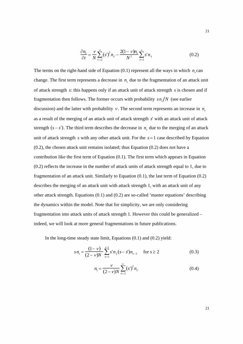
The terms on the right-hand side of Equation (0.1) represent all the ways in which ns can

change. The first term represents a decrease in ns due to the fragmentation of an attack unit

of attack strength s: this happens only if an attack unit of attack strength s is chosen and if

fragmentation then follows. The former occurs with probability sns N (see earlier

discussion) and the latter with probability ν . The second term represents an increase in ns

as a result of the merging of an attack unit of attack strength s' with an attack unit of attack

strength s − s'( ). The third term describes the decrease in ns due to the merging of an attack

unit of attack strength s with any other attack unit. For the s =1 case described by Equation

(0.2), the chosen attack unit remains isolated; thus Equation (0.2) does not have a

contribution like the first term of Equation (0.1). The first term which appears in Equation

(0.2) reflects the increase in the number of attack units of attack strength equal to 1, due to

fragmentation of an attack unit. Similarly to Equation (0.1), the last term of Equation (0.2)

describes the merging of an attack unit with attack strength 1, with an attack unit of any

other attack strength. Equations (0.1) and (0.2) are so-called ‘master equations’ describing

the dynamics within the model. Note that for simplicity, we are only considering

fragmentation into attack units of attack strength 1. However this could be generalized –

indeed, we will look at more general fragmentations in future publications.

In the long-time steady state limit, Equations (0.1) and (0.2) yield:

sns =1− ν( )

2 − ν( )N s'ns' s− s'( )ns− s's'=1

s−1

∑ for s ≥ 2 (0.3)

n1 =ν

2 −ν( )Ns'( )2 ns'

s'= 2

∞

∑ (0.4)

22

22

Equations of this type are most conveniently treated using the general technique of

‘generating functions’. As the name suggests, these are functions which can be used to

generate a range of useful quantities. Consider

G y[ ]= s' ns' ys'

s'= 0

∞

∑ (0.5)

where y = e−ω is a parameter. Note that sns N is the probability of finding an attack unit

of attack strength s. If G y[ ] is known, sns is then formally given by

sns =1s!

G(s) 0[ ] (0.6)

where G(s) y[ ] is the s-th derivative of G y[ ]with respect to y . G(s) y[ ] can be decomposed

as

G y[ ]= n1 y + s'ns's'= 2

∞

∑ y s' ≡ n1 y + g y[ ] (0.7)

where the function g y[ ] governs the attack-units’ attack-strength distribution ns for s ≥ 2.

The next task is to obtain an equation for g y[ ]. This can be done in two ways. One could

either write down the terms in g y[ ]( )2 explicitly and then make use of Equation (0.3), or

one could construct g y[ ] by multiplying Equation (0.3) by e−ωs and then summing over s.

The resulting equation is:

g y[ ]( )2−

2 −ν1−ν

N − 2n1 y⎛ ⎝

⎞ ⎠ g y[ ]+ n1

2 y 2 = 0 (0.8)

First we solve for n1. From Equation (0.7), g 1[ ]= G 1[ ]− n1 = N − n1. Substituting

n1 = N − g 1[ ] into Equation (0.8) and setting y = 1, yields

g 1[ ]=1− ν2 − ν

N (0.9)

Hence n1 = N − g 1[ ]=1

2 − νN (0.10)

23

23

To obtain ns with s ≥ 2, we need to solve for g y[ ]. Substituting Equation (0.10) for n1,

Equation (0.8) becomes

g y[ ]( )2−

2 −ν1−ν

N −2N

2 − νy⎛

⎝ ⎞ ⎠ g y[ ]+

N 2

2 −ν( )2 y 2 = 0 (0.11)

Equation (0.11) is a quadratic equation for g y[ ] which can be solved to obtain

g y[ ]=2 − ν( )N4 1−ν( )

1− 1−4 1− ν( )2 − ν( )2 y

⎛

⎝ ⎜

⎞

⎠ ⎟

2

=2 − ν( )N4 1−ν( )

2 −4 1−ν( )2 − ν( )2 y − 2 1−

4 1− ν( )2 − ν( )2 y

⎛

⎝ ⎜

⎞

⎠ ⎟ .

(0.12)

Using the expansionvi

1− x( )1 2 =1−12

x −(2k − 3)!!

(2k)!!k = 2

∞

∑ x k , (0.13)

we have

g y[ ]=2 − ν( )N2 1− ν( )

2k − 3( )!!2k( )!!k =2

∞

∑ 4 1−ν( )2 −ν( )2 y

⎛

⎝ ⎜ ⎞

⎠ ⎟

k

. (0.14)

Comparing the coefficients in Equation (0.14) with the definition of g y[ ] in Equation (0.7),

the probability of finding an attack unit of attack strength s is given by:

sns

N=

2 − ν( )2 1− ν( )

2s − 3( )!!2s( )!!

4 1−ν( )2 −ν( )2

⎛

⎝ ⎜ ⎞

⎠ ⎟

s

. (0.15)

It hence follows that the average number of attack units of attack strength s is

vi The ‘double factorial’ operator !! denotes the product: ( )( )!! 2 4n n n n= − − K

24

24

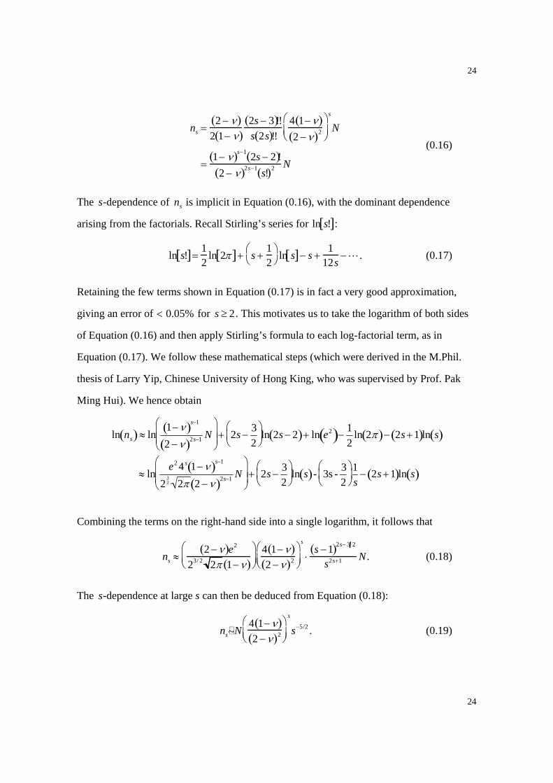
ns =

2 − ν( )2 1− ν( )

2s − 3( )!!s 2s( )!!

4 1−ν( )2 −ν( )2

⎛

⎝ ⎜ ⎞

⎠ ⎟

s

N

=1− ν( )s−1 2s − 2( )!

2 − ν( )2s−1 s!( )2 N

(0.16)

The s-dependence of ns is implicit in Equation (0.16), with the dominant dependence

arising from the factorials. Recall Stirling’s series for ln s![ ]:

ln s![ ]=

12

ln 2π[ ]+ s +12

⎛ ⎝

⎞ ⎠ ln s[ ]− s +

112s

−L . (0.17)

Retaining the few terms shown in Equation (0.17) is in fact a very good approximation,

giving an error of < 0.05% for s ≥ 2. This motivates us to take the logarithm of both sides

of Equation (0.16) and then apply Stirling’s formula to each log-factorial term, as in

Equation (0.17). We follow these mathematical steps (which were derived in the M.Phil.

thesis of Larry Yip, Chinese University of Hong King, who was supervised by Prof. Pak

Ming Hui). We hence obtain

ln ns( ) ≈ ln1−ν( )s−1

2 −ν( )2s−1 N⎛

⎝ ⎜ ⎜

⎞

⎠ ⎟ ⎟ + 2s −

32

⎛ ⎝ ⎜

⎞ ⎠ ⎟ ln 2s − 2( )+ ln e2( )−

12

ln 2π( )− 2s +1( )ln s( )

≈ lne2 4 s 1−ν( )s−1

232 2π 2 −ν( )2s−1 N

⎛

⎝ ⎜ ⎜

⎞

⎠ ⎟ ⎟ + 2s − 3

2⎛ ⎝ ⎜

⎞ ⎠ ⎟ ln s( )- 3s - 3

2⎛ ⎝ ⎜

⎞ ⎠ ⎟

1s

− 2s +1( )ln s( )

Combining the terms on the right-hand side into a single logarithm, it follows that

ns ≈2 −ν( )e2

23/ 2 2π 1−ν( )⎛

⎝ ⎜ ⎞

⎠ ⎟ 4 1−ν( )2 −ν( )2

⎛

⎝ ⎜ ⎞

⎠ ⎟

s

⋅s −1( )2s− 3 2

s2s+1 N . (0.18)

The s-dependence at large s can then be deduced from Equation (0.18):

ns N

4 1−ν( )2 −ν( )2

⎛

⎝ ⎜ ⎞

⎠ ⎟

s

s−5/2 . (0.19) ~

25

25

For small values of ν , the dominant dependence on s is therefore

ns ~ s−5 2 hence ns ~ s−2.5 (0.20)

We have therefore shown analytically that the distribution of attack strengths will follow a

power-law with a coefficient 2.5 (i.e. 5/2). As discussed earlier, we assume that any

particular attack unit could be involved in an event in a given time interval, with a

probability p which is independent of its attack size. Hence these power-law results which

we have derived for the distribution of attack strengths, will also apply to the distribution of

attacks of severity x. (Recall that the attack strength s is a measure of the number of

casualties in a typical event, and that the severity x of an event is measured as the number

of casualties). In other words, the same power-law exponent 2.5 derived in Eq. (0.20), will

also apply to the distribution of attacks having severity x.

Hence our model predicts that any guerilla-like war which is characterized by an

ongoing process of coalescence and fragmentation of attack units, and hence an

ongoing re-distribution of the total attack strength, will have the following properties:

(i) The distribution of events with severity x will follow a power-law. This finding is

consistent with the behaviour observed for the aggregated data in the Iraq and

Colombia wars (see Figure 1 of the paper).

(ii) The power-law distribution will, in the steady-state (i.e. long-time) limit, have a

coefficient of 2.5. This is precisely the value to which the results for Colombia and

Iraq currently seem to be heading (see Figure 2 of the paper).

26

26

In the case of the Iraq war, we can go one step further by providing a simple

generalization of the above model in order to offer an explanation for the evolution of the

power-law coefficient throughout the war’s entire history (recall Figure 2 of paper). The

above model is characterized by the probability ν together with the mechanism for attack-

unit coagulation and fragmentation. This value ν was chosen to be independent of the

attack strength of the individual attack units involved. In this modification, we will keep the

essential structure of the model, but we will add the modification that an attack unit will

fragment with a probability which depends on its attack strength, and will coalesce with

another attack unit with a probability depending on the attack strengths of the two attack

units involved. With probability ν the randomly-chosen attack unit i (chosen with

probability proportional to the attack strength) will fragment into attack units of attack

strength 1, with a probability f si[ ] which depends on si . With probability (1−ν) the attack

unit of attack strength si coalesces with another randomly-chosen attack unit j having

attack strength sj , with probability f si[ ]f sj[ ]. They remain separated otherwise. With the

choice f s[ ]=1 the original model is recovered. Analytically, this particular formulation of

the fragmentation and coagulation process can be readily treated by the generating function

approach discussed earlier, as will be demonstrated below.

Before proceeding, we discuss why this probabilistic ‘attack-unit-formation’ process

may indeed mimic certain aspects of guerilla warfare. One such aspect is the effect of the

arrival of opposing troops in the area. Imagine that at a given timestep and with a given

probability ν , the opposing army arrives in the vicinity of a given attack unit of attack

strength si . If the overall conflict is such that the opposing army has the

guerrillas/insurgents on the run, then this might suggest to the members of the insurgent

attack unit that they should separate and move away from the area. However, if the state of

the conflict is such that the guerilla/insurgent force feels powerful, they are unlikely to just

27

27

disband and run if they have a significant attack strength. Instead they will possibly stand

their ground and fight. Hence their probability of fragmentation is likely to be a decreasing

function of their attack strength. By contrast, with probability 1−ν( ) , no opposing troops

arrive in the vicinity of the attack unit. With probability f si[ ] ( f s j[ ]) the attack unit i ( j )

decide to join forces. Thus, the two attack units will coalesce with probability f si[ ] f sj[ ]. Again, this need for coalescing is likely to be less if the two attack units involved already

feel powerful. Hence we would expect the probability of coalescence of the two attack units

to be a decreasing function of their attack strengths. It is therefore quite plausible that --

depending on the state of the war from the insurgent force’s perspective -- the probabilities of fragmentation and coalescence should depend on f si[ ] ( f s j[ ]), i.e. they depend on the

attack strengths of the attack units involved.

Analytically, the master equations for the specific example case in which f s[ ] ~ s−δ

can readily be written down:

∂ns

∂t= −

ν s1−δ ns

N+

1− ν( )N 2 s'( )1−δ ns' (s− s')1−δ ns− s' −

2 1−ν( )s1−δ ns

N 2 s'( )1−δ ns's'=1

∞

∑s'=1

s−1

∑ for s ≥ 2 (0.21)

∂n1

∂t=

νN

s'( )2−δ ns' −2 1−ν( )n1

N 2 s'( )1−δ ns's'=1

∞

∑s'=2

∞

∑ (0.22)

with the physical meaning of each term being similar to that for Equations (0.1) and (0.2).

The steady state equations become

s1−δ ns = A s'( )1−δ ns' (s − s')1−δ ns−s's'=1

s−1

∑ (0.23)

n1 = B s'( )2−δ

s'= 2

∞

∑ ns' (0.24)

The constant coefficients A and B are given by

28

28

A =1−ν

N ν + 2 1− ν( ) s'( )1−δ ns's'=1

∞∑ and B =

N ν2 1− ν( ) s'( )1−δ ns's'=1

∞∑

Setting δ = 0 in Equations (0.23) and (0.24) recovers Equations (0.3) and (0.4) for the

original model. A generating function

G y[ ]= s'( )1−δ

s'= 0

∞

∑ ns' ys' = n1 y + g y[ ] (0.25)

can be introduced where g y[ ]= s'( )1−δ ns's'=2

∞

∑ y s' and y = e−ω . The function g y[ ] satisfies a

quadratic equation of the form

g y[ ]( )2−

1A

− 2n1 y⎛ ⎝

⎞ ⎠ g y[ ]+ n1

2 y 2 = 0 (0.26)

which is a generalization of Equation (0.8). Using n1 + g 1[ ]= s'( )1−δ

s'=1

∞∑ ns' and Equation

(0.26), n1can be obtained as

n1 =1−ν( )2 − ν2 A2 N 2

4 1−ν( )2 A (0.27)

Solving Equation (0.26) for g y[ ]gives

g y[ ]=1

4A1− 1− 4n1 A y( )2

(0.28)

Following the steps leading to Equation (0.19), we obtain ns in the modified model:

ns N

4 1−ν( ) 1− ν( )+N ν

s'( )1−δ ns's'=1

∞∑⎛

⎝ ⎜ ⎜

⎞

⎠ ⎟ ⎟

N νs'( )1−δ ns's'=1

∞

∑+ 2 1−ν( )

⎛

⎝ ⎜ ⎜

⎞

⎠ ⎟ ⎟

2

⎛

⎝

⎜ ⎜ ⎜ ⎜ ⎜ ⎜

⎞

⎠

⎟ ⎟ ⎟ ⎟ ⎟ ⎟

s

s−(5/2−δ ) (0.29)

For δ = 0, s'( )1−δ

s'=1

∞∑ ns' = N and hence Equation (0.29) reduces to the result in Equation

(0.19) for the original model. Forδ ≠ 0, it is difficult to solve explicitly for ns . However the

~

29

29

summation simply gives a constant, and thus for small ν the dominant dependence on the

attack strength s is ns ~ s− 5 2−δ( ) and hence equivalently ns ~ s− 2.5−δ( ).

Most importantly, we can see that by decreasing δ from 0.7 → 0 (i.e. by

increasing the relative fragmentation/coalescence rates of larger attack units) we span

the entire spectrum of power-law exponents observed in the Iraq war from the initial

value of 1.8, up to the current tendency towards 2.5. This effect of decreasing δ from

0.7 → 0 corresponds in our model to a relative increase in the tendency for larger

attack units to either fragment or coalesce at each timestep. In other words,

decreasing δ mimics the effect of decreasing the relative robustness or ‘lifetime’ of

larger attack units.

Going further, we note that these theoretical results are consistent with, and to some

extent explain, the various power-law exponents found for:

(1) Conventional wars. The corresponding power-law exponent 1.8 can now be interpreted

through our generalized model with δ ≈ 0.7, as a tendency toward building larger, robust

attack units with a fixed attack strength as in a conventional army -- as opposed to attack

units with rapidly fluctuating attack strengths as a result of frequent fragmentation and

coalescence processes. There is also a tendency to form a distribution of attack units with a

wide spectrum of attack strengths – this is again consistent with the composition of

‘conventional’ armies from the past.

(2) Terrorism in G7 countries. The corresponding power-law exponent 1.7 can be

interpreted through our generalized model with δ ≈ 0.8, as an even stronger tendency for

robust units (e.g. terrorist cells) to form. There is also an increased tendency to form larger

units – or rather, to operate as part of a large organization.

30

30

(3) Terrorism in non-G7 countries. The corresponding power-law exponent 2.5 can be

interpreted through our model with δ = 0, as a tendency toward more transient attack units

(e.g. terrorist cells) whose attack strengths are continually evolving dynamically as a result

of an on-going fragmentation and coalescence process. Unlike a conventional army, there

will be a tendency to form smaller attack units rather than larger ones.

Interestingly, we can now discuss the evolution of the wars in Colombia and Iraq in these

terms:

War in Colombia. At the beginning of the 1990’s, the power-law exponent was very high

(3.5). Then over the following 15 years, it gradually lowered to the present value and

appears to be tending toward 2.5. Using our model, the interpretation is that the war at the

beginning of the 1990’s was such that the guerrillas favoured having small attack units.

This is possibly because they lacked communications infrastructure, and/or did not feel any

safety in larger numbers. The decrease toward the value 2.5, suggests that this has changed

– probably because of increased infrastructure and communications, enabling attack units

with a wide range of attack strengths to build up.

War in Iraq. At the beginning of the war in 2002, the power-law exponent was quite low

(1.8) and was essentially the same value as conventional wars. This is consistent with the

war being fought by a conventional Iraqi army against the Coalition forces. There is then a

break in this value after a few months (i.e. the war ended) and following this, the power-

law exponent gradually rises towards 2.5. This suggests that the insurgents have been

increasingly favouring more temporary attack units, with an increasingly rapid

fragmentation-coalescence process. This finding could be interpreted as being a result of

31

31

increased success by the Coalition Forces in terms of forcing the insurgents to fragment. On

the other hand, it also means that the Iraq War has now moved to a value, and hence

character, which is consistent with generic non-G7 terrorism.

32

32

PART 2: Supplementary tables and figures which help confirm the robustness of our

results

Estimates of power-law coefficients for the entire time-series

1α Confidence

Interval

Percentage of

points inside

interval

2α Confidence

Interval

Adjusted R2

K 3.1013 +/- 0.02 0.95% 2.8761 +/- 0.0151 0.9835

I 3.04 +/- 0.02 0.95% 2.9717 +/- 0.0211 0.9818

KI 2.93 +/- 0.015 0.95% 3.0061 +/- 0.0179 0.9796

CKmin 2.07 +/- 0.005 0.90% 2.1279 +/- 0.0057 0.9336

CKmax 2.02 +/- 0.003 0.90% 2.0966 +/- 0.0043 0.9496

Supplementary Table 1 Shows two complementary estimates of the power-law

coefficients for the variables K (reported deaths for Colombia), I (reported injuries

for Colombia), KI (reported deaths plus injuries for Colombia), CKmin (minimum

reported civilian deaths for Iraq) and CKmax (maximum reported civilian deaths for

Iraq). Our first estimate ( 1α ) uses α =1+ n ln xixmin

⎛ ⎝ ⎜ ⎞

⎠ ⎟

i=1

n

∑⎡

⎣ ⎢

⎤

⎦ ⎥

−1

while our second

estimate ( 2α ) uses ordinary least-squares linear regression. The two results are

always very similar and the results vary little as we vary the victimization measure

for Colombia. For further discussion, see PART 3 of this Supplementary

Information document.

33

33

Supplementary Figure 2 The variation through time of the power law coefficients

for three 2,500 day intervals displaced by 1,855 days for the Colombian data and

three 365 day intervals displaced every 258 days for the Iraq data. Despite this

change in size of the windows and how they slide across time both curves seem to

be tending toward 2.5, as in Figure 2 of the paper. For further discussion, see

PART 3 of this Supplementary Information document.

34

34

Supplementary Figure 3 The variation through time of the power law coefficients

for two year intervals displaced every year for Colombia and 200 day intervals

displaced every 200 days for Iraq. Again, they both seem to be tending toward 2.5,

as in Figure 2 of the paper. For further discussion, see PART 3 of this

Supplementary Information document.

35

35

Supplementary Figure 4 Log-Log plots of cumulative distributions )( xXP ≥

describing events greater than x , for the minimum possible value and maximum

possible value of each event in the Iraq dataset. The results are very much the

same across the two measures. For further discussion, see PART 3 of this

Supplementary Information document.

36

36

PART 3: Supplementary Notes on Methods

If α−= Cxxp )( , then, )1(min)1( −−= αα xC and α =1+ n ln xi

xmin

⎛

⎝ ⎜

⎞

⎠ ⎟

i=1

n

∑⎡

⎣ ⎢

⎤

⎦ ⎥

−1

.

We used two estimates for α (see Supplementary Information Table 1 in PART 2). We

estimated 1α using α with minx equal to the minimum value that satisfies the Kolmogorov

statistic for the whole data set. We estimated 2α using ordinary least-square regression

analysis for all the values greater than minx .

We established minx as the minimum value of x where we could not reject the

hypothesis that the data beyond minx followed a power law using a Kolmogorov-Smirnov

goodness of fit test at 95% confidence.

In order to estimate the error of α , we used a minus-one jackknife resampling

method. We created the datasets obtained by removing one value from the original dataset.

For each of these surrogates, we estimated α and C . We then measured the maximum and

minimum deviation from the mean of the parameters α obtained from the diverse

jackknife datasets. We established an interval equal to the maximum distance from the

mean of the sample times 5. Since this is not an analytical solution, we present the

percentage of values that fall into that interval.

The Evolution of α : To test the robustness of our findings in Figure 2 of the paper, we

have repeated the calculation of α for several different sizes of the time windows. We also

tried varying the way in which these windows slide forward in time. All these changes

barely affected our results.

As an example, in Part 2 of this document we have plotted the evolution of KI (deaths

and injuries) for different time windows. For the Colombian data set we used a time

37

37

window of 2,500 days moved every 1,855 days (see Supplementary Figure 2); then a

moving time window of two years displaced every year (see Supplementary Figure 3), and

finally a moving time window of two years, displaced every 50 days (Figure 1). For the

Iraq data set we used a 365 day time window displaced every 258 days (Supplementary

Figure 2), a 250 day interval displaced every 150 days (Supplementary Figure 3), and a 365

day time window displaced every 30 days (Figure 1). As can be seen, our results are

essentially unchanged by these variations.

Further general comment on robustness testing: As a further test of the robustness of

the results obtained in our paper, and in particular our main findings in Figures 1 and 2 of

the paper, we ran the following variations of our calculations. For Colombia we used just

killings and just injuries, rather than killings plus injuries as presented in the paper. For

Iraq we used the maximum number of deaths rather than the minimum number of deaths as

reported in the paper. These results are shown in Supplementary Figure 4. As can be seen,

these variations do not affect our findings. This is reassuring, and is actually not too

surprising since the power-law coefficient α provides a statistical measure of the structure

of the events’ time-series, rather than the absolute number of killings and/or injuries. Hence

the power-law coefficient α will be unaffected by any constant scale factors which are

introduced as a result of a fixed ratio of injuries to killings.

An additional, but perhaps even more important, advantage of focusing on α ,

concerns possible over- or under-reporting of war casualties. In particular, α is insensitive

to systematic over-reporting or under-reporting of casualties. This is because any

systematic multiplication of the raw numbers by some constant factor, has no affect on the

α value which emerges from the log-log plot.