from occurrence to eco-evolutionary dynamicshss.ulb.uni-bonn.de/2016/4381/4381.pdf ·...
TRANSCRIPT
Dissertation by Jan O. Engler
From occurrence to
Assessing connectivity in a changing world through modelling and landscape genetics
eco-evolutionary dynamics
FROM OCCURRENCE TO ECO-EVOLUTIONARY
DYNAMICS: ASSESSING CONNECTIVITY IN A
CHANGING WORLD THROUGH MODELING AND
LANDSCAPE GENETICS
Dissertation
zur Erlangung des Doktorgrades (Dr. rer. nat.)
der
Mathematisch-Naturwissenschaftlichen Fakultät
der
Rheinischen Friedrich-Wilhelms-Universität Bonn
vorgelegt von
Jan Oliver Engler
aus
Oberhausen
Bonn, November 2015

THESIS COMMITTEE Prof. Dr. J. WOLFGANG WÄGELE (Erstgutachter)Director ZFMK Zoological Research Museum Alexander Koenig
Prof. Dr. BERNHARD MISOF (Zweitgutachter)Director ZMB Zoological Research Museum Alexander Koenig
Prof. Dr. NIKO BALKENHOL (Fachnahes Mitglied)Head of Department of Wildlife Sciences Büsgen Institut, University of Göttingen
Prof. Dr. GABRIELE M. KÖNIG (Fachfernes Mitglied)Professor of Pharmaceutical Biology Institute of Pharmaceutical Biology, University of Bonn

Angefertigt mit Genemigung der Mathematisch-Naturwissenschaftlichen Fakultät der Rheinischen Friedrich-Wilhelms-Universität Bonn.
Die Arbeit wurde am Zoologischen Forschungsmuseum Alexander Koenig in Bonn durchgeführt
Tag der mündlichen Prüfung: 25.05.2016


Erklärung
Hiermit versichere ich, Jan O. Engler, dass ich diese Arbeit selbständig verfasst, keine
anderen Quellen und Hilfsmittel als die angegebenen verwendet, und die Stellen der Arbeit,
die anderen Werken dem Wortlaut oder dem Sinn nach entnommen sind, unter Angabe der
Quelle kenntlich gemacht habe. Ich versichere außerdem, dass ich die beigefügte Dissertation
nur in diesem und keinem anderen Promotionsverfahren eingereicht habe und, dass diesem
Promotionsverfahren keine endgültig gescheiterten Promotionsverfahren vorausgegangen
sind.
Bonn, den 18.11.2015


Jan O. Engler
From occurrence to eco-evolutionary dynamics: assessing connectivity in a changing world through modeling and landscape genetics
Date of defense: 25.05.2016
Thesis, University of Bonn, Bonn, Germany (2016)
With references, with summaries in Englisch and German

Contents
List of Figures
List of Tables
Aims & Scope 1
Chapter 1: General Introduction 7
What is connectivity? 9
Connectivity in Conservation and Environmental Planning 11
Connectivity in Landscape Genetics 13
Chapter 2: Conception of Potential Connectivity Models 17
Environmental Information 19
Occurrence Information 21
The SDM 21
The Connectivity Model 23
Linking genetic information with PCMs 23
PART A – PCM’S IN CONSERVATION & ENVIRONMENTALPLANNING 27
Chapter 3: Accounting for the ‘network’ in the Natura 2000 network: A response to Hochkirch et al. 2013 29
Commentary 31
Chapter 4: Missing the target? A critical view on butterfly conservation efforts on calcareous grasslands in south-western Germany 35
Introduction 37
Material and methods 39 Study sites 39
Field sampling design 41
Classification of butterfly species 42
Statistical analysis 45
Resistance surface modeling 46
Results 49 Species decline 49
Degradation of functional groups 50
Changes in relative trait diversity 51
Connectivity modeling 52
Discussion 53
Chapter 5: Coupling satellite data with species distribution and connectivity models as a tool for environmental management and planning in matrix-sensitive species 59
Introduction 61
Material and methods 65 Study area and data sampling 65
Satellite data 67
Potential Connectivity Model 68
Results 72 Estimated condition status of Colognes’ sand lizard populations basedon field
observations 72
Distribution of potential habitats 72
Predicted connectivity between populations 73
Discussion 74 Applicability of the approach 74
Data requirements and limitation for further applications 78
Conclusion 79
PART B – PCM’S IN LANDSCAPE GENETICS 83
Chapter 6: Comparative landscape genetics of three closely related sympatric Hesperid butterflies with diverging ecological traits 85
Introduction 87
Material and methods 89 Ethics statement 89
Study area and species 89
Molecular data and genetic cluster analysis 90
Modelling landscape effects on genetic differentiation 92
Comparing connectivity estimates with genetic data 95
Results 96 Genetic structures 96
Genetic clustering results 97
Species Distribution Models 97
Landscape effects of genetic differentiation 98
Discussion 102 Diverging responses to identical landscape conditions 103
Accounting for FST and Dest in landscape genetic studies 106
Conclusion 107
Supplementary material 109
Chapter 7: A statistical learning approach to improve ecological inferences in landscape genetics by accounting for spatial nonstationarity of genetic differentiation 117
Introduction 119
Material and methods 122 The statistical learning approach 122
Empirical examples 123
Results 125
Discussion 126
Supplementary material 131
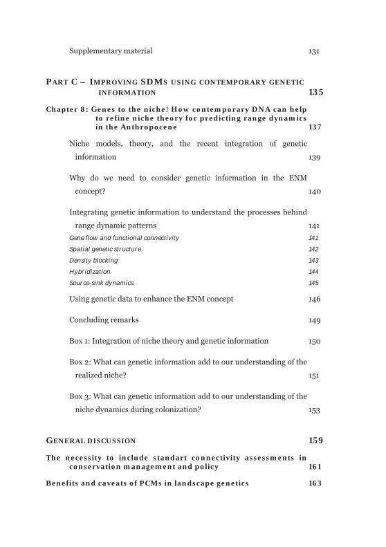
PART C – IMPROVING SDMS USING CONTEMPORARY GENETIC INFORMATION 135
Chapter 8: Genes to the niche! How contemporary DNA can help to refine niche theory for predicting range dynamics in the Anthropocene 137
Niche models, theory, and the recent integration of genetic
information 139
Why do we need to consider genetic information in the ENM
concept? 140
Integrating genetic information to understand the processes behind
range dynamic patterns 141 Gene flow and functional connectivity 141
Spatial genetic structure 142
Density blocking 143
Hybridization 144
Source-sink dynamics 145
Using genetic data to enhance the ENM concept 146
Concluding remarks 149
Box 1: Integration of niche theory and genetic information 150
Box 2: What can genetic information add to our understanding of the
realized niche? 151
Box 3: What can genetic information add to our understanding of the
niche dynamics during colonization? 153
GENERAL DISCUSSION 159
The necessity to include standart connectivity assessments in conservation management and policy 161
Benefits and caveats of PCMs in landscape genetics 163

From genes to ranges and back: is niche theory ready for the Anthropocene? 166
Personal outlook 167
SUMMARIES 169
Summary 171
Zusammenfassung 175
ACKNOWLEDGEMENTS 181
REFERENCES 187
CURRICULUM VITAE 225

List of Figures
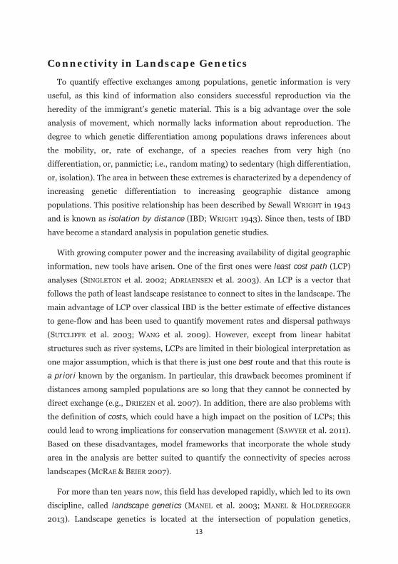
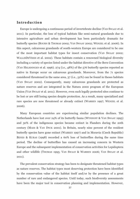
Figure 1.1: Illustration of the differences between structural connectivity and functional connectivity for mobile and matrix-sensitive species 10
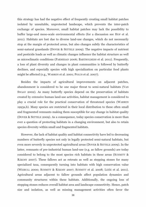
Figure 2.1: The potential connectivity model (PCM) framework 19
Figure 4.1: Location of the study area near Trier in south-western Germany as well as habitat suitability and potential connectivity maps from the same region. 53
Figure 4.2: Trait space spanned by the first two principal components for either vineyard fallows and calcareous grasslands. 54
Figure 5.1: Two-step conceptional framework for performing potential connectivity models. 64
Figure 5.2: Potential distribution and connectivity of the sand lizard in the city of Cologne. 76
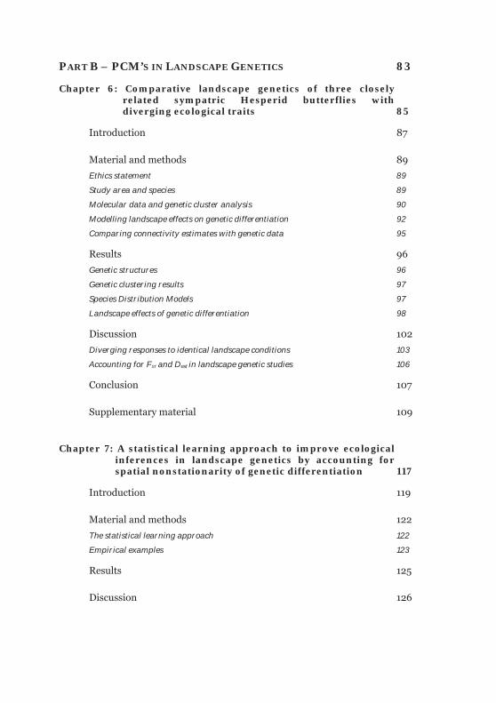
Figure 6.1: Locations of populations studied for all three Thymelicus species in southwestern Germany and adjoining areas in France and Luxemburg. 92
Figure 6.2: SDM output for Thymelicus lineola and T. sylvestris as well as T. acteon. 98
Figure 6.3: Schematic illustration about the gradual effects forcing the three Thymelicus species. 102
Material 6.S1 Figure 1: Consensus tree inferred by using the Neighbor-Joining method accounting for the 50% majority rule. 110
Figure 6.S1: Estimation of the number of panmictic clusters for each species. 113
Figure 6.S2: Scatterplots showing the difference of isolation by distance patterns with isolation by resistance patterns in the two species that show a spatial genetic structure. 114
Figure 7.1: A fictive study area that comprises seven localities where genetic information from a species was obtained but where relationships to landscape elements are unknown. 121
Figure 7.2: Spatial composition of regions where one of the three landscape elements is locally driving gene flow in the study region. 122
Figure 7.3: Linear relationships between genetic distance with effective distances from land use, topography, and climate together with the optimized solution for the Hesperid butterfly Thymelicus sylvestris. 126
Figure 7.4: The optimized solution plotted as a network of comparisons across the study area from T. sylvestris. 127
Figure 7.5: Linear relationships between genetic distance with effective distances from range shape and climate together with the optimized for the wolverine. 128
Figure 7.6: The optimized solution plotted as a network of comparisons across the North American range of the wolverine. 129
Figure 8.1: The fraction of the BAM plot where species occur. 140
Figure 8.2: Expanding the ENM concept with genetic information. 147
Figure 8.B1.1: The BAM diagram as an abstract visualization of the ENM concept in geographic space. Biological and ecological aspects than can be quantified with genetic information can be linked to certain compartmentd of this concept. 150
Figure 8.B2.1: Integrating information on contemporary gene flow into niche modeling and theory. 151
Figure 8.B2.2: Accounting for spatial genetic structure in niche modeling. 152
Figure 8.B3.1: Two examples of biological invasions where density blocking may play a key role are Rubus alceifolius and Ambrosia artemisiifolia. 153
Figure 8.B3.2: Invasion success due to increased adaptive potential following hybridization may result in different niche dynamics. 155
List of Tables
Table 4.1: Presence-absence data of all butterfly species recorded. 43
Table 4.2: Factor loadings as well as Eigenvalues and cumulative explained variance for each of the three Principal components extracted. 52
Table 4.3: Percentage of the importance of predictor variables used for constructing environmental niche models. 56
Table 5.1: Details of the spectral bands covered by Landsat and indices calculated based upon them. 68
Table 5.2: Condition status of the investigated sand lizard populations in Cologne in 2011. 73
Table 5.3: Variable importance as measured with three different procedures in Maxent. 77
Table 6.1: Summary statistics for genetic diversity and differentiation for the three Thymelicus butterflies. 96
Table 6.2: Comparison of the genetic structure in three Thymelicus butterflies with different landscape parameter sets. 100
Table 6.3: Averaged variable contributions for the scenarios ‘topography’, ‘climare’ and ‘all’. 103
Table 6.S1: Geographic coordinates of the sampling locations. 109
Material 6.S1 Table 1: Species and GenBank accession numbers of the individuals used for estimating genetic distance between species. 111
Material 6.S1 Table 2: Uncorrected pairwise genetic distance of the COI sequences within and between species of the genus Thymelicus 111
Table 6.S2: Description of the landscape data used for resistance surface building depending on the scenario assumed. 112
Table 7.S1: Predictors used for conducting the SDM for the wolverine. 132

1
AIMS & SCOPE
“A journey of a thousand miles begins with a single step. Dissertations begin with a single word.”
ALESHIA TAYLOR HAYES AS MODIFIED FROM LAOZI

2
3
Aims & Scope
Climate change and the intensification of human landuse are generally accepted as
leading factors for global biodiversity loss (BELLARD et al. 2012; DEVICTOR et al. 2012).
However, considering both factors in synergy, the effect of species loss could be even
higher (TRAVIS 2003; HOF et al. 2011) and go way beyond what we expected from
climate change alone (PARMESAN & YOHE 2003; THOMAS et al. 2004).
Habitat loss and fragmentation can hamper the exchange among populations or
even prevent it. This can lead to negative demographic and genetic effects for the
affected populations (TEMPLETON et al. 1990; KEYGHOBADI 2007). These effects,
imprinted in genes, range from a decrease of genetic diversity (e.g., HABEL & SCHMITT
2012) and inbreeding (ANDERSEN et al. 2004; ZACHOS et al. 2007), up to the
extinction of affected populations (PETTERSON 1985).
To counteract these effects, and to develop more efficient conservation efforts,
knowledge on population connectivity is mandatory. This thesis aims to contribute to
this knowledge by linking tools from different disciplines for their application in
conservation planning and spatial ecology. Known as potential connectivity models
(PCMs), they will cover two main parts of the thesis:
Part A: Generating additional information about fine scale and spatially explicit
exchanges in matrix sensitive species for conservation management and environmental
planning.
Part B: Quantifying landscape elements responsible for the genetic exchange among
populations across spatial scales using contemporary genetic information.
The methodological concept behind PCMs is identical for both parts, but makes
additional use of genetic information for the quantification of connectivity in Part B.
A central part of PCMs are predictive niche models (also known as species
distribution models—SDMs—or environmental niche models—ENMs). Thanks to the
increasing availability of digital spatial data, SDMs became a central tool in the
analysis of species distributions over the past decade (FRANKLIN 2009). SDMs were
4
used in a lot of ecological and evolutionary disciplines, covering a broad range of
spatial and temporal scales and have been central to a lot of conservation-related
aspects such as reserve design and species action plans (GUISAN et al. 2013).
Aside from all the opportunities that SDMs can offer to the scientific community,
there are a lot of conceptual and methodological challenges to face. Methodological
and technical errors can result in poor models and their predictions could lead to
wrong implications e.g. for conservation management. Based on this, potential error
sources such as the choice of environmental predictors, the most suitable algorithm,
or the impact of gaps in species occurrence information, are part of an ongoing
discussion in the scientific community (e.g., GUISAN & ZIMMERMANN 2000;
HERNANDEZ et al. 2006; WISZ et al. 2008; VAN GILS et al. 2014). One core problem is
that the available methods to estimate model fit are dependent on the contrast
between the environmental conditions at the occurrence location by those from a
chosen background area (or true absence records). This way of evaluation, however,
is prone to systematic errors due to over-parameterization when using predictors that
are too heterogeneous, or too many predictors at all (e.g., GUISAN & ZIMMERMAN
2000; DORMANN et al. 2007). Detected contrasts are then no longer biological signals,
but statistical artifacts. From this, a general question is derived: how much biological
relevance is covered in a statistically good SDM? What can such a model tell us about
the biological requirements for a species to persist within its populations and
successfully exchange among them? An independent measure of high biological
relevance could shed light into these issues. In this regard, the third part of this thesis
is:
Part C: How can contemporary genetic information inform SDMs to generate better
predictions for current and future ranges in a changing world?
In this section, the framework from Part A & B is not used to gain ecological
insight about the functional connectivity of a species. Instead, ecological principles
(e.g., functional connectivity) that can be assessed using genetic information (e.g.,
gene-flow) are used here to inform SDMs and evaluate their fit from a biological
perspective.
5
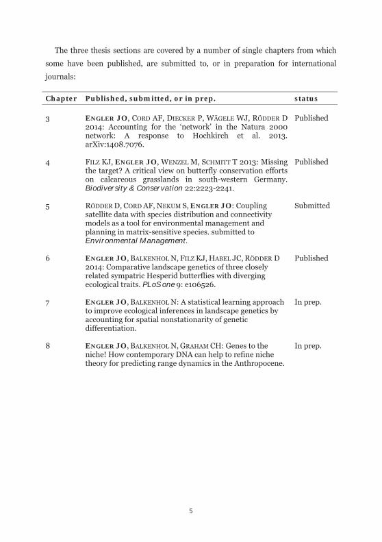
The three thesis sections are covered by a number of single chapters from which
some have been published, are submitted to, or in preparation for international
journals:
Chapter Published, submitted, or in prep. status 3 ENGLER JO, CORD AF, DIECKER P, WÄGELE WJ, RÖDDER D
2014: Accounting for the ‘network’ in the Natura 2000 network: A response to Hochkirch et al. 2013. arXiv:1408.7076.
Published
4 FILZ KJ, ENGLER JO, WENZEL M, SCHMITT T 2013: Missing the target? A critical view on butterfly conservation efforts on calcareous grasslands in south-western Germany. Biodiversity & Conservation 22:2223-2241.
Published
5 RÖDDER D, CORD AF, NEKUM S, ENGLER JO: Coupling satellite data with species distribution and connectivity models as a tool for environmental management and planning in matrix-sensitive species. submitted to Environmental Management.
Submitted
6 ENGLER JO, BALKENHOL N, FILZ KJ, HABEL JC, RÖDDER D 2014: Comparative landscape genetics of three closely related sympatric Hesperid butterflies with diverging ecological traits. PLoS one 9: e106526.
Published
7 ENGLER JO, BALKENHOL N: A statistical learning approach to improve ecological inferences in landscape genetics by accounting for spatial nonstationarity of genetic differentiation.
In prep.
8 ENGLER JO, BALKENHOL N, GRAHAM CH: Genes to the niche! How contemporary DNA can help to refine niche theory for predicting range dynamics in the Anthropocene.
In prep.

6

7
CHAPTER 1
General Introduction
“When we try to pick out anything by itself, we find it hitched to everything else in the Universe.”
JOHN MUIR

8
9
What is connectivity?
Ever since the term connectivity spread within the field of biology and applied
biological conservation, questions arose about what it is exactly and how one can
characterize or quantify it. In a very broad sense, connectivity is the degree of
exchange of organisms or processes (CROOKS & SANJAYAN 2006)—the more exchange,
the more connectivity.
Up to this point, the idea of connectivity is rather reasonable. The problem starts if
we want to narrow down the definition with further detail. It then becomes obvious
that connectivity depends on the spatial and temporal scale, the study system, and
even the scientific background of the researcher. When it comes to applications, a
universal definition of connectivity is therefore impossible.
Depending on the landscape and the focal study organism, there are two broad
types of connectivity: (1) structural connectivity, which focuses on the spatial
arrangement of landscape elements no matter the demands of the species or its
mobility; and (2) functional connectivity, which focuses on the realized use of the
landscape matrix by a species. In contrast to structural connectivity, a functional
perspective always needs information about the species’ specific habitat use (BENNETT
1999; TISCHENDORF & FAHRIG 2000; TAYLOR et al. 2006).
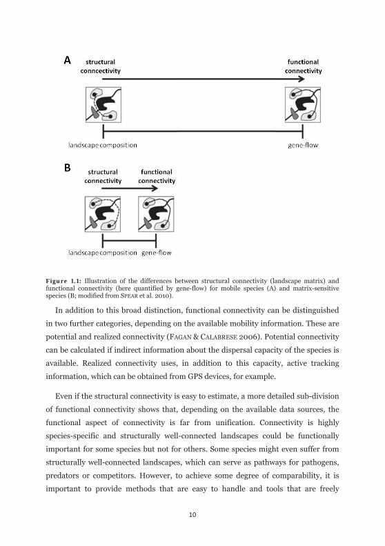
The differences between structural and functional connectivity can be rather large
or very similar (Fig. 1.1). If, for instance, a species is strongly dependent on certain
landscape elements and its movement decisions are defined by the landscape (e.g.,
lizards), then we call it a matrix-sensitive species (IMS 1995). In this case, the
structural connectivity is identical to the functional connectivity—or at least rather
similar. In contrast, mobile species (e.g., birds) are able to cross areas that are
uninhabitable for them. For these species, the differences between structural and
functional connectivity can be large.
10
Figure 1.1: Illustration of the differences between structural connectivity (landscape matrix) and functional connectivity (here quantified by gene-flow) for mobile species (A) and matrix-sensitive species (B; modified from SPEAR et al. 2010).
In addition to this broad distinction, functional connectivity can be distinguished
in two further categories, depending on the available mobility information. These are
potential and realized connectivity (FAGAN & CALABRESE 2006). Potential connectivity
can be calculated if indirect information about the dispersal capacity of the species is
available. Realized connectivity uses, in addition to this capacity, active tracking
information, which can be obtained from GPS devices, for example.
Even if the structural connectivity is easy to estimate, a more detailed sub-division
of functional connectivity shows that, depending on the available data sources, the
functional aspect of connectivity is far from unification. Connectivity is highly
species-specific and structurally well-connected landscapes could be functionally
important for some species but not for others. Some species might even suffer from
structurally well-connected landscapes, which can serve as pathways for pathogens,
predators or competitors. However, to achieve some degree of comparability, it is
important to provide methods that are easy to handle and tools that are freely

11
available so that their use is not restricted to just a few experts, but open to
stakeholders and managers, as well.
Connectivity in Conservation and Environmental Planning
In 1992, the European Union set its first directive for nature conservation. The
goal of the habitat directive (92/43/EEC) was to stop biodiversity loss within its
communal borders. The directive was the legal basis for the EU-wide reserve
network, Natura 2000, and obliges member states to conserve species and habitats
listed in Annexes II, IV and V. In addition, Art. 10 of the habitat directive calls for the
need to achieve ‘ecological coherence’ (i.e. connectivity conservation) among Natura
2000 sites (KETTUNEN et al. 2007).
In Germany, the Federal Nature Conservation Act (BNatSchG) is responsible for
the national implementation of the habitat directive. Here, Art. 21 of the BNatSchG
regulates the presets from the Art. 10 habitat directive, setting the scene for a legal,
country-wide network of habitats. Since its revision in 2006, the BNatSchG became
more restrictive, making Art 44(1) especially central here. In the following, Art. 44(1)
is printed in its original (translated) form (from
http://www.bmub.bund.de/fileadmin/Daten_BMU/Download_PDF/Naturschutz/b
natschg_en_bf.pdf, accessed at 18/08/2015):
Article 44 Provisions for specially protected fauna and flora species and other certain
fauna and flora species
(1) It is prohibited:
1. to pursue, capture, injure or kill wild animals of specially protected species, or to take
from the wild, damage or destroy their developmental stages,
2. to significantly disturb wild animals of strictly protected species and of European bird
species during their breeding, rearing, molting, hibernation and migration periods; a
disturbance shall be deemed significant if it causes the conservation status of the local
population of a species to worsen,
12
3. to take from the wild, damage or destroy breeding or resting sites of wild animals,
4. to take from the wild, wild plants of specially protected species, or their
developmental stages, or to damage or destroy them or their sites.
From this, it is clearly visible that the legal conditions for conducting
environmental impact assessments, which are the formal procedure in environmental
planning, focus mainly on the protection of source populations. In other words, even
if the habitat quality of an area is good for a focal species, it does not mean that such a
site would also be protected under Art. 44(1), unless it were known that the species is
actually present there (i.e., records on the species’ presence in that area are
available). Further, by following this law strictly, habitats that are important for
connectivity (i.e., areas of small metapopulations, through which individuals may
pass but not necessarily remain) are more likely to disappear than areas used for
reproduction (i.e., source populations with a higher density of individuals); Art. 44(1)
finds no conflict here, and thus there is no legal barrier to stop development in such
habitats.
One major problem is defining a local population, which is by no means an easy
task (see WEMDZIO 2011 and references therein). Habitats of poor quality for
reproduction in matrix-sensitive species could especially be mandatory to maintain
connectivity in neighboring populations where habitat quality is better, thereby
building up a local population. The most often flawed distinction of a local population
in environmental planning can therefore lead to a stronger fragmentation of
populations of species with a special protection status. This is a dilemma, because in
such a situation, Art. 44(1) is not immediately conflicted. However, it could cause a
time-lagged decline of the species of interest due to a loss of connectivity. This will
indeed stand in conflict with Art. 44(1), but only well after a development has been
realized. Therefore, it is mandatory to quantify potential connectivity in these species
in an objective way as an additional source of information to characterize local
populations.
13
Connectivity in Landscape Genetics
To quantify effective exchanges among populations, genetic information is very
useful, as this kind of information also considers successful reproduction via the
heredity of the immigrant’s genetic material. This is a big advantage over the sole
analysis of movement, which normally lacks information about reproduction. The
degree to which genetic differentiation among populations draws inferences about
the mobility, or, rate of exchange, of a species reaches from very high (no
differentiation, or, panmictic; i.e., random mating) to sedentary (high differentiation,
or, isolation). The area in between these extremes is characterized by a dependency of
increasing genetic differentiation to increasing geographic distance among
populations. This positive relationship has been described by Sewall WRIGHT in 1943
and is known as isolation by distance (IBD; WRIGHT 1943). Since then, tests of IBD
have become a standard analysis in population genetic studies.
With growing computer power and the increasing availability of digital geographic
information, new tools have arisen. One of the first ones were least cost path (LCP)
analyses (SINGLETON et al. 2002; ADRIAENSEN et al. 2003). An LCP is a vector that
follows the path of least landscape resistance to connect to sites in the landscape. The
main advantage of LCP over classical IBD is the better estimate of effective distances
to gene-flow and has been used to quantify movement rates and dispersal pathways
(SUTCLIFFE et al. 2003; WANG et al. 2009). However, except from linear habitat
structures such as river systems, LCPs are limited in their biological interpretation as
one major assumption, which is that there is just one best route and that this route is
a priori known by the organism. In particular, this drawback becomes prominent if
distances among sampled populations are so long that they cannot be connected by
direct exchange (e.g., DRIEZEN et al. 2007). In addition, there are also problems with
the definition of costs, which could have a high impact on the position of LCPs; this
could lead to wrong implications for conservation management (SAWYER et al. 2011).
Based on these disadvantages, model frameworks that incorporate the whole study
area in the analysis are better suited to quantify the connectivity of species across
landscapes (MCRAE & BEIER 2007).
For more than ten years now, this field has developed rapidly, which led to its own
discipline, called landscape genetics (MANEL et al. 2003; MANEL & HOLDEREGGER
2013). Landscape genetics is located at the intersection of population genetics,
14
landscape ecology and spatial statistics (STORFER et al. 2007), although some authors
argue that this field has yet to fulfill the requirements for being called
interdisciplinary (DYER 2015a). The central goal of landscape genetics is to
understand which landscape elements are responsible for gene-flow or its restriction.
For this, analyses need to go beyond IBD and LCPs. One core concept in this regard is
the quantification of genetic differentiation by estimating spatial resistances. Adapted
from IBD-theory, genetic differentiation increases with increasing spatial resistances.
In its simplest form, this spatial resistance is IBD, but it can also be restricted by
functional barriers of certain landscape elements. This concept was introduced as
isolation-by-resistance (IBR; MCRAE 2006), and plenty of different methods use it to
calculate species-specific resistance surfaces and correlate these in a separate step
with genetic differentiation (e.g., MCRAE & BEIER 2007; BRAUNISCH et al. 2010; SHIRK
et al. 2010; VAN ETTEN 2011).
The parameterization of resistance surfaces is crucial for investigating IBR, but it
is far from being standardized yet. SPEAR et al. (2010) highlighted several challenges
to be faced in the coming years to reach a comparable and standardized framework
for resistance surface parameterization. Three major points are (1) the type of
parameterization, (2) the range of resistance values of the surface and (3) the
objectivity of parameterization that should turn from expert knowledge to directly
inferred biological information (SPEAR et al. 2010). Most often, resistance surfaces
are modified depending on expert opinion to improve the functional relationship
between genetic and environmental information. Ideally, future methods should use
the available biological information on genetic structure and species-environment
relationships, process them objectively and optimize parameters without the need of
using subjective expert opinion.
SDMs could be a possible way to meet these challenges as they objectively process
ecologically-relevant information about the distribution of a species into a probability
surface of potential occurrence. The inverse probability surface could then be used as
a resistance surface for landscape genetic studies. Several studies followed this logic
and used SDMs to parameterize resistance surfaces (e.g., WANG et al. 2008; ROW et
al. 2010).
Because of their high potential, SDMs are the core of the PCM framework, as
shown in this thesis. In the following chapter, I will to provide detailed information

15
on the methodological background of the conceptual framework of PCMs, the role of
the implemented SDMs, and the data needed for analysis.

16

17
CHAPTER 2
Conception of Potential Connectivity Models
“Ecology is the art of proving the obvious with increasingly sophisticated statistics.”
KEVIN RICE

18
19
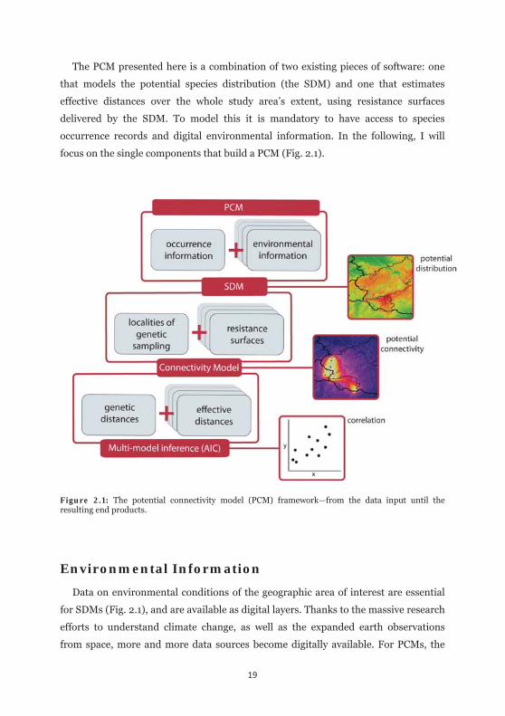
The PCM presented here is a combination of two existing pieces of software: one
that models the potential species distribution (the SDM) and one that estimates
effective distances over the whole study area’s extent, using resistance surfaces
delivered by the SDM. To model this it is mandatory to have access to species
occurrence records and digital environmental information. In the following, I will
focus on the single components that build a PCM (Fig. 2.1).
Figure 2.1: The potential connectivity model (PCM) framework—from the data input until the resulting end products.
Environmental Information
Data on environmental conditions of the geographic area of interest are essential
for SDMs (Fig. 2.1), and are available as digital layers. Thanks to the massive research
efforts to understand climate change, as well as the expanded earth observations
from space, more and more data sources become digitally available. For PCMs, the
20
spatial resolution of these data sources depends on the study question, the spatial
scale of interest, the study extent and, of course, the data availability. Most SDM
applications that focus on the macro-scale to work on biogeographic research
questions use interpolated climate information that are globally available in different
spatial resolutions ranging from 10 arc minutes down to 30 arc seconds (HIJMANS et
al. 2005). These climate data are available as monthly averages over the past 50
years, which can be used to calculate biologically relevant (i.e., bioclimatic) variables.
They also cover possible future (following IPCC climate change scenarios) and past
scenarios, covering for instance the mid-Holocene climate optimum, the last glacial
maximum and the last interglacial period.
Next to climatic information, there are datasets available that globally cover
topography and land use. Topographic information is available in resolutions as fine
as 30 meters (SRTM Shuttle Mission), while processed data on land cover classes are
available at 300 meter resolution (PFEIFER et al. 2012). Some studies show that the
use of landscape parameters derived from remote sensing can improve SDM
predictions, as opposed to using bioclimatic information alone (CORD & RÖDDER
2011).
In the past few years, more and more fine-scale remote sensing data become
available for large parts of the world. This would even allow for the spatially explicit
modeling of habitat suitability for locally restricted areas. The resolution here is at 30
meters or below and can be as fine as one meter for some data products. This allows
for the analysis of entirely new study questions, such as the characterization of
potential distribution or habitat suitability, or the assessment of demographic
processes like abundance (VANDERWAL 2009) or reproductive success (BRAMBILLA &
FICETOLA 2012)—all especially useful in the environmental management sector. My
own preliminary study revealed that the prediction of butterfly abundance is
impossible to make by using coarse-scaled climatic information alone (FILZ et al.
2013b); fine-scale environmental information is therefore mandatory to allow for the
inference and prediction of such processes.
Depending on the question of interest, I use very different spatial layers for PCMs
in my thesis. While applications for environmental planning need fine-scaled
environmental information, it is more practical to use coarse-scaled environmental
predictors in landscape genetic studies that cover large extents.
21
Occurrence Informaton
For the computation of an SDM, occurrence records from the focal species are
needed (Fig. 2.1). The spatial scale (or, resolution) of these occurrence records
(defined as grain; FRANKLIN 2009), would need to at least be as fine as the respective
environmental layer. If, for instance, occurrences recorded at a large grain (e.g.,
records resulting from a 100 m wide transect) were modeled against environmental
layers of a finer resolution (e.g. grids of 25 m), then they could be falsely linked to a
neighboring grid cell with different environmental conditions (MEYER & THUILLER
2006; GUISAN et al. 2007). Consequently, these inaccurate occurrences could yield an
erroneous model output, as the forecasted habitat suitability would get blurred by
wrongly assigned environmental conditions that are actually unsuitable for the
species. This effect, however, decreases with decreasing resolution of the
environmental layers and is less important for coarse-scaled environmental layers
(THOMAS et al. 2002; GUISAN et al. 2007).
The SDM
Species distribution models, habitat suitability models or environmental niche
models all follow the same principle: they link spatially explicit information about the
presence (or, absence) of a species to the environmental conditions in geographic
space with a predictive model (FRANKLIN 2009). The value ranges of these
environmental predictors (or, variables) at the presence locations are compared with
the environmental conditions found at absence locations or a defined set of random
locations (i.e., the background or pseudo-absences). Depending on the algorithm, the
model will be calculated and projected to a defined geographic area, together with an
estimate of variable importance.
In the last couple of years, this framework has become widely applied in different
fields of ecology and evolution (FRANKLIN 2009; PETERSON et al. 2011), such as in
conservation biology (e.g., ARAÚJO et al. 2004; GUISAN & THUILLER 2005; KREMEN et
al. 2006; RÖDDER et al. 2010), invasion biology (e.g., PETERSON & VIEGLAIS 2001;
FICETOLA et al. 2007; STIELS et al. 2011) climate change biology (e.g., IHLOW et al.
2012), evolutionary biology (e.g., KOZAK et al. 2008; KOZAK & WIENS 2007, SMITH &
DONOGHUE 2010; ENGLER et al. 2013), biodiversity research (e.g., CARNAVAL & MORITZ
22
2008; SCHIDELKO et al. 2011) and as an additional tool in phylogenetic reconstruction
(e.g., KOZAK & WIENS 2007; CHAN ET AL. 2011; RÖDDER et al. 2013). The number of
algorithms is as diverse as their fields of application. In this thesis, I focus on the
software MAXENT (PHILLIPS et al. 2004; PHILLIPS et al. 2006; PHILLIPS & DUDÍK 2008).
MAXENT is a machine-learning algorithm derived from the field of artificial
intelligence and follows the principle of maximum entropy (JAYNES 1957; ELITH et al.
2011). Among the many competing methods, MAXENT always ranked among the top
performing approaches (e.g., ELITH et al. 2006; HEIKKINNEN 2006; HERNANDEZ et al.
2006; POULOS et al. 2012)—even under limited species occurrence information (e.g.
WISZ et al. 2008)—and is known to be tolerant against multicollinearity, as long as
model results are not projected (e.g., PHILLIPS et al. 2006; BRAUNISCH et al. 2013).
Detailed model specifications follow in the respective chapters. MAXENT’s resulting
map highlights the occurrence probability of the study area, which can be used to
identify regions that are potentially suitable or unsuitable. These probability values
are logistically distributed and cover a range between 0 (no predicted occurrence)
and 1 (highest probability for occurrence).
Thresholds applied to this distribution of values can cut off low values that can be
seen as noise and do not contribute to potential distribution. These thresholds should
be dynamic and not fixed (LIU et al. 2005). This is because the data settings are
different for each model and depend on the number and position of occurrence
records, the extent and position of the study area, and the number of environmental
predictors used for modeling. Since thresholds follow fixed deterministic rules, they
remain comparable in their validity. A conservative threshold, for instance, would be
based on the lowest estimated occurrence probability measured at a given set of
occurrences used for model training (i.e., minimum training presence). In contrast, a
more sensitive threshold would set this limit higher by omitting the lowest 10% of the
occurrence probability measured at the respective set of presence records (i.e., 10th
percentile training presence).
For the PCM, these thresholds can optionally be used as fragmentation thresholds
(ANDRÉN 1994; METZGER & DÉCAMPS 1997) that highlight absolute barriers to
structural connectivity. From this, the modeled map of potential suitability will turn
into a resistance surface of the study area, which can be fragmented when such
thresholds are applied.
23
The Connectivity Model
The prepared resistance surface can now be used in a connectivity model to
estimate effective distances among sample sites (Fig. 2.1). Here, I use the software
CIRCUITSCAPE, which is based on electric circuit theory and follows the principles of
Ohm’s law (MCRAE & BEIER, 2007; MCRAE et al. 2008). CIRCUITSCAPE allows the
assessment of multiple connections in the study area, and thus is not restricted to the
limits of the least cost path framework and as consequence outcompetes LCP models
(MCRAE & BEIER 2007). The estimated effective distances can be used either for
comparisons with genetic distances (see below) estimated from individuals sampled
at the same locations, or for visualizing the potential connectivity among the
considered locations across the study area for management purposes.
Linking genetic information with PCMs
Information about the genetic differentiation (i.e. the genetic distance) of a focal
species in a study area can be correlated to the estimated effective distances
measured by the PCM (Fig. 2.1). Genetic distances can be measured with different
metrics, such as FST (WRIGHT 1965) or Dest (JOST 2009). To understand the relative
importance of certain landscape elements, multiple resistance surfaces can be
modeled and subsequently compared to genetic distances. For the correlation of
genetic distances with effective distances, many different methods exist (BALKENHOL
et al. 2009). Here, I used a multi-model inference approach, based on linear
regressions, which compares effective distances from competing resistance surfaces
and finds the set of landscape elements with the highest information content. Model
importance is not tested here by using classic null hypothesis significance testing, but
instead through maximum likelihood methods based on information theory, the
Akaike information criterion (AIC; BURNHAM & ANDERSON 2002; JOHNSON & OMLAND
2004). AIC evaluates different models given their explained information content and
ranks them according to their importance. Differences between AIC values among the
models inform about their importance. A general rule is that a model is considered
best if the difference between the AIC in the highest ranked model and the next
largest AIC value (delta or ) is >2. If there are one or more models of < 2, then
they need to be considered together with the highest ranked model (BURNHAM &

24
ANDERSON 2002). The main advantage of this method is that the non-independent
data structure of pairwise comparisons—a classical error in statistics—is the same for
each model. Hence, the non-independence error cannot influence the relative ranking
of the candidate set of models used in the comparison.
Taken together different tools and information into a single framework as outlined
above, offers new opportunities to quantify connectivity for environmental planning,
to find limiting environmental conditions for genetic exchange, and to widen our
understanding of species distribution as a whole. In the following chapters I will
discuss the need for such a holistic perspective and exemplify how PCMs can
contribute to different aspects, when fed with real data.

25

26

27
PART APCM’S IN CONSERVATION &
ENVIRONMENTAL PLANNING

28

29
CHAPTER 3
Accounting for the ‘network’ in the Natura 2000 network: A
response to Hochkirch et al. 2013
“The more “connected” we become, non-human life with which we share this planet becomes increasingly disconnected.”
KEVIN R. CROOKS & M SANJAYAN

30
This chapter has been published on the ArXiv preprint server: arXiv:1408.7076
The work was conducted in collaboration with ANNA F. CORD from the Helmholtz Centre for Environmental Research, PETRA DIECKER from the Institute of Ecology at the Leuphana University Lüneburg, as well as WOLFGANG J. WÄGELE and DENNIS RÖDDER from the Zoological Researchmuseum Koenig.
31
Commentary
Worldwide, we are experiencing an unprecedented, accelerated loss of biodiversity
triggered by a bundle of anthropogenic threats such as habitat destruction,
environmental pollution and climate change (BUTCHART et al. 2010). Despite all
efforts of the European biodiversity conservation policy – initiated 20 years ago by
the Habitats Directive (EU 1992) that provided the legal basis for establishing the
Natura 2000 network – the goal to halt the decline of biodiversity in Europe by 2010
has been missed (EEA 2010). HOCHKIRCH et al. (2013) identified four major
shortcomings of the current implementation of the directive concerning prioritization
of the annexes, conservation plans, survey systems and financial resources. They
hence proposed respective adaption strategies for a new Natura 2020 network to
reach the Aichi Biodiversity Targets.
Despite the significance of these four aspects, HOCHKIRCH et al. (2013) did not
account for the intended ‘network’ character of the Natura 2000 sites, an aspect of
highest relevance. Per definition, a network requires connective elements (i.e.
corridors) between its nodes. From an ecological perspective, the Natura 2000
network must guarantee that the species of concern are able to exchange between
habitat patches (above all for maintaining/fostering gene flow; e.g., STORFER et al.
2007). Several studies have shown that reserves fail to protect the species they were
designed for due to their isolated character in an anthropogenically degraded
landscape matrix (e.g., SEIFERLING et al. 2012), even though they are well managed
(FILZ et al. 2013a). In turn, habitat connectivity greatly enhances the movement of
species within fragmented landscapes (GILBERT-NORTON et al. 2010). Both Habitats
(Art. 10) and Birds Directive (Art. 3) explicitly mention the importance of elements
providing functional connectivity (‘ecological coherence’) outside the designated
Special Areas of Conservation (SACs) for species of Community interest. However,
since the member states are responsible for the designation of SACs, their selection
often represents a consensus of various political, economic and ecological
considerations. This weakness is well acknowledged in a guidance document from the
Institute for European Environmental Policy (KETTUNEN et al. 2007). The authors
formulated a framework for assessing, planning and implementing ecological
connectivity measures in a way that is legally binding and standardized across
borders. Additionally, they presented measures increasing habitat connectivity and

32
future research needed on this topic. Besides the strategies proposed by HOCHKIRCH
et al. (2013), there is hence an urgent need to investigate the inter-reserve
connectivity in the Natura 2000 network as a whole and specifically for the priority
species for which SACs have been designated. Recent software developments and the
increasing availability of high-resolution environmental data in combination with
extensive fieldwork will help to meet these research requirements. Finally, the results
derived from such research must be implemented into a binding EU-legislation as
well as a standardized planning policy across national borders to reach scientific
consensus on corridor design, which often lacked in the past (BENNETT et al. 2006).
This might ultimately ensure an ecological coherence between SACs, which is the
prerequisite, over any other strategies, ensuring a Natura 2020 network being worth
its name.

33

34

35
CHAPTER 4
Missing the target? A critical view on butterfly conservation
efforts on calcareous grasslands in south-western Germany
“Like the resource it seeks to protect, wildlife conservation must be dynamic, changing as conditions change, seeking always to become more effective.”
RACHEL CARSON

36
This chapter has been published in Biodiversity & Conservation 22: 2223-2241 (2013).
The work was conducted in collaboration KATHARINA J. FILZ and THOMAS SCHMITT from the Biogeography Department of the University of Trier, JOHANNES STOFFELS from the Department of Remote Sensing at the University of Trier, as well as Matthias Weitzel from Trier.
37
Introduction
Europe is undergoing a continuous period of invertebrate decline (VAN SWAAY et al.
2011). In particular, the loss of typical habitats like semi-natural grasslands due to
intensive agriculture and urban development has been particularly dramatic for
butterfly species (BOURN & THOMAS 2002; VAN SWAAY 2002; WENZEL et al. 2006). In
this aspect, calcareous grasslands of south-western Europe are considered to be one
of the most important habitat types for insect conservation (VAN SWAAY 2002;
WALLISDEVRIES et al. 2002). These habitats contain a renowned biological diversity
including a variety of species listed under the habitat directive of the Bern Convention
(VAN HELSDINGEN et al. 1996). 274 (i.e., 48%) of the 576 butterfly species reported as
native in Europe occur on calcareous grasslands. Moreover, from the 71 species
considered threatened in the same area, 37 (i.e., 52%) can be found in theses habitats
(VAN SWAAY 2002). Consequently, many calcareous grasslands are protected as
nature reserves and are integrated in the Natura 2000 program of the European
Union (VAN SWAAY et al. 2011). However, even such legally protected sites continue to
be lost or are still losing species despite protection. As a result, many specialized and
rare species are now threatened or already extinct (WARREN 1997; WENZEL et al.
2006).
Many European countries are experiencing similar population declines. The
Netherlands have lost over 24% of its butterfly fauna (WYNHOFF & VAN SWAAY 1995)
and 30% of the indigenous species became extinct in Flanders during the 20th
century (MAES & VAN DYCK 2001). In Britain, nearly nine percent of the resident
butterfly species have gone extinct (WARREN 1997) and in Moravia (Czech Republic)
BENES & KURAS (1998) recorded a 60% loss of butterflies during the same time
period. The decline of butterflies has caused an increasing concern in Western
Europe and the subsequent implementation of conservation activities for Lepidoptera
and other wildlife (THOMAS 1995; VAN SWAAY & WARREN 2006; VAN SWAAY et al.
2011).
The prevalent conservation strategy has been to designate threatened habitat types
as nature reserves. The habitat types most deserving protection have been identified
by the conservation value of the habitat itself and/or by the presence of a great
number of rare and endangered species. Until today, such biodiversity assessments
have been the major tool in conservation planning and implementation. However,
38
this strategy has had the negative effect of frequently creating small habitat patches
isolated by unsuitable, unprotected landscape, which prevents the inter-patch
exchange of species. Moreover, small habitat patches may lack the possibility to
buffer large-and meso-scale environmental effects (for a discussion see HOF et al.
2011). Habitats are lost due to diverse land-use changes, which do not necessarily
stop at the margin of protected areas, but also changes subtly the characteristics of
semi-natural grasslands (DOVER & SETTELE 2009). The negative impacts of nutrient
and pesticide loads as well as climatic changes influence the habitat structure as well
as microclimatic conditions (PARMESAN 2006; BARTHOLMESS et al. 2011). Frequently,
a loss of plant diversity and changes in plant communities is followed by butterfly
declines, and especially species with high specialization on particular food plants
might be affected (e.g., WARREN et al. 2001; POLUS et al. 2007).
Besides the impacts of agricultural improvements on adjacent patches,
abandonment is considered to be one major threat to semi-natural habitats (VAN
SWAAY 2002). As many butterfly species depend on the preservation of habitats
created by extensive human land-use activities, habitat management is considered to
play a crucial role for the practical conservation of threatened species (WARREN
1993a,b). Many species are restricted in their local distribution to these often small
and fragmented remnants making them susceptible for any change in habitat quality
(DOVER & SETTELE 2009). As a consequence, today species conservation is more than
ever a question of protecting habitats in a changing environment, but also to retain
species diversity within small and fragmented habitats.
However, the lack of habitat quality and habitat connectivity have led to decreasing
numbers of butterfly species not only in legally protected semi-natural habitats, but
even more severely in unprotected agricultural areas (DOVER & SETTELE 2009). In the
latter, remnants of pre-industrial human land-use (e.g. as fallow grounds) are today
considered to belong to the most species rich habitats in these areas (SCHMITT &
RÁKOSY 2007). These fallows act as retreats as well as stepping stones for many
specialized taxa, consequently turning into habitats with high conservation value
(WEIBULL 2000; SCHMITT & RÁKOSY 2007; SCHMITT et al. 2008; LIZÉE et al. 2011).
Agricultural areas adjacent to fallow grounds affect population dynamics and
community structures within these habitats. Additionally, the ongoing loss of
stepping stones reduces overall habitat area and landscape connectivity. Hence, patch
size and isolation, as well as missing management activities often favor the
39
vulnerability of this habitat type to environmental effects. Consequently, the decline
of butterfly species should proceed even faster in cultivated landscapes than in
protected areas.
In this study, we aim to identify the mechanisms responsible for the vulnerability
of butterfly species and their habitats using the examples of calcareous grasslands
and fallow grounds. We intensively re-investigated butterfly communities after a 40-
year time period within a defined region of south-western Germany in both managed
and legally protected as well as unmanaged grasslands. Regarding the location,
geographical integration and management activities of the different grasslands, we
evaluate the connectivity of specific habitat types in the landscape and discuss the
possible impacts of recent land-use changes and local global warming on the stability
of functional trait diversity in butterfly communities. In particular, we assess whether
and how butterfly species richness and community composition in managed versus
unmanaged grasslands have changed over the last decades and discuss the
appropriateness of conservation strategies for nature reserves.
Material and methods
Study sites
Our study area is located at the south-western boarder of Germany (Fig. 4.1a). The
vicinity of Trier is characterized by a long tradition of human settlement.
Anthropogenic land-use created a manifold mosaic of habitat types ranging from
vineyards, agricultural fields, fallows, flower rich meadows, woodlands, rivers and
floodplains to several semi-natural habitats like calcareous grasslands. Today,
traditional farming systems and semi-natural habitats, which ensured the survival of
a diversity of species for thousands of years, are replaced by intensive cultivated
agricultural areas. Since the middle of the 20th century, land-use changes have
caused serious consequences for the conservation of these traditional habitats as their
quality and quantity have declined. Habitats are being lost due to, intensive
agricultural usage, anthropogenic loads of nutrients and the failure of extensive
management, which lead to advanced succession and final loss of these habitats
(BURGGRAAFF & KLEEFELD 1998).
40
Calcareous grasslands
For our study, we selected six calcareous grasslands. During the last 40 years, the
patches remained as grassland and five of them are preserved as nature reserves.
Calcareous grasslands rank among the most species-rich habitats in Europe (VAN
SWAAY 2002) and are classified as highly endangered in the Red List of endangered
habitat types in Rhineland-Palatinate. A strong decline of these habitats has already
been observed during the last decades in our study area (BIELEFELD 1985; WENZEL et
al. 2006; M. WEITZEL own observations.) and even legally protected sites continue to
decline (WENZEL et al. 2006).
The phytocoenosis of the study sites can be described as Mesobromion errecti
dominated by flowering herbs and grasses (e.g., Bromus errectus, many
Orchidaceae), interspersed with single stands of shrubs (e.g., Crataegus monogyna,
Prunus spinosa) or small trees. Vegetation varied in height throughout the year, but
in general was corresponding to the dominating plant species less than 30 cm high.
In four reserves, structural characteristics were preserved by tending strategies
(mowing and clearing). Like most semi-natural habitats, the patches were highly
fragmented and under external pressure from agricultural intensification and
changing land-use. The degree of isolation, calculated using the formula of POWER
(1972), varied between 78.8% (Echternacherbrück) and 99.9% (Kelsen). The isolation
of the investigated habitats can be explained by natural limiting factors like the
geological condition, microclimatic factors or by anthropogenic fragmentation.
In total the study sites extended over 136 ha, which represent a considerable
proportion of the 752 ha of calcareous grasslands known in Rhineland-Palatinate
(KLEIN et al. 2001). The minimum geographic distance between patches was 3 km
between Igel and Wasserliesch. In the other cases, distances exceeded 10 km. Spatial
autocorrelation among sites could be excluded.
Patch size varies considerably from 1.5 ha (Kelsen) to 68 ha (Echternacherbrück).
Depending on the total size of the reserve, one to four transects per patch (transect
length 40-385 m) were established in 1972. All transects were re-established and re-
investigated in 2011 in cooperation with the initial observer (M. WEITZEL).
Vineyard Fallows
41
Eight xerothermic vineyard fallows were selected for field surveys. Theses patches
were structurally young fallows in 1973 and have been abandoned from agricultural
use for at least fifty years. Old fallows are considered to hold a significantly higher
species richness and heterogeneity and host more Red List species than earlier stages
(BALMER & ERHARDT 2000). Vegetation height varied throughout the year, but on
average did not exceed 80 cm. The vegetation was dominated by perennial bunch
grasses, a variety of thermophilic flowering herbs as Onobrychis vicifolia, Daucus
carota, Centaurea ssp., Medicago ssp., Vicia spp, Rumex ssp. and few interspersed
hedge structures composed of Rosa ssp., Rubus ssp., Cytisus scoparius and
Crataegus monogyna. Geological conditions and microclimatic factors prevent the
vegetation of converting into secondary forests. Moreover, structural characteristics
have been maintained by occasional extensive sheep pasturing. All patches suffer
from a high degree of fragmentation as well as external pressure from adjacent
intensively cultivated farmland (mostly vineyards), hay meadows and housing areas.
Minimum distance between patches was 200 m (Brettenbach I; Brettenbach II). In
the other cases, geographic distances were on average 1.6 km. A spatial
autocorrelation among patches could be excluded. Patch size varied between 2.7 ha
(Kernscheid) and 5.8 ha (Brettenbach I). In total, the studied vineyard fallows
extended over 34.5 ha. In 1973, one transect of varying length (432-1430 m) was
established per patch. The transects were re-established and re-investigated in 2010
in cooperation with the initial observer (M. WEITZEL).
Field sampling design
In both grassland types, data were taken from standardized transect counts along
fixed transects. The structure of this monitoring was similar to that described by
POLLARD & YATES (1993). Each butterfly seen within an observation radius of 5 m
ahead and 2.5 m on each side of the observer was counted. Individuals were either
identified and counted by sight or captured with a butterfly net for closer
determination to species level. If possible, each transect was visited every ten days
from April to October for a time period appropriate to their length. The observations
were conducted randomly between 10:00 am and 5:00 pm if weather conditions
permitted (POLLARD & YATES 1993; SETTELE et al. 1999), i.e., temperature above 17°C,
wind less than six Beaufort and no rain (VAN SWAAY et al. 2008). Variations due to
42
weather and time of day were counterbalanced by randomizing the visits. Records
were kept along with descriptions of weather conditions and recent management
activities. In total, 105 transect walks were performed in 2011 and a similar amount in
1972 on calcareous grasslands. 136 transect walks were conducted in 1973 and 109 in
2010 on vineyard fallows. To obtain unbiased data, observations were conducted
throughout the same time period each year using identical transects as well as field
methods.
Classification of butterfly species
We categorized all butterfly species regarding their national conservation status
and classified them into functional groups defined by habitat requirements, dispersal
behaviour, larval food plant specialisation and global distribution.
We used the classification of BINK (1992) for the analysis of dispersal abilities. For
increasing the statistical power, the nine dispersal classes were condensed to three:
sedentary species (class 1-3), mobile species (class 4-6) and migrants (class 7-9). We
used the classification of REINHARDT & THUST (1988) for general habitat requirements
to distinguish between ubiquitous, mesophilic, hygrophilic and xerothermophilic
species. Caterpillars were classified, respective to their food plant use, as
monophagous, oligophagous and polyphagous (EBERT & RENNWALD 1991). Global
distribution data were obtained from KUDRNA (2002). We classified butterfly species
as Mediterranean if their distribution area includes southern Iberia, southern Italy or
Greece, i.e. ensuring their survival in Mediterranean glacial refugia during the LGM.
The distribution areas of continental species usually exclude these regions and do not
reach the lowland areas along the coast of the Atlantic or the British Isles. These
species usually survived in the last glacial period in extra-Mediterranean and/ or
more eastern refugia. Species were classified as a Mediterranean-continental species
if their distribution area includes at least one of the areas typical for the
Mediterranean species, but also extends to the continental parts of Eurasia. The
classification of each species is given in Table 4.1.

43
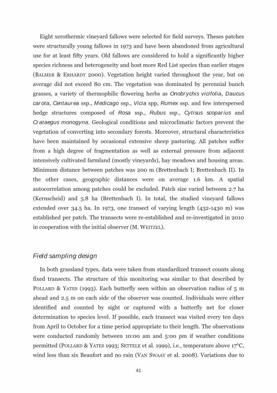
Table 4.1: Presence-absence data of all butterfly species recorded on six calcareous grasslands and on eight vineyard fallows with the number of study sites with the species being present in 1972/73 and 2010/11 including their species specific functional traits (D1: sedentary, D2: medium, D3: migrant; P1: monophagous, P2: oligophagous, P3: polyphagous; H1: xerothermophilic, H2: mesophilic, H3: hygrophilic, H4: ubiquitous; A1: Mediterranean, A2: continental, A3: continental-Mediterranean, A4: migrant)
Calcareous grasslands Vineyard fallows
1972 2011 1973 2010 Traits
Hesperidae Erynnis tages (L., 1758) 6 4 7 0 D1 P2 H1 A1 Carcharodus alceae (Esp., 1780) 1 0 7 0 D2 P2 H1 A1 Spialia sertorius (Hoff., 1804) 6 3 6 0 D1 P1 H1 A1 Pyrgus malvae (L., 1758) 6 5 8 5 D1 P2 H2 A1 Pyrgus serratulae (Ram., 1839) 1 0 0 0 D1 P1 H1 A3 Carterocephalus palaemon (Pal., 1771)
4 0 3 0 D1 P2 H2 A2
Thymelicus lineola (O., 1808) 6 6 8 6 D2 P2 H2 A2 Thymelicus sylvestris (Poda, 1761)
6 6 5 6 D1 P2 H2 A1
Thymelicus acteon (Rott., 1775) 3 0 0 0 D1 P2 H1 A1 Hesperia comma (L., 1758) 1 1 0 0 D1 P2 H2 A3 Ochlodes sylvanus (Esp., 1778) 6 3 8 4 D2 P3 H4 A1 Papilionidae Papilio machaon (L., 1758) 6 5 8 6 D2 P3 H2 A1 Pieridae Leptidea sinapis (L., 1758)/ reali (Reiss, 1989)
6 6 8 8 D2 P2 H2 A1
Anthocharis cardamines (L., 1758)
6 5 8 8 D2 P2 H2 A3
Aporia crataegi (L., 1758) 5 3 6 5 D2 P2 H2 A1 Pieris brassicae (L., 1758) 6 6 8 3 D3 P3 H4 A1 Pieris rapae (L., 1758) 6 6 8 8 D2 P3 H4 A1 Pieris napi (L., 1758) 6 6 8 6 D2 P3 H4 A1 Pontia daplidice (L., 1758) 1 0 0 0 D2 P3 H1 A1 Colias croceus (Fourc, 1785) 3 0 2 0 D3 P2 H4 A4 Colias hyale (L., 1758) 6 4 8 6 D2 P2 H2 A2 Colias alfacariensis (Rib., 1905) 5 1 0 0 D2 P2 H1 A1 Gonepteryx rhamni (L., 1758) 6 6 8 7 D2 P2 H2 A1 Lycaenidae Hamearis lucina (L., 1758) 5 0 5 0 D1 P1 H2 A2 Lycaena phlaeas (L., 1761) 6 4 8 6 D2 P1 H2 A1 Lycaena dispar (Haw., 1803) 0 0 0 1 D2 P1 H3 A2 Lycaena tityrus (Poda, 1761) 6 2 8 3 D1 P1 H2 A3 Lycaena hippothoe (L., 1761) 0 0 1 0 D1 P1 H3 A2 Thecla betulae (L., 1758) 6 2 8 1 D1 P1 H2 A2 Neozephyrus quercus (L., 1758) 4 0 3 0 D1 P1 H1 A3 Satyrium ilicis (Esp., 1779) 4 0 0 0 D1 P1 H1 A3 Callophrys rubi (L., 1758) 6 6 8 5 D2 P3 H2 A1 Satyrium w-album (Knoch, 1782) 0 0 3 0 D1 P1 H2 A2 Satyrium pruni (L., 1758) 6 3 8 0 D1 P1 H1 A2 Satyrium acaciae (Fab., 1787) 3 0 0 0 D1 P1 H1 A3 Cupido minimus (Fues., 1775) 6 6 4 0 D1 P1 H1 A3 Cupido argiades (Pallas, 1771) 0 0 0 2 D2 P2 H1 A2 Celastrina argiolus (L., 1758) 6 3 8 1 D2 P3 H2 A3 Maculinea arion (L., 1758) 3 0 0 0 D1 P2 H1 A3 Aricia agestis (Den.&Schiff., 1775)
6 6 0 7 D2 P3 H1 A1
Polyommatus semiargus (Rott., 1775)
6 6 7 7 D2 P1 H2 A1
Polyommatus icarus (Rott., 1775) 6 6 8 7 D2 P2 H4 A1 Polyommatus coridon (Poda, 1761)
6 5 4 0 D2 P1 H1 A1
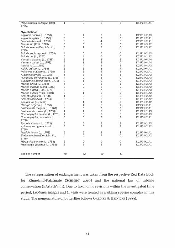
44
Polyommatus bellargus (Rott., 1775)
1 0 0 0 D1 P2 H1 A1
Nymphalidae Argynnis paphia (L., 1758) 6 4 8 1 D2 P1 H2 A3 Argynnis aglaja (L., 1758) 6 5 7 3 D1 P1 H2 A1 Issoria lathonia (L., 1758) 6 5 4 6 D2 P1 H2 A1 Brentis ino (Rott., 1775) 0 0 2 0 D1 P2 H3 A2 Boloria selene (Den.&Schiff., 1775)
6 1 8 0 D1 P1 H3 A2
Boloria euphrosyne (L., 1758) 4 0 0 0 D1 P1 H2 A3 Boloria dia (L., 1767) 0 4 0 0 D2 P1 H1 A2 Vanessa atalanta (L., 1758) 6 3 8 5 D3 P1 H4 A4 Vanessa cardui (L., 1758) 6 1 8 0 D3 P3 H4 A4 Inachis io (L., 1758) 6 4 8 8 D2 P3 H4 A3 Aglais urticae (L., 1758) 6 6 8 7 D2 P1 H4 A1 Polygonia c-album (L., 1758) 6 3 8 4 D2 P3 H2 A1 Araschnia levana (L., 1758) 6 3 8 5 D2 P1 H2 A2 Nymphalis polychloros (L., 1758) 4 0 3 0 D2 P3 H2 A3 Euphydryas aurinia (Rott., 1775) 0 1 0 0 D1 P2 H3 A3 Melitea cinxia (L., 1758) 6 0 3 1 D1 P1 H2 A3 Melitea diamina (Lang, 1789) 2 0 6 0 D1 P1 H3 A2 Melitea athalia (Rott., 1775) 6 3 7 2 D1 P3 H2 A3 Melitea aurelia (Nick., 1850) 2 1 0 0 D1 P3 H1 A2 Limentis populi (L., 1758) 1 0 2 0 D1 P1 H2 A2 Limentis camilla (L., 1764) 5 0 6 0 D1 P1 H2 A2 Apatura iris (L., 1764) 5 1 1 0 D1 P1 H2 A2 Pararge aegeria (L., 1758) 6 4 8 1 D2 P2 H2 A1 Lasiommata megera (L., 1767) 6 5 7 3 D2 P2 H2 A1 Lasiommata maera (L., 1758) 1 1 0 0 D1 P2 H1 A3 Coenonympha arcania (L., 1761) 4 6 8 5 D1 P3 H2 A3 Coenonympha pamphilus (L., 1758)
6 6 8 7 D1 P3 H2 A1
Pyronia tithonus (L., 1771) 6 6 8 8 D1 P2 H1 A3 Aphantopus hyperantus (L., 1758)
6 6 8 7 D1 P3 H2 A2
Maniola jurtina (L., 1758) 6 6 8 8 D2 P3 H4 A1 Erebia medusa (Den.&Schiff., 1775)
4 0 7 0 D1 P3 H2 A2
Hipparchia semele (L., 1758) 2 0 0 0 D2 P3 H1 A1 Melanargia galathea (L., 1758) 6 6 8 8 D1 P2 H2 A1 Species number 70 52 59 41
The categorisation of endangerment was taken from the respective Red Data Book
for Rhineland-Palatinate (SCHMIDT 2010) and the national law of wildlife
conservation (BArtSchV §1). Due to taxonomic revisions within the investigated time
period, Leptidea sinapis and L. reali were treated as a sibling species complex in this
study. The nomenclature of butterflies follows GAEDIKE & HEINICKE (1999).
45
Statistical analysis
For each study patch, we constructed a data matrix containing the presence-
absence data of all recorded butterflies. Species estimate accuracy was calculated
computing expected species accumulation curves (sample-based rarefaction curves)
and incidence-based richness estimators (Chao1, Chao2, ICE, first-order jackknife,
Michaelis-Menten) using ESTIMATES WIN 8.00.
Differences in species composition between the study years were evaluated for
each study patch. Tests among study sites and observation years were done by
Wilcoxon tests, Cochran Q tests and 2 tests for heterogeneity in SPSS 15.0. We also
performed separate statistical calculations for each functional group using Cochran-
Q-tests to analyse community shifts between the observation years.
Turn-over rates were estimated for both grassland types to identify the changes of
the faunas between the two observation years in MICROSOFT EXCEL 2003. It was
calculated as the number of species recorded in only one of the observation years
divided by the total number of species observed during both observation years.
Comparisons of the similarity of the community structures were made using the
Sørensen similarity index. It was calculated on the basis of presence/absence data as
the number of shared species divided by the number of species in the two samples,
respectively.
Independently from changes in absolute species composition, we evaluated
changes in relative functional trait diversity by using PCA in combination with linear
discriminant analysis (LDA) in SPSS. We calculated relative proportions for the
functional trait classes separately for each site and time slice. In consequence, each
trait (Dispersal: 3 classes; Foodplant use: 3 classes; Habitat: 4 classes, Distribution 4
classes) was summed to 1 on each side. This information was thereafter transformed
via PCA into a multivariate scenopoetic trait space by taking principal components
that exceeds the value of one after conducting a varimax rotation. Group
discrimination (i.e. taking year as grouping variable) was tested thereafter using
cross-validated LDA.
To test for differences in parallelism of the community shifts between calcareous
grasslands and the vineyard fallows, we performed a circular ANOVA using the
circular package in R (JAMMALAMADAKA & SENGUPTA 2001; R DEVELOPMENT CORE
46
TEAM 2010), where the directions of each vector connecting the two observation years
in the PCA-space were used as dependent factor.
Resistance surface modeling
To infer patterns of habitat fragmentation in both habitat types, we combine an
environmental niche model with a habitat connectivity model using fine-scale
environmental GIS-layers as predictors for model building. The environmental layers
comprise four different vegetation indices based on multispectral ASTER (Advanced
Space Borne Thermal Emission and Reflection Radiometer) data in 30 m resolution
(NDVI, NDWI, soil-brightness, vegetation-greenness) as well as topography
information derived from the ASTER global digital elevation map of the same
resolution (altitude, slope, aspect). Further, we used categorical CORINE landcover
data of 2006 (available through: eea.europe.com) with a resolution of 100 m. The
Normalized Different Vegetation Index (NDVI), developed by ROUSE et al. (1974), is a
simple vegetation index for remotely sensed data that quantifies the density of plant
growth on earth, and so provides information about vegetation biomass (JENSEN
2007). The calculation of the Normalized Difference Water Index (NDWI),
introduced by GAO (1996), provides information about the vegetation water content
and allows assessments to be made of changes in plant biomass and water stress of
vegetation.
Suitable satellite data for the purpose of a study like this need to have a sufficient
spectral resolution to ensure a spectral discrimination of different land cover types.
Furthermore, a high spatial resolution is required to accurately depict small
landscape structures. The ASTER multispectral imager onboard NASA’s Terra
satellite is largely compliant with these requirements. ASTER has three separate
imaging subsystems which cover the visible and near infrared (VNIR), the shortwave
infrared (SWIR) and the thermal infrared (TIR) spectral ranges with 3, 6 and 5
spectral bands with spatial resolutions of 15 m, 30 m and 90 m (YAMAGUCHI et al.
1999; ABRAMS 2000). In this study, one ASTER scene (acquisition date: June 26,
2001), covering the northern and central parts of Rhineland-Palatinate was selected
for analysis.
47
ASTER spectral bands 1-4, primarily designed for assessing vegetation properties,
were selected. From the especially narrow band in the 2-2.5 μm range, conceptualized
mainly for the purpose of surface soil and mineral mapping (YAMAGUSHI et al. 1998),
a single broad bandwidth channel centered at 2.2 μm was synthesized by averaging
channel 5-7, thereby prioritizing improved signal-to-noise ratio versus spectral
resolution considered less important for the study purpose. No Thermal bands were
used in this study.
Since remote sensing data with medium spatial resolution has only been of limited
use for the identification of species compositions (WULDER 1998), the reduced spatial
resolution of the ASTER channels in the SWIR Range (i.e. 4 and the synthesized
channel 5) has been adjusted to match the 15-m pixel size of the visible and near-
infrared bands (1-3). The data fusion was performed with a local correlation approach
that preserves the spectral characteristics of the low resolution input and transfers
the textural properties of the high resolution reference to the ASTER-SWIR channels
(HILL et al. 1999).
The ASTER-scene was calibrated by converting the original digital numbers to
absolute reflectance values for each pixel based on ASTER calibration functions
(YAMAGUCHI et al. 1999; ARAI & TONOOKA 2005) and full radiative transfer modeling
(ATCPRO©; HILL & STURM 1991; HILL & MEHL 2003) based on the 5S Code by TANRÉ
et al. (1990). As the terrain of the study area is very mountainous, the removal of
topographic effects is important prior to the analysis of landscape structures. On
basis of the ATCPRO© model, terms describing illumination can be approximated by
the integration of a digital elevation model and finally compensated for each raster
cell of the dataset. In addition to the radiometric correction, the data preprocessing
comprised a precise georectification. The resulting ortho-projected datasets were
referenced to the national Gauss-Krüger coordinate system with sub-pixel accuracy
and later projected onto the classical WGS reference system using ARCGIS 9.3,
thereby fulfilling all requirements for an efficient integration of external geodata.
The Tasseled Cap Transformation (KAUTH & THOMAS 1976) could be described as a
guided and scaled linear transformation, which transforms the input satellite data
into three (or four) bands of known characteristics. A Tasseled Cap Transformation
was applied to the ASTER scene, and three thematic bands representing: soil-
brightness, vegetation-greenness and soil- and vegetation-wetness were derived.
48
Within the study extend (Fig. 4.1a), georeferenced locations of the respective habitat
type were set by visual inspection of aerophotos (using Google Earth) and during
several field surveys resulting in 12 and 34 locations for either habitat type,
respectively.
Environmental niche models were computed using MAXENT 3.3.3k, a machine
learning algorithm based on the principles of maximum entropy (PHILLIPS et al.
2006; PHILLIPS et al. 2008; ELITH et al. 2011). MAXENT has frequently outperformed
other approaches, especially when the number of georeferenced locations is scarce
(e.g. HERNANDEZ et al. 2006; ELITH et al. 2006; WISZ et al. 2008). Thus, this
algorithm became the method of choice. We used the standard settings, randomly
splitting the dataset into a 70% training and a 30% testing subset and using a
bootstrap approach between 100 different replicate runs to average model output.
Variable importance was assessed by jackknifing the training datasets. The output
was scaled in a logistic format. Despite recent criticisms (LOBO et al. 2008; JIMÉNEZ-
VALVERDE 2011), but in lack of other alternatives (e.g. BALDWIN 2009), AUC statistics
(SWETS 1988; FIELDING & BELL 1997) were used, as implemented in MAXENT, to
validate model performance. As threshold for identifying areas of low suitability
probability, we used the non-fixed equal training sensitivity and specificity threshold
as previously recommended (LIU et al. 2005). Connectivity between study sites in
either habitat was assessed depending on habitat specific suitability maps within a
connectivity model.
Here, we used the program CIRCUITSCAPE V. 3.4.1 (MCRAE & BEIER 2007; MCRAE et
al. 2008), which calculates pairwise resistance values between a defined set of
locations (here: habitat specific study sites). CIRCUITSCAPE is based on circuit theory
recently adapted from electrical engineering for the solution of landscape ecological
problems (MCRAE et al. 2008). By incorporating multiple pathways, CIRCUITSCAPE
reproduces connectivity between sites more accurate and with higher biological
relevance than more classical approaches like isolation-by-distance models or least
cost path models (MCRAE & BEIER 2007).
Prior to analysis, habitat suitability maps as derived from MAXENT models were
retransformed by multiplication of each probability by 10000 and again saved as
integer value, to reduce calculation time derived from long decimals, but without loss
of information (B. MCRAE pers. comm.). Further, values below the previously defined
49
absence threshold were set to the defined positive minimum integer value (i.e.,
setting to a value of 1) indicating highest resistance in those areas. Generally, the
habitat suitability map acts as conductance surface for the connectivity model. This
means that the higher the resistance, the lower the value is. Circuitscape was run in
four-node mode to safe computing time. For comparison of resistance values, we
used the site location used to build the resistance surfaces because they cover the
entire study extent. Depending on the difference of absolute location numbers, we get
561 pairwise comparisons for fallow grounds and 66 pairwise comparisons for
calcareous grasslands.
To obviate misleading conclusions by comparing an unbalanced study design (i.e.,
561 vs. 66 records), we resample the higher number of fallow ground comparisons in
a bootstrap approach with 1000 iterations. For each iteration, we selected just as
many records randomly as records were available for the smaller group (i.e., 66
records). Using this subset of fallow ground records, we subtracted the resistances of
the fallow grounds by those from the calcareous grasslands. Repeating this procedure
for each iteration, we get a distribution of the mean difference between both groups.
According to NAKAGAWA & CUTHILL (2007), this effect size is superior for comparing
groups outside of a classical null-hypothesis-significance-testing approach. A
significant difference is unlikely, if the 95% confidence interval of the distribution of
this effect size includes zero.
Results
Species decline
During the field surveys in the 1970s and 2010/11, significantly different numbers
of species (Cochran-Q-Test, all p<0.001) were observed on calcareous grasslands as
well as on vineyard fallows. In both habitat types, a remarkable loss of species and
changes in community structures were detected. However, neither the absolute
number nor the proportion of species loss was considerably different between
managed and semi-natural grasslands. After 40 years, 18 species have disappeared in
vineyard fallows, i.e., 31%. Similarly, 17 species, i.e., 25%, were not redetected on
calcareous grasslands after the same time period. 53% of the species lost were
identical in both grassland types. Turnover rates were high on all study patches
50
indicating a shift in community composition over time. No major difference in the
average species turnover rates was detected between semi-natural grasslands (i.e.,
26%) and fallow grounds (i.e., 35%). Moreover, Sørensen similarity index
demonstrates community composition changes over time, on averaging 74% on
calcareous grasslands and 63% on vineyard fallows. The proportion of species
recorded newly was low and no major differences in the absolute number or
proportion of such species were detected between the two grassland types. In all
cases, the amount of newly appearing species did not balance the recorded species
losses. The number of observed species for each transect in 2010/11 ranged from 80%
to 97% of the species numbers predicted by species richness estimators. Presence-
absence data for all species are given in Table 4.1.
Degradation of functional groups
Analyses of changes in community composition regarding the observed functional
groups produced comparable results for vineyard fallows and semi-natural
grasslands. In both habitat types, all functional groups were re-detected in 2010/11,
with the exception of hygrophilic species. The latter had disappeared from a similar
amount of semi-natural grasslands and fallows in 2010/11. Moreover, species
declines accompanied by significant changes within the composition of each
functional group were recorded in both habitat types (Cochran-Q-test, p<0.01).
Losses of species numbers with similar traits were also comparable. In this aspect,
butterfly species with high functional specialization showed the strongest negative
impacts. In 2010/11, community composition exhibited a significantly higher
proportion of generalist species in both habitat types (Cochran-Q-test, p<0.01).
Regarding specific species traits, the strongest decline was apparent in sedentary
species, independently from the habitat type. Butterflies with poor dispersal abilities
showed a highly significant decline of 60% (Cochran-Q-test, p<0.01) in vineyard
fallows and 37% (Cochran-Q-test, p<0.01) on calcareous grasslands, respectively.
Medium and good dispersers declined considerably less. Besides, monophagous
species showed a significant decline in both habitat types (Cochran-Q-test, p<0.05)
exceeding those of oligo- and polyphagous species. Xerothermophilic and mesophilic
species exhibited high decrease rates. In combination, both groups had a comparable
amount of decline on both grassland types. However, considerably different species
51
decrease rates were calculated for each single trait: xerothermophilic species
decreased slightly more on fallows, whereas mesophilic taxa decreased remarkably
more on calcareous grasslands. In a similar way, species declines were documented
for all distribution categories, with highest decrease rates of Mediterranean species
on calcareous grasslands and of continental species on vineyard fallows.
Concerning the conservation state of the observed butterfly species, following the
German national law of wildlife conservation (Bundesartenschutzverordnung §1),
species listed as "highly protected" declined significantly and species listed as "strictly
protected" were lost completely on calcareous grasslands. Only slightly higher losses
were recorded for the protected species in vineyard fallows. Taking into account the
categories of the Red Data Book of Rhineland-Palatinate, especially those categories,
indicating the highest conservation demand, shrank significantly by 70 to 75% on
calcareous grasslands (Cochran-Q-test, p<0.01). On vineyard fallows, the number of
species also declined in all categories of the Red Data Book, but less severe compared
to the declines on calcareous grasslands. However, the overall number of endangered
and/or protected species was lower on vineyard fallows than on calcareous grasslands
in the early 1970s.
Changes in relative trait diversity
The first three principal components of the PCA explained 86.2% of the entire
variance (Table 4.2). The obtained factor loadings strongly support the above
described rearrangements of the assignments to the different species traits. The first
two components, separated in a calcareous grassland and the vineyard fallow part in
Figure 4.2, support a stronger shift and a more stochastic change of community
compositions on the vineyard fallows. However, this result could not be assured
statistically as between group differences in the circular ANOVA becomes non-
significant (F = 0.038, df = 1, p = 0.8487). LDA using the time frame as grouping
variable leads into a complete differentiation between the groups.
52
Table 4.2: Factor loadings as well as Eigenvalues and cumulative explained variance (in %) for each of the three Principal components (PC) extracted. Bold values indicate most significant correlations for a single PC. Underlined values highlight highest loadings without a clear significant contribution to a single PC (D1: sedentary, D2: medium, D3: migrant; P1: monophagous, P2: oligophagous, P3: polyphagous; H1: xerothermophilic, H2: mesophilic, H3: hygrophilic, H4: ubiquitous; A1: mediterranean, A2: continental, A3: continental-mediterranean, A4: migrant).
PC1 PC2 PC3
D1 0.85 0.31 -0.24
D2 -0.75 -0.53 0.26
D3 -0.06 0.93 -0.17
P1 0.70 0.62 -0.15
P2 -0.28 -0.87 0.21
P3 -0.88 -0.11 0.03
H1 0.57 -0.21 -0.77H2 0.02 -0.17 0.86 H3 0.57 0.57 0.33
H4 -0.96 0.13 0.07
A1 -0.54 -0.79 0.06
A2 0.72 0.50 0.27
A3 0.02 0.58 -0.62
A4 0.15 0.93 0.05
Eigenvalue 5.03 4.90 2.13
Cum % 35.93 70.94 86.16
Connectivity modelling
Environmental niche models provide good to excellent results depending on AUC
inference (AUC: 0.893 +- 0.037 on calcareous grasslands, Fig. 4.1b; 0.977 +- 0.006
on vineyard fallows, Fig. 4.1c). CORINE Landcover information was by far the most
delimiting factor for model construction for both habitat types followed by
topographical and multispectral information (Table 4.3). The threshold that cuts
areas with low habitat suitability was 0.3969 for calcareous grasslands and 0.185 for
vineyard fallows. Consequently, mean connectivity (Fig. 4.1d/e) differs significantly
between both habitat types indicating a generally better connectivity between
vineyard fallows than between calcareous grasslands (mean difference: -0.172, 95%
CI = -0.319 - -0.034, p = 0.004).
53
Figure 4.1: Location of the study area near Trier in south-western Germany (a) as well as habitat suitability and potential connectivity maps from the same region. Blank circles indicate locations of selected calcareous grasslands and grey circles represent vineyard fallows used for connectivity modelling respectively. Habitat suitability maps based on the locations of both habitat types were generated (b: calcareous grasslands; c: vineyard fallows) and used for connectivity models (d: calcareous grasslands; e: vineyard fallows).
Discussion
Butterflies have declined remarkably in the region of Trier, both on unmanaged
vineyard fallows, but also on managed calcareous grasslands. However, the latter
showed considerably higher numbers of species (including rare species) than the
vineyard fallows in the 1970s. Nevertheless, the observed species decline was stronger
on the fallows than on the calcareous grasslands, and also the turn-over rates were
higher on the former. Furthermore, the evolution of the butterfly communities was
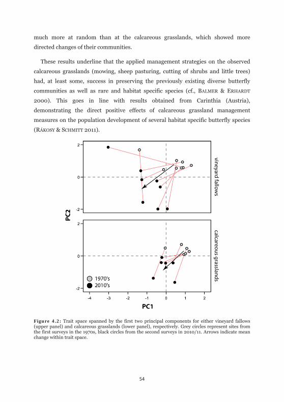
54
much more at random than at the calcareous grasslands, which showed more
directed changes of their communities.
These results underline that the applied management strategies on the observed
calcareous grasslands (mowing, sheep pasturing, cutting of shrubs and little trees)
had, at least some, success in preserving the previously existing diverse butterfly
communities as well as rare and habitat specific species (cf., BALMER & ERHARDT
2000). This goes in line with results obtained from Carinthia (Austria),
demonstrating the direct positive effects of calcareous grassland management
measures on the population development of several habitat specific butterfly species
(RÁKOSY & SCHMITT 2011).
Figure 4.2: Trait space spanned by the first two principal components for either vineyard fallows (upper panel) and calcareous grasslands (lower panel), respectively. Grey circles represent sites from the first surveys in the 1970s, black circles from the second surveys in 2010/11. Arrows indicate mean change within trait space.
55
Nevertheless, the conservation success is not as high as desired: A considerable
number of target species (e.g. Glaucopsyche alexis, Maculinea arion, Hipparchia
semele) disappeared from all study sites, and the rate of species loss at calcareous
grasslands was, in general, only gradually lower than at the unmanaged vineyard
fallows. Thus, the applied management strategies were not able to preserve the status
quo of the 1970s on the calcareous grasslands, but simply prevented natural
succession in a mostly similar way. Therefore, these measures only archived that
community shifts on these sites were somewhat less severe and more in parallel than
on vineyard fallows, which showed much more arbitrary and stochastic community
shifts. Consequently, the management concepts applied at these calcareous
grasslands were not able to outweigh the complex external impacts affecting these
habitats (e.g. influences from adjacent areas, nutrient loads, changing climate), but
had the capability to buffer these negative influences to some extent.
In contrast, the community shifts at the studied vineyard fallows were much more
dynamic, reflecting habitat characteristics and the unbuffered effects resulting from
large and meso-scale environmental changes over the last few decades. Turn-over
rates were considerably higher at the vineyard fallows fostering their stochasticity in
community evolution. The higher habitat connectivity of the vineyard fallows
compared to the highly isolated calcareous grasslands might reinforce these turn-over
dynamics. Consequently, the missing connectivity among calcareous grassland makes
that arbitrary losses of species cannot be compensated by immigration within short
time. Furthermore, gene flow among these isolated populations will be strongly
hampered or even completely blocked so that populations might also disappear due
to the degradation of their gene pools (cf. HABEL & SCHMITT 2012).
In spite of the notable differences between the managed calcareous grasslands and
the unmanaged vineyard fallows, both habitat types show remarkable colinearities in
the ecological traits of the species being lost (Fig. 4.2). These colinearities are unlikely
to be influenced by the differences in management and connectivity, but apparently
are triggered by large-scale environmental factor complexes provoking destructive
impacts on butterfly communities in general, independently from habitat type. As a
result, these impacts cause a similar evolutionary trend towards species poor and
generalist-dominated communities, and thus represent a more holistic problem for
the conservation of biodiversity (e.g., MCKINNEY & LOCKWOOD 1999; WARREN et al.
2001; POLUS et al. 2007).
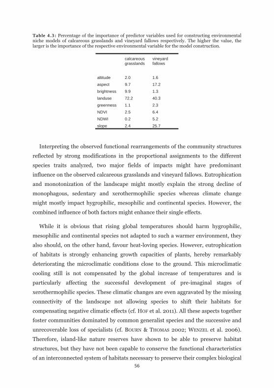
56
Table 4.3: Percentage of the importance of predictor variables used for constructing environmental niche models of calcareous grasslands and vineyard fallows respectively. The higher the value, the larger is the importance of the respective environmental variable for the model construction.
calcareous grasslands
vineyard fallows
altitude 2.0 1.6
aspect 9.7 17.2
brightness 9.9 1.3
landuse 72.2 40.3
greenness 1.1 2.3
NDVI 2.5 6.4
NDWI 0.2 5.2
slope 2.4 25.7
Interpreting the observed functional rearrangements of the community structures
reflected by strong modifications in the proportional assignments to the different
species traits analyzed, two major fields of impacts might have predominant
influence on the observed calcareous grasslands and vineyard fallows. Eutrophication
and monotonization of the landscape might mostly explain the strong decline of
monophagous, sedentary and xerothermophilic species whereas climate change
might mostly impact hygrophilic, mesophilic and continental species. However, the
combined influence of both factors might enhance their single effects.
While it is obvious that rising global temperatures should harm hygrophilic,
mesophilic and continental species not adapted to such a warmer environment, they
also should, on the other hand, favour heat-loving species. However, eutrophication
of habitats is strongly enhancing growth capacities of plants, hereby remarkably
deteriorating the microclimatic conditions close to the ground. This microclimatic
cooling still is not compensated by the global increase of temperatures and is
particularly affecting the successful development of pre-imaginal stages of
xerothermophilic species. These climatic changes are even aggravated by the missing
connectivity of the landscape not allowing species to shift their habitats for
compensating negative climatic effects (cf. HOF et al. 2011). All these aspects together
foster communities dominated by common generalist species and the successive and
unrecoverable loss of specialists (cf. BOURN & THOMAS 2002; WENZEL et al. 2006).
Therefore, island-like nature reserves have shown to be able to preserve habitat
structures, but they have not been capable to conserve the functional characteristics
of an interconnected system of habitats necessary to preserve their complex biological

57
diversity. Without adjustments in nature conservation strategies and considerably
enhanced efforts in enlarging and connecting high quality habitats, the future
perspectives cannot be seen more optimistic.

58

59
CHAPTER 5
Coupling satellite data with species distribution and
connectivity models as a tool for environmental management
and planning in matrix-sensitive species
“We cannot solve our problems with the same thinking we used when we created them.”
ALBERT EINSTEIN

60
This chapter has been submitted to Environmental Management
The work was conducted in collaboration with ANNA F. CORD from the Helmholtz Centre for Environmental Research, as well as SWEN NEKUM and DENNIS RÖDDER from the Zoological Researchmuseum Koenig.
61
Introduction
Climate change and continuing habitat loss through human land-use are currently
considered as major threats for global biodiversity (BELLARD et al. 2012; DEVICTOR et
al. 2012). Although not fully understood, some authors (e.g., HOF et al. 2011) assume
synergistic effects between both processes could lead to an even more dramatic loss
of biodiversity than predicted by studies, focusing on the effects of climate change
alone (PARMESAN & YOHE 2003; THOMAS et al. 2004). Habitat loss and fragmentation
might have serious consequences on demographic dynamics (FAHRING 2003),
metapopulation structure (HANSKI 1998) and the genetic setup of populations
(TEMPLETON et al. 1990; KEYGHOBADI 2007) by hampering the exchange of individuals
between populations. This may lead to a loss of genetic variation (e.g., HABEL &
SCHMITT 2012), potentially resulting in an increase of inbreeding depression (e.g.,
ANDERSEN et al. 2004; ZACHOS et al. 2007) and can ultimately threaten isolated
populations with extinction (e.g., PETTERSON 1985). Therefore, detailed information
on how populations are connected in the landscape is pivotal in guiding more
effective and sustainable conservation measures.
Even though the importance of habitat connectivity has been recognized by both,
researchers and nature conservationists (HALE et al. 2001; GILBERT-NORTON et al.
2010), habitat loss is still accelerating as a consequence of human activities across
different spatial scales and is a major threat for biodiversity (FISCHER & LINDENMAYER
2007). Paying special attention to habitat connectivity during the planning process
can help safeguard the ecological coherence (sensu Habitat Directive; COUNCIL OF THE
EUROPEAN COMMISSION 1992) of an entire region and assist to avoid negative
cumulative effects that might derive from different planning efforts in the same
region (MANDELIK et al. 2005; THERIVEL & ROSS 2007; CANTER & ROSS 2010; DUINKER
et al. 2013). Even though Environmental Impact Assessments (EIAs) aim to assess
such negative environmental effects from infrastructure and other developments, an
evaluation of connective elements is often neglected (GENELETTI 2006). While high
standards regarding the legal basis for EIAs are already realized in many countries,
their application and implementation pose significant challenges. These are due to
time and financial constraints during EIA preparation, which are often accompanied
by controversial political and public debates (CALDWELL 1991; DICKERSON &
MONTGOMERY 1993; DE SMEDT 2010). As a consequence, it is hardly ever possible to
62
provide enough resources for surveys that sufficiently expand the target region
beyond the finite area implemented in an EIA, which allows for an assessment of
potential connectivity between populations of species of special conservation
concern. In most cases, planned developments might affect smaller fragments of a
previously larger, interconnected population (hereafter called the local population) or
even just connective elements between permanently colonized habitat patches. For
planning offices who normally conduct EIAs for specific developments, identifying or
bounding the local population during the evaluation process of the affected habitat
fragments therefore remains a great challenge.
Over the past decades, we have witnessed a tremendous increase in tools and
environmental datasets that can support EIA procedures. These include geographic
information systems (GIS) which have become increasingly important as a useful tool
in environmental and urban planning for more than three decades now (SCHALLER
1990; MAGUIRE 1991; BURROUGH & MCDONNELL 1998; MORRIS & THERIVEL 2001).
Today, GIS techniques have become crucial to visualize mapping results of EIAs and
the underlying structural measures and allows for the integration of metapopulation
theory (HANSKI 1994; 1998) into applications useful for conservation and
environmental planning (NICHOLSON & OVASKAINEN 2009). A further consequence to
the spread of GIS techniques is that the decision-making process for many more
aspects in conservation is becoming more and more spatially explicit, such as the
design of reserve networks (WILSON et al. 2009) or species-specific conservation
management (e.g., RHODES et al. 2006; RÖDDER et al. 2010). Species distribution
models (SDMs) have emerged as one of these new spatially explicit tools. Originally
developed to work on biogeography-related questions on a macro-ecological scale,
they have since been applied in a wide range of ecological disciplines (FRANKLIN
2009; PETERSON et al. 2011). Despite this frequent use in many disciplines, including
conservation biology, there are few academic studies that give special emphasis to the
conservation decision process (GUISAN et al. 2013) and for EIAs in particular
(GONTIER 2006). Due to this lack of scientific guidance on how novel GIS-based
techniques (including SDMs) could contribute to applied biological conservation,
while considering their limits and methodological challenges (POSSINGHAM et al.
2001; ADDISON et al. 2013; GUISAN et al. 2013), confident use by non-experts is hard
to realize (ADDISON et al. 2013, but see GUILLERA-ARROITA et al. 2015). Taking this
into account, we aim here to provide guidance for the use of SDM techniques, in
63
combination with fine-grained remote sensing data and connectivity models, to
assess the potential connectivity of habitat fragments in highly specialized species
with a strong dependence on habitat structure.
Connectivity models are another set of tools that have emerged from, or with the
help of, GIS applications and benefit from the same developments in theory, data
availability, and computer power over the past decades (e.g., HANSKI 1994; MOILANEN
& NIEMINEN 2002; MCRAE 2008; VOGT et al. 2009; LAITA et al. 2011; MIMET et al.
2013). Connectivity is generally seen as species-specific as it depends on the behavior,
habitat preference, and dispersal propensity of the focal species (JOHNSON & GAINES
1985). A useful metric of connectivity for manager guidance thus needs to make a
very accurate estimation of the species-environment relationships under
consideration of the afore mentioned species traits (FAGAN & CALABRESE 2006).
Connectivity can be hereby broadly categorized into two main categories: structural
and functional connectivity (CROOKS & SANJAYAN 2006). The former strictly focus on
the spatial arrangement of landscape elements in the landscape matrix, while the
latter incorporates some additional information on the species' movement either in
direct (actual connectivity) or indirect (potential connectivity) form (FAGAN &
CALABRESE 2006). It is really important to make these distinctions as data
requirements differ and by this, the informational content a connectivity model can
provide to a manager as well.
The combination of species distribution models, connectivity models and the
underlying fine-scaled environmental datasets into a single framework has several
advantages in the spatially-explicit assessment of population connectivity in matrix-
sensitive species (i.e., species’ movement responses functionally depend on the
structure of the habitat matrix, cf. IMS 1995). Aside from a high applicability of the
single approaches due to already available and easy to handle programs, the main
advantage is that species-specific information on landscape-related habitat suitability
can be combined with an objective parameterization of resistance values—two key
aspects that typically lack in the construction of resistance surfaces (i.e. a GIS-raster
of a hypothesized relationship of certain landscape parameters to species-specific
connectivity; see SPEAR et al. 2010 for a discussion). Therefore, we recommend the
use of SDMs as the first step of a two-step framework together with connectivity
models and refer to this framework in the following as a potential connectivity model
(Fig. 5.1; PCM). The PCM framework offers the possibility to quantify potential
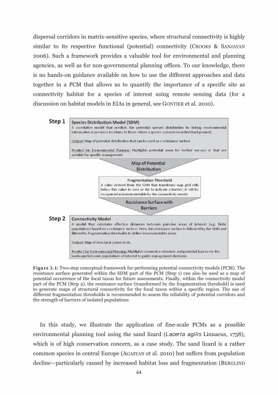
64
dispersal corridors in matrix-sensitive species, where structural connectivity is highly
similar to its respective functional (potential) connectivity (CROOKS & SANJAYAN
2006). Such a framework provides a valuable tool for environmental and planning
agencies, as well as for non-governmental planning offices. To our knowledge, there
is no hands-on guidance available on how to use the different approaches and data
together in a PCM that allows us to quantify the importance of a specific site as
connectivity habitat for a species of interest using remote sensing data (for a
discussion on habitat models in EIAs in general, see GONTIER et al. 2010).
Figure 5.1: Two-step conceptual framework for performing potential connectivity models (PCM). The resistance surface generated within the SDM part of the PCM (Step 1) can also be used as a map of potential occurrence of the focal taxon for future assessments. Finally, within the connectivity model part of the PCM (Step 2), the resistance surface (transformed by the fragmentation threshold) is used to generate maps of structural connectivity for the focal taxon within a specific region. The use of different fragmentation thresholds is recommended to assess the reliability of potential corridors and the strength of barriers of isolated populations
In this study, we illustrate the application of fine-scale PCMs as a possible
environmental planning tool using the sand lizard (Lacerta agilis Linnaeus, 1758),
which is of high conservation concern, as a case study. The sand lizard is a rather
common species in central Europe (AGASYAN et al. 2010) but suffers from population
decline—particularly caused by increased habitat loss and fragmentation (BERGLIND
65
2000; ELLWANGER 2004). Consequently, it has become recognized as a threatened
species and is protected under the EU Habitats Directive (92/43/EEC; ELLWANGER
2004), being listed in Annex IV as a species of community interest. Sand lizards are
sensitive to fine-scale habitat features and often occupy ecotones or secondary
habitats such as railway or road embankments (GLANDT & BISCHOFF 1988) and can
often be considered having a classical metapopulation structure comprising
interlinked habitat patches of different size and quality (BERGLIND 2004). It has been
highlighted, that railways can act as an ideal corridor between suitable habitat
patches (BLANKE 1999), whereas highways mirrored by noise walls may act as an
insurmountable barrier for successful inter-population connectivity in this species
(BLANKE 2010). These characteristics make the sand lizard a highly matrix-sensitive
species. Increasing habitat loss of remnant populations—as a result of anthropogenic
development of the landscape (particularly in rural areas) —make this species an
ideal candidate organism for connectivity assessments. We evaluate the landscape
connectivity amongst different sand lizard populations inhabiting a strongly
urbanized region in Western Germany and are subject to varying fragmentation
intensities and thus metapopulation dynamics. In particular, we conducted
standardized surveys and sample high resolution occurrence records to generate a
map of potential distribution which could be used (1) as prior information for future
mapping efforts of sand lizard populations, and (2) for the evaluation of potential
corridors, highlighting the importance of spatially explicit linkages of connective
habitats between well-known populations.
Material and methods
Study area and data sampling
The study area comprises over 400 km², covering the city of Cologne and
immediate surroundings, located in Western Germany (50.9°N, 7.0°E). Cologne is
Germany’s fourth-largest city and is located within the Rhine-Ruhr Metropolitan
Area. Geographically, the study region can be described as a lowland area, with an
altitudinal range between 35 and 118 m a.s.l.. The area is surrounded by more
mountainous areas (Rhenish Uplands in the south, the High Fens and Eifel in the
west, and the Bergisches Land in the east) while it is connected to other lowland areas
in the north. The Rhine River divides the study region into a western and eastern
part. The area has a long tradition of human land use and has been used for
66
settlements and agriculture for several thousands of years. This has led to a patchy
landscape structure of settlements, arable lands, meadows, shrubs and forests in its
surroundings, as well as densely populated areas intersected by fallows, parks and
gardens within the city of Cologne.
Building on the results of a preliminary survey with the objective of spotting sand
lizard populations and identifying suitable habitat patches, we selected 30 study sites
within the area, covering all known local populations within the city of Cologne, and
further sites of high structural suitability where existence was so far unconfirmed.
Between May and September 2011, each site was surveyed for 60 minutes on five
different dates, under favorable weather conditions, along standardized transects
with a length of approximately 250 m, following the guidelines of ELLWANGER (2004).
The location of each sand lizard sighting was accurately measured using a GPS device
(Garmin Etrex Vista HCx), resulting in a total of 1,204 occurrence locations of 22
populations (no sand lizard populations were detected at eight of the sites). Condition
status of each population was evaluated following a standardized ABC evaluation
scheme for monitoring species after Art. 11 and 17 of the Habitat Directive in
Germany (ELLWANGER 2004; SCHNITTER et al. 2006; LANUV NRW 2010). This allows
for an easy, transparent and comparable evaluation of the species’ condition status by
allocating classes A (excellent), B (good) or C (poor) for different aspects, such as
population status, habitat quality and threats, as well as a summary classification for
the whole population. For example, an excellent population (class A) is characterized
by the sighting of > 20 individuals per hour of all ages and sexes found during the
visits along a 250 m transect (ELLWANGER 2004), a habitat of superior quality with a
fine-scale structuring and a close connection to neighboring populations within a 500
m range as well as less risk for threats such as presence of feral cats, no (or few)
streets or paths as well as > 1,000 m to the next urban areas. In contrast, a poor
population (class C) is characterized by less than 10 individuals per hour without any
young or subadult individuals, a habitat of low structural quality without adequate
places for reproduction, neighboring populations >1 kilometer apart and severe
threats such as cats, many paths or streets and a close distance to urbanized areas.
Class B would be located in between A and C in its respective conditions.
Satellite data
67
Fine-scale satellite data was obtained from the NASA Landsat 5-TM satellite
archive via the USGS Global Visualization Viewer (http://glovis.usgs.gov/; accessed
on September 10th, 2011). We obtained three nearly cloud-free Landsat 5 scenes
acquired on August 4th, 2009, June 4th, 2010, and October, 10th 2010, with a grain
size of 30 m x 30 m. The scenes were selected based to cover several months during
the main activity stages of the sand lizard, which ranges from April to October
including the main season of dispersal of the offspring (August – October). This
allows us to account for phenological changes in vegetation throughout the activity
season which are important to characterize the sand lizard's habitat (GLANDT &
BISCHOFF 1988). To minimize possible confounding effects and artifacts of the scenes
due to past developments, we focus on images that were captured not more than two
years prior our sampling. The scenes covered the southern part of Northrhine-
Westphalia, including southerly adjacent parts of Rhineland-Palatinate. All datasets
were radiometrically corrected using the Empirical Line Correction method (ROBERTS
et al. 1985) as implemented in ENVI version 4.5 (ITT 2008), based on bright (urban)
and dark (water) reference spectra, extracted from the respective images. Each scene
comprised of seven raw spectral bands, each representing a special part of the
electromagnetic spectrum. From the spectral bands 1-5 and 7, we calculated a several
spectral indices, namely the Normalized Difference Vegetation Index (NDVI) as well
as greenness, brightness, and moisture according to the Tasseled Cap Transformation
(CRIST & CICONE 1984). Furthermore, effective at-satellite temperature was obtained
from spectral radiance values of band 6 using the Landsat 5-TM Thermal Band
Calibration Constants (NASA, 2002). Since multi-collinearity among the predictors
hampers the interpretability of species-environment relationships (HEIKKINEN et al.
2006; DORMANN et al. 2013), we estimated the pairwise cross-correlation among the
33 remotely-sensed environmental layers (including 6 bands and 5 indices for 3 time
steps). We retained 18 low intercorrelated (R² < 0.75) predictors entering the SDM,
which we assumed to be best suited for characterizing the micro habitats of sand
lizards in terms of vegetation structure, density and water stress, as well as
temperature (see also GLANDT & BISCHOFF 1988). We thus did not give a priori favor
to calculated indices over raw bands as raw bands might include important variation
that might get lost in the tasseled cap transformation. Table 5.1 shows the used bands
and gives an ecological explanation of their meaning.
Table 5.1: Details of the spectral bands covered by Landsat and indices calculated based upon them. Variables finally included into the SDM after accounting for multi-collinearity are marked with an x.
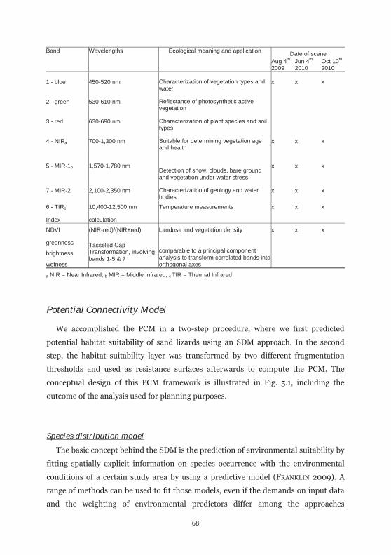
68
Band Wavelengths Ecological meaning and application Date of sceneAug 4th 2009
Jun 4th 2010
Oct 10th 2010
1 - blue 450-520 nm Characterization of vegetation types and water
x x x
2 - green 530-610 nm Reflectance of photosynthetic active vegetation
3 - red 630-690 nm Characterization of plant species and soil types
4 - NIRa 700-1,300 nm Suitable for determining vegetation age and health
x x x
5 - MIR-1b 1,570-1,780 nm Detection of snow, clouds, bare ground and vegetation under water stress
x x x
7 - MIR-2 2,100-2,350 nm Characterization of geology and water bodies
x x x
6 - TIRc 10,400-12,500 nm Temperature measurements x x x
Index calculation
NDVI (NIR-red)/(NIR+red) Landuse and vegetation density x x x
greenness Tasseled Cap Transformation, involving bands 1-5 & 7
comparable to a principal component analysis to transform correlated bands into orthogonal axes
brightness
wetness
a NIR = Near Infrared; b MIR = Middle Infrared; c TIR = Thermal Infrared
Potential Connectivity Model
We accomplished the PCM in a two-step procedure, where we first predicted
potential habitat suitability of sand lizards using an SDM approach. In the second
step, the habitat suitability layer was transformed by two different fragmentation
thresholds and used as resistance surfaces afterwards to compute the PCM. The
conceptual design of this PCM framework is illustrated in Fig. 5.1, including the
outcome of the analysis used for planning purposes.
Species distribution model
The basic concept behind the SDM is the prediction of environmental suitability by
fitting spatially explicit information on species occurrence with the environmental
conditions of a certain study area by using a predictive model (FRANKLIN 2009). A
range of methods can be used to fit those models, even if the demands on input data
and the weighting of environmental predictors differ among the approaches

69
(FRANKLIN 2009; PETERSON et al. 2011). For SDM development, we used the open
source software, MAXENT 3.3.3e (PHILLIPS et al. 2006; PHILLIPS & DUDÍK 2008; ELITH
et al. 2011), which has frequently outperformed other approaches, even under
difficult circumstances (e.g., ELITH et al. 2006; HERNANDEZ et al. 2006; WISZ et al.
2008). MAXENT is a method focused on presence-only data and contrasts the
environmental conditions at the presence records to a set of background locations
where presence is unknown (i.e., background points; a detailed explanation of this
method relevant for users is given in ELITH et al. 2011 and MEROW et al. 2013). Given
our highly standardized sampling scheme including a high coverage of the majority of
populations within the study area we used the entire set of records (n = 1,204) to
account for different population sizes at the certain patches, which was mentioned to
be an ideal prerequisite in presence-only models (FITHIAN & HASTIE 2013; MEROW et
al. 2013). We randomly selected 10,000 background records from a rectangular area
surrounding the city of Cologne, as the species potentially inhabits the whole region.
We applied the standard settings of Maxent with a logistic output format, randomly
splitting the entire set of species records in a bootstrap approach into 70% used for
SDM training, and 30% for testing. This procedure was repeated 100 times and the
average prediction per grid cell was used for further processing. The resulting map of
potential distribution can be used as a resistance surface, were high values along the
logistic distribution indicate low resistance after accounting for barriers (i.e. applying
fragmentation thresholds, see Fig. 5.1 and next section), to calculate effective
resistances between the investigated populations.
Fragmentation thresholds
To assess the sensitivity of the PCM, we modified the resistance surface based on
two different fragmentation thresholds. Values of the resistance surface below the
specific fragmentation threshold were set as absolute barriers for the connectivity
model (see next section), whereas the other values remain as they are (i.e., bounded
between the applied fragmentation threshold and 1). This is a crucial step in
evaluating the sensitivity of the potential corridors, as a continuous surface without
absolute barriers will lead to unrealistic potential movement paths in the landscape
(e.g., the connectivity model might mistakenly connect patches across constructed
areas or large water surfaces with very low suitability values). By comparing a more
sensitive threshold against a more conservative one, regions of stable connective
70
predictions could be classified with a higher priority for planning issues, rather than
regions where connective predictions are fluctuating. In turn, areas of high
fluctuation in corridor predictability could be used for targeted compensation or
restoration actions. In the selection of the two fragmentation thresholds we choose
two different criteria, one focusing on the underlying occurrence records used to
compute the SDM, and another based on the fitted logistic function of the SDM, to
tackle different sources of uncertainty. In the former, we assume that 5% of the
records used to build the SDM were situated at the edge of the species’ source habitat
(i.e., located close to the edge of the habitat patch, where the environmental
information of the respective grid cell might be strongly influenced by surrounding
unsuitable habitat) or even outside of it. This threshold (in the following referred to
as 5th percentile occurrence threshold) highlights only those regions with strong
structural connectivity between populations and can be seen rather sensitive. We
defined the second threshold as the relative probability of habitat suitability at an
occurrence record that had the next largest resistance value, compared to the one-
sided 95% confidence limit of the logistic distribution (i.e., a value > 0.05 of the
logistic distribution; in the following referred to as 5% logistic threshold). In our case,
the latter threshold matches the logistic model output at bridges crossing the Rhine
River, a major natural barrier in our study area. In consequence, the 5% logistic
threshold gives a stronger emphasis to areas with a weaker structural connectivity
and can be seen as conservative in comparison to the 5th percentile occurrence
threshold. Although habitat suitability might be low, these habitat patches can still
serve as stepping stones, providing a connection to other potential populations not
discovered in this assessment.
Connectivity model
Connectivity models allow the assessment of ecological coherence among locations
of a given resistance surface by identifying barriers or corridors of functional
exchange (e.g. in terms of individuals or genotypes). These tools become increasingly
available and are of high relevance for conservation decision-making and
environmental planning (CROOKS & SANJAYAN 2006). Approaches that consider
multiple paths across the whole landscape add great value to our understanding of
habitat connectivity compared to the more classical approaches such as least-cost
path models, which focus on a single habitat corridor that minimizes the costs
71
between two sites (DRIEZEN et al. 2007; MCRAE & BEIER 2007; SAWYER et al. 2011).
Among those approaches, connectivity measures based on electrical circuit theory are
gaining much attraction in situations where random walk can be assumed (DOYLE &
SNELL 1984; CHANDRA et al. 1997; MCRAE et al. 2008). This concept has been
successfully shown to outperform other connectivity measures in a landscape-genetic
framework (MCRAE & BEIER 2007). A detailed ecological description of connectivity
measures underlying the circuit theoretic framework can be found in MCRAE et al.
(2008). Briefly, following Ohm’s law, circuit theory predicts the current flow from a
set of nodes (i.e., grid cells of a two-dimensional GIS raster) along resistors (i.e.,
functional connections between the nodes that conduct current). The higher the
resistance at the resistors, the lower the current flow is between the nodes.
Additionally, both number and spatial configuration of the resistors influence current
flow. The effective resistance (measured in ohm) can thus be seen as a measure of
isolation between pairs of cells (for instance the isolation between populations or
individuals) in a raster grid representing the landscape of interest. From this, this
concept is similar to the ecological concept of effective distances, but in this case,
measured by incorporating alternative pathways rather than a single least cost path.
For this purpose, CIRCUITSCAPE 3.5.4 (MCRAE & BEIER 2007; MCRAE et al. 2008)
was used. In the Circuitscape analyses, a pairwise connection scheme was applied
based on focal regions defined by the 22 surveyed sand lizard populations within the
study area. Focal regions represent a lumped set of nodes where the species was
found and that is not intersected by the surrounding habitat matrix. Grid cell
connections were allowed in eight directions (i.e., including adjacent nodes in
horizontal or vertical directions, as well as diagonal neighbor nodes; Queen’s case).
These settings were applied to the analysis of both resistance surfaces modified by the
respective fragmentation thresholds.
72
Results
Estimated condition status of Colognes’ sand lizard populations based on field observations
Following the recommendations of SCHNITTER et al. (2006) for ascertaining the
condition status of sand lizard populations based on the count frequency of
individuals observed along a transect, five of the 22 investigated populations were
considered to be residing in excellent conditions (i.e., > 20 individuals found).
Furthermore, nine populations were estimated to be in good conditions (i.e., 10 – 20
individuals found), while the remaining eight populations need to be considered as
residing in poor or bad conditions (i.e., < 10 individuals found; Table 5.2). Also taking
into account the general habitat conditions and recent threat factors (LANUV NRW
2010), the same five investigated lizard populations were assessed as status A
(excellent preservation status), whereas eleven populations were assigned to status B
(good preservation status). The remaining six populations were considered to reside
in status C (poor to bad preservation status; Table 5.2).
Distribution of potential habitats
The performance of the SDM was excellent, with mean AUCtest of 0.899 (sd ±
0.006). Temperature-related variables of the satellite data acquired in August 2009
and June 2010 had, on average, the highest variable contribution (20.7 % and 18.3 %,
respectively) followed by the middle-infrared-1 layer of June 2010 (15.0 %; Table
5.3). These predictors highlighted typically dry and hot sites as key habitats for this
species, which is known to be of high importance for this species (GLANDT & BISCHOFF
1988). This finding is further supported by our field data that highlight the amount of
dead wood, open-land vegetation, railway sidings, as well as diverse materials of
anthropogenic origin (i.e., garden waste or demolition materials), as typical habitat
features of adult sand lizards at the study plots. As derived from the SDM, the
potential distribution of sand lizards in Cologne is increasingly patchy in the more
central und urbanized parts of the city (Fig. 5.2a). Protected heath- and shrubland, as
well as industrial wastelands, may therefore serve as the best potential habitats for
sand lizards in this area. Nevertheless, habitats exposed to a strong anthropogenic
influence such as the border areas of surface mining regions, railways and their
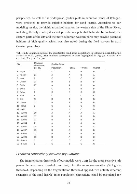
73
peripheries, as well as the widespread garden plots in suburban zones of Cologne,
were predicted to provide suitable habitats for sand lizards. According to our
modeling results, the highly urbanized area on the western side of the Rhine River,
including the city centre, does not provide any potential habitats. In contrast, the
eastern parts of the city and the more suburban western parts may provide potential
habitats of high quality, which was also noted during the field surveys in 2011
(Nekum pers. obs.).
Table 5.2: Condition status of the investigated sand lizard populations in Cologne in 2011, following SCHNITTER et al. (2006). Site numbers correspond to those highlighted in Fig. 5.2. Classes: A = excellent, B = good, C = poor.
Site Maximum abundance per day
Quality Class
Population Habitat Threats Overall
1 - Bayer 7 C B B B
2 - Knobw 21 A A B A
3 - Horn 9 C C C C
4 - Duenn 13 B B B B
5 - Dellh 27 A A B A
6 - Scha 7 C B B B
7 - Poho 5 C C C C
8 - Rad 4 C C C C
9 - Joli 16 B B B B
10 - Grem 12 B B B B
11 - Imlue 2 C C C C
12 - Leih 11 B B C B
13 - WH08 29 A A A A
14 - WH06 17 B A B B
15 - WH05 11 B B B B
16 - WH04 21 A A A A
17 - WH01 28 A A B A
18 - WH07 15 B A B B
19 - WH02 12 B B B B
20 - WH03 13 B A B B
21 - Boeck 3 C C C C
22 - S-Aue 2 C B C C
Predicted connectivity between populations
The fragmentation thresholds of our models were 0.131 for the more sensitive 5th
percentile occurrence threshold and 0.071 for the more conservative 5% logistic
threshold. Depending on the fragmentation threshold applied, two notably different
scenarios of the sand lizards’ inter-population connectivity could be postulated for
74
predicting different proportions of the study area as suitable habitat (Fig. 5.2a).
Figures 5.2b and 5.2c show the differences between the investigated populations for a
detailed area located in the northeastern part of the city when applying the two
different fragmentation thresholds. Direct comparisons highlight: (1) a conservative
connectivity network between populations one, two and four; (2) a very sensitive
connectivity network towards populations three and five; and (3) a strong isolation
under both thresholds for population six.
Discussion
Today's practice in urban and environmental planning and management often
lacks quantitative assessments of potential corridors that connect populations of
species with a high conservation concern. Herein, we introduced a PCM based on
fine-scale multispectral satellite data to assess the potential connectivity using sand
lizards as a case study.
Applicability of the approach
By using different fragmentation thresholds as reliability measures of the potential
corridors (ANDRÉN 1994; see also METZGER & DÉCAMPS 1997), we were able to
highlight areas of strong connectivity, persistent isolation or of unstable connective
networks (Fig. 5.2 b,c) with different implications for planning purposes and
metapopulation dynamics. In particular, populations one, two and four appear to be
located within a reasonably stable landscape matrix with structural elements
connecting the populations into a viable metapopulation network, irrespective of the
fragmentation threshold used. This conservative connectivity matrix should be
preserved and considered when planning projects in this area become acute (i.e., by
safeguarding connective elements). Due to the spatial configuration of available
habitat patches, along with the (effective) distance among them, stochastic extinction
events at certain patches can be balanced by migration events within a larger
interconnected metapopulation (HANSKI 1994; MOILANEN & HANSKI 1998) which
might be also beneficial under expected climate change (NICHOLSON & OVASKAINEN
2009). In contrast, population six showed a strong and consistent isolation from all
other populations in this area for both threshold scenarios. Here, a closer look at the
viability and genetic setup of the population would be beneficial to finally evaluate its
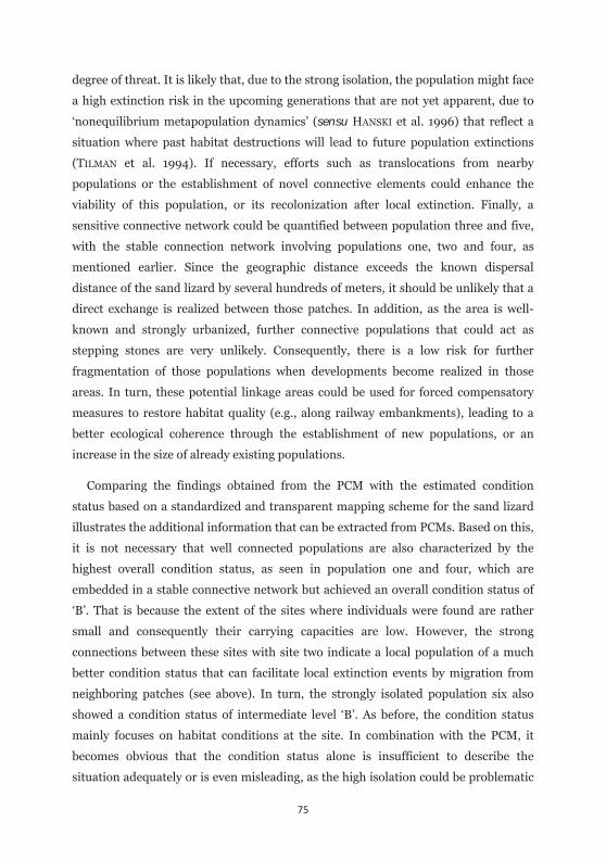
75
degree of threat. It is likely that, due to the strong isolation, the population might face
a high extinction risk in the upcoming generations that are not yet apparent, due to
‘nonequilibrium metapopulation dynamics’ (sensu HANSKI et al. 1996) that reflect a
situation where past habitat destructions will lead to future population extinctions
(TILMAN et al. 1994). If necessary, efforts such as translocations from nearby
populations or the establishment of novel connective elements could enhance the
viability of this population, or its recolonization after local extinction. Finally, a
sensitive connective network could be quantified between population three and five,
with the stable connection network involving populations one, two and four, as
mentioned earlier. Since the geographic distance exceeds the known dispersal
distance of the sand lizard by several hundreds of meters, it should be unlikely that a
direct exchange is realized between those patches. In addition, as the area is well-
known and strongly urbanized, further connective populations that could act as
stepping stones are very unlikely. Consequently, there is a low risk for further
fragmentation of those populations when developments become realized in those
areas. In turn, these potential linkage areas could be used for forced compensatory
measures to restore habitat quality (e.g., along railway embankments), leading to a
better ecological coherence through the establishment of new populations, or an
increase in the size of already existing populations.
Comparing the findings obtained from the PCM with the estimated condition
status based on a standardized and transparent mapping scheme for the sand lizard
illustrates the additional information that can be extracted from PCMs. Based on this,
it is not necessary that well connected populations are also characterized by the
highest overall condition status, as seen in population one and four, which are
embedded in a stable connective network but achieved an overall condition status of
‘B’. That is because the extent of the sites where individuals were found are rather
small and consequently their carrying capacities are low. However, the strong
connections between these sites with site two indicate a local population of a much
better condition status that can facilitate local extinction events by migration from
neighboring patches (see above). In turn, the strongly isolated population six also
showed a condition status of intermediate level ‘B’. As before, the condition status
mainly focuses on habitat conditions at the site. In combination with the PCM, it
becomes obvious that the condition status alone is insufficient to describe the
situation adequately or is even misleading, as the high isolation could be problematic
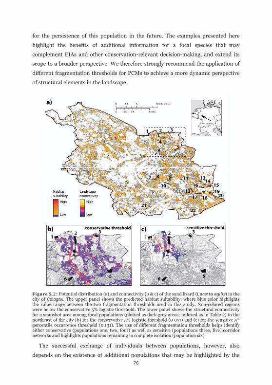
76
for the persistence of this population in the future. The examples presented here
highlight the benefits of additional information for a focal species that may
complement EIAs and other conservation-relevant decision-making, and extend its
scope to a broader perspective. We therefore strongly recommend the application of
different fragmentation thresholds for PCMs to achieve a more dynamic perspective
of structural elements in the landscape.
Figure 5.2: Potential distribution (a) and connectivity (b & c) of the sand lizard (Lacerta agilis) in the city of Cologne. The upper panel shows the predicted habitat suitability, where blue color highlights the value range between the two fragmentation thresholds used in this study. Non-colored regions were below the conservative 5% logistic threshold. The lower panel shows the structural connectivity for a snapshot area among focal populations (plotted as dark grey areas; indexed as in Table 2) in the northeast of the city (b) for the conservative 5% logistic threshold (0.071) and (c) for the sensitive 5th percentile occurrence threshold (0.131). The use of different fragmentation thresholds helps identify either conservative (populations one, two, four) as well as sensitive (populations three, five) corridor networks and highlights populations remaining in complete isolation (population six).
The successful exchange of individuals between populations, however, also
depends on the existence of additional populations that may be highlighted by the
77
habitat suitability map. Due to the restricted dispersal propensity of our focal species,
structural connective elements may become irrelevant when existing stepping stones
(i.e., additional populations) are missing, which would ensure the ecological
coherence in the metapopulation. Therefore, the first step is to assess the occurrence
of potential additional populations identified by the habitat suitability map.
Depending on the large distance among the different populations, we consider the
potential corridors important for inter-population exchange in the sand lizard
example.
Table 5.3: Variable importance as measured with three different procedures in Maxent. For each measure, the mean and the respective sd is shown. Values of the most important variables in either measure are highlighted in bold. Variable names are coded as follows for month_year_spectral band/index as denoted in Table 5.1.
Variable contribution
permutation importance Jackknife tests of variable importance
AUCtest without ... AUCtest with only ...
10_10_blue 0.55 0.320 1.05 0.446 0.898 0.006 0.634 0.013 10_10_MIR-1 5.17 1.264 6.87 1.387 0.897 0.006 0.679 0.013 10_10_MIR-2 0.77 0.303 3.37 1.179 0.897 0.006 0.611 0.013 10_10_NDVI 0.96 0.646 0.98 0.637 0.899 0.006 0.688 0.013 10_10_NIR 2.12 1.035 2.49 0.951 0.899 0.006 0.693 0.012 10_10_TIR 5.85 0.936 7.15 1.629 0.896 0.006 0.682 0.012 6_10_blue 1.03 0.520 2.11 0.937 0.899 0.006 0.659 0.012 6_10_MIR-1 14.98 2.106 17.56 3.634 0.896 0.006 0.696 0.012 6_10_MIR-2 2.22 1.658 3.66 1.464 0.898 0.006 0.655 0.013 6_10_NDVI 6.29 2.078 4.18 1.531 0.898 0.006 0.709 0.012 6_10_NIR 5.88 1.442 6.97 1.821 0.897 0.006 0.699 0.012 6_10_TIR 18.29 2.945 15.01 2.572 0.893 0.006 0.757 0.011
8_09_blue 4.60 1.294 5.09 1.287 0.897 0.006 0.685 0.011 8_09_MIR-1 2.50 0.667 2.58 0.946 0.898 0.006 0.682 0.012 8_09_MIR-2 2.70 1.099 2.25 0.786 0.898 0.006 0.664 0.011 8_09_NDVI 3.30 1.561 1.56 0.704 0.899 0.006 0.709 0.012 8_09_NIR 2.09 0.791 1.71 0.699 0.899 0.006 0.686 0.011 8_09_TIR 20.70 2.696 15.40 3.460 0.896 0.006 0.761 0.011
A final aspect concerns the vulnerability of the populations due to climate change.
Temperature is expected to increase by 1.6-3.8°C in Germany by 2080 (ZEBISCH et al.
2005). As temperature is an inherent factor for sand lizard’s distribution, an increase
of this magnitude could lead to local extinctions of populations and, consequently, a
shift of current local distribution patterns. Reachable neighboring populations are
therefore mandatory for a successful persistence of the metapopulation under climate
78
change. However, this would raise the need for more flexibility in reserve designs and
conservation planning as shown for other lizard species (RÖDDER & SCHULTE 2010).
Data requirements and limitations for further applications
The applicability of the approach strongly depends on the species of interest. As
mentioned throughout the manuscript, matrix-sensitive species are required for this
approach as in these species functional connectivity closely matches structural
connectivity and allows a direct link between habitat suitability and landscape
connectivity. For instance, birds normally strongly diverge between functional und
structural connectivity due to their high mobility and are therefore not suitable to this
approach. However, matrix-sensitive species might be ideal surrogates for
connectivity (so called umbrella or focal species; LAMBECK 1997; ROBERGE &
ANGELSTAM 2004), as management implications based upon such species should also
beneficial for other co-occurring species that share similar ecological demands (e.g.,
VOS et al. 2001) or who are functionally less bounded by the habitat structure, so
further habitat will be preserved. Another approach might be to select different
suitable species and independently conduct PCMs for each of them and overlay
output maps of potential connectivity for a cumulative assessment of connectivity for
an entire community of matrix-sensitive species in a specific region that can be used
to guide site prioritization for further management. This can be advantageous when
EIA studies need to assess a wider range of species in the same area that diverge in
habitat demands.
Once a species or a set of species for a connectivity assessment has been chosen,
the next step is the selection of appropriate environmental predictors and the
compilation of species records. The number and spatial distribution of occurrence
records is very important, as the SDM algorithms demand a specific minimum
number of locations for model training. The MAXENT algorithm used here has been
proven to provide good results, even though the number of occurrence records is low
(HERNANDEZ et al. 2006; PEARSON et al. 2007; WISZ et al. 2008). However, the
minimum number of species records also depends on the diversity of occupied
habitats of the species. SDMs trained with few species records might already provide
reasonable results if the target species occupies a narrow ecological niche and thus
has very specific habitat demands. The development of an SDM for a generalist
79
species, however, would require a higher number of species records to cover the full
variability of its occupied habitat types.
The selection of suitable predictor variables is a crucial step in SDM development.
It has been shown that SDMs perform best based on predictors with a high biological
relevance for the target species (RÖDDER et al. 2009; RÖDDER & LÖTTERS 2010). In the
sand lizard example, we focused on variables capturing habitat features during the
summer months, when the species is reproducing and dispersal is most likely. Here,
temperature variables of the summer months June and August contributed most to
the model, followed by middle infrared reflectance (MIR-1) in June (Table 5.3), which
highlights dry areas and bare grounds (Table 5.1). However, the biological
importance of predictors may vary among different taxa and geographic areas.
Our example of the sand lizards in Cologne highlights another issue: the extent
to which the interpretation of output maps is ecologically meaningful. In this study,
we focused on the assessment of connectivity among populations that occur on the
eastern side of the Rhine River, which serves as a natural barrier. As only very few
occurrences from the western part of the city were recorded in the field and
information about existing populations is therefore largely lacking, assessments of
habitat connectivity in this area are highly speculative. PCMs are hence most
informative in areas where the majority of existing populations is known and thus
available to train the connectivity model. In addition, connectivity assessments ignore
populations that are located just outside this area of interest. Consequently, either the
outer margins of a particular study site have to be excluded from a quantitative
evaluation or additional populations located outside the area of interest have to be
included in the analysis.
Conclusion
Despite some limitations, the application of PCMs for matrix-sensitive species of
high conservation concern may be a helpful tool to quantify potential connectivity
areas that can act as an additional source of information for urban and environmental
planning. Adaptations of this method should be easily attainable, depending on the
increasing availability of fine-scale environmental data for any matrix-sensitive
species (e.g., provided by the RapidEye mission and the prospective launch of the
Sentinel series, which will allow assessments on even finer spatial scales) and could

80
also support metapopulation models (MOILANEN & HANSKI 1998) suitable for
conservation planning (NICHOLSON & OVASKAINEN 2009) by including the effective
distances among habitat patches as measured by the PCM instead of Euclidean
distances (MOILANEN & HANSKI 2006; NICHOLSON & OVASKAINEN 2009). Therefore,
we strongly recommend the careful use of this tool in conjunction with conservation-
related decision-making procedures such as EIAs. This tool will be a step towards to
overcome recent shortcomings in the planning process that mainly emphasize the
value of reproduction sites and attach less importance to inter-population
connectivity for maintaining healthy and viable local populations.

81

82

83
PART BPCM’S IN LANDSCAPE GENETICS

84

85
CHAPTER 6
Comparative landscape genetics of three closely related
sympatric Hesperid butterflies with diverging ecological traits
“Doing science, particularly the synthesis of disparate ideas, is not as arcane as it is often made out to be. Discipline and taste play a vital role, but the activity is familiar to anyone who has made some effort to be creative”
JOHN HENRY HOLLAND

86
This chapter has been published in PLoS one 9: e106526
The work was conducted in collaboration with NIKO BALKENHOL from the Wildlife Science Department, University of Göttingen, KATHARINA J FILZ from the Biogeography Department, University of Trier, JAN C HABEL from the Department of Ecology and Ecosystemmanagement at the TU Munich and DENNIS RÖDDER from the Zoological Researchmuseum Koenig.

87
Introduction
In the theory of island biogeography, MCARTHUR & WILSON (1967) predicted the
evolution of biodiversity on islands based on two key factors: habitat size and
isolation. Later, this island based model was adopted to explain population structure
of organisms in mainland ecosystems consisting of habitat patches surrounded by a
semi- or non-permeable matrix. This mainland transformation of the theory of island
biogeography inspired the fundamental paradigm of the metapopulation concept
(LEVINS 1969; HANSKI 1999) and also of the neutral theory in both macroecology and
population genetics (HU et al. 2006; LOMOLINO & BROWN 2009). Ultimately, island
biogeography theory revolutionizes our thinking on habitat fragmentation and
conservation biology (summarized in LAURANCE 2009). Apart from habitat size and
isolation, spatial biodiversity patterns are also influenced by additional factors such
as habitat quality (DENNIS & EALES 1997), intrinsic characteristics of species-specific
dispersal behaviour (CONRADT et al. 2001; VAN DYCK & BAGUETTE 2005) and
ecological tolerance (HABEL et al. 2009a) of species. Importantly, population
responses are highly species-specific, when the quality of the landscape matrix in
between suitable habitat patches is reduced (GOODWIN 2003). This would also have
consequences for global biodiversity (FAHRIG 2003; HOF et al. 2011) and large scale
conservation efforts (SEIFERLING et al. 2012).
Understanding the effects of the landscape matrix on realized dispersal and
functional population connectivity is also a major focus of landscape genetics
(HOLDEREGGER & WAGNER 2008; STORFER et al. 2010; MANEL & HOLDEREGGER 2013).
Incorporating spatial landscape information with population genetic data goes far
beyond the classical analysis of isolation-by-distance (IBD; WRIGHT 1943). Species
respond differently to the landscape, in terms of their dispersal, which ultimately
affects the rates of gene flow among local populations (GOLDBERG & WAITS 2010;
RICHARDSON 2012). While the classical isolation-by-distance approach introduced by
WRIGHT (1943) accounts for the geographic (Euclidean) distance between sampled
populations only, other approaches such as the recently proposed isolation-by-
resistance (IBR) concept (MCRAE 2006) accounts for these species-specific responses
to different landscape components that impede or favor gene-flow across a given
landscape matrix.
88
Many studies assess landscape effects on gene flow in only a single species.
However, to understand how landscape effects on gene flow differ between species,
and to take effective conservation actions, it is important to analyze multiple species
in the same landscape using identical methods (SCHWENK & DONOVAN 2011).
However, past studies comparing different species mostly focused on species that
inhabited comparable habitats, but were taxonomically independent (GOLDBERG &
WAITS 2010; RICHARDSON 2012; POELCHAU & HAMRICK 2012). A different comparative
approach is to analyze landscape genetic relationships in closely related taxa
inhabiting the same landscape. Such a focus on taxonomically related sympatric
species (i.e., congeneric species which have the same or overlapping geographic
ranges, regardless of whether or not they co-occur at the same locality) allows the
assessment of traits that gradually change between the congeners independently from
confounding effects that may arise in relation to different evolutionary histories or
environments, respectively (STEELE et al. 2009; DAWSON 2012). Next to dispersal
propensity, niche breadth (i.e. the degree of specialization on specific habitat traits) is
a very important trait in this respect, as it is directly associated with the available
habitat within a landscape.
Generalist species can be found in a broader variety of ecosystems, showing higher
abundances and broader spatial distributions. In contrast, specialist species
demanding certain habitat conditions are often geographically restricted to specific
habitats and usually occur in lower local abundances (HABEL et al. 2013). Apart from
ecological demands, connectivity among local populations is further influenced by the
dispersal propensity of species. Typically, sedentary species are mostly characterized
by rather limited individual exchange compared to species with strong dispersal
behavior. These ecological and behavioral traits also affect the genetic structure of
generalist versus specialist species (HABEL et al. 2009a; 2013; HABEL & SCHMITT
2012). Organisms with specific habitat demands and restricted dispersal behavior
should generally be characterized by low gene flow resulting in strong genetic
differentiation. In contrast, species with weaker habitat specificity and higher
dispersal propensity should show increased levels of gene flow, leading to a lack of
genetic differentiation. Importantly, landscape influences on gene flow and resulting
genetic patterns could also differ between generalist and specialist species inhabiting
the same landscape.
89
In this study, we present a comparative landscape genetic analysis involving three
closely-related butterfly species, to assess the impact of landscape parameters (i.e.,
land use, topography and climatic conditions) on the genetic structure of sympatric
species with different ecological traits. We re-analyzed a molecular dataset taken
from a previous study (LOUY et al. 2007), where landscape effects were previously
ignored, involving three congeneric, but ecologically divergent skipper species of the
genus Thymelicus (HUBNER 1890). The three species include the generalist T. lineola,
which occurs in high abundances and shows strong dispersal propensity; the
specialist T. acteon which is sedentary and occurs restricted to specific habitats; and
T. sylvestris, which lies in between these two extremes in terms of habitat specificity
and dispersal abilities. Using these three species, we (i) investigate the impact of
ecological traits on species-specific functional landscape connectivity and (ii)
determine the overall relevance of landscape characteristics for connectivity in each
species, as well as the individual importance of topography, climatic conditions and
land-use parameters. We hypothesized that species-specific landscape effects on gene
flow should follow the cline of specialization in the three Hesperid butterflies, with
strongest landscape effects on genetic differentiation in the most specialized T.
acteon and weakest landscape effects in the generalist T. lineola.
Material and Methods
Ethics statement
The research was conducted under permission, to collect butterflies and to work in
several protected areas, by the local authorities of Saarbrücken (Germany, Saarland),
Koblenz (Germany, Rhineland-Palatinate), Luxembourg, and Metz (Loraine, France).
Imagoes of the respective species were stored in liquid nitrogen until genetic analysis.
Study area and species
Our study area is located in the south-west of Germany and includes adjacent parts
of France and Luxembourg (Fig. 6.1, Table 6.S1). The sampling sites covered an area
of approximately 120 km in north-south direction and 100 km in east-west direction.
The landscape is characterised by a mosaic of residential areas, agricultural land,
90
meadows, forests and semi-natural calcareous grasslands. Especially grasslands, but
also some meadows and forest skirts provide suitable habitats for the three selected
Thymelicus species, acting as valuable retreats and stepping stones (WENZEL et al.
2006).
The three selected model species T. sylvestris, T. lineola and T. acteon are closely
related to each other with T. lineola and T. acteon being most distant related and
where T. sylvestris clusters to a monophylum with T. acteon (Supporting
information, Material 6.S1). The three species show different habitat demands, even
if they are co-occurring at suitable grassland patches: T. lineola occupies a broad
ecological niche (ASHER et al. 2001) and exhibits strong dispersal behaviour (BINK
1992). This combination of wide occurrence and strong dispersal behaviour results in
a wide-spread, spatially continuous distribution. In contrast, T. acteon demands
specific habitat characteristics like xerothermic climatic conditions and consequently
occurs only in highly restricted, geographically disjunct calcareous grasslands. The
third, intermediate species, T. sylvestris stands in-between both extremes, showing a
broad ecological tolerance (ASHER et al. 2001), similar to the generalist T. lineola, but
shows a rather restricted dispersal behaviour (Bink 1992).
Molecular data and genetic cluster analysis
For our comparisons, we used a population genetic dataset based on 15
polymorphic allozymes published previously by (LOUY et al. 2007) who did not
account for landscape effects. Several studies have shown that the implications as
drawn from allozymes and, where available, microsatellites loci were highly
congruent in butterflies (MEGLÉCZ et al. 1998; HABEL et al. 2009b; HABEL et al. 2011).
Here, the use of allozymes instead of other marker systems such as microsatellites
has two advantages. 1) In Lepidopterans, locus-specific microsatellites are difficult to
find and suitable polymorphic loci are consequently rare (MEGLÉCZ & SOLINAC 1998;
MEGLÉCZ et al. 2004; HABEL et al. 2008; FINGER et al. 2008). This is most likely due
to almost identical flanking regions in the Lepidopteran microsatellite DNA
(MEGLÉCZ et al. 2004; ZANG 2004). However, specificity of these regions is a crucial
prerequisite for successful primer annealing (ZANG 2004). 2) From a landscape
genetic perspective, the use of potentially adaptive marker systems might be
beneficial in the detection of spatial genetic differentiation in contrast to neutral
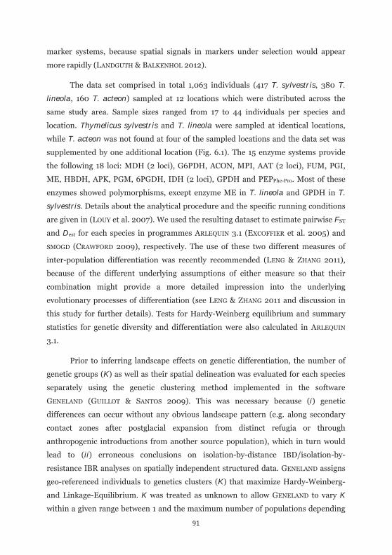
91
marker systems, because spatial signals in markers under selection would appear
more rapidly (LANDGUTH & BALKENHOL 2012).
The data set comprised in total 1,063 individuals (417 T. sylvestris, 380 T.
lineola, 160 T. acteon) sampled at 12 locations which were distributed across the
same study area. Sample sizes ranged from 17 to 44 individuals per species and
location. Thymelicus sylvestris and T. lineola were sampled at identical locations,
while T. acteon was not found at four of the sampled locations and the data set was
supplemented by one additional location (Fig. 6.1). The 15 enzyme systems provide
the following 18 loci: MDH (2 loci), G6PDH, ACON, MPI, AAT (2 loci), FUM, PGI,
ME, HBDH, APK, PGM, 6PGDH, IDH (2 loci), GPDH and PEPPhe-Pro. Most of these
enzymes showed polymorphisms, except enzyme ME in T. lineola and GPDH in T.
sylvestris. Details about the analytical procedure and the specific running conditions
are given in (LOUY et al. 2007). We used the resulting dataset to estimate pairwise FST
and Dest for each species in programmes ARLEQUIN 3.1 (EXCOFFIER et al. 2005) and
SMOGD (CRAWFORD 2009), respectively. The use of these two different measures of
inter-population differentiation was recently recommended (LENG & ZHANG 2011),
because of the different underlying assumptions of either measure so that their
combination might provide a more detailed impression into the underlying
evolutionary processes of differentiation (see LENG & ZHANG 2011 and discussion in
this study for further details). Tests for Hardy-Weinberg equilibrium and summary
statistics for genetic diversity and differentiation were also calculated in ARLEQUIN
3.1.
Prior to inferring landscape effects on genetic differentiation, the number of
genetic groups (K) as well as their spatial delineation was evaluated for each species
separately using the genetic clustering method implemented in the software
GENELAND (GUILLOT & SANTOS 2009). This was necessary because (i) genetic
differences can occur without any obvious landscape pattern (e.g. along secondary
contact zones after postglacial expansion from distinct refugia or through
anthropogenic introductions from another source population), which in turn would
lead to (ii) erroneous conclusions on isolation-by-distance IBD/isolation-by-
resistance IBR analyses on spatially independent structured data. GENELAND assigns
geo-referenced individuals to genetics clusters (K) that maximize Hardy-Weinberg-
and Linkage-Equilibrium. K was treated as unknown to allow GENELAND to vary K
within a given range between 1 and the maximum number of populations depending
92
on the species (i.e. 7 in T. acteon and 11 in both T. sylvestris and T. lineola). Markov
Chains were run for 3,000,000 generations and sampled every 1000th generation,
after an initial burn-in of 300 samples after thinning (10 %). Markov Chains with
these settings were run 10 times independently and the iteration with the highest log
posterior probability was chosen for inferring the most likely K and individual
assignments.
Figure 6.1: Locations of populations studied for all three Thymelicus species in southwestern Germany and adjoining areas in France and Luxemburg.
Modelling landscape effects on genetic differentiation
To test for landscape influences on genetic differentiation in each species, we
modeled multiple species distribution models (SDM) incorporating topographic,
bioclimatic and/or land use features. We then used resulting SDMs as resistance
surfaces to derive inter-population connectivity estimates based on electrical circuit
theory, and statistically compared these connectivity estimates to actual genetic
93
differentiation. SDMs are increasingly applied for resistance surface parameterization
in landscape genetic studies (POELCHAU & HAMRICK 2012, ORTEGO et al. 2012) even
under longer evolutionary time scales (BELL et al. 2009, DEVITT et al. 2013), since
they avoid the subjective parameterization of resistance surfaces which was criticized
in the past (SPEAR et al. 2010).
Species records
To model SDMs for the three Thymelicus species in the study area, presence data
were taken from personal observations of JCH, D. LOUY and T. SCHMITT (Germany)
covering the years 2003-2012. Further presence data were added from high
resolution records downloaded from the GBIF database (www.gbif.org). The final
datasets comprised 67 records for T. sylvestris, 62 for T. lineola and 28 records for T.
acteon. Given their specific habitat demands and the sampling effort that was
performed across the study area for either species (Fig. 6.1), we are confident to have
compiled a representative sample that covered the realized distribution of the species
in our study area.
Environmental layers
For construction of the SDMs, we used freely available GIS based environmental
layers. Bioclimatic data based on monthly averaged temperature and precipitation
data with 30 arc seconds spatial resolution was obtained from the Worldclim
Database (Vers. 1.4; www.worldclim.org; HIJMANS et al. 2005). The comprehensive
set of 19 bioclimatic variables are thought to be highly relevant for shaping species’
Grinnellian (abiotic) niches (BEAUMONT et al. 2005). In order to minimize the degree
of inter-correlation among the variables (i.e. to keep pair-wise Pearson´s R2< 0.75),
we selected a subset of variables (bio3, 7, 8, 9, 10, 11, 12, 15, 18, see Table 6.3 /
Appendix 6.S3 for definitions) which were assumed to be most relevant for the study
species. Topography-related data were derived from the SRTM Shuttle mission in 90
meters resolution (available through USGS seamless server; Table 6.S2). Based on
the altitude layers, we calculated slope and aspect using ARCGIS 9.3 (ESRI Redlands,
California, USA). Finally, CORINE land use related data was obtained from the
European Environmental Agency (www.eea.europa.eu). We either used CORINE
2006 data to assess current habitat availability as well as CORINE 1990 data for
94
assessing recent land use changes. All environmental layers were re-sampled to
uniform grid resolution of 90 m.
Calculating the Potential Connectivity Model
We defined a set of hypotheses based on the available environmental data and
generated five variable sets for comparing landscape effects on species-specific gene
flow (therein called scenarios, Table 6.S2). These scenarios represent various habitat
characteristics (i.e. climate, topography and land use) that were found to be
important for butterfly distributions at different spatial scales in previous studies
(WEISS et al. 1988; WARREN et al. 2001; PE’ER et al. 2004; 2006; PIN KOH 2007;
MARINI et al. 2009; FILZ et al. 2013a). Based on these variable sets and the respective
species records, we computed species distribution models (SDMs) with the software
MAXENT 3.3.3e (PHILLIPS et al. 2006) to generate maps displaying habitat suitability
for each species under a given scenario. As many other presence-pseudoabsence SDM
algorithms, MAXENT links environmental conditions at presence records of a given
taxon to those environmental conditions available within a specific geographic area
(background) to predict spatial patterns of environmental suitability. The SDM
output represents the likelihood of species potential occurrence across a geographic
area of interest (projection; for a detailed description see ELITH et al. 2011). We used
MAXENT instead of other available algorithms because it frequently outperforms other
approaches (ELITH et al. 2006; HEIKKINEN et al. 2006), even if the number of
presence locations is rather limited (HERNANDEZ et al. 2006; WISZ et al. 2008). We
ran MAXENT with the default settings but used a bootstrap approach, which allows
random selection of 70% of presence locations for model training and the remaining
30% for model testing. This procedure was repeated for 100 times and an averaged
map of suitable habitats was generated across all repetitions. As output we selected
the logistic format which ranges linearly from 0 (not suitable) to 1 (fully suitable). For
model evaluation, the area under the receiver operating characteristic curve (AUC)
was used (SWETS 1988). In particular, the AUC as internally computed in MAXENT is a
measure for the ability of the model to distinguish the given presence records from
the background data accounting for the proportion of the study area which is
predicted to be suitable for the target species (PHILLIPS et al. 2006). The AUC ranges
between 0.5 (random prediction) to 1.0 (perfect discrimination between presence and
pseudo-absence).
95
For the land use change scenario, we used land use data from CORINE 2006 as a
categorical environmental layer - just as we had done for the land use scenario.
However, we subsequently projected the model fit onto the CORINE 1990 layer to
assess habitat change in terms of a stability surface. The stability surface is the
average of both CORINE layers, with high values indicating suitable habitat patches
that remain stable over the 16 years time span, whereas low values represent low
habitat suitability, a strong habitat change in time, or both. This approach for
calculating stability surfaces is commonly used to estimate land use change and
habitat suitability across time (see BELL et al. 2006 and DEVITT et al. 2013 for
examples).
The resulting SDMs were used as conductance surfaces (i.e., high values indicate
good conductivity between two sites, whereas low values indicate poor conductivity;
MCRAE et al. 2008) in CIRCUITSCAPE v.3.4.1 to calculate resistances to movement and
gene flow among sampling locations (MCRAE et al. 2008). CIRCUITSCAPE is based on
electrical circuit theory, which was recently adapted from electrical engineering for
the assessment of landscape ecological questions (MCRAE et al. 2008). In particular,
CIRCUITSCAPE defines nodes (grid cells) and associated unit resistors (the resistance
value) that connecting two nodes and calculates resistance distances between focal
locations based on a nodal analysis algorithm as described in (MCRAE 2006). As the
habitat matrix had a very high extent (i.e. ~7.6 Mio. cells), we chose a four-neighbor-
connection scheme in order to meet the available computational capacities. It has
been previously shown that four and eight-neighbor-connection scheme lead to
highly similar outcomes (MCRAE & BEIER 2007).
Comparing connectivity estimates with genetic data
Resulting resistance values among locations were statistically compared to
estimates of genetic differentiation (i.e. FST and Dest) using linear regression models
as well as multiple regressions on distance matrices (MRDM; LICHSTEIN 2007) in R
v.2.14.1 (R DEVELOPMENT CORE TEAM 2012). For the linear regression models, the
Akaike Information Criterion corrected for small sample sizes (AICc) was used for
model comparisons within each species (BURNHAM & ANDERSON 2002). Despite their
sensitivity for non-independence in pair-wise comparisons, multi-model inference
based on information theory has been frequently applied in landscape genetic

96
analyses (GOLDBERG & WAITS 2010; RICHARDSON 2012) as the error entering the
comparison was assumed to be equal for each model, which did not affects model
ranking and thus still allows for assessing the relative model performance. To
ascertain results obtained with the AIC model selection, we also estimated
significance of MRDM models using 1,000 permutations. For MRDMs, the ecodist
package for R was used (GOSLEE & URBAN 2007).
Results
Genetic structures
No significant deviation from Hardy-Weinberg equilibrium was detected for any
population in the respective species. Genetic diversity was comparatively low in T.
lineola (mean ± SE; AR = 1.78 ± 0.17 HE = 9.6 ± 2.1, HO = 9.2 ± 2.1), while T. acteon
showed highest genetic diversities (AR = 1.88 ± 0.18, HE = 14.9 ± 2.9, HO = 12.5 ±
2.6). Thymelicus sylvestris showed an intermediate level of genetic diversity, as
compared to its congeners (AR = 1.80 ± 0.10, HE = 11.9 ± 1.5, HO = 11.0 ± 1.4). The
genetic differentiation was low in T. lineola (FST = 0.0081; Dest = 0.0012; p = n.s.),
while we detected highest genetic differentiation for T. acteon (FST = 0.0718; Dest =
0.0143; p < 0.0001). Again, Thymelicus sylvestris showed an intermediate level of
genetic differentiation, with a rather low among-population variance (FST = 0.0179;
Dest = 0.0039; p < 0.0001) (Table 6.1).
Table 6.1: Summary statistics for genetic diversity and differentiation for the three Tymelicusbuttlerflies.
T. lineola T. acteon T. sylvestris source
AR 1.78 ± 0.17 1.88 ± 0.18 1.80 ± 0.10 LOUY et al. 2007
HE 9.6 ± 2.1 14.9 ± 2.9 11.9 ± 1.5 LOUY et al. 2007
HO 9.2 ± 2.1 12.5 ± 2.6 11.0 ± 1.4 LOUY et al. 2007
Ptot 52.0 ± 9.7 66.0 ± 9.1 42.9 ± 7.9 LOUY et al. 2007
P95 36.4 ± 9.4 49.3 ± 13.4 32.3 ± 4.2 LOUY et al. 2007
FST 0.0081 0.0755 0.0179 LOUY et al. 2007
Dest 0.0012 0.0143 0.0039 HABEL et al. 2013
97
Genetic clustering results
The posterior density and log-likelihood levels of all GENELAND runs stabilized long
before the end of the Markov Chains, indicating that convergence was reached (Fig.
6.S1). For each of the species, all 10 replicate MCMC runs converged on K = 1
panmictic cluster (Fig. 6.S1), indicating no absolute barriers affecting IBD or IBR
assumptions.
Species Distribution Models
AUC values derived from the SDMs ranged from ‘poor’ (AUC = 0.66, scenarios
‘land use’ and ‘land use change’ in T. sylvestris, Table 6.2) to ‘good’ (AUC = 0.86,
scenario ‘all’ in T. lineola, Table 6.2) according to the classification scheme for model
quality from (ARAÚJO et al. 2005) adapted from (SWETS 1988). Variable contributions
in multi-factorial SDMs (scenarios ‘climate’, ‘topography’ and ‘all’) differed between
species (Table 6.3). For the topography scenario, slope contributed most to the SDM
in all three species, followed by aspect and altitude (Table 6.3). In T. acteon a
different set of variables had higher explanative power with respect to the climate
scenario. Here, precipitation of the warmest quarter (bio18) was most important,
followed by a set of temperature related variables (bio3, 7, 8, 9, 11; Table 6.3). In
contrast, Thymelicus lineola and T. sylvestris had very similar variable contributions
as a result of the highly similar distribution of occurrence records. In these species,
the mean temperature of the coldest quarter followed by the temperature annual
range contributed to more than half of the total model (Table 6.3). Finally,
considering the entire predictor set, a combination of slope and land use contributed
most in all species, but where T. lineola and T. sylvestris had again more similar
variable contributions rather than T. acteon (Table 6.3). In accordance, T. lineola and
T. sylvestris showed similar potential distributions containing large continuous areas
of high suitability, whereas T. acteon shows a highly patchy distribution with large
unsuitable areas surrounding potential habitat patches (Fig. 6.2).
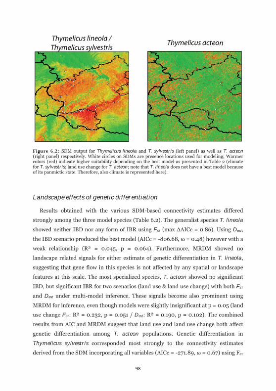
98
Figure 6.2: SDM output for Thymelicus lineola and T. sylvestris (left panel) as well as T. acteon (right panel) respectively. White circles on SDMs are presence locations used for modeling; Warmer colors (red) indicate higher suitability depending on the best model as presented in Table 2 (climate for T. sylvestris; land use change for T. acteon; note that T. lineola does not have a best model because of its panmictic state. Therefore, also climate is represented here).
Landscape effects of genetic differentiation
Results obtained with the various SDM-based connectivity estimates differed
strongly among the three model species (Table 6.2). The generalist species T. lineola
showed neither IBD nor any form of IBR using FST (max AICc = 0.86). Using Dest,
the IBD scenario produced the best model (AICc = -806.68, = 0.48) however with a
weak relationship (R² = 0.045, p = 0.064). Furthermore, MRDM showed no
landscape related signals for either estimate of genetic differentiation in T. lineola,
suggesting that gene flow in this species is not affected by any spatial or landscape
features at this scale. The most specialized species, T. acteon showed no significant
IBD, but significant IBR for two scenarios (land use & land use change) with both FST
and Dest under multi-model inference. These signals become also prominent using
MRDM for inference, even though models were slightly insignificant at p = 0.05 (land
use change FST: R² = 0.232, p = 0.051 / Dest: R² = 0.190, p = 0.102). The combined
results from AIC and MRDM suggest that land use and land use change both affect
genetic differentiation among T. acteon populations. Genetic differentiation in
Thymelicus sylvestris corresponded most strongly to the connectivity estimates
derived from the SDM incorporating all variables (AICc = -271.89, = 0.67) using FST
99
and the information-theoretic approach. The climate related scenario was also within
the most reliable models under AICc ( AICc = 1.65, = 0.29). However, MRDM
suggested that land use and land use change were also important for explaining
genetic differentiation in this species. The opposite becomes obvious using Dest as
differentiation metric. Here, the information theoretic approach reveals climate, land
use and land use change as highly informative, with climate being most important
(AIC = -723.08, = 0.45). Surprisingly, the scenario covering the entire variable set
contributed nearly no information ( AICc = 4.44, = 0.05). In addition, MRDM
highlighted only climate as significantly related to genetic differentiation. In
summary, the combined results of different differentiation metrics and inference
methods suggest that the climatic conditions across the study site deliver the most
important and stable relationship for adjusting gene flow in the intermediate species,
with additional effects of land use. Classical IBD received less support against IBR
models (Table 6.2, Fig. 6.S2) in all species. Interestingly, topography seems to play no
role at all for any of the species.
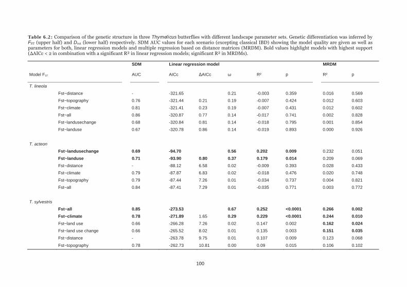
100
Table 6.2: Comparison of the genetic structure in three Thymelicus butterflies with different landscape parameter sets. Genetic differentiation was inferred by FST (upper half) and Dest (lower half) respectively. SDM AUC values for each scenario (excepting classical IBD) showing the model quality are given as well as parameters for both, linear regression models and multiple regression based on distance matrices (MRDM). Bold values highlight models with highest support ( AICc < 2 in combination with a significant R² in linear regression models; significant R² in MRDMs).
SDM Linear regression model MRDM
Model FST AUC AICc AICc R² p R² p
T. lineola Fst~distance - -321.65 0.21 -0.003 0.359 0.016 0.569
Fst~topography 0.76 -321.44 0.21 0.19 -0.007 0.424 0.012 0.603
Fst~climate 0.81 -321.41 0.23 0.19 -0.007 0.431 0.012 0.602
Fst~all 0.86 -320.87 0.77 0.14 -0.017 0.741 0.002 0.828
Fst~landusechange 0.68 -320.84 0.81 0.14 -0.018 0.795 0.001 0.854
Fst~landuse 0.67 -320.78 0.86 0.14 -0.019 0.893 0.000 0.926
T. acteon Fst~landusechange 0.69 -94.70 0.56 0.202 0.009 0.232 0.051
Fst~landuse 0.71 -93.90 0.80 0.37 0.179 0.014 0.209 0.069
Fst~distance - -88.12 6.58 0.02 -0.009 0.393 0.028 0.433
Fst~climate 0.79 -87.87 6.83 0.02 -0.018 0.476 0.020 0.748
Fst~topography 0.79 -87.44 7.26 0.01 -0.034 0.737 0.004 0.821
Fst~all 0.84 -87.41 7.29 0.01 -0.035 0.771 0.003 0.772
T. sylvestris Fst~all 0.85 -273.53 0.67 0.252 <0.0001 0.266 0.002 Fst~climate 0.78 -271.89 1.65 0.29 0.229 <0.0001 0.244 0.010 Fst~land use 0.66 -266.28 7.26 0.02 0.147 0.002 0.162 0.024 Fst~land use change 0.66 -265.52 8.02 0.01 0.135 0.003 0.151 0.035 Fst~distance - -263.78 9.75 0.01 0.107 0.009 0.123 0.068
Fst~topography 0.78 -262.73 10.81 0.00 0.09 0.015 0.106 0.102
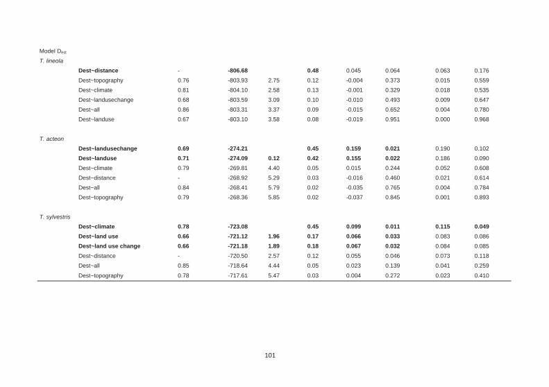
101
Model Dest T. lineola
Dest~distance - -806.68 0.48 0.045 0.064 0.063 0.176
Dest~topography 0.76 -803.93 2.75 0.12 -0.004 0.373 0.015 0.559
Dest~climate 0.81 -804.10 2.58 0.13 -0.001 0.329 0.018 0.535
Dest~landusechange 0.68 -803.59 3.09 0.10 -0.010 0.493 0.009 0.647
Dest~all 0.86 -803.31 3.37 0.09 -0.015 0.652 0.004 0.780
Dest~landuse 0.67 -803.10 3.58 0.08 -0.019 0.951 0.000 0.968
T. acteon Dest~landusechange 0.69 -274.21 0.45 0.159 0.021 0.190 0.102
Dest~landuse 0.71 -274.09 0.12 0.42 0.155 0.022 0.186 0.090
Dest~climate 0.79 -269.81 4.40 0.05 0.015 0.244 0.052 0.608
Dest~distance - -268.92 5.29 0.03 -0.016 0.460 0.021 0.614
Dest~all 0.84 -268.41 5.79 0.02 -0.035 0.765 0.004 0.784
Dest~topography 0.79 -268.36 5.85 0.02 -0.037 0.845 0.001 0.893
T. sylvestris Dest~climate 0.78 -723.08 0.45 0.099 0.011 0.115 0.049 Dest~land use 0.66 -721.12 1.96 0.17 0.066 0.033 0.083 0.086
Dest~land use change 0.66 -721.18 1.89 0.18 0.067 0.032 0.084 0.085
Dest~distance - -720.50 2.57 0.12 0.055 0.046 0.073 0.118
Dest~all 0.85 -718.64 4.44 0.05 0.023 0.139 0.041 0.259
Dest~topography 0.78 -717.61 5.47 0.03 0.004 0.272 0.023 0.410
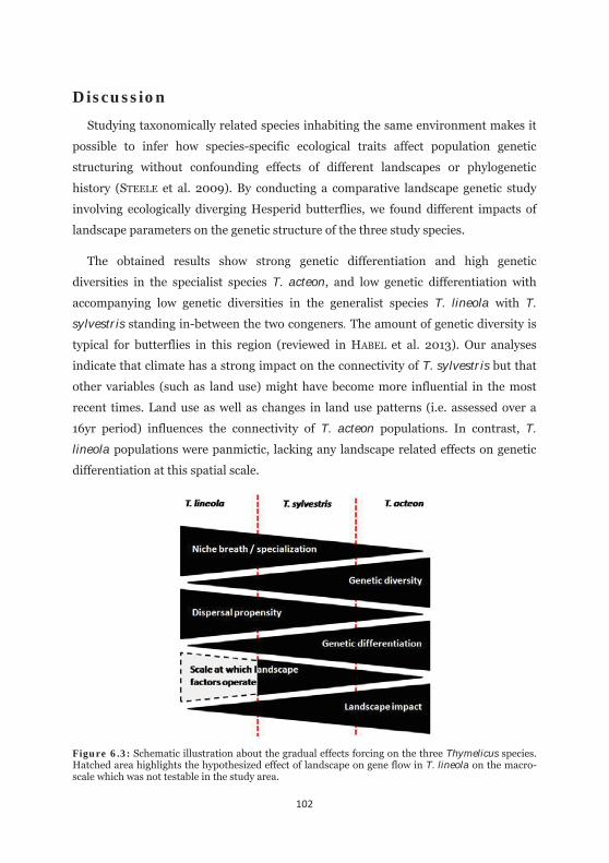
102
Discussion
Studying taxonomically related species inhabiting the same environment makes it
possible to infer how species-specific ecological traits affect population genetic
structuring without confounding effects of different landscapes or phylogenetic
history (STEELE et al. 2009). By conducting a comparative landscape genetic study
involving ecologically diverging Hesperid butterflies, we found different impacts of
landscape parameters on the genetic structure of the three study species.
The obtained results show strong genetic differentiation and high genetic
diversities in the specialist species T. acteon, and low genetic differentiation with
accompanying low genetic diversities in the generalist species T. lineola with T.
sylvestris standing in-between the two congeners. The amount of genetic diversity is
typical for butterflies in this region (reviewed in HABEL et al. 2013). Our analyses
indicate that climate has a strong impact on the connectivity of T. sylvestris but that
other variables (such as land use) might have become more influential in the most
recent times. Land use as well as changes in land use patterns (i.e. assessed over a
16yr period) influences the connectivity of T. acteon populations. In contrast, T.
lineola populations were panmictic, lacking any landscape related effects on genetic
differentiation at this spatial scale.
Figure 6.3: Schematic illustration about the gradual effects forcing on the three Thymelicus species. Hatched area highlights the hypothesized effect of landscape on gene flow in T. lineola on the macro-scale which was not testable in the study area.
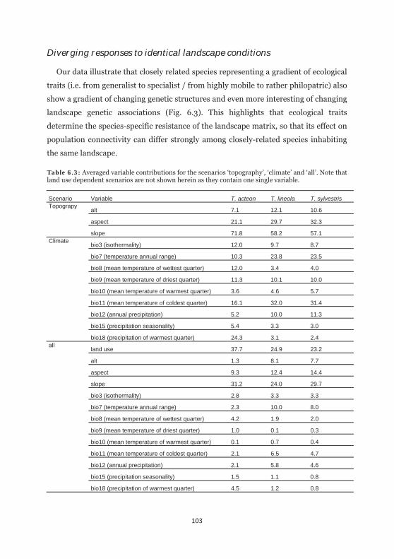
103
Diverging responses to identical landscape conditions
Our data illustrate that closely related species representing a gradient of ecological
traits (i.e. from generalist to specialist / from highly mobile to rather philopatric) also
show a gradient of changing genetic structures and even more interesting of changing
landscape genetic associations (Fig. 6.3). This highlights that ecological traits
determine the species-specific resistance of the landscape matrix, so that its effect on
population connectivity can differ strongly among closely-related species inhabiting
the same landscape.
Table 6.3: Averaged variable contributions for the scenarios ‘topography’, ‘climate’ and ‘all’. Note that land use dependent scenarios are not shown herein as they contain one single variable.
Scenario Variable T. acteon T. lineola T. sylvestris Topograpy
alt 7.1 12.1 10.6
aspect 21.1 29.7 32.3
slope 71.8 58.2 57.1 Climate
bio3 (isothermality) 12.0 9.7 8.7
bio7 (temperature annual range) 10.3 23.8 23.5
bio8 (mean temperature of wettest quarter) 12.0 3.4 4.0
bio9 (mean temperature of driest quarter) 11.3 10.1 10.0
bio10 (mean temperature of warmest quarter) 3.6 4.6 5.7
bio11 (mean temperature of coldest quarter) 16.1 32.0 31.4
bio12 (annual precipitation) 5.2 10.0 11.3
bio15 (precipitation seasonality) 5.4 3.3 3.0
bio18 (precipitation of warmest quarter) 24.3 3.1 2.4 all
land use 37.7 24.9 23.2
alt 1.3 8.1 7.7
aspect 9.3 12.4 14.4
slope 31.2 24.0 29.7
bio3 (isothermality) 2.8 3.3 3.3
bio7 (temperature annual range) 2.3 10.0 8.0
bio8 (mean temperature of wettest quarter) 4.2 1.9 2.0
bio9 (mean temperature of driest quarter) 1.0 0.1 0.3
bio10 (mean temperature of warmest quarter) 0.1 0.7 0.4
bio11 (mean temperature of coldest quarter) 2.1 6.5 4.7
bio12 (annual precipitation) 2.1 5.8 4.6
bio15 (precipitation seasonality) 1.5 1.1 0.8
bio18 (precipitation of warmest quarter) 4.5 1.2 0.8
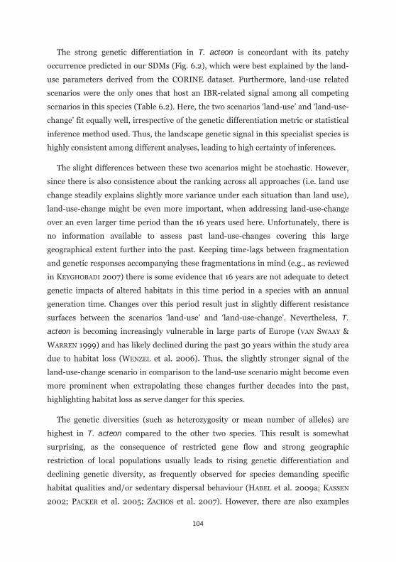
104
The strong genetic differentiation in T. acteon is concordant with its patchy
occurrence predicted in our SDMs (Fig. 6.2), which were best explained by the land-
use parameters derived from the CORINE dataset. Furthermore, land-use related
scenarios were the only ones that host an IBR-related signal among all competing
scenarios in this species (Table 6.2). Here, the two scenarios ‘land-use’ and ‘land-use-
change’ fit equally well, irrespective of the genetic differentiation metric or statistical
inference method used. Thus, the landscape genetic signal in this specialist species is
highly consistent among different analyses, leading to high certainty of inferences.
The slight differences between these two scenarios might be stochastic. However,
since there is also consistence about the ranking across all approaches (i.e. land use
change steadily explains slightly more variance under each situation than land use),
land-use-change might be even more important, when addressing land-use-change
over an even larger time period than the 16 years used here. Unfortunately, there is
no information available to assess past land-use-changes covering this large
geographical extent further into the past. Keeping time-lags between fragmentation
and genetic responses accompanying these fragmentations in mind (e.g., as reviewed
in KEYGHOBADI 2007) there is some evidence that 16 years are not adequate to detect
genetic impacts of altered habitats in this time period in a species with an annual
generation time. Changes over this period result just in slightly different resistance
surfaces between the scenarios ‘land-use’ and ‘land-use-change’. Nevertheless, T.
acteon is becoming increasingly vulnerable in large parts of Europe (VAN SWAAY &
WARREN 1999) and has likely declined during the past 30 years within the study area
due to habitat loss (WENZEL et al. 2006). Thus, the slightly stronger signal of the
land-use-change scenario in comparison to the land-use scenario might become even
more prominent when extrapolating these changes further decades into the past,
highlighting habitat loss as serve danger for this species.
The genetic diversities (such as heterozygosity or mean number of alleles) are
highest in T. acteon compared to the other two species. This result is somewhat
surprising, as the consequence of restricted gene flow and strong geographic
restriction of local populations usually leads to rising genetic differentiation and
declining genetic diversity, as frequently observed for species demanding specific
habitat qualities and/or sedentary dispersal behaviour (HABEL et al. 2009a; KASSEN
2002; PACKER et al. 2005; ZACHOS et al. 2007). However, there are also examples
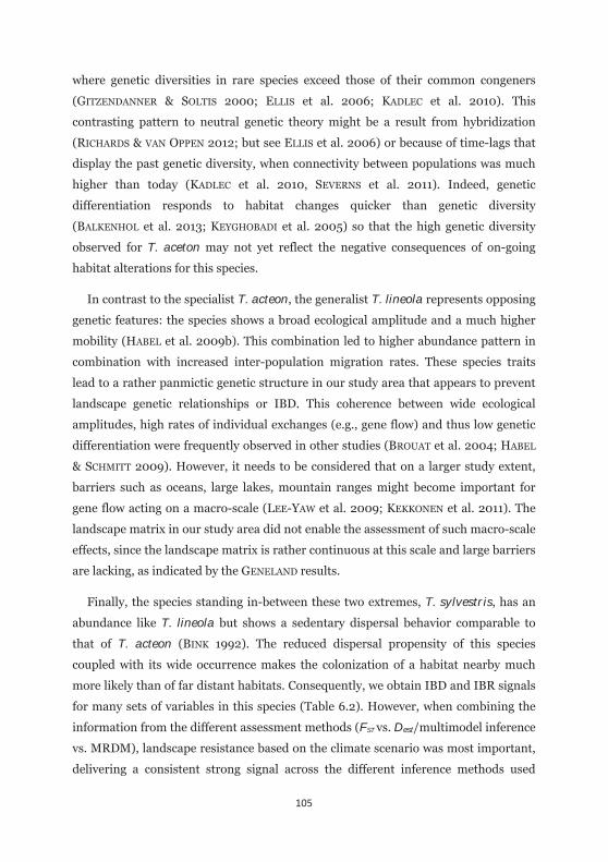
105
where genetic diversities in rare species exceed those of their common congeners
(GITZENDANNER & SOLTIS 2000; ELLIS et al. 2006; KADLEC et al. 2010). This
contrasting pattern to neutral genetic theory might be a result from hybridization
(RICHARDS & VAN OPPEN 2012; but see ELLIS et al. 2006) or because of time-lags that
display the past genetic diversity, when connectivity between populations was much
higher than today (KADLEC et al. 2010, SEVERNS et al. 2011). Indeed, genetic
differentiation responds to habitat changes quicker than genetic diversity
(BALKENHOL et al. 2013; KEYGHOBADI et al. 2005) so that the high genetic diversity
observed for T. aceton may not yet reflect the negative consequences of on-going
habitat alterations for this species.
In contrast to the specialist T. acteon, the generalist T. lineola represents opposing
genetic features: the species shows a broad ecological amplitude and a much higher
mobility (HABEL et al. 2009b). This combination led to higher abundance pattern in
combination with increased inter-population migration rates. These species traits
lead to a rather panmictic genetic structure in our study area that appears to prevent
landscape genetic relationships or IBD. This coherence between wide ecological
amplitudes, high rates of individual exchanges (e.g., gene flow) and thus low genetic
differentiation were frequently observed in other studies (BROUAT et al. 2004; HABEL
& SCHMITT 2009). However, it needs to be considered that on a larger study extent,
barriers such as oceans, large lakes, mountain ranges might become important for
gene flow acting on a macro-scale (LEE-YAW et al. 2009; KEKKONEN et al. 2011). The
landscape matrix in our study area did not enable the assessment of such macro-scale
effects, since the landscape matrix is rather continuous at this scale and large barriers
are lacking, as indicated by the GENELAND results.
Finally, the species standing in-between these two extremes, T. sylvestris, has an
abundance like T. lineola but shows a sedentary dispersal behavior comparable to
that of T. acteon (BINK 1992). The reduced dispersal propensity of this species
coupled with its wide occurrence makes the colonization of a habitat nearby much
more likely than of far distant habitats. Consequently, we obtain IBD and IBR signals
for many sets of variables in this species (Table 6.2). However, when combining the
information from the different assessment methods (FST vs. Dest/multimodel inference
vs. MRDM), landscape resistance based on the climate scenario was most important,
delivering a consistent strong signal across the different inference methods used
106
(Table 6.2, see also below). This contrasts to the IBR of T. acteon, where climate plays
no role at all. In contrast to land-use, climate acts on a meso-scale at our study area
(i.e., masking larger areas of the study extent rather than small habitat patches). In T.
sylvestris the climate related SDM revealed high resistances along river valleys as
well as on the higher elevations of the low mountain ranges (Fig. 6.2). These potential
barriers act at a much larger scale and extent compared to the small and patchy
habitat islands enclosed by more or less unfavourable habitats in T. acteon.
Consequently, the different landscape features contributing to the IBR signals in
these two species highlight the importance of scale and shape of the connective
elements (or their respective barriers) in the landscape matrix where methodological
shortcomings can be excluded (ENGLER, unpublished). However, the obtained IBR
models explain only up to 24 % of the variance in our dataset. That in turn indicates
that the remaining variance of our data can only be explained by additional factors
such as ecological traits and habitat requirements. These can be even more relevant
for butterfly species than habitat size and habitat isolation, e.g. as shown for the
Heath butterfly Coenonympha tullia (DENNIS & EALES 1997). Nevertheless, the extent
of the relationships in our IBD/IBR comparisons are in concert with other studies
(GROOT et al. 2011) indicating that gene flow can be interpreted as an important
component out of a variety of mechanisms influencing population genetic structure.
Accounting for FST and Dest in landscape genetic studies
Interestingly, in the case of Thymelicus sylvestris, the prominent signal under FST
arising from the SDM using all landscape variables becomes completely eliminated
when using Dest as a differentiation metric. The fact that different metrics can lead to
different conclusions is also evident in the ongoing debate about the utility of
different genetic differentiation measures (HELLER & SIEGISMUND 2009; RYMAN &
LEIMAR 2009; JOST 2009; GERLACH et al. 2010; MEIRMANS & HEDRICK 2011;
RAEYMAEKERS et al. 2012). For example, traditional FST-like metrics are more sensitive
to recent demographic changes (which depends e.g. on effective population size) than
metrics which are independent of effective population size, such as Dest (LENG &
ZHANG 2011; RYMAN & LEIMAR 2009; MEIRMANS & HEDRICK 2011; RAEYMAEKERS et al.
2012). This makes FST more sensible to effects of gene flow or drift in comparison to
Dest. Thus, from a landscape genetic perspective, using different types of
107
differentiation metrics allows to test for the contribution of landscape effects in
contemporary versus past times. If landscape composition change over time (and
consequently the amount of gene flow mediated by the landscape), FST would respond
much quicker to those changes while Dest remains rather stable over time. In the case
of Thymelicus sylvestris, this means that Dest may highlight the landscape effect (here
climate) of highest importance for gene flow in this species in former times, whereas
FST highlights more recent landscape effects on genetic structure that involves also
other landscape elements beside climate such as land use and topographical
elements.
In contrast to the climate-only scenario, connectivity estimates involving all
variables did not give highest importance to climatic factors. In particular, land use
and slope contribute almost 54% of the total importance of this scenario, whereas the
best performing variables from the climate scenario, bio11 (mean temp of coldest
quarter) and bio7 (temp annual range) that contribute together 54.9%, contributing
under the full model just 12.7% of the total importance. This might highlight the
change of landscape factors important to gene flow in this species. As T. sylvestris is
indeed common but not very mobile, anthropogenic land transformations of the past
decades might now lead to a stronger fragmentation of populations which ultimately
lead to changes in the contributions of landscape factors shaping gene flow as shown
elsewhere (PAVLACKY et al. 2009). Consequently, this might mean that this species is
just at the tipping point of being of conservation concern (sensu HABEL & SCHMITT
2012) where population trends swapping from stable to decreasing. Its congeners T.
acteon and T. lineola showing both consistent results across the different metrics
underpinning their stable state in terms of their abundance (insentinent and
widespread vs. sensible and endangered) and specialization (generalist vs. specialist).
Conclusion
Taxonomically close relatives serve as ideal model systems to study interspecific
characteristics in ecological traits without confounding effects derived from different
evolutionary histories. Yet, studies investigating the role of landscape on gene flow of
closely related taxa inhabiting the same environment are still scarce. Our results
reveal that even between sibling species, gene flow is affected by the landscape in very
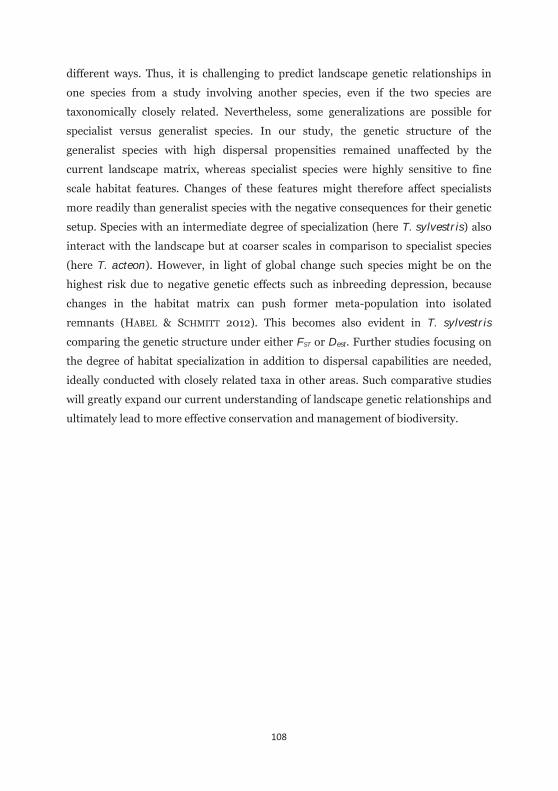
108
different ways. Thus, it is challenging to predict landscape genetic relationships in
one species from a study involving another species, even if the two species are
taxonomically closely related. Nevertheless, some generalizations are possible for
specialist versus generalist species. In our study, the genetic structure of the
generalist species with high dispersal propensities remained unaffected by the
current landscape matrix, whereas specialist species were highly sensitive to fine
scale habitat features. Changes of these features might therefore affect specialists
more readily than generalist species with the negative consequences for their genetic
setup. Species with an intermediate degree of specialization (here T. sylvestris) also
interact with the landscape but at coarser scales in comparison to specialist species
(here T. acteon). However, in light of global change such species might be on the
highest risk due to negative genetic effects such as inbreeding depression, because
changes in the habitat matrix can push former meta-population into isolated
remnants (HABEL & SCHMITT 2012). This becomes also evident in T. sylvestris
comparing the genetic structure under either FST or Dest. Further studies focusing on
the degree of habitat specialization in addition to dispersal capabilities are needed,
ideally conducted with closely related taxa in other areas. Such comparative studies
will greatly expand our current understanding of landscape genetic relationships and
ultimately lead to more effective conservation and management of biodiversity.

109
Supplementary material
Table 6.S1: Geographic coordinates of the sampling locations. ID numbers correspond to those stated in Fig. 6.1.
Location – ID lat lon T. sylvestris T. lineola T. acteon
Niedergailbach – 1 49.128 7.220 x x x
Mimbach/Badstube - 2 49.212 7.296 x x
Montenach - 3 49.425 6.388 x
Eiderberg/Freudenburg - 4 49.549 6.537 x x
Niederanven - 5 49.664 6.252 x x x
Wasserliesch - 6 49.696 6.527 x x x
Echternacherbrück - 7 49.819 6.428 x x x
Ourtal - 8 49.882 6.275 x x x
Römersköpfchen - 9 49.921 6.446 x x x
Bettingen - 10 49.942 6.427 x x x
Schönecken - 11 50.144 6.462 x x
Weinsheim/Prüm - 12 50.224 6.488 x x
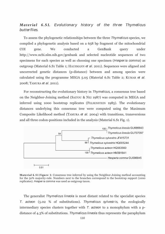
110
Material 6.S1. Evolutionary history of the three Thymelicus butterflies.
To assess the phylogenetic relationships between the three Thymelicus species, we
compiled a phylogenetic analysis based on a 658 bp fragment of the mitochondrial
COI gene. We conducted a GenBank query under
http://www.ncbi.nlm.nih.gov/genbank and selected nucleotide sequences of two
specimens for each species as well as choosing one specimen (Hesperia comma) as
outgroup (Material 6.S1 Table 1; HAUSMANN et al. 2011). Sequences were aligned and
uncorrected genetic distances (p-distance) between and among species were
calculated using the programme MEGA 5.05 (Material 6.S1 Table 2; KUMAR et al.
2008; TAMURA et al. 2011).
For reconstructing the evolutionary history in Thymelicus, a consensus tree based
on the Neighbor-Joining method (SAITOU & NEI 1987) was computed in MEGA and
inferred using 1000 bootstrap replicates (FELSENSTEIN 1985). The evolutionary
distances underlying this consensus tree were computed using the Maximum
Composite Likelihood method (TAMURA et al. 2004) with transitions, transversions
and all three codon-positions included in the analysis (Material 6.S1 Fig. 1).
Material 6.S1 Figure 1: Consensus tree inferred by using the Neighbor-Joining method accounting for the 50% majority-rule. Numbers next to the branches correspond to the bootstrap support (1000 replicates). Hesperia comma was used as outgroup taxon.
The generalist Thymelicus lineola is most distant related to the specialist species
T. acteon (5.02 % of substitutions). Thymelicus sylvestris, the ecologically
intermediary species clusters together with T. acteon to a monophylum with a p-
distance of 4.3% of substitutions. Thymelicus lineola thus represents the paraphylum
111
to the other two species because of a slightly higher genetic distance to T. sylvestris
(4.5%).
Material 6.S1 Table 1: Species and GenBank accession numbers of the individuals used for estimating genetic distance between species.
Species GenBank accession no.
Thymelicus lineola GU686843 Thymelicus lineola GU707097 Thymelicus sylvestris JF415731 Thymelicus sylvestris HQ005244 Thymelicus acteon HQ563560 Thymelicus acteon HM391841
Hesperia comma GU096945
Material 6.S1 Table 2: Uncorrected pairwise genetic distance (average %) of the COI sequences within (diagonal) and between (below diagonal) species of the genus Thymelicus.
T. acteon T. lineola T. sylvestris
Thymelicus acteon (n = 2) 0.00
Thymelicus lineola (n = 2) 5.02 0.00
Thymelicus sylvestris (n = 2) 4.30 4.50 0.15
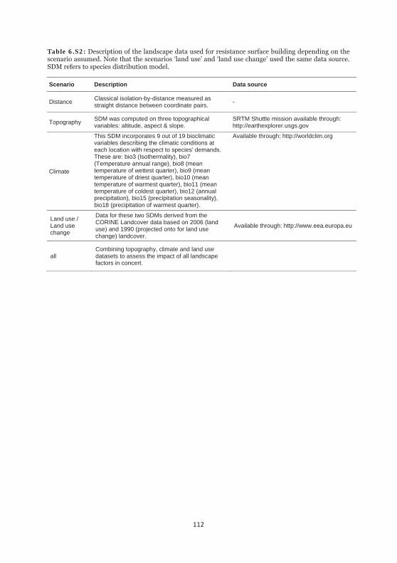
112
Table 6.S2: Description of the landscape data used for resistance surface building depending on the scenario assumed. Note that the scenarios ‘land use’ and ‘land use change’ used the same data source. SDM refers to species distribution model.
Scenario Description Data source
Distance Classical isolation-by-distance measured as straight distance between coordinate pairs. -
Topography SDM was computed on three topographical variables: altitude, aspect & slope.
SRTM Shuttle mission available through: http://earthexplorer.usgs.gov
Climate
This SDM incorporates 9 out of 19 bioclimatic variables describing the climatic conditions at each location with respect to species' demands. These are: bio3 (Isothermality), bio7 (Temperature annual range), bio8 (mean temperature of wettest quarter), bio9 (mean temperature of driest quarter), bio10 (mean temperature of warmest quarter), bio11 (mean temperature of coldest quarter), bio12 (annual precipitation), bio15 (precipitation seasonality), bio18 (precipitation of warmest quarter).
Available through: http://worldclim.org
Land use / Land use change
Data for these two SDMs derived from the CORINE Landcover data based on 2006 (land use) and 1990 (projected onto for land use change) landcover.
Available through: http://www.eea.europa.eu
all Combining topography, climate and land use datasets to assess the impact of all landscape factors in concert.
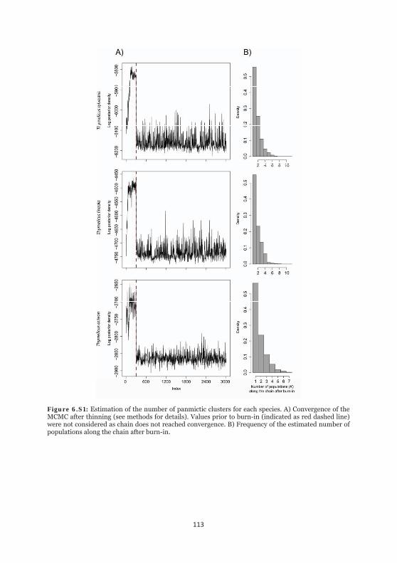
113
Figure 6.S1: Estimation of the number of panmictic clusters for each species. A) Convergence of the MCMC after thinning (see methods for details). Values prior to burn-in (indicated as red dashed line) were not considered as chain does not reached convergence. B) Frequency of the estimated number of populations along the chain after burn-in.
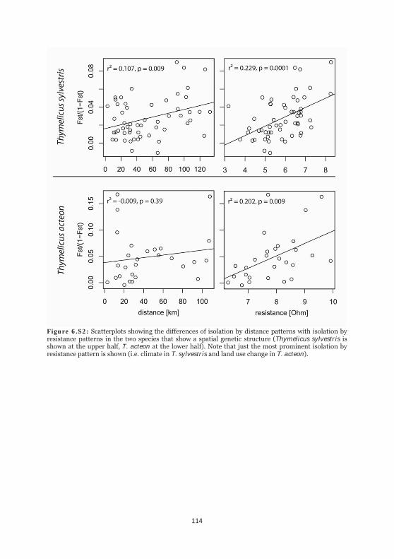
114
Figure 6.S2: Scatterplots showing the differences of isolation by distance patterns with isolation by resistance patterns in the two species that show a spatial genetic structure (Thymelicus sylvestris is shown at the upper half, T. acteon at the lower half). Note that just the most prominent isolation by resistance pattern is shown (i.e. climate in T. sylvestris and land use change in T. acteon).

115

116

117
CHAPTER 7
A statistical learning approach to improve ecological
inferences in landscape genetics by accounting for spatial
nonstationarity of genetic differentiation
“In a variable world, averages mostly are just meaningless, unimportant epiphenomena.”
JEREMY FOX

118
The work was conducted in collaboration with NIKO BALKENHOL.
119
Introduction
Landscapes are by definition heterogeneous in space (WU 2012), so that certain
landscape elements can be driving ecological processes in some areas while being
irrelevant in others. Gene flow is one of these processes, and a central goal of the
emerging field of landscape genetics is to understand how and why gene flow is
affected by the landscape (MANEL et al. 2003; MANEL & HOLDEREGGER 2013).
Therefore, many studies in this field correlate gene flow estimates between sampled
locations (i.e., genetic distances) with effective distances, as inferred from the
surrounding landscape matrix. Usually, this relationship is unknown, which is why
researchers compare genetic distances against a set of different landscape variables to
find the strongest correlation (Fig. 7.1). This quantifies the strongest average
landscape effect within the study area, yet it largely ignores the heterogeneous and
dynamic nature of the landscape itself. In consequence, this approach often leads to a
high amount of unexplained variance in gene flow – landscape relationships, which
could be caused, in part, by spatial nonstationarity in gene flow patterns (DUFORET-
FREBOURG & BLUM 2014).
Spatial nonstationarity refers to the inconsistent relationships of one or many
predictor variables to a response variable across space (BRUNSDON et al. 1996). In our
case, if gene flow is affected by spatial nonstationarity, it is because migration rates
vary across a given study area. For instance, this variation could be masked by
demographic discontinuities at local populations across a species’ range, or due to
landscape effects that directly affect migration rates. In the latter case, exploratory
analyses could link different landscape elements to measures of gene flow to test for
spatial nonstationarity. One way of doing this is to focus on sampling designs that
separate the study area into homogenous parts and restrict comparisons only within
these local subsets. However, this strategy has two major drawbacks: first, it would
decrease the power of analysis, as comparisons located between these local subsets
will consequently get lost; second, most landscapes are complex mosaics of
continuously changing elements affected by many interactions in time and space
(e.g., disturbance dynamics; TURNER 2010). Therefore, a spatial segregation is hard to
realize and is largely impractical—especially when the study extent and/or spatial
scale of interest is large.
120
Here, we propose an alternative approach to assess spatial nonstationarity which is
based on statistical learning theory. This theory considers learning as the challenge
of finding the most appropriate function (f) from empirical data (VAPNIK 2013). In
landscape genetics, this learning is mostly supervised, as for each response
measurement (i.e., the genetic distance) there are one or more associated predictor
measurements available (i.e., the effective distances of different landscape elements).
In a simplified way, this relationship can be expressed as:
Y = f(X) + ,
where the genetic distance is the response variable Y, to one or several predictor
variables X, such as effective environmental distances, which are framed in a function
f, and supplemented by a random error term .
In this general relationship, where Y and X are known, two sources of error exist:
the reducible error and the irreducible error. The reducible error is linked to the
unknown function f, which represents the systematic information that X provides
about Y (JAMES et al. 2013). It can be reduced by learning, which is the most
appropriate statistical method to estimate f (JAMES et al. 2013). In landscape genetics,
a plethora of statistical methods exist to estimate f, even though there is an ongoing
debate about which methods are the most appropriate (e.g., BALKENHOL et al. 2009;
JAQUIÉRY et al. 2011; DYER 2015a). The irreducible error is the amount of error that
remains after improving f, hence it characterizes variance in Y that cannot be
explained by X using f, and is expressed by the random error term . This source of
error has thus far received little attention in landscape genetics, focusing on limits of
measurements of X or Y (e.g., SPEAR 2010; DYER 2015a) but not on the dynamic
nature of the landscape itself that could be the cause of spatial nonstationarity
patterns in migration rates (DUFORET-FREBOURG & BLUM 2014).
Here, we argue that a large fraction of the irreducible error is systemic, because
the way landscape patterns are characterized to correlate X with Y across a study area
typically ignores the spatial heterogeneity and temporal dynamics of the landscape.
To account for this systemic error, we present a framework that improves f by
assembling a single solution for X under any situation where nX > 1. This is achieved
by choosing the landscape element Xj for a single comparison j with Yj out of a
number of n available landscape elements Xj1, Xj2, … Xjn that minimize the irreducible

121
error (Fig. 7.2). In other words, using the information about genetic exchange, we
compile a new predictor variable called, landscape, from a number of existing
predictors covering different but complementary information (such as climate,
topography, or landuse) to address spatial nonstationarity . Each single predictor
does not account for possible limits of genetic measurements at single comparisons
that could be driven by one of the remaining predictors. This can lead to higher
amounts of unexplained variance (Fig. 7.1). We exemplify this framework with two
empirical datasets of (1) a Central European Hesperid butterfly (LOUY et al. 2007;
ENGLER et al. 2014), as well as (2) the wolverine (Gulo gulo) across its Nearctic range
(KYLE & STROBECK 2001; MCRAE & BEIER 2007). We discuss the results and its
implications for study design and inference in landscape genetics.
Figure 7.1: A fictive study area that comprises seven localities where genetic information from a species was obtained but where relationships to landscape elements are unknown (left). The goal is to relate the estimated genetic distance (distgen) to a set of effective distances (disteff) estimated for each of three landscape elements (yellow, red, and blue). The amount of explained variance increases from the yellow to the blue landscape element (right). All comparisons still lead to a high amount of unexplained variance.
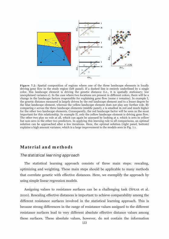
122
Figure 7.2: Spatial composition of regions where one of the three landscape elements is locally driving gene flow in the study region (left panel). If a dashed line is entirely underlined by a single color, this landscape element is driving the genetic distance (i.e., it is spatially stationary; low unexplained variance ). In the case where two locations are present in different colors, there will be a change in the landscape factors responsible for explaining gene flow (some remains). In example I, the genetic distance measured is largely driven by the red landscape element and to a lesser degree by the blue landscape element, whereas the yellow landscape element does not play any further role. By comparing across the three landscape elements (middle panel), is smallest in red and much higher for the other two landscape elements. Consequently, the red landscape factor will be seen as the most important for this relationship. In example II, only the yellow landscape element is driving gene flow. The other two play no role at all, which can again be assessed by looking at , which is zero in yellow but non-zero in the other two predictors. In applying this learning rule to all comparisons, an optimal solution can be approached after a few iterations. Here, the optimal solution (right panel, bottom) explains a high amount variance, which is a large improvement to the models seen in Fig. 7.1.
Material and methods
The statistical learning approach
The statistical learning approach consists of three main steps: rescaling,
optimizing and weighting. These main steps should be applicable to many methods
that correlate genetic with effective distances. Here, we exemplify the approach by
using simple linear regression models.
Assigning values to resistance surfaces can be a challenging task (SPEAR et al.
2010). Rescaling effective distances is important to achieve comparability among the
different resistance surfaces involved in the statistical learning approach. This is
because strong differences in the range of resistance values assigned to the different
resistance surfaces lead to very different absolute effective distance values among
these surfaces. These absolute values, however, do not contain the information
123
needed; it is their relative distance to each other that relates to the genetic distance.
In rescaling absolute values to percentiles, the important information is kept and
becomes comparable to effective distances from other resistance surfaces.
The percentiles of the effective distances (i.e. predictors X1 to Xn) are initially
compared against a reference model of isolation-by-distance (IBD) based on
percentiles of geographical distance values. From this model, residuals are predicted
for each of the predictors. The effective distance with the smallest residual for each
comparison can now be selected to calculate a new comparison with the genetic
distance. Using linear regressions in our example, this will lead to a reduction of the
mean squared error (MSE), hence resulting in a higher r². From that model, the
residuals for each predictor will be updated and the selection continues for a novel
iteration. This process is repeated until r² remains constant (i.e., is minimized). The
optimization procedure returns a vector of the predictor most responsible for each
case, as well as a vector of the residual difference to the next closest residual. The
latter information can then be used to weight each case in the optimized solution.
We assume that weighting can improve the effect size of driving landscape
elements to functional connectivity and thereby the relationship between genetic and
effective distances. Comparisons, where a single predictor best explains the genetic
distance, show a high difference in residual distances of this predictor to other
predictors. In turn, if residual distances are very equal to each other, one predictor
could be replaced by another one without having a strong effect on the entire
relationship. The weighting itself is also an optimizing process, as there could be
instances where weighting does not add to overall model improvement.
These three steps have been compiled in r-code using the RASTER, SCALES and
VEGAN packages in R 3.0.2 (WICKHAM 2012; R CORE TEAM 2013; HIJMANS & VAN
ETTEN 2012; OKSANEN et al. 2014), and can be found in the supplementary material
together with code for plotting using the SP package (BIVAND et al. 2013).
Empirical examples
To test the performance of this statistical approach, we used two empirical
examples from the literature. Both examples have known relationships between
124
genetic and effective distances, but differ in the study extent and the number of
landscape variables.
The first example covers the local distribution of the Hesperid butterfly
Thymelicus sylvestris in Southwest Germany and adjacent areas in Luxemburg and
France (LOUY et al. 2007, ENGLER et al. 2014). It has been shown that the species’
genetic differentiation is characterized IBD (LOUY et al. 2007) and even stronger
signals of isolation-by-resistance (IBR) of different landscape elements could be
found recently (ENGLER et al. 2014). Herein, climate has been identified as the
landscape element with the highest information content for explaining gene flow of
this species in this region (ENGLER et al. 2014). The landscape across the study area is
characterized by a mosaic of different land uses as well as a topographic relief,
including distinct mountain ridges and two major river valleys, which also affects
local climate. The effective distances used for this study were calculated among
eleven sample sites with available genetic information by using three resistance
surfaces characterizing climatic, topographic, and land-use information. Calculations
were performed in CIRCUITSCAPE (v 3.4.1; MCRAE et al. 2008), and resistance surfaces
were parameterized using species distribution models (SDM; see ENGLER et al. 2014
for details).
The second example focuses on the Nearctic distribution of the wolverine (Gulo
gulo). Across that range, twelve populations were genetically characterized (KYLE &
STROBECK 2001) and later tested for IBR patterns based on the species’ range shape
(MCRAE & BEIER 2007). For our study, we used the species’ pairwise genetic
differentiation estimates (FST) from KYLE & STROBECK (2001), range shape
information from WILSON (1982), and generated an SDM based on climate condition
and occurrence information across continental North America (Supplementary
Information). The wolverine strongly depends on the retainment of snow in spring
(MAGOUN & COPELAND 1998; AUBRY et al. 2007; COPELAND et al. 2010), which makes
climate an inherent factor of its distribution. We calculated effective distances in the
pairwise mode of CIRCUITSCAPE by using a focal points table within an eight-neighbor-
connection scheme among the genetically sampled sites for the resistance surfaces
‘range’ and ‘climate’.
125
Results
Both empirical examples increase the amount of explained variance after applying
the statistical learning approach, thereby reducing the MSE and thus the irreducible
error . The r² increased in T. sylvestris from 0.107 under IBD to 0.574 for the
optimized solution after only four iterations. In the wolverine example, the approach
also took only four iterations to increase the r² from 0.292 under IBD to 0.771 in the
optimized solution. The weighted solution further increased the r² values to 0.599 in
T. sylvestris and to 0.774 in the wolverine, respectively.
All of the three assessed landscape elements in T. sylvestris showed significant
IBR (ENGLER et al. 2014), yet r² values varied from 0.09 in topography, to over 0.147
in land use, and 0.229 when taking climatic conditions into account (Fig. 7.3). The
weighted and optimized solution shows a high admixture of the three landscape
elements involved in the compilation with genetic distances. Here, 23 out of 55
comparisons were assigned to climate, 17 to topography, and 15 to land use. The
highest weights (i.e., comparisons where one landscape element outcompetes
another) were found in climate, while weights were generally weaker for the other
landscape elements (Fig. 7.3). Plotting this information as a network in the study area
confirms the strong interplay of the different landscape elements as driving factors
for gene flow, but also highlights two sites with a clustering of comparisons with high
weights (Fig. 7.4).
In the wolverine example, the two landscape elements range shape and climate
had very high r² values of 0.645 and 0.733, respectively (Fig. 7.5). The weighted
optimized solution shows a two-fold pattern: in the lower distance percentiles, there
is a high admixture between climate and range shape as driving patterns which are
characterized by low weights. In contrast, the upper end of genetic as well as effective
distances is clearly devoted to climate and high weights (Fig. 7.5). When this
weighted network of driving landscape elements was plotted (Fig. 7.6), it was seen
that this pattern originated from a single sample site in the southern range of the
wolverine (Idaho, USA), where climate seems to be a very important explanatory
variable for gene flow. All other comparisons are highly admixed and rather uniform
in their weights (Fig. 7.6).
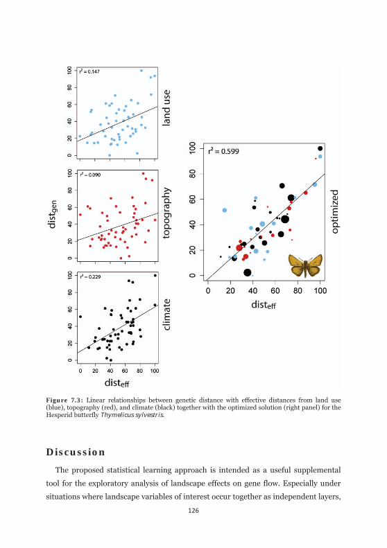
126
Figure 7.3: Linear relationships between genetic distance with effective distances from land use (blue), topography (red), and climate (black) together with the optimized solution (right panel) for the Hesperid butterfly Thymelicus sylvestris.
Discussion
The proposed statistical learning approach is intended as a useful supplemental
tool for the exploratory analysis of landscape effects on gene flow. Especially under
situations where landscape variables of interest occur together as independent layers,
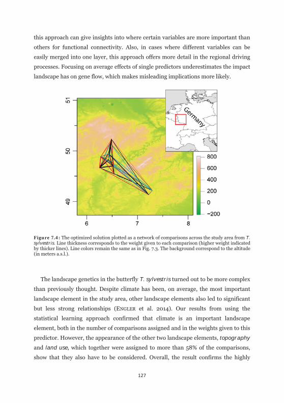
127
this approach can give insights into where certain variables are more important than
others for functional connectivity. Also, in cases where different variables can be
easily merged into one layer, this approach offers more detail in the regional driving
processes. Focusing on average effects of single predictors underestimates the impact
landscape has on gene flow, which makes misleading implications more likely.
Figure 7.4: The optimized solution plotted as a network of comparisons across the study area from T. sylvestris. Line thickness corresponds to the weight given to each comparison (higher weight indicated by thicker lines). Line colors remain the same as in Fig. 7.3. The background correspond to the altitude (in meters a.s.l.).
The landscape genetics in the butterfly T. sylvestris turned out to be more complex
than previously thought. Despite climate has been, on average, the most important
landscape element in the study area, other landscape elements also led to significant
but less strong relationships (ENGLER et al. 2014). Our results from using the
statistical learning approach confirmed that climate is an important landscape
element, both in the number of comparisons assigned and in the weights given to this
predictor. However, the appearance of the other two landscape elements, topography
and land use, which together were assigned to more than 58% of the comparisons,
show that they also have to be considered. Overall, the result confirms the highly
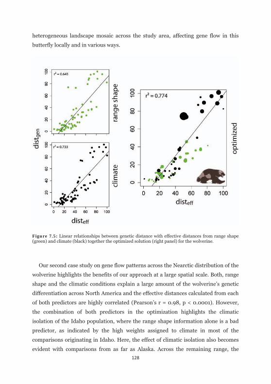
128
heterogeneous landscape mosaic across the study area, affecting gene flow in this
butterfly locally and in various ways.
Figure 7.5: Linear relationships between genetic distance with effective distances from range shape (green) and climate (black) together the optimized solution (right panel) for the wolverine.
Our second case study on gene flow patterns across the Nearctic distribution of the
wolverine highlights the benefits of our approach at a large spatial scale. Both, range
shape and the climatic conditions explain a large amount of the wolverine’s genetic
differentiation across North America and the effective distances calculated from each
of both predictors are highly correlated (Pearson’s r = 0.98, p < 0.0001). However,
the combination of both predictors in the optimization highlights the climatic
isolation of the Idaho population, where the range shape information alone is a bad
predictor, as indicated by the high weights assigned to climate in most of the
comparisons originating in Idaho. Here, the effect of climatic isolation also becomes
evident with comparisons from as far as Alaska. Across the remaining range, the
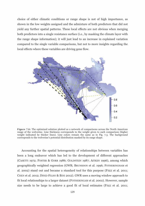
129
choice of either climatic conditions or range shape is not of high importance, as
shown in the low weights assigned and the admixture of both predictors that did not
yield any further spatial patterns. These local effects are not obvious when merging
both predictors into a single resistance surface (i.e., by masking the climate layer with
the range shape information); it will just lead to an increase in explained variation
compared to the single variable comparisons, but not to more insights regarding the
local effects where these variables are driving gene flow.
Figure 7.6: The optimized solution plotted as a network of comparisons across the North American range of the wolverine. Line thickness corresponds to the weight given to each comparison (higher weight indicated by thicker lines). Line colors remain the same as in Fig. 7.3. The background corresponds to the wolverine’s potential distribution masked by its range shape.
Accounting for the spatial heterogeneity of relationships between variables has
been a long endeavor which has led to the development of different approaches
(CASETTI 1972; FOSTER & GORR 1986; GOLDSTEIN 1987; AITKEN 1996), among which
geographically weighted regression (GWR; BRUNSDON et al. 1996; FOTHERINGHAM et
al. 2002) stand out and became a standard tool for this purpose (PÁEZ et al. 2011;
CHEN et al. 2012; DINIZ-FILHO & BINI 2012). GWR uses a moving window approach to
fit local relationships to a larger dataset (FOTHERINGAM et al. 2002). However, sample
size needs to be large to achieve a good fit of local estimates (PÁEZ et al. 2011;
130
DEVKOTA et al. 2014). In landscape genetics, large sample sizes by means of locations
sampled (i.e. n 160; PÁEZ et al. 2011) are rarely met, even though attempts had been
made to use GWR in that way (e.g., SPEAR et al. 2012). As opposed to GWR, our
statistical learning approach led to outcomes of local driving and varying landscape
patterns—even under sample sizes that are typical in landscape genetics. Our
approach therefore allows characterizing the landscape patterns that cause spatial
nonstationarity in genetic differentiation under situations, where GWR cannot.
Recently, DUFORET-FREBOURG & BLUM (2014) proposed a method that assesses
spatial nonstationarity in IBD patterns using Bayesian kriging and highlight its
extension to landscape genetics. In particular, this approach detects genetic
discontinuities, where local genetic differentiation is larger (or smaller) than a
baseline estimate of genetic differentiation over the entire study area (DUFORET-
FREBOURG & BLUM 2014). However, the approach did not correlate these genetic
discontinuities to certain landscape elements afterwards, and thus relied entirely on
the available methods in landscape genetics to link these outcomes to landscape
elements. In consequence, even though spatial nonstationarity of genetic
differentiation can be detected, it will be correlated again to approaches that focus on
the average effect of single landscape elements instead of linking them directly to the
detected discontinuities. Hence, the landscape patterns identified using our
optimization technique can offer potential explanations to the genetic discontinuities
detected in Bayesian kriging and serve as an important supplemental tool in this
regard.
In conclusion, our new approach highlights where specific landscape elements are
driving gene flow at a local scale and by this find a solution for each single
comparison. This contrasts with most efforts in landscape genetics which focus on the
quantification of average effects only. The approach is of particular interest when
results are used for management recommendations in conservation and questions the
projection of results of landscape genetic studies onto different regions and spatial
scales. By this, we recommend its use as an explanatory tool in landscape genetics
that can supplement the reliability of average effects and account for spatial
nonstationarity in migration rates. To this end, we hope that this approach will be
implemented in a wide range of methods that correlate genetic distances with
effective distances to fully account for the dynamic nature of the landscape.
131
Supplementary material
A climate SDM for the wolverine
Species data
We compiled wolverine occurrence information in a query at the Global
Biodiversity Information Facility (GBIF, www.gbif.org, retrieved 08/2014), leading to
a total of >15,000 records. After removing records without spatial reference,
duplicates, or records outside the study area, 500 presence locations remained. These
localities were spatially biased towards Alaska (317 records; 63.4% of all records) and
Nunavut/Canada (138 records; 27.6% of all records). As spatial sampling bias is well
known to negatively affect SDM results due to uneven sampling density (e.g., SYFERT
et al. 2013; KRAMER-SCHADT et al. 2013; FOURCADE et al. 2014), we generated a subset
of 100 records by using a hierarchical cluster analysis over the geographic space (i.e.,
by using lat/long coordinates as explanatory variables) and randomly selected one
record for each of the predefined solution of 100 clusters. The cluster analysis was
performed in SPSS 14.0.
Environmental variables
We used a subset of the 19 bioclimatic variables obtained from the WorldClim
database (Vers. 1.4.; HIJMANS et al. 2005) at a spatial resolution of 30 arc seconds. As
the wolverine’s range is strongly delimited by the retainment of snow in spring
(MAGOUN & COPELAND 1998; AUBRY et al. 2007; COPELAND et al. 2010) and to avoid
model overparameterization due to the inclusion of too many predictor variables in
the species distribution model (HEIKKINEN et al. 2006), we reduced the initial set of
19 predictors to a subset of six predictors that were assumed to be the most
biologically relevant to the species (Table 7.S1).
Modeling framework
For the SDM, we used the program MAXENT (vers. 3.3.3k; PHILLIPS et al. 2006), a
machine learning algorithm based on the principles of maximum entropy (ELITH et
al. 2011). MAXENT frequently outperforms other competing methods and has been
shown to be robust under complex scenarios and low numbers of presence records

132
(HERNANDEZ et al. 2006, ELITH et al. 2006, WISZ et al. 2008). We apply SDMs using
auto features and the logistic output format after 100 repetitive runs where we
randomly subsampled 30% of the occurrence data for model testing. The resulting
suitability maps were reprojected to an equidistant UTM projection at 1km² spatial
resolution using the RASTER package in R (HIJMANS & VAN ETTEN 2012).
Table 7.S1: Predictors used for conducting the SDM for the wolverine.
Worldclim code MeaningBio1 Annual mean temperature Bio4 Temperature seasonality Bio5 Maximum temperature of warmest month Bio8 Mean temperature of wettest quarter Bio12 Annual precipitation Bio15 Precipitation seasonality

133

134

135
PART CIMPROVING SDMS USING CONTEMPORARY GENETIC
INFORMATION

136

137
CHAPTER 8
Genes to the niche! How contemporary DNA can help to refine
niche theory for predicting range dynamics in the
Anthropocene
“The north, south, east, and west boundaries of a species’ range tell us very little about what is happening inside…”
ROBERT H. MACARTHUR

138
The work was conducted in collaboration with NIKO BALKENHOL from the Wildlife Science Department, University of Göttingen and CATHERINE H GRAHAM from the Department of Ecology and Evolution, Stony Brook University.
139
Niche models, theory, and the recent integration of genetic information
The technological revolution in the past 25 years now allows the analysis of species
occurrence information in completely novel ways. Correlative environmental niche
models (ENM) that link occurrence information to a set of environmental variables
appeared as a central tool in this regard, with applications covering a wide array of
disciplines in ecology and evolution (PETERSON & VIEGLAIS 2001; GUISAN & THULLIER
2005; KOZAK et al. 2008; FRANKLIN 2009; PETERSON et al. 2011). These models are
based on Hutchinson’s niche concept which assumes that species niches are
constrained by a combination of environmental tolerances and biotic interactions
(Box 1; SOBERÓN 2007; 2010; 2014; WARREN 2012; 2013). Use of this concept as a
basis for ENMs (hereafter referred to as ENM concept), has been criticized (JIMÉNEZ-
VALVERDE et al. 2008; MCINERNY & ETIENNE 2013) and recent studies suggest that it
should be refined to include more biological detail (e.g., HOLT 2009). To this end,
researchers have begun to integrate mechanistic (KEARNEY & PORTER 2009; DORMAN
et al. 2012; CABRAL & KREFT 2012) and genetic information into ENMs.
Phylogeographic (CHAN et al. 2011; ALVARADO-SERRANO & KNOWLES 2014), and
landscape genetic research (MANEL& HOLDEREGGER 2013; ENGLER et al. 2013)
increasingly use ENMs to explore genetic patterns. In addition, the potential of
genetic data for improving ENM predictions has been highlighted (HOLT 2009;
SCOBLE & LOWE 2010; FORDHAM et al. 2014; GOTELLI & STANTON-GEDDES 2015).
However, we currently lack a conceptual framework that integrates population
genetic information into the ENM concept. Here, we explore a conceptual framework
that demonstrates how genetic information can be used to enhance our
understanding of range dynamics and refer, where available, to specific examples
from the scientific literature. In particular, we show how integrating genetic
information into ENM permits a more holistic view of niche theory and discuss
limitations associated with how the ENM concept is currently being used. We assert
that in order to address the modeling challenges in the era of the Anthropocene,
where habitat fragmentation, biotic invasions, and climate change are major human-
caused threats to global biodiversity, use of the ENM concept should be refined. In
addition, we provide recommendations for the design of integrated studies using
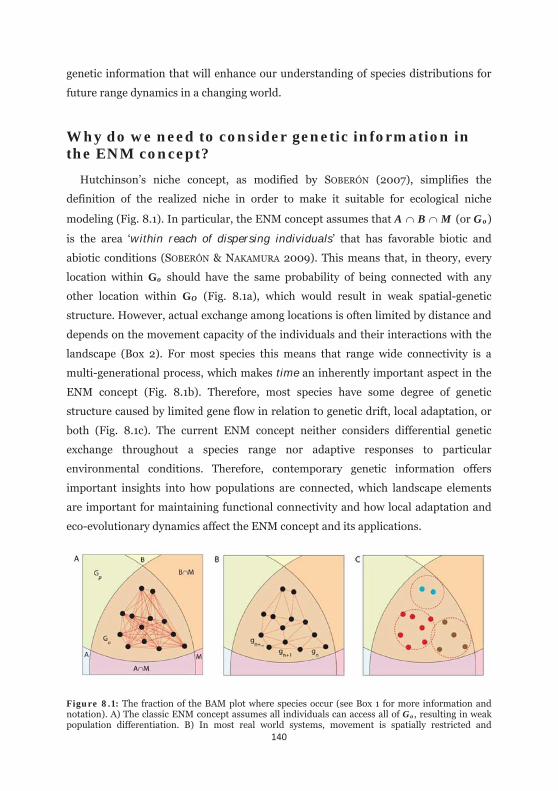
140
genetic information that will enhance our understanding of species distributions for
future range dynamics in a changing world.
Why do we need to consider genetic information in the ENM concept?
Hutchinson’s niche concept, as modified by SOBERÓN (2007), simplifies the
definition of the realized niche in order to make it suitable for ecological niche
modeling (Fig. 8.1). In particular, the ENM concept assumes that A B M (or Go)
is the area ‘within reach of dispersing individuals’ that has favorable biotic and
abiotic conditions (SOBERÓN & NAKAMURA 2009). This means that, in theory, every
location within Go should have the same probability of being connected with any
other location within GO (Fig. 8.1a), which would result in weak spatial-genetic
structure. However, actual exchange among locations is often limited by distance and
depends on the movement capacity of the individuals and their interactions with the
landscape (Box 2). For most species this means that range wide connectivity is a
multi-generational process, which makes time an inherently important aspect in the
ENM concept (Fig. 8.1b). Therefore, most species have some degree of genetic
structure caused by limited gene flow in relation to genetic drift, local adaptation, or
both (Fig. 8.1c). The current ENM concept neither considers differential genetic
exchange throughout a species range nor adaptive responses to particular
environmental conditions. Therefore, contemporary genetic information offers
important insights into how populations are connected, which landscape elements
are important for maintaining functional connectivity and how local adaptation and
eco-evolutionary dynamics affect the ENM concept and its applications.
Figure 8.1: The fraction of the BAM plot where species occur (see Box 1 for more information and notation). A) The classic ENM concept assumes all individuals can access all of Go, resulting in weak population differentiation. B) In most real world systems, movement is spatially restricted and
141
influenced by landscape heterogeneity, which makes the exchange across Go a multi-generational process (gn, gn+1, gn+…). In consequence, genetic differentiation becomes likely because of restricted gene flow. C) Environmental factors can exert selection pressures that can counteract gene flow, leading to spatial genetic structure.
Integrating genetic information to understand the processes behind range dynamic patterns
To highlight how genetic information can refine niche theory, we focus on five
broad aspects: (i) gene flow, (ii) spatial genetic structure, (iii) density blocking, (iv)
hybridization, and (v) source-sink dynamics (Fig. 8.B1.1b). While these processes are
not fully independent from each other, we focus on each one separately, starting with
those directly acting at the level of the occupied realized niche Go, followed by
processes acting during colonization (expansion of Go) and finally source-sink
dynamics acting in the original or expanded Go.
Gene flow and functional connectivity: Exchange within Go is limited
Gene flow estimates can be used to quantify functional connectivity of landscapes.
The ENM concept assumes that all occurrences within Go ‘have been accessible to the
species since some arbitrary point in time’ (SOBERÓN 2007: 1120). As such, Go is
treated as a continuous and homogeneous surface which allows exchange among all
localities within Go with the same probability in the long term (Fig. 8.2a). Following
this assumption, most EMNs assume that species can disperse to regions where
environmental conditions are suitable. This assumption is likely violated because
many landscape genetic studies show that environmental heterogeneity can strongly
influence dispersal and resulting population connectivity (MANEL & HOLDEREGGER
2013; DYER 2015b; WAITS et al. 2015). Consequently, ENMs based on climate data
may not render spatial occurrence patterns needed for identifying the processes
influencing species distributions. However, identifying the processes affecting
distributional patterns is needed to mitigate the influence of climate change on
populations and species (Box 2). For instance, ENGLER et al. (2013) showed that
ENMs based on climate adequately predicted potential distributions for three
congeneric butterflies (Genus: Thymelicus). However when related to gene flow,
climate was identified as an important predictor for functional connectivity in only
one species, while being a poor predictor for the other two (ENGLER et al. 2013). The

142
current ENM concept does not consider the importance of functional connectivity for
range dynamics and how this interplay is affected by increasing habitat
fragmentation (e.g., TRAVIS 2003; HOF et al. 2011). This is of particular concern, since
habitat loss is assumed to more strongly impact species persistence than climate
change (STEFFEN et al. 2015 a;b).
Spatial genetic structure: Go is more complex and diverse
Species can show spatial genetic structure due to limited gene flow and adaptation
to local environmental conditions (Fig. 8.1c). Local adaptation actively counteracts
the admixing effect of gene flow and can occur at different spatial scales (RICHARDSON
et al. 2014). This can lead to the formation of geographically distinct genetic demes,
which remain largely unconsidered in the ENM concept and the definition of Go (Fig.
8.1c).
Recently, studies have begun to incorporate information on spatially separated
genetic demes into EMNs on coarse spatial scales. The consideration of genetic
demes yields more accurate predictions of species distributions than the common
practice of pooling occurrence records at the species level (PETERSON & HOLT 2003;
PEARMAN et al. 2010; VALLADARES et al. 2014). For instance, GONZALEZ et al. (2011)
refined their prediction of the potential distribution of old field mice (Peromyscus
polionotus) after accounting for differences in bioclimatic niche space used by
different subspecies. Use of genetic information may be particularly important for
generating future projections if unique genetic demes are considered (ONEY et al.
2013). VALLADARES et al. (2014) demonstrated that forecasts incorporating intra-
specific variation (due to local adaptations) showed more dramatic declines than
when occurrences were pooled at the species level. These examples suggest that
incorporating spatial genetic structure can have profound effects on the niche space
estimated, potentially reducing the risk of overestimation of Go (Box 2).
Overestimation of the niche might be particularly problematic if the niche delimiting
factors are not the same among the genetic demes (e.g., ONEY et al. 2013), or if
impacts of environmental heterogeneity on functional connectivity vary across the
geographic range of a species (e.g., SHORT BULL et al. 2011; DUDANIEC et al. 2012;
LEVY et al. 2013). To accommodate within-species variation in environmental
143
requirements, separate analyses should be conducted with reference to the spatial
genetic structure found at finer scales.
Density blocking: Expansion may not be a simple projection of the conditions across the entire native range
Species with spatial genetic structures might behave in very different ways if they
colonize new regions. Recently, the term density blocking was introduced to
summarize interdependent priority effects such as gene/allele-surfing, competitive
exclusion, and leading edge colonization (WATERS et al. 2013). These density driven
priority effects, imprinted in genetic patterns, are crucial for our understanding of
colonization events such as range expansions and biological invasions. Including this
information into niche models will result in better forecasts and allow for clearer
signals of niche stasis vs. niche evolution (Box 3).
Given that a species range within Go is often genetically structured and exchange is
not equal throughout, density blocking should be considered to better understand
and predict expansions of Go. Natural range expansions normally occur into areas in
A or B of the BAM diagram that are adjacent to Go and become suitable and are thus
colonized from source populations along the range edge (i.e., leading edge
colonization, HEWITT 1996). In biotic invasions however, expansions are expected to
result mostly in the occupation of Gp due to human mediated crossing of macro-scale
barriers (i.e., an artificial expansion of M). While these two mechanisms likely
represent the most common ways in which species expand their range, questions
remain as to where within Go founders come from and what their genetic
characteristics are. For instance, leading edge colonization results in density-driven
priority effects that favor local genotypes over those that arrive later, and more
sporadically, from more distant locations (WATERS et al. 2013). In addition to pure
priority effects that dominate leading edge colonization, it is possible that local
adaptation may favor immigrants from closer populations more compared to those
from distant parts of the range. Under local adaptation, different genetic demes
should be detectable in environmental space. In contrast, genetic differentiation due
to density blocking does not necessarily coincide with a strong separation in
environmental space (Box 3). This information is crucial for interpreting the degree
of niche overlap between original ranges and areas of range expansion. If genetic
144
demes are separated in E-space, then comparisons should be made just with the
genetic demes involved in the expansion because pooling deems at the species level
will lead to lower estimated niche overlap that do not accurately reflect true niche
overlap. As a result a false signal of niche evolution could appear where there is a high
level of niche stasis.
Hybridization: expansion by accessing new niche space
Hybridization appears above and below the species level and its prevalence often
increases during accelerating rates of faunal exchange by human activities (THOMAS
2013). Hybridization between members of different genetic demes can lead to an
expansion of realized niche space. Realized niches can be complex in species with
spatial genetic structure (Box 2). If genetic demes come into secondary contact
(either by natural range expansions or by human-mediated translocations), their
distinct realized niches in E-space might expand due to hybridization and by this
enlarge total realized niche space.
Hybridization can lead to an increased adaptive potential, which in turn, can allow
the colonization of formerly unsuitable habitat. While hybridization is common in
natural populations (ARNOLD 1997; SCHWENK et al. 2008) studying its role in niche
expansion can be difficult because hybridization is often an on-going long term
process. In contrast, in biological invasions members of different genetic demes are
brought into secondary contact providing a short-term perspective on how
hybridization might influence species niches. Compared to native populations, a
surprisingly high genetic diversity can be found in different populations of invasive
species in both plants (LAVERGNE & MOLOFSKY 2007) and animals (KOLBE et al. 2004;
2007; DETWILER & CRISCIONE 2014). Comparative population genetic studies between
native and invasive ranges are needed to better understand how niches are altered
during biological invasions which might explain invasion success as well as further
spread. In particular, such information could contribute to our understanding of
whether niche evolution, niche stasis, or niche plasticity influences invasion success
(Box 3).
145
Source-sink dynamics: beyond classical definitions and implications
Populations are rarely continuous but usually are patchily distributed in
geographic space, often as part of a metapopulation network (HARRISON 1991; HANSKI
1999). Depending the landscape heterogeneity, patch size and connectivity,
populations can range from large and productive source populations to small sink
populations that need immigration from sources to persist. These source-sink
dynamics are crucial for landscape ecology and meta-population theory and their
implications for niche theory and the ENM concept have long been recognized
(PULLIAM 1988; 2000; SOBERÓN 2007).
SOBERÓN (2007) applied the source-sink area of distribution as formulated by
PULLIAM (2000) to the ENM concept as the area delimited by M, where sources were
located within Go, and sinks within the remaining area of M. However, the
integration of source-sink dynamics in classical niche modeling approaches suffers
from three main problems. First, information on the source-sink status is lacking for
most occurrences. This makes assignment of an occurrence record to either Go or the
remaining M difficult. Second, the source-sink status at a specific location might
change over time (JOHNSON 2004). Hence, an occurrence record might be within Go
in some years but outside in others. Finally, depending on the underlying processes
behind source-sink dynamics, their impact on model predictions depends on the
choice and spatial scale of the environmental predictors used for modeling (DIEZ &
GILADI 2009). Thus, whether a location is within Go depends on the variables
considered.
Genetic measures of asymmetrical migration (i.e., gene flow) and effective
population sizes (Ne) can be used to characterize source populations as those with
high emigration and Ne , while sink populations should show high immigration and
low Ne (e.g., HUSEMANN et al. 2015). After this characterization, overlaps in E-space
can be calculated and compared against locations assigned to as either sources or
sinks. If sources and sinks are distinct in environmental space, sinks should be
excluded from ENMs, as they overestimate Go which has been seen as problematic
(HOLT 2009; PAGEL & SCHURR 2012; SCHURR et al. 2012). If, however, no distinction
can be made between these two states based on environmental predictors, the
categorization as made in SOBERÓN (2007) does not affect ENMs, as the niche space
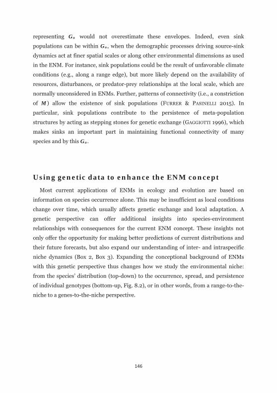
146
representing Go would not overestimate these envelopes. Indeed, even sink
populations can be within Go, when the demographic processes driving source-sink
dynamics act at finer spatial scales or along other environmental dimensions as used
in the ENM. For instance, sink populations could be the result of unfavorable climate
conditions (e.g., along a range edge), but more likely depend on the availability of
resources, disturbances, or predator-prey relationships at the local scale, which are
normally unconsidered in ENMs. Further, patterns of connectivity (i.e., a constriction
of M) allow the existence of sink populations (FURRER & PASINELLI 2015). In
particular, sink populations contribute to the persistence of meta-population
structures by acting as stepping stones for genetic exchange (GAGGIOTTI 1996), which
makes sinks an important part in maintaining functional connectivity of many
species and by this Go.
Using genetic data to enhance the ENM concept
Most current applications of ENMs in ecology and evolution are based on
information on species occurrence alone. This may be insufficient as local conditions
change over time, which usually affects genetic exchange and local adaptation. A
genetic perspective can offer additional insights into species-environment
relationships with consequences for the current ENM concept. These insights not
only offer the opportunity for making better predictions of current distributions and
their future forecasts, but also expand our understanding of inter- and intraspecific
niche dynamics (Box 2, Box 3). Expanding the conceptional background of ENMs
with this genetic perspective thus changes how we study the environmental niche:
from the species’ distribution (top-down) to the occurrence, spread, and persistence
of individual genotypes (bottom-up, Fig. 8.2), or in other words, from a range-to-the-
niche to a genes-to-the-niche perspective.
147
Figure 8.2: Expanding the ENM concept with genetic information. The classical ENM concept is based on a distribution-based perspective using occurrence records to infer the realized niche, as a subset of the fundamental niche. The eco-physiological limits of the fundamental niche are assumed to change slowly via niche evolution, while the realized niche is more plastic in its ability to change within the limits set by the fundamental niche. In contrast the genotype-based perspective uses information on standing genetic variation which frames a genotypic niche that is bound by evolutionary edges. These edges can change over long timescales when novel mutations expand the currently known standing genetic variation and are favored by selection. From this bottom-up perspective, we can assess the realized niche using information on spatial genetic structure and functional connectivity.
The genes-to-the-niche perspective replaces the static fundamental niche by a
more dynamic genotypic niche, which allows for a more detailed view of the realized
niche and its geographic distribution Go (Fig. 8.2). Overestimation of Go may be
prevented when taking locally adapted genetic demes and functional connectivity
within and among these demes into account. This perspective also allows us to
consider how the fundamental niche might change through time to influence species
distributions. Characterization of the fundamental niche using a species’ eco-
physiological limits is one of the cornerstones in the ENM concept (SOBERÓN 2007).
Following this perspective, niche evolution is considered to act over long time scales
(NOGUÉS-BRAVO 2009). However, this assumption is not always supported with
genetic data, indicating that a more dynamic ENM concept may be required to
predict range dynamics. Since the interplay of intraspecific local adaptation with
environmental conditions (SAVOLAINEN et al. 2013) affects Go in many ways, the
fundamental niche could be expanded to consider standing genetic variation
(HENDRY 2013). Experimental studies indicate that species can adapt rapidly to
148
climatic change, even within a few generations (e.g., SKELLY et al. 2007). These
adaptations mostly result from standing genetic variation, due to changes of allele
frequencies, while new genetic variation from novel mutations are less frequent and
take longer to manifest in phenotypes (HENDRY 2013). This makes standing genetic
variation a crucial part of eco-evolutionary dynamics, where environmental changes
induce evolutionary responses that lead to short-term adaptations. When rapid
evolution is considered in the ENM concept, the fundamental niche becomes a
dynamic entity that is able to change over very short time scales. By this, standing
genetic variation could push the static concept of the fundamental niche towards a
dynamic “genotypic” niche defined by evolutionary edges that allows some flexibility
due to rapid adaption to environmental change (Fig. 8.2).
The dynamic ENM concept we propose here is also important from a conservation
perspective. Local adaptation leads to spatial heterogeneity of a species’ standing
genetic variation. This heterogeneity can be the result of different adaptive strategies
to environmental conditions across a species’ range (BOTERO et al. 2015). Even
though these strategies can be flexible against environmental change, they can cross
evolutionary tipping points where one adaptive strategy is replaced by another one
(BOTERO et al. 2015). Crossing these tipping points can have profound negative
consequences, driving affected populations to extinction if the adaptive strategy they
follow is no longer beneficial under the changing conditions (BOTERO et al. 2015). In
the context of human made environmental change, populations can be forced
towards those tipping points due to increased speed and magnitude of environmental
change. In order to facilitate rapid adaptation, not only species but also the genetic
variation within these species need to be conserved (MORITZ 1994; CRANDALL et al.
2000; PALSBØLL et al. 2007; SCHWARTZ et al. 2007). Consequently, a dynamic ENM
concept based on a genotypic niche can be an important step towards better
conservation in the Anthropocene, as it provides an eco-evolutionary complement to
the currently prevailing ENM predictions based on eco-physiological limits.
149
Concluding remarks
Contemporary genetic information can improve niche theory in many ways which
will allow generation of better ENMs that link to eco-evolutionary dynamics. The
proposed dynamic perspective on the ENM concept accounts for losses of standing
genetic variation due to human activities. Applying this ENM concept requires better
coverage of genetic information across multiple spatial and taxonomic scales. Given
the increasingly (cost) effective techniques for assessing neutral and adaptive genetic
variation in non-model organisms, the genes-to-the-niche perspective in a dynamic
ENM concept allows to enter new research topics to face the challenges of a rapidly
changing world.
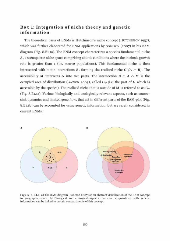
150
Box 1: Integration of niche theory and genetic information
The theoretical basis of ENMs is Hutchinson’s niche concept (HUTCHINSON 1957),
which was further elaborated for ENM applications by SOBERÓN (2007) in his BAM
diagram (Fig. 8.B1.1a). The ENM concept characterizes a species fundamental niche
A, a scenopoetic niche space comprising abiotic conditions where the intrinsic growth
rate is greater than 1 (i.e. source populations). This fundamental niche is then
intersected with biotic interactions B, forming the realized niche G (A B). The
accessibility M intersects G into two parts. The intersection B A M is the
occupied area of distribution (GASTON 2003), called GO (i.e. the part of G which is
accessible by the species). The realized niche that is outside of M is referred to as GP
(Fig. 8.B1.1a). Various biologically and ecologically relevant aspects, such as source-
sink dynamics and limited gene flow, that act in different parts of the BAM-plot (Fig.
8.B1.1b) can be accounted for using genetic information, but are rarely considered in
current ENMs.
Figure 8.B1.1: a) The BAM diagram (Soberón 2007) as an abstract visualization of the ENM concept in geographic space. b) Biological and ecological aspects that can be quantified with genetic information can be linked to certain compartments of this concept.
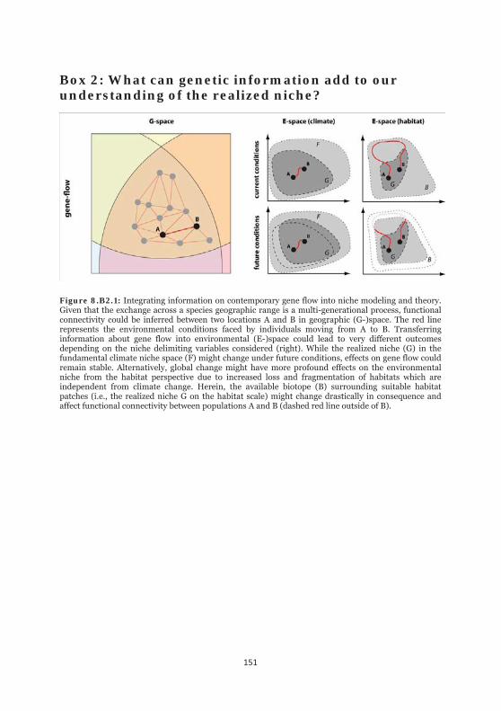
151
Box 2: What can genetic information add to our understanding of the realized niche?
Figure 8.B2.1: Integrating information on contemporary gene flow into niche modeling and theory. Given that the exchange across a species geographic range is a multi-generational process, functional connectivity could be inferred between two locations A and B in geographic (G-)space. The red line represents the environmental conditions faced by individuals moving from A to B. Transferring information about gene flow into environmental (E-)space could lead to very different outcomes depending on the niche delimiting variables considered (right). While the realized niche (G) in the fundamental climate niche space (F) might change under future conditions, effects on gene flow could remain stable. Alternatively, global change might have more profound effects on the environmental niche from the habitat perspective due to increased loss and fragmentation of habitats which are independent from climate change. Herein, the available biotope (B) surrounding suitable habitat patches (i.e., the realized niche G on the habitat scale) might change drastically in consequence and affect functional connectivity between populations A and B (dashed red line outside of B).
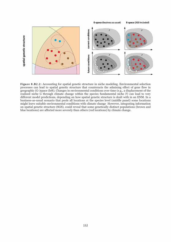
152
Figure 8.B2.2: Accounting for spatial genetic structure in niche modeling. Environmental selection processes can lead to spatial genetic structure that counteracts the admixing effect of gene flow in geographic (G-)space (left). Changes in environmental conditions over time (e.g., a displacement of the realized niche G through climate change within the species fundamental niche F) can lead to very different model predictions, depending on how spatial genetic structure is dealt with in an ENM. In a business-as-usual scenario that pools all locations at the species level (middle panel) some locations might leave suitable environmental conditions with climate change However, integrating information on spatial genetic structure (SGS), could reveal that some genetically distinct populations (brown and blue locations) are affected more severely than others (red locations) by climate change.
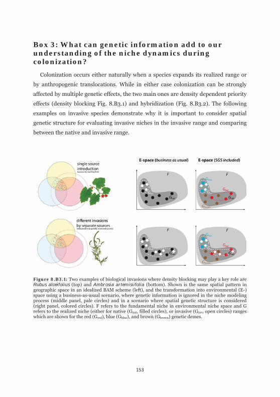
153
Box 3: What can genetic information add to our understanding of the niche dynamics during colonization?
Colonization occurs either naturally when a species expands its realized range or
by anthropogenic translocations. While in either case colonization can be strongly
affected by multiple genetic effects, the two main ones are density dependent priority
effects (density blocking Fig. 8.B3.1) and hybridization (Fig. 8.B3.2). The following
examples on invasive species demonstrate why it is important to consider spatial
genetic structure for evaluating invasive niches in the invasive range and comparing
between the native and invasive range.
Figure 8.B3.1: Two examples of biological invasions where density blocking may play a key role are Rubus alceifolius (top) and Ambrosia artemisiifolia (bottom). Shown is the same spatial pattern in geographic space in an idealized BAM scheme (left), and the transformation into environmental (E-) space using a business-as-usual scenario, where genetic information is ignored in the niche modeling process (middle panel, pale circles) and in a scenario where spatial genetic structure is considered (right panel, colored circles). F refers to the fundamental niche in environmental niche space and G refers to the realized niche (either for native (Gnat, filled circles), or invasive (Ginv, open circles) ranges which are shown for the red (Gred), blue (Gblue), and brown (Gbrown) genetic demes.
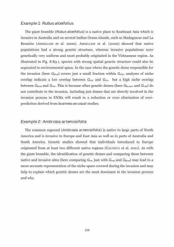
154
Example 1: Rubus alceifolius
The giant bramble (Rubus alceifolius) is a native plant to Southeast Asia which is
invasive in Australia and on several Indian Ocean islands, such as Madagascar and La
Reunión (AMSELLEM et al. 2000). AMSELLEM et al. (2000) showed that native
populations had a strong genetic structure, whereas invasive populations were
genetically very uniform and most probably originated in the Vietnamese region. As
illustrated in Fig. 8.B3.1, species with strong spatial genetic structure could also be
separated in environmental space. In the case where the genetic deme responsible for
the invasion (here Gblue) covers just a small fraction within Gnat, analyses of niche
overlap indicate a low overlap between Gnat and Ginv but a high niche overlap
between Gblue and Ginv. This is because other genetic demes (here Gbrown and Gred) do
not contribute to the invasion. Including just demes that are directly involved in the
invasion process in ENMs will result in a reduction or even elimination of over-
prediction derived from business-as-usual studies.
Example 2: Ambrosia artemisiifolia
The common ragweed (Ambrosia artemisiifolia) is native to large parts of North
America and is invasive in Europe and East Asia as well as in parts of Australia and
South America. Genetic studies showed that individuals introduced to Europe
originated from at least two different native regions (GAUDEUL et al. 2011). As with
the giant bramble, the identification of genetic demes and comparing these between
native and invasive sites (here comparing Ginv just with Gred and Gblue) may lead to a
more accurate representation of the niche space covered during the invasion and may
help to explain which genetic demes are the most dominant in the invasion process
and why.
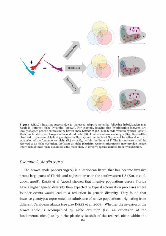
155
Figure 8.B3.2: Invasion success due to increased adaptive potential following hybridization may result in different niche dynamics (arrows). For example, imagine that hybridization between two locally adapted genetic entities in the brown anole (Anolis sagrei, blue & red) result in hybrids (violet). Under niche stasis, no changes in the realized niche (G) of native and invasive ranges (Gnat, Ginv) will be observed. Expansion of hybrid genotypes in Ginv beyond the limits of Gnat, could be either due to an expansion of the fundamental niche (Fn) or of Ginv within the limits of F. The former case would be referred to as niche evolution, the latter as niche plasticity. Genetic information may provide insight into which of these niche dynamics is the most likely in invasive species derived from hybridization.
Example 3: Anolis sagrei
The brown anole (Anolis sagrei) is a Caribbean lizard that has become invasive
across large parts of Florida and adjacent areas in the southwestern US (KOLBE et al.
2004; 2008). KOLBE et al (2004) showed that invasive populations across Florida
have a higher genetic diversity than expected by typical colonization processes where
founder events would lead to a reduction in genetic diversity. They found that
invasive genotypes represented an admixture of native populations originating from
different Caribbean islands (see also KOLBE et al. 2008). Whether the invasion of the
brown anole is accompanied by niche evolution (i.e., an expansion of the
fundamental niche) or by niche plasticity (a shift of the realized niche within the

156
constraints of the fundamental niche) is yet unclear. A study comparing
environmental niches between native and invasive ranges (ANGETTER et al. 2011)
identified niche shifts along some climatic predictors, even though possible local
environmental differences among native populations, that could relate to the genetic
patterns detected, were not taken into account. Additional genetic and genomic
studies focusing on adaptive evolution combined with niche models at finer
taxonomic levels would make this species an ideal system to study niche dynamics
during invasion.

157

158

159
GENERAL DISCUSSION
“We are approaching a new age of synthesis. Knowledge cannot be merely a degree or a skill… It demands a broader vision, capabilities in critical thinking and logical deduction without which we cannot have constructive progress.”
LI KA-SHING

160

161
The general subject of my thesis was to tie together species distribution models
with connectivity models to potential connectivity models (PCMs) to explore spatial
exchange among populations in a standardized manner. Without additional genetic
information, this synergy of methods is able to assess the potential connectivity of
habitats for matrix-sensitive species at very fine spatial scales. These exploratory
analyses can be very helpful tools in environmental planning, as they disentangle
global trends from local effects and generate easily-legible maps to inform
consultants, managers and stakeholders, alike. Furthermore, when combined with
genetic information, this approach can fully unfold its potential. Primarily, we can
learn how the environment affects a species’ functional connectivity to answer
different ecological questions. In addition, we can functionally evaluate model
settings and their underlying theory, thus improving our understandings and
assumptions of species-environment relationships from the conceptual perspective.
The necessity to include standard connectivity assessments in conservation management and policy
Conservation biology is changing its mindset from establishing static and isolated
protected areas, to designing dynamic conservation networks. In consequence,
connectivity conservation is emerging as a mature sub-discipline to explore the
dynamic ways to protect species under changing climatic conditions and
anthropogenic pressures (CROOKS & SANJAYAN 2006). Globally, most protected areas
are isolated within a highly modified landscape matrix by humans, preventing
exchange among sites and making at-site extinctions a lasting state (SEIFERLING et al.
2012). Moreover, when conditions change at the macro scale (e.g., climate),
maintaining connectivity at finer scales becomes more important than ever, affecting
not only which species to protect, but also the legal status of protected sites (e.g.,
RÖDDER & SCHULTE 2012). However, as shown and discussed in Part A of my thesis,
despite having an exemplary internationally coordinated legal regime for
environmental protection, the EU’s habitat directive and its accompanied Natura
2000 network of protected sites failed to stop biodiversity loss within the EU borders
(EEA 2010). Next to other improvements (HOCHKIRCH et al. 2013), we require an
implementation of current knowledge on connectivity conservation to improve the
existing infrastructure of Natura 2000 sites (Chapter 3). This includes strategies to
effectively compensate for at-site losses due to changing climatic regimes (Chapter 4),
162
and the development and implementation of methodological frameworks as
preventive measures in environmental planning (Chapter 5).
The proposed PCM framework can add to our understanding of how connectivity
affects the observed patterns of changing distributions and can give spatially-explicit
information and guidance; it will provide insight on where future developments will
likely affect species. In particular, Chapter 4 has shown that declining trends in
specialist species appear in protected and unprotected sites, alike. Even though these
changes in butterfly communities were more controlled at protected sites in contrast
to more stochastic changes in unmanaged and unprotected fallow grounds, both
communities changed from being species-rich to being generalist-dominated.
Detected differences in structural connectivity among protected and unprotected sites
were not responsible for the observed changes, nor did they lead to contrasting effects
in the results. Consequently, this means that environmental factors acting at spatial
scales above where connectivity among patches is important are likely to drive
species trends at the global to regional level and need to be considered for future
management, as well. Integrated studies assessing the effects at different spatial
scales—from range shifts due to climate change, to functional connectivity at the
habitat level—are therefore mandatory to fully understand and manage declining
species. To this end, there is an ongoing debate about the roles of these different
compartments in light of biological conservation, and that a focus on connectivity
alone cannot solve the problems we currently face (HOGSON et al. 2009; DOERR et al.
2011; HODGSON et al. 2011).
However, the reality of environmental planning—at least in Germany—is at the
opposite end of this argument; it largely overlooks estimating connectivity in
planning practices, but rather focuses on habitat quality instead. Here, tools such as
the proposed PCM framework can help to include connectivity as an additional
source of information in the planning process for matrix-sensitive species. As shown
in Chapter 5, maps of potential connectivity can be very helpful guides in highlighting
areas of well-connected local populations, as well as areas where populations are
isolated and might suffer from a higher extinction risk. This way, stakeholders and
planners can decide if compensatory measures can be helpful as long-term preventive
measures for isolated sites, or if these are simply acceptable to lose. To this end,
simulations based on such maps could be used to find out which populations are of
163
particular importance for maintaining the whole network, and which are not (e.g.,
RUBIO et al. 2015). Using habitat quality as a cornerstone in the evaluation of
assessed areas for possible future development contributes—in contrast to its
settlement areas—very little in explaining the connectivity of a species. Research has
shown that a species’ demands on habitat used for dispersal are lower than their
demands on habitat where they settle (HADDAD & TEWKSBURY 2005; DOERR et al.
2011). Standard assessment protocols used in environmental planning that focus on
habitat quality and abundance of individuals in species of concern therefore neglect
the role of connectivity, which increases the danger for more isolated populations in
the future. Maps highlighting potential connectivity in matrix-sensitive species can
therefore provide a more holistic assessment on the quality of areas under potential
future development.
Benefits and caveats of PCMs in landscape genetics
Landscape genetics is a steadily advancing and dynamic field which has led to the
development and application of a wide array of approaches during its first decade of
existence (MANEL et al. 2003, GUILLOT et al. 2005, MURPHY et al. 2008, BALKENHOL et
al. 2009, MANEL & HOLDEREGGER 2013). Our expectations for this field, however, are
manifold and strongly depend on the perspective of interest (BALKENHOL et al.
2015a). So was the initial definition of landscape genetics by MANEL et al. (2003),
focusing on “microevolutionary processes,” hence giving a strong emphasis on the
genetics, but were rather unspecific about the landscape (BALKENHOL et al. 2015b).
Over time, the definition has been extended (HOLDEREGGER & WAGNER 2006;
STORFER et al. 2007; BALKENHOL et al. 2015b), up to the point where landscape
genetics “[…] explicitly quantify the effects of landscape composition, configuration,
and matrix quality on microevolutionary processes, such as gene flow, drift, and
selection, using neutral and adaptive genetic data” (BALKENHOL et al. 2015b). While
the two compartments, “landscape” and “genes,” become equally entitled and refined
during this process, another issue arose: it heaves the entire field from a descriptive
to a quantitative discipline that allows the making of predictions on genetic aspects in
the wake of global change (e.g., JAY et al. 2012; WASSERMANN et al. 2012).
In my thesis, I devoted two chapters in Part B to questions related to landscape
genetics using PCMs, which supplements the range of available methods and allows
164
the quantification of the impact of landscape elements to gene flow. Yet, both
chapters seem to be opposing in their methodological philosophy beyond the use of
PCMs. While Chapter 6 compares the average effects of different landscape elements
to gene flow in a set of species, Chapter 7 questions this approach and instead goes
one step further of what was done in Chapter 6 to improve relationships between
landscape and genetic estimates. Nevertheless, both chapters are actually
complementary. Chapter 6 focuses on a general ecological question: do landscape
effects change with species specialization and mobility? Here, it was most important
to compare the average effects of the different landscape compartments among the
three species to draw general conclusions. In contrast, Chapter 7 asks how we can
incorporate landscape heterogeneity into comparisons between the landscape and
gene flow. The butterfly, Thymelicus sylvestris, was used in both chapters. Whether
the landscape - gene flow relationships focus on average effects of single landscape
elements, or on the combined effects of multiple landscape effects, climate remains as
the most important landscape variable for the species across the study area. Hence,
the general message was that the climatic conditions across the study area are
important for this species’ persistence. The approach used in Chapter 7, however,
added more details beyond the average effect; it showed where climate is driving this
correlation the most, and where other landscape elements might be locally more
important. This additional information could be very important to understand the
local drivers of gene flow and could help guide conservation efforts in species of
special concern. It further shows that results made in one area are hardly predictable
for other areas, which has been shown in a number of applications so far (SHORT BULL
et al. 2011; DUDANIEC et al. 2012; LEVY et al. 2013). The merit of Chapter 7 over those
studies is that the presented approach allows for one to visualize the driving factors
for each comparison, thereby laying the foundation for further research, asking more
precise questions, and establishing more robust sampling designs.
The PCM approach contributes to the development of landscape genetics and
accounts for some of the challenges raised by the community (summarized in
Balkenhol et al. 2015a), among which the approach as presented in Chapters 6 & 7
contributes to (1) a stronger emphasis on hypothesis testing (STORFER et al. 2007;
2010; CUSHMAN & LANDGUTH 2010; SEGELBACHER et al. 2010; MANEL & HOLDEREGGER
2013); (2) the use and development of predictive models for applications in
conservation and management (LANDGUTH & CUSHMAN 2010; MANEL et al. 2010;
165
SEGELBACHER et al. 2010; BOLLINGER et al. 2014); (3) the selection and understanding
of appropriate approaches and their assumptions (BALKENHOL et al. 2009; JAQUIÉRY
et al. 2011; WAGNER & FORTIN 2013); and (4) the understanding how scale and the
definition of the landscape influence the correlation of landscape effects on genetic
variation (CUSHMAN & LANDGUTH 2010; CUSHMAN et al. 2013).
Despite these contributions, there are limitations devoted to PCMs. The main
caveat is that the PCM approach does not include dispersal information in the
parameterization of the resistance surface. In cases where gene flow is estimated in
mobile species at very fine spatial scales, this predictive framework strongly depends
on the type and amount of presence records used to model habitat suitability. In the
case where these records would entirely represent breeding habitats, areas used for
dispersal gets ignored, but these are crucial for studying connectivity (SPEAR et al.
2010). This major critique however invalidates when the grain of environmental
predictors decreases and the spatial extent increases, or if occurrence information is
also available from dispersal habitats (i.e., from tracked individuals). In the former
case (when using climate data, for instance), their grain may exceed that of true
dispersal, so that only macro-effects at large spatial scales get quantified. This may
prevent a study from drawing implications at finer spatial scales, but it would also
depend on the study questions that one is asking. Second, researchers need to keep
in mind that dispersal and gene flow may mean completely different things. Genetic
exchange is a multi-generational process, and inferences drawn from dispersal
studies may not explain genetic variation (SPEAR et al. 2010; BAGUETTE et al. 2014). In
the latter case, when occurrence information is available from individuals tracked on
a regular basis (e.g., high frequency GPS tracking), more precise PCMs can be
parameterized and include the different states of movement, as found in the data.
However, for this, there are additional analytical steps required to disentangle
occurrence information representing different states which is a complex task on its
own (EDELHOFF et al. in prep). But once available, this kind of data could feed into the
PCM framework and enable applications in landscape genetics at very fine spatial
scales.
166
From genes to ranges and back: is niche theory ready for the Anthropocene?
One central assumption in niche modeling is that the relevant processes causing
range dynamics do not change over time (NOGUÉS-BRAVO 2009). Therefore, many
studies use SDMs following the paradigm of ‘inferring the past to predict the future’
(e.g., ANDERSON et al. 2006; COREDELLIER & PFENNINGER 2009; FICETOLA et al. 2010).
This is a fallacy. As humans have become a driving force in changing climate, habitat
and global biodiversity, this paradigm no longer stands. The effects are so strong that
scientists have even begun to refer to this era as the Anthropocene (CORLETT 2014;
LEWIS & MASLIN 2015; STEFFEN et al. 2015a;b). This leads to a strong dichotomy in
the underlying processes involved for understanding past and future range patterns,
with severe consequences to the underlying theories and concepts. Understanding
past distributions to make predictions for the future is therefore not easily possible
and coupled with high uncertainty.
Time becomes a central element in this dichotomy for two main reasons: the
temporal scale and, coupled with human impacts, the directionality between
hindcasting and forecasting. The temporal scale usually differs between the hind- and
forecasting of SDMs by several orders of magnitude (i.e,. from future decades to past
millennia and beyond) and with this, the importance of underlying species-relevant
processes also varies. For instance, spatial structure within the realized niche of a
species might become less apparent as multi-generational effects turn into stochastic
noise over long time scales such as 10k-100ka. Therefore, the ENM concept may be
appropriate for a study focused on range dynamics from a historical biogeographic
perspective. In contrast, when multi-generational effects become much more
important, such as in studies focusing on current or future range dynamics, where the
time scale is just in the range of 0.1ka, the classic ENM concept oversimplifies the
effects necessary to understand these dynamics. This calls for a refinement of the
niche concept for questions related to current and future global change, where
climate is no longer the ultimate driving force behind range dynamics. Chapter 8 in
Part C shows a possible way to enhance the ENM concept underlying SDMs, using
genetic information is able to characterize several ecological aspects.
167
Including genetic information would also account for the dichotomy regarding the
direction of time to where ENMs get projected (i.e., hindcasting vs. forecasting) in
relation to the occurrence information used. In hindcasting approaches, potential
selective processes (e.g., isolation) have already-influenced populations at their
respective locations. In contrast, forecasts lead to the inclusion of occurrence
information from populations with potentially negative selection in the future due to
human impacts. By this, and outlined in Chapter 8, contemporary genetic
information can offer important insights into our understanding of how populations
are connected, which landscape elements are important for maintaining functional
connectivity, and how local adaptation and eco-evolutionary dynamics affect the
precision of ENM predictions and projections. This would allow for working on
questions where their answers might help to understand and change the negative
impacts the Anthropocene will bring.
Personal outlook
During my thesis, I was able to learn about the benefits of using SDMs for
connectivity modeling and further combine them with genetic data. It not only helped
me to learn how landscape variations affect the spatial exchange of populations, but I
also learned about the limitations of data and approaches, and how to bring these
different sources of information in line to overcome these limitations and push the
boundary of what is possible with the information and tools we have at hand. The
next step would be to deepen that knowledge and explore the ideas and questions
derived from it. First, it would be important to communicate the findings to
practitioners in environmental planning to make use of the PCM framework for
matrix-sensitive species such as the sand lizard. Further, more concrete assessments
on SDM predictions and the genetic structure of the modeled species would be crucial
to refine modeling practices in cases where modeling deviates from the available
genetic information. Finally, it would be great to extend this framework to marine
species, where ocean currents are a major factor driving dispersal and where research
on this topic is far behind what has been done with terrestrial systems. I hope that I
was able to contribute with my thesis to that new age of synthesis, as proposed by LI
KA-SHING and quoted in the beginning of this section, and that I provided a proper
vision for future work on a dynamic but fragile world.

168

169
SUMMARIES
“A good dissertation is a done dissertation. A great dissertation is a published dissertation. A perfect dissertation is neither.”
@ACADEMICSSAY

170
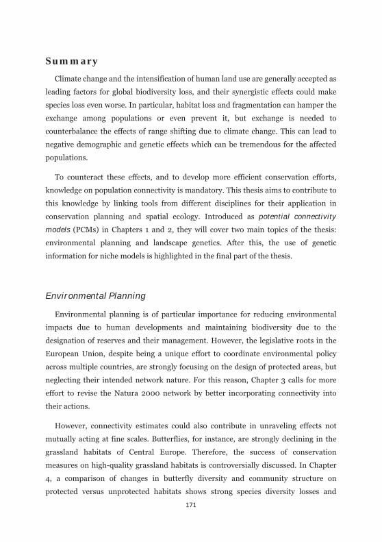
171
Summary
Climate change and the intensification of human land use are generally accepted as
leading factors for global biodiversity loss, and their synergistic effects could make
species loss even worse. In particular, habitat loss and fragmentation can hamper the
exchange among populations or even prevent it, but exchange is needed to
counterbalance the effects of range shifting due to climate change. This can lead to
negative demographic and genetic effects which can be tremendous for the affected
populations.
To counteract these effects, and to develop more efficient conservation efforts,
knowledge on population connectivity is mandatory. This thesis aims to contribute to
this knowledge by linking tools from different disciplines for their application in
conservation planning and spatial ecology. Introduced as potential connectivity
models (PCMs) in Chapters 1 and 2, they will cover two main topics of the thesis:
environmental planning and landscape genetics. After this, the use of genetic
information for niche models is highlighted in the final part of the thesis.
Environmental Planning
Environmental planning is of particular importance for reducing environmental
impacts due to human developments and maintaining biodiversity due to the
designation of reserves and their management. However, the legislative roots in the
European Union, despite being a unique effort to coordinate environmental policy
across multiple countries, are strongly focusing on the design of protected areas, but
neglecting their intended network nature. For this reason, Chapter 3 calls for more
effort to revise the Natura 2000 network by better incorporating connectivity into
their actions.
However, connectivity estimates could also contribute in unraveling effects not
mutually acting at fine scales. Butterflies, for instance, are strongly declining in the
grassland habitats of Central Europe. Therefore, the success of conservation
measures on high-quality grassland habitats is controversially discussed. In Chapter
4, a comparison of changes in butterfly diversity and community structure on
protected versus unprotected habitats shows strong species diversity losses and
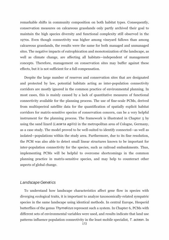
172
remarkable shifts in community composition on both habitat types. Consequently,
conservation measures on calcareous grasslands only partly archived their goal to
maintain the high species diversity and functional complexity still observed in the
1970s. Even though connectivity was higher among vineyard fallows than among
calcareous grasslands, the results were the same for both managed and unmanaged
sites. The negative impacts of eutrophication and monotonization of the landscape, as
well as climate change, are affecting all habitats—independent of management
concepts. Therefore, management on conservation sites may buffer against these
effects, but it is not sufficient for a full compensation.
Despite the large number of reserves and conservation sites that are designated
and protected by law, potential habitats acting as inter-population connectivity
corridors are mostly ignored in the common practice of environmental planning. In
most cases, this is mainly caused by a lack of quantitative measures of functional
connectivity available for the planning process. The use of fine-scale PCMs, derived
from multispectral satellite data for the quantification of spatially explicit habitat
corridors for matrix-sensitive species of conservation concern, can be a very helpful
instrument for the planning process. The framework is illustrated in Chapter 5 by
using the sand lizard (Lacerta agilis) in the metropolitan area of Cologne, Germany,
as a case study. The model proved to be well-suited to identify connected—as well as
isolated—populations within the study area. Furthermore, due to its fine resolution,
the PCM was also able to detect small linear structures known to be important for
inter-population connectivity for the species, such as railroad embankments. Thus,
implementing PCMs will be helpful to overcome shortcomings in the common
planning practice in matrix-sensitive species, and may help to counteract other
aspects of global change.
Landscape Genetics
To understand how landscape characteristics affect gene flow in species with
diverging ecological traits, it is important to analyze taxonomically-related sympatric
species in the same landscape using identical methods. In central Europe, Hesperid
butterflies of the genus Thymelicus represent such a system. In Chapter 6, PCMs with
different sets of environmental variables were used, and results indicate that land use
patterns influence population connectivity in the least mobile specialist, T. acteon. In
173
contrast, populations of the highly mobile generalist, T. lineola, were panmictic,
lacking any landscape-related effect on the weak genetic differentiation detected. In
the species with ecological traits in between those of the congeners, T. sylvestris,
climate had a strong impact on inter-population connectivity. The results show that
closely related species representing a gradient of ecological traits also show genetic
structures and landscape genetic relationships that gradually change from a
geographical macro- to micro-scale. Thus, the type and magnitude of landscape
effects on gene flow can strongly differ—even among closely-related species
inhabiting the same landscape—and depend on their relative degree of specialization.
In addition, the use of different genetic differentiation metrics makes it possible to
detect recent changes in the relative importance of landscape factors affecting gene
flow, which likely change as a result of contemporary habitat alterations.
Beside general patterns it is important to look also at local genetic effects. Because
landscapes are dynamic entities, where processes are locally affected in manifold
ways, genetic exchange is also likely to be affected by different locally-acting
landscape elements, generating spatial nonstationarity in gene flow estimates as a
result. Accounting for this source of uncertainty will enhance our understanding on
how the landscape affects genetic exchange and which key landscape elements are
driving it. Chapter 7 of this thesis proposes a method based on statistical learning
theory that optimizes the relationship between genetic distances by combining the
resistance surfaces of certain landscape elements. Using one of the above-mentioned
Hesperid butterflies and the wolverine (Gulo gulo) as examples, this approach was
introduced. The examples and literature review showed that this method would be
valuable for landscape genetics, and should be applicable to any method that
correlates genetic distances to a set of effective distances characterizing the
landscape.
Genes to the niche!
The final part of the thesis deals with the implication genetic information can have
on the conceptional roots of species distribution models (SDMs) also known as
environmental niche models (ENMs). The technological revolution in the past 25
years now allows the analysis of species occurrence information in completely novel
ways. ENMs appeared as a central tool in this regard, and they are frequently used to
174
address questions related to global change. Despite their popularity, ENMs often
suffer from a lack of biological realism and other methodological challenges. To this
end, researchers have begun to integrate genetic information into ENMs. However,
there is currently no conceptual framework that integrates population genetic
information into the theoretical assumptions made for ENMs. Chapter 8 highlights
five major reasons why the conceptual integration of genetic information in ENMs
can improve model predictions and refine underlying theory. Specifically, genetic
data can elucidate how environmental change alters functional connectivity, spatial
genetic structure, hybridization, density-dependent priority effects, and source-sink
dynamics. Thus, linking genetic and distribution data can lead to a better
understanding why species respond to environmental change in a certain way, and
improve our ability to forecast these responses. The chapter discusses these points in
the context of modeling challenges in the era of the Anthropocene, where habitat
fragmentation, biotic invasions, and climate change are major human-driven threads
to global biodiversity. That overview shows that integrating different kind of genetic
information into ENMs permits a more holistic view of niche theory and points to
shortcomings associated with how niche theory is currently being implemented in
ENMs.
175
Zusammenfassung
Klimawandel und eine stetig intensivere Landnutzung durch den Menschen sind
allgemeinhin als treibende Faktoren hinter dem globalen Biodiversitätsverlust
anerkannt. Betrachtet man beide Faktoren gemeinsam ist anzunehmen, dass sich
dieser Verlust in Zukunft weiter verstärkt und damit sämtliche Befürchtungen
übertrifft. Vor allem Habitatverlust und –fragmentierung sind sehr problematisch, da
hierdurch der Austausch von Individuen zwischen Populationen gebremst oder gar
komplett unterbunden wird. Dieser Austausch ist jedoch notwendig um die negativen
Effekte des Klimawandels zu kompensieren, etwa indem sich Artareale verschieben
könnten. Dies kann ungeheure negative Effekte auf demographische oder genetische
Eigenschaften von betroffenen Populationen haben.
Um diesen Effekten entgegenzuwirken, und damit effektivere Schutzbemühungen
zu entwickeln, ist Wissen zur Konnektivität von Populationen unerlässlich. Diese
Dissertation soll einen Beitrag zu diesem Wissen leisten, indem Methoden
verschiedener Fachdisziplinen zusammengeführt werden, um diese für die
Umweltplanung und der Raumökologie anwendbar zu machen. Dieses in den
Kapiteln 1 und 2 als „potentitelles Konnektivitätsmodell“ (PKM) eingeführte System
soll in zwei wesentlichen Themenbereichen Anwendung finden: Umweltplanung und
Landschaftsgenetik. Darüber hinaus soll in einem abschließenden dritten Teil der
Nutzen genetischer Informationen für prädiktive Nischenmodelle hervorgehoben
werden.
Umweltplanung
Umweltplanung ist von entscheidender Wichtigkeit, um negative Einflüsse von
Bauvorhaben auf Tiere und Pflanzen sowie auf deren Habitate zu bewerten und
gegebenenfalls zu kompensieren. Desweiteren soll erreicht werden Biodiversität als
Ganzes durch die Ausweisung von Schutzgebieten und deren Management zu
schützen. Die Europäische Union hat mit der FFH und der Vogelschutz-Richtlinie
(Natura 2000) ein beispielloses staatenübergreifendes rechtliches Rahmenwerk für
den Naturschutz geschaffen. Allerdings forcieren diese Richtlinien stark auf die
Ausweisung von Schutzgebieten anstatt auch auf eine entsprechende räumliche

176
Vernetzung dieser Gebiete verbindlich einzugehen. Kapitel 3 stellt diesen Missstand
in einem Kommentar auf eine entsprechende Facharbeit dar, die eine Vision für ein
Natura 2020 aufstellt, hierbei jedoch den mangelhaften Bezug zur Konnektivität
nicht andiskutiert.
Eine Quantifizierung von Konnektivität ist ebenfalls wichtig um Effekte auf lokaler
Ebene von solchen auf größeren Skalenebenen zu unterscheiden. Beispielsweise sind
viele Schmetterlingsarten in Offenlandlebensräumen in Mitteleuropa stark
rückläufig. Der Erfolg von Schutzbemühungen wird daher kontrovers diskutiert.
Kapitel 4 vergleicht Änderungen von Tagfalterzönosen in geschützten und
ungeschützten Offenlandlebensräumen von 1970 bis heute. Wenngleich die
Konnektivität höher zwischen ungeschützten Lebensräumen war sind die Ergebnisse
sehr ähnlich bei allen Standorten: Tagfalterzönosen änderten sich von artenreichen
zu artenärmeren und Generalist-dominierten Gesellschaften. Die negativen Effekte
von Eutrophierung und Monotonisierung der Landschaft, sowie des Klimawandels
beeinflussen sämtliche Habitate – ganz gleich wie deren Schutzbemühungen und
Managementkonzepte aussehen. Daher ist es möglich mit einem Management
geschützter Flächen (wie etwa einer extensiven Beweidung) großskalige Effekte
abpuffern, jedoch lassen sich diese damit nicht Kompensieren.
Trotz der großen Zahl an Schutzgebieten und Bemühungen für deren Ausweisung,
werden potentielle Vernetzungsstrukturen oftmals ignoriert in der Planungspraxis.
Meistens ist dies darauf zurückzuführen, dass die Möglichkeiten solche Strukturen
effektiv im Planungsprozess zu erfassen stark begrenzt sind. Feinskalige PKMs, die
auf multispektralen Fernerkundungsdaten beruhen können einen hilfreichen Ansatz
für die Umweltplanung darstellen, indem sie artrelevante Vernetzungsstrukturen
räumlich explizit für strukturgebundene Arten abbilden können. Dieses Konzept wird
in Kapitel 5 beispielhaft für die Zauneidechse (Lacerta agilis, L.) im Stadtgebiet von
Köln vorgestellt. Das Modell zeigt sehr gut räumliche Vernetzungsstrukuren, wie
beispielsweise Bahndämme an und bildet ebenfalls Habitate ab, in denen sich
Populationen aufhalten. Diese Populationen können nun klar als gut vernetzt oder
isoliert angesprochen werden. Durch die Implementierung von PKMs in der
Planungspraxis lassen sich somit einige Unzulänglichkeiten in der Bewertung von
strukturgebundenen Arten in Bezug auf die Vernetzung von Vorkommen sowie der
Definition von lokalen Populationen beheben.
177
Landschaftsgenetik
Um zu verstehen, wie Landschaftselemente Genfluss von Arten mit
unterschiedlichen ökologischen Eigenschaften beeinflussen ist es wichtig nah
verwandte Arten in den gleichen Studienräumen vergleichend zu untersuchen. In
Mitteleuropa stellen Dickkopffalter der Gattung Thymelicus ein solches System dar.
Kapitel 6 untersucht mithilfe von PKMs welche Rolle verschiedene
Landschaftselemente beim genetischen Austausch bei drei dieser Arten spielen. In
der am wenigsten mobilen jedoch am stärksten spezialisierten Art T. acteon zeigte
sich, dass Landnutzung ein wesentlicher Faktor für die genetische Vernetzung
darstellt. Demgegenüber zeigte sich beim mobilen Generalisten T. lineola eine
panmiktische genetische Struktur und somit keinerlei Korrelation mit irgendeinem
der untersuchten Landschaftselemente. Bei der dritten Art, T. sylvestris, welche
ökologisch zwischen seinen beiden Schwesternarten steht zeigte sich eine
ausgeprägte zunehmende genetische Isolation mit der geographischen Distanz. Diese
Korrelation bestand auch bei sämtlichen untersuchten Landschaftselementen.
Weitaus am stärksten war diese jedoch mit den klimatischen Eigenschaften des
Untersuchungsgebietes korreliert. Grundlegend deuten die Ergebnisse darauf hin,
dass Arten mit graduell unterschiedlichen ökologischen Eigenschaften sich ebenfalls
in ihren genetischen Antworten graduell unterscheiden. So in etwa mit der Skala, auf
der die unterschiedlichen Landschaftselemente wirken. Während Landnutzung eher
kleinräumig wirkt sind klimatische Charakteristika eher großräumig wirksam.
Darüber hinaus beleuchtet das Kapitel die Bedeutung von der Verwendung
unterschiedlicher genetischer Kennwerte bei solchen vergleichen, da mögliche
Inkonsistenzen auf sich ändernde ökologische Gleichgewichte infolge menschlicher
Eingriffe hinweisen können.
Neben solchen generellen Erkenntnissen ist es wichtig auch auf lokale Effekte zu
achten. Landschaften sind dynamisch und damit räumlich sehr heterogen. Prozesse
werden daher lokal in vielfältiger Weise beeinflusst. Genfluss als einer dieser
Prozesse macht hierbei keine Ausnahme und kann durch lokale
Landschaftscharakteristika unterschiedlich stark beeinflusst werden, die durch eine
ganzheitliche Betrachtung, gemittelt über eine Untersuchungsregion, unter
Umständen an Aussagekraft verlieren könnten. Dies führt letztlich zu räumlicher

178
Nonstationarität wodurch die nicht erklärte Varianz in einer Korrelation zwischen
genetischer Distanz und der effektiven Distanz einzelner betrachteter Faktoren
zunimmt. Diese potentielle Fehlerquelle zu berücksichtigen würde unser Verständnis
darüber erweitern, wie die Landschaft als Ganzes genetischen Austausch beeinflusst
und welche Landschaftselemente lokal dafür verantwortlich sind. Kapitel 7 der
Dissertation stellt eine Methode vor die auf den Prinzipien des statistischen Lernens
beruht und welche den Zusammenhang zwischen der Landschaft und des Genflusses
optimiert. Hierdurch werden Werte von Widerstandslandschaften unterschiedlicher
Landschaftselemente kombiniert und in eine einzige abhängige Variable überführt
und iterativ optimiert bis die Varianz des Zusammenhangs minimiert wurde. Diese
Methode wird im Kapitel 7 an zwei Fallbeispielen exemplarisch vorgestellt. Die
Beispiele und ein Literaturvergleich zeigen, dass die Logik der Methode eine
Bereicherung für landschaftsgenetische Untersuchungen hat und einfach für
verschiedene Verfahren modifiziert werden könnte, welche genetische Distanzen mit
effektiven Distanzen aus der Landschaft korrelieren.
Gene zu den Nischen!
Der letzte Teil der Doktorarbeit beschäftigt sich mit den Auswirkungen, die
genetische Informationen auf die konzeptionellen Grundlagen von prädiktiven
Nischenmodellen (SDMs & ENMs) haben können. Die technologische Revolution der
vergangenen 25 Jahre ermöglicht nun völlig neue Wege zur Untersuchung von
Arealsystemen. SDMs stellen hierbei ein zentrales Werkzeug dar, da diese häufig
genutzt werden um Fragen zum Globalen Wandel zu beantworten. Trotz ihrer
Popularität, fehlt es diesen Modellen, neben anderen methodischen
Herausforderungen, oft an biologischer Relevanz. Um diesem Problem zu begegnen
kombinieren Wissenschaftler nun SDMs vereinzelnd mit genetischen Informationen.
Allerdings existiert bislang kein konzeptionelles Rahmenwerk, welches
populationsgenetische Aspekte in die theoretischen Grundlagen von SDMs integriert.
Kapitel 8 zeigt fünf Gründe, wieso eine konzeptionelle Integration von genetischer
Information in SDMs sinnvoll ist, Modellvorhersagen verbessert und die den
Modellen zugrundeliegende Theorie erweitert. Im Speziellen könnten genetische
Daten zeigen, wie Veränderungen in der Umwelt auf funktionale Konnektivität,
räumliche genetische Struktur, Hybridisierung, dichteabhängige Effekte sowie auf

179
Source-Sink Dynamiken wirken. Somit könnte diese Integration zu einem besseren
Verständnis beitragen, wieso Arten auf bestimmte Änderungen reagieren wie sie es
tun und verbessern die Möglichkeiten zur Vorhersage dieser Reaktionen. Dieses
Kapitel illustriert diese Synthese mit Anthropozänen Beispielen, wo
Habitatfragmentierung, biologische Invasionen, und der Klimawandel große
Gefahren für die weltweite Biodiversität darstellen.

180

181
ACKNOWLEDGEMENTS
“Everyone you will ever meet knows something you don’t”
BILL NYE

182

183
Acknowledgements
Along the journey over the past three years that has been my dissertation, I came
across many people that I would like to thank.
First, I would like to thank my supervisors, Wolfgang J. Wägele and Bernhard
Misof, for always being supportive and giving me all the freedom I needed to develop
my ideas and turn them into research. I also want to thank Niko Balkenhol for
guiding me through my first steps into landscape genetics, and Dennis Rödder for his
long-lasting support and giving me the passion for SDMs, which formed a solid basis
for my dissertation and my academic career as a whole; it has been a pleasure for me
to have crossed your paths and learn from you both!
I also want to thank my main funding bodies, the German Federal Environmental
Foundation (DBU) for funding me over the past three years, and the German
Academic Exchange Service (DAAD) for supporting my three-month research stay in
the US. In particular, I want to thank Volker Wachendörfer at DBU for always being
supportive and for organizing the nice fellowship retreats from which I learned so
much and met many new people. In addition, I want to thank the DAAD, the German
Ornithological Society (DO-G), the Swiss Society for the Study and Conservation of
Birds (ALA) and the Alexander Koenig Gesellschaft (AKG) for funding various trips to
conferences that would have been impossible to finance on my own. Thanks to you, I
could present my work, expand my professional network and explore new places on
earth, widening my horizon for not only nature, but also humanity.
My very special thanks go to all my collaborators that came across my way during
the past years, and without which this thesis would have been impossible in its
current form. Namely, I want to thank Katharina J. Filz and Thomas Schmitt for our
mutual cooperation on butterflies during Katharina’s PhD, which I could use for
developing my ideas on connectivity that ended up as a collaborative work in Chapter
4. Staying with butterflies, I would like to thank Jan C. Habel for his permanent
support and collaboration from which I learned so much. Your openness to
collaborate and your attitude on science—with all its good and bad points—have
deeply inspired me and made up an important part of my professional self. I also
want to thank Anna F. Cord and Johannes Stoffels for their input on Remote
Sensing—a field that was entirely new to me, but has gained my attraction during my

184
thesis and definitely will remain a crucial aspect in my future work. In addition, I also
want to express my gratitude to Petra Dieker, Christoph Ring, Ursula Bott, Michelle
Bußler, Joseph D. Chipperfield, Martin Husemann, Deborah A. Dawson, Alain
Frantz, Johannes Signer, Hendrik “Henne” Edelhoff and Femke Pflüger for their
help, feedback, fruitful discussions, and/or data preparation at different stages of the
thesis. In particular, I want to thank Sven Nekum for his outstanding efforts in
sampling sand lizard records during his Diploma thesis, which formed the basis for
introducing PCMs for environmental planning in Chapter 5. And not forgetting
Veronica Frans, thank you for all the proofreading you did and the great collaboration
so far!
My stay abroad—despite it having been for only three months—really gave me a
boost during the final year of my dissertation; it was a golden opportunity to step into
a different academic system with one of the world’s leading biogeographers and
experts in SDMs and niche theory. Therefore, my thanks go to Catherine H. Graham
for being willing to have me and offering some of the best moments during my
academic career so far. You have been an inspiring example since my first steps into
SDMs, where one is inevitably stumbling across your work. It was a great pleasure for
me to receive your input and feedback during that time and the times thereafter! It
was also Catherine’s lab and the whole department that made my time spent so
worthwhile. To this end, I want to thank Anusha Shankar, Marisa Lim, Guillermo
Fandoz, Brunno Oliveira, Ben Weinstein, Laura Gambino, Emily Runnels, Michael
Schrimpf and Maureen Lynch for a memorable three months at campus, during
birding, and many social events. Further, I want to thank Jonathan Greenfield and
his lovely family which have been my social heart outside of academic life during my
stay in New York. Thank you, Jonathan, for replying to my request to couchsurf and
offering me way more than a couch and what I’ve ever dreamed of: a great host
family.
Staying with family, I want to thank my mother, Solveigh Weber, for her
permanent and continuing support, and for exploring nature together during my
childhood, which founded the roots for my passion for ecology and science in general.
Vielen Dank, dass du mir die Natur von kleinauf nah gebracht und meinen
Wissensdurst gestillt hast und ich hieraus meine Begeisterung für die Natur und die
Wissenschaft überhaupt erst entwickeln konnte!

185
Last but not least, I want to thank my partner, Stefanie Bußler, for her love and
patience during my thesis. Achieving a proper work-life balance would have been
impossible without you. You are the “life” part of this equation, from which I receive
my motivation for the “work” part of it. I love you!

186
187
References
ABRAMS M 2000: The Advanced Spaceborn Thermal Emission and Reflection
Radiometer (ASTER): data products for the high spatial resolution imager on
NASA's Terra platform. Int J Remote Sens 21: 847–859.
ADDISON PFE, RUMPFF L, BAU SS, CAREY JM, CHEE YE, JARRAD FC, MCBRIDE MF,
BURGMAN MA 2013: Practical solutions for making models indispensable in
conservation decision-making. Div Distr 19:490–502.
ADRIAENSEN F, CHARDON JP, DE BLUST G, SWINNEN E, VILLALBA S, GULINCK H,
MATTHYSEN E 2003: The application of ‘least cost’ modelling as a functional
landscape model. Landsc Urban Plan 64: 233–247.
AGASYAN A, AVCI A, TUNIYEV B, LYMBERAKIS P, ANDRÉN C, COGALNICEANU D, WILKINSON
J, ANANJEVA N, ÜZÜM N, ORLOV N, PODLOUCKY R, TUNIYEV S, KAYA U, CRNOBRNJA
ISAILOVIC J, VOGRIN M, CORTI C, PÉREZ MELLADO V, SÁ-SOUSA P, CHEYLAN M,
PLEGUEZUELOS J, KYEK M, WESTERSTRÖM A, NETTMANN HK, BORCZYK B,
STERIJOVSKI B, SCHMIDT B 2010: Lacerta agilis, in: IUCN 2012. IUCN Red List of
Threatened Species. Version 2012.2. Accessed via: www.iucnredlist.org.
AITKEN M 1996: A general maximum likelihood analysis of overdispersion in
generalized linear models. Stat Comp 6: 251–262.
ALVARADO-SERRANO DF & KNOWLES LL 2014: Ecological niche models in
phylogeographic studies: applications, advances and precautions. Mol Ecol Res
14: 233–248.
AMSELLEM L, NOYER JL, LE BOURGEOIS T, HOSSAERT-MCKEY M 2000: Comparison of
genetic diversity of the invasive weed Rubus alceifolius Pior. (Rosaceae) in its
native range and in areas of introduction, using amplified fragment length
polymorphism (AFLP) markers. Mol Ecol 9: 443–455.
ANDERSEN LW, FOG K, DAMGAARD C 2004: Habitat fragmentation causes bottlenecks
and inbreeding in the European tree frog (Hyla arborea). Proc R Soc B 271:1293–
1302.
ANDERSON NJ, BUGMANN H, DEARING JA, GAILLARD M-J 2006: Linking
palaeoenvironmental data and models to understand the past and predict the
future. TREE 21: 696–704.
188
ANDRÉN H 1994: Effects on habitat fragmentation on birds and mammals in
landscapes with different proportions of suitable habitat: a review. Oikos 71:355–
366.
ANGETTER LS, LÖTTERS S, RÖDDER D 2011: Climate niche shift in invasive species: the
case of the brown anole. Biol J Linn Soc 104: 943–954.
ARAI K, TONOOKA H 2005: Radiometric performance evaluation of ASTER VNIR,
SWIR and TIR. IEEE Trans Geosci Remote Sens 43: 2725–2732
ARAÚJO MB, CABEZA M, THULLIER W, HANNAH L, WILLIAMS PH 2004: Would climate
change drive species out of reserves? An assessment of existing reserve-selection
methods. Glob Change Biol 10: 1618–1626.
ARAÚJO MB, PEARSON RG, THUILLER W, ERHARD M 2005: Validation of species-
climate impact models under climate change. Glob Change Biol 11: 1504–1513.
ARNOLD ML 1997: Natural hybridization and evolution, Oxford.
AUBRY KB, MCKELVEY KS, COPELAND JP 2007: Distribution and broadscale habitat
relations of the wolverine in the contiguous United States. J Wildl Manag 71:
2147–2158.
BAGUETTE M, STEVENS VM, CLOBERT J 2014: The pros and cons of applying the
movement ecology paradigm for studying animal dispersal. Movement Ecol 2:13.
BALDWIN RA 2009: Use of maximum entropy modeling in wildlife research. Entropy
11: 854–866.
BALKENHOL N, WAITS LP, DEZZANI RJ 2009: Statistical approaches in landscape
genetics: an evaluation of methods for linking landscape and genetic data.
Ecography 32: 818–830.
BALKENHOL N, PARDINI R, CORNELIUS C, FERNANDES F, SOMMER S 2013: Landscape-
level comparison of genetic diversity and differentiation in a small mammal
inhabiting different fragmented landscapes of the Brazilian Atlantic Forest.
Conserv Gen 14: 355–367.
BALKENHOL N, CUSHMAN SA, WAITS LP, STORFER A 2015a: Current status, future
opportunities, and remaining challenges in landscape genetics. In: BALKENHOL N,
CUSHMAN SA, STORFER AT, WAITS LP (eds): Landscape Genetics: concepts,
methods, applications. Wiley.
189
BALKENHOL N, CUSHMAN SA, STORFER A, WAITS LP 2015b: Introduction to landscape
genetics – concepts, methods, applications. In: BALKENHOL N, CUSHMAN SA,
STORFER AT, WAITS LP (eds): Landscape Genetics: concepts, methods,
applications. Wiley.
BALMER E, ERHARDT A 2000: Consequences of succession on extensively grazed
grasslands for central European butterflies: Rethinking Conservation practices.
Conserv Biol 14: 746–757.
BARTHOLMESS H, SCHLOTTMANN K, NOBEL W 2011: Immission measurements with
diffusive samplers and lichen mappings to show the impact of nitrogen in the
environment and its effects. Gefahrstoffe Reinhaltung der Luft 71: 165–172.
BEAUMONT LJ, HUGHES L, POULSEN M 2005: Predicting species distributions: use of
climatic parameters in BIOCLIM and its impact on predictions of species’ current
and future distributions. Ecol Mod 186: 250–269.
BELL RC, PARRA JL, TONIONE M, HOSKIN CJ, MACKENZIE JB, WILLIAMS SE, MORITZ C
2010: Patterns of persistence and isolation indicate resilience to climate change in
montane rainforest lizards. Mol Ecol 19: 2531–2544.
BELLARD C, BERTELSMEIER C, LEADLEY P, THUILLER W, COURCHAMP F 2012: Impacts of
climate change on the future of biodiversity. Ecol Lett 15:365–377.
BENES J, KURAS T 1998: Long term diversity changes of butterflies and burnets of the
Opavska pahorkatina Hills and Nizky Jesenik Mts. (Czech Republic). Casopis
Slezskeho Muzea Opava 47: 245–270.
BENNETT AF, CROOKS KR, SANJAYAN M 2006: The future of connectivity conservation.
In: Connectivity conservation (ed. CROOKS KR, SANJAYAN M). Cambridge
University Press, Cambridge, pp. 676–694.
BERGLIND S-A 2000: Demography and management of relict Sand Lizard Lacerta
agilis populations on the edge of extinction. Ecol Bull 48:123–142.
BERGLIND S-A 2004: Sand Lizard (Lacerta agilis) in central Sweden – modeling
juvenile reintroduction and spatial management strategies for metapopulation
establishment. In: AKCAKAYA HR et al. (eds) Species conservation and
management: case studies. Oxford University Press.
BIELEFELD U 1985: Aufbau eines vernetzten Biotopsystems, Trocken- und
Halbtrockenrasen in Rheinland-Pfalz. Ministerium für Soziales, Gesundheit und
190
Umwelt. Arten- und Biotopschutz - Aufbau eines vernetzten Biotopsystems.
Ergebnis der Fachtagung 1984. Verlag Sommer, Lahnstein.
BINK FA 1992: Ecologische Atlas van de Dagvlinders van Noordwest-Europa. Schuyt
& Co. Uitgevers en Importeurs, Haarlem.
BIVAND RS, PEBESMA E, GOMEZ-RUBIO V 2013: Applied spatial data analysis with R,
Second edition. Springer.
BLANKE I 1999: Erfassung und Lebensweise der Zauneidechse (Lacerta agilis) an
Bahnanlagen. Zeitschrift für Feldherpetologie 6:147–159.
BLANKE I (2010) Die Zauneidechse - Zwischen Licht und Schatten. Laurenti, Bielefeld,
Germany.
BOLLIGER J, LANDER T, BALKENHOL N 2014: Landscape genetic since 2003: status,
challenges and future directions. Landsc Ecol 29: 361–366.
BOTERO CA, WEISSING FJ, WRIGHT J, RUBENSTEIN DR 2015: Evolutionary tipping
points in the capacity to adapt to environmental change. PNAS 112: 184–189.
BOURN NAD, THOMAS JA 2002: The challenge of conserving grassland insects at the
margins of their range in Europe. Biol Conserv 104: 285–292.
BRAMBILLA M, FICETOLA GF 2012: Species distribution models as a tool to estimate
reproductive parameters: a case study with a passerine bird species. J Anim Ecol
81: 781–787.
BRAUNISCH V, SEGELBACHER G, HIRZEL AH 2010: Modelling functional landscape
connectivity from genetic population structure: a new spatially explicit approach.
Molecular Ecology 19: 3664–3678.
BRAUNISCH V, COPPES J, ARLETTAZ R, SUCHANT R, SCHMID H, BOLLMANN K 2013:
Selecting from correlated climate variables: a major source of uncertainty for
predicting species distributions under climate change. Ecography 36: 971–983.
BROUAT C, CHEVALLIER H, MEUSNIER S, NOBLECOURT T, RASPLUS J-Y 2004:
Specialization and habitat: spatial and environmental effects on abundance and
genetic diversity of forest generalist and specialist Carabus species. Mol Ecol 13:
1815–1826.
191
BRUNSDON C, FOTHERINGHAM AS, CHARLTON ME 1996: Geographically weighted
regression: a method for exploring spatial nonstationarity. Geogr Analysis 28:
281–298.
BURGGRAAFF P, KLEEFELD KD 1998: Historische Kulturlandschaft und
Kulturlandschaftselemente: Ergebnisse aus dem F+E-Vorhaben 808 09 075 des
Bundesamtes für Naturschutz. BfN-Schr.-Vertrieb im Landwirtschaftsverl,
Münster.
BURNHAM KP, ANDERSON DR 2002: Model selection and multimodel inference: a
practical information-theoretic approach. New York: Springer.
BURROUGH PA, MCDONNELL R 1998: Principles of geographical information systems.
Oxford University Press, Oxford.
BUTCHART SHM, WALPOLE M, COLLEN B, VAN STRIEN A, SCHARLEMANN JPW, ALMOND
REA, BAILLIE JEM, BOMHARD B, BROWN C, BRUNO J, CARPENTER KE, CARR GM,
CHANSON J, CHENERY AM, CSIRKE J, DAVIDSON NC, DENTENER F, FOSTER M, GALLI A,
GALLOWAY JN, GENOVESI P, GREGORY RD, HOCKINGS M, KAPOS V, LAMARQUE J-F,
LEVERINGTON F, LOH J, MCGEOCH MA, MCRAE L, MINASYAN A, MORCILLO MH,
OLDFIELD TEE, PAULY D, QUADER S, REVENGA C, SAUER JR, SKOLNIK B, SPEAR D,
STANWELL-SMITH D, STUART SN, SYMES A, TIERNEY M, TYRRELL TD, VIÉ J-C,
WATSON R 2010: Global biodiversity: Indicators of recent declines. Science, 328:
1164–1168.
CABRAL JS, KREFT H 2012: Linking ecological niche, community ecology and
biogeography: insights from a mechanistic niche model. J Biogeogr 39: 2212–
2224.
CALDWELL LK 1991: Analysis – assessment – decision: the anatomy of rational
policymaking. Impact Assessment Bulletin 9:81–92.
CANTER L, ROSS B 2010: State of practice of cumulative effects assessment and
management: the good, the bad and the ugly. Impact Assessment and Project
Appraisal 28:261–268.
CARNAVAL AC, MORITZ C 2008: Historical climate modelling predicts patterns of
current biodiversity in the Brazilian Atlantic forest. J Biogeogr 25: 1187–1201.
CASETTI E 1972: Generating models by the expansion method: applications to
geographic research. Geogr Analysis 4: 81–91.
192
CHAN LM, BROWN JL, YODER AD 2011: Integrating statistical genetic and geospatial
methods bring new power to phylogeography. Molecular Phylogenetics and
Evolution 59: 523–537.
CHANDRA AK, RAGHAVAN R, RUZZO WL, SMOLENSKY R, TIWARI P 1997: The electrical
resistance of a graph captures its commute and cover times. Comp complex 6:
312–340.
CHEN G, ZHAO K, MCDERMID GJ, HAY GJ 2012: The influence of sampling density on
geographically weighted regression: a case study using forest canopy height and
optical data. Int J Rem Sen 33: 2909–2924.
CONRADT L, ROPER TJ, THOMAS CD 2001: Dispersal behaviour of individuals in
metapopulations of two British butterflies. Oikos 95: 416–424.
COPELAND JP, MCKELVEY KS, AUBRY KB, LANDA A, PERSSON J, INMAN RM, KREBS J,
LOFROTH E, GOLDEN H, SQUIRES JR, MAGOUN A, SCHWARTZ MK, WILMOT J,
COPELAND CL, YATES RE, KOJOLA I, MAY R 2010: The bioclimatic envelope of the
wolverine: Do climatic constraints limit their geographic distribution? Canadian J
Zool 88: 233–246.
CORD AF, RÖDDER D 2011: Inclusion of habitat availability in species distribution
models through multi-temporal remote-sensing data? Ecol App 21: 3285–3298.
CORDELLIER M, PFENNINGER M 2009: Inferring the past to predict the future: climate
modeling predictions and phylogeography for the freshwater gastropod Radix
balthica (Pulmonata, Basommatophora). Mol Ecol 18: 534–544.
CORLETT RT 2014: The Anthropocene concept in ecology and conservation. TREE 30:
36–41.
COUNCIL OF THE EUROPEAN COMMISSION 1992: Council Directive 92/43/EEC of 21 May
1992 on the conservation of natural habitats and of wild fauna and flora. Official
Journal of the European Communities, Series L 206:7–49.
CRANDALL KA, BININDA-EMONDS ORP, MACE GM, WAYNE RK 2000: Considering
evolutionary processes in conservation biology. TREE 15: 290–295.
CRAWFORD NG 2009: SMOGD: software for the measurement of genetic diversity.
Mol Ecol Res 10: 556–557.
193
CRIST EP, CICONE RC 1984: Application of the Tasseled Cap Concept to Simulated
Thematic Mapper Data, Photogr Engin Rem Sen 50:343–352.
CROOKS KR, SANJAYAN M (2006) Connectivity conservation. Cambridge University
Press.
CUSHMAN SA, LANDGUTH RL 2010: Spurious correlations and inference in landscape
genetics. Mol Ecol 19: 3592–3602.
CUSHMAN SA, WASSERMANN TN, LANDGUTH EL, SHIRK AJ 2013: Re-evaluating causal
modeling with Mantel tests in landscape genetics. Diversity 5: 51–72.
DAWSON MN 2012: Parallel phylogeographic structure in ecologically similar
sympatric sister taxa. Mol Ecol 21: 987–1004.
DE SMEDT P 2010: The use of impact assessment tools to support sustainable policy
objectives in Europe. Ecol Soc 15:30.
DENNIS RLH, EALES H 1997: Patch occupancy in Coenonympha tullia (Müller 1764)
(Lepidoptera: Satyrinae): Habitat quality matters as much as patch size and
isolation. J Insect Conserv 1: 167–176.
DETWILER JT, CRISCIONE CD 2014: Recently introduced invasive geckos quickly reach
population genetic equilibrium dynamics. Biol Inv 16: 2653–2667.
DEVICTOR V, VAN SWAAY C, BRERETON T, BROTONS L, CHAMBERLAIN D, HELIÖLÄ J,
HERRANDO S, JULLIARD R, KUUSSAARI M, LINDSTRÖM Å, REIF J, ROY DB, SCHWEIGER
O, SETTELE J, STEFANESCU C, VAN STRIEN A, VAN TURNHOUT C, VERMOUZEK Z,
WALLISDE VRIES M, WYNHOFF I, JIGUET F 2012: Differences in the climatic debts of
birds and butterflies at a continental scale. Nature Clime Change 2:121–124.
DEVITT TJ, CAMERON DEVITT, SE, HOLLINGWORTH BD, MCGUIRE JA, MORITZ C 2013:
Montane refugia predict population genetic structure in the Large-blotched
Ensatina salamander. Mol Ecol 22: 1650–1665.
DEVKOTA ML, HATFIELD G, CHINTALA R 2014: Effect of sample size on the performance
of ordinary least squares and geographically weighted regression. Br J Math &
Comp Sci 4: 1–21.
DICKERSON W, MONTGOMERY J 1993: Substantive scientific and technical guidance for
NEPA analysis: pitfalls in the real world. The Environmental Professional 15:7–11.
194
DIETZ JM, GILADI I 2009: Scale-dependence of habitat sources and sinks. In: LIU J,
HULL V, MORZILLO AT, WIENS JA (eds): Sources, sinks and sustainability.
Cambridge University Press.
DINIZ-FILHO JAF, BINI LM 2012: Thirty-five years of spatial autocorrelation analysis
in population genetics: an essay in honour of Robert Sokal (1926-2012). Biol J
Linn Soc 107: 721–736.
DOERR VAJ, BARRETT T, DOERR ED 2011: Connectivity, dispersal behavior and
conservation under climate change: a response to Hogson et al. J Appl Ecol
48:143–147.
DORMANN CF, MCPHERSON JM, ARAÚJO MB, BIVAND R, BOLLIGER J, CARL G, DAVIES RG,
HIRZEL A, JETZ W, KISSLING WD, KÜHN I, OHLEMÜLLER R, PERES-NETO PR,
REINEKING B, SCHRÖDER B, SCHURR FM, WILSON R. 2007: Methods to account for
spatial autocorrelation in the analysis of species distributional data: a review.
Ecography 30: 609–628.
DORMANN CF, SCHYMANSKI SJ, CABRAL J, CHUINE I, GRAHAM C, HARTIG F, KEARNEY M,
MORIN X, RÖMERMANN C, SCHRÖDER B, SINGER A 2012: Correlation and process in
species distribution models: bridging a dichotomy. J Biogeogr 39: 2219–2131.
DORMANN CF, ELITH J, BACHER S, BUCHMANN C, CARL G, CARRÉ G, GARCÍA MARQUÉZ JR,
GRUBER B, LAFOURCADE B, LEITÃO PJ, MÜNKEMÜLLER T, MCCLEAN C, OSBORNE PE,
REINEKING B, SCHRÖDER B, SKIDMORE AK, ZURELL D, LAUTENBACH S 2013:
Collinearity: a review of methods to deal with it and a simulation study evaluating
their performance. Ecography 36:27–46.
DOVER J, SETTELE J 2009: The influences of landscape structure on butterfly
distribution and movement: a review. J Insect Conserv 13: 3–27.
DOYLE PG, SNELL JL 1984: Random walks and electric networks. Mathematical
Association of America.
DRIEZEN K, ADRIAESEN F, RONDININI C, DONCASTER CP, MATTHYSEN E 2007: Evaluating
least-cost model predictions with empirical dispersal data: a case-study using
radiotracking data of hedgehogs (Erinaceus europaeus). Ecol Mod 209:314–322.
DUDANIEC RY, SPEAR SF, RICHARDSON JS, STORFER A 2012: Current and historical
drivers of landscape genetic structure differ in core and peripheral salamander
populations. PLoS one 7: e36769.
195
DUFORET-FREBOURG N, BLUM MGB 2014: Nonstationarity patterns of isolation-by-
distance: inferring measures of local genetic differentiation with Bayesian kriging.
Evolution 68: 1110–1123.
DUINKER PN, BURBIDGE EL, BOARDLEY SR, GREIG LA 2013: Scientific dimensions of
cumulative effects assessment: toward improvements in guidance for practice.
Environ Rev 21: 40–52.
DYER RJ 2015a: Is there such a thing as landscape genetics? Mol Ecol 24: 3518–3528.
DYER RJ 2015b: Landscapes and plant population genetics. In: BALKENHOL N,
CUSHMAN S, STORFER A, WAITS L (eds). Landscape genetics: concepts, methods,
applications. Wiley.
EBERT G, RENNWALD E (eds) 1991: Die Schmetterlinge Baden-Württembergs, Band 1
und 2. Verlag Eugen Ulmer.
EEA. 2010: EEA Technical Report 12/2010, EU 2010 Biodiversity Baseline.
http://www.eea.europa.eu/publications/eu-2010-biodiversity-baseline/. (visited
Feb. 5, 2013)
ELITH J, GRAHAM CH, ANDERSON RP, DUDÍK M, FERRIER S, GUISAN A, HIJMANS RJ,
HUETTMANN F, LEATHWICK JR, LEHMANN A, LI J, LOHMANN LG, LOISELLE BA,
MANION G, MORITZ C, NAKAMURA M, NAKAZAWA Y, OVERTON JMCC, PETERSON AT,
PHILLIPS SJ, RICHARDSON KS, SCACHETTI PEREIRA R, SCHAPIRE RE, SOBERÓN J,
WILLIAMS S, WISZ MS, ZIMMERMANN NE 2006: Novel methods improve prediction
of species’ distributions from occurrence data. Ecography 29:129–151.
ELITH J, PHILLIPS SJ, HASTIE T, DUDÍK M, CHEE YE, YATES C 2011: A statistical
explanation of MaxEnt for ecologists. Div Distr 17: 43–47.
ELLIS JR, PASHLEY CH, BURKE JM, MCCAULEY DE 2006: High genetic diversity in a
rare and endangered sunflower as compared to a common congener. Mol Ecol 15:
2345–2355.
ELLWANGER G 2004: Lacerta agilis (Linnaeus, 1758), In: PETERSEN B, ELLWANGER G,
BLESS R, BOYE P, SCHRÖDER E, SSYMANK A (eds): Das europäische
Schutzgebietssystem Natura 2000 - Ökologie und Verbreitung von Arten der
FFH-Richtlinie in Deutschland - Band 2: Wirbeltiere. BfN, Bonn Bad-Godesberg,
pp 90–97.
196
ENGLER JO, RÖDDER D, ELLE O, HOCHKIRCH A, SECONDI J 2013: Species distribution
models contribute to determine the effect of climate and interspecific interactions
in moving hybrid zones. Journal of Evolutionary Biology 26: 2487–2496.
ENGLER JO, BALKENHOL N, FILZ KJ, HABEL JC, RÖDDER D 2014: Comparative
landscape genetics of three closely related sympatric Hesperid butterflies with
diverging ecological traits. PLoS one 9: e106526.
EU 1992: Council directive 92/43/EEC of 21 May 1992 on the conservation of natural
habitats and of wild fauna and flora. Official J., L206 (July), 7–50.
EXCOFFIER L, LARVAL G, SCHNEIDER S 2005: Arlequin ver. 3.0: an integrated software
package for population genetics data analysis. Evol Bioinform Onl 1: 47–50.
FAHRING L 2003: Effects of habitat fragmentation on biodiversity. Ann Rev Ecol Evol
Syst 34:487–515.
FAGAN WF, CALABRESE JM 2006: Quantifying connectivity: balancing metric
performance with data requirements. In: CROOKS KR, SANJAYAN M (eds)
Connectivity conservation. Cambridge University Press.
FELSENSTEIN J 1985: Confidence limits on phylogenies: An approach using the
bootstrap. Evolution, 39: 783–791.
FICETOLA GF, THUILLER W & MIAUD C 2007: Prediction and validation of the potential
global distribution of a problematic alien invasive species – the American bullfrog.
Div Distr 13: 476–485.
FICETOLA GF, MAIORANO L, FALCUCCI A, DENDONCKER N, BOITANI L, PADOA-SCHIOPPA E,
MIAUD C, THUILLER W 2010: Knowing the past to predict the future: land-use
change and the distribution of invasive bullfrogs. Glob Change Biol 16: 528–537.
FIELDING AH, BELL JF 1997: A review of methods for the assessment of prediction
errors in conservation presence/absence models. Env Cons 24: 38–49.
FILZ KJ, ENGLER JO, STOFFELS J, WEITZEL M, SCHMITT T 2013a: Missing the target? A
critical view on butterfly conservation efforts on calcareous grasslands. Biodiv
Conserv 22: 2223–2241.
FILZ KJ, SCHMITT T & ENGLER JO 2013b: How fine is fine-scale? Questioning the use of
fime-scale bioclimatic data in species distribution models to forecast abundance
patterns in butterflies. Eur J Enthomol 110: 311–317.
197
FINGER A, ZACHOS FE, SCHMITT T, MEYER M, ASSMANN T, HABEL JC 2008: The genetic
status of the Violet Copper Lycaena helle – a relict of the cold past in times of
global warming. Ecography 32: 382–390.
FITHIAN W, HASTIE T 2013: Finite-sample equivalence in statistical models for
presence-only data. Ann App Stat 7:1917–1939.
FISCHER J, LINDENMAYER DB 2007: Landscape modification and habitat
fragmentation: a synthesis. Glob Ecol Biogeogr 16:265–280.
FORDHAM D, BROOK B, MORITZ C, NOGUÉS-BRAVO D 2014: Better forecasts of range
dynamics using genetic data. TREE 29: 436–443.
FOSTER SA, GORR WL 1986: An adaptive filter for estimating spatially varying
parameters: application to modeling police hours spent in response to calls for
service. Manag Sci 32: 878–889.
FOTHERINGHAM AS, BRUNSDON C, CHARLTON ME 2002: Geographically weighted
regression: the analysis of spatially varying relationships. Wiley.
FOURCADE Y, ENGLER JO, RÖDDER D, SECONDI J 2014: Mapping species distribution
with MAXENT using a geographically biased sample of presence data: a
performance assessment of methods for correcting sampling bias. PLoS one 9:
e97122.
FRANKLIN J 2009: Mapping species distributions: Spatial inference and prediction.
Cambridge University Press, Cambridge.
FURRER RD, PASINELLI G 2015: Empirical evidence for source-sink populations: a
review on occurrence, assessments and implications. Biol Rev
doi:10.1111/brv.12195.
GAEDICKE R, HEINICKE W (eds.) 1999: Verzeichnis der Schmetterlinge Deutschlands
(Entomofauna Germanica 3). Entomologische Nachrichten und Berichte
(Dresden) 5: 1–216.
GAGGIOTTI OE 1996: Population genetic models of source sink metapopulations. T
Pop Biol 50: 178–208.
GAO BC 1995: Normalized Difference Water Index for Remote Sensing of Vegetation
Liquid Water from Space. Proceedings of SPIE 2480: 225–236.
198
GASTON KJ 2003: The structure and dynamics of geographic ranges. Oxford
University Press.
GAUDEUL M, GIRAUD T, KISS L, SHYKOFF JA 2011: Nuclear and Chloroplast
microsatellites show multiple introductions in the worldwide invasion history of
common ragweed, Ambrosia artemisiifolia. PLoS one 6:e17658.
GENELETTI D 2006: Some common shortcomings in the treatment of impacts of linear
infrastructures on natural habitat. EIA Rev 26:257–267.
GERLACH G, JUETERBOCK A, KRAEMER P, DEPPERMANN J, HARMAND P 2010:
Calculations of population differentiation based on GST and D: forget GST but not
all of statistics! Mol Ecol 19: 3845–3852.
GILBERT-NORTON L, WILSON R, STEVENS JR, BEARD KH 2010: A meta-analytic review
of corridor effectiveness. Conserv Biol 24: 660–668.
GITZENDANNER MA, SOLTIS PS 2000: Patterns of genetic variation in rare and
widespread plant congeners. Am J Bot 87: 783–792.
GLANDT D, BISCHOFF W 1988: Biology and conservation of the Sand Lizard (Lacerta
agilis). Mertensiella, 1:1–257
GOLDBERG CS, WAITS LP 2010: Comparative landscape genetics of two pond–breeding
amphibian species in a highly modified agricultural landscape. Mol Ecol 19:
3650–3663.
GOLDSTEIN H 1987: Multilevel models in educational and social research. Oxford
University Press.
GONTIER M 2006: Integrating landscape ecology in environmental impact assessment
using GIS and ecological modeling. In: TRESS B, TRESS G, FRY G, OPDAM P (eds)
From landscape research to landscape planning: aspects of integration, education
and application, Bakkaveen, The Netherlands, pp 345–354.
GONTIER M, MÖRTBERG U, BALFORS B 2010: Comparing GIS-based habitat models for
applications in EIA and SEA. EIA Rev 30:8–18.
GONZALEZ SC, SOTO-CENTENO JA, REED DL 2011: Population distribution models:
species distributions are better modelled using biologically relevant data
partitions. BMC Ecology 11: 20.
199
GOODWIN BJ 2003: Is landscape connectivity a dependent or independent variable?
Landscape Ecol 18: 687–699.
GOSLEE SC, URBAN DL 2007: The ecodist package for dissimilarity-based analysis of
ecological data. J Stat Softw 22: 1–19.
GOTELLI N, STANTON-GEDDES J 2015: Climate change, genetic markers and species
distribution modelling. J Biogeogr 42: 1577–1585.
GROOT AT, CLASSEN A, INGLIS O, BLANCO CA, LÓPEZ JR. J, TÉRAN VARGAS A, SCHAL C,
HECKEL DG, SCHÖFL G 2011: Genetic differentiation across North America in the
generalist moth Heliothis virescens and the specialist H. subflexa. Mol Ecol 20:
2676–2692.
GUILLERA-ARROITA G, LAHOZ-MONFORT JJ, ELITH J, GORDON A, KUJALA H, LENTINI PE,
MCCARTHY MA, TINGLEY R, WINTLE BA 2015: Is my species distribution model fit
for purpose? Matching data and models to applications. Glob Ecol Biogeogr, 24:
276—292.
GUILLOT G, SANTOS F 2009: A computer program to simulate multilocus genotype
data with spatially auto-correlated allele frequencies. Mol Ecol Res 9: 1112–1120.
GUILLOT G, MORTIER F, ESTOUP A 2005: Geneland: a program for landscape genetics.
Mol Ecol Notes 5: 712–715.
GUISAN A, ZIMMERMAN NE 2000: Predictive habitat distribution models in ecology.
Ecol Model 135: 147–186.
GUISAN A, THUILLER W 2005: Predicting species distributions: offering more than
simple habitat models. Ecol Lett 8: 993–1003.
GUISAN A, GRAHAM CH, ELITH J, HUETTMANN F 2007: Sensitivity of predictive species
distribution models to change in grain size. Div Dist 13: 332–340.
GUISAN A, TINGLEY R, BAUMGARTNER JB, NAUJOKAITIS-LEWIS I, SUTCLIFFE PR, TULLOCH
AI, REAGAN TJ, BROTONS L, MCDONALD-MADDEN E, MANTYKA-PRINGLE C, MARTIN
TG, RHODES JR, MAGGINI R, SETTERFIELD SA, ELITH J, SCHWARTZ MW, WINTLE BA,
BROENNIMANN O, AUSTIN M, FERRIER S, KEARNEY MR, POSSINGHAM HP, BUCKLEY
YM 2013: Predicting species distributions for conservation decisions. Ecol Lett
16:1424–1435.
200
HABEL JC, SCHMITT T 2009: The genetic consequences of different dispersal
behaviours in Lycaenid butterfly species. Bull Entomol Res 99: 513–523.
HABEL JC, SCHMITT T 2012: The burden of genetic diversity. Biol Conserv 147: 270–
274
HABEL JC, MEYER M, SCHMITT T, ASSMANN T 2008: Polymorphic microsatellite loci in
the endangered butterfly Lycaena helle (Lepidoptera: Lycaenidae). Eur J
Enthomol 105: 361–362.
HABEL JC, MEYER M, SCHMITT T 2009a: The genetic consequence of differing
ecological demands of a generalist and a specialist butterfly species. Biodiv
Conserv 18: 1895–1908.
HABEL JC, ZACHOS FE, FINGER A, MEYER M, LOUY D, ASSMANN T, SCHMITT T 2009b:
Unprecedented long term genetic monomorphism in an endangered relict
butterfly species. Conserv Gen 10: 1659–1665.
HABEL JC, RÖDDER D, SCHMITT T, NÈVE G 2011: Global warming will affect the genetic
diversity and uniqueness of Lycaena helle populations. Glob Chan Biol 17: 194–
205.
HABEL JC, RÖDDER D, LENS L, SCHMITT T 2013: The genetic signature of ecologically
different grassland Lepidopterans. Biodiv Conserv 22: 2401–2411.
HADDAD NM, TEWKSBURY JJ 2005: Low-quality habitat corridors as movement
conduits for two butterfly species. Ecol Appl 15: 250–257.
HALE ML, LURZ PWW, SHIRLEY MDF, RUSHTON S, FULLER RM, WOLFF K 2001: Impact
of landscape management on the genetic structure of red squirrel populations.
Science, 293:2246–2248.
HANSKI I 1994: A practical model of metapopulation dynamics. J Anim Ecol 63:151–
162.
HANSKI I 1998: Metapopulation dynamics. Nature 396:41–49.
HANSKI I 1999: Metapopulation ecology. Oxford University Press.
HANSKI I, MOILANEN A, GYLLENBERG M 1996: Minimum viable metapopulation size.
Am Nat 147:527–541.
HARRISON S 1991: Local extinction in a metapopulation context: an empirical
evaluation. Biol J Linn Soc 42: 73–88.
201
HAUSMANN A, HASZPRUNAR G, GEGERER AH, SPEIDEL W, BEHOUNEK G, HERBERT PDN
2011: Now DNA-barcoded: the butterflies and larger moths of Germany. Spinxia
34: 47–58.
HEIKKINEN RK, LUOTO M, ARAÚJO MB, VIRKKALA R, THUILLER W, SYKES MT 2006:
Methods and uncertainties in bioclimatic envelope modeling under climate
change. Progr Phys Geogr 30:751–777.
HELLER R, SIEGISMUND HR 2009: Relationship between three measures of genetic
differentiation GST, DEST and G’ST: how wrong have we been? Mol Ecol 18: 2080–
2083.
HENDRY AP 2013: Key questions in the genetics and genomics of eco-evolutionary
dynamics. Heredity 111: 456–466.
HERNANDEZ PA, GRAHAM CH, MASTER LL, ALBERT DL 2006: The effect of sample size
and species characteristics on performance of different species distribution
modeling methods. Ecography 29: 773–785.
HEWITT GM 1996: Some genetic consequences of ice ages, and their role in divergence
and speciation. Biol J Linn Soc 58: 247–276.
HIJMANS RJ, VAN ETTEN J 2012: raster: Geographic data analysis and modeling. R
package version 2.3–12. http://CRAN.R-project.org/package=raster.
HIJMANS RJ, CAMERON SE, PARRA JL, JONES PG, JARVIS A 2005: Very high resolution
interpolated climate surfaces for global land areas. Int J Climat 25: 1965–1978.
HILL J, STURM B 1991: Radiometric correction of multi-temporal Thematic Mapper
data for the use in agricultural land-cover classification and vegetation
monitoring. Int J Remote Sens 12: 1471–1491.
HILL J, MEHL W 2003: Geo- und radiometrische Aufbereitung multi- und
hyperspektraler Daten zur Erzeugung langjähriger kalibrierter Zeitreihen.
Photogramm Fernerkun 2003: 7–14.
HILL J, DIEMER C, STÖVER O, UDELHOVEN T 1999: A local correlation approach for the
fusion of remote sensing data with different spatial resolutions in forestry
applications. International Archives of Photogrammetry and Remote Sensing.
202
HOCHKIRCH A, SCHMITT T, BENINDE J, HIERY M, KINITZ T, KIRSCHEY J, MATENAAR D,
ROHDE K, STOEFEN A, WAGNER N, ZINK A, LÖTTERS S, VEITH M, PROELSS A 2013:
Europe needs a new vision for a Natura 2020 network. Conserv Lett 6:462–467.
HOF C, LEVINSKY I, ARAÚJO MB, RAHBEK C 2011: Rethinking species’ ability to cope
with rapid climate change. Glob Chan Biol 17: 2987–2990.
HOGSON JA, THOMAS CD, WINTLE BA, MOILANEN A 2009: Climate change, connectivity
and conservation decision making: back to basics. J Appl Ecol 46:964–969.
HOGSON JA, MOILANEN A, WINTLE BA, THOMAS CD 2011: Habitat area, quality and
connectivity: striking the balance for efficient conservation. J Appl Ecol 48:148–
152.
HOLDEREGGER R, WAGNER HH 2006: A brief guide to landscape genetics. Landscape
Ecol 21: 793–796.
HOLDEREGGER R, WAGNER HH 2008: Landscape genetics. Bioscience 58: 199–208.
HOLT RD 2009: Bringing the Hutchinsonian niche into the 21st century: ecological
and evolutionary perspectives. PNAS 106: 19659–19665.
HU XS, HE F, HUBBEL SP 2006: Neutral theory in macroecology and population
genetics. Oikos 113: 548–556.
HUSEMANN M, COUSSEAU L, CALLENS T, MATTHYSEN E, VANGESTREL C, HALLMANN C,
LENS L 2015: Post–fragmentation population structure in a cooperative breeding
Afrotropical cloud forest bird: emergence of a source-sink population network.
Mol Ecol 24: 1172–1187.
HUTCHINSON GE 1957: Concluding remarks. Cold Spring Harbor Symp. Quart. Biol.
22: 415–427.
IHLOW F, DAMBACH J, ENGLER JO, FLECKS M, HARTMANN T, NEKUM S, RAJAEI H,
RÖDDER D 2012: On the brink of extinction? How climate change may affect global
chelonian species richness and distribution. Glob Change Biol 18: 1520–1530.
IMS RA 1995: Movement patterns related to spatial structures. In: HANSSON L,
FAHRING L, MERRIAM G (eds) Mosaic Landscapes and Ecological Processes.
Chapman and Hall.
ITT 2008: ENVI version 4.5 software, 1133 Westchester Avenue, White Plains, NY
10604, USA.
203
JAMES G, WITTEN D, HASTIE T, TIBSHIRANI R 2013: An introduction to statistical
learning – with applications in R. Springer.
JAMMALAMADAKA SR, SENGUPTA A 2001: Topics in Circular Statistics, Section 5.3.
World Scientific Press, Singapore.
JAQUIÉRY J, BROQUET T, HIRZEL AH, YEARSLEY J, PERRIN N 2011: Inferring landscape
effects on dispersal from genetic distances: how far can we go? Mol Ecol 20: 692-
705.
JAY F, MANEL S, ALVAREZ N, DURAND EY, THUILLER W, HOLDEREGGER R, TABERLET P,
FRANCOIS O 2012: Forecasting changes in population genetic structure of Alpine
plants in response to global warming. Mol Ecol 21: 2353–2368.
JAYNES ET 1957: Information theory and statistical mechanics. Phys Rev 106: 620–
630.
Jensen JR 2007: Remote Sensing of the Environment: An Earth Resource
Perspective, 2nd Edition, Upper Saddle River: Prentice-Hall.
JIMÉNEZ-VALVERDE A 2011: Insights into the area under the receiver operating
characteristic curve (AUC) as a discrimination measure in species distribution
modelling. Glob Ecol Biogeogr 21: 498–507.
JIMÉNEZ-VALVERDE A, LOBO JM, HORTAL J 2008: Not as good as they seem: the
importance of concepts in species distribution modeling. Div Distr 14:885–890.
JOHNSON DM 2004: Source-sink dynamics in a temporally heterogeneous
environment. Ecology 85: 2037–2045.
JOHNSON ML, GAINES MS 1987: The selective basis for dispersal of the prairie vole,
Microtus ochrogaster. Ecology 68:684–694.
JOHNSON JB, OMLAND KS 2004: Model selection in ecology and evolution. TREE 19:
101–108.
JOST L 2009: D vs. GST: Response to Heller and Siegismund (2009) and Ryman and
Leimar (2009). Mol Ecol 18: 2088–2091.
KADLEC T, VRBA P, KEPKA P, SCHMITT T, KONVICKA M 2010: Tracking the decline of the
once-common butterfly: delayed oviposition, demography and population
genetics in ther hermit Chazara briseis. Anim Conserv 13: 172–183.
204
KASSEN R 2002: The experimental evolution of specialists, generalists, and the
maintenance of diversity. J Evol Biol 15: 173–190.
KAUTH RJ, THOMAS GS 1976: The tasseled Cap -- A Graphic Description of the
Spectral-Temporal Development of Agricultural Crops as Seen by LANDSAT.
Proceedings of the Symposium on Machine Processing of Remotely Sensed Data.
KEARNEY M, PORTER W 2009: Mechanistic niche modelling: combining physiological
and spatial data to predict species’ ranges. Ecol Lett 12: 334–350.
KEKKONEN J, SEPPÄ P, HANSKI IK, JENSEN H, VÄISÄNEN RA, BROMMER JE 2011: Low
genetic differentiation in a sedentary bird: house sparrow population genetics in a
contiguous landscape. Heredity 106: 183–190.
KETTUNEN M, TERRY A, TUCKER G, JONES A 2007: Guidance on the maintenance of
landscape features of major importance for wild flora and fauna – Guidance on
the implementation of Article 3 of the Birds Directive (79/409/EEC) and Article
10 of the Habitats Directive (92/43/EEC). Institute for European Environmental
Policy (IEEP), Brussels, 114 pp. & Annexes.
KEYGHOBADI N 2007: The genetic implications of habitat fragmentation for animals.
Can J Zool, 85:1049–1064.
KEYGHOBADI N, ROLAND J, MATTER SF, STROBECK C 2005: Among- and within-patch
components of genetic diversity respond at different rates to habitat
fragmentation: an empirical demonstration. Proc R Soc B 272: 553–560.
KLEIN HP, SCHUMACHER B, SCHUMACHER W 2001: Biodiversität und Naturschutz im
Biologieunterricht. Praxis der Naturwissenschaften-Biologie in der Schule 4: 1–6.
KOLBE JJ, GLOR RE, RODRÍGUEZ SCHETTINO L, LARA AC, LARSON A, LOSOS JB 2004:
Genetic variation increases during biological invasion by a Cuban lizard. Nature
431: 177–181.
KOLBE JJ, GLOR RE, SCHETTINO LR, LARA AC, LARSON A, LOSOS JB 2007: Multiple
sources, admixture, and genetic variation in introduced Anolis lizard populations.
Conserv Biol 21: 1612–1625.
KOLBE JJ, LARSON A, LOSOS JB, DE QUEIROZ K 2008: Admixture determines genetic
diversity and population differentiation in the biological invasion of a lizard
species. Biol Lett 4: 434–437.
205
KOZAK KH, GRAHAM CH, WIENS JJ 2008: Integrating GIS–based environmental data
into evolutionary biology. TREE 23: 141–148.
KOZAK KH, WIENS JJ 2007: Climatic zonation drives latitudinal variation in
speciation mechanisms. Proc R Soc B 274: 2995–3003.
KRAMER-SCHADT S, NIEDBALLA J, PILGRIM JD, SCHRÖDER B, LINDENBORN J, REINFELDER
V, STILLFRIED M, HECKMANN I, SCHARF AK, AUGERI DM, CHEYE SM, HEARN AJ, ROSS
J, MACDONALD DW, MATHAI J, EATON J, MARSHALL AJ, SEMIADI G, RUSTAM R,
BERNARD H, ALFRED R, SAMEJIMA H, DUCKWORTH JW, BREITENMOSER-WUERSTEN C,
BELANT JL, HOFER H, WILTING A 2013: The importance of correcting for sampling
bias in MaxEnt species distribution models. Divers. Dist. 19: 1366–1379.
KREMEN C, CAMERON A, MOILANEN A, PHILLIPS SJ, THOMAS CD, BEENTJE H,
DRANSFIELD J, FISHER BL, GLAW F, GOOD TC, HARPER GJ, HIJMANS RJ, LEES DC,
LOUIS E, NUSSBAUM RA, RAXWORTHY CJ, RAZAFIMPAHANANA A, SCHATZ GE, VENCES
M, VIEITES DR, WRIGHT PC & ZJHRA ML 2008: Alinging conservation priorities
across taxa in Madagascar with high–resolution planning tools. Science 320:
222–226.
KUDRNA O 2002: The distribution atlas of European butterflies. Oedippus 20: 1–342.
KUMAR S, NEI M, DUDLEY J, TAMURA K 2008: MEGA: a biologist-centric software for
evolutionary analysis of DNA and protein sequences. Briefings in bioinformatics,
9, 299–306.
KYLE JC, STROBECK C 2001: Genetic structure of North American wolverine (Gulo
gulo) populations. Mol Ecol 10: 337–347.
LAMBECK RJ 1997: Focal species: A multi-species umbrella for nature conservation.
Conserv Biol 11:849–856.
LANDGUTH EL, CUSHMAN SA 2010: CDPOP: a spatially explicit cost distance population
genetics program. Mol Ecol Res 10: 156–161.
LANUV NRW 2010: FB 24 ABC Bewertungsbogen 07/10 – Lacerta agilis.
http://www.naturschutz-fachinformationssysteme-nrw.de. Accessed 12 March
2010.
LAITA A, KOTIAHO JS, MÖNKKÖNEN M 2011: Graph-theoretic connectivity measures:
what do they tell us about connectivity. Landsc Ecol 26:951–967.
206
LANDGUTH E, BALKENHOL N 2012: Relative sensitivity of neutral versus adaptive
genetic data for assessing population differentiation. Conserv Gen 13: 1421–1426.
LAVERGNE S, MOLOFSKY J 2007: Increased genetic variation and evolutionary potential
drive the success of an invasive grass. PNAS 104: 3883–3888.
LAURANCE WF 2009: Beyond island biogeography theory: understanding habitat
fragmentation in the real world. In: Losos JB, Ricklefs RE, editors. The theory of
island biogeography revisited. Princeton: Princeton University Press.
LEE-YAW JA, DAVIDSON A, MCRAE BH, GREEN DM 2009: Do landscape processes
predict phylogeographic patterns in the wood frog? Mol Ecol 18: 1863–1874.
LENG L, ZHANG D 2011: Measuring population differentiation using Gst or D? A
simulation study with microsatellite DNA markers under a finite island model and
nonequilibrium conditions. Mol Ecol 20: 2494–2509.
LEVINS R 1969: Some demographic and genetic consequences of environmental
heterogeneity for biological control. Bull Entomol Soc America 15: 237–240.
LEVY E, TOMKINS JL, LEBAS NR, KENNINGTON WJ 2013: Contrasting effects of
landscape features on genetic structure in different geographic regions in the
ornate dragon lizard, Ctenophorus ornatus. Mol Ecol 22: 3904–3915.
LEWIS SL, MASLIN MA 2015: Defining the Anthropocene. Nature 519: 171–180.
LICHSTEIN JW 2007: Multiple regression on distance matrices: a multivariate spatial
analysis tool. Plant Ecol 188: 117–131.
LIU C, BERRY PM, DAWSON TP, PEARSON R 2005: Selecting thresholds of occurrence in
the prediction of species distributions. Ecography 28: 385–393.
LIZÉE MH, BONARDO R, MAUFFREY JF, BERTAUDIÈRE-MONTES V, TATONI T, DESCHAMPS-
COTTIN M 2011: Relative importance of habitat and landscape scales on butterfly
communities of urbanizing areas. CR Biol 334: 74–84
LOBO JM, JIMÉNEZ-VALVERDE A, REAL R 2008: AUC: a misleading measure of the
performance of predictive distribution models. Glob Ecol Biogeogr 17: 145–151.
LOMOLINO MV, BROWN JH 2009: The reticulating phylogeny of island biogeography
theory. Quart Rev Biol 84: 357–390.
207
LOUY D, HABEL JC, SCHMITT T, ASSMANN T, MEYER M, MÜLLER P 2007: Strongly
diverging population genetic patterns of three skipper species: the role of habitat
fragmentation and dispersal ability. Conserv Gen 8: 671–681.
MACARTHUR R-H, WILSON E-O 1967: The theory of island biogeography. Princeton:
Princeton University Press.
MAES D, VAN DYCK H 2001: Butterfly Diversity loss in Flanders (north Belgium):
Europe's worst case scenario? Biol Conserv 99: 263–276.
MAGOUN AJ, COPELAND JP 1998: Characteristics of wolverine reproductive den sites. J
Wildl Manag 62: 1313–1320.
MAGUIRE DJ 1991: An overview and definition of GIS. In: Maguire DJ, Goodchild M,
Rhinds D (eds) Geographical Information Systems: Principals and Applications,
Longman, pp 9–20.
MANDELIK Y, DAYAN T, FEITELSON E 2005: Issues and dilemmas in ecological scoping:
Scientific, procedural and economic perspectives. Impact Assessment and Project
Appraisal 23:55–63.
MANEL S, HOLDEREGGER R 2013: Ten years of landscape genetics. TREE 28: 614–621.
MANEL S, SCHWARTZ MK, LUIKART G, TABERLET P 2003: Landscape genetics:
combining landscape ecology and population genetics. TREE 18: 189–197.
MANEL S, JOOST S, EPPERSON BK, HOLDEREGGER R, STORFER A, ROSENBERG MS,
SCRIBNER TM, BONIN A, FORTIN M-J 2010: Perspectives on the use of landscape
genetic adaptive variation in the field. Mol Ecol 19: 3760–3772.
MARINI L, FONTANA P, KIMEK S, BATTISTI A, GASTON KJ 2009: Impact of farm size and
topography on plant and insect diversity of manages grasslands in the Alps. Biol
Conserv 142: 394–403.
MCINERNY GJ, ETIENNE RS 2013: ‘Niche’ or ‘distribution’ modeling? A response to
Warren. TREE 28:191–192.
MCKINNEY ML, LOCKWOOD JL 1999: Biotic homogenization: a few winners replacing
many loosers in the next mass extinction. TREE 14: 450–453.
MCRAE BH 2006: Isolation by resistance. Evolution 60: 1551–1561.
MCRAE BH, BEIER P 2007: Circuit theory predicts gene flow in plant and animal
populations. PNAS 104: 19885–19890.
208
MCRAE BH, DICKSON BG, KEITT TH, SHAH VB 2008: Using circuit theory to model
connectivity in ecology, evolution and conservation. Ecology 89: 2712–2724.
MEGLÉCZ E, PECSENYE K, VARGA Z, SOLIGNAC M 1998: Comparison of differentiation
pattern at allozyme and microsatellite loci in Parnassius mnemosyne
(Lepidoptera) populations. Hereditas 128: 95–103.
MEGLÉCZ E, SOLIGNAC M 1998: Microsatellite loci for Parnassius mnemosyne
(Lepidoptera). Hereditas 128: 179–180.
MEGLÉCZ E, PETENIAN F, DANCHIN E, COER D’ACIER A, RASPLUS J-Y, FAURE E 2004:
High similarity between flanking regions of different microsatellites detected
within each of two species of Lepidoptera: Parnassius Apollo and Euphydrias
aurinia. Mol Ecol 13: 1693–1700.
MEIRMANS PG, HEDRICK PW 2011: Assessing population structure FST and related
measures. Mol Ecol Res 11: 5–18.
MEROW C, SMITH MJ, SILANDER JR JA 2013: A practical guide to MaxEnt for modeling
species’ distributions: what it does, and why inputs and settings matter.
Ecography 36:1058–1069.
METZGER J-P, DÉCAMPS H 1997: The structural connectivity threshold: a hypothesis in
conservation biology at the landscape scale. Acta Oecologica 18:1–12.
MEYER CB, THUILLER W 2006: Accuracy of resource selection functions across spatial
scales. Div Dist 12: 288–297.
MIMET A, HOUET T, JULLIARD R, SIMON L 2013: Assessing functional connectivity: a
landscape approach for handling multiple ecological requirements. Methods Ecol
Evol 4:453–463.
MOILANEN A, HANSKI I 1998: Metapopulation dynamics: effects of habitat quality and
landscape structure. Ecology 79:2503–2515.
MOILANEN A, HANSKI I 2006: Connectivity and metapopulation dynamics in highly
fragmented landscapes. In: CROOKS KR, SANJAYAN M (eds) Connectivity
conservation, Cambridge University Press.
MOILANEN A, NIEMINEN M 2002: Simple connectivity measures for metapopulation
studies. Ecology 83:1131–1145.
209
MORITZ C 1994: Defining ‘Evolutionary Significant Units’ for conservation. TREE 9:
373–375.
MORRIS P, THERIVEL R 2001: Methods of environmental impact assessment. Spon.
MURPHY MA, EVANS JS, CUSHMAN SA, STORFER A 2008: Representing genetic variation
as continuous surfaces: an approach for identifying spatial dependency in
landscape genetic studies. Ecography 31: 685–697.
NAKAGAWA S, CUTHILL IC 2007: Effect size, confidence interval and statistical
significance: a practical guide for biologists. Biol Rev Camb Philos Soc 82: 591–
605.
NASA 2002: Landsat 7 science data users handbook,
http://landsathandbook.gsfc.nasa.gov/pdfs/Landsat7_Handbook.pdf, Accessed
01 September 2011.
NICHOLSON E, OVASKAINEN O 2009: Conservation priorization using metapopulation
models. In: MOILANAN A, WILSON KA, POSSINGHAM H (eds) Spatial conservation
prioritization: Quantitative methods & computational tools. Oxford University
Press.
NOGUÉS-BRAVO D 2009: Predicting the past distribution of species climatic niches.
Glob Ecol Biogeogr 18:521–531.
OKSANEN J, BLANCHET FG, KINDT R, LEGENDRE P, MINCHIN PR, O’HARA RB, SIMPSON
GL, SOLYMOS P, MHH STEVENS, WAGNER H 2014: vegan: Community Ecology
Package. R package version 2.2-0. http://CRAN.R-project.org/package=vegan.
ONEY R, REINEKING B, O’NEILL G, KREYLING J 2013: Intraspecific variation buffers
projected climate change impacts on Pinus contorta. Ecology & Evolution 3: 437–
449.
ORTEGO J, RIORDAN EC, GUGGER PF, SORK VL 2012: Influence of environmental
heterogeneity on genetic diversity and structure in an endemic southern
Californian oak. Mol Ecol 21: 3210–3223.
PACKER L, ZAYED A, GRIXTI C, RUZ L, OWEN RE, VIVALLO F, TORO H 2005: Conservation
genetics of potentially endangered mutualisms: reduced levels of genetic variation
in specialist versus generalist bees. Conserv Biol 19: 195–202.
210
PÁEZ A, FARBER S, WHEELER D 2011: A simulation-based study of geographically
weighted regression as a method for investigating spatially varying relationships.
Environ Plann A 43: 2992–3010.
PAGEL J, SCHURR FM 2012: Forecasting species ranges by statistical estimation of
ecological niches and spatial population dynamics. Glob Ecol Biogeogr 21: 293–
304.
PALSBØLL PJ, BÉRUBÉ M, ALLENDORF FW 2007: Identification of management units
using population genetic data. TREE 22: 11–16.
PARMESAN C 2006: Ecological and evolutionary responses to recent climate change.
Annu Rev Ecol Syst 37: 637–669.
PARMESAN C, YOHE G 2003: A globally coherent fingerprint of climate change impacts
across natural systems. Nature 421:37–42.
PAVLACKY JR. DC, GOLDIZEN AW, PRENTIS PJ, NICHOLLS JA, LOWE AJ 2009: A
landscape genetics approach for quantifying the relative influence of historic and
contemporary habitat heterogeneity on the genetic connectivity of a rainforest
bird. Mol Ecol 18: 2945–2960.
PEARMAN PB, D’AMEN M, GRAHAM CH, THUILLER W, ZIMMERMANN NE 2010: Within-
taxon niche structure: niche conservatism, divergence and predicted effects of
climate change. Ecography 33: 990–1003.
PEARSON RG, RAXWORTHY CJ, NAKAMURA M, PETERSON AT 2007: Predicting species
distributions from small numbers of occurrence records: a test case using cryptic
geckos in Madagascar. J Biogeogr 34:102–117.
PE’ER G, SALTZ D, THULKE HH, MOTRO U 2004: Response to topography in a
hilltopping butterfly and implications for modeling nonrandom dispersal. Anim
Behav 68: 825–839.
PE’ER G, HEINZ SK, FRANK K 2006: Connectivity in heterogeneous landscapes:
analyzing the effect of topography. Landscape Ecol 21: 47–61.
PETERSON AT, VIEGLAIS DA 2001: Predicting species invasions using ecological niche
modeling: new approaches from bioinformatics attack a pressing problem.
BioScience 51: 363–371.
211
PETERSON AT, HOLT RD 2003: Niche differentiation in Mexican birds: using point
occurrences to detect ecological innovation. Ecol Lett 6: 774–782.
PETERSON AT, SOBERÓN J, PEARSON RG, ANDERSON RP, MARTÍNEZ-MEYER E, NAKAMURA
M, ARAÚJO MB 2011: Ecological niches and geographic distributions. Princeton
University Press.
PETTERSON B 1985: Extinction of an isolated population of the middle spotted
woodpecker Dendrocopos medius (L.) in Sweden and its relation to general
theories on extinction. Biol Conserv 32:335–353.
PFEIFER M, DISNEY M, QUAIFE T, MARCHANT R 2012: Terrestrial ecosystems from
space: a review of earth observation products for macroecology applications. Glob.
Ecol Biogeogr. 21: 603–624.
PIN KOH L 2007: Impacts of land use change on South-east Asian forest butterflies: a
review. J App Ecol 44: 703–713.
PHILLIPS SJ, DUDÍK M, SCHAPIRE RE 2004: A maximum entropy approach to species
distribution modeling. Proceedings of the 21st International Conference on
Machine Learning, Banff, Canada.
PHILLIPS SJ, ANDERSON RP, SCHAPIRE RE 2006: Maximum entropy modeling of
species geographic distributions. Ecol Model 190: 231–259.
PHILLIPS SJ, DUDÍK M 2008: Modeling of species distributions with Maxent: new
extensions and a comprehensive evaluation. Ecography 31: 161–175.
POELCHAU MF, HAMRICK JL 2012: Differential effects of landscape-level
environmental features on genetic structure in three codistributed tree species in
Central America. Mol Ecol 21: 4970–4982.
POLLARD E, YATES TJ 1993: Monitoring butterflies for ecology and conservation. The
British Monitoring Scheme. Chapman & Hall.
POLUS E, VANDEWOESTIJNE S, CHOUTT J, BAGUETTE M 2007: Tracking the effects of one
century of habitat loss and fragmentation on calcareous grassland butterfly
communities. Biodiv Conserv 16: 3423–3436.
POSSINGHAM HP, ANDELMAN SJ, NOON BR, TROMBULAK S, PULLIAM HR 2001: Making
smart conservation decisions. In: SOULE MA, ORIANS GH (eds) Conservation
Biology: Research priorities for the next decade. Island Press, pp 225–244.
212
POULOS HM, CHERNOFF B, FULLER PL, BUTMAN D 2012: Ensemble forecasting of
potential habitat for tree invasive fished. Aquatic Invasions 7: 59–72.
POWER DM 1972: Number of bird species on the California islands. Evolution 26:
451–463.
PULLIAM HR 1988: Sources and sinks: empirical evidence and population
consequences. In: RHODES OE, CHESSER RK, SMITH MH (eds): Population
dynamics in ecological space and time. University of Chicago Press.
PULLIAM HR 2000: On the relationship between niche and distribution. Ecol Lett 3:
349–361.
R DEVELOPMENT CORE TEAM 2010: R: a language and environment for statistical
computing URL: http://www.R-project.org.
R DEVELOPMENT CORE TEAM 2012: R: a language and environment for statistical
computing. Available: http://www.R-project.org.
R CORE TEAM 2013: R: A language and environment for statistical computing. R
Foundation for Statistical Computing, Vienna, Austria. URL http://www.R-
project.org/.
RAEYMAEKERS JAM, LENS L, VAN DEN BROECK F, VAN DONGEN S, VOLCKAERT FAM 2012:
Quantifying population structure on short timescales. Mol Ecol 21: 3458–3473.
RÁKOSY L, SCHMITT T 2011: Are butterflies and moths suitable ecological indicator
systems for restoration measures of semi–natural calcareous grassland habitats?
Ecol Indic 11: 1040–1045.
REINHARDT R, THUST R 1988: Zur ökologische Klassifizierung und zum
Gefährdungsgrad der Tagfalter der DDR. Entomologische Nachrichten und
Berichte 32: 199–206.
RHODES JR, WIEGAND T, MCALPINE CA, CALLAGHAN J, LUNNEY D, BOWEN M,
POSSINGHAM HP 2006: Modeling species' distributions to improve conservation in
semiurban landscapes: Koala case study. Conserv Biol 20:449–459.
RICHARDS ZT, VAN OPPEN MJH 2012: Rarity and genetic diversity in Indo-Pacific
Acropora corals. Ecol Evol 2: 1867–1888.
RICHARDSON JL 2012: Divergent landscape effects on population connectivity in two
co-occurring amphibian species. Mol Ecol 21: 4437–4451.
213
RICHARDSON JL, URBAN MC, BOLNICK DI, SKELLY DK 2014: Microgeographic
adaptation and the spatial scale of evolution. TREE 29: 165-176.
ROBERGE JM, ANGELSTAM P 2004: Usefulness of the umbrella species concept as a
conservation tool. Conserv Biol 18:76–85.
ROBERTS DA, YAMAGUCHI Y, LYON RJP 1985: Calibration of Airborne Imaging
Spectrometer data to percent reflectance using field measurements. Proceedings
of the 19th International Symposium of Remote Sensing of the Environment, Ann
Arbor, MI, October 21–25, 1985.
RÖDDER D, LÖTTERS S 2010: Explanative power of variables used in species
distribution modeling: an issue of general model transferability or niche shift in
the invasive Greenhouse frog (Eleutherodactylus planirostris). Naturwiss 97:781–
796.
RÖDDER D, SCHULTE U 2010: Potential loss of genetic variability despite well
established network of reserves: the case of the Iberian endemic Lacerta
schreiberi. Biodiv Conserv 19:2651–2666.
RÖDDER D, SCHMIDTLEIN S, VEITH M, LÖTTERS S 2009: Alien invasive slider turtle in
unpredicted habitat: a matter of niche shift or of predictors studied? PLoS one
e7843.
RÖDDER D, ENGLER JO, BONKE R, WEINSHEIMER F, PERTEL W 2010: Fading of the last
giants: an assessment of habitat availability of the Sunda gharial Tomistoma
schlegelii and coverage with protected areas. Aquatic Conserv 20:678–684.
RÖDDER D, LAWING AM, FLECKS M, AHMADZADEH F, DAMBACH J, ENGLER JO, HABEL JC,
HARTMANN T, HÖRNES D, IHLOW F, SCHIDELKO K, STIELS D, POLLY PD 2013:
Evaluating the Significance of Paleophylogeographic Species Distribution Models
in Reconstructing Quaternary Range-Shifts of Nearctic Chelonians. PLoS one
e72855.
ROW JR, BLOUIN-DEMERS G, LOUGHEED SC 2010: Habitat distribution influences
dispersal and fine-scale genetic population structure of eastern foxsnakes
(Mintonius gloydi) across a fragmented landscape. Mol Ecol 19: 5157–5171.
ROUSE JW, HAAS RH, SCHELL JA, DEERING DW 1974: Monitoring Vegetation Systems
in the Great Plains with ERTS. Third ERTS Symposium, NASA SP-351 I: 309–317.
214
RUBIO L, BODIN Ö, BROTONS L, SAURA S 2015: Connectivity conservation priorities for
individual patches evaluated in the present landscape: how durable and effective
are they in the long term. Ecography 38: 782–791.
RYMAN N, LEIMAR O 2009: GST is still a useful measure of genetic differentiation – a
comment on Jost’s D. Mol Ecol 18: 2084–2087.
SAITOU N, NEI M 1987: The neighbor-joining method: A new method for
reconstructing phylogenetic trees. Mol Biol Evol 4: 406–425.
SAVOLAINEN O, LASCOUX M, MERILÄ J 2013: Ecological genomics of local adaptation.
Nature Rev Genet 14: 807–820.
SAWYER SC, EPPS CW, BRASHARES JS 2011: Placing linkages among fragmented
habitats: do least-cost models reflect how animals use landscapes? J App Ecol
48:668–678.
SCHALLER J 1990: Geographical information system applications in environmental
impact assessment, in: Scholten HJ, Stillwell JCH (eds). Geographical
information systems for urban and regional planning. Kluwer Academic
Publishers, pp 107–117.
SCHIDELKO K, STIELS D, RÖDDER D 2011: Historical stability of diversity patterns in
African estrildid finches (Estrildidae). Biol J Linn Soc 102: 455–470.
SCHMIDT A 2010: Die Großschmetterlinge (Macrolepidoptera s.l.) des Landes
Rheinland-Pfalz. Standart-Faunenliste mit integriertem Rote Liste-Vorschlag.
Melanargia 22: 121–277.
SCHMITT T, RÁKOSY L 2007: Changes of traditional agrarian landscape and their
conservation implications: a case study of butterflies in Romania. Divers Distrib
13: 855–862.
SCHMITT T, AUGENSTEIN B, FINGER A 2008: The influence of changes in viticulture
management on the butterfly (Lepidoptera) diversity in a wine growing region of
southwestern Germany. Eur J Entomol 105: 249–255.
SCHNITTER P, EICHEN C, ELLWANGER G, NEUKIRCHEN M, SCHRÖDER E 2006:
Empfehlungen für die Erfassung und Bewertung von Arten als Basis für das
Monitoring nach Artikel 11 und 17 der FFH-Richtlinie in Deutschland. – Berichte
des Landesamtes für Umweltschutz Sachsen-Anhalt (Halle), Sonderheft 2.
215
SCHURR FM, PAGEL J, CABRAL JS, GROENEVELD J, BYKOVA O, O’HARA RB, HARTIG F,
KISSLING WD, LINDER HP, MIDGLEY GF, SCHRÖDER B, SINGER A, ZIMMERMANN NF
2012: How to understand species‘ niches and range dynamics: a demographic
research agenda for biogeography. J Biogeogr 39: 2146–2162.
SCHWARTZ MK, LUIKART G, WAPLES RS 2007: Genetic monitoring as a promising tool
for conservation and management. TREE 22: 25–33.
SCHWENK K, BREDE N, STREIT B 2008: Introduction. Extent, processes and
evolutionary impact of interspecific hybridization in animals. Phil Transact B 363:
2805–2811.
SCHWENK WS, DONOVAN TM 2011: A multispecies framework for landscape
conservation planning. Conserv Biol 25: 1010–1021.
SCOBLE J, LOWE A 2010: A case for incorporating phylogeography and landscape
genetics into species distribution modeling approaches to improve climate
adaptation and conservation planning. Div Dist 16: 343–353.
SEGELBACHER G, CUSHMAN SA, EPPERSON BK, FORTIN M-J, FRANCOIS O, HARDY OJ,
HOLDEREGGER R, TABERLET P, WAITS LP, MANEL S 2010: Applications of landscape
genetics in conservation biology: concepts and challenges. Conserv Genet 11: 375–
385.
SEIFERLING IS, PROULX R, PERES NETO PR, FAHRING L, MESSIER C 2012: Measuring
Protected Area Isolation and Correlations of Isolation with Land Use Intensity
and Protection Status. Conserv Biol 26: 610–618.
SETTELE J, FELDMANN R, REINHARDT R 1999: Die Tagfalter Deutschlands-Ein
Handbuch für Freilandökologen, Umweltplaner und Naturschützer. Ulmer,
Stuttgart.
SEVERNS PM, LISTON A, WILSON MV 2011: Habitat fragmentation, genetic diversity,
and inbreeding depression in a threatened grassland legume: is genetic rescue
necessary? Conserv Gen 12: 881–893.
SHIRK AJ, WALLIN DO, CUSHMAN SA, RICE CG, WARHEIT KI 2010: Inferring landscape
effects on gene flow: a new model selection framework. Mol Ecol 19: 3603–3619.
SHORT-BULL RA, CUSHMAN SA, MACE R, CHILTON T, KENDALL KC, LANDGUTH EL,
SCHWARTZ MK, MCKELVEY K, ALLENDORF FW, LUIKART G 2011: Why replication is
216
important in landscape genetics: American black bear in the Rocky Mountains.
Mol Ecol 20: 1092–1107.
SINGLETON PH, GAINES WL, LEHMKUHL JF 2002: Landscape permeability for large
carnivores in Washington: a geographic information system weighted-distance
and least–cost corridor assessment. U.S. Forest Service Research Paper PNW-RP-
549.
SKELLY DK, JOSEPH LN, POSSINGHAM HP, FREIDENBURG LK, FARRUGIA TH, KINNISON
MT, HENDRY AP 2007: Evolutionary responses to climate change. Conserv Biol 21:
1353–1355.
SMITH SA, DONOGHUE MJ 2010: Combining Historical Biogeography with Niche
Modeling in the Caprifolium Clade of Lonicera (Caprifoliaceae, Dispacales).
Systematic Biology 59: 322–341.
SOBERÓN JM 2007: Grinnellian and Eltonian niches and geographic distributions of
species. Ecol Lett 10: 1115–1123.
SOBERÓN JM 2010: Niche and area of distribution modeling: a population ecology
perspective. Ecography 33:159–167.
SOBERÓN JM 2014: Commentary on ditch, stitch and pitch: the niche is here to stay. J
Biogeogr 41: 414–417.
SOBERÓN JM & NAKAMURA M 2009: Niches and distributional areas: concepts,
methods, and assumptions. PNAS 106: 19644–19650.
SPEAR SF, BALKENHOL N, FORTIN MJ, MCRAE BH, SCRIBNER K 2010: Use of resistance
surfaces for landscape genetic studies: considerations for parameterization and
analysis. Mol Ecol 19:3576–3591.
SPEAR SF, CRISAFULLI CM, STORFER A 2012: Genetic structure among coastal tailed
frog populations at Mount St. Helens is moderated by post-disturbance
management. Ecol App 22: 856–869.
STEELE CA, BAUMSTEIGER J, STORFER A 2009: Influence of life-history variation on the
genetic structure of two sympatric salamander taxa. Mol Ecol 18: 1629–1639.
STEFFEN W, BROADGATE W, DEUTSCH L, GAFFNEY O, LUDWIG C 2015a: The trajectory of
the Anthropocene: The great acceleration. The Anthropocene Review 2:81–98.

217
STEFFEN W, RICHARDSON K, ROCKSTRÖM J, CORNELL SE, FETZER I, BENNETT EM, BIGGS
R, CARPENTER SR, DE VRIES W, DE WIT CA, FOLKE C, GERTEN D, HEINKE J, MACE
GM, PERSSON LM, RAMANATHAN V, REYERS B, SÖRLIN S. 2015b: Planetary
boundaries: Guiding human development on a changing planet. Science 347:
1259855.
STIELS D, SCHIDELKO K, ENGLER JO, VAN DEN ELZEN R, RÖDDER D 2011: Predicting the
potential distribution of the invasive common waxbill Estrilda astrild
(Passeriformes: Estrildidae). J Ornithol 152: 769–780.
STORFER A, MURPHY MA, EVANS JS, GOLDBERG CS, ROBINSON S, SPEAR SF, DEZZANI D,
DELMELLE E, VIERLING L, WAITS LP 2007: Putting the ‘landscape’ in landscape
genetics. Heredity, 98, 128–142.
STORFER A, MURPHY MA, SPEAR SF, HOLDEREGGER R, WAITS LP 2010: Landscape
genetics: where are we now? Mol Ecol 19: 3496–3514.
SUTCLIFFE OL, BAKKESTUEN V, FRY G, STABBETORP OE 2003: Modelling the benefits of
farmland restoration: methodology and application to butterfly movement.
Landsc Urban Plan 63: 15–31.
SWETS JA 1988: Measuring the accuracy of diagnostic systems. Science 240: 1285–
1293.
SYFERT MM, SMITH MJ, COOMES DA 2013: The effects of sampling bias and model
complexity on the predictive performance of MaxEnt species distribution models.
PLoS one 8: e055158.
TAMURA K, NEI M, KUMAR S 2004: Prospects for inferring very large phylogenies by
using the neighbor–joining method. PNAS 101: 11030–11035.
TAMURA K, PETERSON D, PETERSON N, STECHER G, NEI M, KUMAR S 2011: MEGA5:
Molecular Evolutionary Genetics Analysis using Maximum Likelihood,
Evolutionary Distance, and Maximum Parsimony Methods. Mol Biol Evol 28:
2731–2739.
TANRÉ D, DEROO C, DUHAUT P, HERMAN M, MORCRETTE JJ, PERBOS J, DESCHAMPS PY
1990: Description of a computer code to simulate the satellite signal in the solar
spectrum the 5 S code. Int J Rem Sens 11: 659–668
218
TAYLOR PD, FAHRING L, WITH KA 2006: Landscape connectivity: a return to the
basics. In: CROOKS KR, SANJAYAN MA (Eds.) Connectivity conservation. Cambridge
University Press.
TEMPLETON AR, SHAW K, ROUTMAN E, DAVIS SK 1990: The genetic consequences of
habitat fragmentation. Annals of the Missouri Botanical Garden, 77:13–27.
THERIVEL R, ROSS B 2007: Cumulative effects assessment: Does scale matter? EIA
Rev 27:365–385.
THOMAS JA 1995: The conservation of declining butterfly populations in Britain and
Europe: priorities, problems and successes. Biol J Linn Soc 56: 55–72.
THOMAS K, KEELER-WOLF T, FRANKLIN J 2002: A comparison of fine- and coarse-
resolution environmental variables toward predicting vegetation distribution in
the Mojave Desert. In: SCOTT JM, et al., eds. Predicting species occurrences: issues
of accuracy and scale. Covello, CA: Island Press, 133–139.
THOMAS CD 2013: The Anthropocene could raise biological diversity. Nature 507:7.
THOMAS CD, CAMERON A, GREEN RE, BAKKENES M, BEAUMONT IJ, COLLINGHAM YC,
ERASMUS BFN, FERREIRA DE SIQUEIRA M, GRAINGER A, HANNAH L, HUGHES L,
HUNTLEY B, VAN JAARSVELD AS, MIDGELY GE, MILES L, ORTEGA–HUERTA MA,
PETERSON AT, PHILLIPS OL, WILLIAMS SE 2004: Extinction risk from climate
change. Nature 427:145–148.
TILMAN D, MAY RM, LEHMAN CL, NOWAK MA 1994: Habitat destruction and the
extinction dept. Nature 371:65–66.
TISCHENDORF L, FAHRING L 2000: On the usage and measurement of landscape
connectivity. Oikos 90: 7–19.
TRAVIS JMJ 2003: Climate change and habitat destruction: a deadly anthropogenic
cocktail. Proc R Soc B 270: 467–473.
TURNER MG 2010: Disturbance and landscape dynamics in a changing world. Ecology
91: 2833–2849.
VALLADARES F, MATESANZ S, GUILHAUMON F, ARAÚJO MB, BALAGUER L, BENITO-GAZÓN
M, CORNWELL W, GIANOLI E, VAN KLEUNEN M, NAYA DE, NICOTRA AB, POORTER H,
ZAVALA MA 2014: The effects of phenotypic plasticity and local adaptation on
forecasts of species range shifts under climate change. Ecol Lett 17: 1351–1364.
219
VAN DYCK H, BAGUETTE M 2005: Dispersal behaviour in fragmented landscapes:
routine or special movements? Basic App Ecol 6: 535–545.
VAN ETTEN J 2011: gdistance: distances and routes on geographical grids. R package,
version 1.1-1. http://CRAN.R-project.org/package=gdistance.
VAN GILS H, WESTINGA E, CARAFA M, ANTONUCCI A, CIASCHETTI G 2014: Where the
bears roam in Majella National Park, Italy. J Nat Conserv 22: 23–34.
VAN HELSDINGEN PJ, WILLEMSE L, SPEIGHT MCD 1996: Background information on
invertebrates of the Habitats Directive and the Bern Convention; Part 1:
Crustacaea, Coleoptera and Lepidoptera. Nature and Environment No. 79.
Council of Europe Publishing.
VAN SWAAY CAM 2002: The importance of calcareous grasslands for butterflies in
Europe. Biol Conserv 104: 315–318.
VAN SWAAY CAM, WARREN MS 2006: Prime butterfly areas of Europe: an initial
selection of priority sites for conservation. J Insect Conserv 10: 5–11.
VAN SWAAY CAM, NOWICKI P, SETTELE J, VAN STRIEN AJ 2008: Butterfly monitoring in
Europe: methods, applications and perspectives. Biodivers Conserv 17: 3455–
3469.
VAN SWAAY CAM, MAES D, COLLINS S, MUNGUIRA M, ŠAŠI M, SETTELE J, VEROVNIK R,
WARREN M, WIEMERS M, WYNHOFF I, CUTTELOD A 2011: Applying IUCN criteria to
invertebrates: How red is the Red List of European butterflies? Biol Conserv 144:
470–478.
VANDERWAL J, SHOO LP, JOHNSON CN & WILLIAMS SE 2009: Abundance and the
environmental niche: Environmental Suitability estimated from Niche Models
predicts the upper limit of local abundance. Am Nat 174: 282–291.
VAPNIK V 2013: The nature of statistical learning theory. Springer.
VOGT P, FERRARI JR, LOOKINGBILL TR, GARDNER RH, RIITTERS KH, OSTAPOWICZ K
2009: Mapping functional connectivity. Ecol Indicators 9:64–71.
VOS CC, VERBOOM J, OPDAM PFM, TER BRAAK CJF, BERGERS PJM 2001: Towards
ecologically scaled landscape indices. Am Nat 157:24–41.
WAGNER HH, FORTIN M-J 2013: A conceptual framework for the spatial analysis of
landscape genetic data. Conserv Genet 14: 253–261.
220
WAITS LP, CUSHMAN SA, SPEAR SF 2015: Applications of landscape genetics to
connectivity research in terrestrial animals. In: BALKENHOL N, CUSHMAN S,
STORFER A, WAITS L (eds). Landscape genetics: concepts, methods, applications.
Wiley.
WALLISDEVRIES MF, POSCHLOD P, WILLEMS JH 2002: Challenges for the conservation
of calcareous grasslands in northwestern Europe: Integrating the requirements of
flora and fauna. Biol Conserv 104: 265–273.
WANG Y-H, YANG K-C, BRIDGMAN CL, LIN L-K 2008: Habitat suitability modelling to
correlate gene flow with landscape connectivity. Landsc Ecol 23: 989–1000.
WANG IJ, SAVAGE WK, SHAFFER HB 2009: Landscape genetics and least-cost path
analysis reveal unexpected dispersal routes in the California tiger salamander
(Ambystoma californiense). Mol Ecol 18: 1365–1374.
WARREN DL 2012: In defense of ‘niche modeling’. TREE 27:497–500.
WARREN DL 2013: ‘Niche modeling’: that uncomfortable sensation means it’s
working. A reply to McInerny and Etienne. TREE 28:193–194.
WARREN MS 1993a: A review of butterfly conservation in central southern Britain: I.
Protection, evaluation and extinction on prime sites. Biol Conserv 64: 25–35.
WARREN MS 1993b: A review of butterfly conservation in central southern Britain: II.
Site management and habitat selection of key species. Biol Conserv 64: 37–49.
WARREN MS 1997: Conserving Lepidoptera in a changing environment: a perspective
from Western Europe. J Insect Conserv 1: i–iv.
WARREN MS, HILL JK, THOMAS JA, ASHER J, FOX R, HUNTLEY B, ROY DB, TELFER MG,
JEFFCOATE S, HARDING P, JEFFCOATE G, WILLIS SG, GREATOREX-DAVIES JN, MOSS D,
THOMAS CD 2001: Rapid responses of British butterflies to opposing forces of
climate and habitat change. Nature 414: 65–69.
WASSERMANN TN, CUSHMAN SA, SHIRK AS, LANDGUTH EL, LITTELL JS 2012: Simulating
the effects of climate change on population connectivity of American marten
(Martes americana) in the northern Rocky Mountains, USA. Landscape Ecol 27:
211–225.
WATERS JM, FRASER CI, HEWITT GM 2013: Founder takes all: density-dependent
processes structure biodiversity. TREE 28: 78–85.
221
WEIBULL AC, BENGTSSON J, NOHLGREN E 2000: Diversity of butterflies in the
agricultural landscape: the role of farming system and landscape heterogeneity.
Ecography 23: 743–750.
WEISS SB, MURPHY DD, WHITE RR 1988: Sun, slope, and butterflies: topographic
determinants of habitat quality for Euphydryas editha. Ecology 69: 1486–1496.
WEMDZIO M 2011: Nachträgliche Anordnung bei der Gefährdung von Fledermäusen
durch Windenergieanlagen unter besonderer Berücksichtigung der lokalen
Population. Natur und Recht 33: 464–468.
WENZEL M, SCHMITT T, WEITZEL M, SEITZ A 2006: The severe decline of butterflies on
western calcareous grasslands during the last 30 years: A conservation problem.
Biol Conserv 128: 542–552.
WICKHAM H 2012: scales: Scale functions for graphics. R package version 0.2.3.
http://CRAN.R-project.org/package=scales.
WILSON DE 1982: in Wild Mammals of North America, CHAPMAN JA, FELDHAMMER
GA (eds), Johns Hopkins University Press, pp 644–652.
WILSON K, CABEZA M, KLEIN CJ 2009: Fundamental Concepts of Spatial Conservation
Prioritization. In: Moilanen A, Wilson K, Possingham HP (eds) Spatial
Conservation Prioritization: quantitative methods and computational tools.
Oxford Universtiy Press, pp. 16–27.
WISZ MS, HIJMANS RJ, LI J, PETERSON AT, GRAHAM CH, GUISAN A 2008: Effects of
sample size on the performance of species distribution models. Divers Distrib 14:
763–773.
WRIGHT S 1943: Isolation by distance. Genetics 28: 114–138.
WRIGHT S 1965: The interpretation of population structure by F-statistics with special
regard to systems of mating. Evolution 19: 395–420.
WU JJ 2012: Landscape Ecology. In: LEEMANS R (ed) Ecological Systems – Selected
Entries from the Encyclopedia of Sustainability Science and Technology, Springer.
WULDER MA 1998: Optical remote-sensing techniques for the assessment of forest
inventory and biophysical parameters. Prog Phys Geogr 22: 449–476.
WYNHOFF I, VAN SWAAY CAM 1995. Threatened and vulnerable butterflies in the
Netherlands. Wageningen: De Vlinderstichting.
222
YAMAGUSHI Y, KAHLE A, TSU H, KAWAKAMI T, PNIEL M 1998: Overview of ASTER
instrument on EOS-AM1 platform. IEEE Trans Geosci Remote Sens 36:1026–
1071.
YAMAGUCHI Y, FUJISADA H, KUDOH M, KAWAKAMI T, TSU H, KAHLE AB, PNIEL M 1999:
ASTER instrument characterization and operation scenario. Adv Space Res 23:
1415–1424.
ZACHOS FE, ALTHOFF C, STEYNITZ YV, ECKERT I, HARTL GB 2007: Genetic analysis of an
isolated red deer (Cervus elaphus) population showing signs of inbreeding
depression. Eur J Wildl Res 53: 61–67.
ZANG D–X 2004: Lepidopteran microsatellite DNA: redundant but promising. Trends
Ecol Evol 19: 507–509.
ZEBISCH M, GROTHMANN T, SCHRÖTER D, HASSE C, FRITSCH U, CRAMER W 2005:
Klimawandel in Deutschland: Vulnerabilität und Anpassungsstrategien
klimasensitiver Systeme. Forschungsbericht 201 41 253 Umweltbundesamt.

223

224

225
Curriculum Vitae
Personal information
Name: Engler Surname: Jan Oliver Home Address:
Current position: Work Addresses:
Nationality: Date of Birth: Place of origin:
Education
since 01/2013 PhD student; Zoological Researchmuseum Alexander Koenig, Bonn, Germany
10/2005-03/2012 Diploma degree & intermediate diploma in applied biogeography, Trier University, Trier, Germany. Major subjects: Biogeography, Geobotany, Soil Science, Geology
Work experience
since 2013 Affiliated researcher at the Department of Wildlife Sciences, University of Göttingen, Göttingen, Germany
since 2007 Freelance work for several consulting and planning agencies:
ANUVA Stadt- und Umweltplanung, Architekturbüro Ernst & Partner, BioConsult SH, Büro Sieber, Ecoda Umweltgutachten, egp GmbH, Grontmij GmbH, Hortulus GmbH, KBH Architektur, Landschaftsökologische

226
Arbeitsgemeinschaft Schäfer & Wey, Landschaftsökologie Scholtes, Stadtplanungsamt Trier, Umwelt- und Verbraucherschutzamt Köln
2011-2012 Affiliated researcher at the Zoological Researchmuseum Alexander Koenig, Bonn, Germany
2007-2010 Student research assistant at the University of Trier Dpts. Biogeography, Geobotany, Geology, Environmental specimen bank
2010 Intern at Oikostat GmbH, Switzerland (four weeks)
2008 Student research assistant at the Max Planck Institute of evolutionary anthropology – Dpt. Primatology, Leipzig, Germany
2007 Intern at the Nationalpark Berchtesgaden, Germany (six weeks)
2006 Student research assistant at the Institute of Avian Research „Vogelwarte Helgoland“ Inselstation Helgoland, Germany
1999 Intern at the Biological Institute Helgoland, Germany (three weeks)
Grants & Awards
As of November 2015 I attracted 86868€ of funding, next to the following awards:
2015 Hans-Löhrl Award, German Ornithological Society 2014 Peerage of Science reviewer award 2009 Best student talk award at the 142th annual meeting of the
German Ornithological Society, Pörtschach, Austria Service
Journal Reviewer: Avian Research, Biological Invasions, Biotropica, Bird Conservation International, Bird Study, Ecography, Ecological Modelling, Ecology & Evolution, Herpetological Journal, Journal of Animal Ecology, Journal of Biogeography, Journal of Heredity, Journal of Ornithology, Mammalian Biology, Marine Ecology Progress Series, Molecular Ecology, Northwestern Journal of Zoology, Oecologia, Organisms, Diversity & Evolution, Peerage of Science, PeerJ, PLoS one, Salamandra, Spatial and Spatio-temporal Epidemiology
227
Positions in professional societies since 2015 Council member of the European Ornithologists Union since 2015 Member of the Scientific Program Committee for the 11th
European Ornithological Conference, Turku, Finland 2017
since 2013 Co-founder and spokesman of the special interest group “Spatial Ecology and Biogeography” of the German Ornithological Society
since 2013 Co-founder and spokesman of the special interest group for early career researcher “EOU Fledgelings” of the European Ornithologists Union
since 2014 Founder and co-editor of the research news section of the
ornithological journal VOGELWARTE 2014-2015 Member of the Scientific Program Committee for the 10th
European Ornithological Conference, Badajoz, Spain 2015
Contributions to scientific meetings
Organized events at conferences, symposia, or workshops 2015 Student talk & poster competition, 10th European
Ornithological Conference, Badajoz, Spain (with M Weissensteiner)
Meet-the-editors event, 10th European Ornithological
Conference, Badajoz, Spain (with M Weissensteiner) Roundtable: Macroecology, global change and the state of
modeling avian distributions. 10th European Ornithological Conference, Badajoz, Spain (with D Stiels & M Brambilla)
Workshop: Towards the ‘next generation’ of species
distribution modeling: emerging themes and methods. 7th Conference of the International Biogeography Society, Bayreuth, Germany (with A Cord, T Václavíc, D Rödder & J Chipperfield)
2014 Symposium: A decade of Landscape Genetics: Linking functional connectivity across trophic scales. 44th Conference of the German Ecological Society, Hildesheim, Germany (with H Edelhoff)
228
2013 Workshop: Challenges in avian species distribution modeling: A brief guide to MaxEnt for ornithologists. Conference of the German Ornithological Society, Regensburg, Germany (with D Stiels & K Schidelko)
2012 Workshop: Introduction into the anylsis and visualization
of environmental data with GIS, German Zoological Society, Trier, Germany (with O Elle, A Hochkirch, N Wagner)
2011 Workshop: Habitat analysis and modeling. German
Ornithological Society, Giessen, Germany (with T Gottschalk & O Elle)
Symposium: Dispersal meets Biogeography: How dispersal
affects range dynamic processes. 8th European Ornithological Conference, Riga, Latvia. (with M Delgado & D Arlt)
Symposium: Predictive modeling in ornithology – recent
problems, novel solutions, and future challenges. 8th European Ornithological Conference, Riga, Latvia. (with K Schidelko, D Stiels, M Barbet-Massin & D Rödder)
Talks (past 5 years, presented by myself) Engler JO, Rödder D, Habel JC & Balkenhol N (2014): Assessing landscape
mediated gene-flow in three sympatric Hesperid butterflies with diverging ecological traits. 44. Conference of the German Ecological Society (GfÖ), 10.9.2014, Hildesheim, Germany
Engler JO, Secondi J, Rödder D, Dawson DA & Hochkirch (2014): Exploring
moving range edges in parapatric distributed passerines: From climate, genes and biotic interactions. 26. International Ornithological Congress, 16.8.2014, Tokyo, Japan.
Engler JO, Balkenhol N, Habel JC & Rödder D (2014): Combining species
distribution models with population genetic data: Good for Landscape Genetics but also good for Macroecology? 8. Meeting of the SIG Macroecology of the German Ecological Society (GfÖ), 4.3.2014, Halle (Saale), Germany.
Engler JO, Secondi J, Rödder D, Dawson DA & Hochkirch (2014): Exploring
moving range edges in parapatric distributed passerines: From climate, genes and biotic interactions. 2. Early Career Conference of the International Biogeography Society (IBS), 9.1.2014, Canberra, Australia.
Rödder D, Lawing AM, Flecks M, Ahmadzadeh F, Dambach J, Engler JO, Habel J-C,
Hartmann T, Hörnes D, Ihlow F, Schidelko K, Stiels D & Polly PD (2013): Evaluating the impact of glacial cycles on Nearctic Chelonians‘ species richness, distribution, and phylogeographic patterns using palaeophylogeographic models (PPGMs). 7th Meeting of the SIG Macroecology of the German Ecological Society (GfÖ), 13.3.-15.3.2013, Göttingen, Germany.
229
Twietmeyer S & Engler JO (2013): Arealdynamik des Orpheusspötters in NRW:
Ausbreitung, Ortstreue und populationsgenetische Charakteristika. Annual meeting 2013 of the North Rhine-Westphalian Ornithological Society (NOW), 3.3.2013, Recklinghausen, Germany.
Engler JO, Secondi J, Dawson DA, Elle O & Hochkirch A (2012):
Populationsgenetische Effekte entlang sich bewegender Arealränder zweier parapatrisch verbreiteter Spötter (Genus: Hippolais): Welche Rolle spielen Langstrecken-Dispersal und „surfende“ Allele? 145th Conference of the German Ornithological Society, 3.10.-8.10.2012, Saarbrücken, Germany.
Flecks M, Lawing AM, Ahmadzadeh F, Dambach J, Engler JO, Habel J-C,
Hartmann T, Hörnes D, Ihlow F, Schidelko K, Stiels D, Polly PD, & Rödder D (2012): Extinct during the past, yet still alive? Evaluating the impact of glacial cycles on species richness, distribution, and phylogeographic patterns on Nearctic Chelonians. 7th World Congress of Herpetology, 8.-14.8.2012, Vancouver, Canada.
Engler, JO, Ihlow F, Dambach J, Flecks M, Hartmann T, Nekum S, Rajaei H &
Rödder D (2012): On the brink of extinktion? How climate change may affect global chelonian species richness and dirstibution. 7th World Congress of Herpetology, 8.-14.8.2012, Vancouver, Canada.
Twietmeyer S & Engler JO (2012): Das Orpheusspötterprojekt Trier. Jahresversam-
mlung des NABU Landesverband Rheinland-Pfalz, 10.3.2012, Worms, Germany.
Engler JO (2011): Wie konservativ sind saisonale Nischen bei ziehenden Singvögeln.
2nd Ornithological Students Congress 25.-27.11.2011, Seewiesen, Germany. Engler JO, Secondi J, Dawson DA, Hochkirch A & Elle O (2011): Range expansion
and the often neglected role of long distance dispersal in a migrating bird. 8th Conference of the European Ornithologists’ Union, 27.-30.8.2011, Riga, Latvia.
Engler JO, Elle O & Rödder D (2010): Der Eine geht, der Andere kommt:
Untersuchung der Arealdynamik von Orpheus- und Gelbspötter mittels Artverbreitungsmodellen. 143th Conference of the German Ornithological Society, 29.9.-3.10.2010, Helgoland, Germany.
Engler JO, Twietmeyer S, Roderus D, Lemke H & Elle O (2010): Wie funktionieren
Arealexpansionen? Konzeption und erste Ergebnisse einer Studie an südwestdeutschen Orpheusspöttern (Hippolais polyglotta). Annual meeting of the Arbeitskreis Biogeographie of the VGDH, 07.-09.05.2010, Trier, Germany.
Engler JO (2010): Which factors facilitating range expansions? Theory, practice and
first results on Melodious Warblers (Hippolais polyglotta) in Southwest Germany. Invited talk held at 09.02.2010 at the Max Planck Institute of Ornithology, Radolfzell, Germany.
230
Engler JO (2010): Wie funktionieren Arealexpansionen? Theorie, Planung und erste Ergebnisse an Südwestdeutschen Orpheusspöttern (Hippolais polyglotta). Invited talk held at the Swiss Ornithological Institute, Sempach, Switzerland (22.01.2010).
Poster (past 5 years, presented by myself) Engler JO, Rödder D, Stiels D & Förschler MI (2015): On the duality of seasonal
niches in migratory birds: the case of the citril finch (Carduelis citrinella). 10th European Ornithologist Conference, 26.8.2015, Badajoz, Spanien.
Engler JO, Rödder D, Habel JC & Balkenhol N (2015): Linking species distribution
models to landscape genetics: comparison of landscape effects on gene flow in three diverging Thymelicus skippers. Annual Conference of the Society for Molecular Biology and Evolution (SMBE), 14.7.2015, Vienna, Austria.
Engler JO, Rödder D, Habel JC & Balkenhol N (2014): Linking species distribution
models to landscape genetics: comparison of landscape effects on gene flow in three diverging Thymelicus skippers. Spring School: A practical, hands-on introduction to Landscape Genetics, 15.3.2014, Göttingen, Germany.
Engler JO, Habel JC (2013): East African Zosterops ssp in space and time:
comparative analyses reveal multiple drivers of speciation in a yet cryptic species complex. 9th Conference of the European Ornithologists’ Union (EOU), 28.8.-31.8., Norwich, UK.
Engler JO, Lawing AM, Ihlow F, Polly PD & Rödder D (2013): Learning from the
past to predict the future: Linking palaeophylogeographic models with future climate change risk assessments in Nearctic Chelonians. 6th international conference of the International Biogeography Society (IBS), 9.1.-13.1.2013, Miami, USA.
Engler JO, Secondi J, Dawson DA, Elle O & Hochkirch A (2012): Population
genetics reveal the role of long distance dispersal and allele surfing in contact zone movement in two parapatric distributed Hippolais sister species. 5th North American Ornithological Conference, 14.-18.8.2012, Vancouver, Canada.
Engler JO, Secondi J, Grossiard F, Elle O & Rödder D (2011): Contact zone on the
move: is range expansion in Melodious Warblers driven by climate change or biological interaction? 144th Conference of the German Ornithological Society, 29.9. - 4.10.2011, Potsdam, Germany.
Engler JO, Secondi J, Grossiard F, Elle O & Rödder D (2011): Contact zone on the
move: is range expansion in Melodious Warblers driven by climate change or biological interaction? 8th European Ornithologists Conference, 27.-30.8.2011, Riga, Latvia.
231
Scientific Publications
Google Scholar metrics (as of Nov 2015): 272 citations; h-index: 10 Accepted / in press: 32. Dambach J, Raupach MJ, Leese F, Schwarzer J, Engler JO (in press): Ocean
currents determine functional connectivity in a deep-sea shrimp. Marine Ecology.
2015 31. Engler JO, Twietmeyer S, Secondi J, Elle O, Hochkirch A. Analytical limits of
hybrid identification using genetic markers: an empirical and simulation study in Hippolais warblers. BioRxiv preprint http://dx.doi.org/10.1101/026781.
30. Engler JO, Secondi J, Dawson DA, Elle O & Hochkirch A (minor revision):
Assessing the genetic consequences of moving range edges in a pair of parapatric distributed Hippolais warblers Ecography doi:10.1111/ecog.01520.
29. Teixeira RL, Ferreira RB, Silva-Soares T, Mageski MM, Pertel W, Rödder D,
Hoffman de Barros E & Engler JO (2015): Anuran community of a cocoa agroecosystem in southeastern Brazil. Salamandra 51: 259-262.
28. Stiels D, Gaißler B, Schidelko K, Engler JO, Rödder D (2015): The importance
of niche-overlap analysis for species distribution models of non-native species – an example with four Estrildid finch species (Passeriformes: Estrildidae). Ibis 157: 75-90.
2014 27. Engler JO, Husemann M (2014): Data constraints, bias and the (mis-)use of
scientometrics for predicting academic success: A comment on van Dijk et al. Proceedings of Peerage of Science e8.
26. Engler JO, Cord AF, Dieker P, Wägele JW, Rödder D (2014): Accounting for
the 'network' in the Natura 2000 network: A response to Hochkirch et al. 2013. arXiv:1408.7076.
25. Engler JO, Filz K, Balkenhol N, Habel JC & Rödder D (2014): Comparative
Landscape Genetics of Three Closely Related Sympatric Hesperid Butterflies with Diverging Ecological Traits. PLoS one 9: e106526.
24. Engler JO, Sacher T, Elle O, Coppack T & Bairlein F (2014): No evidence of
sex-biased dispersal in an island population of Common Blackbirds Turdus merula. Ibis 156: 885-891.
232
23. Fourcade Y, Engler JO, Rödder D, Secondi J, (2014): Mapping species distributions with MAXENT using a geographically biased sample of presence data: A performance assessment of methods for correcting sampling bias. PLoS one 9: e97122.
22. Engler JO, Rödder D, Stiels D & Förschler MI (2014): Suitable, reachable but
not colonized: Current breeding range limitations in an endemic European mountainous songbird. Journal of Ornithology 155: 657-669.
21. Jacob SS, Rödder D, Engler JO, Shaaf S, Özkan H, Blattner F & Kilian B
(2014): Evolutionary history of Wild Barley (Hordeum vulgare subsp. spontaneum) analyzed using multilocus sequence data and paleodistribution modeling. Genome Biology and Evolution 6: 685-702.
20. Engler JO, Secondi J, Dawson DA, Roderus D, Elle O & Hochkirch A (2014):
Cross-species utility of 22 microsatellite markers in the Melodious Warbler (Hippolais polyglotta). Avian Biology Research 7: 91-98.
19. Engler JO (2014): First record of a wintering Swainson's Warbler
Limnothlypis swainsonii (Audubon, 1834) for Florida and the United States. Florida Field Naturalist 42: 29-32.
2013
18. Engler JO, Rödder D, Elle O, Hochkirch A & Secondi J (2013): Species distribution models contribute to determine the effect of climate and interspecific interactions in moving hybrid zones. Journal of Evolutionary Biology 26: 2487-2496.
17. Engler JO, Roderus D, Elle O, Secondi J & Hochkirch A (2013): Temporal
comparison of the genetic structure in newly founded populations along the expansive range edge of the Melodious Warbler (Hippolais polyglotta). Vogelwarte 51: 179-184. (German with English summary)
16. Fourcade Y, Engler JO, Rödder D, Secondi J (2013): Confronting expert-
based and modelled distributions for species with uncertain conservation status. A case study from the corncrake (Crex crex). Biological Conservation 167: 161-171.
15. Rödder D, Lawing AM, Flecks M, Ahmadzadeh F, Dambach J, Engler JO,
Habel J-C, Hartmann T, Hörnes D, Ihlow F, Schidelko K, Stiels D & Polly PD. (2013): Evaluating the Significance of Paleophylogeographic Species Distribution Models in Reconstructing Quaternary Range-shifts of Nearctic Chelonians. PLoS one 8: e72855.
14. Ahmadzadeh F, Flecks M, Rödder D, Böhme W, Ilgaz C, Harris DJ, Engler JO,
Üzüm N, Carretero MA, (2013): Multiple dispersal out of Anatolia: biogeography and evolution of oriental green lizards. Biological Journal of the Linnean Society 110: 398-408.

233
13. Ahmadzadeh F, Flecks M, Carretero MA, Böhme W, Ilgaz C, Engler JO, Harris DJ, Üzüm N, Rödder D, (2013): Rapid lizard radiation lacking niche conservatism: ecological diversification within a complex landscape. Journal of Biogeography 40:1807-1818.
12. Werner P, Lötters S, Schmidt BR, Engler JO & Rödder D (2013): The role of
climate for the range limits of parapatric European land salamanders. Ecography 36: 1127-1137.
11. Filz KJ, Engler JO, Weitzel M, Schmitt T. (2013): Missing the target? butterfly
conservation efforts on calcareous grasslands in south-western Germany. Biodiversity Conservation 22: 2223-2241.
10. Filz KJ, Schmitt T, Engler JO (2013): How fine is fine scale? Questioning the
use of fine-scale bioclimatic data in species distribution models used for forecasting abundance patterns in butterflies. European Journal of Entomology 110: 311-317.
2012 9. Engler JO & Rödder D (2012): Disentangling inter- and extrapolation
uncertainties in species distribution models: A novel visualization technique for spatial variations of predictor correlations. Biodiversity Informatics 8: 30-40.
8. Habel JC, Engler JO, Rödder D & Schmitt T (2012): Contrasting genetic and
morphologic responses on recent population decline in two burnet moths (Lepidoptera, Zygaenidae). Conservation Genetics 13: 1293-1304.
7. Habel JC, Engler JO, Rödder D & Schmitt T (2012): Landscape genetics of a
recent population extirpation in a burnet moth species. Conservation Genetics 13: 247-255.
6. Ihlow F, Dambach J, Engler JO, Flecks M, Hartmann T, Nekum S, Rajaei H &
Rödder D (2012): On the brink to extinction: How climate change threatens global turtle diversity. Global Change Biology 18: 1520-1530.
2011 5. Rödder D & Engler JO (2011): Quantitative metrics of overlap in Grinnellian
niches: advances and possible drawbacks. Global Ecology and Biogeography 20: 915-927.
4. Engler J, Abt K & Buhk C (2011): Seed characteristics and germination
limitations in the highly invasive Fallopia japonica s.l. (Polygonaceae). Ecological Research 26: 555-562.
3. Stiels D, Schidelko K, Engler JO, van den Elzen R & Rödder D (2011):
Predicting the potential distribution of the invasive common

234
waxbill Estrilda astrild (Passeriformes: Estrildidae). Journal of Ornithology 152: 769-780.
2010 2. Rödder D, Engler JO, Bonke R, Weinsheimer F & Pertel W (2010): Fading of
the last giants: an assessment of habitat availability of the Sunda Gharial Tomistoma schlegelii and coverage with protected areas. Aquatic Conservation: Marine and Freshwater Ecosystems 20: 678-684.
2009 1. Abt K & Engler J (2009): Rapid increase of the grey seal (Halichoerus grypus)
breeding stock at Helgoland. Helgoland Marine Research 63: 177-180.