from moment generating functions to the central limit theorem
TRANSCRIPT

Math 341: From Generating Functions to the CentralLimit Theorem
Steven J. Miller
November 10, 2009

2

Contents
1 From Generating Functions to the Central Limit Theorem 51.1 Generating Functions . . . . . . . . . . . . . . . . . . . . . . . . . . . . . . . . . 5
1.1.1 Motivation . . . . . . . . . . . . . . . . . . . . . . . . . . . . . . . . . . 51.1.2 Definitions . . . . . . . . . . . . . . . . . . . . . . . . . . . . . . . . . . 61.1.3 Convolutions I: Discrete random variables . . . . . . . . . . . . . . . . . . 91.1.4 Convolutions II: Continuous random variables . . . . . . . . . . . . . . . 121.1.5 Definition and properties of moment generating functions . . . . . . . . . 131.1.6 Applications of moment generating functions . . . . . . . . . . . . . . . . 15
1.2 Complex Analysis Results . . . . . . . . . . . . . . . . . . . . . . . . . . . . . . 191.2.1 Warnings from real analysis . . . . . . . . . . . . . . . . . . . . . . . . . 191.2.2 Complex analysis definitions . . . . . . . . . . . . . . . . . . . . . . . . . 201.2.3 Integral transforms . . . . . . . . . . . . . . . . . . . . . . . . . . . . . . 231.2.4 Complex analysis and moment generating functions . . . . . . . . . . . . 25
1.3 The Central Limit Theorem . . . . . . . . . . . . . . . . . . . . . . . . . . . . . . 281.3.1 Means, Variances and Standard Deviations . . . . . . . . . . . . . . . . . 281.3.2 Normalizations . . . . . . . . . . . . . . . . . . . . . . . . . . . . . . . . 301.3.3 Statement of the Central Limit Theorem . . . . . . . . . . . . . . . . . . . 321.3.4 Proof of the CLT for sums of Poisson random variables via MGF . . . . . 351.3.5 Proof of the CLT for general sums via MGF . . . . . . . . . . . . . . . . . 38
1.4 Fourier Analysis and the Central Limit Theorem . . . . . . . . . . . . . . . . . . . 401.4.1 Needed results from Fourier analysis . . . . . . . . . . . . . . . . . . . . 401.4.2 Convolutions and Probability Theory . . . . . . . . . . . . . . . . . . . . 421.4.3 Proof of the Central Limit Theorem . . . . . . . . . . . . . . . . . . . . . 45
1.5 Generating functions, combinatorics and number theory . . . . . . . . . . . . . . . 481.5.1 The cookie problem through combinatorics . . . . . . . . . . . . . . . . . 481.5.2 The cookie problem through generating functions . . . . . . . . . . . . . . 541.5.3 The generalized cookie problem . . . . . . . . . . . . . . . . . . . . . . . 56
3

4 CONTENTS

Chapter 1
From Generating Functions to the CentralLimit Theorem
The purpose of this note is to describe the theory and applications of generating functions, in par-ticular, how they can be used to prove the Central Limit Theorem (CLT) in certain special cases.Unfortunately a proof in general requires some results from complex or Fourier analysis; we willstate these needed results and discuss how the proof proceeds in general. We give several examples,including how, appropriately scaled, the mean of n independent Poisson variables converges to thestandard normal distribution N(0, 1).
1.1 Generating Functions
1.1.1 MotivationFrequently in mathematics we encounter complex data sets, and then do operations on it to makeit even more complex! For example, imagine the first data set is the probabilities that the randomvariable X1 takes on given values, and the second set is the probabilities of another random vari-able X2 taking on given values. From these we can, painfully through brute force, determine theprobabilities of X1 + X2 equaling anything; however, if at all possible we would like to avoid thesetedious computations.
Let’s consider the case when X1 has the Poisson distribution with parameter 5 and X2 is aPoisson with parameter 7. This means
Prob(X1 = m) = 5me−5/m!
Prob(X2 = n) = 7ne−7/n!, (1.1.1)
where m and n range over the non-negative integers. Our answer is thus
Prob(X1 + X2 = k) =k∑
`=0
Prob(X1 = `)Prob(X2 = k − `) =k∑
`=0
5`e−5
`!· 7k−`e−7
(k − `)!. (1.1.2)
5
6 CHAPTER 1. FROM GENERATING FUNCTIONS TO THE CENTRAL LIMIT THEOREM
For general sums of random variables, it would be hard to write this in a more illuminating manner;however, we’re lucky for sums of Poisson random variables if we happen to think of the followingsequence of simplifications!
1. First, note that we have a factor of 1/`!(k− `)!. This is almost(
k`
), which is k!/`!(k− `)!. We
do one of the most useful tricks in mathematics, we multiply cleverly by 1, where we write 1as k!/k!. Thus this factor becomes
(k`
)/k!. As our sum is over `, we may pull the 1/k! outside
the `-sum.
2. The e−5 and e−7 inside the sum do not depend on `, so we may pull them out, giving us ane−12.
3. We now have e−12
k!
∑k`=0
(k`
)5`7k−`. Recalling the Binomial Theorem, we see the `-sum is just
(5 + 7)k, or just 12k.
Putting all the pieces together, we find
Prob(X1 + X2 = k) =12ke−12
k!; (1.1.3)
note this is the probability density for a Poisson random variable with parameter 12 (and 12 = 5+7).There is nothing special about 5 and 7 in the argument above. Working more generally, we see thesum of two Poisson random variables with parameters λ1 and λ2 is a Poisson random variable withparameter λ1 + λ2.
Exercise 1.1.1. Using induction, prove the sum of n Poisson random variables with parametersλ1, . . . , λn is a Poisson random variable with parameter λ1 + · · ·+ λn.
We were fortunate in this case in that we found a ‘natural’ way to manipulate the algebra sothat we could recognize the answer. What would happen if we considered other sums of randomvariables? We want a procedure that will work in general, which will not require us to see theseclever algebra tricks.
Fortunately, there is such an approach. It’s the theory of generating functions. We’ll first de-scribe what generating functions are (there are several variants; depending on what you are studying,some versions are more useful than others), and then show some applications.
1.1.2 DefinitionsDefinition 1.1.2 (Generating Function). Given a sequence {an}∞n=0, we define its generating func-tion by
Ga(s) =∞∑
n=0
ansn (1.1.4)
for all s where the sum converges.

1.1. GENERATING FUNCTIONS 7
Depending on our data, it’s possible for the generating function to exist for all s, for only somes, or sadly only s = 0 (as Gs(0) = a0, this isn’t really saying much!). For example,
1. If an = 1/n!, then Ga(s) =∑∞
n=0 sn/n!. This is the definition of es, and hence Ga(s) existsfor all s.
2. If an = 2n, then Ga(s) =∑∞
n=0(2s)n. This is a geometric series with ratio 2s; the series
converges for |2s| < 1 and diverges if |2s| > 1. Thus Ga(s) = (1− 2s)−1 if |s| < 1/2.
3. If an = n!, a little inspection shows Ga(s) diverges for any |s| > 0. Probably the easiest wayto see that this series diverges is to note that the terms do not tend to zero. Stirling’s formulagives n! ∼ (n/e)n
√2πn, so n!sn > (ns/e)n, which doesn’t go to zero as whenever n > e/|s|
we have |n!sn| > 1. ADD REF TO STIRLING
If we are given a sequence {am}∞m=0, then clearly we know its generating function (it may notbe easy to write down a closed form expression for Ga(s), but we do have a formula for it). Theconverse is also true: if we know a generating function Ga(s) (which converges for |s| < r for somer), then we can recover the original sequence. This is easy if we can differentiate Ga(s) arbitrarilymany times, as then am = 1
m!dmGa(s)
dsm . This result is extremely important; as we’ll use it frequentlylater, it’s worth isolating as a theorem.
Theorem 1.1.3 (Uniqueness of generating functions of sequences). Let {am}∞m=0 and {bm}∞m=0 betwo sequences of numbers with generating functions Ga(s) and Gb(s) which converge for |s| < r.Then the two sequences are equal (i.e., ai = bi for all i) if and only if Ga(s) = Gb(s) for all |s| < r.We may recover the sequence from the generating function by differentiating: am = 1
m!dmGa(s)
dsm .
Proof. Clearly if ai = bi then Ga(s) = Gb(s). For the other direction, if we can differentiatearbitrarily many times, we find ai = 1
i!diGa(s)
dsi and bi = 1i!
diGb(s)dsi ; as Ga(s) = Gb(s), their derivatives
are equal and thus ai = bi.
Remark 1.1.4. The division by n! is a little annoying; later we’ll see a related generating functionthat doesn’t have this factor. If we don’t want to differentiate, then we get a0 by setting s = 0. Wecan then find a1 by looking at (Ga(s) − a0)/s and setting s = 0 in this expression; continuing inthis manner we can find any am. Note how similar this is to differentiating!
A natural question to ask is why is it worth constructing a generating series. After all, if it is justequivalent to our original sequence of data, what have we gained? There are advantages; the mostimportant is that it helps simplify the algebra we’ll encounter in probability. We give two examplesto remind the reader how useful it can be to simplify algebra.
The first is from calculus, and involves telescoping series.

8 CHAPTER 1. FROM GENERATING FUNCTIONS TO THE CENTRAL LIMIT THEOREM
Example 1.1.5. Consider the following addition problem: evaluate
12 − 7
+ 45 − 12
+ 231 − 45
+ 7981 − 231
+ 9812 − 7981. (1.1.5)
The ‘natural’ way to do this is to do evaluate each line and then add; if we do this we get
5 + 33 + 186 + 7750 + 1831 = 9805 (1.1.6)
(or at least that’s what we got when we used Mathematica). A much faster way to do this is toregroup; we have a +12 and a −12, and so these terms cancel. Similarly we have a +45 and a−45, so these terms cancel. In the end we are left with
9812− 7 = 9805, (1.1.7)
a much simpler problem! (One application of telescoping series is in the proof of the fundamentaltheorem of calculus, where they are used to show the area under the curve y = f(x) from x = a tob is given by F (b)− F (a), where F is any anti-derivative of f .)
We turn to linear algebra for our second example.
Example 1.1.6. Consider the matrix
A =
(1 01 1
); (1.1.8)
what is A100? If your probability (or linear algebra) grade depended on you getting this right, youwould be in good shape. So long as you don’t make any algebra errors, after a lot of brute forcecomputations (namely 99 matrix multiplications!) you’ll find
A100 =
(218922995834555169026 354224848179261915075354224848179261915075 573147844013817084101
). (1.1.9)
We can find this answer much faster if we diagonalize A. The eigenvalues of A are ϕ = 1+√
52
and−1/ϕ, with corresponding eigenvectors
−→v 1 =
( −1 + ϕ1
)and −→v 2 =
( −1− 1/ϕ1
). (1.1.10)
Letting S = (−→v 1−→v 2) and Λ =
(ϕ 00 −1/ϕ
), we see A = SΛS−1. The key observation is that
S−1S = I , the 2× 2 identity matrix. Thus
A2 = (SΛS−1)(SΛS−1) = SΛ(S−1S)ΛS−1 = SΛ2S−1; (1.1.11)
1.1. GENERATING FUNCTIONS 9
more generally,An = SΛnS−1. (1.1.12)
If we only care about finding A2, this is significantly more work; however, there is a lot of savings ifn is large. Note how similar this is to the telescoping example, with all the S−1S terms canceling.
Remark 1.1.7. As you might have guessed, this is not a randomly chosen matrix! This matrix arisesin solving the Fibonacci difference equation, an+1 = an + an−1, and ϕ is the golden mean. If we let
−→v 0 =
(01
)and −→v n =
(an
an+1
), (1.1.13)
then −→v n = An−→v 0. Thus, if we know An, we can quickly compute how many rabbits are alive attime n without having to compute how many were alive at time 1, time 2, . . . , time n− 1.
Remark 1.1.8. There are two reasons to simplify algebra. One is for computational efficiency, theother is to illuminate connections.
In the next subsection we show how generating functions behave nicely with convolution, andfrom this we’ll finally get our examples of why generating functions are so useful.
1.1.3 Convolutions I: Discrete random variablesIf we have two sequences {am}∞m=0 and {bn}∞n=0, we define their convolution to be the new sequence{ck}∞k=0 given by
ck = a0bk + a1bk−1 + · · ·+ ak−1b1 + akb0 =k∑
`=0
a`bk−`. (1.1.14)
We frequently write this as c = a ∗ b. This definition arises from multiplying polynomials; iff(x) =
∑∞m=0 amxm and g(x) =
∑∞n=0 bnx
n, then assuming everything converges we have
h(x) = f(x)g(x) =∞∑
k=0
ckxk, (1.1.15)
with c = a ∗ b. For example, if f(x) = 2 + 3x − 4x2 and g(x) = 5 − x + x3, then f(x)g(x) =10 + 13x− 23x2 + 6x3 + 3x4 − 4x5. According to our definition, c2 should equal
a0b2 + a1b1 + a2b0 = 2 · 0 + 3 · (−1) + (−4) · 5 = −23, (1.1.16)
which is exactly what we get from multiplying f(x) and g(x).Replacing the dummy variable x with s, we find
Lemma 1.1.9. Let Ga(s) be the generating function for {am}∞m=0 and Gb(s) the generating functionfor {bn}∞n=0. Then the generating function of c = a ∗ b is Gc(s) = Ga(s)Gb(s).

10 CHAPTER 1. FROM GENERATING FUNCTIONS TO THE CENTRAL LIMIT THEOREM
We can now give our first application of how generating functions can simplify algebra.
Example 1.1.10. What is∑n
m=0
(nm
)2? If we evaluate this sum for small values of n we find thatwhen n = 1 the sum is 1, when n = 2 it is 6, when n = 3 it is 20, then 70 and then 252. Wemight realize that the answer seems to be
(2nn
), but even if we notice this, how would we prove it?
A natural idea is to try induction. We could write(
nm
)2 as((
n−1m−1
)+
(n−1m
))2(noting that we have
to be careful when m = 0). If we expand the square we get two sums similar to the initial sum butwith an n− 1 instead of an n, which we would know by induction; the difficulty is that we have thecross term
(n−1m−1
)(n−1m
)to evaluate, which requires some effort to get this to look like something nice
times something like(
n−1`
)2.
Using generating functions, the answer just pops out. Let a = {am}nm=0, where am =
(nm
). Thus
Ga(s) =n∑
m=0
(n
m
)sm =
n∑m=0
(n
m
)sm1n−m = (1 + s)n (1.1.17)
(when we have binomial sums such as this, it is very useful to introduce factors such as 1n−m, whichfacilitates using the Binomial Theorem).
Let c = a ∗ a, so by Lemma 1.1.9 we have Gc(s) = Ga(s)Ga(s) = Ga(s)2. At first this doesn’t
seem too useful, until we note that
cn =n∑
`=0
a`an−` =n∑
`=0
(n
`
)(n
n− `
)=
n∑
`=0
(n
`
)2
(1.1.18)
as(
nn−`
)=
(n`
). Thus the answer to our problem is cn. We don’t know cn, but we do know its
generating function, and the entire point of this exercise is to show sometimes it is more useful toknow one and deduce the other. We have
2n∑
k=0
cksk = Gc(s) = Ga(s)
2 = (1 + s)n · (1 + s)n = (1 + s)2n =2n∑
k=0
(2n
k
)sk. (1.1.19)
Thus cn =(2nn
)as claimed.
While we have finally found an example where it is easier to study the problem through gener-ating functions, some things are unsatisfying about this problem. The first is we still needed to havesome combinatorial expertise, noting
(n`
)=
(n
n−`
); this is minor for two reasons. First, this is one
of the most important properties of binomial coefficients (the number of ways of choosing ` peoplefrom n people when order doesn’t matter is the same as the number of ways of excluding n − `).The second is more severe: why would one ever consider convolving our sequence a with itself tosolve this problem!
The answer to the second objection is that convolutions arise all the time in probability, and thusit is natural to study any process which is nice with respect to convolution. To see this, we define

1.1. GENERATING FUNCTIONS 11
Definition 1.1.11 (Probability generating function). Let X be a discrete random variable taking onvalues in the integers. Let GX(s) be the generating function to {am}∞m=−∞ with am = Prob(X =m). Then GX(s) is called the probability generating function. If X is only non-zero at non-negativeintegers, a very useful way of computing GX(s) is to note that
GX(s) = E[sX ] =∞∑
m=0
smProb(X = m). (1.1.20)
The function GX(s) can be a bit more complicated than the other generating functions we’veseen if X takes on negative values; if this is the case, we are no longer guaranteed that GX(0) makessense! One way we can get around this problem is by restricting to s with 0 < α < |s| < β for someα, β; another is to restrict ourselves to random variables taking on non-negative integer values. Weconcentrate on the latter. While this does restrict a bit the distributions we may study, so many ofthe common, important probability distributions take on non-negative integer values that we willstill have a wealth of examples and applications.
We can now state one of the most important results for probability generating functions.
Theorem 1.1.12. Let X1 and X2 be independent discrete random variables taking on non-negativeinteger values, with corresponding probability generating functions GX1(s) and GX2(s). ThenGX1+X2(s) = GX1(s)GX2(s).
Proof. The proof proceeds from unwinding the definitions. We have
Prob(X1 + X2 = k) =∞∑
`=0
Prob(X1 = `)Prob(X2 = k − `). (1.1.21)
If we let am = Prob(X1 = m), bn = Prob(X2 = n) and ck = Prob(X1 + X2 = k), we see thatc = a ∗ b. Thus Gc(s) = Ga(s)Gb(s), or equivalently, GX1+X2(s) = GX1(s)GX2(s).
Remark 1.1.13. Whenever you see a theorem, you should remove a hypothesis and ask if it is stilltrue. Usually the answer is a resounding NO! (or, if true, the proof is usually significantly harder).In the theorem above, how important is it for the random variables to be independent? As anextreme example consider what would happen if X2 = −X1. Then X1 + X2 is identically zero, butGX1+X2(s) 6= GX1(s)G−X1(s).
The above shows why generating functions play such a central role in probability: the density ofthe sum of two independent random variables is the convolution of their probabilities!
Exercise 1.1.14. Generalize Theorem 1.1.12 to the sum of a finite number of independent randomvariables. In particular, if X, X1, . . . , Xn are independent, identically distributed discrete randomvariables taking on values in the non-negative integers, prove GX1+···+Xn(s) = GX(s)n.
12 CHAPTER 1. FROM GENERATING FUNCTIONS TO THE CENTRAL LIMIT THEOREM
1.1.4 Convolutions II: Continuous random variablesThe results of the previous subsection readily generalize to continuous random variables. We firstgeneralize the notion of convolution, and then show how this applies to continuous random vari-ables.
Definition 1.1.15 (Convolution). The convolution of two functions f1 and f2, denoted f1 ∗ f2, is
(f1 ∗ f2)(x) =
∫ ∞
−∞f1(t)f2(x− t)dt. (1.1.22)
Let X1 and X2 be continuous random variables with densities f1 and f2, and set X = X1 + X2.Consider the convolution of their densities:
(f1 ∗ f2)(x) =
∫ ∞
−∞f1(t)f2(x− t)dt. (1.1.23)
Note that if we want X1 + X2 = x, then X1 = t for some t and X2 is then forced to be x− t. Thusthis integral gives the probability density for X1 + X2, which we denote by f . In other words,
f(x) = (f1 ∗ f2)(x) =
∫ ∞
−∞f1(t)f2(x− t)dt. (1.1.24)
We check that f is a density. As f1 and f2 are densities, they are non-negative and thus theintegral defining f(x) is clearly non-negative. We must show that if we integrate over all x that weget 1. We have
∫ ∞
x=−∞f(x)dx =
∫ ∞
x=−∞
∫ ∞
t=−∞f1(t)f2(x− t)dtdx
=
∫ ∞
t=−∞f1(t)
[∫ ∞
x=−∞f2(x− t)dx
]dt
=
∫ ∞
t=−∞f1(t)
[∫ ∞
u=−∞f2(u)du
]dt
=
∫ ∞
t=−∞f1(t) · 1dt = 1. (1.1.25)
(In analysis classes we are constantly told to be careful about interchanging orders of integration;this is always permissible in probability theory as our densities take on non-negative values, andthus Fubini’s theorem holds.)
This is a natural generalization of the convolution of two sequences, where ck =∑
a`bk−`
becomes (f1 ∗ f2)(x) =∫
f1(t)f2(x− t).It is worth isolating the following result:
Lemma 1.1.16. The convolution of two sequences or functions is commutative; in other words,a ∗ b = b ∗ a or f1 ∗ f2 = f2 ∗ f1.

1.1. GENERATING FUNCTIONS 13
Proof. The proof follows immediately from simple algebra. For example,
Ga∗b(s) = Ga(s)Gb(s) = Gb(s)Ga(s) = Gb∗a(s); (1.1.26)
we could also perform the algebra in the defining sums for ck, but this is cleaner. We may alsosee this is true by noting the probabilistic interpretation; if X1 and X2 are independent randomvariables, then X1 + X2 = X2 + X1 (in fact, this is what we’re doing when we look at the productof the generating functions).
1.1.5 Definition and properties of moment generating functionsIn Remark 1.1.4 we commented that we can recover our sequence from the generating functionthrough differentiation. In particular, if a = {am}∞m=0 and Ga(s) = amsm, then am = 1
m!dmGa(s)
dsm ;however, the factor 1/m! is annoying. There is a related generating function that does not havethis factor, the moment generating function. Before defining it, we briefly recall the definition ofmoments.
Definition 1.1.17 (Moments). Let X be a random variable with density f . Its kth moment, denotedµ′k, is defined by
µ′k :=∞∑
m=0
xkmf(xm) (1.1.27)
if X is discrete, taking non-zero values only at the xm’s, and
µ′k :=
∫ ∞
−∞xkf(x)dx (1.1.28)
if X is continuous. In both cases we denote this as µ′k = E[Xk]. We define the kth centered moment,µk, by µk := E[(X − µ′1)
k]. We frequently write µ for µ′1 and σ2 for µ2.
Whenever we deal with a discrete random variable, we let {xm}∞m=−∞ or {xm}∞m=0 or {xm}∞m=1
denote the set of points where the probability density is non-zero. In most applications, we have{xm}∞m=−∞ = {0, 1, 2, . . . }.
Definition 1.1.18 (Moment generating function). Let X be a random variable. The moment gen-erating function of X , denoted MX(t), is given by MX(t) = E[etX ]. Explicitly, if X is discretethen
MX(t) =∞∑
m=−∞etxmf(xm), (1.1.29)
while if X is continuous then
MX(t) =
∫ ∞
−∞etxf(x)dx. (1.1.30)

14 CHAPTER 1. FROM GENERATING FUNCTIONS TO THE CENTRAL LIMIT THEOREM
Of course, it is not clear that MX(t) exists for any value of t. Frequently what happens is that itexists for some, but not all, t. Usually this is enough to allow us to deduce an amazing number offacts. We now collect many of the nice properties of the moment generating function, which showits usefulness in probability.
Theorem 1.1.19. Let X be a random variable with moments µ′k.
1. We have
MX(t) = 1 + µ′1t +µ′2t
2
2!+
µ′3t3
3!+ · · · ; (1.1.31)
in particular, µ′k = dkMX(t)/dtk∣∣∣t=0
.
2. Let α and β be constants. Then
MαX+β(t) = eβtMX(αt). (1.1.32)
Useful special cases are MX+β(t) = eβtMX(t) and MαX(t) = MX(αt); when proving thecentral limit theorem, it is also useful to have M(X+β)/α(t) = eβt/αMX(t/α).
3. Let X1 and X2 be independent random variables with moment generating functions MX1(t)and MX2(t) which converge for |t| < r. Then
MX1+X2(t) = MX1(t)MX2(t). (1.1.33)
More generally, if X1, . . . , XN are independent random variables with moment generatingfunctions MXi
(t) which converge for |t| < δ, then
MX1+···+XN(t) = MX1(t)MX2(t) · · ·MXN
(t). (1.1.34)
If the random variables all have the same moment generating function MX(t), then the righthand side becomes MX(t)N .
Proof. For notational convenience, we only prove the claims when X is a continuous random vari-able with density f .
1. As the first claim is so important (this is the reason moment generating functions are stud-ied!) we provide two proofs. The two proofs are similar, and both require some results fromanalysis for general f .
For our first proof, we use the series expansion for the exponential function: etx =∑∞
k=0(tx)k/k!.We have
MX(t) =
∫ ∞
−∞
∞∑
k=0
xktk
k!f(x)dx
=∞∑
k=0
tk
k!
∫ ∞
−∞xkf(x)dx; (1.1.35)

1.1. GENERATING FUNCTIONS 15
the claim follows by noting the integral is just the definition of the kth moment µ′k. Note thisproof requires us to switch the order of an integral and a sum; this can be justified if MX(t)converges for |t| < δ for some positive δ.
For our second proof, differentiate MX(t) a total of k times. Arguing that the derivative ofthe integral is the integral of the derivative GIVE REF!, and noting the only t-dependence inthe integrand is the etx factor, we find
dkMX
dtk=
∫ ∞
−∞
[dketx
dtk
]f(x)dx =
∫ ∞
−∞xketxf(x)dx; (1.1.36)
the claim now follows from taking t = 0 and recalling the definition of the moments.
2. We now turn to the second claim. We have
MαX+β(t) =
∫ ∞
−∞et(αx+β)f(x)dx
= eβt
∫ ∞
−∞etαxf(x)dx = eβtMX(αt), (1.1.37)
as the last integral is just the moment generating function evaluated at αt instead of t. Thespecial cases now readily follow.
3. The third property follows from the fact that the expected value of independent random vari-ables is the product of the expected values. If X1 and X2 are independent, so too is the pairetX1 and etX2 (remember t is fixed). Thus
MX1+X2(t) = E[et(X1+X2)]
= E[etX1etX2 ]
= E[etX1 ]E[etX2 ] = MX1(t)MX2(t). (1.1.38)
1.1.6 Applications of moment generating functions
Let’s do some examples where we compute moment generating functions and see how useful theycan be.
Example 1.1.20. Let X be a Poisson random variable with parameter λ and density f ; this meansthat
f(n) = Prob(X = n) =λne−λ
n!(1.1.39)

16 CHAPTER 1. FROM GENERATING FUNCTIONS TO THE CENTRAL LIMIT THEOREM
for n ≥ 0, and 0 otherwise. The moment generating function is
MX(t) =∞∑
n=0
etnf(n)
=∞∑
n=0
etn λne−λ
n!
= e−λ
∞∑n=0
λnetn
n!
= e−λ
∞∑n=0
(λet)n
n!
= e−λeλet
= eλ(et−1). (1.1.40)
From part (3) of Theorem 1.1.19, if X1 and X2 are independent Poisson random variables withparameters λ1 and λ2, then
MX1+X2(t) = MX1(t)MX2(t)
= eλ1(et−1)eλ2(et−1)
= e(λ1+λ2)(et−1). (1.1.41)
Note this is exactly the moment generating function of a Poisson random variable with parameterλ1 + λ2, obtained with significantly less work than the brute force approach! Does this imply thatX1 + X2 is a Poisson random variable with parameter λ1 + λ2? Yes, because of the followingtheorem.
Theorem 1.1.21 (Uniqueness of moment generating functions for discrete random variables). LetX and Y be discrete random variables taking on non-negative integer values (i.e., they are non-zeroonly in {0, 1, 2, . . . }) with moment generating functions MX(t) and MY (t), each of which convergesfor |t| < δ. Then X and Y have the same distribution if and only if MX(t) = MY (t) for |t| < δ.
In other words, discrete random variables are uniquely determined by their moment generatingfunctions (if they converge).
Proof. One direction is trivial; namely, if X and Y have the same distribution then clearly MX(t) =MY (t). What about the other direction? We’ll first prove the claim in a simpler case, and then tacklethe general setting.
If X and Y are non-zero only finitely often, the proof is much simpler. Imagine this is the case;let X take on non-zero values 0 ≤ x1 < x2 < · · · < xm with positive probabilities p1, . . . , pm, andlet Y take on non-zero values 0 ≤ y1 < y2 < · · · < yn with positive probabilities q1, . . . , qn. As themoment generating functions are equal, by part (3) of Theorem 1.1.19 all the moments are equal, as
MX(t) = 1 + µ′1t +µ′2t
2
2!+
µ′3t3
3!+ · · · = MY (t). (1.1.42)
1.1. GENERATING FUNCTIONS 17
For the kth moment, this means
p1xk1 + · · ·+ pmxk
m = q1yk1 + · · ·+ qnyk
n. (1.1.43)
As this must hold for all k, it seems absurd that it could be true unless m = n, xi = yi andpi = qi. There are many ways to see this. Assume xm 6= yn; without loss of generality let’s assumeyn > xm. For k enormous, the left hand side of (1.1.43) is essentially pmxk
m, while the right handside is basically qny
kn, and the right hand side will be magnitudes larger. For example, imagine
pm = .3, xm = 100, qn = .001 and yn = 150. When k = 5, pmxkm ≈ 3 · 109 while qnyk
n ≈ 7.5 · 107;when k = 21 these numbers become approximately 3 · 1041 and 5 · 1042, while if k = 1001 itbecomes approximately 3 · 102001 and 2 · 102175. The proof is completed by induction; we leave thedetails to the reader as we’ll give another, more complete proof below. The reason this proof worksis that, for a distribution non-zero only finitely often, the high moments are essentially controlledby the largest value.
The following proof is more direct, and works for any discrete distributions. From Theorem1.1.3, we know that two sequences {am}∞m=0 and {bn}∞n=0 are equal if and only if their generatingfunctions are equal. Let am = Prob(X = m) and bn = Prob(Y = n). The generating functionsare (see Definition 1.1.2)
Ga(s) = E[sX ] =∞∑
m=0
smProb(X = m)
Gb(s) = E[sY ] =∞∑
n=0
snProb(Y = n); (1.1.44)
however, the generating functions are trivially related to the moment generating functions through
MX(t) = E[etX ], MY (t) = E[etY ]. (1.1.45)
If we let s = et, we find Ga(et) = MX(t) and Gb(e
t) = MY (t); as MX(t) = MY (t), Ga(et) =
Gb(et). We now know that the generating functions are equal, and hence by Theorem 1.1.3 the
corresponding sequences are equal. But this means Prob(X = i) = Prob(Y = i) for all i, and sothe two densities are the same.
Remark 1.1.22. There is a lot to remark about in the theorem above. It is very useful; it saysthat the moment generating function of a discrete random variable which is non-zero only at thenon-negative integers uniquely determines the distribution! While there are a lot of hypotheses inthis statement, these are fairly mild ones. Most of the discrete distributions we study and use aresupported on the non-negative integers, so this is not that restrictive an assumption. Arguing as inRemark 1.1.4, however, we can remove this hypothesis. Imagine first that the random variables onlytake on non-negative values, so we have
Ga(s) = E[sX ] =∞∑
m=0
amsxm
Gb(s) = E[sY ] =∞∑
n=0
bnsyn . (1.1.46)

18 CHAPTER 1. FROM GENERATING FUNCTIONS TO THE CENTRAL LIMIT THEOREM
Without loss of generality, assume x0 ≤ y0. As Ga(s)/sx0 = Gb(s)/s
x0 for all s, sending s → 0gives a0 = b0 lims→0 sy0−x0; as each am 6= 0, the only way this can hold is if y0 = x0 and a0 = b0.We continue in this manner (specifically, we play this game again, except now our two functions areGa(s)− a0s
x0 and Gb(s)− a0sx0).
We now return to Example 1.1.20. Using moment generating functions, we saw the sum of twoPoisson random variables with parameters λ1 and λ2 had its moment generating function equal toe(λ1+λ2)(et−1). As the moment generating function of a Poisson random variable with parameter λ isjust eλ(et−1), by Theorem 1.1.21 we can now conclude that the sum of two Poisson random variableswith parameters λ1 and λ2 is a Poisson random variable, with parameter equal to the λ1 + λ2 (seealso Exercise 1.1.1).
We now consider a continuous example.
Example 1.1.23. Let X be an exponentially distributed random variable with parameter λ, so itsdensity function is f(x) = λ−1e−x/λ for x ≥ 0 and 0 otherwise. We can calculate its momentgenerating function:
MX(t) =
∫ ∞
−∞etx · e−x/λ
λdx
=1
λ
∫ ∞
−∞e−(λ−1−t)xdx. (1.1.47)
We change variables by setting u = (λ−1− t)x, so dx = du/(λ−1− t). As long as λ−1 > t (in otherwords, so long as t < 1/λ) the exponential has a negative argument, and thus converges. We find
MX(t) =1
λ
∫ ∞
−∞e−u du
λ−1 − t=
1
1− λt
∫ ∞
−∞e−udu = (1− λt)−1. (1.1.48)
In our analysis we needed t < 1/λ; note that for such t, the resulting expression for MX(t) makessense. (While (1− λt)−1 makes sense for all t 6= 1/λ, clearly something is happening when t goesfrom below 1/λ to above.)
If Xi (i ∈ {1, 2}) are independent exponentially distributed random variables with parametersλi, from the example above and part (3) of Theorem 1.1.19 we find MX1+X2(t) = (1− λ1t)
−1(1−λ2t)
−1. What does this imply about the distribution of X1 + X2? Is it anything nice? What if werestrict to the special case λ1 = λ2 = λ? Can we say anything here?
The following dream theorem would make life easy: A probability distribution is uniquely de-termined by its moments. This would be the natural analogue of Theorem 1.1.21 for continuousrandom variables. Is it true? Sadly, this is not always the case; there exist distinct probabilitydistributions which have the same moments. The standard example given are the following twodensities, defined for x ≥ 0 by
f1(x) =1√
2πx2e−(log2 x)/2
f2(x) = f1(x) [1 + sin(2π log x)] . (1.1.49)

1.2. COMPLEX ANALYSIS RESULTS 19
In the next three subsections we explore what goes wrong with the functions from (1.1.49). Afterseeing what the problem is, we discuss what additional properties we need to assume to preventsuch an occurance. The solution involves results from complex analysis, which will tell us when amoment generating function (of a continuous random variable) uniquely determines a probabilitydistribution.
1.2 Complex Analysis Results
1.2.1 Warnings from real analysisThe following example is one of our favorites from real analysis. It indicates why real analysis ishard, almost surely much harder than you might expect.
Example 1.2.1. Consider the function g : R→ R given by
g(x) =
{e−1/x2
if x 6= 0
0 otherwise.(1.2.1)
Using the definition of the derivative and L’Hopital’s rule, we can show that f is infinitely differen-tiable, and all of its derivatives at the origin vanish. For example,
g′(0) = limh→0
e−1/h2 − 0
h
= limh→0
1/h
e1/h2
= limk→∞
k
ek2
= limk→∞
1
2kek2 = 0, (1.2.2)
where we used L’Hopital’s rule in the last step (limk→∞ A(k)/B(k) = limk→∞ A′(k)/B′(k) iflimk→∞ A(k) = limk→∞ B(k) = ∞). A similar analysis shows g(n)(0) = 0 for any n. If weconsider the Taylor series for g about 0, we find
g(x) = g(0) + g′(0)x +g′′(0)x2
2!+ · · · =
∞∑n=0
g(n)(0)xn
n!= 0; (1.2.3)
however, clearly g(x) 6= 0 if x 6= 0. We are thus in the ridiculous case where the Taylor series(which converges for all x!) only agrees with the function when x = 0. This isn’t that impressive,as the Taylor series is forced to agree with the original function at 0, as both are just g(0).
There is a lot we can learn from the above example. The first is that it is possible for a Taylorseries to converge for all x, but only agree with the function at one point! The second, which is far

20 CHAPTER 1. FROM GENERATING FUNCTIONS TO THE CENTRAL LIMIT THEOREM
more important, is that a Taylor series does not uniquely determine a function! For example, bothsin x and sin x + g(x) (with g(x) the function from the previous example) have the same Taylorseries about x = 0.
The reason this is so important for us is that we want to understand when a moment generatingfunction uniquely determines a probability distribution. If our distribution was discrete, there wasno problem (Theorem 1.1.21). For continuous distributions, however, it is much harder, as we sawin (1.1.21) where we met two densities that had the same moments.
It is therefore apparant that we must impose some additional conditions for continuous randomvariables. For discrete random variables, it was enough to know all the moments; this doesn’t sufficefor continuous random variables. What should those conditions be?
Let’s consider again the pair of functions in (1.1.21). A nice calculus exercise shows that µ′k =ek2/2. This means that the moment generating function is
MX(t) =∞∑
k=0
µ′ktk
k!=
∞∑
k=0
ek2/2tk
k!; (1.2.4)
for what t does this series converge? We claim it converges only when t = 0! To see this, it sufficesto show that the terms do not tend to zero. As k! ≤ kk, for any fixed t, for k sufficiently largetk/k! ≥ (t/k)k; moreover, ek2/2 = (ek/2)k, so the kth term is at least as large as (ek/2t/k). For anyt 6= 0, this clearly does not tend to zero, and thus the moment generating function has a radius ofconvergence of zero!
This leads us to the following conjecture: If the moment generating function converges for|t| < δ for some r, then it uniquely determines a density. We’ll explore this conjecture in thefollowing subsections.
1.2.2 Complex analysis definitions
Our purpose here is to give a flavor of what kind of inputs are needed to ensure that a momentgenerating function uniquely determines a probability density. We first collect some definitions,and then state some useful results from complex analysis.
Definition 1.2.2 (Complex variable, complex function). Any complex number z can be written asz = x+ iy, with x and y real. A complex function is a map f from C to C; in other words f(z) ∈ C.Frequently one writes x = Re(z), y = Im(z), and f(z) = u(x, y)+ iv(x, y) with u and v functionsfrom R2 to R.
Definition 1.2.3 (Differentiable). We say a complex function f is differentiable at z0 if it is differen-tiable with respect to the complex variable z, which means
limh→0
f(z0 + h)− f(z0)
h(1.2.5)
1.2. COMPLEX ANALYSIS RESULTS 21
exists, where h tends to zero along any path in the complex plane. If the limit exists we write f ′(z0)for the limit. If f is differentiable, then f satisfies the Cauchy-Riemann equations:
f ′(z) =∂u
∂x+ i
∂v
∂x= −i
∂u
∂y+
∂v
∂y(1.2.6)
(one direction is easy, arising from sending h → 0 along the paths h and ih, with h ∈ R).
Many of the theorems below deal with open sets. We briefly review their definition and givesome examples.
Definition 1.2.4 (Open set, closed set). A subset U of C is an open set if for any z0 ∈ U there is a δsuch that whenever |z− z0| < δ then z ∈ U (note δ is allowed to depend on z0). A set C is closed ifits complement, C \ C, is open.
Example 1.2.5. The following are examples of open sets in C:
1. U1 = {z : |z| < r} for any r > 0. This is usually called the ball of radius r centered at theorigin.
2. U2 = {z : Re(z) > 0}. To see this is open, if z0 ∈ U2 then we can write z0 = x0 + iy0, withx0 > 0. Letting δ = x0/2, for z = x + iy we see that if |z − z0| < δ then |x − x0| < x0/2,which implies x > x0/2 > 0. U2 is often called the open right half-plane.
For examples of closed sets, consider
1. C1 = {z : |z| ≤ r}. Note that if we take z0 to be any point on the boundary, then the ball ofradius δ centered at z0 will contain points more than r units from the origin, and thus C1 isnot open. A little work shows, however, that C1 is closed (in fact, C1 is called the closed ballof radius r about the origin).
2. C2 = {z : Re(z) ≥ 0}. To see this set is not open, consider any z0 = iy with y ∈ R. Asimilar calculation as the one we did for U2 shows C2 is closed.
For a set that is neither open nor closed, consider S = U1 ∪ C2.
Definition 1.2.6 (Holomorphic, analytic). Let U be an open subset of C, and let f be a complexfunction. We say f is holomorphic on U if f is differentiable at every point z ∈ U , and we say f isanalytic on U if f has a series expansion that converges and agrees with f on U . This means thatfor any z0 ∈ U , for z close to z0 we can choose an’s such that
f(z) =∞∑
n=0
an(z − z0)n. (1.2.7)
Saying a function of a complex variable is differentiable turns out to imply far more than sayinga function of a real variable is differentiable, as the following theorem shows us.

22 CHAPTER 1. FROM GENERATING FUNCTIONS TO THE CENTRAL LIMIT THEOREM
Theorem 1.2.7. Let f be a complex function and U an open set. Then f is holomorphic on U if andonly if f is analytic on U , and the series expansion for f is its Taylor series.
The above theorem is amazing; its result seems to good to be true. Namely, as soon as we knowf is differentiable once, it is infinitely differentiable and f agrees with its Taylor series expansion!This is very different than what happens in the case of functions of a real variable. For instance, thefunction
h(x) = x3 sin(1/x) (1.2.8)
is differentiable once and only once at x = 0, and while the function g(x) from (1.2.1) is infinitelydifferentiable, the Taylor series expansion only agrees with g(x) at x = 0.
The next theorem provides a very nice condition for when a function is identically zero. Itinvolves the notion of a limit or accumulation point, which we define first.
Definition 1.2.8 (Limit or accumulation point). We say z is a limit (or an accumulation) point of asequence {zn}∞n=0 if there exists a subsequence {znk
}∞k=0 converging to z.
Example 1.2.9. We give some examples.
1. If zn = 1/n, then 0 is a limit point.
2. If zn = cos(πn) then there are two limit points, namely 1 and −1. (If zn = cos(n) then everypoint in [−1, 1] is a limit point of the sequence, though this is harder to show.)
3. If zn = (1+(−1)n)n +1/n, then 0 is a limit point. We can see this by taking the subsequence{z1, z3, z5, z7, . . . }; note the subsequence {z0, z2, z4, . . . } diverges to infinity.
4. Let zn denote the number of distinct prime factors of n. Then every positive integer is a limitpoint! For example, let’s show 5 is a limit point. The first five primes are 2, 3, 5, 7 and 11;consider N = 2 · 3 · 5 · 7 · 11 = 2310. Consider the subsequence {zN , zN2 , zN3 , zN4 , . . . }; asNk has exactly 5 distinct prime factors for each k, 5 is a limit point.
5. If zn = n2 then there are no limit points, as limn→∞ zn = ∞.
6. Let z0 be any odd, positive integer, and set
zn+1 =
{3zn + 1 if zn is oddzn/2 if zn is even.
(1.2.9)
It is conjectured that 1 is always a limit point (and if some zm = 1, then the next few termshave to be 4, 2, 1, 4, 2, 1, 4, 2, 1, . . . , and hence the sequence cycles). This is the famous 3x+1problem. Kakutani called it a conspiracy to slow down American mathematics because ofthe amount of time people spent on this; Erdos said mathematics is not yet ready for suchproblems. ADD REFS TO LAGARIAS FOR MORE INFO.
1.2. COMPLEX ANALYSIS RESULTS 23
-0.03 -0.02 -0.01 0.01 0.02 0.03
-0.00002
-0.000015
-0.00001
-5.´10-6
5.´10-6
0.00001
0.000015
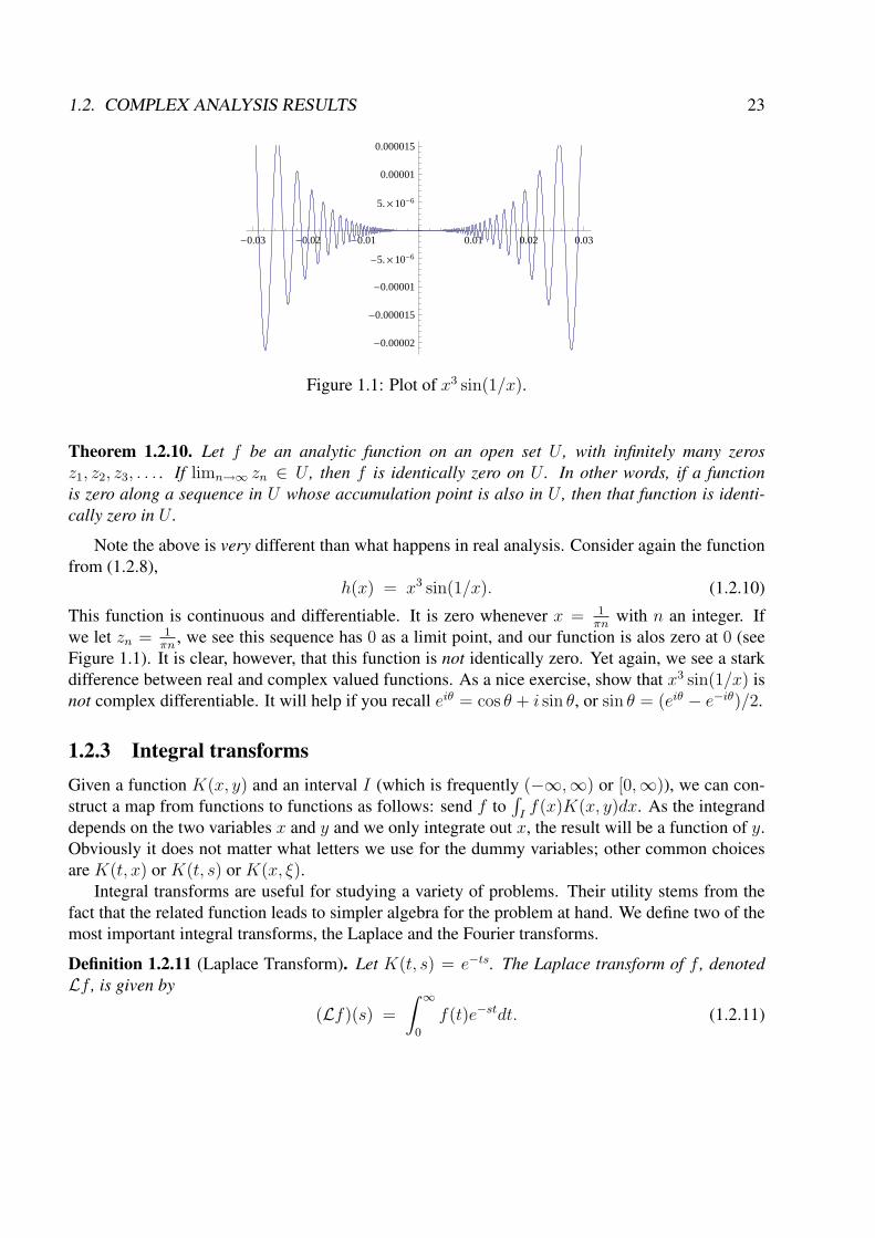
Figure 1.1: Plot of x3 sin(1/x).
Theorem 1.2.10. Let f be an analytic function on an open set U , with infinitely many zerosz1, z2, z3, . . . . If limn→∞ zn ∈ U , then f is identically zero on U . In other words, if a functionis zero along a sequence in U whose accumulation point is also in U , then that function is identi-cally zero in U .
Note the above is very different than what happens in real analysis. Consider again the functionfrom (1.2.8),
h(x) = x3 sin(1/x). (1.2.10)
This function is continuous and differentiable. It is zero whenever x = 1πn
with n an integer. Ifwe let zn = 1
πn, we see this sequence has 0 as a limit point, and our function is alos zero at 0 (see
Figure 1.1). It is clear, however, that this function is not identically zero. Yet again, we see a starkdifference between real and complex valued functions. As a nice exercise, show that x3 sin(1/x) isnot complex differentiable. It will help if you recall eiθ = cos θ + i sin θ, or sin θ = (eiθ − e−iθ)/2.
1.2.3 Integral transformsGiven a function K(x, y) and an interval I (which is frequently (−∞,∞) or [0,∞)), we can con-struct a map from functions to functions as follows: send f to
∫If(x)K(x, y)dx. As the integrand
depends on the two variables x and y and we only integrate out x, the result will be a function of y.Obviously it does not matter what letters we use for the dummy variables; other common choicesare K(t, x) or K(t, s) or K(x, ξ).
Integral transforms are useful for studying a variety of problems. Their utility stems from thefact that the related function leads to simpler algebra for the problem at hand. We define two of themost important integral transforms, the Laplace and the Fourier transforms.
Definition 1.2.11 (Laplace Transform). Let K(t, s) = e−ts. The Laplace transform of f , denotedLf , is given by
(Lf)(s) =
∫ ∞
0
f(t)e−stdt. (1.2.11)

24 CHAPTER 1. FROM GENERATING FUNCTIONS TO THE CENTRAL LIMIT THEOREM
Given a function g, its inverse Laplace transform, L−1g, is
(L−1g)(t) = limT→∞
1
2πi
∫ c+iT
c−iT
estg(s)ds = limT→∞
1
2πi
∫ T
−T
e(c+iτ)tg(c + iτ)idτ. (1.2.12)
Definition 1.2.12 (Fourier Transform). Let K(x, y) = e−2πixy. The Fourier transform of f , denotedFf or f , is given by
f(y) =
∫ ∞
−∞f(x)e−2πixydx, (1.2.13)
where
eiθ :=∞∑
n=0
θn
n!= cos θ + i sin θ. (1.2.14)
The inverse Fourier transform of g, denoted F−1g, is
(F−1g)(x) =
∫ ∞
−∞g(y)e2πixydy. (1.2.15)
Note other books define the Fourier transform differently, sometimes using K(x, y) = e−ixy orK(x, y) = e−ixy/
√2π.
Remark 1.2.13. The Laplace and Fourier transforms are related. If we let s = 2πiy and considerfunctions f(x) which vanish for x ≤ 0, we see the Laplace and Fourier transforms are equal.
Given a function f we can compute its transform. What about the other direction? If we are toldg is the transform of some function f , can we recover f from knowing g? If yes, is the correspondingf unique? Fortunately, the answer to both questions turns out to be ‘yes’, provided f and g satisfycertain nice conditions. A particularly nice set of functions to study is the Schwartz space.
Definition 1.2.14 (Schwartz space). The Schwartz space, S(R), is the set of all infinitely differen-tiable functions f such that, for any non-negative integers m and n,
supx∈R
∣∣∣∣(1 + x2)m dnf
dxn
∣∣∣∣ < ∞, (1.2.16)
where supx∈R |g(x)| is the smallest number B such that |g(x)| ≤ B for all x (think ‘maximum value’whenever you see supremum).
Theorem 1.2.15 (Inversion Theorems). ADD STUFF ON LAPLACE! Let f ∈ S(R), the Schwartzspace. Then
f(x) =
∫ ∞
−∞f(y)e2πixydy, (1.2.17)
where f is the Fourier transform of f . In particular, if f and g are Schwartz functions with the sameFourier transform, then f(x) = g(x).

1.2. COMPLEX ANALYSIS RESULTS 25
This interplay between a function and its transform will be very useful for us when we studyprobability distributions, as the moment generating function is an integral transform of the density!Recall the moment generating function is defined by MX(t) = E[etX ], or
MX(t) =
∫ ∞
−∞etxf(t)dt. (1.2.18)
If f(x) = 0 for x ≤ 0, this is just the Laplace transform of f . Alternatively, if we take t = −2πiythen it is the Fourier transform of f . This is trivially related to (yet another!) generating function,the characteristic function of X , which is defined by φ(t) = E[eitX ].
We now see why these results from complex analysis will save the day. The inversion formulasabove tell us that, if our initial distribution is nice, then knowing its integral transform is the sameas knowing it; in other words, knowing the integral transform uniquely determines the distribution.
1.2.4 Complex analysis and moment generating functionsWe conclude our technical digression by stating a few more very useful facts. The proof of theserequires properties of the Laplace transform, which is defined by (Lf)(s) =
∫∞0
e−sxf(x)dx. Thereason the Laplace transform plays such an important role in the theory is apparent when we recallthe definition of the moment generating function of a random variable X with density f :
MX(t) = E[etX ] =
∫ ∞
−∞etxf(x)dx; (1.2.19)
in other words, the moment generating function is the Laplace transform of the density evaluated at−s = t.
Before stating our results, we recall some notation.
Definition 1.2.16. Let FX and GY be the cumulative distribution functions of the random variablesX and Y with densities f and g. This means
FX(x) =
∫ x
−∞f(t)dt
GY (y) =
∫ y
−∞g(v)dv. (1.2.20)
Our results from complex analysis imply the following two very important and useful theo-rems for determining when we have enough information from the moments to uniquely determinea probability density.
Theorem 1.2.17. Assume the moment generating functions MX(t) and MY (t) exist in a neighbor-hood of zero (i.e., there is some δ such that both functions exist for |t| < δ). If MX(t) = MY (t)in this neighborhood, then FX(u) = FY (u) for all u. As the densities are the derivatives of thecumulative distribution functions, we have f = g.

26 CHAPTER 1. FROM GENERATING FUNCTIONS TO THE CENTRAL LIMIT THEOREM
Theorem 1.2.18. Let {Xi}i∈I be a sequence of random variables with moment generating functionsMXi
(t). Assume there is a δ > 0 such that when |t| < δ we have limi→∞ MXi(t) = MX(t) for some
moment generating function MX(t), and all moment generating functions converge for |t| < δ.Then there exists a unique cumulative distribution function F whose moments are determined fromMX(t) and for all x where FX(x) is continuous, limn→∞ FXi
(x) = FX(x).
The proof of these theorems follow from results in complex analysis, specifically the Laplaceand Fourier inversion formulas.
To give an example as to how the results from complex analysis allow us to prove results suchas these, we give most of the details in the proof of the next theorem. We deliberately do not try andprove the following result in as great generality as possible!
Theorem 1.2.19. Let X and Y be two continuous random variables on [0,∞) with continuousdensities f and g, all of whose moments are finite and agree. Suppose further that:
1. There is some C > 0 such that for all c ≤ C, e(c+1)tf(et) and e(c+1)tg(et) are Schwartzfunctions (see Definition 1.2.14). This is not a terribly restrictive assumption; f and g needto have decay in order for all moments to exist and be finite. As we are evaluating f and g atet and not t, there is enormous decay here. The meat of the assumption is that f and g areinfinitely differentiable and their derivatives decay.
2. The (not necessarily integral) moments
µ′rn(f) =
∫ ∞
0
xrnf(x)dx and µ′rn(g) =
∫ ∞
0
xrng(x)dx (1.2.21)
agree for some sequence of non-negative real numbers {rn}∞n=0 which has a finite accumula-tion point (i.e., limn→∞ rn = r < ∞).
Then f = g (in other words, knowing all these moments uniquely determines the probabilitydensity).
Proof. We sketch the proof. Let h(x) = f(x)− g(x), and define
A(z) =
∫ ∞
0
xzh(x)dx. (1.2.22)
Note that A(z) exists for all z with real part non-negative. To see this, let Re(z) denote the real partof z, and let k be the unique non-negative integer with k ≤ Re(z) < k +1. Then xRez ≤ xk +xk+1,and
|A(z)| ≤∫ ∞
0
xRe(z) [|f(x)|+ |g(x)|] dx
≤∫ ∞
0
(xk + xk+1)f(x)dx +
∫ ∞
0
(xk + xk+1)g(x)dx = 2µ′k + 2µ′k+1. (1.2.23)

1.2. COMPLEX ANALYSIS RESULTS 27
Results from analysis now imply that A(z) exists for all z. The key point is that A is also differen-tiable. Interchanging the derivative and the integration (which can be justified), we find
A′(z) =
∫ ∞
0
xz(log x)h(x)dx. (1.2.24)
To show that A′(z) exists, we just need to show this integral is well-defined. There are only twopotential problems with the integral, namely when x →∞ and when x → 0. For x large, xz log x ≤xdRe(z)e (where ewd is the smallest integer at least as large as w) and thus
∣∣∫∞1
xz(log x)h(x)dx∣∣ <
∞. For x near 0, h(x) looks like h(0) plus a small error (remember we are assuming f and gcontinuous). There is a constant Cf,g such that
limε→0
∫ 1
ε
∣∣∣∣∫ ∞
0
xz(log x)h(x)dx
∣∣∣∣ ≤ limε→0
∫ 1
ε
(log x)Cf,gdx; (1.2.25)
the reason it is less than or equal to the right hand side is that Re(z) > 0 so |xz| ≤ 1, and sincef and g are Schwartz functions they are bounded. The anti-derivative of log x is x log x − x, andlimε→0(ε log ε− ε)s = 0. This is enough to prove that this integral is bounded, and thus from resultsin analysis we get A′(z) exists.
We (finally!) use our results from complex analysis. As A is differentiable once, it is infinitelydifferentiable and it equals its Taylor series for z with Re(z) > 0. Therefore A is an analyticfunction which is zero for a sequence of zn’s with an accumulation point, and thus it is identicallyzero. This is amazing – initially we only knew A(z) was zero if z was a positive integer or if z wasin the sequence {rn}; we now know it is zero for all z with Re(z) > 0.
We change variables, and replace x with et and dx with etdt. The range of integration is now−∞ to ∞, and we set h(t)dt = h(et)etdt. We now have
A(z) =
∫ ∞
−∞etzh(t)dt = 0. (1.2.26)
Choosing z = c + 2πiy with c less than the C from our hypotheses gives
A(c + 2πiy) =
∫ ∞
−∞e2πity
[ecth(t)
]dt = 0. (1.2.27)
Our assumptions imply that ecth(t) is a Schwartz function, and thus it has a unique inverse Fouriertransform. As we know this transform is zero, it implies that ecth(t) = 0, or h(x) = 0, or f(x) =g(x).
Remark 1.2.20. What if we lessen our restrictions on f and g; perhaps one of them is not contin-uous? Perhaps there is a unique continuous probability distribution attached to a given sequenceof moments such as in the above theorem, but if we allow non-continuous distributions there couldbe additional possibilities. This topic is beyond the scope of this book, requiring more advancedresults from analysis; however, we wanted to point out where the dangers lie, where we need to becareful.

28 CHAPTER 1. FROM GENERATING FUNCTIONS TO THE CENTRAL LIMIT THEOREM
Exercise 1.2.21. If we are told that all the moments of f are finite and f is infinitely differentiable,must there be some C such that for all c < C we have e(c+1)tf(et) is a Schwartz function?
After proving Theorem 1.2.19, it’s natural to go back to the two densities that are causing somuch trouble, namely (see (1.1.49))
f1(x) =1√
2πx2e−(log2 x)/2
f2(x) = f1(x) [1 + sin(2π log x)] . (1.2.28)
We know these two densities have the same integral moments (their kth moments are ek2/2 for k anon-negative integer). These functions have the correct decay; note
e(c+1)tf1(et) = e(c+1)t · e−t2/2
√2πet
, (1.2.29)
which decays fast enough for any c to satisfy the assumptions of Theorem 1.2.19. As these twodensities are not the same, some condition must be violated. The only condition left to check iswhether or not we have a sequence of numbers {rn}∞n=0 with an accumulation point r > 0 such thatthe rn
th moments agree. Using complex analysis (specifically, contour integration), we can calculatethe (a + ib)thmoments. We find
(a + ib)th moment of f1 is e(a+ib)2/2 (1.2.30)
and
(a + ib) moment of f1 is e(a+ib)2/2 +i
2
(e(a+i(b−2π))2/2 − e(a+i(b+2π))2/2
). (1.2.31)
While these moments agree for b = 0 and a a positive integer, there is no sequence of real momentshaving an accumulation point where they agree. To see this, note that when b = 0 the athmoment off2 is
ea2/2 + e(a−2iπ)2/2(1− e4iaπ
), (1.2.32)
and this is never zero unless a is a half-integer (i.e., a = k/2 for some integer k). In fact, the reasonwe wrote (1.2.32) as we did was to highlight the fact that it is only zero when a is a half-integer.Exponentials of real or complex numbers are never zero, and thus the only way this can vanish isif 1 = e4iaπ. Recalling that eiθ = cos θ + i sin θ, we see that the vanishing of the athmoment isequivalent to 1 − cos(4πa) − i sin(4πa) = 0; the only way this can happen is if a = k/2 for somek. If this happens, the cosine term is 1 and the sine term is 0.
1.3 The Central Limit Theorem
1.3.1 Means, Variances and Standard DeviationsThe Central Limit Theorem is one of the true gems of probability. The hypotheses are quite weak,and are frequently met in practice. What is so amazing is the universality of the result. Before

1.3. THE CENTRAL LIMIT THEOREM 29
stating the Central Limit Theorem, we set some notation and motivate why we study the quantitieswe do.
Recall that the mean µ and variance σ2 of a random variable X with density f is given by
µ = E[X] =
∫ ∞
−∞xf(x)dx
σ2 = E[(X − µ)2] =
∫ ∞
−∞(x− µ)2dx (1.3.1)
if X is a continuous random variable, and
µ = E[X] =∞∑
n=1
xnf(xn)
σ2 = E[(X − µ)2] =∞∑
n=1
(xi − µ)2 (1.3.2)
if X is discrete. We often write Var(X) for the variance of X . The mean measures the averagevalue of X , and the variance how spread out it is (the larger the variance, the more spread out thedensity).
Example 1.3.1. Consider the following two data sets:
S1 = {0, 0, 0, 0, 0, 0, 0, 0, 0, 0, 100, 100, 100, 100, 100, 100, 100, 100, 100, 100}S2 = {50, 50, 50, 50, 50, 50, 50, 50, 50, 50, 50, 50, 50, 50, 50, 50, 50, 50, 50, 50}. (1.3.3)
Both data sets have a mean of 50, but the first is clearly more spread out than the second. If we try tocompute the variances of these two sets, we run into a problem, namely: what are the probabilitiesf(xi)? Unless there is information to the contrary, one typically assumes that all data points areequally likely. There are two ways now to determine the probabilities. The first way is to treat eachobservation as a different measurement. In that case, we have x1 = x2 = · · · = x10 = 0, all withprobabilities 1/20, and x11 = x12 = · · ·x20 = 100, all with probability 1/20. Alternatively, wecould consider x1 = 0 with probability 1/2 and x2 = 100 with probability 1/2. Note, however, thatwhile the number of data points is different in the two interpretations, all computed quantities willbe the same. For example, let’s calculate the variance using both methods. Using the first, we findthe variance is
10∑n=1
(0− 50)2 · 1
20+
20∑n=11
(100− 50)2 · 1
20= 10 · 502 · 1
20+ 10 · 502 · 1
20= 502, (1.3.4)
while the second method gives
(0− 50)2 · 1
2+ (100− 50)2 · 1
2= 502. (1.3.5)
The second set, S2, is significantly easier to compute. All values are the same, and thus the varianceis clearly zero.
30 CHAPTER 1. FROM GENERATING FUNCTIONS TO THE CENTRAL LIMIT THEOREM
Not surprisingly, the second data set has significantly smaller variance than the first; however,there is something a bit unsettling about using the variance to quantify how spread out a data setis. The difficulty comes when our numbers have physical meaning. For example, imagine the twodata sets are recording how wait time (in seconds) for a bank teller. Thus we either have a wait of0 seconds, of 50 seconds, or of 100 seconds. In both banks the average waiting time of customersis the same; however, in the second bank all customers have the same experience, while in thefirst some are presumably very happy with no wait, while others are almost surely upset at a verylong wait. This can be seen by noting the variance in the second set is zero while in the first it is502 = 2500; however, it is not quite right to say this. In this situation, there are units attached tothe variance. As time is measured in seconds, the variance is measured in seconds-squared. To behonest, I have no real clue what a second-squared is. I can imagine a meter-squared (area), but asecond-squared? Yet this is precisely the unit that arises here. To see this, note that the xi and µ aremeasured in seconds, the probabilities are unitless numbers, so the variance is a sum of expressionssuch as (0sec− 50sec)2, (50sec− 50sec)2 and (100sec− 50sec)2. Thus, the variance is measured insecond-squared.
If I want to find out how long I need to wait, I’m expecting an answer such as ‘say 10 minutes,plus or minus a minute or two’. I’m not expecting anyone to respond with ‘say 10 minutes, witha variance of 1 or four minutes-squared’. Fortunately, there is a simple solution to this problem;instead of reporting the variance, it is frequently more appropriate to report the standard deviation,which is the square-root of the variance.
Returning to our earlier example, we would say that for the first data set, the mean wait time was50 seconds, with a standard deviation of 50 seconds, while in the second it was also a mean waittime of 50 seconds, but with a standard deviation of 0 seconds.
The point of the above is that the standard deviation and the mean have the same units, whilethe variance and the mean do not; we always want to compare apples and apples (i.e., objects withthe same dimensions). In fact, this is why the notation for the variance is σ2, highlighting the factthat the quantity we will frequently care about is σ, its square-root. Similar to writing Var(X) forthe variance of X , we occasionally write StDev(X) for its standard deviation.
1.3.2 Normalizations
In the previous subsection we saw that the variance of a random variable is not the right scale tolook at fluctuations, as the units were wrong. In particular, if X is measured in seconds then thevariance is in the physically mysterious unit of seconds-squared; it is the standard deviation that hasthe same units, and thus it is the standard deviation that we use to discuss how spread out a data setis.
Finding the correct scale or units to discuss a problem is very important. For example, imag-ine we have two sections of calculus with identical students in each but very different professors(admittedly this is not an entirely realistic situation as no two classes are identical; however, if theclasses are large then this is approximately true). Let’s assume one professor writes really easyexams, and another writes very challenging ones. If we’re told that Hari from the first section has

1.3. THE CENTRAL LIMIT THEOREM 31
a 92 average and Daneel from the second section has an 84, which is the better student? Withoutmore information, it is very hard to judge – how does a 92 in the ‘easier’ section compare to an ‘84’in the harder?
Let’s assume we know more about the two classes. Let’s say that in section 1 (the one withthe easier exams) the average grade is a 97 and the standard deviation is 1, while in section 2 theaverage grade is a 64 and the standard deviation is 10. Once we know this, it’s clear that Daneel isthe superior student (remember in this pretend example we’re assuming the two classes are identicalin terms of ability; the only difference is that one takes easier tests than the other). Hari is actuallybelow average (by 5 standard deviations, a sizeable number), while Daneel is significantly aboveaverage (by 2 standard deviations).
We are warned about comparing apples and oranges, and that’s what happened here – we havetwo different scales, and an 84 on one scale does not mean the same as an 84 on the other. To avoidproblems like this (i.e., to compare apples and apples), we frequently normalize our data to havemean zero and variance 1. This puts different data sets on the same scale. This is done as follows:
Definition 1.3.2 (Normalization of a random variable). Let X be a random variable with mean µand standard deviation σ, both of which are finite. The normalization, Y , is defined by
Y :=X − E[X]
StDev(X)=
X − µ
σ. (1.3.6)
Note thatE[Y ] = 0 and StDev(Y ) = 1. (1.3.7)
Remark 1.3.3. Instead of calling the above a normalization we could call it a standardization ora renormalization; after some thought we decided to call it a normalization. One reason is thatthis process is used all the time in problems involving the Central Limit Theorem, and thus this issetting the stage for the result there (which involves the normal distribution). For a typical X thenormalization will not be normally distributed.
The normalization process we’ve discussed is quite natural; it rescales any ’nice’ random vari-able to a new one having mean 0 and variance 1. The only assumption we need is that it havefinite mean and standard deviation. This a mild assumption, but not all distributions satisfy it. Forexample, consider the Cauchy distribution
f(x) =1
π
1
1 + x2. (1.3.8)
It is debateable whether or not this distribution has a mean; it clearly doesn’t have a finite variance.Why is the mean of this distribution problematic? It’s because we have an improper integral wherethe integrand is sometimes positive and sometimes negative. This means how we go to infinitymatters. For example,
limA→∞
∫ A
−A
xdx
π(1 + x2)= lim
A→∞0 = 0, (1.3.9)

32 CHAPTER 1. FROM GENERATING FUNCTIONS TO THE CENTRAL LIMIT THEOREM
while
limA→∞
∫ 2A
−A
xdx
π(1 + x2)= lim
A→∞
∫ 2A
A
xdx
π(1 + x2), (1.3.10)
and the last integral is, for A enormous, essentially∫ 2A
Adx/x = log(2A)− log(A) = log(2). Thus,
how we tend to infinity matters!
Remark 1.3.4. We cannot stress enough how important and useful it is to normalize a randomvariable. We will discuss this again below, but given any random variable X , sending X to(X − E[X])/StDev(X) is an extremely natural and often useful thing to do.
1.3.3 Statement of the Central Limit TheoremOf the many distributions encountered in probability, perhaps the most important is the normaldistribution. One way to measure how important a distribution is to a subject is to count howmany different names are used to refer to it; in this case, names include the normal distribution, theGaussian distribution and the bell curve.
Definition 1.3.5 (Normal distribution). A random variable X is normally distributed (or has thenormal distribution, or is a Gaussian random variable) with mean µ and variance σ2 if the densityof X is
f(x) =1√
2πσ2exp
(−(x− µ)2
2σ2
). (1.3.11)
We often write X ∼ N(µ, σ2) to denote this. If µ = 0 and σ2 = 1, we say X has the standardnormal distribution.
There are many versions of the Central Limit Theorem. The differences range from the hy-potheses assumed and the type of convergence obtained; not surprisingly, the more nice propertiesone assumes, the stronger the convergence. We state a theorem which, while not the most generalone possible, is easy to state and has hypotheses satisfied by most of the common distributions weencounter.
Theorem 1.3.6 (Central Limit Theorem). Let X1, . . . , XN be independent, identically distributedrandom variables whose moment generating functions converge for |t| < δ for some δ > 0 (thisimplies all the moments exist and are finite). Denote the mean by µ and the variance by σ2, let
XN =X1 + · · ·+ XN
N(1.3.12)
and set
ZN =XN − µ
σ/√
N. (1.3.13)
Then as N →∞, the distribution of ZN converges to the standard normal (see Definition 1.3.5 fora statement).

1.3. THE CENTRAL LIMIT THEOREM 33
One way to interpret the above is as follows: imagine X1, . . . , XN are N independent measure-ments of some process or phenomenon. Then XN is the average of the observed values. As the Xi’sare drawn from a common distribution with mean µ, and as expectation is linear, we have
E[XN ] = E[X1 + · · ·+ XN
N
]=
1
N
N∑n=1
E[Xn] =1
N·Nµ = µ. (1.3.14)
Since the Xn’s are independent, the variance of XN is
Var(XN) = Var
(X1 + · · ·+ XN
N
)=
1
N2
N∑n=1
Var(Xn) =1
N2·Nσ2 =
σ2
N, (1.3.15)
so the standard deviation of XN is just σ/√
N . Note as N → ∞ the standard deviation of XN
tends to zero. This leads to the following interpretation: as we take more and more measurements,the distribution of the average value is living in a tighter and tighter band about the true mean. Wechose to write XN for the average value of the Xn’s to emphasize that we have a sum of N randomvariables.
Most probability books have tables with the values of the standard normal. For example, imag-ine we want to compute the probability that a random variable with the standard normal distributionis within one standard deviation of 0. We can just turn to the back of the book and grab this infor-mation; however, it is extremely unlikely you’ll ever find a book with the tabulation of probabilitiesfor a normally distributed random variable with mean
√2 and variance π.
Why aren’t there such tables? There are two reasons today. The first, of course, is that computersare very powerful and accessible, and thus the need for printed tables like the last one alluded to isgreatly lessened, as a few lines of code will give us the answer. While this might be a satisfactoryanswer today, why were there no such tables before computers? Perhaps our example is a bit absurd,but what about a normally distributed random variable with mean 0 and variance 4; surely that musthave occurred in someone’s research?
The reason we don’t need such tables is that, if we know the probabilities for the standardnormal, we can use those to compute the probabilities for any normally distributed random variable.For definiteness, imaging W ∼ N(3, 4), which means W has a mean of 3 and a variance of 4 (or astandard deviation of 2). Imagine we want to know the probability that W ∈ [2, 10]. We normalizeW (see Definition 1.3.2) by setting
Z =W − E[W ]
StDev(W )=
W − 3
2. (1.3.16)
Thus asking that W ∈ [2, 10] is equivalent to asking Z to be in a certain interval. Which interval?Well, W ∈ [2, 10] is the same as Z ∈ [−1/2, 7/2]. If we have a table of probabilities for the standardnormal, we can now compute this probability, and hence find the probability that W ∈ [2, 10].
We thus see that we need only have one table of probabilities for one normally distributed ran-dom variables, as we can deduce the probabilities for any other with simple algebra. In the days

34 CHAPTER 1. FROM GENERATING FUNCTIONS TO THE CENTRAL LIMIT THEOREM
before computers, this was a very important observation. It meant people needed only calculate onetable of probabilities in order to study any normally distribution.
This is very similar to logarithm tables. Most books only had logarithms base e (sometimes base10 was given, or perhaps base 2). Through a similar normalization process, if we have a table oflogarithms in one base we can compute logarithms in any base. This is because of the followinglog-law (commonly called the Change of Variable formula): For any b, c, x > 0 we have
logc x =logb x
logb c. (1.3.17)
Imagine we know logarithms base b. Then using the right hand side of the above formula, we cancompute the logarithm of any x base c. Thus it suffices to compile just one table of logarithms (asbase e and base 10 are often both used, it might be a kindness to assemble both tables, but just onewould suffice).
Before proving the Central Limit Theorem, we’ll analyze some special cases where the proof issimpler. As our hypotheses include statements about moment generating functions, it should comeas no surprise that we’ll need to know the moment generating function of the standard normal.
Theorem 1.3.7 (Moment generating function of normal distributions). Let X be a normal randomvariable with mean µ and variance σ2. Its moment generating function satisfies
MX(t) = eµt+σ2t2
2 . (1.3.18)
In particular, if Z has the standard normal distribution, its moment generating function is
MZ(t) = et2/2. (1.3.19)
Sketch of the proof. While we could try to directly compute MX(t) through MX(t) = E[etX ],clearly we would much rather compute MZ(t) = E[etZ ]. The reason is clear: Z has zero meanand variance 1, and thus the numbers are a little cleaner. We could set up the equation for MX(t)and then do some change of variables, or we could note that we can deduce MX(t) from MZ(t)through part (2) of Theorem 1.1.19. Specifically, we have
Z =X − µ
σ, (1.3.20)
or equivalentlyX = σZ + µ. (1.3.21)
We then use MαZ+β(t) = eβtMZ(αt).Thus we are reduced to computing MZ(t), or
MZ(t) = E[etZ ] =
∫ ∞
−∞etz · e−z2/2dx√
2π. (1.3.22)

1.3. THE CENTRAL LIMIT THEOREM 35
We solve this by completing the square. The argument of the exponential is
tz − z2
2= −z2 − 2tz
2= −z2 − 2tz + t2 − t2
2= −(z − t)2
2+
t2
2. (1.3.23)
Note the second term is independent of z, the variable of integration. We find
MZ(t) =
∫ ∞
−∞
1√2π
exp
(−(z − t)2
2+
t2
2
)dz
= et2/2
∫ ∞
−∞
e−(z−t)2/2dz√2π
= et2/2
∫ ∞
−∞
e−u2/2du√2π
= et2/2, (1.3.24)
as the last integral is 1 as it is the integral of the standard normal’s density from −∞ to ∞.
1.3.4 Proof of the CLT for sums of Poisson random variables via MGFAs a warm-up for the general proof, we’ll show that the normalized sum of Poisson random variablesconverges to the standard normal distribution. The proof will include the key ideas of the generalcase, and will involve moment generating functions. We know from Theorem 1.3.7 that the momentgenerating function of the standard normal is et2/2. We computed the moment generating functionof a Poisson random variable X with mean λ in Example 1.1.20. We showed that it is
MX(t) = eλ(et−1) = 1 + µt +µ′2t
2
2!+ · · · . (1.3.25)
Note the mean is λ and the variance is λ. To see this, we differentiate the moment generatingfunction and then set t = 0:
µ =dMX
dt
∣∣∣t=0
=(λet · eλ(et−1)
) ∣∣∣t=0
= λ
µ′2 =d2MX
dt2
∣∣∣t=0
=(λet · eλ(et−1) + λ2e2t · eλ(et−1)
) ∣∣∣t=0
= λ + λ2; (1.3.26)
asσ2 = E[(X − µ)2] = E[X2]− E[X]2, (1.3.27)
we see thatσ2 = (λ + λ2)− λ2 = λ. (1.3.28)
Remark 1.3.8. Alternatively, we could have found the mean and variance by Taylor expanding themoment generating function. We would have
eλ(et−1) = 1 + λ(et − 1) +(λ(et − 1))2
2!+
(λ(et − 1))3
3!+ · · · . (1.3.29)
36 CHAPTER 1. FROM GENERATING FUNCTIONS TO THE CENTRAL LIMIT THEOREM
While at first this looks very complicated, we note that a Taylor expansion of et−1 gives t+ t2/2!+· · · = t(1 + t/2 + · · · ); in other words, (et − 1)k is divisible by tk. This means
eλ(et−1) = 1 + λt
(1 +
t
2+ · · ·
)+ λ2t2
(1 + t/2 + · · · )2
2!+ λ3t3
(1 + t/2 + · · · )3
3!+ · · ·
= 1 + λt + λt2
2+ λ
t2
2+ terms in t3 or higher
= 1 + λt +λ2t2
2+ · · · . (1.3.30)
Thus, by knowing the Taylor series expansion of ex, we can find the first two moments throughalgebra and avoid differentiation; we leave it to the reader to determine which approach they likemore (or hate less!).
Theorem 1.3.9. Let X,X1, . . . , XN be Poisson random variables with parameter λ. Let
XN =X1 + · · ·+ XN
N, ZN =
XN − E[XN ]
StDev(XN). (1.3.31)
Then as N →∞, ZN converges to having the standard normal distribution.
Proof. We expect XN to be approximately equal to the mean of the Poisson random variable, whichin this case is λ. This follows from the linearity of expected value:
E[XN ] = E[X1 + · · ·+ XN
N
]=
1
N
N∑n=1
E[Xi] =1
N·Nλ = λ. (1.3.32)
We will write µ for the mean (and not λ); this keeps the argument a bit more general, and theresulting calculations will look like the general case for a bit longer if we do this.
Let σ2 denote the variance of the Xn’s (Poisson distributions with parameter λ). We knowσ =
√λ; however, we again choose to write σ below so that these calculations will look a lot like
the general case. The variance of XN is computed similarly; since the Xn are independent we have
Var(XN) = Var
(X1 + · · ·+ XN
N
)=
1
N2
N∑n=1
Var(Xn) =1
N2·Nσ2 =
σ
N. (1.3.33)
As always, the natural quantity to study is
ZN =XN − E[XN ]
StDev(XN)=
X1+···+XN
N− µ
σ/√
N=
(X1 + · · ·+ XN)−Nµ
σ√
N. (1.3.34)
We now useMX+a
b(t) = eat/bMX(t/b) (1.3.35)

1.3. THE CENTRAL LIMIT THEOREM 37
and the moment generating function of a sum of independent variables is the product of the momentgenerating (Theorem 1.1.19) functions to find the moment generating function of ZN . We have
MZN(t) = M (X1+···+XN )−Nµ
σ√
N
(t)
= M∑Nn=1
Xn−µ
σ√
N
(t)
=N∏
n=1
MXn−µ
σ√
N
(t)
=N∏
n=1
e−µt
σ√
N MX
(t
σ√
N
)
=N∏
n=1
e−µt
σ√
N eµ
(e
tσ√
N −1)
, (1.3.36)
where in the final step we take advantage of knowing the moment generating function of MX(t).We now Taylor expand the exponential, using
eu =∞∑
k=0
uk
k!= 1 + u +
u2
2!+
u3
3!+ · · · . (1.3.37)
This is one of the most important Taylor expansion we will encounter. Thus the exponential in(1.3.36) is
et
σ√
N = 1 +t
σ√
N+
t2
2σ2N+
t3
6σ3N√
N+ · · · . (1.3.38)
The important thing to note is that after subtracting 1, the first piece is tσ√
N, the next piece is t2
2σ2N,
and the remaining pieces are dominated by a geometric series (starting with the cubed term) withr = t
σ√
N. Thus, the contribution from all the other terms is of size at most some constant times
t3
N√
N. For large N this will be negligible, and we write errors like this as O
(t3
N√
N
). (This is
called big-Oh notation. The technical definition of f(x) = O(g(x)) is that there are constants C, x0
such that whenever x > x0, |f(x)| ≤ Cg(x). In other words, from some point onward |f(x)| isdominated by a constant times g(x).)
Thus (1.3.36) becomes
MZN(t) =
N∏n=1
e−µt
σ√
N eλ·
(t
σ√
N+ t2
2σ2N+O
(t3
N√
N
))
=N∏
n=1
eµt2
σ2N+O
(t3
N√
N
)
= et2
2+O
(t3√N
)(1.3.39)

38 CHAPTER 1. FROM GENERATING FUNCTIONS TO THE CENTRAL LIMIT THEOREM
where the last line follows from the fact that we have a product over N identical terms, and as themean µ = λ and the variance σ2 = λ (for X Poisson with parameter λ), we see µ
σ2 = 1. Thus,
for all t, as N → ∞ the moment generating function of ZN tends to et2
2 , which is the momentgenerating function of the standard normal. The proof is completed by invoking Theorem 1.2.18,one of our black-box results from complex analysis, which states that if a sequence of momentgenerating functions which exist for |t| < δ converges to a moment generating function of a density,then the corresponding density converges to that density. In our case, this implies convergence tothe standard normal.
Remark 1.3.10. We only need to Taylor expand far enough to get the main term (which has a finitelimit as N →∞) and then estimate the size of the error term (which tends to zero as N →∞).
Even though this was a special case, some features are visible here that will reappear when weconsider the general case. Note that the higher moments of the distribution don’t seem to matter; allwe used was the first and second moments of X . The higher moments do matter; their affect is tocontrol the rate of convergence to the standard normal. They are felt in the eO(t3/
√N) term.
1.3.5 Proof of the CLT for general sums via MGFWe deliberately kept the proof of Theorem 1.3.9 (normalized sums of independent identically dis-tributed Poisson random variables converges to the standard normal) as general as possible as longas possible for use in proving the full version of the Central Limit Theorem.
Proof of Theorem 1.3.6 (the Central Limit Theorem). Looking at the proof of Theorem 1.3.9, ourarguments held for any distribution up until the last line of (1.3.36), where we finally used the factthat we had independent Poisson random variables by substituting for MX(t/σ
√N). This time, we
can’t substitute a specific expansion for MX(t/σ√
N) as we don’t know MX . We thus have
MZN(t) =
N∏n=1
e−µt
σ√
N MX
(t
σ√
N
)= e
−µt√
Nσ MX
(t
σ√
N
)N
(1.3.40)
(as the random variables are identically distributed).There are several ways to do the algebra to finish the proof; we chose the following approach as it
emphasizes one of the most important tricks in mathematics. Namely, whenever you see a productyou should seriously consider replacing it with a sum. The reason is we have lots of experienceevaluating sums. We have formulas for special sums, and using Taylor series we can expand nicefunctions as sums. We don’t really know that many products, or expansions of functions in terms ofproducts.
How do we convert a product to a sum? We know the logarithm of a product is the sum of thelogarithms. Thus, let’s take logarithms of (1.3.40), and then when we’re done analyzing it we justexponentiate. We find
log MZN(t) = −µt
√N
σ+ N log MX
(t
σ√
N
). (1.3.41)

1.3. THE CENTRAL LIMIT THEOREM 39
Note the first term in the expansion above is of size√
N for fixed t; if it isn’t cancelled by somethingfrom the other term, the limit won’t exist. Forunately it is cancelled, and all we will care about isterms up to size 1/N . We need to be concerned with terms this small because we multiply by N ;however, terms of size 1/N3/2 or smaller won’t contribute in the limit as they are only multipliedby N , and thus are still small.
We know
MX(t) = 1 + µt +µ′2t
2
2!+ · · · = 1 + t
(µ +
µ′2t2
+ · · ·)
. (1.3.42)
We now use the Taylor series expansion for log(1 + u), which is
log(1 + u) = u− u2
2+
u3
3!− · · · . (1.3.43)
Combining the two gives
log MX(t) = t
(µ +
µ′2t2
+ · · ·)−
t2(µ +
µ′2t
2+ · · ·
)2
2+ · · ·
= µt +µ′2 − µ2
2t2 + terms in t3 or higher. (1.3.44)
Thus
log MX
(t
σ√
N
)= µt +
µ′2 − µ2
2t2 + terms in t3 or higher. (1.3.45)
But we do not want to evaluate MX at t, but rather at t/σ√
N . We find
log MX
(t
σ√
N
)=
µt
σ√
N+
µ′2 − µ2
2
t2
σ2N+ terms in t3/N3/2 or lower in N. (1.3.46)
Henceforth we’ll denote these lower order terms by O(N−3/2), and when we multiply these by Nwe’ll denote the new error by O(N−1/2). The entire point of all of this is to simplify (1.3.41), theexpansion for log MZN
(t). Collecting our pieces, we find
log MZN(t) = −µt
√N
σ+ N
(µt
σ√
N+
µ′2 − µ2
2
t2
σ2N+ O(N−3/2)
)
= −µt√
N
σ+
µt√
N
σ+
µ′2 − µ2
2
t2
σ2+ O(N−1/2)
=t2
2+ O(N−1/2). (1.3.47)
Why is the last step true? We have µ′2 − µ2; this equals E[X2] − E[X]2, which is an alternate wayof defining the variance. Thus µ′2 − µ2 = σ2, and the claim follows.

40 CHAPTER 1. FROM GENERATING FUNCTIONS TO THE CENTRAL LIMIT THEOREM
So, if log MZN(t) is like t/2 + O(N−1/2), then
MZN(t) = e
t2
2+O(N−1/2). (1.3.48)
Though we took a different route, we end in the same place as in the proof of Theorem 1.3.9. Weagain appeal to Theorem 1.2.18, one of our black-box results from complex analysis, which statesthat if a sequence of moment generating functions which exist for |t| < δ converges to a momentgenerating function of a density, then the corresponding density converges to that density. In ourcase, this implies convergence to the standard normal.
1.4 Fourier Analysis and the Central Limit TheoremAny theorem as important as the Central Limit Theorem deserves more than one proof. Differentproofs emphasize different aspects of the problem. Our first proof was based on properties of theinverse Laplace transform, specifically an appeal to Theorem 1.2.18. The proof below uses theFourier transform. It is thus very similar to the previous proof, as the Fourier transform and theLaplace transform are equal for certain functions after a change of variable. We choose to presentthis proof as well for several reasons. ADD REASONS!
1.4.1 Needed results from Fourier analysisRecall the Fourier transform of f is (see Definition 1.2.12)
f(y) =
∫ ∞
−∞f(x)e−2πixydx; (1.4.1)
(sometimes the Fourier transform is defined with e−ixy or eixy/√
2π instead of e−2πixy, so al-ways check the convention when you reference a book or use a program such as Mathematica).While f(y) is well defined whenever
∫∞−∞ |f(x)|dx < ∞, much more is true for functions with∫∞
−∞ |f(x)|2dx < ∞. Unfortunately, for many applications even this assumption isn’t enough, andwe need to take f in the Schwartz Space S(R) (see Definition 1.2.14), the space of all infinitelydifferentiable functions whose derivatives are rapidly decreasing. One can show the Fourier trans-form of a Schwartz function is a Schwartz function, and we have the following wonderful theoremon inverting the Fourier transform (Theorem 1.2.15), which for convenience we restate below.
Theorem 1.2.15 (Fourier Inversion Formula). For f ∈ S(R),
f(x) =
∫ ∞
−∞f(y)e2πixydy. (1.4.2)
In fact, for any f ∈ S(R), ∫ ∞
−∞|f(x)|2dx =
∫ ∞
−∞|f(y)|2dy. (1.4.3)

1.4. FOURIER ANALYSIS AND THE CENTRAL LIMIT THEOREM 41
Definition 1.4.1 (Compact Support). A function f : R→ C has compact support if there is a finiteclosed interval [a, b] such that for all x 6∈ [a, b], f(x) = 0.
Remark 1.4.2 (Advanced). Schwartz functions with compact support are extremely useful in manyarguments. It can be shown that given any continuous function g on a finite closed interval [a, b],there is a Schwartz function f with compact support arbitrarily close to g; i.e., for all x ∈ [a, b],|f(x) − g(x)| < ε. Similarly, given any such continuous function g, one can find a sum of stepfunctions of intervals arbitrarily close to g (in the same sense as above). Often, to prove a result forstep functions it suffices to prove the result for continuous functions, which is the same as provingthe result for Schwartz functions. Schwartz functions are infinitely differentiable and as the FourierInversion formula holds, we can pass to the Fourier transform space, which is sometimes easier tostudy.
Example 1.4.3. Whenever we define a space or a set, it’s worthwhile to show that it isn’t empty!Let’s show there are infinitely many Schwartz functions. We claim the Gaussians f(x) = 1√
2πσ2e−(x−µ)2/2σ2
are in S(R) for any µ, σ ∈ R. By a change of variables, it suffices to study the special case of µ = 0and σ = 1. Clearly the standard normal, f(x) = 1√
2πe−x2/2 is infinitely differentiable. Its first few
derivatives are
f ′(x) = −x · 1√2π
e−x2/2
f ′′(x) = (x2 − 1) · 1√2π
e−x2/2
f ′′′(x) = −(x3 − 3x) · 1√2π
e−x2/2. (1.4.4)
By induction, we can show that the nthderivative is a polynomial pn(x) of degree n times 1√2π
e−x2/2.To show f is Schwartz, by Definition 1.2.14 we must show
∣∣∣∣(1 + x2)m · pn(x)1√2π
e−x2/2
∣∣∣∣ (1.4.5)
is bounded. This follows from the fact that the standard normal decays faster than any polynomial.Say we want to show |xme−x2/2| is bounded. The claim is clear for |x| ≤ 1. What about larger |x|?We know ex2/2 ≥ (x2/2)k/k! for any k, so e−x2/2 ≤ k!2k/x2k. Thus |xme−x2/2| ≤ k!2k/x2k−m, andif we choose 2k > m then this is bounded by k!2k.
Exercise 1.4.4. Let f(x) be a Schwartz function with compact support contained in [−σ, σ] anddenote its Fourier transform by f(y). Prove for any integer A > 0 that |f(y)| ≤ cfy
−A, where theconstant cf depends only on f , its derivatives and σ. As such a bound is useless at y = 0, one oftenderives bounds of the form |f(y)| ≤ cf
(1+|y|)A .

42 CHAPTER 1. FROM GENERATING FUNCTIONS TO THE CENTRAL LIMIT THEOREM
1.4.2 Convolutions and Probability Theory
An important property of the Fourier transform is that it behave nicely under convolution. Remem-ber we denote the convolution of two functions f and g by h = f ∗ g, where
h(y) =
∫ ∞
−∞f(x)g(y − x)dx =
∫
I
f(x− y)g(x)dx. (1.4.6)
A natural question to ask is: what must we assume about f and g to ensure that the convolutionexists? For our purposes, f and g will be probability densities. Thus they are non-negative andintegrate to 1. While this is enough to ensure that h = f ∗ g integrates to 1, it is not quite enoughto guarantee that f ∗ g is finite. If we assume f and g are square-integrable, namely
∫∞−∞ f(x)2dx
and∫∞−∞ g(x)2dx are finite, then f ∗ g is well-behaved everywhere. This follows from the Cauchy-
Schwarz inequality.
Lemma 1.4.5 (Cauchy-Schwarz Inequality). For complex-valued functions f and g,
∫ ∞
−∞|f(x)g(x)|dx ≤
(∫ ∞
−∞|f(x)|2dx
)1/2
·(∫ ∞
−∞|g(x)|2dx
)1/2
. (1.4.7)
Lemma 1.4.6 (Convolutions and the Fourier Transform). Let f, g be continuous functions on R. If∫∞−∞ |f(x)|2dx and
∫∞−∞ |g(x)|2dx are finite then h = f ∗ g exists, and h(y) = f(y)g(y). Thus the
Fourier transform converts convolution to multiplication.
Proof. We first show h = f ∗ g exists. We have
h(x) = (f ∗ g)(x)
=
∫ ∞
−∞f(t)g(x− t)dt
|h(x)| ¿∫ ∞
−∞|f(t)| · |g(x− t)|dt
≤(∫ ∞
−∞|f(t)|2dt
)1/2 (∫ ∞
−∞|g(x− t)|2dt
)1/2
(1.4.8)
by the Cauchy-Schwarz inequality. As we are assuming f and g are square-integrable, both integralsare finite (for x fixed, as t runs from −∞ to ∞ so too does x− t).

1.4. FOURIER ANALYSIS AND THE CENTRAL LIMIT THEOREM 43
Now that we know h exists, we can explore its properties. We have
h(y) =
∫ ∞
−∞h(x)e−2πixydx
=
∫ ∞
−∞
∫ ∞
−∞f(t)g(x− t)e−2πixydtdx
=
∫ ∞
−∞
∫ ∞
−∞f(t)g(x− t)e−2πi(x−t+t)ydtdx
=
∫ ∞
t=−∞f(t)e−2πity
[∫ ∞
x=−∞g(x− t)e−2πi(x−t)ydx
]dt
=
∫ ∞
t=−∞f(t)e−2πity
[∫ ∞
u=−∞g(u)e−2πiuydx
]dt
=
∫ ∞
t=−∞f(t)e−2πityg(y)dt = f(y)g(y), (1.4.9)
where the last line is from the definition of the Fourier transform.Note that in the argument above we interchanged the order of integration. This is an incredibly
common technique, but we must justify it as it is not always possible to switch orders. ADD STUFFON JUSTIFYING, GIVE REF, GIVE EXAMPLE WHERE CANNOT.
Exercise 1.4.7 (Important). If for all i = 1, 2, . . . we have fi is square-integrable, prove for all i andj that
∫∞−∞ |fi(x)fj(x)| < ∞. What about f1∗(f2∗f3) (and so on)? Prove f1∗(f2∗f3) = (f1∗f2)∗f3.
Therefore convolution is associative, and we may write f1 ∗ · · · ∗ fN for the convolution of Nfunctions.
The following lemma is the starting point to the proof of the Central Limit Theorem.
Lemma 1.4.8. Let X1 and X2 be two independent random variables with densities f and g. Assumef and g are square-integrable probability densities, so
∫∞−∞ f(x)2dx and
∫∞−∞ g(x)2dx are finite.
Then f ∗ g is the probability density for X1 + X2. More generally, if X1, . . . , XN are independentrandom variables with square-integrable densities pn, then p1 ∗ p2 ∗ · · · ∗ pN is the density forX1 + · · ·+ XN . (As convolution is commutative and associative, we don’t have to be careful whenwriting p1 ∗ p2 ∗ · · · ∗ pN .)
Proof. The probability of Xi ∈ [x, x + ∆x] is∫ x+∆x
xf(t)dt, which is approximately f(x)∆x. The
probability that X1 + X2 ∈ [x, x + ∆x] is just∫ ∞
x1=−∞
∫ x+∆x−x1
x2=x−x1
f(x1)g(x2)dx2dx1. (1.4.10)
As ∆x → 0 we obtain the convolution f ∗ g, and find
Prob(X1 + X2 ∈ [a, b]) =
∫ b
a
(f ∗ g)(z)dz. (1.4.11)

44 CHAPTER 1. FROM GENERATING FUNCTIONS TO THE CENTRAL LIMIT THEOREM
We must justify our use of the word “probability” in (1.4.11); namely, we must show f ∗ g is aprobability density. Clearly (f ∗ g)(z) ≥ 0 as f(x), g(x) ≥ 0. As we are assuming f and g aresquare-integrable,
∫ ∞
−∞(f ∗ g)(x)dx =
∫ ∞
−∞
∫ ∞
−∞f(x− y)g(y)dydx
=
∫ ∞
−∞
∫ ∞
−∞f(x− y)g(y)dxdy
=
∫ ∞
−∞g(y)
(∫ ∞
−∞f(x− y)dx
)dy
=
∫ ∞
−∞g(y)
(∫ ∞
−∞f(t)dt
)dy. (1.4.12)
As f and g are probability densities, these integrals are 1, which completes the proof.
Remark 1.4.9. This section introduced a lot of material and results, but we can now begin to seethe big picture. If we take N independent random variables with densities p1, . . . , pN , then the sumhas density p = p1 ∗ · · · ∗ pN . While at first this equation looks frightening (what is the convolutionof N exponential densities?), there is a remarkable simplification that happens. Using the Fouriertransform of a convolution is the product of the Fourier transforms, we find p(y) = p1(y) · · · pN(y);in the special case when the random variables are identically distributed, this simplifies furtherto just p1(y)N . Now ‘all’ (and, sadly, it is a big ‘all’) we need to do to prove the Central LimitTheorem in the case when all the densities are equal is show that, as N → ∞, p1(y)N convergesto the Fourier transform of something normally distributed (remember we haven’t normalized oursum), and the inverse Fourier transform is uniquely determined and is normally distributed.
Remark 1.4.10. It is unusual to have two operations that essentially commute. We have the Fouriertransform of a convolution is the product of the Fourier transforms; as convolution is like multipli-cation, this is saying that using this special type of multiplication, we can switch the orders of theoperations. It is rare to have two operations satisfying such a rule. For example,
√a + b typically
is not√
a +√
b.
We end with the promised proof of the Cauchy-Schwarz inequality.
Proof of the Cauchy-Schwarz inequality. For notational simplicity, assume f and g are non-negativefunctions. Working with |f | and |g| we see there is no harm in the above assumption. As the proofis immediate if either of the integrals on the right hand side of (1.4.7) is zero or infinity, we assumeboth integrals are non-zero and finite. Let
h(x) = f(x)− λg(x), λ =
∫∞−∞ f(x)g(x)dx∫∞−∞ g(x)2dx
. (1.4.13)
1.4. FOURIER ANALYSIS AND THE CENTRAL LIMIT THEOREM 45
As∫∞−∞ h(x)2dx ≥ 0 we have
0 ≤∫ ∞
−∞(f(x)− λg(x))2 dx
=
∫ ∞
−∞f(x)2dx − 2λ
∫ ∞
−∞f(x)g(x)dx + λ2
∫ ∞
−∞g(x)2dx
=
∫ ∞
−∞f(x)2dx − 2
(∫∞−∞ f(x)g(x)dx
)2
∫∞−∞ g(x)2dx
+
(∫∞−∞ f(x)g(x)dx
)2
∫∞−∞ g(x)2dx
=
∫ ∞
−∞f(x)2dx −
(∫∞−∞ f(x)g(x)dx
)2
∫∞−∞ g(x)2dx
. (1.4.14)
This implies
(∫∞−∞ f(x)g(x)dx
)2
∫∞−∞ g(x)2dx
≤∫ ∞
−∞f(x)2dx, (1.4.15)
or equivalently
(∫ ∞
−∞f(x)g(x)dx
)2
≤∫ ∞
−∞f(x)2dx ·
∫ ∞
−∞g(x)2dx. (1.4.16)
Taking square roots completes the proof.
1.4.3 Proof of the Central Limit TheoremWe can now sketch the proof of the Central Limit Theorem, which for convenience we restate.
Theorem 1.3.6 (Central Limit Theorem). Let X1, . . . , XN be independent, identically distributedrandom variables whose moment generating functions converge for |t| < δ for some δ > 0 (thisimplies all the moments exist and are finite). Denote the mean by µ and the variance by σ2, let
XN =X1 + · · ·+ XN
N(1.4.17)
and set
ZN =XN − µ
σ/√
N. (1.4.18)
Then as N →∞, the distribution of ZN converges to the standard normal (see Definition 1.3.5 fora statement).

46 CHAPTER 1. FROM GENERATING FUNCTIONS TO THE CENTRAL LIMIT THEOREM
We highlight the key steps, but we do not provide detailed justifications (which would requireseveral standard lemmas about the Fourier transform; see for example [?]). For simplicity, weconsider the case where we have a probability density p on R that has mean zero and variance one,and is of sufficiently rapid decay so that all convolution integrals that arise converge; see Exercise??. As we assume the moment generating function converges for |t| < δ, the third moment is finite(we’ll use this later in the error analysis). Specifically, let p be an infinitely differentiable functionsatisfying
∫ ∞
−∞xp(x)dx = 0,
∫ ∞
−∞x2p(x)dx = 1,
∫ ∞
−∞|x|3p(x)dx < ∞. (1.4.19)
Assume X1, X2, . . . are independent identically distributed random variables (i.i.d.r.v.) drawn fromp; thus, Prob(Xi ∈ [a, b]) =
∫ b
ap(x)dx. Define SN =
∑Ni=1 Xi. Recall the standard Gaussian
(mean zero, variance one) is 1√2π
e−x2/2.
As we are assuming µ = 0 and σ = 1, we have ZN = (X1+···+XN )/N
1/√
N= X1+···+XN√
N. Let’s define
SN =∑N
n=1 Xn, so ZN = SN/√
N . We must show SN√N
converges in probability to the standardGaussian:
limN→∞
Prob
(SN√N
∈ [a, b]
)=
1√2π
∫ b
a
e−x2
2 dx. (1.4.20)
We sketch the proof. The Fourier transform of p is
p(y) =
∫ ∞
−∞p(x)e−2πixydx. (1.4.21)
Clearly, |p(y)| ≤ ∫∞−∞ p(x)dx = 1, and p(0) =
∫∞−∞ p(x)dx = 1.
Exercise 1.4.11. One useful property of the Fourier transform is that the derivative of g is theFourier transform of 2πixg(x); thus, differentiation (hard) is converted to multiplication (easy).Explicitly, show
g′(y) =
∫ ∞
−∞2πix · g(x)e−2πixydx. (1.4.22)
If g is a probability density, note g′(0) = 2πiE[x] and g′′(0) = −4π2E[x2].
The above exercise shows why it is, at least potentially, natural to use the Fourier transformto analyze probability distributions. The mean and variance (and the higher moments) are simplemultiples of the derivatives of p at zero. By Exercise 1.4.11, as p has mean zero and variance one,p′(0) = 0, p′′(0) = −4π2. We Taylor expand p (we do not justify that such an expansion exists andconverges; however, in most problems of interest this can be checked directly, and this is the reasonwe need technical conditions about the higher moments of p), and find near the origin that
p(y) = 1 +p′′(0)
2y2 + · · · = 1− 2π2y2 + O(y3). (1.4.23)
Near the origin, the above shows p looks like a concave down parabola.From §1.4.2, we know

1.4. FOURIER ANALYSIS AND THE CENTRAL LIMIT THEOREM 47
• The probability that X1 + · · ·+ XN ∈ [a, b] is∫ b
a(p ∗ · · · ∗ p)(z)dz.
• The Fourier transform converts convolution to multiplication. If FT[f ](y) denotes the Fouriertransform of f evaluated at y, then we have
FT[p ∗ · · · ∗ p](y) = p(y) · · · p(y). (1.4.24)
However, we do not want to study the distribution of X1 + · · ·+XN = x, but rather the distributionof SN = X1+···+XN√
N= x.
Exercise 1.4.12. If B(x) = A(cx) for some fixed c 6= 0, show B(y) = 1cA
(yc
).
Exercise 1.4.13. Show that if the probability density of X1 + · · ·+ XN = x is (p ∗ · · · ∗ p)(x) (i.e.,the distribution of the sum is given by p ∗ · · · ∗ p), then the probability density of X1+···+XN√
N= x is
(√
Np ∗ · · · ∗ √Np)(x√
N). By Exercise 1.4.12, show
FT[(√
Np ∗ · · · ∗√
Np)(x√
N)](y) =
[p
(y√N
)]N
. (1.4.25)
The previous exercises allow us to determine the Fourier transform of the distribution of SN . It is
just[p(
y√N
)]N
. We take the limit as N →∞ for fixed y. From (1.4.23), p(y) = 1−2π2y2+O(y3).Thus we have to study [
1− 2π2y2
N+ O
(y3
N3/2
)]N
. (1.4.26)
For any fixed y, we have
limN→∞
[1− 2π2y2
N+ O
(y3
N3/2
)]N
= e−2πy2
. (1.4.27)
There are two definitions of ex; while we normally work with the infinite sum expansion, in thiscase the product formulation is far more useful:
ex = limN→∞
(1 +
x
N
)N
(1.4.28)
(you might recall this formula from compound interest).
Exercise 1.4.14. Show that the Fourier transform of e−2πy2at x is 1√
2πe−x2/2. Hint: This problem
requires contour integration from complex analysis.
We would like to conclude that as the Fourier transform of the distribution of SN converges toe−2πy2 and the Fourier transform of e−2πy2 is 1√
2πe−x2/2, then the distribution of SN equalling x
converges to 1√2π
e−x2/2. Justifying these statements requires some results from complex analysis.

48 CHAPTER 1. FROM GENERATING FUNCTIONS TO THE CENTRAL LIMIT THEOREM
We refer the reader to [?] for the details, which completes the proof. 2
The key point in the proof is that we used Fourier Analysis to study the sum of independentidentically distributed random variables, as Fourier transforms convert convolution to multiplica-tion. The universality is due to the fact that only terms up to the second order contribute in theTaylor expansions. Explicitly, for “nice” p the distribution of SN converges to the standard Gaus-sian, independent of the fine structure of p. The fact that p has mean zero and variance one is reallyjust a normalization to study all probability distributions on a similar scale; see Exercise ??.
The higher order terms are important in determining the rate of convergence in the Central LimitTheorem (see [?] for details and [?] for an application to Benford’s Law).
Exercise 1.4.15. Modify the proof to deal with the case of p having mean µ and variance σ2.
Exercise 1.4.16. For reasonable assumptions on p, estimate the rate of convergence to the Gaussian.
Exercise 1.4.17. Let p1, p2 be two probability densities satisfying (1.4.19). Consider SN = X1 +· · · + XN , where for each i, X1 is equally likely to be drawn randomly from p1 or p2. Show theCentral Limit Theorem is still true in this case. What if we instead had a fixed, finite number ofsuch distributions p1, . . . , pk, and for each i we draw Xi from pj with probability qj (of course,q1 + · · ·+ qk = 1)?
1.5 Generating functions, combinatorics and number theoryThe purpose of this section is to give a flavor as to the power of generating functions, as well as theirdrawbacks. Some of these problems, such as the cookie problem, can be solved byu a clever use ofcombinatorics; generating functions provide another approach. One of the reasons this approach isworth mastering is that it can be readily generalized to situations where we don’t know how to dothe combinatorics.
1.5.1 The cookie problem through combinatoricsEarlier we considered the following problem: How many ways are there to divide N identicalcookies among P different people? In other words, we don’t care which cookies a given persongets, only how many. The reader may object to seeing this problem in a probability book, arguingthat this problem belongs to combinatorics. The reason we include it, however, is that probability isfrequently just one step away from combinatorics. To illustrate this point, here are some problemswe can ask in probability, once we know the combinatorics of cookie division.
Exercise 1.5.1. Consider all the ways to divide N cookies among P people. Let there be W (N,P )ways (not surprisingly, the number of ways is a function of N and P ). Choose one of these waysuniformly at random; we may represent the choice as a vector of P non-negative integers. Forexample, if N = 10 and P = 5 then W (10, 5) = 1001, and thus we choose the division (2, 0, 2, 5, 1)with probability 1/1001.

1.5. GENERATING FUNCTIONS, COMBINATORICS AND NUMBER THEORY 49
Assume N = 10 and P = 5 below.
1. What is the probability that someone receives at least 8 cookies?
2. In a fair world, everyone would receive two cookies. What is the probability everyone receivesat least one cookie?
3. Instead of making sure everyone gets at least one cookie, what about making sure that no onegets more than 3 cookies? Or everyone gets at least one but no more than 3 cookies?
More generally, imagine we now have N cookies and P people. What are the answers? Remem-ber to generalize the other numbers accordingly. Thus instead of making sure everyone gets at least1 cookie, to be fair we should have each person receive at least N/P − 1 cookies. If everyone getsat least N/P cookies and the average number of cookies each person gets is N , we see that thisreally confines the number of assignments, and thus this is not the most natural generalization. Letσ(N, P ) be the standard deviation in the number of cookies each person can expect to receive. Thenatural generalization is what is the probability everyone gets at leastN/p− kσ(N,P ) for some k.
Remark 1.5.2. There are many reasons why we care about problems like the above. For one ex-ample, imagine we have a network and we are randomly assigning incoming signals to differentrouters or processors. It can be quite important to make sure the work is distributed fairly, as wedon’t want bottlenecks arising from one part being overworked. Do we have to be careful abouthow we assign? Do we need to keep track of how busy each machine is or is it extremely likely thatno part will be overburdened?
We calculate the probability of an event by looking at how many ways it can happen, and divideby the total number of ways. We see combinatorics is often an indispensable tool for probability,allowing us to determine these numbers. After reviewing the solution to the cookie problem, we’llreturn to these questions and see which are hard, which are easy.
For the original cookie problem, if N and P are small then we can solve the problem (painfully)through brute force. For example, imagine N = 10 and P = 5. Let’s try to break the analysis downin terms of the maximum number of cookies someone receives. There are 5 =
(51
)ways one person
can get all 10 cookies, and then there are 10 =(52
)ways for one person to get 9 and one person
to get one. While we could continue arguing along these lines, it gets complicated very quickly.The next case is when one person gets 8 (there are
(51
)ways to choose the person who gets 8), and
then we must distribute the remaining 2 cookies among the other four people. We can either giveone person 2 cookies (there are 4 =
(41
)ways to do this), or give a cookie each to two different
people (and there are 6 =(42
)ways this can be done). Thus the number of ways when the maximum
number of cookies someone receives is 8 is(51
) · ((41
)+
(42
)) = 5 · (4 + 6) = 50. To truly appreciate
how painful and unwieldly this method becomes, consider the case where the maximum number ofcookies anyone receives is 4. We then have to distribute 6 more cookies, with no one getting morethan 4. But it’s possible someone else gets 4, or maybe two people each get 3, or three people eachget 2, et cetera.

50 CHAPTER 1. FROM GENERATING FUNCTIONS TO THE CENTRAL LIMIT THEOREM
We saw there was a really elegant way of solving this problem (ADD REF), and the answerturns out to be
(N+P−1
P−1
). We quickly recap the solution. We’ll do the case of N = 10 and P = 5
again to limit the notation, though the argument readily generalizes. The way to count how manyways there are of dividing 10 cookies among 5 people is to imagine that we have 14 cookies in a lineand some kind person, say Cookie Monster, who will help us out by eating four of them. (At leastthe old, non-politically correct Cookie Monster would do this; the newer, politically correct versionmay claim that cookies are a sometimes food and pass on eating any.) How does Cookie Monstereating four of them help us? We are now left with 10 uneaten cookies and 4 devoured cookies(okay, if they’re eaten we’re not left with them – we either have the space where they were, or somecrumbs). CAN WE ADD A PICTURE OF COOKIE MONSTER? The four spaces divide the 10remaining cookies into five groups; we give all the cookies (if any) up to the first devoured cookie tothe first person, then all cookies (if any) between the first and second devoured cookie to the secondperson, and so on. For example, if Cookie Monster gobbles up cookies 3, 4, 7 and 13 of the 14cookies, ⊙ ⊙ ⊗ ⊗ ⊙ ⊙ ⊗ ⊙ ⊙ ⊙ ⊙ ⊙ ⊗ ⊙
then person 1 receives two cookies, person 2 receives zero, person 3 receives two, person 4 receivesfive and person 5 receives one cookie. The number of ways of dividing the 10 cookies among 5people is equivalent to the number of ways of choosing 4 cookies from 14, as each such choice cor-responds to a partitioning of the cookies among the people, and of course every choice correspondsto a partitioning. In general, we add P − 1 cookies and have to choose P − 1 of them to eat, so theanswer is
(N+P−1
P−1
).
We isolate the solution above, as we’ll use it frequently in studying the other problems.
Lemma 1.5.3. Imagine we have N identical cookies and P people. The number of ways of dis-tributing the N cookies among the P people is
(N+P−1
P−1
); we may also interpret this as the number
of solutions to x1 + · · ·+ xP = N with each xi ∈ {0, 1, 2, . . . }.
The following interpretation of how we solved the cookie problem will be of great use in study-ing the other questions in Exercise 1.5.1, as well as in generalizing the cookie problem to pickyeaters. We are really counting solutions to the equation
x1 + · · ·+ xP = N, xi ∈ {0, 1, 2, 3, . . . }. (1.5.1)
We have shown the number of solutions is(
N+P−1P−1
).
Let’s discuss Exercise 1.5.1. The first part asks what is the probability someone receives at least8 of the 10 cookies. We know there are W (10, 5) =
(10+5−1
5−1
)= 1001 ways of distributing the
cookies. We could try to solve this by brute force, as there aren’t too many possibilities; however,there is a far more concise way that allows us to avoid these tedious computations. What’s niceabout these numbers is that we don’t have to worry about two people receiving at least 8 cookies;the problem would be harder if we asked what is the probability someone receives at least 3 cookies,as there is a real danger of double (or even triple!) counting. There are
(51
)= 5 ways to choose one
person to receive 8, 9 or 10 cookies. We then have either 2, 1 or 0 remaining cookies to distribute

1.5. GENERATING FUNCTIONS, COMBINATORICS AND NUMBER THEORY 51
among the other four people. By our solution to the cookie problem (Lemma 1.5.3), the number ofways to do this is
(2+4−14−1
)= 10 if there are 2 cookies left,
(1+4−14−1
)= 4 if there is one cookie left,
and(0+4−14−1
)= 1 if there are no cookies left. Thus the number of ways of distributing the 10 cookies
so that someone has at least 8 is 5 · (10 + 4 + 1) = 75. As there are 1001 ways of distributing thecookies, we see the probability that there is a lucky person getting at least 8 cookies is about 7.49%.It’s up to you as to whether or not you view this as a likely event; this means that roughly one outof every 13 times we do this, someone gets a lot of cookies (and at least three people get none!).
For the second part of Exercise 1.5.1, we want to make sure each of the 5 people gets at leastone cookie. This is equivalent to counting how many solutions there are to
x1 + · · ·+ x5 = 10, xi ∈ {1, 2, 3, . . . }; (1.5.2)
unfortunately, we only know how to solve the above equation when each xi ∈ {0, 1, 2, . . . }. Amaz-ingly, we get the solution to this new problem from our old for free. We introduce new variables yi
with yi = xi− 1. Note that as each xi ∈ {1, 2, 3, . . . }, each yi ∈ {0, 1, 2, . . . }. Our equation (1.5.2)becomes
(y1 − 1) + · · ·+ (y5 − 1) = 10, yi ∈ {0, 1, 2, . . . }. (1.5.3)
Rearranging givesy1 + · · ·+ y5 = 5, yi ∈ {0, 1, 2, . . . }. (1.5.4)
This is just another cookie problem, but now we have 5 cookies and 5 people instead of 10 cookiesand 5 people. The solution is just
(5+5−15−1
)= 126, which means the probability that everyone gets
at least one cookie is 126/1001, or about 12.6%. Thus there is almost a 90% chance that at leastone person will be deprived of cookies. What’s particularly nice about this solution is how easilyit generalizes to other problems. If we had a pecking order, and wanted to know how many waysthere are such that the first person gets at least 3 cookies, the second, fourth and fifth at least 1 andthe third at least 2, then we would have y1 = x1 − 3, y2 = x1 − 1, y3 = x3 − 2, y4 = x4 − 1 andy5 = x5 − 1. This leads to
y1 + · · ·+ y5 = 2, yi ∈ {0, 1, 2, . . . }, (1.5.5)
and the answer is just(2+5−15−1
)= 15.
After our success with the first two parts, it might come as a surprise that the last part is anextremely difficult challenge. We unfortunately don’t have a good way of imposing upper boundson the number of cookies someone receives, only lower bounds. This is most unfortunate, as thisimportant problem arises in statistical mechanics. ADD MORE ON THIS Using the Central LimitTheorem, however, we will be able to approximate the solution to this problem when N and P arelarge.
The last part asks us to generalize to arbitrary N and P . What is the probability someonereceives at least N − 2 cookies? Let’s assume N ≥ 5 so we don’t have to worry about two or morepeople getting at least N−2 cookies (i.e., there is no danger of double counting). We’ll also assumethat P ≥ 3 (as otherwise the problem is straightforward). There are
(P1
)ways to choose the lucky
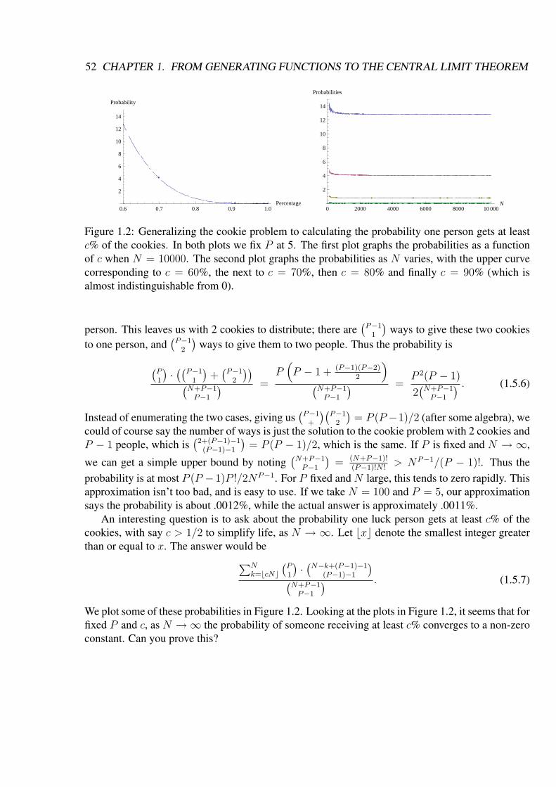
52 CHAPTER 1. FROM GENERATING FUNCTIONS TO THE CENTRAL LIMIT THEOREM
0.6 0.7 0.8 0.9 1.0Percentage
2
4
6
8
10
12
14
Probability
0 2000 4000 6000 8000 10 000N
2
4
6
8
10
12
14
Probabilities
Figure 1.2: Generalizing the cookie problem to calculating the probability one person gets at leastc% of the cookies. In both plots we fix P at 5. The first plot graphs the probabilities as a functionof c when N = 10000. The second plot graphs the probabilities as N varies, with the upper curvecorresponding to c = 60%, the next to c = 70%, then c = 80% and finally c = 90% (which isalmost indistinguishable from 0).
person. This leaves us with 2 cookies to distribute; there are(
P−11
)ways to give these two cookies
to one person, and(
P−12
)ways to give them to two people. Thus the probability is
(P1
) · ((P−11
)+
(P−1
2
))(
N+P−1P−1
) =P
(P − 1 + (P−1)(P−2)
2
)
(N+P−1
P−1
) =P 2(P − 1)
2(
N+P−1P−1
) . (1.5.6)
Instead of enumerating the two cases, giving us(
P−1+
)(P−1
2
)= P (P −1)/2 (after some algebra), we
could of course say the number of ways is just the solution to the cookie problem with 2 cookies andP − 1 people, which is
(2+(P−1)−1(P−1)−1
)= P (P − 1)/2, which is the same. If P is fixed and N → ∞,
we can get a simple upper bound by noting(
N+P−1P−1
)= (N+P−1)!
(P−1)!N !> NP−1/(P − 1)!. Thus the
probability is at most P (P − 1)P !/2NP−1. For P fixed and N large, this tends to zero rapidly. Thisapproximation isn’t too bad, and is easy to use. If we take N = 100 and P = 5, our approximationsays the probability is about .0012%, while the actual answer is approximately .0011%.
An interesting question is to ask about the probability one luck person gets at least c% of thecookies, with say c > 1/2 to simplify life, as N → ∞. Let bxc denote the smallest integer greaterthan or equal to x. The answer would be
∑Nk=bcNc
(P1
) · (N−k+(P−1)−1(P−1)−1
)(
N+P−1P−1
) . (1.5.7)
We plot some of these probabilities in Figure 1.2. Looking at the plots in Figure 1.2, it seems that forfixed P and c, as N →∞ the probability of someone receiving at least c% converges to a non-zeroconstant. Can you prove this?

1.5. GENERATING FUNCTIONS, COMBINATORICS AND NUMBER THEORY 53
How should we generalize the notion of a fair world? Let’s say there are N cookies and Ppeople, and for convenience let’s assume P divides N . Thus everyone should get exactly N/Pcookies. We would be surprised if everyone got exactly the fair amount; what isn’t immediatelyclear is how far below N/P someone must be before they cry foul. One natural way to solve this is tocompute not just the expected number of cookies someone receives, but also the standard deviation.We can do this with binary indicator variables. Let Xn be the random variable which is 1 if the firstperson receives cookie i and 0 otherwise. As there are P people, we see Xn = 1 with probability1/P and 0 with probability 1 − 1/P . Thus each Xi is a binomial random variable with parameterp = 1/P , and thus their expect values are p = 1/P and their variances are p(1− p) = (P − 1)/P 2.Letting X = X1 + · · ·+ XN , we have
E[X] =N∑
n=1
E[Xn] = N · 1
P=
N
P(1.5.8)
and
Var(X) =N∑
n=1
Var(Xn) = N · P − 1
P 2=
(P − 1)
P 2N. (1.5.9)
Thus the standard deviation is√
Var(X) =√
(P − 1)/P 2√
N .Perhaps a reasonable interpretation of making the world fair is that each person should be no
worse than one standard deviation below their expected number. What is the probability of thishappening if N is large and P is fixed? We now want each person to receive at least
m(N, P ) = bN/P −√
(P − 1)/P 2√
Nc (1.5.10)
cookies. Thus instead of solving
x1 + · · ·+ xP = N, xi ∈{
N
P+ m(N, P ),
N
P+ m(N,P ) + 1,
N
P+ m(N, P ) + 2, . . .
},
(1.5.11)as we did previously we make a change of variables by setting yi = xi −
(NP−m(N, P )
). This
leads us to solvingy1 + · · ·+ yP = Pm(N, P ), yi ∈ {0, 1, 2, . . . }. (1.5.12)
This is just the cookie problem with N − Pm(N,P ) cookies and P people. Thus the probabilityeveryone gets no worse than one standard deviation below their expected number of cookies is
(Pm(N,P )+P−1
P−1
)(
N+P−1P−1
) =
(P b√
(P−1)/P 2√
Nc+P−1
P−1
)(
N+P−1P−1
) . (1.5.13)
If we’re willing to accept a little more inequity, we can ask for the probability that each person getsno worse than N
P− km(N,P ) cookies (in other words, no one is more than k standard deviations
below their expected number). In Figure 1.3 we plot these probabilities for N varying from 1 to
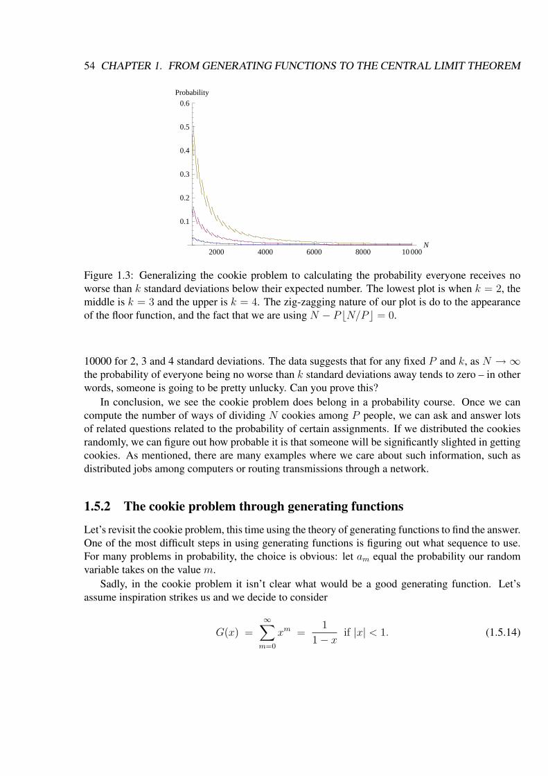
54 CHAPTER 1. FROM GENERATING FUNCTIONS TO THE CENTRAL LIMIT THEOREM
2000 4000 6000 8000 10 000N
0.1
0.2
0.3
0.4
0.5
0.6
Probability
Figure 1.3: Generalizing the cookie problem to calculating the probability everyone receives noworse than k standard deviations below their expected number. The lowest plot is when k = 2, themiddle is k = 3 and the upper is k = 4. The zig-zagging nature of our plot is do to the appearanceof the floor function, and the fact that we are using N − P bN/P c = 0.
10000 for 2, 3 and 4 standard deviations. The data suggests that for any fixed P and k, as N →∞the probability of everyone being no worse than k standard deviations away tends to zero – in otherwords, someone is going to be pretty unlucky. Can you prove this?
In conclusion, we see the cookie problem does belong in a probability course. Once we cancompute the number of ways of dividing N cookies among P people, we can ask and answer lotsof related questions related to the probability of certain assignments. If we distributed the cookiesrandomly, we can figure out how probable it is that someone will be significantly slighted in gettingcookies. As mentioned, there are many examples where we care about such information, such asdistributed jobs among computers or routing transmissions through a network.
1.5.2 The cookie problem through generating functions
Let’s revisit the cookie problem, this time using the theory of generating functions to find the answer.One of the most difficult steps in using generating functions is figuring out what sequence to use.For many problems in probability, the choice is obvious: let am equal the probability our randomvariable takes on the value m.
Sadly, in the cookie problem it isn’t clear what would be a good generating function. Let’sassume inspiration strikes us and we decide to consider
G(x) =∞∑
m=0
xm =1
1− xif |x| < 1. (1.5.14)
1.5. GENERATING FUNCTIONS, COMBINATORICS AND NUMBER THEORY 55
This is just the generating function of the sequence {am}∞m=0 with each am = 1. The generatingfunction can be simplified to G(x) = (1− x)−1 for |x| < 1 due to the geometric series formula.
We now show how this generating function solves the cookie problem, and then discuss how wecan generalize this to solve a variety of more difficult problems. Let r1,s(N) denote the number ofsolutions to m1 + · · · + ms = N where each mi is a non-negative integer. Note that r1,s(N) is justthe number of ways of dividing N cookies among s people (we switch to denoting the number ofpeople by s and not P as we’ll be differentiating with respect to this parameter in a moment); we’lldiscuss later why we choose to denote this as r1,s(N) and note rs(N). We claim
G(x)s =
( ∞∑m1=0
xm1
)· · ·
( ∞∑ms=0
xms
)=
∞∑N=0
r1,s(N)xN . (1.5.15)
For example, by direct multiplication we see that the first four terms of G(x)5 are 1 + 5x +15x2 + 35x3, and for N ∈ {0, 1, 2, 3} that the coefficient of xN in G(x)5 is
(N+5−1
5−1
). To prove
(1.5.15) for general s and N , we expand the product. We have terms such as xm1 · · · xms , which isxm1+···+ms = xN for some N . Assuming everything converges, when we expand the product weobtain xN many times, once for each choice of m1, . . . , ms that adds to N . Thus the coefficient ofxN in the expansion is r1,s(N). On the other hand, straightforward differentiation shows that
G(x)s =
(1
1− x
)s
=1
(s− 1)!
ds−1
dxs−1
1
1− x. (1.5.16)
Why do we want to write G(x)s like this? The reason is that we have a nice formula for G(x) asan infinite sum, and differentiating that s − 1 times is no problem. Note that we are using bothexpressions for G(x) (i.e., we’re using the infinite sum formulation as well as the geometric series’answer for what that sum is).
Substituting the geometric series expansion for 11−x
gives
G(x)s =1
(s− 1)!
ds−1
dxs−1
∞∑N=0
xN =∞∑
N=0
(N + s− 1
s− 1
)xN , (1.5.17)
which yields r1,s(N) =(
N+s−1s−1
). It is this second method of proof that we generalize. Below we
describe a variety of problems and show how to find their generating functions. In most cases, exactformulas such as (1.5.16) are unavailable; we develop sufficient machinery to analyze the generatingfunctions in a more general setting.
Exercise 1.5.4. With G(x) as in (1.5.14), show by direct multiplication that the first four terms ofG(x)5 are 1 + 5x + 15x2 + 35x3, and for N ≤ 3 that the coefficient of xN in G(x)5 is
(N+5−1
5−1
).
Exercise 1.5.5. Justify the arguments above. Show all series converge, and prove (1.5.16) and(1.5.17).

56 CHAPTER 1. FROM GENERATING FUNCTIONS TO THE CENTRAL LIMIT THEOREM
1.5.3 The generalized cookie problemFor the original cookie problem, we have a very nice combinatorial perspective that allows usto quickly and cleanly solve it. Let’s consider the following twist. We still have N cookiesand P people, but now each person wants to have a square number of cookies (the squares are{0, 1, 4, 9, 16, 25, . . . }). This is significantly harder, as we no longer have a combinatorial interpre-tation. How do we divide a number N into P squares? Let us know if you find a nice geometricway! Fortunately, there is a solution by using generating functions.
Let rk,s(N) denote the number of ways of writing N as a sum of exactly s integers, where eachinteger is a kthpower. In other words, it is the number of solutions to
x1 + · · ·+ xs = N, xi{0, 1, 2k, 3k, 4k, . . . } (1.5.18)
or equivalently it is the number of solutions to
zk1 + · · ·+ zk
s = N, zi ∈ {0, 1, 2, 3, 4, . . . }. (1.5.19)
We now see why we denoted the solution to the cookie problem r1,s(P ). The solution to the cookieproblem in §1.5.2, where we used generating function, immediately generalizes. We have our newgenerating function is
Gk(x) =∞∑
m=0
xmk
, (1.5.20)
and then
Gk(x)s =∞∑
N=0
rk,s(N)xn; (1.5.21)
unfortunately, if k 6= 1 we don’t have a simple formula for Gk(x). We don’t have an analogue ofthe geometric series formula to simplify this.
Sadly, this is a very common feature in mathematics. We can reduce the solution to a difficultproblem to a difficult sum or integral, which in general we cannot evaluate! All hope is not lost,however, as there are ways to approximate these sums and integrals. To describe these methods indetail is beyond the scope of this book, so we will content ourselves with a brief explanation andsome references to the literature. ADD REFS.
For technical reasons, it is often convenient to replace x with e2πit. This converts the problem toone of Fourier analysis. A major pain is the fact that we have infinitely many terms to sum, and thismeans there are convergence issues. We can fortunately bypass these difficulties with a very simplebut quite powerful observation. Let’s say we care about how many ways there are to write N as asum of exactly s numbers that are kthpowers; this is known as Waring’s problem. Clearly none ofthe numbers can exceed N1/k, so it suffices to look at the truncated generating series
Gk,N(x) =N1/k∑m=0
xmk
or Gk,N(t) =N1/k∑m=0
e2πimkt. (1.5.22)

1.5. GENERATING FUNCTIONS, COMBINATORICS AND NUMBER THEORY 57
We can pull off the solutions by integration. Using∫ 1
0
e2πiktdt =
{1 if k = 0
0 for k a non-zero integer(1.5.23)
(one can prove this using either complex analysis, or by writing eiθ as cos θ + i sin θ), we find
rk,s(N) =
∫ 1
0
Gk,N(t)e−2πiNtdt. (1.5.24)
While this is the solution to the problem, this is not an easy integral to evaluate! Fortunately thereare methods to approximate the function Gk,N(t), which allows us to approximate the integral.
This is just one of many problems that can be solved using this method. One of the most famousproblems in number theory is whether or not every ‘sufficiently large’ even number may be writtenas the sum of two primes (it is believed that ‘sufficiently large’ means ‘at least 4’). We show thatthe solution to this problem can be obtained by studying the generating function
GN(x) =∑p≤N
xp (1.5.25)
where p ranges over primes at most p, or equivalently using the generating function
GN(t) =∑p≤N
e2πipt. (1.5.26)
To see this, we compute GN(t)2, which is
GN(t)2 =∑p1≤N
e2πip1t∑p2≤N
e2πip2t =∑
p1,p2≤N
e2πi(p1+p2)t =2N∑n=4
a2,N(n)e2πint, (1.5.27)
where a2,N(n) is the number of ways of writing n as the sum of two primes each of which is at mostN . Thus we just need to pull off a2,N(N) to solve the problem. We can do this by integrating:
∫ 1
0
GN(t)2e−2πiNtdt =
∫ 1
0
N∑n=4
a2,N(n)e2πinte−2πiNt
=N∑
n=4
a2,N(n)
∫ 1
0
e2πi(n−N)tdt. (1.5.28)
The last integral is 1 if n = N and 0 otherwise, and thus the right hand side becomes a2,N(N).We have our answer:
a2,N(N) =
∫ 1
0
GN(t)2e−2πiNtdt; (1.5.29)
unfortunately we can’t analyze this integral well enough to solve the problem. We can computewhat we believe is the main term, but we cannot show that what is expected to be the error term issmaller. The situation is very different if we try to write N as the sum of three primes; there we canshow the error term is smaller, and prove that there are many ways of writing a large odd number asthe sum of three primes.