from micro to macro: a study of human brain structure ... · gergis shenouda, sherif dawood and...
TRANSCRIPT

From Micro to Macro: A Study of Human Brain Structure Based on Diffusion MRI and Neuronal Networks
BY
JOHNSON JONARIS GADELKARIM B.S., CAIRO University, EGYPT, 2004
M.S., University of Illinois at Chicago, Chicago, 2013
THESIS
Submitted as partial fulfillment of the requirements for the degree of Doctor of Philosophy in Electrical and Computer Engineering
in the Graduate College of the University of Illinois at Chicago, 2013
Chicago, Illinois
Defense Committee:
Dan Schonfeld, Chair & Advisor Alex Leow, Co-Advisor Richard Magin, Co-Advisor Anand Kumar, Psychiatry Natasha Devroye

ii
To my mother, Nawal, my wife Germaine, and my daughter Carla.

iii
ACKNOWLEDGMENTS
First, I would like to express my deep gratitude to my advisors, Dan Schonfeld, Alex Leow and
Richard Magin, for supervising my work and sharing their expertise during the past four years. I would also
like to thank Anand Kumar for having me in his research team and giving me the opportunity to work in the
prestigious and stimulating Psychiatric Institute. I am also extremely grateful to Natasha Devroye for her
participation in the committee. I would also like to thank Olusola Ajilore for reviewing my thesis and taking
the time to make insightful remarks and suggestions on my work.
Many people have contributed to the work presented in this thesis and I want to thank them here:
Olusola Ajilore, for introducing me to the field of Connectomics, Mark Meerschaert, for his valuable
mathematical inputs and for the long discussions about anomalous diffusion. Aifeng Zhang and Liang Zhan,
for helping me process the data, Shaolin Yang, for his help in the acquisition of the diffusion data, Carson
Ingo, for his useful comments on diffusion data processing. I also want to thank my collaborators: Jamie
Feusner, Donatello Arienzo, Paul Thomspon, Tom Barrick, Silvia Capuani, Marco Palombo, and Teena
Moody.
I will not forget all the friends I have made during these years: Ahmed Morsi, Bishoy Alphonse,
Gergis Shenouda, Sherif Dawood and family, Nasser Boshra and family, Reda Shaker and family, Maged
Saad and family, Samuel Botros and family, Fadel Azer and family, Sameh Soliman and family, and Mina
Khalil.
I would also like to thank my mother and brothers for all her efforts they made for me. Finally, I
would like to thank my wife, Germaine, for her love and support day-to-day during these years.
J.G.

iv
TABLE OF CONTENTS
CHAPTER PAGE
I. INTRODUCTION .................................................................................................................................. 1 1.1 Background ........................................................................................................................... 1 1.2 Thesis Organization ............................................................................................................... 3
II. THE HUMAN BRAIN .......................................................................................................................... 5 2.1 The Human Brain .................................................................................................................. 5 2.2 The White Matter .................................................................................................................. 9 2.3 Conclusion ............................................................................................................................. 11
III. BASIC PRINCIPLES OF DIFFUSION MRI ...................................................................................... 12 3.1 Introduction ........................................................................................................................... 12 3.2 Theory of Classical Diffusion ............................................................................................... 12 3.3 Nuclear Magnetic Resonance and Diffusion Magnetic Resonance Imaging ........................ 15 3.3.1 Pulse Gradient Spin Echo .......................................................................................................... 18 3.3.2 The Bloch-Torrey Equation ....................................................................................................... 21 3.3.3 Diffusion-Weighted Imaging and the Apparent Diffusion Coefficient ..................................... 24 3.3.4 Diffusion Tensor Imaging .......................................................................................................... 25 3.3.5 High Angular Resolution Diffusion Imaging ............................................................................. 29 3.3.5.1 Diffusion Spectrum Imaging ................................................................................................. 29 3.3.5.2 Single Shell HARD Imaging ................................................................................................. 31 3.3.5.2.1 Model-Based Approaches ..................................................................................................... 31 3.3.5.2.2 Model-Free Approaches ........................................................................................................ 34 3.4 Conclusion ............................................................................................................................. 35
IV. ANOMALOUS DIFFUSION .............................................................................................................. 37 4.1 Introduction ........................................................................................................................... 37 4.2 Continuous Time Random Walk model ................................................................................ 39 4.2.1 Long Jumps: Super Diffusion (Levy Flights): ........................................................................... 42 4.2.2 Long rests: Sub Diffusion: ......................................................................................................... 43 4.3 Anomalous Diffusion Magnetic Resonance Imaging ............................................................ 46 4.3.1 Isotropic Models ........................................................................................................................ 46 4.3.2 Anisotropic Models .................................................................................................................... 48 4.4 Conclusion ............................................................................................................................. 50
V. NEURONAL NETWORKS.................................................................................................................. 51 5.1 Introduction ........................................................................................................................... 51 5.2 Graph Theoretical Concepts for Network Analysis .............................................................. 52 5.3 Community Structure: A Literature Review ......................................................................... 58 5.3.1 Traditional Methods ................................................................................................................... 58 5.3.2 Hierarchical Clustering .............................................................................................................. 59 5.3.3 Divisive Algorithms ................................................................................................................... 59 5.3.4 Modularity Optimization ............................................................................................................ 60 5.3.3.1 Greedy Algorithms ................................................................................................................ 61 5.3.3.2 Simulated Annealing ............................................................................................................. 62 5.3.3.3 Spectral Optimization ............................................................................................................ 62 5.3.3.4 Limitations of Modularity ..................................................................................................... 63 5.4 Conclusion ............................................................................................................................. 64

v
TABLE OF CONTENTS (continued)
VI. ANISOTROPIC ANOMALOUS DIFFUSION MODELS ................................................................. 65 6.1 Introduction ........................................................................................................................... 65 6.2 Anisotropic Fractional Order Anomalous Diffusion Models ................................................ 65 6.2.1 Model I .................................................................................................................................. 65 6.2.1.1 Model I: Theory ..................................................................................................................... 66 6.2.1.2 Model I: Methods .................................................................................................................. 68 6.2.1.3 Model I: Results .................................................................................................................... 68 6.2.1.4 Model I: Discussion ............................................................................................................... 77 6.2.2 Model II ................................................................................................................................. 78 6.2.2.1 Model II: Theory ................................................................................................................... 79 6.2.2.1.1 Model II: Fractional Vector Calculus .................................................................................... 79 6.2.2.1.2 Model II: Multidimensional Fractional Diffusion Equation .................................................. 81 6.2.2.1.3 Model II: Fractional Order Bloch-Torrey Equation .............................................................. 82 6.2.2.2 Model II: Methods ................................................................................................................. 84 6.2.2.3 Model II: Results ................................................................................................................... 85 6.2.2.4 Model II: Discussion ............................................................................................................. 89 6.3 Discussion ............................................................................................................................. 92 6.4 Conclusion ............................................................................................................................. 93
VII. USING THE TENSOR DISTRIBUTION FUNCTION .................................................................... 94 7.1 Introduction ........................................................................................................................... 94 7.2 Background on Tractography ................................................................................................ 94 7.3 TDF-TRACT Tractography Algorithm ................................................................................. 97 7.4 Tractography Results ............................................................................................................. 100 7.4.1 Graphical User Interface for TDF-Tractography ................................................................... 100 7.4.2 Tractography of the Brain Stem and Cerebellar Peduncles ................................................... 100 7.4.3 Constructing the Dorsal Column-Medial Lemniscus (DCML) System ................................ 104 7.4.4 Constructing the Cortico-Spinal Tracts ................................................................................. 104 7.4.5 Constructing the Main Cerebellar Efferent Fibers ................................................................ 104 7.4.6 Constructing the Spinocerebellar and Rubrocerebellar Pathway .......................................... 105 7.4.7 Construction of the Cortico-Ponto-Cerebellar Pathway ........................................................ 105 7.5 Circular Standard Deviation .................................................................................................. 107 7.6 Conclusion ............................................................................................................................. 112
VIII. EXTRACTING THE BRAIN COMMUNITY STRUCTURES ...................................................... 113 8.1 Introduction ........................................................................................................................... 114 8.2 Methods ................................................................................................................................. 115 8.2.1 Constructing Brain Connectivity Network ............................................................................ 115 8.2.2 New Graph Metrics ............................................................................................................... 117 8.2.3 Path-Length Associated Community Estimation .................................................................. 118 8.2.3.1 Introducing ΨPL ..................................................................................................................... 118 8.2.3.2 Community Structure Estimation .......................................................................................... 118 8.2.3.3 Assessing group-level Community Structure Differences .................................................... 119 8.2.3.4 Statistical Analysis ................................................................................................................ 120 8.2.3.5 Testing for Frequency of Occurrence .................................................................................... 120 8.3 Results ................................................................................................................................... 121 8.3.1 Applying the New Graph Metrics to Bipolar Disorder ......................................................... 122 8.3.2 Comparison with Q Modularity............................................................................................. 124 8.3.3 Optimal Level of Hierarchical Reconstruction ...................................................................... 125 8.3.4 Community Structure Alterations in Bipolar Disorder .......................................................... 126

vi
TABLE OF CONTENTS (continued)
8.3.5 Community Structure Alterations in Depression Disorder .................................................... 130 8.4 Discussion ............................................................................................................................. 132 8.5 Conclusion ............................................................................................................................. 133
IX. CONCLUSIONS AND FUTURE RESEARCH ................................................................................. 134
APPENDICES ...................................................................................................................................... 136 Appendix A ........................................................................................................................... 137 Appendix B............................................................................................................................ 138 Appendix C............................................................................................................................ 139 Appendix D ........................................................................................................................... 140 Appendix E ............................................................................................................................ 150 Appendix F ............................................................................................................................ 152
CITED LITERATURE ......................................................................................................................... 166
VITA ..................................................................................................................................................... 175

vii
LIST OF TABLES
TABLE PAGE
I. MATHEMATICAL NOTATION USED IN THIS THESIS. ....................................................... 4
II. TIMELINE DESCRIBING THE HISTORY OF DIFFUSION MRI. .......................................... 18
III. MATHEMATICAL DEFINITIONS OF NETWORK METRICS. SHADING GROUPS METRICS OF SAME FAMILY. .................................................................................................................... 55
IV. MEAN AND STANDARD DEVIATION OF THE OBTAINED PARAMETERS USING THE MODEL IN EQUATION 6.8 AS WELL AS EIGENVALUES, FA AND MD ANALYSIS OF THE D AND Ψ TENSORS IN THE SELECTED ROIS HIGHLIGHTED IN FIGURE 21. ............... 76
V. MEAN AND STANDARD DEVIATION SUMMARY OF THE FITTED PARAMETERS AND THE COMPUTED METRICS ACROSS THE SLICE PRESENTED IN FIGURE 28 AND FIGURE 29................................................................................................................................................... 88
VI. INTER-HEMISPHERIC INTEGRATION ANALYSES IN THE FRONTAL, TEMPORAL, PARIETAL AND OCCIPITAL LOBES. THIS TABLE SHOWS THE MEAN AND STANDARD DEVIATION OF LOBAR INTER-HEMISPHERIC PATH LENGTH AND EFFICIENCY. ONLY GROUP DIFFERENCES REACHING STATISTICAL SIGNIFICANCE ARE SHOWN (BONFERRONI CORRECTION WITH A TOTAL OF 16 TESTS; CUT-OFF P VALUE 0.05/16=0.003) .............................................................................................................................. 123
VII. LIST OF NODES WHICH SHOWED SIGNIFICANT LOWER CONSISTENCY IN DEPRESSION RELATIVE TO HEALTHY CONTROLS AT P < 0.01 (UNCORRECTED). THE TABLE SHOWS MEAN AND STANDARD DEVIATION VALUES USING 2-SAMPLE T-TEST (FOR Ζ), AND THEIR CORRESPONDING P VALUES. ................................................................................... 130
VIII. SOME FUNCTIONS AND THE CORRESPONDING FOURIER DERIVATIVE .................... 143
IX. SOME FUNCTIONS AND THE CORRESPONDING LIOUVILLE DERIVATIVE ................ 145
X. SOME FUNCTIONS AND THE CORRESPONDING RIEMANN DERIVATIVE................... 146
XI. SOME FUNCTIONS AND THE CORRESPONDING LIOUVILLE-CAPUTO DERIVATIVE 146
XII. SOME FUNCTIONS AND THE CORRESPONDING CAPUTO DERIVATIVE ..................... 147
XIII. SOME FUNCTIONS AND THE CORRESPONDING CAPUTO DERIVATIVE ..................... 148
XIV. SOME FUNCTIONS AND THE CORRESPONDING CAPUTO DERIVATIVE ..................... 149
XV. LIST OF BRAIN REGIONS AS DEFINED BY THE FREESURFER SOFTWARE. ................ 150

viii
LIST OF FIGURES
FIGURE PAGE
1. Nerve cell ...................................................................................................................................... 6
2. Spinal gray and white matter cells, and a coronal slice of the human brain ................................. 7
3. The four lobes of the cerebral cortex and the cerebellum ............................................................. 8
4. The corpus callosum ..................................................................................................................... 10
5. The corticospinal tract. .................................................................................................................. 11
6. Diffusion of the molecules of dye in water ................................................................................... 13
7. Precession of the hydrogen atom in the presence of a magnetic field .......................................... 17
8. Schematic of the PGSE pulse sequence ........................................................................................ 21
9. Relaxation trajectory of the hydrogen atom .................................................................................. 23
10. Diffusion ellipsoid and water Brownian motion along the fibers ................................................. 28
11. Different anisotropy cases ............................................................................................................. 28
12. Metrics derived from the diffusion tensor ..................................................................................... 29
13. Diffusion orientation distribution function and the apparent diffusion coefficient profile ........... 30
14. Monoexponential estimate of the diffusion signal decay .............................................................. 38
15. A multi-scale look at neural tissue ................................................................................................ 39
16. Comparison of the trajectories of different diffusion schemes ..................................................... 45
17. Results of the fitted A and Γ tensors in the Hall and Barrick model ............................................ 49
18. Graph theoritic concepts ............................................................................................................... 55
19. The diffusion tensor elements of an axial slice through the optical tracts. ................................... 70
20. Selected regions of interest highlighted on the b0 image.............................................................. 71
21. Spatially resolved maps of the fitted parameters in Model I ......................................................... 72
22. The logarithm of the diagonal elements in Ψ ................................................................................ 73

ix
LIST OF FIGURES (continued)
23. Maps of the principal eigenvector and the largest eigenvalue of the Ψ and D tensors ................. 74
24. A colormap using the fractional order parameters and the diagonal unit preserving constants .... 75
25. Fitting curves to the stretched exponential model ......................................................................... 75
26. Relationship between laboratory frame, DTI, and analysis in Model II coordinate systems ........ 84
27. Spatially resolved maps of the unit preserving constants and the operational order parameters .. 86
28. Mean diffusivity, fractional anisotropy, mean anomalous exponent, and anomalous anisotropy 87
29. Contour plot of different versions of a 2D version of P(r, t) ........................................................ 91
30. Streamline tractography ................................................................................................................ 98
31. The GUI for the TDF-Tract program ............................................................................................ 102
32. The reconstructed tensor orientation distribution.......................................................................... 103
33. TDF-tractography results .............................................................................................................. 106
34. Visualization of multiple reconstructed fibers .............................................................................. 107
35. The averaged FADTI values (second panel) with respect to the geodesic distance ........................ 110
36. FATDF versus FADTI for both low and high resolution data ........................................................... 111
37. CSD and average FADTI plotted against the geodesic distance ..................................................... 112
38. Pipeline used to generate structural brain networks ...................................................................... 116
39. Community structure obtained for the Zachary club network ...................................................... 125
40. The average separability across .................................................................................................... 126
41. Binary trees showing mean community structures via the proposed metric ................................. 128
42. The frequencies at which several brain regions belong to the same community .......................... 129
43. Binary trees showing mean community structures via the proposed metric ................................. 131

x
LIST OF ABBREVIATIONS
3D
AAβ
AAL
ADC
AD
aFA
BOLD
CC
CC
CNS
CPC
CPL
CSD
CSF
CST
CTRW
DOT
DRTC
DSI
DT
DTI
DW
DWI
FA
3 dimensional
Anomalous Anisotropy
Automated Anatomical Labeling
Apparent Diffusion Coefficient
Anomalous Diffusion
Anomalous Fractional Anisotropy
Blood Oxygen Level Dependent
Corpus Callosum
Clustering Coefficient
Central Nervous System
Cortico-Ponto-Cerebellar
Characteristic Path Length
Circular Standard Deviation
Cerebral Spinal Fluid
Corticospinal Tract
Continuous Time Random Walk
Diffusion Orientation Transform
Dentate-Rubro-Thalamo-Cortical
Diffusion Spectrum Imaging
Diffusion Tensor
DT Imaging
Diffusion Weighted
DW Images
Fractional Anisotropy

xi
LIST OF ABBREVIATIONS (continued)
FACT
FDE
FID
FRT
gDTI
GM
HARDI
HOT
ICP
IID
NMR
NP
MAE
MCP
MRI
MSD
ODF
PAS
PDE
PDO
PGSE
PLACE
PNS
Fiber Assignment by Continuous Tracking
Fractional Diffusion Equation
Free Induction Decay
Funk-Radon Transform
Generalized DTI
Gray Matter
High Angular Resolution Diffusion Imaging
High Order Tensor
Inferior Cerebellar Peduncle
Identically Independent Distributed
Nuclear Magnetic Resonance
Non-deterministic Polynomial
Mean Anomalous Exponent
Middle Cerebellar Peduncle
Magnetic Resonance Imaging
Mean Squared Displacement
Orientation Distribution Function
Persistent Angular Structure
Partial Differential Equation
Probability Density Function
Pseudo-differential Operator
Pulse Gradient Spin Echo
Path Length Associated Community Estimation
Peripheral Nervous System

xii
LIST OF ABBREVIATIONS (continued)
QBI
QSI
RA
RF
ROI
SA
SCP
SH
SNR
STR
TDF
WM
Q-Ball Imaging
Q-Space Imaging
Relative Anisotropy
Radio Frequency
Region of Interest
Simulated Annealing
Superior Cerebellar Peduncle
Spherical Harmonics
Signal to Noise Ratio
Streamline Tracking
Tensor Distribution Function
White Matter

xiii
SUMMARY
A study on the human brain is carried out through the use of diffusion weighted magnetic resonance
imaging. The brain is studied at three different levels: micro, mid, and macro. At the micro-level, we utilize
the theory of continuous time random walk to describe the anomalous diffusive behavior of water molecules
in different brain tissues. This behavior is measured through multiple b-value diffusion weighted MRI
experiments. Two anisotropic models were derived through the introduction of fractional calculus into the
Bloch-Torrey equation. The obtained models are used to describe the complex structure of the brain white
and gray matter tissues through the introduction of new biometrics. The models allow the quantification of
the tortuosity and porosity of the brain tissues in different directions.
At the mid-level, a recent model, the tensor distribution function, is used to extract the brain white
matter fiber tracts. A new algorithm is designed to extract different complex fibers in the brain. The
algorithm is able to solve the fiber crossing problem at many locations. Moreover, a new metric is suggested
to measure fiber incoherence. The measure is then compared to the traditional metric, fractional anisotropy,
derived from the classical diffusion tensor model.
At the macro-level, the brain network community structure is studied. A new metric to extract the
modular structure of networks is derived. The metric is then applied on brain networks to extract the human
connectome community structure. Using the extracted connectome community structure, a framework is
designed to detect alterations on the nodal and modular levels occurring in group studies. The framework is
then applied on two datasets, bipolar and depression. Significant results were found in agreement with
previous clinical studies revealing the importance of the modular analysis of the human connectome.

1
I. INTRODUCTION
1.1 Background
The human brain is considered as being one of the most complex systems ever studied. Acquiring
information about the brain’s anatomy is a challenging task, extracting the neuronal architecture and
information about the brain while matter (WM) structure is even harder. Old methods have used dissection in
order to gain access to the WM (Dejerine and Dejerine-Klumpke 1895; Gray 1936). Nowadays, diffusion
weighted (DW) - magnetic resonance imaging (MRI) is considered as being the state of the art technique
capable of non-invasively extracting information about the brain’s WM structure. DW-MRI is based on the
diffusion of water molecules. The water diffusion is isotropic in mediums with no obstacles or walls. In
mediums with restricting walls and obstacles, such as the human brain WM, water molecules diffuses
anisotropically and tends to be restricted by the surrounding obstacles. Using DW-MRI measurements, we
are capable of describing the underlying structure of the brain WM. In this thesis, we are going to describe
the human brain on three levels: micro, mid and macro.
An important task in the analysis of the acquired DW-MRI measurements is the choice of a
mathematical model to describe the water diffusion. The very first model to be used in the mid 80’s (Le
Bihan et al. 1986) was a one dimensional Gaussian model. Then, a three dimensional (3D) Gaussian model
have been proposed by Basser et al. (Basser et al. 1993; Basser et al. 1994; Basser et al. 1994) and named
diffusion tensor imaging (DTI). This model has the capability of describing the main diffusion direction of
water. The model assumes a 3D Gaussian distribution for the average diffusion of water molecules. Despite
of its usefulness in describing many of the brain WM fibers pathways, it possesses a limitation manifested in
the limited capabilities of resolving crossing fibers. This limitation is mainly due to the low resolution of the
acquired DW-MRI signal. DW-MRI signal have a resolution between 1 to 8 mm3, while white matter fibers
have diameters below 30 µm (Poupon 1999). The existence of crossing fibers within the same voxel is then
inevitable. In fact, it is now estimated to be more than one third of the imaged voxels of the human brain WM
(Behrens et al. 2007). DTI limitations were the motivation to develop a family of techniques identified as

2
high angular resolution diffusion imaging (HARDI). In HARDI techniques, many DW signals are acquired
for the same voxel and a reconstruction model is chosen to extract the fibers directions at that voxel.
Diffusion is usually described by Fick’s second law which states that the rate of change of the
diffusing fluid concentration is directly proportional to its laplacian and the constant of proportionality is
called the diffusion coefficient D (mm2/s). In that framework, diffusion depends linearly on time. This type of
diffusion is called normal, Gaussian or Brownian diffusion which is previously used to model DTI. When
diffusion depends non-linearly on time, we call it anomalous diffusion (AD). AD is usually related to
diffusion in porous and complex mediums. DTI and HARDI assume that the water molecules diffusion in the
human brain belongs to the non-anomalous type. Recently, researchers started to exploit the anomaly of
diffusion in the human brain in order to obtain a better description of the fractal-like structure as well as the
porosity of the brain tissues. Simple isotropic models were introduced by Bennett et al. (Bennett et al. 2003)
and Magin et al. (Magin et al. 2008). Anisotropic models were also proposed by Hall & Barrick (Hall and
Barrick 2012), and De Santis et al. (De Santis et al. 2011). However, to date, the current anisotropic models
used to describe AD in the human brain do lack mathematical derivation and are presented as pragmatic
models. At the micro-level, we present in this thesis two 3D models based on the modification of the Bloch-
Torrey equation using fractional calculus. The models try to describe and quantify the complexity of the
human brain tissues. They introduce new biometrics and prove that the AD is anisotropic.
Extracting the brain WM fibers is called tractography. This process tries to reconstruct the brain
neural tracts as well as known fiber bundles and visualizes them using streamline tubes. At the mid-level, we
are going to exploit in this thesis a recently presented HARDI reconstruction method known as tensor
distribution function (TDF) (Leow et al. 2009) and use it for tractography. We are also going to study the
benefits of TDF over DTI by comparing the DTI-based anisotropy metric – fractional anisotropy (FA) – with
a newly TDF-based constructed one.
Tractography results can be used to extract the brain connectivity network which describes the
topological structure and connections between the different gray matter (GM) regions. The brain connectivity
network, also called connectome, was first introduced by Sporns et al. (Sporns et al. 2005). A brain structural
connectome consists of nodes which represent GM regions and edges connecting nodes which represent WM

3
fibers. Describing the brain as a network has allowed us to use many mathematical tools from the field of
graph theory to analyze it. One feature of brain networks is their “community structure” properties in which
nodes may be grouped into different communities. This property allows us to extract the topological
organization of the network and to partition it into a set of non-overlapping communities (also called modules
or clusters). At the macro-level, we present in this thesis a new framework to extract the different brain
communities and assess differences which might occur in neuropsychiatric diseases. The framework is
named “Path Length Associated Community Estimation” (PLACE) and it is based on a new quality function
introduced to assess the goodness of the extracted communities.
1.2 Thesis Organization
This thesis is organized in three parts. The first part includes this introduction and a brief description
of the human brain in chapter 2. The second part (chapters 3-5) covers briefly the physics of diffusion as well
as DW-MRI history and the different models used to describe normal diffusion in brain tissues (chapter 3). In
chapter 4, we introduce the physics of AD and its relation to DW-MRI. We state different models used to
describe AD in brain tissues. In chapter 5, we introduce the field of graph theory used to analyze brain
networks with an emphasis on community structure extraction techniques. In the last part (chapters 6-10), we
introduce the contributions of this thesis. First, in chapter 6, we present two new multi-dimensional fractional
order models for the Bloch-Torrey equation. We show that AD is anisotropic in brain tissues. Second, in
Chapter 7, we present the new tractography technique, and we introduce a new biomarker, the circular
standard deviation (CSD) which we use to proof the dependence of DTI-based FA metric on fiber
incoherence. Finally, in chapter 8, we present new graph metrics designed to measure the integration of left
and right hemispheres of the brain and its application on bipolar disorder. We also present the new
framework: PLACE which is validated through its application to brain networks extracted from bipolar
disorder and depression. Changes in communities were assessed and results were consistent with previous
clinical findings. Conclusions and future research are stated in chapter 10. Mathematical notations used in
this thesis are presented in Table I.

4
Table I: Mathematical notation used in this thesis.
x a scalar (italic) r a vector (bold italic) D a matrix (bold) r = (x y z)T a vector made out of 3 components: x y and z (.)T
transpose |x| absolute value of scalar x ||r|| Euclidian norm of a vector |D| determinant of a matrix D v.w scalar product of two vectors f(x) scalar valued function of a scalar f(x) scalar valued function of a vector f(x) vector valued function of a scalar f(x) vector valued function of a vector
d the space of d-tuples of reals 1{ ... }dx x ... dd∫ x the integration over multiple tuples:
1 2... ...d dx dx∫

5
II. THE HUMAN BRAIN
2.1 The Human Brain
The brain has been under extensive study for decades. It is part of the human nervous system and
plays the central role in that system. The human nervous system consists of two parts: the central nervous
system (CNS) which includes the brain and the spinal cord, and the peripheral nervous system (PNS) which
consists of a complex network of neural cells that connects the limbs and organs to the CNS. The brain is
responsible for the motor control, regulation and coordination of all our limbs and organs. It is also
responsible for the perception of the external world through the processing of sensory information. Moreover,
it also manages our abilities of reasoning, planning, decision-making and abstract-thought.
The main building block of the brain is the neuron (nerve cell) portrayed in Figure 1a. The neuron
receives signals from other neurons through input terminals called dendrites. Dendrites are thin extensions
that arise from the cell body, also called the soma, often extending for hundreds of micrometers and
branching multiple times. The neuron also emits signals to other neurons as electrochemical waves or pulses
travelling along thin fibers called axons. Axons are cable like structures covered by a dielectric material
called myelin which forms a layer around it, the myelin sheath. This layer increases the transmission speed of
electrical signals across the axon. A signal, when emitted, causes the release of chemicals called
neurotransmitters at the axon’s terminating point: synapse (Figure 1b). The synapse is a narrow space
between the neuron and other neurons or a muscle that can be seen as a communication end (Dayan and
Abbott 2001). It permits the neuron to send signals to another cell. A neuron can have over 1000 dendritic
branches and around 10000 synaptic connections with other neurons. There are about 80 to 100 billion
neurons in the human brain and 100 trillion synapses; they form a complex network of connections
(Herculano-Houzel 2009).

6
Figure 1: a) Nerve cell, b) Electrical signal propagating to the next cell through the axon and dendrites, notice the chemical reaction at the synapse. Both figures were adapted from Wikipedia.
On a larger scale, the human brain is made out of several elements. The cerebrospinal fluid (CSF)
surrounds the brain and exists also in the ventricle system which is shown in Figure 2. It acts as a “cushion”
providing the necessary mechanical and immunological protection. The brain is made out of two main types
of tissues: the gray and white matters (Figure 2). The WM consists of the neuron axons. Bundles of axons are
called fiber tracts. The GM is made out of the neuronal cell bodies and is full of capillary blood vessels
which give it the gray-brown color. Globally, we can consider that the WM acts as a network of cables which
interconnects the different regions of the GM.
On a macroscopic scale, the brain consists of three major parts: the cerebrum, the cerebellum and the
brain stem shown in Figure 3. The cerebrum is made out of the two cerebral hemispheres separated by the
central fissure and interconnected through a dense bundle of WM fibers called the corpus callosum (CC). The
two hemispheres form the largest part of the human brain. The outer shell of the cerebrum, also called the
cerebral cortex, is made out of highly folded GM tissues, the folding helps to increase the surface area in the

7
limited volume of the human skull. The cortex contains regions responsible for sensory, control of voluntary
movement, speech and cognition functions.
Figure 2: Spinal gray and white matter cells. Red arrows point to GM containing neuron cell bodies. WM contains cell axons, adapted from neuro-histology Atlas: http://vanat.cvm.umn.edu/neurHistAtls/ (left). A coronal slice of the human brain, we can see the designation of the enumerated divisions is as follows: 1) Cerebrum, 2) Thalamus, 3) Midbrain, 4) Pons, 5) Medulla oblongata, 6) Spinal cord. The black regions above number two contain CSF in a living brain, they are called ventricles, adapted from Wikipedia (right).

8
Figure 3: (a) the four lobes of the cerebral cortex and the cerebellum, adapted from (Gray 1936), (b) midsagittal cut of the human brain showing the cerebral cortex, the cerebellum and the brain stem, adapted from Wikipedia.
We can divide each of the two cerebral hemispheres cortexes into four lobes (Figure 3a). 1) The
frontal lobe (blue region in Figure 3a) responsible for motor control, speech and memory functions. It also
controls planning, reasoning and decision making actions. 2) The temporal lobe (green region in Figure 3a)
manages the processing of audio-visual information as well as language comprehension. 3) The parietal lobe
(yellow region in Figure 3a) integrates visual and other sensory information in order to control spatial
orientation as well as arm and eyes movement. 4) Finally, the occipital lobe (red region in Figure 3a) which
handles the primary visual processing functions.
The cerebellum (Figure 3), also called little brain, handles quick responses to sensory signals and
equilibrium functions. It contributes to coordination, precision and accurate timing of movements. In other
words, it acts as a fine tuning center for motor functions. It receives inputs through the spinal cord and other
parts of the brain. The brain stem (Figure 3b) consists of three parts, first the medulla oblongata which
controls involuntary functions such as heart rate and breathing. Second, the midbrain which is associated
with visual reflexes control, sleep and wake, alertness and temperature regulation functions. Finally, the

9
pons, also called the bridge, consists of WM tracts which interconnect the cerebrum to the cerebellum and
medulla.
This thesis tries to investigate three main aspects of the brain. First, on the micro level, we try to
describe the porosity of the brain tissues using the theory of AD by proposing two different anisotropic
models in chapter 6. Second, on the macro level, we try to reconstruct fiber tracts using the proposed
tractography method in chapter 7. Finally, on a global level, we try to extract the underlying organizational
structure, also called community structure, of the different cortical regions. We also detect alterations in that
structure which might occur due to neuropsychological diseases. This is presented in chapter 8.
2.2 The White Matter
As mentioned above, the WM consists of the different fiber bundles. In this section we will describe
the most important bundles which might be mentioned in this thesis. There are three types of fibers: 1)
commissural fibers which interconnect the two cerebral hemispheres, 2) association tracts which interconnect
the different lobes within the same hemisphere, and 3) projection fibers which interconnect the spinal cord,
cerebellum and subcortical structures. We will present two main fiber bundles: the corpus callosum and the
corticospinal tract.
Corpus Callosum
The CC, also known as the colossal commissure, is the largest and densest fibers bundle in the brain
made out of about 250 million axons. It interconnects the two cerebral hemispheres. It can be considered as a
flat bundle of fibers which lies beneath the cortex. The CC can be divided into four parts from anterior to
posterior: rostrum, genu, body and splenium (Figure 4). We can see that the CC fibers are spread in the
various parts of the cerebral cortex. Curving fibers at the genu are called forceps minor while fibers which
curve at the splenium are called forceps major (Figure 4-right).

10
Figure 4: The corpus callosum. In the left, a sagittal cut showing the different divisions of the CC. In the right, a transverse cut showing the CC fibers interconnecting the two cerebral hemispheres. Figures adapted from Wikipedia.
Corticospinal Tract
The Corticospinal Tract (CST) fiber bundle runs vertically from the spinal cord to the brain. The
CST contains mostly motor related tracts. Figure 5 shows the CST and how it fans out into different regions
in the cerebral cortex.

11
Figure 5: The corticospinal tract, adapted from (Gray 1936).
2.3 Conclusion
In this chapter, we have presented a basic description of the human brain anatomy which will be
needed to understand the rest of this thesis. In the next chapter, we will introduce diffusion MRI as well as
the necessary basics from physics.

12
III. BASIC PRINCIPLES OF DIFFUSION MRI
3.1 Introduction
DW-MRI is considered a recent technology invented in the past three decades. It is a noninvasive
modality of MRI which allows us to do in-vivo analysis on fibrous tissues such as the brain WM and skeletal
muscles such as the heart. It is based on the diffusion transport phenomena of gas and fluids. Several
applications have emerged from the inspection of the DW imaging data. The most famous one is the early
diagnosis of stroke. Post-processing of diffusion data have allowed us to reconstruct the brain WM fibers, the
process known as tractography. Tractography has helped in charting the brain network and have deepened
our understanding on the organizational structure of the human brain. In this chapter, we review the basic
physics of diffusion. Then, we present different models used to describe the DW-MRI measurements of the
water molecules in WM tissues. This chapter was inspired from review articles and chapters from (Le Bihan
et al. 2001; Tuch 2002; Le Bihan 2003; Descoteaux 2008) which I found as great sources for the basic
concepts of the diffusion MRI field.
3.2 Theory of Classical Diffusion
Gas and fluid diffusion is a transport phenomenon discovered by the botanist Robert Brown in 1827.
Brown has observed the motion of pollen particles in water. He initially thought that the motion exists
because the pollens are alive. Repeating his experiment with dust particles has revealed a jittery kind of
motion. However, the pollens were not moving because they were alive. In fact, it was due to random
collisions happening between water molecules. This was later identified as the diffusion phenomena or the
Brownian motion. Figure 6 shows the diffusion of the molecules of dye in water. Notice that the dye
molecules move from the higher concentration region to the lower concentration region. It is important to
mention that diffusion will even occur in thermodynamic equilibrium state (constant temperature and
pressure).

13
Figure 6: Diffusion of the molecules of dye in water, the dye molecules move from the higher concentration region to the lower concentration region. Notice that even at thermodynamic equilibrium state (last stage); the water molecules are still in a continuous motion across the membrane. Figure adapted from Wikipedia.
In 1855, Fick modeled diffusion as a differential equation (Fick 1855). Fick’s first law states that: the
net particle flux, J(r), is related to the particle concentration, 𝐶(𝒓, 𝜁), at position r and timeτ through the
following equation:
𝐽(𝒓) = −𝐷∇𝐶(𝒓, 𝜁) (3.1)
where D is the self-diffusion coefficient of units mm2/sec. The ∇ sign is the gradient taken w.r.t. position. The
negative sign indicates that particles flow from higher concentration region to lower concentration region.
The diffusion coefficient depends on the size of the diffusing molecules, temperature and environment.
Assuming an isotropic diffusion (same diffusion in all directions) enforces D to be a scalar. Using the law of
conservation of mass at the crossing membrane, 𝜕𝐶(𝒓,𝜁)𝜕𝑡
= −∇𝐽(𝒓), and substituting in equation 3.1, we get:
𝜕𝐶(𝒓, 𝜁)𝜕𝑡
= 𝐷∇2𝐶(𝒓, 𝜁) (3.2)
This is called Fick’s second law which predicts how diffusion causes the concentration to change with time.
In anisotropic mediums, where the diffusion is constrained in some directions and free in the others, for

14
example in biological tissues where cell membranes form walls, one can replace D by the diffusion tensor
(DT) D. The DT is a symmetric positive definite matrix and can be written as:
𝐃 = �
𝐷𝑥𝑥 𝐷𝑥𝑦 𝐷𝑥𝑧𝐷𝑥𝑦 𝐷𝑦𝑦 𝐷𝑦𝑧𝐷𝑥𝑧 𝐷𝑦𝑧 𝐷𝑧𝑧
� (3.3)
Hence, equation 3.2 can be then generalized in the form:
𝜕𝐶(𝒓, 𝜁)𝜕𝑡
= ∇𝑇𝐃∇𝐶(𝒓, 𝜁) (3.4)
where [.]T represents transpose. In 1905, Einstein re-described diffusion in a statistical framework in the
context of a random walk scenario (Einstein and Fürth 1956). He hypothesized that if one could observe the
movement of a single molecule in a fluid, one could observe a random trajectory of motion. Furthermore, this
trajectory is independent of neighboring molecules motion trajectories. However, one cannot describe
trajectories for all molecules. So, Einstein suggested the following: on a macro scale, if the number of
molecules is large and they have the freedom to diffuse anywhere, one could characterize their mean squared
displacement (MSD) from a starting point over a timeτ. He then described diffusion by a probability density
function (PDF), P(r,τ), which represents the probability of finding a particle at location r and at timeτ. This
PDF is currently known by the name of diffusion propagator. Einstein proved that the MSD averaged over
all diffusing molecules in an isotropic medium is proportional to the diffusing time τ and the constant of
proportionality is the self-diffusion coefficient D. He expressed this in the form:
⟨𝒓𝑻𝒓⟩ = 6𝐷τ (3.5)
where <.> denotes the ensemble average and r is the net displacement position vector: r = rτ – r0 with r0 is the
original position of a particle and rτ is the position after timeτ. Einstein has reached equation 3.2 with the
particle concentration 𝐶(𝒓, 𝜁) replaced by the diffusion PDF. In current literature discussing diffusion, the
propagator usually replaces C(r,ζ) in equations 3.1 to 3.4. His equation can be generalized to the DT model
similar to equation 3.3. Experimentally, one could measure the value of D for water at a temperature of 30°C

15
to be 2.6 X 10⁻³ mm2/s. In other words, in 1 ms, water molecules will move, on average, 4 µm in all
directions. The general solution of the DT model is a Gaussian distribution given by:
𝑃(𝒓, τ) =1
�(4𝜋|𝐃|𝜏)3exp �−
14𝜏𝒓𝑇𝐃−1𝒓� (3.6)
where |𝐃| is the determinant of the DT. In that context, D can be considered as the covariance matrix of the
3-variate Gaussian diffusion propagator describing the motion of the diffusing molecules. In isotropic
mediums when D is a scalar, we can write:
𝑃(𝒓, τ) =
1
�(4𝜋𝐷𝜏)3exp�−
‖𝒓‖2
4𝐷𝜏 � (3.7)
where ‖. ‖ is the norm. Further analysis of the DT model will be discussed later in this chapter when
discussing the DTI model. From above, one could notice that D is a scalar constant which makes us to
wonder about how this can be used to describe different tissues in DW-MRI. In fact, due to the presence of
obstacles such as cell membranes and macromolecules, biological tissues do possess a hindering nature
which will lower the values of the measured D. In this case, the measured D in DW-MRI is called the
apparent diffusion coefficient (ADC) (Le Bihan et al. 1986). We now start describing how we do actually
measure the ADC.
3.3 Nuclear Magnetic Resonance and Diffusion Magnetic Resonance Imaging
We will start by presenting a brief history about MRI. Before MRI and DW-MRI, people have
measured diffusion using nuclear magnetic resonance (NMR) spectroscopy. NMR spectroscopy is a method
by which one can use the magnetic properties of atoms in order to determine their physical and chemical
properties. It is based on the phenomenon of NMR first discovered in 1938 by Isidor Rabi et al. (Rabi et al.
1992) who won the Nobel Prize in Physics in 1944 for this work. In 1946, Felix Bloch (Bloch 1946) and
Edward Mills Purcell (Purcell et al. 1946) simultaneously presented a new expansion for Rabi’s technique to
be used on gas and liquid. They both won the Nobel Prize in Physics in 1956 for their discovery. Rabi, Bloch
and Purcell hypothesized that in the presence of a strong homogenous magnetic field, hydrogen atoms, 1H,

16
will precess around the same axis of the applied magnetic field at a specific frequency, also called the
Larmor frequency, which characterizes the hydrogen atom and depends on the applied field strength (Figure
7a). This state was then called equilibrium. They noticed that a perturbation to this state using a radio
frequency (RF) pulse could be absorbed by the atom only if its frequency matched the Larmor frequency.
This was called the resonance state of the atom shown in Figure 7b. The RF pulse is usually called a 90
degree pulse because it tips the hydrogen atom in the transverse plane perpendicular to the applied magnetic
field (Figure 7b). After the end of the RF pulse, an oscillatory damped signal is emitted from the ensemble of
hydrogen atoms in resonance, this signal is characterized by the Larmor frequency and is called the free
induction decay (FID) shown in Figure 7c.
In 1973, Paul Lauterbur designed a technique to generate 2D MR images which made him won the
Nobel Prize in Physiology and Medicine jointly with Peter Mansfield in 2003. In 1950, Hahn introduced
spin-echo to NMR. He suggested a technique to rebuild the damped FID signal by applying another RF pulse
for twice the duration of the 90 degree pulse following to the application of the initial 90 degree pulse (Hahn
1950). He observed that the emitted signal by the hydrogen builds-up after a certain period (Figure 7d). This
was a very essential step in the development of DW-MRI. In 1956, Torrey have introduced a new term in the
Bloch equation to account for diffusion (Torrey 1956). Using the spin-echo pulse sequence, Edward Stejskal
and John Tanner have developped in 1965 the pulse gradient spin-echo (PGSE) sequence which allows the
measurement of the ADC (Stejskal and Tanner 1965). In the next section, we are going to discuss the PGSE
in more details. Table II shows a timeline which describes briefly the diffusion MRI history.

17
Figure 7: a) Precession of the hydrogen atom (proton) in the presence of a magnetic field B, red and green colors represent positive and negative polarities respectively, b) The application of a 90 degree tipping RF pulse will cause the hydrogen atom to precess in the transverse plane perpendicular to the main applied magnetic field, c) Free induction decay, notice that the signal exhibits a damping oscillatory behavior, d) Spin-echo pulse sequence, notice how the echo signal builds-up after the 180 degree pulse. Figure adapted from Wikipedia.

18
Table II: Timeline describing the history of diffusion MRI.
1938 1946 1950 1956 1965 1973 1985 1990-1991 1992
Isidor Rabi
Felix Bloch
Edward Purcell
Erwin Hahn
H.C.
Torrey
Edward Stejskal
&
John Tanner
Paul Lauterbur
Taylor & Bushell
Denis Le Bihan
& Breton
Maichel Moseley
et al.,
Douek et al.
Peter Basser
et al.
Principles of NMR Spin-echo
Diffusion in NMR
PGSE 2D MRI Scalar DW-MRI, ADC and Trace
Imaging DTI
3.3.1 Pulse Gradient Spin Echo
In 1965, Stejskal and Tanner have designed the pulsed gradient spin echo (PGSE) sequence in order
to acquire information about the diffusion of particles (Stejskal and Tanner, 1965). Before discussing the
PGSE sequence, we would like to present the notion of a gradient. From the previous discussion, we recall
the dependence of the hydrogen atoms precessional frequency on the strength of the applied magnetic field.
This fact describes what is known to be the Larmor equation which states that the precessional frequency of
the hydrogen atom is directly proportial to the applied magnetic field and the constant of proportionality is
called the gyromagnetic ratio, γ, a unique characteristic for every element, and have units of rad/sec/Tesla.
The application of a linearly space-varying magnetic field, i.e. a gradient, imposed on the originally applied

19
strong static magnetic field, will cause a position dependence for the hydrogen atoms precessional frequency.
In other words, each atom will precess at a different frequency according to the strength of the magnetic field
present at its location which will cause each atom to gain a different phase along time. Applying the gradient
field for a period of time will create a gradient of phase over the volume under study. This phase gradient can
be reversed by the application of a 180 degree RF pulse followed by a gradient with exactly the same
amplitude, duration and polarity.
Since water consists of two hydrogen atoms, one can apply NMR principles to a water specimen. The
PGSE pulse sesquence illustrated in Figure 8 can be used to measure the diffusion of water molecules at a
specific direction g (a unit vector). By default a strong magnetic field B is applied on the speciemen to allow
the exploitation of its NMR properties. The PGSE consists of four steps. First, a 90 degree pulse is applied
which will tip all the atoms in the transverse plane, recall Figure 7b. Seond, a dephasing gradient is then
applied in direction g with strength G and duration δ will cause a phase gradient to buil-up across the
specimen. Third, a 180 degree RF pulse is applied. Finally, we apply a second rephasing gradient in direction
g with the same amplitude and duration – as the first gradient – after a time Δ from the first gradient. In the
absence of the water molecules displacement, the second rephasing gradient should cancels the phase shift of
the static molecules. However, under the random walk of water molecules, i.e. diffusion, a distribution of
phase occurs due to the displacement of different molecules. This distribution will cause a loss in the signal
coherence which can be observed as a loss of the spin-echo signal amplitude when compard to the no-
diffusion experiment. Please note that the applied gradient pulses were assumed to be short enough so that
the water diffusion is negligible during that time (δ).
In their 1965 paper, Stejskal and Tanner have showed that the acquired NMR signal, S(q,τ), in the
PGSE experiment is the 3D Fourier transform, ℱ, of the diffusion propagator PDF, P(r,τ), mentioned in
section 3.2. Assuming an initial delta distribution of material at r = 0 and τ = 0+, (i.e. P(r = 0,τ) = δ(r)), we
can write:

20
𝑆(𝒒, 𝜏)𝑆0
= � 𝑃(𝒓, τ) exp(−𝑖2𝜋𝒒𝑇𝒓)ℝ3
𝑑𝒓 = ℱ{𝑃(𝒓, τ)} (3.8)
where the value of q is given by q = γδGg/2π, with γ being the nuclear gyromagnetic ratio for water protons,
G is the applied gradient amplitude and g is a unit vector in its direction, S0 is the baseline image acquired
without any diffusion gradients (also called b = 0 image). In diffusion MRI, we seek out the reconstruction of
the diffusion propagator PDF. An exhaustive model-free solution is to sample all possible q vectors or the so-
called q-space which have been realised in q-space imaging (Callaghan, 1991). A simple solution is to
assume that the propagator takes the form of a Gaussian distribution. In that case, equation 3.8 could be
worked out analytically and one could reach the follwing equation:
𝑆(𝒈, 𝜏 ) = 𝑆0 exp(−𝜏‖𝒒‖2𝐷𝒈𝑇𝒈) = 𝑆0 exp(−𝑏. ADC) (3.9)
where b is called the b-value given by 𝑏 = τ ‖𝒒‖2 with units of s/mm2 and was first introduced by Le Bihan
et al. (Le Bihan et al. 1986) and the ADC is the apparent diffusion coefficient. From the above equation, we
can see that increasing the b-value will decrease the amplitude of the acquired signal, thus decreasing the
signal to noise ratio (SNR). Notice that D here is scalar since the measurement was assumed to be in only one
direction which assumes an isotropic medium under test. In anisotropic mediums, the DT D could be used
instead. In the next section we will try to obtain equation 3.9 using a different approach starting from the
Bloch-Torrey equation (Torrey 1956).
21
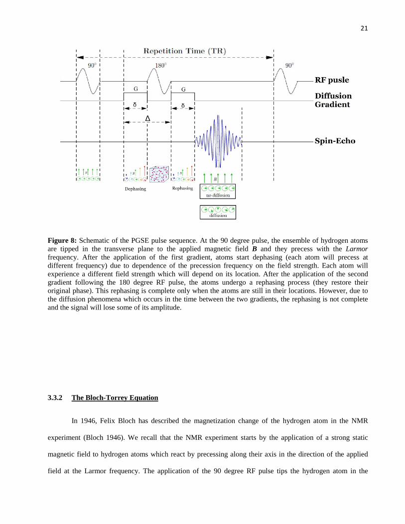
Figure 8: Schematic of the PGSE pulse sequence. At the 90 degree pulse, the ensemble of hydrogen atoms are tipped in the transverse plane to the applied magnetic field B and they precess with the Larmor frequency. After the application of the first gradient, atoms start dephasing (each atom will precess at different frequency) due to dependence of the precession frequency on the field strength. Each atom will experience a different field strength which will depend on its location. After the application of the second gradient following the 180 degree RF pulse, the atoms undergo a rephasing process (they restore their original phase). This rephasing is complete only when the atoms are still in their locations. However, due to the diffusion phenomena which occurs in the time between the two gradients, the rephasing is not complete and the signal will lose some of its amplitude.
3.3.2 The Bloch-Torrey Equation
In 1946, Felix Bloch has described the magnetization change of the hydrogen atom in the NMR
experiment (Bloch 1946). We recall that the NMR experiment starts by the application of a strong static
magnetic field to hydrogen atoms which react by precessing along their axis in the direction of the applied
field at the Larmor frequency. The application of the 90 degree RF pulse tips the hydrogen atom in the

22
transverse plane (Figure 7b). The atom, however, recovers its orientation in the direction of the applied
magnetic field (the equilibrium state), we call this: relaxation (Figure 9). There are two types of relaxation in
the NMR experiment: 1) T1-relaxation, also called spin-lattice relaxation, where the hydrogen atoms give
back the absorbed energy from the RF pulse to the surrounding environment or lattice. 2) T2-relaxation, also
called spin-spin relaxation, where the hydrogen atoms start dephasing due to the energy exchange between
them. Both relaxation types will cause the measured net magnetization (the detected signal) in the transverse
plane to decay. The net magnetization of an ensemble of atoms in a specimen can be detected by means of
coils surrounding it as shown in Figure 9.
The Bloch equation describes the decay of the transverse net magnetization moment M as a function
of the T1 and T2 relaxation times. The Bloch equation states:
𝑑𝑴𝑑𝑡
= 𝑴 × 𝛾𝑩�����Precession
−𝑀𝑥𝒊 + 𝑀𝑦𝒋
𝑇2�������spin−spin relaxation
−(𝑀𝑧 −𝑀0)𝒌
𝑇1���������spin−latticerelaxation
(3.10)
where M = [Mx My Mz]T is the net magnetization moment of the ensemble of hydrogen atoms in the specimen,
B = [0 0 B0]T is the static magnetic field and it is assumed to act in the z direction, i, j and k are unit vectors
in the x, y and z directions. The first part of the equation describes the precessional effect due to the applied
static magnetic field. The second and third parts describe the effect of the T1 and T2 relaxations.

23
Figure 9: Relaxation trajectory of the hydrogen atoms in a specimen present in a static magnetic field B0 after the end of the RF excitatory pulse. The net magnetization M is detected by means of horizontal coils. The atoms return to the equilibrium state where they are oriented parallel to the applied static field.
In 1956, Henry Torrey introduced a diffusion term in equation 3.10 (Torrey 1956). Ignoring the T1
and T2 relaxation and considering only the transverse magnetization Mxy to be the combination of Mx and My
in the form: Mxy = Mx + iMy where i =√−1, he wrote:
𝜕𝑀𝑥𝑦
𝜕𝑡= −𝑖𝛾(𝒓.𝑮)𝑀𝑥𝑦 + ∇T𝐃∇𝑀𝑥𝑦 (3.11)
where r = [x y z]T is a position vector, G = [Gx Gy Gz]T is the applied gradient in the PGSE sequence, ∇=
� 𝜕𝜕𝑥
𝜕𝜕𝑦
𝜕𝜕𝑧�𝑇and D same as equation 3.3. Equation 3.11 is known as the Bloch-Torrey equation. Using the
method of separation of variables, a solution of the following form can be assumed:
𝑀𝑥𝑦(𝒓, 𝑡) = 𝐴(𝑡)exp (−𝑖𝛾 𝒓.𝑭(𝑡)) (3.12)

24
where 𝑭(𝑡) = ∫ 𝑮(𝑡′)𝑑𝑡′𝑡0 . Substituting 3.12 in 3.11 and noting that
∇ exp�−iγ𝐫.𝐅(t)� = −𝑖𝛾𝑭(𝑡) exp�−iγ𝐫.𝐅(t)� we obtain:
𝜕[𝐴(𝑡)]𝜕𝑡
= −𝛾2�𝑭(𝑡)𝑇𝐃𝑭(𝑡)�𝐴(𝑡) (3.13)
Integrating, we get:
𝐴(𝑡) = 𝐴0 exp �−𝛾2 � 𝑭(𝑡′)𝑇𝐃𝑭(𝑡′)𝑑𝑡′
𝑡
0� (3.14)
Hence, one can write:
𝑀𝑥𝑦 = 𝑀0 exp�−𝛾2 � 𝑭(𝑡′)𝑇𝐃𝑭(𝑡′)𝑑𝑡′
𝑡
0� (3.15)
Performing the integration on the PGSE pulse using square gradients, we get:
𝑀𝑥𝑦 = 𝑀0 exp �−(𝛾𝛿‖𝑮‖)2�Δ − 𝛿3� �𝒈𝑇𝐃𝒈�
= 𝑀0 exp(−𝑏𝒈𝑇𝐃𝒈) (3.16)
where 𝒈 = 𝑮‖𝑮‖
, 𝑏 = (𝛾𝛿‖𝑮‖)2�Δ − 𝛿3� � is the b-value mentioned in section 3.3.1 computed for the PGSE
sequence. In light of equation 3.16, we can describe the acquired diffusion signal in the form:
𝑆(𝒈, 𝑡) = 𝑆0 exp(−𝑏𝒈𝑇𝐃𝒈) (3.17)
where S0 is the signal acquired at b = 0. The last equation describes the DT model applied in anisotropic
mediums. In isotropic mediums, a scalar diffusion coefficient will be used and we will reach equation 3.9.
Equation 3.19 is considered to be the basis of the DTI model.
3.3.3 Diffusion-Weighted Imaging and the Apparent Diffusion Coefficient
The beginnings of diffusion MRI dates back to 1985 when Taylor and Bushell acquired the first DW
images (DWI) of a small hen’s egg (Taylor and Bushell 1985). The images were the acquired data of the

25
applied PGSE pulse sequence in one gradient direction. In the next year, Le Bihan et al. presented the first in-
vivo DWI acquisition of a human brain (Le Bihan et al. 1986). In that study, he introduced the notion of the
b-value and provided the formulation to compute the ADC from the acquired DWI using equation 3.9 with b
computed for the PGSE sequence as in 3.16. Two acquisitions were needed: one with no diffusion, also
called b0 image, and another one with the PGSE applied. He noted changes in ADC in different tissues in the
brain. He has also observed that GM tissues possess a higher ADC compared to WM tissues. However, both
tissue types had an ADC lower than the self-diffusion coefficient of water. The ADC of CSF was found to
vary according to location. In general, it has a value close to the self-diffusion coefficient of water and it was
significantly higher in the ventricles.
The usage of different gradient directions appeared in 1990 when Moseley et al. measured the ADC
along the x and z axis in a cat brain (Moseley et al. 1990). At that time, it became clear that diffusion in
biological tissues is anisotropic. Moseley et al. suggested the ratio ADCz/ADCx to characterize the level of
anisotropy in tissues and it was called the anisotropy index. Unfortunately, this metric was rotationally
variant and it depended on the gradient direction used in the PGSE sequence. In the next section we will
introduce the DTI model which is rotationally invariant.
3.3.4 Diffusion Tensor Imaging
Many of the fibrous biological tissues such as the heart muscle and the brain WM exhibit anisotropic
water diffusion. Basser et al. have proposed the DT model (equation 3.6) to describe the diffusion propagator
PDF (Basser et al. 1993; Basser et al. 1994; Basser et al. 1994). In that case, equation 3.17 is used to describe
the acquired diffusion signal. From equation 3.3, we can see that the DT, D, is made out of 6 unknowns
(since it is symmetric). Hence, we need to acquire at least 6 DWI in 6 non-collinear gradient directions in
addition to the b0 image (S0) to be able to compute the DT. A system of linear equations can then be formed
by rewriting equation 3.17 in the form:
−1𝑏 log �
𝑆(𝒈, 𝑡)𝑆0
� = 𝑔𝑥2𝐷𝑥𝑥 + 𝑔𝑦2𝐷𝑦𝑦 + 𝑔𝑧2𝐷𝑧𝑧 + 2𝑔𝑥𝑔𝑦𝐷𝑥𝑦 + 2𝑔𝑥𝑔𝑧𝐷𝑥𝑧 + 2𝑔𝑦𝑔𝑧𝐷𝑦𝑧 (3.18)

26
An over determined problem can also be solved when acquiring more than 6 DWI acquisitions. In that case
the method of least squares can be used to find the best solution of the DT. In the DT, the 3 diagonal
elements represent the ADC along the three orthogonal axes of the MRI scanner. However, the 3 off diagonal
elements does not represent ADC along directions between the orthogonal axes. If we regarded the DT as a
covariance matrix for the Gaussian PDF chosen to model the diffusion propagator, the off diagonal elements
of the DT will represent the correlation between displacements along the three orthogonal axes.
Diagonalizing the DT by extracting its eigenvalues (e1, e2 and e3) and eigenvectors (λ1, λ2 and λ3 in
units of mm2/s) provides valuable information about the basic axes of diffusion. This is possible since the 3-
variate Gaussian model chosen to describe the diffusion propagator does have isosurfaces of constant values
in the form of ellipsoids. The eigenvectors will determine the orientation of the ellipsoid’s basic axes and the
square root of the eigenvalues will scale their lengths (Figure 10). Moreover, the eigenvalues can be
considered as the ADC along the principal directions of diffusion represented by the eigenvectors. In a single
fiber bundle with no crossing fibers such as the CST, one eigenvalue will be larger than the other two. In that
case, the eigenvector corresponding to the largest eigenvalue will point to the principal direction of diffusion
along the bundle’s orientation. This case is called linear anisotropy (Figure 11a). Two other cases exist:
planar anisotropy which can be seen in crossing fibers where two eigenvalues are larger than the third one
(Figure 11b), and spherical anisotropy which occurs in isotropic mediums where the three eigenvalues are
equal in value (Figure 11c).
Using the eigenvalues, we can compute several metrics which might provide valuable information
about tissue microstructure while being rotationally invariant to the applied coordinate system of the scanner
(Westin et al. 2002). Examples on such metrics are the trace (TR = λ1 + λ2 + λ3 = Dxx + Dyy + Dzz) and the
mean diffusivity (MD) (MD = TR/3). The most famous metrics which have been extensively studied are the
fractional anisotropy (FA) and the relative anisotropy (RA), (Basser and Pierpaoli 1996), defined as:

27
𝐹𝐴 = �
(𝜆1 − 𝜆2)2 + (𝜆1 − 𝜆3)2 + (𝜆2 − 𝜆3)2
2(𝜆12 + 𝜆22 + 𝜆32) (3.19)
𝑅𝐴 =
�(𝜆1 − 𝜆2)2 + (𝜆1 − 𝜆3)2 + (𝜆2 − 𝜆3)2
√2(𝜆1 + 𝜆2 + 𝜆3) (3.20)
They both vary from 0 to 1. A value of zero FA indicates an isotropic medium and 1 indicates an anisotropic
diffusion along one axis (Figure 12a, b). The DT can be visualized by plotting the components of the
eigenvector corresponding to the largest eigenvalue as a Red-Green-Blue (RGB) colormap which represents
the orientation in x, y and z directions (Figure 12c).
The DT model has helped in quantifying the anisotropy of diffusion in different brain tissues as well
as in estimating the principle direction of diffusion at every voxel which enabled the extraction of different
WM fibers throughout the brain using the process of tractography. However, DTI possesses a main limitation
in its inability of recovering crossing fibers within voxels since fibers diameter are much lower (1-30 µm)
than the DWI voxel resolution (vary from 1 to 9 mm3). Crossing fibers do appear in the form of planar
anisotropy (Figure 11b) when two fibers are crossing or in the form of spherical anisotropy when three or
more fibers cross which affects profoundly the results of tractography. The limitations of the DT model have
led to the development of richer models that may provide more directional information and solve the crossing
fibers issue. In the next section we are going to briefly discuss a sample of such models. We are also going to
present the TDF model which is being used as the basis of the tractography algorithm presented in this thesis.

28
Figure 10: (left) Diffusion ellipsoid, the axes are the eigenvectors of the DT. The ellipsoid axes are proportional to the square roots of the eigenvalues of the DT. (right) Water Brownian motion along the fibers.
Figure 11: Different anisotropy cases: a) Linear when λ1 >> λ2, λ3 which happens in single fiber bundles such as CST, b) Planar when λ1 ~ λ2 >> λ3 which happens in crossed fiber bundles, c) Spherical when λ1 ~ λ2 ~ λ3 which happens in isotropic mediums.

29
Figure 12: Scalar metrics derived from the DT. In (a), the FA is shown for an axial slice, while (b) represents the RA for the same slice. In (c), the eigenvector corresponding to the largest eigenvalue is visualized as an RGB colormap.
3.3.5 High Angular Resolution Diffusion Imaging
To overcome the fibers crossing problem, a lot of models have been developed based on the idea of
sampling the q-space in as many directions as possible. This allows a better reconstruction of the true
diffusion propagator PDF. These techniques are called High Angular Resolution Diffusion Imaging
(HARDI). Two strategies have emerged: 1) sampling the q-space in a Cartesian grid, and 2) sampling the q-
space at a single spherical shell (fixed b value).
3.3.5.1 Diffusion Spectrum Imaging
In 2000, Wedeen et al. (Wedeen et al. 2000) developed the diffusion spectrum imaging (DSI)
technique based on the previously developed q-space imaging (QSI) technique by Callaghan et al. (Callaghan
et al. 1988; Callaghan 1991). He sampled the q-space at a large number of points (N > 500) in the 3D
Cartesian space using different gradients directions and magnitudes (i.e., different b-values: 500 ≤ b ≤ 20000
s/mm2). He computed the diffusion PDF by numerically computing the 3D inverse Fourier transform of the

30
measured DWI signals. It is important to note that this technique does not impose a specific model on the
diffusion PDF. The fibers directions are obtained through the computation of the diffusion orientation
distribution function (ODF) in the polar coordinates as shown in Figure 13a by projecting the computed PDF
on a sphere. Fibers are found at the maxima directions of the ODF defined in (Tuch 2002) as:
𝜓(𝜃,𝜙) = � 𝑃(𝑟,𝜃,𝜙)𝑑𝑟
∞
0 (3.21)
where 𝜃 ∈ [0,𝜋],𝜙 ∈ [0,2𝜋]. Despite of its efficiency in the determination of crossing fibers (Weeden et al.,
2005), DSI requires a long acquisition time. One will be forced to acquire lower resolution DWI in order to
shorten the required acquisition time. This has given rise to the other clinically practical approach: single
shell HARDI imaging (Tuch et al. 1999; Tuch 2002; Tuch et al. 2002).
Figure 13: a) Diffusion orientation distribution function, b) 320 points on a sphere representing gradients directions, c) Apparent diffusion coefficient profile, adapted from Wikipedia.

31
3.3.5.2 Single Shell HARD Imaging
Many models were built on the idea of sampling the DWI signal on a single spherical shell in q-space
(fixed b-value) at N points corresponding to N different gradient directions as shown in Figure 13b. These
models are characterized by a much shorter imaging time than DSI. Single shell HARDI methods are
nowadays used to solve fibers crossing and are widely used in tractography. Two approaches have emerged
to model the water diffusion propagator: model-based and model-free methods. In the next section, we will
perform a literature review for the different models which currently exist.
3.3.5.2.1 Model-Based Approaches
A Mixture Models
A simple method for modeling the water propagator is to assume that the HARDI signal comes from
a mixture of functions. Tuch (Tuch 2002) have modeled the water propagator PDF as a mixture of n
Gaussians which is known as the multi-Gaussian or the multi-Tensor model. It can be written in the form:
𝑃(𝒓, τ) = �𝑎𝑖
1
�(4𝜋|𝐃𝑖|𝜏)3exp �−
14𝜏𝒓𝑇𝐃𝑖−1𝒓�
𝑛
𝑖=1
(3.22)
where 𝑎𝑖 ∈ [0,1], ∑ 𝑎𝑖𝑛𝑖=1 = 1. Hence the acquired signal can be written as:
𝑆(𝒈, 𝑏) = 𝑆0�𝑎𝑖 exp(−𝑏𝒈𝑇𝐷𝑖𝒈)
𝑛
𝑖=1
(3.23)
The crucial concern in that model is the choice of n at every voxel. Several constraints have been applied to
assure the stability of tensors estimation such as imposing symmetry of eigenvalues, forcing certain
magnitude and ratios of eigenvalues or imposing positive definiteness of the Di (Alexander et al. 2001; Tuch
2002; Tuch et al. 2002; Blyth et al. 2003; Maier et al. 2004; Yunmei et al. 2004; Peled et al. 2006).
A special case when n = 2 is the Ball & stick model (Behrens et al. 2003; Hosey et al. 2005) which
assumes that brain tissues contain two compartments for the diffusion of water: an anisotropic compartment

32
due to the fibers restrictive nature to diffusion (slow or intracellular diffusion in and around the fiber) which
is modeled as an anisotropic Gaussian PDF Pr and an isotropic one which is not affected by the fibers (fast or
extracellular diffusion) which is modeled as an isotropic Gaussian PDF Pf. The propagator is then assumed to
be in the form: P = αPf + (1 − α)Pr, where 0< α <1. Pr was modeled as Gaussian in which the DT has only
one non-zero eigenvalue since it only has one preferred direction along the fiber. Note that this model should
not be confused with the bio-exponential model (Clark and Le Bihan 2000; Mulkern et al. 2000) which also
describes the diffusion signal as a mixture of two Gaussians representing slow and fast compartments since it
is considered a deviation of the ADC technique described in equation 3.9 and it uses only one gradient. It
estimates two ADC(s): ADCslow and ADCfast by varying the b-value instead of acquiring numerous DWI in
different directions.
A similar approach to the Ball & Stick model but with a higher complexity is the composite hindered
and restricted model of diffusion (CHARMED) (Assaf et al. 2004; Assaf and Basser 2005). It assumes the
existence of two diffusion processes: a restricted non-Gaussian (intra-axonal compartments) one and a
hindered one that can be approximated to Gaussian (cells and extracellular compartments). The hindered part
is modeled by a full DT, while the restricted part is modeled using Neuman’s model for restricted diffusion in
a cylinder (Neuman 1974).
To overcome the main drawback in the multi-Gaussian, Ball & Stick and CHARMED models, which
is the choice of the number of compartments, a recent model which does not impose any constraint on the
number of tensors was proposed by Leow et al. (Leow et al. 2009). The tensor distribution function (TDF)
proposed by Leow et al. assumes a distribution of tensors and tries to numerically estimate a PDF which
weights every possible tensor in the four dimensional (4D) space of symmetric positive definite three-by-
three matrices D. The reason D is a 4D space is the assumption that fibers are cylindrical which allows us to
enforce two eigenvalues to be equal. To complete the definition of a tensor, we need a unit vector which can
be defined by two angles on the unit sphere. Thus, a tensor D can be expressed as a function of two
eigenvalues and two angles: D(λ1, λ2, Θ1, Θ2) which makes D a 4D space. Hence, we need to compute a PDF

33
P(D) at every voxel which weights all possible tensors in the 4D space, D. The acquired signal at each voxel
is then assumed to be in the form:
𝑆𝑐𝑎𝑙𝑐(𝒈) = � 𝑃(𝐃) exp(−𝑏𝒈𝑇𝐃𝒈)𝑑𝐃
𝐷∈𝒟
(3.24)
Notice that the sum in equation 3.23 is now replaced by the integration sign since the TDF P(D) is a
continuous function. To estimate an optimal solution for P(D), we need to acquire many DWI at different
gradient direction gi and solves the least squares equation:
𝑃∗(𝐷) = argmin𝑃
�[𝑆𝑜𝑏𝑠(𝒈𝒊) − 𝑆𝑐𝑎𝑙𝑐(𝒈𝒊)]2𝑖
(3.25)
where Sobs(gi) is the observed signal at the gradient direction gi. To assure that P(D) represents a good PDF,
two constraints must be enforced. First, the non-negativity constraint which can be enforced by assuming that
P(D) = exp(R(D)) and solving for R(D). Second, ensuring that ∫𝑃(𝐃)𝑑𝐃 = 1. The method of gradient
descent was used to solve for R(D) in combination of Lagrange multiplier with the second constraint. After
the numerical estimation of the TDF, one can determine dominant fiber directions on the unit sphere by
computing the tensor orientation distribution (TOD) obtained by integrating out the eigenvalues from the
TDF:
𝑇𝑂𝐷(𝜃1,𝜃2) = �𝑃(𝜃1,𝜃2,𝜆1,𝜆2)𝑑𝜆1𝑑𝜆2
𝜆1,𝜆2
(3.26)
In chapter 7, we will use this model for tractography. The technique shows great results in extracting
various fiber bundles.
B Spherical Deconvolution
Spherical Deconvolution assumes that the acquired HARDI signal is a result of the convolution of a
presumed single fiber response function with a fiber distribution function specific for the imaged voxel. The

34
fiber response function was assumed to be Gaussian in (Alexander 2005) and a symmetric diffusion tensor
estimated from real datasets in (Tournier et al. 2004; Anderson 2005). In (Jian and Vemuri 2007; Jian et al.
2007), a mixture of Wishart model was proposed in order to resolve the fiber crossing problem. Equation 3.8
was rewritten such that the diffusion signal was thought to be the Laplace transform on the space of positive
definite tensors. They used a non-linear Levenberg-Marquardt (LM) optimization technique in order to obtain
a solution.
3.3.5.2.2 Model-Free Approaches
A The Apparent Diffusion Coefficient
The apparent diffusion coefficient (ADC) profile tries to model the intravoxel fiber crossing without
assuming a Gaussian diffusion. The ADC tries to find a model which fits equation 3.27 using the acquired
DWI measurements of the HARDI data without imposing a model on the diffusion propagator. Hence, it is
assumed to be a model-free technique. Unlike the ODF, it was found that the ADC profile have maxima at an
angle midway between the crossed fibers not along them as shown in Figure 13c. The ADC profile was
modeled with spherical harmonics (SH), high order tensors (HOT) and generalized DTI (gDTI) at (Alexander
et al. 2002; Frank 2002; Hirsch et al. 2003; Ozarslan and Mareci 2003; Zhan et al. 2003; Chen et al. 2004;
Liu et al. 2004).
𝐴𝐷𝐶 ≔ 𝐷(𝒈) = −
1𝑏
log �𝑆(𝒈, 𝑡)𝑠0
� (3.27)
B Q-Ball Imaging (QBI)
In 2002, Tuch presented the Q-ball imaging (QBI) technique (Tuch 2002; Tuch 2004) in which he
tries to estimate the ODF by approximating it using the funk-radon transform (FRT). FRT maps spherical
functions on a sphere from one function to another. QBI has a numerical solution (Tuch 2004) and a faster
analytical solution using spherical harmonic reconstruction which was also found to be more robust to noise
(Anderson 2005; Hess et al. 2006; Descoteaux and Deriche 2007).

35
C Persistent Angular Structure MRI (PAS-MRI)
Jansons and Alexander have proposed a model-free method to estimate the ODF by reconstructing a
statistic called: the radially persistent angular structure (PAS), 𝑝�, of the diffusion PDF (Jansons and
Alexander 2003). PAS can be described as the function p of the sphere which has a Fourier transform that
best describes the normalized diffusion measurements and represents the relative mobility of water in each
direction. The problem is formulated by assuming non-zero probabilities only on a spherical shell of radius r0
and assuming independence of the angular and radial structure of the diffusion PDF:
𝑃(𝒓) =
𝑝�(𝒓�)𝑟02
𝛿(|𝒓| − 𝑟0) (3.28)
where 𝒓� is a unit vector in the direction of r. Using a maximum entropy parameterization, 𝑝�(𝒓�) can be
reconstructed by fitting the HARDI data with a non-linear optimization algorithm. The method was reported
to produce sharper ODF than QBI (Alexander 2005), however it is computationally demanding. A faster
solution was found by replacing the maximum entropy by a linear basis of spherical harmonics (Alexander
2005; Seunarine and Alexander 2006).
D Diffusion Orientation Transform
The last model-free approach to present is the diffusion orientation transform (DOT) proposed by
Özarslan et al. (Özarslan et al. 2006). The DOT can be considered as a variant of QBI. It maps the ADC
profile to the diffusion PDF, and then the ODF can be easily obtained using equation 3.21. While the QBI is
a smoothed version of the ODF, the DOT is considered to be an exact representation of the diffusion PDF.
3.4 Conclusion
In this chapter, we presented a brief history about the evolution of diffusion MRI. We have also
presented different methods used to model the acquired diffusion signal from DWI, DTI and HARDI. We
have performed a literature review on different methods used in HARDI to solve the fibers crossing problem.

36
We have clustered the methods into model-based and model-free. In this thesis, we are going to use the TDF
presented in section 3.3.5.2.1 for the tractography application which will be presented in chapter 7.

37
IV. ANOMALOUS DIFFUSION
4.1 Introduction
Although all the HARDI models are able to resolve fibers crossing to some extent, all but DSI are
usually acquired at low b-values (b ≤ 1500 s/mm2). Studying the DW signal behavior at high b-value (b >
1500) has revealed that the signal decay does not follow an exponential decay as was presumed in the
Gaussian mono-exponential decay model. Instead, it was found that the decay follows a stretched exponential
behavior as shown in Figure 14. In fact, the measured ADC will depend on the experiment time when the
water molecules are moving in a restricted or porous medium, which is called hindered diffusion. In short
times, when molecules do not encounter any boundaries, diffusion may be modeled by the Gaussian model.
However, in the long time limit, the motion of a molecule may depend on the starting position and the
surrounding environment. In this case, another statistic should be used in order to scale the diffusion constant
which gives rise to anomalous diffusion (AD).
In order for the brain to carry out its functions, neurons need to transmit electrochemical signals to
various neighbor cells and to respond to incoming signals from other cells. Various complex biochemical and
metabolic processes controls the electrical properties of neurons. On the micro level, the brain WM tissues
are made out of a large amount of myelinated axons which vary in diameter from 2 to 15 µm. The axons are
made out of many neurofilaments with diameters that vary from 10 to 20 nm (Figure 15). This complex
structure creates a porous medium in which the water molecules may exhibit AD.
Anomalous (non-Gaussian) diffusion is the kind of diffusion which results from the porosity and
tortuosity of the diffusive media. It assumes a power law relationship between the MSD and the diffusion
time in the form:
< |𝑟|2 > ~𝐷𝑡𝐻 (4.1)
where the Hurst index H can be viewed as a measure of the complexity of the medium. When H > 1 we call it
super-diffusion and when H < 1 we call it sub-diffusion and at H = 1 we recover the Gaussian model. In the

38
mathematics of fractals literature, the H is replaced by 2/dw where dw is called the fractal dimension (Metzler
2000). Many frameworks have been developed in order to describe AD. The most famous model is a
stochastic framework called the continuous time random walk model (CTRW) (Metzler and Klafter 2000).
The CTRW model gives rise to a fractional diffusion equation (FDE) that can be considered as a
fractionalization of Fick’s second law, (for information about Fractional Calculus, refer to Appendix D).
In this chapter, we are going to present the theory of AD including the CTRW model as well as the
fractionalized Fick’s law. We are also going to present proposed models in the area of DW-MRI to describe
AD in brain tissues. Both, isotropic and anisotropic models are going to be discussed. In chapter 6, we are
going to present two new models constructed through a multidimensional fractional order version of the
Bloch-Torrey equation. The models are going to be used to study the tortuosity and complexity of the brain
tissues.
Figure 14: Monoexponential (Gaussian) estimate of the diffusion signal decay plotted on actual DW-MRI measurements for b-values up to 5000 s/mm2. Notice the failure of the estimate at high b-values.

39
Figure 15: A multi-scale look at neural tissue. The figure is collaged from Wikipedia and the HistoWeb website (http://www.kumc.edu/instruction/medicine/anatomy/histoweb/index.htm).
4.2 Continuous Time Random Walk model
The stochastic formulation of diffusion goes back to the random walk model first introduced by Karl
Pearson in 1905 (Pearson 1905) and the reformulation done by Albert Einstein in the same year (Einstein and
Fürth 1956). AD was studied in the transport theory since the late 1960s. The CTRW model describes the
random behavior of a particle in a diffusive medium (Metzler and Klafter 2000). The model was first

40
introduced by Montroll and Weiss in (Montroll and Weiss 1965). For a detailed review on the model, please
review (Metzler and Klafter 2000).
The model starts by considering the random motion of a particle in a medium. The particle is
assumed to perform discrete jumps of distances Δx that vary according to a PDF P(x) and waits at each
location a period of time Δt according to a PDF ψ(t). The waiting times and displacement PDFs are assumed
to be independent in the separable CTRW model. Assuming the particle will start moving at time t = 0, the
total displacement of a particle, X(t), after N identically independent distributed (IID) random jumps in the
time interval [0, t] is given by:
𝑋(𝑡) = �Δ𝑥𝑖
𝑁(𝑡)
𝑖=1
(4.2)
which is a random sum of random variables. The PDF for waiting time of the Nth step:
𝜓𝑁(𝑡) = 𝜓(𝑡)∗𝑁 (4.3)
where [.]*N denotes N times convolution. We define the survival probability, Ψ(𝑡), as the probability that no
step was taken in the interval 0 ≤ t’ ≤ t, hence:
Ψ(𝑡) = 1 − � 𝜓(𝑡′)𝑑𝑡′ =
𝑡
0 � 𝜓(𝑡′)𝑑𝑡′
∞
𝑡 (4.4)
Hence, we can define the probability that the particle have performed N jumps in time t, P(t, N), to be the
convolution that the Nth step was taken in the interval [0, t] and no steps were taken afterward:
𝑃(𝑡,𝑁) = � 𝜓𝑁(𝑡′)Ψ(𝑡 − 𝑡′)𝑑𝑡′
𝑡
0
= (𝜓𝑁 ∗ Ψ)(𝑡)
= (𝜓1 ∗ 𝜓2 ∗ … ∗ 𝜓𝑁 ∗ Ψ)(𝑡)
(4.5)
The probability of finding a particle at location x and time t, also called the motion propagator, is given by:

41
𝑃(𝑥, 𝑡) = �𝑃(𝑡,𝑁)𝑃(𝑥)∗𝑁
∞
𝑁=0
(4.6)
where, P(x) is the PDF of finding the particle at location x. Taking the Laplace-Fourier transform to the
above equation (the Laplace transform w.r.t. time designated with the ~ symbol and the Fourier transform
w.r.t. space designate with the ^ symbol), we get:
𝑃��(𝑘, 𝑠) = �𝑃�(𝑠,𝑁)(𝑃�(𝑘))𝑁
∞
𝑁=0
(4.7)
Taking Laplace transform of equation (4.5), we can write:
𝑃��(𝑘, 𝑠) = ��𝜓�(𝑠)�
𝑁�
1 − 𝜓�(𝑠)𝑠 � (𝑃�(𝑘))𝑁
∞
𝑁=0
=1 − 𝜓�(𝑠)
𝑠 �1 −𝜓�(𝑠)𝑃�(𝑘)�
(4.8)
The above is known as the Montroll-Weiss equation. We can categorize different CTRW processes by
defining the characteristic waiting time:
𝑇 = � 𝑡𝜓(𝑡)𝑑𝑡
∞
0 (4.9)
and the jump length variance
Σ2 = � 𝑥2𝑃(𝑥)𝑑𝑥
∞
−∞ (4.10)
As example, consider for instance a finite T and Σ2 with a Poissonian waiting time PDF in the form 𝜓(𝑡) =
1𝑇
exp �− 𝑡𝑇� and a Gaussian jump length PDF in the form 𝑃(𝑥) = 1
√4𝜋𝜎2exp �−𝑥
2
4𝜎2� with Σ2 = 2σ2. Hence, one
could rewrite equation 4.8 in the form:

42
𝑃��(𝑘, 𝑠) =1
𝑠 + 𝜎2𝑇 𝑘2
(4.11)
by approximating 𝜓�(𝑠)~ 1− 𝑠𝑇 + 𝑂(𝑇2) and 𝑃�(𝑘) = 1 − 𝜎2𝑘2 + 𝑂(𝑘4), and using the differentiation
theorems of Fourier and Laplace transforms, one could simply recover Fick’s second law by computing the
inverse Laplace-Fourier transform. In fact, the choice of any finite T and Σ2 leads to the same result (Metzler
and Klafter 2000). In the next two sections, we are going to discuss two types of AD: super and sub
diffusion.
4.2.1 Long Jumps: Super Diffusion (Levy Flights):
First coined by Benoît Mandelbrot (Mandelbrot 1982) to describe continuous random walks defined
by the survivor function (commonly known as the survival function). The term Lévy flight is used nowadays
by researchers to describe random walks on lattice with the step-lengths possess a PDF that is heavy tailed or
have a stable distribution. The Lévy flight is known to be a Markovian process in nature.
A stable distribution is a continuous probability distribution with a PDF defined as:
𝑓(𝑥) = ℱ−1{𝜑(𝑡)} (4.12)
where φ(t) is the characteristic function (Fourier transform) of the stable distribution given by:
𝜑(𝑡) = exp�i𝑡𝑢 − |𝑐𝑡|𝛼(1 − i𝛽sgn(𝑡)Φ)� (4.13)
where i = √−1, Φ = tan �𝜋𝛼2� for all α, except at α = 1 where Φ = − 2
𝑝𝑖log(𝑡), 𝜇 ∈ ℝ is a shift parameter,
𝛽 ∈ [−1,1] is called the skweness parameter, a measure of asymmetry, and 𝑐 ∈ [0,∞] is a scale parameter.
This family of functions cannot be expressed analytically except for the special cases of the Gaussian (α = 2),
and the Cauchy (α = 1) distributions. With the exception of the normal distribution, the variance of a stable
distribution is infinite.

43
In the CTRW model, consider the case when T is finite, Σ2 = ∞, and P(x) = P(-x) (i.e. µ = β = 0 in
4.13), we can write:
𝑃�(𝑘) = exp(−𝑎|𝑘|𝛼) ~1 − 𝐵|𝑘|𝛼 ,𝑘 → 0, 0 < 𝛼 < 2 (4.14)
Consider 𝜓�(𝑠)~ 1 − 𝑠𝑇, 𝑠 → 0, substituting in 4.8, we obtain:
𝑃��(𝑘, 𝑠) =1
𝑠 + 𝐵𝑇 |𝑘|𝛼
(4.15)
Taking the Laplace-Fourier inverse transform, one obtains the FDE:
𝜕𝑃(𝑥, 𝑡)𝜕𝑡
=𝐵𝑇
𝐷𝛼𝑃(𝑥, 𝑡)𝑅𝑍 (4.16)
where 𝐷𝛼𝑅𝑍 is Riesz fractional derivative having the property ℱ� 𝐷𝛼𝑓(𝑥)𝑅𝑍 � = −|𝑘|𝛼ℱ{𝑓(𝑥)} (see
Appendix D). One can compute the Fourier transform of the motion propagator, obtaining:
𝑃�(𝑘, 𝑡) = exp �−𝐵𝑇
|𝑘|𝛼� (4.17)
which is the characteristic function of a centered and symmetric Lévy distribution.
4.2.2 Long rests: Sub Diffusion:
Sub-diffusion is characterized by an infinite average waiting time T and a finite jump length variance
Σ2. We introduce a long-tailed waiting time PDF with the asymptotic behavior described by:
𝜓(𝑡)~ �
𝑡𝑜𝑡�1+𝛾
, 0 < 𝛾 < 1 (4.18)
using Tauberian theorems, which relate the power-law scaling of a Laplace transform at small s to the scaling
in original space for large t, the corresponding asymptotic Laplace can be written in the form:
𝜓�(𝑠) = 1 − (𝑡0𝑠)𝛾, 𝑠 → 0 (4.19)

44
Assuming a Gaussian jump length PDF with the Fourier transform is in the form:
𝑃�(𝑘)~1−
𝜎2𝑘2
2,𝑘 → 0 (4.20)
Substituting in 4.8, one obtains:
𝑃��(𝑘, 𝑠) =1
𝑠 �1 + 𝑡0 �𝜎2𝑘2
2 𝑠�𝛾�
(4.21)
Computing the inverse Laplace transform, one would get:
𝑃�(𝑘, 𝑡) = E𝛾 �−�
𝑡𝐸(𝑘)�
𝛾� (4.22)
where Eγ(z) is the Mittag-Leffler function described in Appendix D. It can be proven that P(x, t) satisfies the
FDE in the form:
𝜕𝑃(𝑥, 𝑡)𝜕𝑡
= �𝜎2
2𝑡0𝛾� 𝐷𝑡
1−𝛾 �𝜕2𝑃(𝑥, 𝑡)𝜕𝑥2 �0
𝑅𝐿 (4.23)
where 𝐷𝑡1−𝛾
0𝑅𝐿 is the Riemann-Liouville fractional derivative described in Appendix D.
To summarize, we have presented the separable CTRW model which can be used to describe AD in
porous mediums. The model is based on the construction of two probability distributions. The first, P(x),
represents the probability that a particle moving on a lattice will omit a jump Δx. The second, Ψ(t), represents
the probability that the particle will remain in the current location for a time Δt. A general form for the
motion propagator was developed using the Laplace-Fourier transform. Two cases were discussed according
to the average waiting time and the variance of the jump lengths. A finite average waiting time and infinite
variance of the jump lengths would lead to a super-diffusive process (Lévy flight) characterized by long
jumps while an infinite average waiting time and a finite variance of the jumps length would result into a
sub-diffusive process characterized by long rests between jumps. A simulation to both cases is illustrated in
Figure 16.

45
In the next section, we are going to review different models for DW-MRI that took into consideration
the anomalous diffusive behavior of water molecules in brain tissues. Models will be categorized by being
either isotropic which cares only about modeling AD in one gradient direction. Other anisotropic models try
to describe AD in different directions of space in order to test its dependence on the gradient direction.
Figure 16: Comparison of the trajectories of a Brownian or sub-diffusive random walk (left) and a Lévy walk with index H = 1.5 (right). Whereas both trajectories are statistically self-similar, the Lévy walk trajectory possesses a fractal dimension, characterizing the island structure of clusters of smaller steps, connected by a long step. Both walks are drawn for the same number of steps (10000). Figure is adapted from Wikipedia.

46
4.3 Anomalous Diffusion Magnetic Resonance Imaging
4.3.1 Isotropic Models
An early model was the mixture of Gaussians or so called bio-exponential model which was
previously described in section (3.3.5.2.1-A). Bennett et al. proposed a stretched exponential model (Bennett
et al. 2003) and he introduced the “stretching parameter” α which takes a value from 0 to 1 in the equation:
𝑆 = 𝑆0 exp(−(𝑏𝐷)𝛼) (4.24)
Bennett et al. found that his model performs better than the bio-exponential one in 20% of the voxels even
though it has less parameters for tuning. The stretching parameter was found to be linked with the
heterogeneity of the diffusive media. Later, it has been observed that it is different in different directions.
Magin et al. (Magin et al. 2008) fractionalized the Bloch-Torrey equation and introduced two new
parameters: μ to preserve units and β simultaneously acting as the fractional order of derivative in the
proposed FDE and as the stretched exponent in the solution. He wrote the transverse magnetization in the
rotating frame in the form:
𝑑𝑀𝑥𝑦
𝑑𝑡= −𝑖𝛾(𝒓.𝑮)𝑀𝑥𝑦 + 𝐷𝜇2(β−1)∇2β𝑀𝑥𝑦 (4.25)
where ∇2𝛽= �𝐷𝑥2𝛽 𝐷𝑦
2𝛽 𝐷𝑧2𝛽� is a sequential Riesz fractional order Laplacian operator in space (see
Appendix D). Solving the above equation for a Stejskal-Tanner pulse sequence allows us to write the DW
signal in the form:
𝑆 = 𝑆0 exp�−|𝑞|2𝛽𝜇2𝛽−2𝐷 �Δ −
2𝛽 − 12𝛽 + 1
𝛿�� (4.26)
The new parameter μ (mm) was found to be directly proportional with tortuosity while β which varies from
0.5 to 1 was found to be inversely proportional with the complexity of the surroundings. In Zhou et al. (Zhou
et al. 2010) β and μ brain maps were created. The scalar ADC, D, was first computed at low b-value (b =

47
1000 s/mm2). Then, non-linear least squares method based on the LM algorithm was used to fit for μ and β
using multiple b-values. A great correlation between brain tissues complexity and low beta values was found.
In precise, β values for CSF was found to follow a value near to unity driving equation 4.4 back to the
Gaussian model, while β for WM and GM was 0.64 ± 0.01 and 0.82 ± 0.01 respectively indicating a slower
decay for WM compared to GM.
Equation 4.26 was also applied to sephadex gel, a material made of a chemically cross-linked
network making it an excellent medium with uniform pore size (Magin et al. 2011). Different pore sizes were
tested with different diffusing time Δ (recall equation 3.16) in order to test the effect on β and μ. Beta was
found to decrease with increasing gel complexity (smaller pore diameter) while μ was found to increase with
diffusion time as well as with tortuosity.
Recently, Hanyga and Seredyńska have used a pseudo-differential operator, Q, in the Bloch-Torrey
equation to describe AD in DW-MRI (Hanyga and Seredynska 2012). A pseudo-differential operator (PDO)
is simultaneously an extension of the concept of differential operator and of that of a singular integral
operator. They are used extensively in the theory of partial differential equations. A PDO, Q, acting on a
function f(x) is only defined in the Fourier domain. Hence, we can write Q 𝑓(𝒙) = ℱ−1{Q(𝒌)𝑓(𝒌)}. For
more information about PDOs, we refer the reader to (Hörmander 1987; Sato 1999). In their work, Hanyga
and Seredyńska wrote the Bloch-Torrey equation in the form:
�D + 𝑖𝛾(𝑮(𝑡).𝒙) +
1𝑇2�𝛽𝑀𝑥𝑦 = Q 𝑀𝑥𝑦 (4.27)
where Dβ denotes the Caputo derivative (see Appendix D), β is a parameter satisfying 0< β ≤1, Q is the PDO
defined in the Fourier domain as Q( ) ( )S m dα= − ∫k k y y where S denotes the surface of the unit sphere
centered at 0, m is a measure on the unit sphere and α is a parameter satisfying the inequalities 0< α ≤2.
Solving the above equation, we get:

48
𝑀𝑥𝑦 = 𝑀0E𝛽,1+𝛼𝛽,𝛼𝛽
�−𝛾𝛼𝑡𝛼+𝛽 �|𝒈.𝒚|𝛼𝑚(𝑑𝒚)𝑆
� (4.28)
where E is the Mittag-Leffler function described in Appendix D, g is a unit vector in the direction of the
applied gradient. In the special case when β = 1, the Mittag-Leffler falls into an exponential. When β = 1 and
α = 2, we recover the DTI model. A solution based on the replacement of the measure m by a series of
spherical harmonics was suggested. However, the solution was not tested on real DW data. Though this
model has suggested a solution to the fiber crossing problem by the introduction of spherical harmonics,
however, it treated AD as an isotropic problem through the utilization of the parameter α.
4.3.2 Anisotropic Models
Recently, Hall and Barrick (Hall and Barrick 2012) suggested a two-step anomalous diffusion tensor
imaging scheme based on an old scalar model they have previously developed (Hall and Barrick 2008). Their
old model starts from equation (3.9) and represents the signal decay as:
𝑆(𝑏) = 𝑆0 exp(−𝐴𝑏𝛾) (4.29)
were A is a constant and γ is the stretched exponential previously suggested by Bennett. They tried to
investigate the anisotropy in the stretched exponential term by fitting multi-directional DW data on a
generalized tensorial version of the stretched exponential model which reads:
𝑆(𝑏) = 𝑆0 exp�−[𝑏𝐀(𝒓)]𝚪(𝒓)� (4.30)
were r is a unit vector defined on the unit sphere, A and Г are rotationally invariant tensors called distributed
diffusivity tensor and anomalous exponent tensor respectively (Figure 18). Both tensors are symmetric and
assumed to be well described by Gaussian ellipsoids. Using the gradient direction vector g they can be
described as follow:
𝐀 = [𝑔𝑥 𝑔𝑦 𝑔𝑧] �
𝐴𝑥𝑥 𝐴𝑥𝑦 𝐴𝑥𝑧𝐴𝑥𝑦 𝐴𝑦𝑦 𝐴𝑦𝑧𝐴𝑥𝑧 𝐴𝑦𝑧 𝐴𝑧𝑧
� �𝑔𝑥𝑔𝑦𝑔𝑧� (4.31)

49
𝚪 = [𝑔𝑥 𝑔𝑦 𝑔𝑧] �
Γ𝑥𝑥 Γ𝑥𝑦 Γ𝑥𝑧Γ𝑥𝑦 Γ𝑦𝑦 Γ𝑦𝑧Γ𝑥𝑧 Γ𝑦𝑧 Γ𝑧𝑧
� �𝑔𝑥𝑔𝑦𝑔𝑧� (4.32)
Decomposition of both tensors to eigenvalues and eigenvectors has shown similar behavior of A to the
diffusion tensor and the eigenvector corresponding to the largest eigenvalue of the Г tensor points to the
direction of the greatest environment complexity.
Figure 17: Results of the fitted A and Γ tensors in the Hall and Barrick model. Figure adapted from Tom Barrick presentation at the Interpore 2012 conference.
De Santis et al. (De Santis et al. 2011) have assumed that the DW signal is combined from three
stretched exponentials existing along the three main axes of diffusion. She wrote:
𝑆(𝑏) = 𝑆𝑜� exp�−𝐴𝑖𝑏𝛾𝑖�
3
𝑖=1
(4.33)

50
where Ai (mm2γi/sγi) is a generalization of the diffusion constant. De Santis et al. have proposed the following
protocol to computes the six unknowns in equation (4.31): first the eigenvectors were computed from the
classical DTI tensor. Then, the rotation matrix that links the laboratory frame with the DTI orthogonal
eigenvectors was computed. Finally, equation (4.31) was fit to compute the six unknowns. Their protocol
implies the coincidence of both the DTI and AD coordinates. A strong correlation between anomalous
anisotropy (γA) (the mean squared difference between the stretching exponents and their mean values) and
DTI FA was found. Anomalous anisotropy was computed using (3.19) by replacing λi by γi. Moreover, a
positive correlation was found between DTI MD and the mean value of the stretched exponents (Mγ).
4.4 Conclusion
In this chapter, we have presented the theory of AD, the CTRW model and discussed two main
special cases: super and sub diffusion. We have also presented isotropic and anisotropic AD-MRI models.
We can notice that all of the anisotropic models lack a mathematical derivation emerging from the Bloch-
Torrey equation. In summary, the work to date suggests that there is additional information in the directional
dependence of the stretched or anomalous diffusion exponent. In chapter 6, we will present two anisotropic
models based on the fractionalization of the Bloch-Torrey equation in a multidimensional formulation that
separates the tissue anisotropy from the directional dependence of the stretched exponential parameters.

51
V. NEURONAL NETWORKS
5.1 Introduction
Neuroscience has known the concept of networks since the second half of the 19th century. The
hypothesis of the “disconnection syndromes” suggested by Wernicke, Lichtheim, Liepmann, Dejerine and
others based on clinico-pathological correlations (Catani and Mesulam 2008). Since then, the concept was
left for a decade until its reintroduction by Norman Geschwind in 1965 (GESCHWIND 1965). Modern
imaging techniques have allowed us to study the human brain as a complex system by modeling the brain as
a network. Inspired by the sequencing project of the human genetic code, the genome, the term connectome,
first introduced in (Hagmann 2005; Sporns et al. 2005), describes the map of neural connections in the brain.
A connectome, also called brain connectivity network, consists of nodes which represent gray matter regions
and edges connecting nodes which represent WM fibers in structural networks, or correlations between two
BOLD (blood oxygen level dependent) time sequences in the case of functional networks. Mathematical
tools have been borrowed from the field of graph theory and applied to connectomes in order to analyze them
(Sporns et al. 2005; Rubinov and Sporns 2010).
In this chapter we are going to present the basics of graph theory used to analyze brain networks.
Moreover, we are going to focus on a specific property of sparse networks (networks having the number of
nodes in the order of the number of edges) called community structure. In chapter 8, we argue that to better
measure a community structure, one has to consider not only connections within communities, but also
connections between communities (in that one seeks to balance interactions within versus between
communities). A novel metric is introduced to better measure community structure by jointly maximizing
within-community integration and minimizing between-community separation. We use this metric to study
the topological structure of the human brain by extracting the community structure of brain networks.
Moreover, we perform group studies to detect changes in that structure due to various neuropsychological
diseases.

52
5.2 Graph Theoretical Concepts for Network Analysis
The first notion of graph theory dates back to 1736 when Euler tried to solve the seven bridges of
Königsberg’s problem. Nowadays called Kaliningrad, the city of Königsberg included two large islands
interconnected with each other and the mainland by seven bridges. The problem was to find a path through
the city that would cross each bridge only once. By representing the problem into a graph, Euler has proven
that this was impossible. His paper (Euler 1741) is considered to be the foundation of graph theory in
mathematics. Later on, the graph theoretic concepts have found use in different fields such as electrical
circuit analysis, computer science, and sociology.
A graph is made out of a set of nodes or vertices connected by edges (lines) and can be abstracted
into a network. Networks can be directed or undirected, and weighted or unweighted (binary). A path is a
walk through the graph where each node is visited only once. An unweighted network made of n nodes can
be described by an n x n adjacency matrix A, where every non-diagonal entry aij is of value 1 if an edge
exists between vertex i and vertex j and zero otherwise. On the other hand, a weighted network made of n
nodes can be described by an n x n distance matrix W, where every non-diagonal entry wij describes the
weight between vertex i and vertex j. Undirected networks possess a symmetric adjacency or distance
matrices. Figure 18 shows different definitions used in graph theory. A weighted network can be converted
into an unweighted network using a threshold. In that case, connections are only established if the weight dij
is above that threshold. Unweighted networks simplify the calculation of many network measures. However,
the choice of a threshold can be very problematic. A fixed threshold would lead to a different number of
edges in different networks. On the other hand, comparing unweighted networks with the same number of
edges means that a different threshold may be used for each network. In this thesis, we are going to focus on
weighted undirected networks. For a structural brain network, nodes could be neurons or cortical regions and
edges could be axons or WM tracts. Alternatively, edges could signify correlations between the activity
patterns of nodes forming functional brain networks. Network analysis techniques can be applied to the
analysis of brain networks. In this thesis, we focus only on structural weighted networks.

53
One can measure the network topological properties from its matrix representation using various
metrics. A first metric is the node degree which is simply its number of edges. The degree distribution is
defined as being the probability distribution of nodal degrees over all the nodes in the network. It can be used
as a measure for the network development and resilience. This metric can be used to test the ability of
anatomical brain connectivity to resist decay due to different neuropsychiatric diseases such as Alzheimer’s
disease. Another measure of resilience is the node’s average neighbor degree defined as the ratio between
the sum of its neighbors' degrees and the number of neighbors.
An important characteristic in graphs is functional integration which is defined as the ability to
combine information from the various parts of the network. The concept of a path is well prominent in
metrics used to measure network integration. A key metric is the shortest path length defined as the shortest
path between two nodes. The characteristic path length (CPL) is the average path length over all possible
pairs of nodes. Networks with longer CPL exhibit information flows that are “impeded” or “slower”
compared to those with shorter CPL, and are thus less efficient. A related global metric, the global efficiency
(Eglob), calculates the average inverse shortest length between all pairs of nodes. Thus the higher Eglob, the
more efficient is the network. It has been suggested that Eglob may be advantageous over CPL in measuring
network integration as CPL values can be heavily influenced by very long path lengths (Achard and
Bullmore 2007).
Another important family of metrics for graphs is measures of network clustering or segregation
such as the clustering coefficient and transitivity. These metrics try to quantify the existence of groups and
clusters in the network. Such groups could be considered as dedicated processing units or centralized
functional centers in the case of brain networks. The clustering coefficient (CC) of a node is defined as the
percentage of its neighbors that are also connected among them. Thus, nodes with high CC form locally
interconnected clusters. The CC of the whole network averages CC across all nodes. A related metric to
network clustering, transitivity, is only defined on the whole network by modifying the mathematical
formulation of CC such that its values are less susceptible to outliers.

54
It has been shown that brain networks are sparse (Bassett and Bullmore 2006). In sparse networks,
the ability to collect nodes in communities is called the network community structure. Using this feature, we
try to extract groups and find their exact size and composition revealing valuable information about the
network topological and functional structure. A widely used metric for measuring and extracting the
community structure of a network is called modularity (Newman 2004). In this thesis we are going to present
a new method to extract community structures of networks and we are going to apply it to brain networks. In
the next section, we are going to perform a literature review about the different methods used to extract
community structures, a focus will be given to the modularity metric.
Important nodes (hubs) that play an interactive role with different clusters can be detected by
measures of centrality such as nodal degree and betweenness centrality. The betweenness centrality measures
the density of nodes surrounding the node under test. A node betweenness is larger when it lies between
many pairs of nodes. This is done by computing the ratio between shortest paths that pass through the node
under test and all shortest paths in the network.
Lastly, networks with small-world properties have been theorized to exhibit an optimal balance
between functional integration and local clustering (Watts and Strogatz 1998). Mathematically, the small-
worldness which computes the normalized CC divided by the normalized CPL, both normalized against
random networks with globally the same number of connections. Random networks are generated by
establishing each potential connection between nodes with a probability p and have low clustering and short
path length, (Erdős and Rényi 1960). A higher value of small-worldness indicates a higher level of clustering
with a short path length compared to a randomly generated network. It has been shown that the brain exhibits
small-worldness which indicates that segregated processing exists in locally specialized and highly clustered
nodes as well as globally distributed processing throughout the network with a short CPL (Sporns and Zwi
2004). The mathematical definition of the graph theory metrics described above is presented in Table III.

55
Figure 18: Top row shows the definition of a node, an edge, a triangle, and a connected triplet. Second row shows an unweighted undirected graph and its adjacency matrix. Third row shows a weighted undirected distance matrix and a grayscale visualization of its entries. The figure is adapted from Wikipedia.
Table III: Mathematical definitions of network metrics. Shading groups metrics of same family.
Metric Definition
Basic concepts and
notation
N is the set of all nodes in the network, and n is the number of nodes.
L is the set of all links in the network, and l is number of links.
(i, j) is a link between nodes i and j, (i, j ∈ N).
Links (i, j) are associated with connection weights wij.
W is the sum of all weights in the network, computed as 𝑊 = ∑ 𝑤𝑖𝑗𝑖,𝑗∈𝑁

56
Number of triangles
Number of triangles around a node i,
𝑡𝑖 =12� �𝑤𝑖𝑗𝑤𝑖ℎ𝑤𝑗ℎ�
13
𝑗,ℎ∈𝑁
Degree for node i: 𝑘𝑖 = ∑ 𝑤𝑖𝑗𝑗∈𝑁
Betweenness centrality
Betweenness centrality of node i (Freeman 1979),
𝑏𝑖 =1
(𝑛 − 1)(𝑛 − 2) �𝜌ℎ𝑗(𝑖)𝜌ℎ𝑗 ℎ,𝑗∈𝑁
ℎ≠𝑖,ℎ≠𝑗,𝑖≠𝑗
where ρhj is the number of shortest paths between h and j, and ρhj (i) is the number of shortest paths between h and j that pass through i.
Degree distribution
Cumulative degree distribution of the network (Barabási and Albert 1999),
𝑃(𝑘) = � 𝑝(𝑘′)𝑘′≥𝑘
where p(k′) is the probability of a node having degree k′.
Average neighbor degree
Average neighbor degree (modified from (Barrat et al. 2004)),
𝑘𝑛𝑛,𝑖 =∑ 𝑤𝑖𝑗𝑘𝑗𝑗∈𝑁
𝑘𝑖
Shortest path length
Shortest path length (distance), between nodes i and j,
𝑑𝑖𝑗 = � 𝑓(𝑤𝑖𝑗)𝑎𝑢𝑣∈𝑔𝑖↔𝑗
where f is a map from weight to length and gi↔j is the shortest path between i and j.
Characteristic path length
Characteristic path length of the network (Watts and Strogatz 1998),
𝐿 =1𝑛�𝐿𝑖𝑖∈𝑁
=1𝑛�
∑ 𝑑𝑖𝑗𝑖∈𝑁.𝑖≠𝑗
𝑛 − 1𝑖∈𝑁
where Li is the average distance between node i and all other nodes.
Local efficiency
Local efficiency of the network, generalized from (Latora and Marchiori 2001),
𝐸𝑙𝑜𝑐 =12�
∑ �𝑤𝑖𝑗𝑤𝑖ℎ�𝑑𝑖𝑗(𝑁𝑖)�−1�
13
𝑖,ℎ∈𝑁.𝑖≠𝑗
𝑘𝑖(𝑘𝑖 − 1)𝑖∈𝑁

57
Global efficiency
Global efficiency of the network, generalized from (Latora and Marchiori 2001),
𝐸 =1𝑛�𝐸𝑖𝑖∈𝑁
=1𝑛�
∑ 𝑑𝑖𝑗−1𝑖∈𝑁.𝑖≠𝑗
𝑛 − 1𝑖∈𝑁
where Ei is the efficiency of node i.
Clustering coefficient
Clustering coefficient of the network (Onnela et al. 2005),
𝐶 =1𝑛�𝐶𝑖𝑖∈𝑁
=1𝑛�
2𝑡𝑖𝑘𝑖(𝑘𝑖 − 1)
𝑖∈𝑁
where Ci is the clustering coefficient of node i (Ci = 0 for ki <
2).
Transitivity
Transitivity of the network, generalized from (Newman 2003),
𝑇 =∑ 2𝑡𝑖𝑖∈𝑁
∑ 𝑘𝑖(𝑘𝑖 − 1)𝑖∈𝑁
Modularity
Modularity of the network, generalized from (Newman 2004),
𝑄 =1𝑊
� �𝑤𝑖𝑗 −𝑘𝑖𝑘𝑗𝑊 �𝛿(𝑖, 𝑗)
𝑖,𝑗∈𝑁
where the network is fully subdivided into a set of non-overlapping modules M, 𝛿(𝑖, 𝑗) is 1 if nodes i and j are in the same module and zero otherwise.
Measure of network small-
worldness.
Network small-worldness, generalized from (Humphries and Gurney 2008),
𝑆 =𝐶/𝐶𝑟𝑎𝑛𝑑𝐿/𝐿𝑟𝑎𝑛𝑑
where C and Crand are the clustering coefficients, and L and Lrand are the characteristic path lengths of the respective tested network and a random network. Small-world networks often have S ≫ 1.

58
5.3 Community Structure: A Literature Review
We define community structure as being the topological organization of sparse networks in which
they are partitioned into a set of non-overlapping communities, also referred to as modules or clusters.
Another definition for communities is that they are partitions of the graph (subgraphs) in which the number
of links (edges) inside is much larger than the number of edges linking its nodes with the rest of the graph.
Extracting the community structure of a network has been an important and challenging task for different
fields of science such as sociology, biology and computer science (Fortunato 2010). Community structure is
considered to be a measure of network segregation. It helps in understanding the organizational and
functional aspects of complex networks. It is believed that nodes within a community will probably share
common properties and/or play similar roles within the graph. The problem is usually considered a class of
non-deterministic polynomial time (NP)-hard problem whose solution could only be reached in a polynomial
time using approximation (rather than exact) algorithms in order to lower the computational complexity
(Fortunato 2010). While in this thesis we will address only the case of partitioning undirected graphs into
non-overlapping communities (i.e. assigning each node to only one community), it should be noted that
algorithms that take into account overlapping communities have been proposed, but they are computationally
demanding (Fortunato 2010). A big challenge in finding different clusters in a network is that the number of
communities is usually unknown. However, several methods and algorithms have been developed for that
purpose with different computational complexity and varying levels of success.
5.3.1 Traditional Methods
The minimum-cut, also called graph partitioning, is considered the oldest technique used to extract
the community structure. It was used in parallel computing for load balancing in order to minimize
communication between processors. In this technique, a network is usually divided into a predetermined
number of clusters of approximately the same size such that the number of edges between them is minimized.
The need of a predetermined number of clusters in this method is considered a limitation when it comes to

59
community structure extraction, as it will result into communities regardless of whether they are implicit in
the network or not (Newman 2004).
5.3.2 Hierarchical Clustering
To reveal the multi-level structure of a system, one could use hierarchical clustering algorithms
(Hastie et al. 2001). There exist two main types of hierarchical clustering techniques: the agglomerative and
the divisive. The agglomerative method starts bottom-up. At the first level, every node is a community by
itself. In each subsequent level, two communities that are considered closest (with respect to a similarity
measure) are merged into one, until all nodes are in one community. The divisive method follows the
opposite or a top-down approach. It starts with all nodes belonging to one single community, and at each
level, each community is further split into several sub-communities (unlike the agglomerative method, the
divisive clustering usually uses a dis-similarity measure). It should be noted that one may choose to stop the
clustering process at a pre-specified level (stopping criteria can be a given number of communities or the
optimization of a quality function (Fortunato 2010). Dendrograms are often used in order to illustrate the
resultant tree-structure. Hierarchical clustering have been widely used due to its advantage that it does not
require a previous knowledge on the number and size of communities. However, due to the dependence of
the procedure on the chosen similarity (or dissimilarity) measure, one would not be able to choose which
partitions better represent the community structure of the graph (Fortunato 2010). Moreover, the constructed
hierarchical structure may be artificial on the graph under analysis which might not possesses a hierarchical
structure at all.
5.3.3 Divisive Algorithms
Another algorithm was presented by Girvan and Newman in (Girvan and Newman 2002) depends on
edge betweenness. Using the edge betweenness centrality metric, the algorithm identifies nodes that lie
between communities and then removes the interconnecting edges, thus isolating the communities. The
algorithm gives good results but it suffers from a slow runtime of order O(m2n) for a network of n nodes and
m edges due to the heavy calculations needed to compute the betweenness metric. In order to improve its

60
speed, s variation of the algorithm based on Monte-Carlo estimation was suggested in (Tyler et al. 2003;
Wilkinson and Huberman 2004). Another speeded version was presented by Rattigan et al. (Rattigan et al.
2007) in which an approximation of the edge betweenness was instead computed.
5.3.4 Modularity Optimization
One of the most widely used techniques for community structure extraction is the modularity
maximization, presented in Table III. The Q modularity was first introduced by Newman and Girvan in
(Newman and Girvan 2004) as a quality metric for a particular partitioning of a network. Then, it was
suggested that its maximization would yield the community structure of the network (Newman 2004). The
modularity maximization method detects communities by searching over possible divisions of a network for
one or more that have particularly high modularity. Modularity was designed based on the idea that a graph
has a community structure cannot be a random graph. As proposed by Erdős and Renyi (Erdős and Rényi
1960), a random graph is defined as being networks with the probability of edges between nodes is of value
p, where 0 ≤ p ≤ 1. Hence, a random graph is not expected to have a community structure since no
connectional preference exists between nodes in order to form groups. Starting from the random graph
definition, one can introduce the notion of the null model as being a random graph with some structural
features of a given network. The modularity is defined by comparing the actual density of edges and the
expected density in case of a null model. Hence, one can write modularity in the form:
𝑄 =1
2𝑊��𝑤𝑖𝑗 − 𝑃𝑖𝑗�𝛿(𝑖, 𝑗)𝑖𝑗
(5.1)
where the sum runs over all pairs of vertices, wij is the weight of the edge connecting nodes i and j, W is the
sum of all weights in the network, Pij represents the expected number of edges between nodes i and j in the
null model, and 𝛿(𝑖, 𝑗) yields one if vertices i and j are in the same community and zero otherwise. Newman
and Girvan have proposed a null model where the edges of the original network are randomly rewired such
that the expected degree of each node remains the same (Newman and Girvan 2004). Imposing this null
model on the definition of Q, and under independency assumption, the probability that nodes i and j with

61
degrees ki and kj are connected is given by: 𝑝𝑖𝑝𝑗 = � 𝑘𝑖2𝑊�� 𝑘𝑗
2𝑊�. Hence, the expected number 𝑃𝑖𝑗 = 2𝑊𝑝𝑖𝑝𝑗 =
𝑘𝑖𝑘𝑗2𝑊
, and we can re-write Q in the form:
𝑄 =
12𝑊
��𝑤𝑖𝑗 −𝑘𝑖𝑘𝑗2𝑊�𝛿(𝑖, 𝑗)
𝑖𝑗
(5.2)
It is important to state that modularity was first defined on adjacency (binary) matrices then it was adapted
for weighted networks. The value of Q usually lies in the range [-0.5, 1]. An exhaustive search for the
maximum modularity is impossible since the problem is of type NP-complete (Brandes et al. 2006). In the
next sections, we are going to state various techniques used for the maximization of modularity.
5.3.3.1 Greedy Algorithms
The very first algorithm used for modularity maximization was a greedy method based on
agglomerative hierarchical clustering suggested by Newman (Newman 2004). In this method, nodes are
joined to form larger clusters under the condition of an increase in modularity. Variations of that algorithm
exist in order to improve speed and efficiency in (Clauset et al. 2004; Danon et al. 2006; Newman 2006;
Pujol et al. 2006; Du et al. 2007; Wakita and Tsurumi 2007; Schuetz and Caflisch 2008; Schuetz and Caflisch
2008; Ye et al. 2008; Mei et al. 2009; Noack and Rotta 2009; Xiang et al. 2009). These algorithms can work
on networks with a maximum of 106 nodes.
A very fast, yet greedy agglomerative algorithm was proposed by Blondel et al. (Blondel et al. 2008)
and consists of two steps. In the first step, each node is assigned to a community, and then we perform a
random sweep on all nodes to compute the gain in modularity, ΔQ, when node i is joined with node j, the
largest positive gain is chosen. In the second step, communities are replaced by supernodes, and the edges
interconnecting each two communities are summed to yield one edge between each two supernodes. Then the
two steps of the algorithm are repeated until no gain in modularity can be achieved. This algorithm can work
on large networks in the order of 109 edges.

62
5.3.3.2 Simulated Annealing
Simulated Annealing (SA) (Kirkpatrick et al. 1983) is a generic probabilistic metaheuristic
optimization technique that enables one to find global optimum of a given function without getting trapped in
local minima. By exploring the space of possible states, SA searches for the local maxima of a function F. In
this sense, SA mimics the annealing process in metallurgy, a technique involving heating and controlled
cooling of a material to increase the size of its crystals and reduce their defects. At every iteration of the SA
algorithm, a random new state is chosen. The new state is then accepted with respect to the following
acceptance probability:
𝑃(𝑎𝑐𝑐𝑒𝑝𝑡) = �
1, 𝑖𝑓 𝐹𝑛𝑒𝑤 > 𝐹𝑐𝑢𝑟𝑟𝑒𝑛𝑡
exp�1𝑇
(𝐹𝑛𝑒𝑤 − 𝐹𝑐𝑢𝑟𝑟𝑒𝑛𝑡)� , 𝑖𝑓 𝐹𝑛𝑒𝑤 < 𝐹𝑐𝑢𝑟𝑟𝑒𝑛𝑡 (5.3)
where newF is the current value of our cost function under optimization computed in the new state, currentF is
the last accepted value, and T is the artificial cooling temperature. SA was first used by Guimera et al.
(Guimerà et al. 2004) to maximize modularity. A modified version with local (randomly moving nodes from
one cluster to another) and global (randomly merging and splitting communities) changes was implemented
by Guimera and Amaral in (Guimera and Amaral 2005). This technique was found to give higher modularity
than simple local moves in (Massen and Doye 2005; Medus et al. 2005). Despite of the high modularity
outcome from the SA algorithm, its slow performance restricts it to small networks of up to 104 nodes.
5.3.3.3 Spectral Optimization
Another technique for modularity maximization can be attained through the definition of the
modularity matrix B whose elements are defined in the form:
𝑏𝑖𝑗 = 𝑤𝑖𝑗 −
𝑘𝑖𝑘𝑗2𝑊
(5.4)

63
In the case of two communities, we define Si to be 1 in case node i belongs to the first group and -1
otherwise. Hence, we can rewrite equation 8.2 in the form.
𝑄 =1
4𝑊�𝑏𝑖𝑗𝑆𝑖𝑆𝑗𝑖𝑗
=1
4𝑊𝑺𝑇𝐁𝑺 (5.5)
where S is the column vector with Si as elements. By decomposing B into its eigenvectors and eigenvalues,
the previous equation can be written in the form:
𝑄 =
14𝑊
�𝑎𝑖𝒖𝑖𝑇𝐁𝑖
�𝑎𝑗𝒖𝐽𝑗
=1
4𝑊��𝒖𝑖𝑇 . 𝑆�2𝛽𝑖
𝑛
𝑖=1
(5.6)
where the vector S is decomposed on the basis eigenvectors 𝒖𝑖 (i = 1,…,n) of the B matrix, 𝑺 = ∑ 𝑎𝑖𝑢�𝑖𝑖 , and
𝛽𝑖 is the eigenvalue of B corresponding to the eigenvector 𝒖𝑖. From equation 8.6, we can deduct that a single
cluster would exist only if B have no positive eigenvalues (Q = 0). Otherwise, a bisection of the graph can be
obtained by searching for the eigenvector of B corresponding to the largest positive eigenvalue 𝒖1, and then
the nodes can be grouped according to the signs of the components of 𝒖1. This procedure can then be
repeated for the resultant clusters as long as the modularity increases (Newman 2006). Note that the
modularity should always be computed from the distance matrix corresponding to the full graph, since Q is
maximized globally. Variations of the spectral optimization exist in (White and Smyth 2003; Ruan and
Zhang 2007; Wang et al. 2008; Richardson et al. 2009; Sun et al. 2009).
5.3.3.4 Limitations of Modularity
In general, we are certain that a non-negative maximum value for the modularity exists (since the
single cluster with all nodes in the graph would yield zero modularity). However, some random networks
which are not supposed to possess a community structure would yield a large value of modularity. The basic
definition of modularity was based on the hypothesis that community structures are detected by comparing
the current graph with a random one with equal size and expected degree. Due to non-homogeneous

64
fluctuations in the distribution of edges in the random graph, concentrations of links might be created in some
parts of the graph and can be detected as communities (Fortunato 2010).
Another matter of concern is the resolution limit of the modularity which might affects the detection
of small communities in large graphs even if they are well defined such as cliques (communities with all
nodes are interconnected) (Fortunato and Barthelemy 2007). The problem was traced back to the null model
on which the modularity was constructed. The model assumes that every node interacts with all the other
nodes in the graph which is not correct for large graphs (e.g. Web graphs). A better assumption would be that
every node has a limited region (territory) of interaction instead of including the whole graph. However, it is
still unknown how to define such region.
5.4 Conclusion
In this chapter, we have introduced graph theory, the notions of graph, node and edge as well as
various metrics used to measure networks topological, integration and clustering properties. We made an
emphasis on the community structure feature of sparse networks. In chapter 8, a novel metric is introduced to
better measure community structure by jointly maximizing within-community integration and minimizing
between-community separation. We use this metric to study the topological structure of the human brain by
extracting the community structure of brain networks. Moreover, we perform group studies to detect modular
changes due to various neuropsychological diseases.

65
VI. ANISOTROPIC ANOMALOUS DIFFUSION MODELS
Parts of the work in this chapter have been presented in:
Johnson GadElkarim, Richard Magin, Mark M. Meerschaert, Silvia Capuani, Marco Palombo, and Alex
Leow. ‘Fractional order generalization of anomalous diffusion as a multidimensional extension of the
transmission line equation.’ IEEE Journal on Emerging and Selected Topics in Circuits and Systems, 19 June
(2013), doi: 10.1109/JETCAS.2013.2265795.
6.1 Introduction
As previously discussed in chapter 4, it was found that the DW signal decay does not follow the
presumed mono-exponential model, especially at high b-value (b > 1500). Instead, the decay was found to
follow a stretched exponential behavior (Figure 14) which was linked to the existence of an anomalous
diffusive behavior exhibited by the water molecules in the complex tissue structure of the brain. The
complexity of this structure can be revealed at the micro-level where thin neurofilaments construct the axons
of the neurons (Figure 15). This structure creates a porous medium in which the water molecules may exhibit
AD.
In this chapter, we will focus on studying brain tissues at the micro-level. This will be done via two
models which will be constructed using novel mathematical tools derived from the theory of fractional
calculus. The models aim to study the anisotropy of water molecules AD in brain tissues and to present new
directional dependent biomarkers which can describe the environment tortuosity and complexity and their
dependence on direction. Results from both models are shown to be consistent.
6.2 Anisotropic Fractional Order Anomalous Diffusion Models
6.2.1 Model I
Several groups have investigated fractional order generalizations of the Bloch-Torrey equation
(Magin et al. 2008; Yu et al. 2011; Hanyga and Seredynska 2012). However, in these studies, the proposed
forms of the fractional gradient operator were assumed to have the same order of fractional differentiation in

66
all directions. This restriction is a limitation, since the anomalous diffusive behavior could possibly vary with
location as well as direction. Here, we extend the vector fractional calculus approach of Meerschaert et al.
(Meerschaert et al. 2006) and employ a fractional gradient operator expressing a different order of fractional
derivative in each coordinate direction. This model is considered as a generalization of the work of Magin et
al. (Magin et al. 2008) in order to generate an anisotropic 3D AD model.
6.2.1.1 Model I: Theory
We start from a modified FDE version of the Block-Torrey equation written in the form:
𝜕𝑀𝑥𝑦(𝒓, 𝑡)𝜕𝑡
= −𝑖𝛾�𝒓.𝑮(𝑡)�𝑀𝑥𝑦(𝒓, 𝑡) + �𝛁𝛽�𝑇[𝐃𝐅]𝛁β𝑀𝑥𝑦(𝒓, 𝑡) (6.1)
where
𝐃𝐅 = �
𝐷𝐹𝑥𝑥 𝐷𝐹𝑥𝑦 𝐷𝐹𝑥𝑧𝐷𝐹𝑥𝑦 𝐷𝐹𝑦𝑦 𝐷𝐹𝑦𝑧𝐷𝐹𝑥𝑧 𝐷𝐹𝑦𝑧 𝐷𝐹𝑧𝑧
� (6.2)
is a symmetric 3 3× tensor with elements in the form whose elements are in the form:
𝐷𝐹𝑖𝑗 = 𝜇𝑖𝑗𝛽𝑖+𝛽𝑗−2𝐷𝑖𝑗; 𝑖, 𝑗 = {𝑥,𝑦, 𝑧}, µ (µxx, µyy, µzz, µxy, µxz, µyz) are unit preserving constants (mm) and
𝛁𝜷 = � 𝜕𝛽𝑥
𝜕𝑥𝛽𝑥𝜕𝛽𝑦
𝜕𝑦𝛽𝑦𝜕𝛽𝑧
𝜕𝑧𝛽𝑧�𝑇
is a fractional nabla operator using the Feller fractional derivative with the
fractional order, β, varying from 0.5 to 1 (see Appendix D). We assume a solution in the form:
𝑀𝑥𝑦(𝒓, 𝑡) = 𝐴(𝑡)𝑒−𝑖𝛾𝒓.𝑭(𝑡) (6.3)
where 𝑭(𝑡) = ∫ 𝑮(𝑡′)𝑑𝑡′𝑡0 . Substituting 6.3 in equation 6.1, we get:
𝜕 ln�𝐴(𝑡)�𝜕𝑡
𝑒−𝑖𝛾𝒓.𝑭(𝑡) = �𝜵𝛽�𝑇[𝐃𝐅]𝜵𝛽𝐴(𝑡)𝑒−𝑖𝛾𝒓.𝑭(𝑡) (6.4)

67
Using the definition of the Feller fractional derivative, the fractional derivative of the exponential is defined
as 𝐷𝑥𝛽𝑥(𝑒𝑖𝑎𝑥) = −|𝑎|𝛽𝑥𝑖𝜃sgn(𝑎)𝑒𝑖𝑎𝑥, where sgn(a) returns the sign of a, -1 ≤ θ ≤ -1 (see Appendix D).
Applying the differential operator and integrating w.r.t. time, we obtain:
𝐴(𝑡) = exp�� (𝑳′(𝑡"))𝑇[𝐃𝐅] (𝑳′(𝑡"))𝑑𝑡"
𝑡
0� (6.5)
where 𝑳′ = �𝑖𝜃sgn(𝐿𝑥)|𝐿𝑥|𝛽𝑥 𝑖𝜃sgn�𝐿𝑦��𝐿𝑦�𝛽𝑦 𝑖𝜃sgn(𝐿𝑧)|𝐿𝑍|𝛽𝑧�
𝑻. Finally, if we again consider a Stejskal–
Tanner gradient pulse pairs, as described in chapter 3, we get:
𝑀𝑥𝑦 = 𝑀0 exp ��𝝓(𝒒)�T𝚿�𝝓(𝒒)�� (6.6)
where 𝝓(𝒒) = �𝑖𝜃sgn(𝑞𝑥)|𝑞𝑥|𝛽𝑥 𝑖𝜃sgn�𝑞𝑦��𝑞𝑦�𝛽𝑦 𝑖𝜃sgn(𝑞𝑧)|𝑞𝑧|𝛽𝑧�
𝑻, whose jth element
j jq Gγ δ= qi = γGiδ
with 𝑗 = {𝑥,𝑦, 𝑧}, and
𝚿 = �
Ψ𝑥𝑥 Ψ𝑥𝑦 Ψ𝑥𝑧Ψ𝑥𝑦 Ψ𝑦𝑦 Ψ𝑦𝑧Ψ𝑥𝑧 Ψ𝑦𝑧 Ψ𝑧𝑧
� (6.7)
Ψ� = �Ψxx Ψxy ΨxzΨxy Ψyy ΨyzΨxz Ψyz Ψzz
�is a 3 3× symmetric positive semi-definite matrix with elements in the form Ψ𝑖𝑗 =
𝐷𝐹𝑖𝑗 �Δ − 𝛿 𝛽𝑖+𝛽𝑗−1 𝛽𝑖+𝛽𝑗+1
� ; 𝑖, 𝑗 = {𝑥,𝑦, 𝑧} . Further on, we will refer to Ψ by the anomalous diffusion tensor
(aDT). In order to express the decay in the acquired signal, we substitute θ by 1 in equation 6.6. Hence, we
can describe it as follows:
𝑆(𝒒) = 𝑆0 exp �−�𝝓′(𝒒)�T𝚿�𝝓′(𝒒)�� (6.8)
where 𝝓′(𝒒) = �sgn(𝑞𝑥)|𝑞𝑥|𝛽𝑥 sgn�𝑞𝑦��𝑞𝑦�𝛽𝑦 sgn(𝑞𝑧)|𝑞𝑧|𝛽𝑧�
𝑻. Note that when all the beta values are
set to 1, we will recover the classical DTI model.

68
6.2.1.2 Model I: Methods
Equation 6.8 was fitted with the multiple b values dataset 1 described in Appendix C. The analysis
process consists of multiple steps. First, all DW images were corrected for eddy currents distortions using
automatic image registration (AIR) built-in the DTISTUDIO program (http://www.mristudio.org). Second,
the DT calculations were obtained using the DTISTUDIO program with a b = 1000 s/mm2 subset of the
acquired data in order to compute D. In diagonalizing D, the eigenvalues were organized such that: 𝜆1 ≤
𝜆2 ≤ 𝜆3. Third, the whole spectrum of b-values was used to fit for different µ and β values in the aDT using
the LM algorithm implemented in MATLAB. The initial β values were chosen as 0.75, and the initial µ
values were computed from equation 6.8, with µ being the only unkown. Finally, equation 6.8 was used to
analyze the set of DW images to yield the final values of β and µ on a voxel-by-voxel basis (the fitted results
were insensitive to the chosen initial β values). In applying the LM algorithm, the bounds on the computed
parameters were taken as: 0.5 < β ≤ 1 and 0 < µ < 0.025 mm. To perform the analysis on the resolved
parameters of the different types of tissues, WM, GM and CSF masks were generated using the segmentation
tool embedded in the Statistical Parametric Mapping (SPM8) software (http://www.fil.ion.ucl.ac.uk/spm/).
6.2.1.3 Model I: Results
Generalizing the fractional order Bloch-Torrey equation into the multi-dimensional version provides
a new model to study the anisotropy of AD. The slice presented in the following figures is an axial slice
taken at the optical fiber level. Figure 19 displays maps of the classical DT elements. Figure 20 shows the b0
image with selected ROIs in the WM, GM and CSF areas. It also indicates the chosen coordinate system
where X is left-right, Y is anterior-posterior, and Z is superior-inferior. Notice that the WM ROI was chosen
parallel to the Y direction to facilitate data analysis. Figure 21 shows the fitted parameters in the aDT: the
dimensionless operational order parameters, β (βx, βy, βz), and the unit preserving space constants µ (µxx, µyy,
µzz, µxy, µxz, µyz). Qualitatively, high contrast can be noticed between GM and WM tissues in the β maps.
Figure 22 shows maps of the aDT elements described in equation 6.8. In order to test for anisotropy,
we compute a new anomalous FA (aFA) by diagonalizing the aDT into eigenvectors (V1, V2, V3) and

69
eigenvalues (𝜆1𝑎 ≤ 𝜆2𝑎 ≤ 𝜆3𝑎). The aFA is computed using equation 3.19. Figure 23 shows colormaps of the
principal eigenvectors – corresponding to the largest eigenvalue – of the diagonalized Ψ and D tensors as
well as maps of their corresponding eigenvalues in (a) and (b) respectively. A comparison between the aFA
versus conventional FA is shown in (c). Interestingly, the colormap of the principal eigenvector of the aDT
possesses sharp edges compared to its counterpart from the DT.
Figure 24a plots the inverse fitted β values (1- β) in different directions as a colormap. Since the
inverse is plotted, the dominant color emphasizes the direction of the smallest beta: red is equivalent to right-
left (βx), green is equivalent to anterior-posterior (βy), and blue is equivalent to superior-inferior (βz). The
optical fibers can be traced through the green line travelling vertically which indicates a lower beta (βy) in the
Y direction than the other two directions (βy < βx, βz). The previous result can also be seen in Table IV which
shows that (βy = 0.57 ± 0.14) is much smaller than (βx = 0.76 ± 0.16 and βz = 0.71 ± 0.12) for the chosen WM
ROI parallel to the Y direction. Voxels colored in gray indicate similar betas in all directions (isotropic)
which appear in GM, and black voxels have isotropic betas close to one which appear in CSF. Figure 24b
shows a colormap of the diagonal unit preserving constants (µxx, µyy, µzz). Here, the dominant color
emphasizes the direction of the largest mu. We can trace the optical fibers through the green line travelling
vertically which indicates a larger mu (µyy) in the Y direction than in the other two directions (µxx, µzz). This
result can also be traced in Table IV which shows that (µyy = 17.4 ± 4.2) is larger than (µxx = 15.2 ± 5.3 and
µzz = 14.9 ± 5.1) in the WM ROI.
In order to test for the result presented in Figure 24a – the smallest stretched exponent is along the
WM fiber – we have chosen three subsets of the DW data each having the gradient aligned along one of the
principal directions – X, Y, and Z. Then, we averaged the data of each subset at the chosen ROIs indicated in
Figure 20. Finally, we fitted the averaged data to equation 4.24 in order to obtain a unique stretched exponent
at each direction and ROI pair. The fitted curves are shown in Figure 25. Indeed, the stretched exponent (β)
along the WM fiber – in the Y direction – is the lowest when compared to its value across the WM – in the X
and Z directions. Moreover, the value of β is isotropic in GM and CSF regions.

70
Figure 19: The computed diffusion tensor elements of an axial slice through the optical tracts.

71
Figure 20: Selected regions of interest in the WM, GM and CSF areas highlighted on the b0 image. The WM ROI was selected parallel to the Y axis at the optical fiber.

72
Figure 21: Spatially resolved maps of the unit preserving space constants (µxx, µyy, µzz, µxy, µxz, µyz) (top two rows), and the dimensionless operational order parameters, (βx, βy, βz) (bottom row) in the model described by equation 6.7.

73
Figure 22: The logarithm of the diagonal elements in Ψ (top row) and the off-diagonal elements in Ψ (bottom row). The logarithm was taken in order to increase contrast of the images.

74
Figure 23: Maps of the principal eigenvector (the one corresponding to the largest eigenvalue) (a) and the largest eigenvalue (b) computed by diagonalizing the Ψ and D tensors. Notice the sharp edges of the white matter directions in the principal eigenvector of the Ψ tensor. Also, notice the high contrast in the largest eigenvalue of the Ψ tensor. (c) FA maps computed using eigenvalues extracted from Ψ and D tensors.

75
Figure 24: (a) A colormap using the inverted values of the fractional order parameters (1- β) in different directions to weight the RGB color code. The dominant color emphasizes the direction of the smallest beta (since the inverse of β is used): red is equivalent to right-left (βX), green is equivalent to anterior-posterior (βY), and blue is equivalent to superior-inferior (perpendicular to the slice) (βZ). Gray and black colors indicate isotropic β values (same in all directions) which appears in areas such as GM and CSF. (b) A colormap using the normalized diagonal unit preserving constants (µxx, µyy, µzz) to weight the RGB color code. The dominant color emphasizes the direction of the largest mu: red is equivalent to right-left (µX), green is equivalent to anterior-posterior (µY), and blue is equivalent to superior-inferior (perpendicular to the slice) (µZ). Gray and black colors indicate isotropic µ values (same in all directions) which appears in areas such as GM and CSF.
Figure 25: Fitting curves to the stretched exponential model in equation 4.24 of averaged diffusion weighted data acquired along the principal directions shown in Figure 20 in different tissues (WM, GM and CSF) corresponding to highlighted regions of interest in Figure 20. The legends indicate the value of the stretched exponent.

76
Table IV: Mean and standard deviation of the obtained parameters using the model in equation 6.8 as well as eigenvalues, FA and MD analysis of the D and Ψ tensors in the selected ROIs highlighted in Figure 20.
GM WM CSF
µxx (µm) 11.7 ± 2.8 15.2 ± 5.3 11.2 ± 6.3
µyy (µm) 12.3 ± 4.4 17.4 ± 4.2 12.8 ± 7.3
µzz (µm) 11.1 ± 3.1 14.9 ± 5.1 11.0 ± 6.0
βx 0.80 ± 0.08 0.76 ± 0.16 0.92 ± 0.08
βy 0.81 ± 0.05 0.57 ± 0.14 0.91 ± 0.07
βz 0.80 ± 0.07 0.71 ± 0.12 0.92 ± 0.10
λ1 (mm2/s) 0.88 ± 0.14 0.39 ± 0.14 2.80 ± 0.63
λ2 (mm2/s) 1.09 ± 0.19 0.69 ± 0.17 3.47 ± 0.74
λ3 (mm2/s) 1.35 ± 0.15 1.44 ± 0.23 4.18 ± 0.71
𝜆1𝑎 (mm2β) 0.17 ± 0.08 0.47 ± 0.24 2.41 ± 0.68
𝜆2𝑎 (mm2β) 0.28 ± 0.10 1.09 ± 0.26 3.66 ± 0.91
𝜆3𝑎 (mm2β) 0.51 ± 0.25 3.33 ± 0.41 4.12 ± 1.21
FA 0.22 ± 0.07 0.57 ± 0.12 0.21 ± 0.07
MD (D) (mm2/s) 1.11 ± 0.15 0.85 ± 0.13 3.49 ± 0.66
aFA 0.45 ± 0.17 0.87 ± 0.16 0.49 ± 0.17
MD (Ψ) (mm2β) 0.32 ± 0.10 1.73 ± 0.99 3.38 ± 0.75

77
6.2.1.4 Model I: Discussion
The new aDT incorporates two new sets of parameters in addition to the conventional DT: the
dimensionless operational order parameters β: βx, βy and βz, and the unit preserving space constants µ: µxx,
µyy, µzz, µxy, µxz and µyz (in units of mm). The operational order parameters can be thought as a generalization
of the stretched exponent in the stretched exponential model. In (Magin et al. 2008), the operational order
parameter, β, was related to the complexity of the surrounding medium when studied in phantoms as well as
in biological tissues. It was noted that a decrease in β is correlated to an increase in Sephadex gel complexity.
Moreover, β was found to be lower in brain WM tissues compared to GM. The presented model follow the
same trend, the β values were found here to be lower in WM (~0.7 ± 0.1) than in GM (~0.8 ± 0.1) suggesting
a higher complexity in WM, while in CSF the values were around unity (~0.9 ± 0.1) (Table IV).
The anisotropy of the stretched exponent was studied in (Hall and Barrick 2008; De Santis et al.
2011; Hall and Barrick 2012) where it was found to be anisotropic in WM. Indeed, here we report anisotropy
of the stretched exponents, identified here as the fractional order parameters, which appear in Figure 21 and
Figure 25a. More precisely, the stretched exponents are found to be lowest in the same direction of the WM
fibers illustrated in Figure 24a by the dominated green color tracing the optical fiber running vertically
(anterior-posterior). Unlike WM, the β values were the same in all directions in GM tissues as well as the
CSF which is indicated by the gray and black colors in Figure 20a. Black regions indicate CSF where the
stretched exponents are closer to unity. This can also be verified through Table IV.
The unit preserving constants, µ, were found to follow the same trend previously reported in (Zhou et
al. 2010; Gao et al. 2011), although they did not show a high tissue contrast (Figure 21) unlike what have
been reported for the µ map in (Zhou et al. 2010). The µ parameters exhibit higher values in WM compared
to GM tissues in all directions as demonstrated in Table IV. High instability was seen in fitting CSF voxels
where the diffusion process approaches the Gaussian case with β values closer to unity which can be seen by
the large standard deviations in Table IV. Moreover, anisotropy was found in the diagonal µ parameters (µxx,

78
µyy, µzz) where the largest mu was found to be in the direction of the WM fibers as shown by the green line
vertically tracing the optical fiber in Figure 24b.
Diagonalizing the aDT presented in Figure 22 has revealed interesting features. First, the principal
eigenvector of both tensors (Ψ and D) exhibit similar qualitative behavior, with sharper edges found in the
principal eigenvector of the aDT as shown in Figure 22a. This was expected since AD is guided by the
geometry of the surrounding media which is affected by the WM fibers direction. This result is compatible
with the one found in (Hall and Barrick 2012) where the principal eigenvector of the distributed diffusivity
tensor, A, was found to be similar to its counterpart in the DT. Second, the computed aFA exhibits a similar
behavior compared to the classical DTI-based FA – higher FA in WM compared to GM and CSF – as shown
in Figure 22c and demonstrated in Table IV.
Although this model provides valuable information about the anisotropic AD behavior of water in
brain tissues, it lacks the positivity preserve feature. In other words, we are not sure that the solution in
equation 6.8 is the characteristic function of a certain multivariate PDF. This comes from the fact that the
applied operator in equation 6.1 does not guarantee to preserve positivity. Thus, an explanation of the results
cannot be given in light of the CTRW model since the model does not clearly describe the underlying
propagator. Proving that the inverse Fourier of the solution in equation 6.8 is a PDF is not a trivial task. In
order to prove that a function F(k) is the characteristic function of a PDF, one needs to prove three points.
First, we need to prove that the inverse Fourier of F(k) integrates to 1, which is trivial in our case since S(q =
0)/S0 = 1. Second, we need to prove that the inverse Fourier of F(k) is real, which is also trivial in our case
since S(q) = S(-q) and S is real. Finally, one needs to prove that the inverse Fourier of F(k) is non-negative,
which is the hard part. Due to this limitation in this model, another model that passes the positivity test was
developed. We will develop this model in the next section.
6.2.2 Model II
This model tries to surpass the limitation in Model I presented in the previous section. A new
multidimensional fractional operator that guarantees to preserve positivity is first presented. Then, the

79
operator is used to fractionalize the Bloch-Torrey equation. A new anisotropic AD model is then produced
and applied to DW brain data. Though the results are similar to those found in Model I, the existence of a
well-defined diffusion propagator underlying the model allows a better explanation for the findings.
6.2.2.1 Model II: Theory
6.2.2.1.1 Model II: Fractional Vector Calculus
In this section, we extend the theory of fractional vector calculus, presented in (Meerschaert et al.
2006), to allow the order of the fractional derivative to change with the coordinate direction, in an arbitrary
orthogonal coordinate system. We advise the reader to review Appendix D in order to obtain the required
background on fractional calculus needed for this section. We start by recalling the usual model for
anisotropic diffusion described by the ordinary diffusion equation given by:
𝜕𝑃(𝒓, 𝑡)𝜕𝑡
= ∇𝑇𝐃∇𝑃(𝒓, 𝑡) (6.9)
dMdt
= ∇TD�∇Mwhere D is a symmetric positive definite matrix. The simplest case is when D is DI, where I is
a 3 3× identity matrix, and D is a scalar, then we can write:
𝜕𝑃(𝒓, 𝑡)𝜕𝑡
= 𝐷∇𝑇∇𝑃(𝒓, 𝑡) = 𝐷Δ𝑃(𝒓, 𝑡) (6.10)
Since the gradient has Fourier symbol (ik), we can write (𝑖𝒌) ⋅ 𝑭(𝒌) as the Fourier transform of
∇𝒇(𝒓)∇f(r)where F(k) is the vector Fourier transform of the function f(r) in terms of the wave vector
𝒌 = (𝑘𝑥 𝑘𝑦 𝑘𝑧)𝑇k = [kx ky kz]T. Then, the Laplacian has the Fourier symbol (𝑖𝒌)𝑻(𝑖𝒌) =
−�𝑘𝑥2 + 𝑘𝑦2 + 𝑘𝑧2�(ik)T(ik) = -�kx2 + ky2 + kz2�.. If D is a diagonal tensor:
𝐃 = �
𝐷𝑥 0 00 𝐷𝑦 00 0 𝐷𝑧
� (6.11)

80
D�then T∇ ∇D ∇TD�∇has the Fourier symbol: (𝑖𝒌)𝑻𝐃(𝑖𝒌) = −�𝐷𝑥𝑘𝑥2 + 𝐷𝑦𝑘𝑦2 + 𝐷𝑧𝑘𝑧2�. (ik)T[µ�](ik) =
-�µxxkx2 + µyyky2 + µzzkz2�.Let the fractional dispersion tensor DF be a fractional integration tensor of order
2β-2. More generally, to allow the order of the fractional derivative to vary with the coordinate, we can take
DF to be the operator with Fourier symbol:
ℱ{𝐃𝐅} =
⎣⎢⎢⎡𝜇𝑥
2𝛽𝑥−2𝐷𝑥|𝑘𝑥|2𝛽𝑥−2 0 0
0 𝜇𝑦2𝛽𝑦−2𝐷𝑦�𝑘𝑦�
2𝛽𝑦−2 0
0 0 𝜇𝑧2𝛽𝑧−2𝐷𝑧|𝑘𝑧|2𝛽𝑧−2⎦
⎥⎥⎤ (6.12)
Then, it follows that the dispersion operator T∇ ∇FD has a Fourier symbol:
ℱ{∇T𝐃𝐅∇} = − � 𝜇𝑗2𝛽𝑗−2
𝐷𝑗�𝑘𝑗�2𝛽𝑗
𝑗={𝑥,𝑦,𝑧}
(6.13)
This operator applies a one-dimensional fractional Riesz derivative of a different order in each coordinate. As
an example, we apply this operator on a complex exponential function, 𝑓(𝒓) = 𝑒−𝑖𝒓⋅𝒂, to obtain:
∇𝑇[𝐃𝐅]∇𝑒−𝑖𝒓⋅𝒂 = �− � 𝜇𝑗
2𝛽𝑗−2𝐷𝑗�𝑎𝑗�2𝛽𝑗
𝑗={𝑥,𝑦,𝑧}
�𝑒−𝑖𝒓⋅𝒂 (6.14)
The operator described in 6.12 guarantees positivity. In other words, if it operates on a non-negative
function with non-negative initial conditions, positivity will be preserved. This is due to the fact that it
applies three independent one-dimensional fractional Riesz derivatives each in a different coordinate. This
operator can also be linked to the theory of pseudo-differential operators mentioned in chapter 4. We recall
the PDO Q used in (Hanyga and Seredynska 2012) defined as Q(𝒌) = −∫ |𝒌 ⋅ 𝒚|𝛼𝑚(𝑑𝒚)𝑠 . A generalization of
this operator can be written in the form (Magin et al. 2013):
Q(𝒌) = −�|𝒌 ⋅ 𝒚|𝛽(𝒚)𝑚(𝑑𝒚)𝑠
(6.15)
where β(y) is a distribution of the exponent on the unit sphere S such that 0 ≤ β(y) ≤ 2. It can be shown that
the operator in 6.13 is a special case of the operator in 6.15 by assuming that we are only concerned by 3

81
orthonormal directions y1, y2, and y3. We will also define the values of the exponent distribution and the
measure to be: β(yi) = βi and m(dyi) = δ(y)for i =1,2,3 and zero otherwise. By doing this, the operator in 6.15
converges to the one defined in 6.13 with a minor exception of the scaling factor 𝜇𝑗2𝛽𝑗−2𝐷𝑗.
6.2.2.1.2 Model II: Multidimensional Fractional Diffusion Equation
In this section we will define a new FDE based on the mathematical notations introduced in the
previous section. In the next section, this FDE will be used to define a new multidimensional fractional order
Bloch-Torrey equation. Let P(r,t) be the diffusion propagator of the diffusing particles which represents the
probability of finding a particle at location r and time t such that P(r,t = 0) = δ(r). Assuming that the principal
directions of diffusion coincide with the laboratory coordinates, the new FDE can be written in the form:
𝜕𝑃(𝒓, 𝑡)𝜕𝑡
= ∇𝑇𝐃𝐅∇𝑃(𝒓, 𝑡) (6.16)
where DF [µ�[β]D�] =
⎣⎢⎢⎢⎡ µxx
2(βx-1)Dxx µxy�βx-1�+(βy-1)Dxy µxz
�βx-1�+(βz-1)Dxz
µxy�βx-1�+(βy-1)Dxy µyy
2(βy-1)Dyy µyz�βz-1�+(βy-1)Dyz
µxz�βx-1�+(βz-1)Dxz µyz
�βz-1�+(βy-1)Dyz µzz2(βz-1)Dzz ⎦
⎥⎥⎥⎤
is a fractional dispersion
tensor as defined in 6.12. Taking the Fourier transform of equation 6.16, we obtain:
𝜕𝑃(𝒌, 𝑡)𝜕𝑡
= �− � 𝜇𝑗2𝛽𝑗−2𝐷𝑗�𝑘𝑗�
2𝛽𝑗
𝑗={𝑥,𝑦,𝑧}
�𝑃(𝒌, 𝑡) (6.17)
where the βj are dimensionless operational order parameters, and the µj are unit preserving space constants.
Assuming P(k,0) = 1, the solution to equation 6.17 is:
𝑃(𝒌, 𝑡) = exp�−𝑡 � 𝜇𝑗
2𝛽𝑗−2𝐷𝑗�𝑘𝑗�2𝛽𝑗
𝑗={𝑥,𝑦,𝑧}
� (6.18)
Equation 6.18 describes the characteristic function of a multidimensional operator stable Lévy distribution
with independent alpha stable distributions in each coordinate, each with a different stretched exponent. This

82
is a more general form than the conventional multivariate alpha stable PDF which applies the same stretched
exponent in all directions.
6.2.2.1.3 Model II: Fractional Order Bloch-Torrey Equation
We start by assuming that the coordinate system described by the principal directions of diffusion
( )' Tθ ϕ ψ=r can be related to the laboratory coordinates ( )Tzyx=r using a unitary transformation Q.
Further, let Q be the unitary matrix that diagonalizes the classical DT: D = QΛQT, where Q is the matrix
whose columns are the eigenvectors of D: Vθ , Vφ , Vψ , and Λ (mm2/s) is a diagonal matrix whose entries are
the corresponding eigenvalues of D: Dθ , Dφ , Dψ (Figure 26). Hence, as described in the previous section, the
fractional order Bloch-Torrey equation can be written in the r' coordinate system in the form:
𝜕𝑀𝑥𝑦(𝒓, 𝑡)𝜕𝑡
= −𝑖𝛾�𝒓′.𝑮′(𝑡)�𝑀𝑥𝑦(𝒓, 𝑡) + ∇�T[𝐃𝐅]∇�𝑀𝑥𝑦(𝒓, 𝑡) (6.19)
where G' = QTG, and ∇ is the gradient operator applied in the r' coordinate system, with Fourier symbol
ℱ�∇�� = 𝑖𝒌′ = 𝑖(𝑘𝜃 𝑘𝜙 𝑘𝜓)𝑇, and DF is the fractional integral operator as defined in the previous acting in
the r' coordinate system and having the Fourier symbol:
ℱ{𝐃𝐅} =
⎣⎢⎢⎢⎡𝜇𝜃
2𝛽𝜃−2𝐷𝜃|𝑘𝜃|2𝛽𝜃−2 0 0
0 𝜇𝜙2𝛽𝜙−2𝐷𝜙�𝑘𝜙�
2𝛽𝜙−2 0
0 0 𝜇𝜓2𝛽𝜓−2𝐷𝜓�𝑘𝜓�
2𝛽𝜓−2⎦⎥⎥⎥⎤ (6.20)
The mu parameters (mm) in the DF operator are space constants needed to preserve units (Magin et al. 2008).
We assume a solution to equation 6.20 in the form:
𝑀𝑥𝑦 = 𝑀0𝐴(𝑡) exp�−𝑖𝒓′ ⋅ 𝑳′(𝑡)� (6.21)
where0
'( ) '( ") "t
t t dtγ= ∫L G . Substituting (6.21) into (6.19), and applying the above operator, we obtain:

83
𝐴(𝑡) = exp�−� � 𝜇ℎ
2𝛽ℎ−2𝐷ℎℎ={𝜃,𝜙,𝜓}
|(𝐿ℎ′(𝑡"))|2𝛽ℎ 𝑑𝑡"𝑡
0� (6.22)
where Lh'(t) = GT(t)Vh, and 0 < βh ≤ 1 are the stretched exponents. Finally, if we again consider the Stejskal-
Tanner gradient pulse pairs, we find:
𝑀𝑥𝑦 = 𝑀0 exp�− � 𝜇ℎ2𝛽ℎ−2𝐷ℎ
ℎ={𝜃,𝜙,𝜓}
|𝛾𝑮𝑇𝑽ℎ|2𝛽ℎ �Δ − 𝛿2𝛽ℎ − 12𝛽ℎ + 1
�� (6.23)
Using equation 6.23, one can describe the acquired DW signal as follows:
𝑆(𝒈, 𝑡) = 𝑆0 exp�− � 𝜇ℎ2𝛽ℎ−2𝐷ℎ
ℎ={𝜃,𝜙,𝜓}
|𝛾𝛿𝑮𝑇𝑽ℎ|2𝛽ℎ �Δ − 𝛿2𝛽ℎ − 12𝛽ℎ + 1
�� (6.24)
Note that when h equals only θ, we recover Magin’s et al. model described in equation 4.26. Moreover, when
all of the beta values are set to one, we recover the classical DTI model since equation 6.23 becomes
𝑆(𝒈, 𝑡) = 𝑆0 exp�−𝑏(𝐐𝑇𝒈)𝑇𝚲(𝐐𝑇𝒈)� = 𝑆0 exp(−𝑏𝒈𝑇𝐃𝒈) (6.25)

84
Figure 26: Relationship between laboratory frame, DTI, and analysis in Model II coordinate systems. We can notice that in Model II, we assumed that AD follows the same coordinate system extracted from the diagonalization of the DT.
6.2.2.2 Model II: Methods
Equation 6.24 was fitted with the multiple b values dataset 2 described in Appendix C. The analysis
process consists of multiple steps. All DW images were corrected for eddy current distortions using FSL
version 4 software package (http://www.fmrib.ox.ac.uk/fsl). Tensor calculations were performed using the

85
DTISTUDIO program (http://www.mristudio.org) using the b = 1000 s/mm2 subset of the acquired data in
order to compute D. Afterward, the whole spectrum of b values was used to fit different mu and beta values
in equation 6.24 using the LM algorithm implemented in MATLAB R2011a (MathWorks Inc, Natick, MA).
The initial beta values were chosen as 0.75, and the initial mu values were computed from equation 6.24 with
mu being the only unknowns. Afterward, equation 6.24 was used to analyze the set of DW images to yield
the final values of beta and mu on a voxel-by-voxel basis (the fitted results were insensitive to the chosen
initial beta values). In applying the LM algorithm, the bounds on the computed parameters were taken as: 0.5
< β ≤ 1 and 0 < µ <0.05 mm. It is assumed that the eigenvalues of the DT are ordered such that: Dθ ≤ Dφ ≤
Dψ. The same order is followed in the eigenvector matrix Q. To perform the analysis on the resolved
parameters of the different types of tissues, WM, GM and CSF masks were generated using the segmentation
tool embedded in the well-known Statistical Parametric Mapping (SPM8) software
(http://www.fil.ion.ucl.ac.uk/spm/).
6.2.2.3 Model II: Results
Figure 27 displays maps for the six fitted parameters using the model described in equation 6.24Ψ� :
the three dimensionless operational order parameters β (βθ, βφ, βψ), and the unit-preserving space constants µ
(µθ, µφ, µψ) (with units of mm). A high contrast exists between the GM and WM tissues in the β maps. It is
qualitatively clear from Figure 27 that both βθ and βφ are larger than βψ in the WM regions, which is
presented in Table V. This result indicates a lower value for the stretched exponent in the principal direction
of diffusion along the WM fibers similar to what have been found in Model I.
In order to test the previous result, we have computed anomalous anisotropy (AAβ) of the stretched
exponent beta using equation 3.19. Figure 28 shows maps of the DTI FA, DTI MD, mean anomalous
exponent (MAE) (computed by averaging the stretched exponents: beta), as well as anomalous anisotropy
(AAβ) in order to compare our results with De Santis’ et al. mean γ (Mγ) and anomalous anisotropy (γA)
presented chapter 4 (De Santis et al. 2011). Indeed, qualitatively, one can see that AAβ has higher values in
WM fibers and lower values in GM. These results are similar to what has been found in γA, which can also

86
be assessed quantitatively through Table V. Moreover, we report a high correlation between the AAβ and the
FA in the WM region with the correlation coefficient being 0.8 and a p-value < 0.0001.
Figure 27: Spatially resolved maps of the unit preserving space constants (µθ, µφ, and µψ) (top row), and the dimensionless operational order parameters, (βθ, βφ and βψ) (bottom row) in the model described by 6.23.

87
Figure 28: (a) Mean diffusivity (MD), (b) fractional anisotropy (FA), (c) mean anomalous exponent (MAE), and (d) anomalous anisotropy (AAβ) maps.

88
Table V: Mean and standard deviation summary of the fitted parameters and the computed metrics across the slice presented in Figure 27 and Figure 28.
GM WM CSF
βθ 0.77 ± 0.1 0.68 ± 0.1 0.87 ± 0.1
βφ 0.77 ± 0.1 0.68 ± 0.1 0.91 ± 0.02
βψ 0.78 ± 0.1 0.59 ± 0.1 0.88 ± 0.1
µθ (µm) 18.7 ± 5.5 21.6 ± 5.4 12.7 ± 8.3
µφ (µm) 19.8 ± 5.6 23.1 ± 6.3 23.7 ± 12.5
µψ (µm) 19.5 ± 5.3 26.1 ± 6.1 26.6 ± 14.3
MD (µm2/ms) 0.98 ± 0.18 0.65 ± 0.07 2.66 ± 0.8
FA 0.17 ± 0.08 0.42 ± 0.18 0.13 ± 0.05
MAE 0.77 ± 0.09 0.65 ± 0.07 0.9 ± 0.08
AAβ 0.07 ± 0.02 0.15 ± 0.05 0.1 ± 0.02
Dθ (µm2/ms) 0.82 ± 0.18 0.45 ± 0.18 2.33 ± 0.75
Dφ (µm2/ms) 0.97 ± 0.18 0.7 ± 0.18 2.64 ± 0.83
Dψ (µm2/ms) 1.16 ± 0.21 1.11 ± 0.25 3.0 ± 0.96

89
6.2.2.4 Model II: Discussion
Similar to what have been found in Model I, our β values (Table V) were found to be lower in WM
(~0.65 ± 0.1) than in GM (~0.77 ± 0.1), suggesting a higher complexity in WM. In CSF, the β values were
found to be close to unity (~0.9 ± 0.1) as expected. We have also found that the stretched exponents were
lowest in the direction of the WM fibers, as illustrated in Figure 27 and Figure 28. In particular, βΨ, which
represents the stretched exponent in the direction of the principal eigenvector, was found to be lower than βθ
and βφ in WM (βΨ ~ 0.59 ± 0.1). Moreover, βθ and βφ were found close in values (~0.68 ± 0.1) in WM
regions, which explain the higher anisotropy along WM tracts in the AAβ map (Figure 28).
The existence of low beta values along the WM fibers may first seem counter intuitive, especially
when we try to connect it with the concept of complexity discussed in (Magin et al. 2008). However, a deeper
understanding of the underlying distribution, described in equation 6.18, can explain our result in light of the
CTRW model. The stretched exponential model of AD can be explained through the Long jumps model, also
called Lévy flight, presented in section 4.2.1, which will result in an alpha stable distribution for the diffusion
propagator P(x,t). In this model particles are allowed to occasionally perform large jumps in their random
walks. Alpha stable distributions are heavy tailed functions having power law probability tails 2( ) ~P X x x β−>
and their Fourier transform is known to be a stretched exponential (Metzler and Klafter 2000). It has been
proven that a Fourier relationship exists between the diffusion propagator and the normalized DW signal
(S/S0) under the short pulse assumption (when the pulse separation period Δ >> pulse duration δ which holds
in the current experiment setup) (Stejskal 1965). Hence, it is expected that a streched exponential relationship
in the q-space (q = γδG is assumed to be the spatial Fourier frequency of units mm-1) will describe the
acquired DW signal.
In order to gain a better understanding of the solution in equation 6.18, which represents the Fourier
transform of the solution of equation 6.16, we need to take a closer look at the propagator PDF P(r,t) that
underlies the model. For simplicity, we write the characteristic function of a 2D version of the propagator
P(r,t) with t = 1 oriented at a rotated coordinate system {𝜙,𝜓} by an angle Ω in the form:

90
𝑃(𝒌, 𝑡 = 1) = exp �− �𝐴𝜙�𝑘𝜙�2𝛽𝜙 + 𝐴𝜓�𝑘𝜓�
2𝛽𝜓�� (6.26)
where Aφ and Aψ are scale constants ≥ 0, βφ and βψ are the stretched exponents, and
�𝑘𝜙𝑘𝜓� = � cos(Ω) sin(Ω)
− sin(Ω) cos(Ω)� �𝑘𝑥𝑘𝑦� (6.27)
The characteristic function, P(k,t=1), was numerically evaluated in MATLAB by varying the five
parameters: Aφ, Aψ, Ω, βφ, and βψ in equation 6.18 and then the inverse Fourier transform was computed in
order to display the PDF value in the space domain. Note that the rotation matrix (equation 6.27) used as the
relationship between the �𝑘𝑥,𝑘𝑦� and �𝑘𝜙,𝑘𝜓� coordinate systems in the Fourier domain can be used to
relate the {x, y} and {𝜙,𝜓} coordinate systems in the space domain. It is clear from Figure 29 that increasing
the scale parameters will increase the spread in the corresponding direction (b compared to a), while lowering
one of the stretched exponents will elongate the tail in the corresponding direction (c compared to a). Finally
the change of the rotation angle will change the principal axes of the function (d compared to a, b and c).

91
Figure 29: Contour plot (isomap) of different versions of a 2D version of P(r, t) by varying five parameters (2 scale parameters: Aφ and Aψ, rotation angle: Ω, and 2 stretched exponents: βφ and βψ). The coordinate system is shown in red.

92
According to the CTRW model, the heavy tailed solution for the space fractional diffusion model
reflects the probability that distant randomly walking particles could jump to the current position (Schumer et
al. 2009). From the above analysis, we can deduce that it is more likely for particles along the WM fibers to
perform long jumps than particles randomly walking in the transverse directions, which explains the lower
beta value found in the principal direction of diffusion along the optical fibers in Figure 27. In order to tie
this result to the anatomy of the brain, we postulate the entrapment of water molecules along the WM fibers.
When the molecules are freed, they might commit long jumps. Unlike WM, β values were isotropic in GM
tissues as well as the CSF appearing as low AAβ values in Figure 28 and similar average values for the
stretched exponents in Table V.
The unit preserving constants, µ, were found to follow the same trend similar to Model I, although
they did not show a good tissue contrast (Figure 27) unlike what have been reported for the µ map in (Zhou
et al. 2010). Similar to Model I, the µ parameters exhibit higher values in WM compared to GM tissues in all
directions. Instability was seen in the fitting for CSF voxels where the diffusion process approaches the
normal case with β values closer to unity, as evidenced by the large standard deviations in Table V. The
blurriness in the µ maps may be due to the low SNR (around 1.25 in GM and around 1.4 for WM at a b value
of 5000 s/mm2) of the acquired data compared to that used in (Zhou et al. 2010) (reported to be around 3.5 in
GM and around 6 for WM at a b value of 4700 s/mm2). Indeed fitting this data to Magin et al.’s model
resulted in a blurred µ map. In general, we posit that both fitting the µ parameter in the isotropic model or the
µ parameters in our anisotropic models are sensitive to the SNR of the data. Moreover, increasing SNR
without sacrificing resolution requires averaging multiple acquisitions, which increases the acquisition time.
6.3 Discussion
Our results from both models reflect the existence of three different diffusion phenomena occurring
in brain tissue. The first – diffusion in anisotropic media – depends on the structure and composition of the
environment in which the water molecules move. Barriers such as macromolecules, membranes, and bundles
of axons will create a restricted diffusive medium in which the directions of allowed motion are constrained

93
causing a reduction in the measured ADC, when compared with a barrier-free environment. Although Model
I suffers from the lack of positivity guarantee, however, using the principal eigenvector of the aDT, Ψ, we
were able to detect the medium anisotropy without any assumptions. The second – diffusion in multi-scale or
fractal structures – has been demonstrated to occur in brain tissue that exhibits fractal-like appearance (Smith
et al. 1991; Caserta et al. 1995; Havlin et al. 1995; Ozarslan et al. 2006), and thus it has been linked to the use
of fractional order stretched exponents (which quantify sub-diffusion processes in terms of random walk
particle trajectories). Such a process could shed light on the relationship between AD and the anisotropy
found in the fractional order parameters (Ozarslan et al. 2006; Hall and Barrick 2008; Magin et al. 2008;
Ozarslan et al. 2012). The third – diffusion in porous heterogeneous media – is related to the AD description
for which the Hurst index H > ½ or < ½ (Metzler and Klafter 2000). This could be due to the complexity of
the random walk executed by the spins (water protons) caused by magnetic susceptibility differences between
different tissues, water compartments and chaotic travel paths (Palombo et al. 2011; Capuani et al. 2012;
Palombo et al. 2012).
6.4 Conclusion
In this chapter, we have presented two new models to study the anisotropy of AD in DW-MRI. The
models were applied to DW-MRI brain data to study AD in the different types of brain tissues. It is important
to note that both models suffer from partial volume contamination as do DTI. Inside a voxel, multi-fiber
crossings are known to influence the principal direction of diffusion. A suggested solution is the utilization of
spherical harmonics in order to solve for fiber crossing. This could be applied through the generalized PDO
Q suggested in equation 6.15. However, this would complicate the formulation of the problem.

94
VII. USING THE TENSOR DISTRIBUTION FUNCTION
Parts of the work in this chapter have been presented in:
J.J. GadElkarim, L. Zhan, S.L. Yang, A.F. Zhang, L. Altshuler, M. Lamar, O. Ajilore, P.M. Thompson, A.
Kumar, A. Leow, “TDF-TRACT: PROBABILISTIC TRACTOGRAPHY USING THE TENSOR
DISTRIBUTION FUNCTION”, International Symposium of Biomedical Imaging, ISBI, 2010.
7.1 Introduction
In this chapter, we are going to study the brain on the mid-level using the TDF presented in section
3.3.5.2.1 for the tractography application. We are going to start by presenting a brief literature review about
different tractography algorithms. Algorithms are categorized in two main families: deterministic-based and
probabilistic-based. This is followed by presenting our tractography algorithm TDF-TRACT based on the
TDF. We then exploit a new property of the TDF by presenting a new metric, circular standard deviation
(CSD) and we show that it is capable of measuring fibers incoherence. We also show that FA values depend
on the spatial resolution during the acquisition process which puts a barrier in comparisons across studies.
This dependence can be solved using HARDI-based methods.
7.2 Background on Tractography
Early tractography trials dates back to 1997 (Jones et al. 1997; Basser 1998; Mori et al. 1998; Mori
and Barker 1999; Mori et al. 1999), at that time it presented the first non-invasive tool to probe information
on the WM architecture of the human brain and it remained the only one up-to-date. Clinical applications for
tractography vary from the characterization of neuro-degenerative diseases to surgical planning (Mori and
van Zijl 2002). Recent utilization of full brain tractography combined with GM automatic segmentation
algorithms have allowed us to form structural connectivity maps also known as connectome (Sporns et al.
2005). As we mentioned above, algorithms fall in one of two categories: deterministic or probabilistic. Early
trials were deterministic algorithms based on the DTI model, they were unsuccessful to extract crossing
information due to resolution limitations discussed in chapter 3. Many algorithms were adapted to take
advantage of the additional information provided by the HARDI-based models. Probabilistic tractography

95
algorithms possess a greater advantage in that they are based on the full probability distribution under study
which describes fibers orientation (ODF, PAS, etc…) and not only on the extracted maxima. In tractography,
a single fiber pathway is made by the interconnection of consecutive voxels while following a preferred
direction at each voxel determined by the underlying model used to describe the DW measurements until
certain stopping criteria are met. One can use a ROI as a starting seed for the tractography process or choose
all WM brain voxels (using a mask) as seed points which is called full brain tractography.
The first deterministic techniques were based on the streamline tracking (STR) algorithm proposed
by (Basser 1998; Mori et al. 1998; Conturo et al. 1999; Basser et al. 2000; Basser and Jones 2002) in which a
fiber tract is represented by a 3D space-curve. Since diffusion data are defined on a grid as discrete samples
(voxels), one needs to find a way to infer fiber orientation at locations away from voxel centers. Mori et al.
(Mori et al. 1999) have used a nearest neighbor approach in their algorithm fiber assignment by continuous
tracking (FACT) algorithm, while Lazar and Alexander have used a better approach by using smooth
interpolation in their bootstrap white matter tractography (BOOT-TRACT) algorithm (Lazar and Alexander
2005). Another approach in the direction update procedure is the tensor deflection (TEND) algorithm
proposed by (Westin et al. 2002; Lazar et al. 2003) in which one can use the entire DT to estimate the
propagation direction of the next step. This technique gives smoother tracts due to the limits put on the
deflection curvature when using the full DT. An important issue in tractography is the choice of termination
criteria. Two important criteria where widely used. Since it is less likely that WM axons bend sharply within
the scale of an imaging voxel, one could use the angle of curvature as the first stopping criteria. Hence, one
can predetermine a curvature threshold which acts as a termination condition for the tractography process.
Typical angles in literature vary from 25 to 45 degrees. The second stopping criterion is the anisotropy within
the voxel. One can stop the tracking procedure when diffusion anisotropy is insufficient. This is estimated
using the FA value at the current voxel, generally the tracking process is stopped when FA ≤ 0.15.
HARDI-based tracking algorithms started to appear with the work of (Tuch 2002; Hagmann et al.
2004) who proposed an adaptation for the streamline algorithm using the principal direction of diffusion
ODF computed from DSI. The STR was also adapted to the QBI-based diffusion ODF in the work of

96
Campbell et al. (Campbell et al. 2005; Campbell et al. 2006) which approached the issue of fibers crossing
using a curvature constraint. Descoteaux proposed a modification to the STR algorithm in which he
exhaustively scanned for all possible splitting following different maxima of the diffusion ODF in order to
extract fanning and branching fibers (Descoteaux 2008). The STR was also adapted to the multi-Gaussian
model in the work of (Parker and Alexander 2003). The FACT algorithm was adapted in (Kreher et al. 2005;
Bergmann et al. 2007) by using a multi-tensor model and in (Chao et al. 2007; Chao et al. 2008) by using
multiple maxima of the q-ball ODF (M-FACT).
In probabilistic tractography, a connectivity index is usually produced to indicate how probable two
voxels are connected instead of using stopping criteria to terminate the propagation process. This can be used
to assess the reliability of the generated pathways from the tractography process. DTI-based probabilistic
tractography algorithms were proposed in (Koch et al. 2002; Behrens et al. 2003; Parker and Alexander 2003;
Jbabdi et al. 2004; Lazar and Alexander 2005; Friman et al. 2006; Lenglet 2006; Ramirez-Manzanares et al.
2007; Jbabdi et al. 2008). Bayesian DTI-based algorithm (Behrens et al. 2003) was adapted in the work of
(Kaden et al. 2007) using parametric spherical deconvolution and in (Behrens et al. 2007) using the multi-
Gaussian model. Full brain tractography was generated in (Jbabdi et al. 2007) using a Bayesian framework.
Stochastic frameworks based on particle filters were used in the work of (Björnemo et al. 2002; Brun et al.
2002; Zhang et al. 2009) in order to extract full brain tractography. Tractography algorithms based on Monte-
Carlo estimation appear in the work of (Perrin et al. 2005) in which they used the Q-ball diffusion ODF and
in (Parker and Alexander 2005; Haroon and Parker 2007) based on PAS. A connection probability map was
produced using M-FACT algorithm in (Yi-Ping et al. 2007). Branching and fanning was taken into account in
the work of (Seunarine and Alexander 2006; Savadjiev et al. 2007; Descoteaux 2008).
In the next section we are going to present our new tractography algorithm based on the TDF.
Although it is a deterministic algorithm, it does possess a probabilistic aspect by sampling the TOD function
and using a random seed point for every tracking trial. The algorithm captures crossing, fanning and
branching fibers.

97
7.3 TDF-TRACT Tractography Algorithm
We start by extending the STR algorithm. The tangent to the streamline at any point is assumed to be
parallel to the fiber orientation vector field v. If one parameterized the location of the tract pathway r by the
arc length s of the trajectory, we can write:
𝑑𝒓(𝑠)𝑑𝑠
= 𝒗�𝒓(𝑠)� (7.1)
hence
𝒓(𝑠) = � 𝒗�𝒓(𝑠)�𝑑𝑠
𝑠0 (7.2)
where r(s = s0) = r0 represents the seed point, 𝒓(𝑠) = [𝑥(𝑠) 𝑦(𝑠) 𝑧(𝑠)]𝑇. In order to realize the integration
in equation 7.2, one can start from a seed point r0, calculate v(r0), propagate in space for a predefined step of
size Δs in order to obtain the next point 𝒓1 = 𝒓0 + 𝒗(𝒓0)Δs on the fiber pathway (Figure 30). This is called
the Euler’s method in which we construct the fiber by propagating iteratively according to the following
update equation:
𝒓𝑖+1 = 𝒓𝑖 + 𝒗(𝒓𝑖)Δs (7.3)
To decrease the accumulating propagation error of the numerical integration, one can use the Runge-Kutta
scheme to perform the integration in equation 7.2, in that case we can write:
𝒓𝑖+1 = 𝒓𝑖 + 𝒗�𝒓𝑖 +
Δ𝑠2𝒗(𝒓𝑖)�Δs (7.4)

98
Figure 30: Streamline tractography. (a) Mathematical representation of streamline tractography, the streamline location is parameterized as a vector r which is a function of length along the streamline s. The tangent to the streamline t(s) is the estimate of local fiber orientation. (b) The dotted streamline follows the orientations of the principal axes of diffusion tensors.
Due to the heuristic nature of our algorithm, we perform a linear interpolation in order to infer fiber
orientation at locations away from voxel centers. Other schemes such as cubic or spline interpolation will be
computationally expensive. The input to our tractography algorithm is as follow:
• A table of the sampled directions on the unit sphere (q-table), usually we do a low and high
resolution sampling of 27 and 81 directions respectively. This table should not be confused with the
gradient table which comes from the HARDI data. Each direction represents a different tensor (recall
from chapter 3 that one needs 2 eigenvalues and a unit vector to represent a DT in the TDF scheme).
• A TOD map which represents the PDF of every DT represented by the directions found in the q-table
at every voxel. One usually can put thresholds on the TDF to eliminate directions with very low
weights. Typical used thresholds are: 0.05, 0.1, and 0.15.

99
• Number of tensors at every voxel, since many directions will be weightless after applying a threshold
on the TOD, we record the number of survived tensors.
• A binary mask for the WM voxels
• Number of tracts per seed point Ntps
• A step size Δs
• Maximum number of points per tract Np
• A maximum curvature threshold Θt
• A starting point r0
The algorithm can be described as follow:
Loop from 1 to Ntps
Start from: r0’ = r0 + r – 0.5, r is a random vector with elements in the interval [0, 1].
Tract1 = GenerateTracts: Inputs are r0’ and v = [0 0 0]T
Tract2 = GenerateTracts: Inputs are r0’ and v = r0’ – r1
Concatenate Tract1 and Tract2
End Loop
where
Function GenerateTracts: Inputs are ri and 𝒗(𝒓𝑖−1) = 𝒗
If mask = 0 or 𝒓𝑖 outside brain size stop tractography
* Randomly sample the TOD at nearest neighbor of ri to get v(ri) from the q-table
If acos�𝒗(𝒓𝑖).𝒗(𝒓𝑖−1)� > 𝜃𝑡 stop tractography
If 𝒗(𝒓𝑖).𝒗(𝒓𝑖−1) < 0 𝒗(𝒓𝑖) = −𝒗(𝒓𝑖)
Propagate using equation 7.3
If number of points > Np stop tractography
Go to (*) with 𝒓𝑖 = 𝒓𝑖+1 and 𝒗(𝒓𝑖−1) = 𝒗(𝒓𝑖)
Return tract

100
In the implementation we allowed Δs = 0.5 mm, Θt = 60 degree, Np = 500. Although the algorithm is
categorized as of a deterministic type, a probabilistic aspect can be observed by the random choice of starting
seed points as well as the sampling process of the TOD PDF.
7.4 Tractography Results
7.4.1 Graphical User Interface for TDF-Tractography
The graphical user interface (GUI) for the TDF-TRACT algorithm is shown in Figure 31. The
program is called: CoNECt. It was first implemented in the Matlab environment. Afterward, it was translated
into C++ in the cross-platform GUI framework known as Qt. The user interface has the capabilities of
displaying the TOD along with the colored fiber orientation (red denotes left-right, green denotes anterior-
posterior, and blue denotes top-down orientation), as well as various slice views of the corresponding
structural image. This allows the user to easily navigate between structural anatomy and local fiber
directional information, making it easier to identify and trace ROIs. The “AND/NOT” function is
implemented such that the user may perform virtual dissections of WM structures in an interactive manner.
In addition, the user may specify the number of random samplings of trajectories per seed point as well as the
cut-off bending angle. Figure 31 shows the different views available in the software. In the TOD view
(Figure 31b), the user can inspect the different fiber directions by using the zoom capabilities. The user can
also filter fibers by length, ROI, and color.
7.4.2 Tractography of the Brain Stem and Cerebellar Peduncles
To demonstrate the power of TDF-TRACT, we attempted to reconstruct all major neuronal pathways
to and from the brainstem, a structure where multiple fiber bundles are mostly condensed and aligned
adjacent to each other. While previous studies (Habas and Cabanis 2007; Kamali et al. 2010) have concluded
that high spatial resolution (~1mm) is necessary in assessing the WM architecture of the brain stem, here we
demonstrate that TDF tractography is successful in reconstructing these fibers at a clinically typical yet lower
spatial resolution (~2mm). The visualization of the TDF framework is introduced in Figure 32 which shows
the reconstructed TOD overlaid with the color map representing overall fiber orientation at each voxel as

101
calculated using the mean fiber direction vector R. The TOD is a voxel-wise vector plot, in which multiple
vectors were plotted indicating different fiber directions. On the other hand, the color codes of the mean
fiber direction R (presented in the next section) are similar to the RGB coding used in DTI tensor
visualization with green, red, and blue representing anterior-posterior, left-right, and superior-inferior
orientation respectively. Visually, the R color map provides a gross or macro representation of the WM
structure, while TOD vector plot represents finer details of the WM structure with the ability to resolve fiber
crossing. Fiber crossing, for example, can be readily appreciated at the level of the pons (Figure 32c).

102
Figure 31: The GUI for the CoNECt program. There are three main views available: the global view (a), TOD view (b), and 3D view the tract view (c, d).

103
Figure 32: The reconstructed tensor orientation distribution (TOD; right panel) and the color map representing overall fiber orientation at each voxel, as calculated using the RGB coloring of the mean fiber direction vector R (Eq. 7.8). The TOD is a voxel wise vector plot, in which multiple vectors may be present that indicate reconstructed fiber directions. On the other hand, the color codes of R are similar to those used in DTI tensor visualization with green, red, and blue representing anterior-posterior, left-right, and superior-inferior orientation respectively. Top panel shows the TOD and R color map at the level of the thalamus. Here the R color map provides a gross or macro representation of the white matter structure, while voxel wise TOD vector plot represents finer details of the white matter structure with the ability to resolve fiber crossing. Examples are shown in the middle and bottom rows, where complex white matter structure including fiber crossing can be seen. In (c), at the level of the pons, the ponto-cerebellar tracts (PCT; coded red) cross to the contra-lateral side to reach the cerebellum via the middle cerebellar peduncle (MCP). Visually, the complex white matter architecture is evident in this region.

104
7.4.3 Constructing the Dorsal Column-Medial Lemniscus (DCML) System
The DCML pathway relays information to the sensory cortex for senses including light touch,
vibration, and proprioception. Neurons carrying touch information synapse at the gracile and cuneate nuclei
in the spinal cord, and axons from secondary neurons decussate at the level of the open medulla and travel up
the brainstem as the medial lemniscus on the contralateral side, reaching the ventral posterolateral (VPL)
nucleus of the thalamus. The VPL nucleus then further relays the sensory information to the somatosensory
cortex in the postcentral gyrus. Figure 33a shows the reconstructed DCML pathway, which extends from the
medulla/rostral spinal cord to the somatosensory cortex. Here the seeding ROI was placed by identifying the
rostral end of the dorsal column, followed by a second “and” ROI at the pontine tegmentum.
7.4.4 Constructing the Cortico-Spinal Tracts
CST can be easily constructed by recognizing these tracts in the pons (Figure 32), where we place the
seeding ROI. This is followed by placing a second “and” ROI at the primary motor cortex in the precentral
gyrus. Figure 33 (b) and (c) show the reconstructed CST using TDF-tractography.
7.4.5 Constructing the Main Cerebellar Efferent Fibers
The superior cerebellar peduncle (SCP) contains major cerebellar efferent fibers. These fibers
originate in the deep cerebellar nuclei and cross the midline in the decussation of SCP with termination either
at the contra-lateral red nucleus or the venterolateral (VL) and ventroanterior (VA) thalamic nuclei. The VL
and VA nuclei then further relays cerebellar output information to the motor, pre-motor, and supplementary
motor cortices, thus completing the dentate-rubro-thalamo-cortical (DRTC) pathway that plays an important
role in the modulation, timing, and coordination of motor control. Here we reconstruct the DRTC pathway by
placing a first seeding ROI using a coronal slice covering the entire cerebellum followed by a second “and”
ROI placed in SCP bilaterally. Here, TDF-Tract is able to reconstruct the whole dentate-rubro-thalamo-
cortical pathway with final termination in the cerebral cortex (Figure 33c). Also, we note in passing that often
the term cerebello-cortical pathway is alternatively used to describe the projection from the cerebellum to the
cortical cortex, and thus will be used somewhat interchangeably.

105
7.4.6 Constructing the Spinocerebellar and Rubrocerebellar Pathway
The cerebellum receives input from the spinal cord via the spinothalamic/cuneocerebellar tract as
well as the inferior olive. These fibers enter the cerebellum via the inferior cerebellar peduncle (ICP). In
addition to these afferent fibers, the fastigial nucleus of the cerebellum sends most of its efferent fibers
inferiorly through the ICP to the vestibular nucleus. In Figure 32d, we reconstructed these fibers by placing
the seeding ROI in the medulla, and a second “and” ROI using a coronal ROI of the cerebellum. Some
aberrant fiber contaminations (mostly from middle cerebellar peduncle or MCP) were then removed by using
the “not” function with additional ROIs.
7.4.7 Construction of the Cortico-Ponto-Cerebellar Pathway
The cerebellum receives its main input fibers from the contralateral pontine nuclei via the ponto-
cerebellar tracts, the pontine nuclei in turn receives cortical input via the corticopontine tracts. Together,
these two tracts complete the Cortico-Ponto-Cerebellar (CPC) pathway, a major pathway connecting the
cerebral cortex to the cerebellum. Figure 33e reconstructs the CPC pathway by placing a seeding ROI using a
coronal slice of the entire cerebellum, followed by a second “and” ROI placed at bilateral MCP, and a last
“and” ROI placed in the centrum semi-ovale.
In Figure 34, we plot and visualize these reconstructed fibers (green-corticospinal or pyramidal tract;
red-DCML and other ascending sensory pathways; yellow-fibers passing through SCP representing main
cerebellar efferent output to the cerebral cortex, the DRTC or cerebello-cortical pathway; light blue- tracts
passing through ICP; magenta-CPC pathway passing through MCP). To better appreciate the anatomy of
interest, all fibers were reconstructed bilaterally except for the CPC pathway, shown here to originate in one
side of the cortex and reach the contralateral cerebellum. From the posterior view in Figure 34c, the DRTC
pathway lies laterally to the fiber tracts of the ICP. This is consistent with known neuroanatomy as the
dentate nucleus, most lateral among all deep nuclei of the cerebellum (from lateral to medial: the dentate,
interposed, and fastigial nuclei), accounts for most of the cerebellar efferent output. Moreover, our

106
tractography results suggest that fibers in SCP are organized into more than one bundle, aligned in an overall
anterior-posterior fashion (Figure 34a and Figure 34b).
Figure 33: TDF-tractography results in reconstructing (a): the dorsal column-medial lemniscus pathway, (b): the corticospinal tracts, and all major cerebellar afferent/efferent fibers passing the superior, middle, and inferior peduncles ( the dentate-rubro-thalamo-cortical or DRTC pathway via the superior cerebellar peduncle in (c); the spinocerebellar tracts via the inferior cerebellar peduncle in (d); the cortico-ponto-cerebellar or CPC pathway via the middle cerebellar peduncle in (e) ). Here, both the CPC and DRTC pathways exhibit terminations in the motor cortex.

107
Figure 34: The GUI introduced in Figure 31 allows us to plot and visualize all reconstructed fibers in different colors (green-corticospinal or pyramidal fibers; red-DCML and other ascending sensory pathways; yellow-tracts passing through SCP representing the major cerebellar efferent pathway; light blue-tracts passing through ICP; magenta-CPC pathway/MCP). To better appreciate the anatomy, all fibers were reconstructed bilaterally except for the CPC pathway, shown here to originate on the right hemisphere and reach the contralateral cerebellum.
7.5 Circular Standard Deviation
In this section, we will discuss the issue of fiber incoherence and will show that it cannot be
negligible. A lot of studies have relied in their analysis on using the DTI-based FA measure (equation 3.19).
However, FA is contaminated by many factors such as spatial resolution and fiber incoherence especially in
low resolution acquisitions which will profoundly affects clinical interpretation and comparisons across
studies and put limits in the quantification of the underlying physiology. Zhan et al. have lately defined a

108
TDF-based FA (Zhan et al. 2009) which we have found to possess a lower dependence on spatial resolution
as well as on fiber incoherence. To strengthen our proof, we have designed the circular standard deviation as
a measure of fiber incoherence. For sake of convenience, we are going to refer to the DTI-based FA as FADTI
and the TDF-based FA as FATDF.
We begin by first defining the FATDF, given a TDF function 𝑃�𝐷(𝜽,𝝀)� with 𝜽 = (𝜃1,𝜃2) and 𝝀 =
(𝜆1,𝜆2), the average eigenvalues are defined as:
�̅�𝑖 =
∫𝑃�𝐷(𝜽,𝝀)�𝜆𝑖𝑑𝝀∫𝑃�𝐷(𝜽,𝝀)�𝑑𝝀
, 𝑖 = 1,2 (7.5)
And the FATDF is defined as:
𝐹𝐴𝑇𝐷𝐹 = ∫ 𝑃�𝐷(𝜽,𝝀)�𝐹𝐴�𝐷(𝜽,𝝀)�𝑑𝜽𝑑𝝀 (7.6)
where
𝐹𝐴�𝐷(𝜽,𝝀)� = �� �̅�1 − �̅�2�
2 + � �̅�1 − �̅�3�2 + � �̅�2 − �̅�3�
2
2� �̅�12 + �̅�22 + �̅�32� (7.7)
From the literature of directional statistics (Fisher 1993), we propose to compute the mean fiber direction
vector R of all detected fiber directions Θi at a given voxel as follows:
𝑹 = max
𝑒𝑖𝑔𝑒𝑛𝑣𝑎𝑙𝑢𝑒�𝑒𝑖𝑔𝑒𝑛𝑣𝑒𝑐𝑡𝑜𝑟 ��𝑇𝑂𝐷�𝜽𝑖�𝜽𝑖�𝜽𝑖�𝑇
𝑖
�� (7.8)
Here, R corresponds to the eigenvector corresponding to the largest eigenvalue of the matrix produced by the
weighted sum of the self-inner product of the different fiber directions. Then, the CSD can be computed as:
𝐶𝑆𝐷 = �−2 log(‖𝑹‖) (7.9)
where ‖. ‖ sign denotes the Euclidian norm.

109
The variation in the FADTI values have been thoroughly studied along different fiber bundles. It has
been found that fiber orientational incoherence contaminates results. In (Fillard et al. 2003; Gilmore et al.
2007), the FADTI values have been computed along the CC fibers in the genu region in order to investigate
early neonatal development of the CC. The authors have reported that FADTI depends on tract organization. In
our analysis, we have constructed the genu fibers in a low and high spatial resolution data of a healthy subject
(see Appendix A) using FACT tractography algorithm built-in the DTISTUDIO software
(http://cmrm.med.jhmi.edu/) as well as using our TDF-TRACT algorithm. FADTI, FATDF, and CSD were
computed along the constructed fibers. Figure 35 plots the average FADTI values against the geodesic distance
across the reconstructed genu fibers obtained from DTISTUDIO in low and high spatial resolution data. Even
though the low resolution data and its higher reconstruction were acquired in the same session using the same
parameters, the FADTI values are higher in the higher spatial resolution data. Such increase can be explained
by the existence of a higher degree of fiber incoherence due to the curving nature of the genu fibers which
trace the trajectory of a U shape, thus a larger voxel would capture more of the curving trajectory. Such
dependence on the image resolution puts limitations on the quantification of the underlying physiology. In
contrast to FADTI, FATDF does not exhibit such great change in values from low to high resolution data
(Figure 36) which supports the hypothesis that low FADTI values in low spatial resolution data is
contaminated by a higher degree of fiber incoherence due to the larger voxel size. In order to strengthen this
hypothesis, we computed CSD in low resolution data along the genu fiber bundle and expect the opposite
effects to FADTI with respect to the geodesic distance (i.e., high degree of fiber incoherence leads to higher
CSD values but lower FA values). Indeed, this is shown in Figure 37 where the blue line of the FADTI closely
follows the trend of the inverse CSD plotted in red.

110
Figure 35: The averaged FADTI values (second panel) with respect to the geodesic distance from the mid-sagittal point (marked with white arrows, top panel) across all reconstructed commissural fibers in the genu of CC (top panel). We notice that the FADTI values are much higher for the higher spatial resolution data, especially in the central portion of the plot (i.e., around the mid-sagittal point). All results in this figure were produced using the DTI Studio software. Third panel shows the mid-sagittal point, the geodesic distance, and the low and high spatial resolution voxel sizes (the blue squares) with respect to a typical commissural fiber in the genu of CC.

111
Figure 36: FATDF versus FADTI for both low and high resolution data (lower panel). Tracts were generated using our TDF-tractography program, and used to extract FATDF values along the curves (upper panel). Here, we notice that for the low resolution dataset, FATDF also has values higher than the FADTI. Moreover, FATDF has minimal dependence on the spatial resolution. This supports our hypothesis that the low FADTI values in low spatial resolution data are a direct result of the higher degree of fiber incoherence due to the larger voxel size.

112
Figure 37: CSD and average FADTI plotted against the geodesic distance from the mid-sagittal point, across all reconstructed fibers, for the low spatial resolution data. The CSD is interpreted as a measure of the degree of fiber incoherence. Here, the FADTI tracing (dotted blue line) closely follows the trend of the inverse CSD tracing (red line) within 15 mm from the mid-sagittal point. Thus, FADTI values along tracts are highly correlated with, and dependent upon, the degree of fiber incoherence. This is more pronounced in lower spatial resolution images.
7.6 Conclusion
In this chapter, we have presented a new tractography algorithm (TDF-TRACT) which possesses a
unique probabilistic aspect unlike other deterministic algorithms. The algorithm is capable of reconstructing
many important fiber bundles. Moreover, we have developed a new metric (CSD) to measure fiber
incoherence and used it to proof the dependence of FADTI on fiber incoherence especially in low spatial
resolution data with large voxel size. We recommend the adoption of HARDI-based analysis techniques in
future clinical studies of white matter integrity in order to avoid the problems found in FADTI.

113
VIII. EXTRACTING THE BRAIN COMMUNITY STRUCTURES
The work in this chapter has been presented in:
1- Johnson GadElkarim, Olusola Ajilore, Dan Schonfeld, Liang Zhang, Paul Thompson, Jamie
Feusner, Anand Kumar, Lori Altshuler, and Alex Leow. ‘Investigating brain community structure
abnormalities in bipolar disorder using PLACE (Path Length Associated Community Estimation).’
Human Brain Mapping, 2013 Jun 25:0. doi: 10.1002/hbm.22324,
2- Johnson GadElkarim, Dan Schonfeld, Olusola Ajilore, Liang Zhang, Jamie Feusner, Aifeng Zhang,
Paul Thompson, Tony Simon, Anand Kumar, and Alex Leow. ‘A Framework for Detecting
Community Structure Group Differences in Brain Connectivity Networks.’ MICCAI 2012, LCNS,
Vol 7511, p 193-200.
3- Alex Leow, Liang Zhan, Olusola Ajilore, Johnson GadElkarim, Aifeng Zhang, Donatello Arienzo,
Teena Moody, Jamie Feusner, Anand Kumar, Paul Thompson, Lori Altshuler, ‘Measuring inter-
hemispheric integration in bipolar affective disorder using brain network analysis and HARDI’,
International Symposium of Biomedical Imaging, ISBI 2012.

114
8.1 Introduction
In this chapter, we are going to study the brain on the macro-level. Through the concept of
connectome, presented in chapter 5, the brain can be abstracted as a network. Using the connectome, one can
use various metrics from graph theory to study topological, integration and clustering properties of brain
networks (Rubinov and Sporns 2010). Assessment of such properties will allow us to describe a realm where
healthy brain network lies in. Thus, we will be able to make group studies on various neuropsychological
diseases in order to understand structural changes on the network level occurring in disease connectomes For
example, studying the community structure of the brain has lately shed light on alterations related to aging
(Fair et al. 2009; Meunier et al. 2009) and schizophrenia (Bassett et al. 2008; Liu et al. 2008; Lynall et al.
2010; van den Heuvel et al. 2010; Alexander-Bloch et al. 2012). This could help assessing the effectiveness
of therapeutical processes on the connectional level of the brain.
In this chapter, we are going to present two main contributions to both graph theory as well as to
connectome studying fields. We will present new metrics to measure the modular integration of modular
networks. These new metrics will rely on the notion of path length previously defined in chapter 5. The
metrics will be used to measure the integration of brain networks in a group study of the bipolar disease
based on the hypothesis that bipolar patient suffers a significant hemispheric dis-integration. Moreover, we
are going to present a new metric, ΨPL, to extract the community structure of a network (review chapter 5).
Using this metric, a complete framework is formulated based on the extracted brain community structures in
the form of top-down binary trees (also known as dendrograms). The framework allows us to statistically
detect significant community alterations on both: the nodal and community levels for group comparison
studies using a nodal “consistency metric” designed to quantify differences in nodal affiliation between trees
at each node. We named the new framework PLACE, which stands for “Path Length Associated Community
Estimation”. The framework was used to perform two group studies on a sample of depression patients as
well as a sample of bipolar patients.

115
The chapter is arranged as follow: first, in the methods section, we will describe the pipeline to
generate a connectome, followed by the presentation of the new metrics that measure networks modular
integration, followed by the description of PLACE. Second, we are going to present results of the application
of the new metrics and PLACE on group studies. Third, a discussion to the findings will be presented.
Finally, a mathematical variation of ΨPL will presented at the end of the chapter.
8.2 Methods
8.2.1 Constructing Brain Connectivity Network
Since the current state of the art imaging technologies do not allow access to the micro-level of
neurons and axons, brain networks are generated on the macro-level by defining different brain regions on
the GM and using results of the tractography process. To generate brain structural networks, a pipeline is
followed which integrates multiple image analysis techniques. Figure 38 shows a simplified version of this
pipeline. First, DW images are eddy current corrected using an image registration tool. Typically, one uses
the b0 image as a reference for the other DW images acquired at the different gradients directions. In this
thesis, we have used the automatic image registration (AIR) tool built-in the DTISTUDIO program
(http://www.mristudio.org). This is followed by the generation of full brain tractography. One can choose
from the different types of tractography presented in chapter 7. In this thesis, we have computed the DT then
deterministic tractography using the FACT algorithm (Jiang et al. 2006) built into the DTISTUDIO program.
T1-weighted images are usually used to generate label maps in which the GM is divided into
different ROIs. Though multiple atlases exist, one of two atlases is commonly used in literature, the
automated anatomical labeling (AAL) (Tzourio-Mazoyer et al. 2002) or the one built-in the Freesurfer
software package (http://surfer.nmr.mgh.harvard.edu/). Both generate label maps composed of ROIs in the
order of 90. In this thesis, we have used the Freesurfer package. The resultant label maps contain 87 ROIs
which include cortical, subcortical regions as well as the brainstem and cerebellum; the ROIs are listed in
Appendix E. From a network point of view, each ROI is considered as being a node, brain networks are
generated by counting the number of fibers connecting each node pair. Before performing the counting

116
process, the label map must be first registered in the space of the DW data. This is usually performed by
registering the T1 image onto the b0 image. The resultant transformation matrix from this registration process
is then used to transform the label map to the DW space.
Figure 38: Pipeline used to generate structural brain networks

117
8.2.2 New Graph Metrics
In order to study modular integration in networks, we introduce a set of four metrics by modifying
the definitions of CPL and Eglob. The proposed metrics are termed intra/inter modular path length and
intra/inter modular efficiency (IntraPL, InterPL, Eintra, and Einter). The IntraPL is computed by averaging all
shortest paths connecting node pairs in the same module. On the other hand, InterPL is defined as the mean
inter-modular distance (e.g., for communities (modules) Ci and Cj, InterPL is measured by averaging the path
lengths of all shortest paths connecting any node in module Ci to any node in module Cj). Mathematically,
the IntraPL for module Ci is defined as:
𝐼𝑛𝑡𝑟𝑎𝑃𝐿
𝐶𝑖 =∑ 𝑑𝑛𝑚𝑛,𝑚∈𝐶𝑖;𝑛>𝑚
(𝑁𝑖 − 1)𝑁𝑖/2 (8.1)
Here Ni denotes the number of nodes in module Ci, and dnm denotes the length of the shortest path connecting
nodes n and m. Similarly, the InterPL between modules Ci and Cj is mathematically defined as:
𝐼𝑛𝑡𝑒𝑟𝑃𝐿
𝐶𝑖↔𝐶𝑗 =∑ 𝑑𝑛𝑚𝑛∈𝐶𝑖,𝑚∈𝐶𝑖
𝑁𝑖𝑁𝑗 (8.2)
In addition to inter and intra modular path length, we further propose the inter-modular and intra-modular
efficiency as measures of network integration, mathematically defined as follows.
𝐸𝑖𝑛𝑡𝑟𝑎𝐶𝑖 =
∑ 𝑑𝑛𝑚−1𝑛,𝑚∈𝐶𝑖(𝑁𝑖 − 1)𝑁𝑖/2
(8.3)
𝐸𝑖𝑛𝑡𝑒𝑟𝐶𝑖↔𝐶𝑗 =
∑ 𝑑𝑛𝑚−1𝑛∈𝐶𝑖,𝑚∈𝐶𝑖𝑁𝑖𝑁𝑗
(8.4)
In order to construct the distance matrix (whose dij element denotes the length of the shortest path connecting nodes i and j), an element-wise inverse transformation is applied on the weighted network matrix. Note that a higher edge weight indicates stronger connectivity and a shorter edge length. After applying the inverse mapping to a weighted matrix, the shortest path length is obtained using the well-known Dijkstra’s algorithm

118
(Dijkstra 1959). We are going to apply the suggested metrics on structural brain networks in a group study of bipolar disorder (for description of the acquired data see (Appendix B).
8.2.3 Path-Length Associated Community Estimation
Starting from the next section up to section 8.2.3.5, we are going to present the different methods utilized in
the PLACE framework which detects nodal and modular alterations of networks in group studies.
8.2.3.1 Introducing ΨPL
In order to extract community structure, we seek to find groups of nodes which are highly
interconnected while separated from nodes in other groups. Here, unlike in the modularity metric, the degree
to which nodes are integrated (or separated) is measured using shortest path lengths, which encode geodesic
distances between nodes in the graph and are calculated by applying the Dijkstra’s algorithm to the element-
wise inverse of the connectivity matrix. The proposed metric ΨPL is then defined as the difference between
the mean inter and the mean intra modular path lengths (InterPL / IntraPL) defined in the previous section. In
the case of two communities (modules), for example, ΨPL is defined as:
Ψ𝑃𝐿 = 𝐼𝑛𝑡𝑒𝑟𝑃𝐿𝐶1↔𝐶2 −
12 �𝐼𝑛𝑡𝑟𝑎𝑃𝐿
𝐶1 + 𝐼𝑛𝑡𝑟𝑎𝑃𝐿𝐶2 � (8.5)
Here, notice that maximizing ΨPL is equivalent to searching for a partition such that its communities exhibit
stronger intra-community integration as well as stronger between-community separation. As such, we argue
that ΨPL may be advantageous over the modularity Q in capturing the global configuration of a network (note
that Q is computed by summing over a term that is only defined for node pairs belonging to a same
community).
8.2.3.2 Community Structure Estimation
In order to extract community structures, a top-down hierarchical clustering was used to yield binary
trees. At each level, nodes are randomly assigned to one of two communities, and the optimal assignment
was determined by maximizing ΨPL using the SA algorithm (Kirkpatrick et al. 1983). At every iteration of

119
the SA algorithm, one node is randomly chosen to switch affiliation (to the other community). This affiliation
switch is then accepted with respect to the following acceptance probability P(accept) for such a change:
𝑃(𝑎𝑐𝑐𝑒𝑝𝑡) = �
1, 𝑖𝑓 Ψ𝑛𝑒𝑤 𝑃𝐿 > Ψ𝑜𝑙𝑑
𝑃𝐿
exp �1𝑇 �Ψ𝑛𝑒𝑤 𝑃𝐿 − Ψ𝑜𝑙𝑑
𝑃𝐿 �� , 𝑖𝑓 Ψ𝑛𝑒𝑤 𝑃𝐿 < Ψ𝑜𝑙𝑑
𝑃𝐿 (8.6)
where Ψ𝑛𝑒𝑤 𝑃𝐿 is the new value of our cost function under optimization computed with the switched affiliation,
Ψ𝑜𝑙𝑑 𝑃𝐿 is the last accepted value, and T is the artificial cooling temperature and is initially set to 1. The SA
process is repeated at each level until the optimal dendrogram is reached (optimal in the sense that no further
bifurcation may reveal additional community structure). The artificial temperature was lowered by a factor of
0.95 after a number of iterations equal to the square of the number of nodes. At any level, ΨPL was computed
by considering the entire set of nodes found in the network in order to ensure the solution was globally
optimized. Additionally, bifurcation was rejected if the maximum ΨPL was non-positive, since it indicated
that the InterPL was smaller than the average IntraPL.
8.2.3.3 Assessing group-level Community Structure Differences
To quantify node level community differences, we have utilized the scaled inclusivity metric from
Steen et al. (Steen et al. 2011). Here, the authors presented ζ, as a nodal consistency vector of length equal to
the number of nodes in the network (68 in our case), which compares nodes in a test tree (i.e., an individual
subject’s tree) to nodes in a reference tree. Mathematically, for each node k belonging to communities Cp and
Cq in the test and reference trees respectively, the scaled inclusivity, ζ, is defined as:
𝜁(𝑘) =
(𝑁𝑐)2
𝑁𝑝𝑁𝑞, 𝑘 = 1, … ,68 (8.7)
where Nc denotes the number of common nodes between the two communities Cp and Cq, that contain this
node k in the test and reference trees respectively.

120
8.2.3.4 Statistical Analysis
In order to examine group differences in community structures at the nodal level, we first constructed
and qualitatively assessed the two groups mean trees (for control and disease groups under study) by
extracting the community structure corresponding to the group mean connectivity matrices (NWmean):
𝑁𝑊𝑚𝑒𝑎𝑛 =
1𝑁𝑠𝑢𝑏
� 𝑁𝑊𝑖
𝑁𝑠𝑢𝑏
𝑖=1
(8.8)
where Nsub is the total number of subjects in the group and NWi is the network matrix of subject i. The mean
tree here may also represent the average brain network that summarizes the common network characteristics
shared by all normal subjects in this sample (He et al. 2009; Meunier et al. 2009; Power et al. 2011; Zuo et al.
2012). Next, all individual subjects’ trees (both disease and control) are compared to the mean tree of the
control group (which serves as the reference tree in the previous section). We propose to detect group
differences in local community structure using node-wise 2-sample T-tests for ζ, followed by correcting for
multiple comparisons. Alternatively, a more powerful test on the community-level can be constructed via a
multivariate distribution, for each community in the final level of the binary tree of the mean normal group,
by concatenating the ζ vectors of all nodes in this community, on which 2-sample Hotelling’s T-squared tests
can be conducted. To examine the relationship of community structure with clinical measures, a post-hoc
two-tailed partial correlation analysis is performed on ζ in selected nodes-of-interest and duration of illness
(years since first mania and years since first major depression) and the number of mood episodes (manic and
depressive) controlling for age.
8.2.3.5 Testing for Frequency of Occurrence
Additionally, under a stronger assumption that community structures do not depend on other
covariates such as age and gender, one may perform a permutation test (Nichols et al.) in order to detect a
change in node affiliation between groups To this end, we first define an NxN frequency table for each
diagnostic group (healthy and bipolar). For each diagnostic group, the entry fij of the frequency table

121
represents the number of times node i and node j are assigned to the same community, normalized by the
number of subjects in this group (hence fij values range from 0 to 1; note that this frequency table is also a
symmetric matrix). Secondly, for every node we compute the Euclidean distance of the corresponding
frequency vectors for this node between the healthy and disease groups. Mathematically, for node i, the
Euclidean distance Di is defined as:
𝐷𝑖 = � � �𝑓𝑖𝑗𝐻 − 𝑓𝑖𝑗𝐷�2
𝑁
𝑗=1,𝑗≠𝑖
, 𝑖 = 1, …𝑁 (8.9)
where the superscripts H and D stand for healthy and disease respectively. To construct permutation testing,
we randomly shuffle subjects between the healthy and disease groups and re-compute the frequency tables as
well as their Euclidean distances. This shuffling procedure is repeated 10,000 times and the re-sampled
Euclidean distances are recorded. Last, for every node i, the p-value indicating whether there is a group
difference in this node’s frequency table, can be computed by ranking the observed Di relative to the re-
sampled 10,000 Di s (e.g., if the observed Di value ranks at 50 percentile among all re-sampled Di then the
corresponding p-value is 0.5 and, thus, we cannot reject the null hypothesis at a threshold level of 0.05).
8.3 Results
In this section, we are going to present three types of results. First, we are going to present the
application of the modular integration metrics on a group study of a sample of bipolar patients. Second, a
comparison between community structure extracted using ΨPL and the Q modularity will be presented by
analyzing two real two published networks, the Zachary club (Zachary 1977) and bottlenose dolphins living
in Doubtful Sound in New Zealand (Lusseau et al. 2003). Finally, we are going to present results of the
application of PLACE to the a bipolar dataset and another population of major depression in order to detect
nodal and modular alterations which might occur due to those diseases. Before presenting the results from
using PLACE, we are going to discuss the issue of the optimal level that can be used in the hierarchical
reconstruction of the human brain community structure in the form of trees.

122
8.3.1 Applying the New Graph Metrics to Bipolar Disorder
Brain networks were reconstructed as described in the method section using the dataset made of 25
healthy controls and 25 subjects with bipolar disorder described in Appendix B. Focusing only on cortical
regions, sub-networks formed of 68 cortical ROIs were reconstructed. The proposed intra/inter modular path
length and intra/inter modular efficiency (IntraPL, InterPL, Eintra, and Einter) were computed between the two
hemispheres. After controlling for multiple comparisons (Bonferroni corrections; cut-off p value at 0.05/12
for a total of 12 tests) results showed that bipolar subjects exhibited significantly attenuated inter-hemispheric
integration (lower inter-hemispheric efficiency and longer inter-hemispheric path length) relative to control
subjects (23.90±4.50 in bipolar versus 28.52±4.37 in control, and p<0.001). Further focus was given to
localize corpus colossal abnormalities in inter-hemispheric integration, by separately investigating InterPL
and Einter within the frontal, parietal, temporal, and occipital lobes. Results revealed widespread inter
hemispheric integration abnormalities with the most statistically significant deficit in the frontal lobe, thus
suggesting prominent corpus colossal abnormality in the genu and anterior body (Table VI).

123
Table VI: Inter-hemispheric integration analyses in the frontal, temporal, parietal and occipital lobes. This table shows the mean and standard deviation of lobar inter-hemispheric path length and efficiency. Only group differences reaching statistical significance are shown (Bonferroni correction with a total of 16 tests; cut-off p value 0.05/16=0.003)
p-value
Inter-hemispheric path length Occipital lobe
Bipolar 0.054±(0.014)
0.0021 Healthy controls 0.044±(0.010)
Inter-hemispheric efficiency Frontal lobe
Bipolar 22.9±(4.86)
1.5x10⁻⁴ Healthy controls 27.9±(6.26)
Inter-hemispheric efficiency Temporal lobe
Bipolar 54.6±(17.9)
0.0016 Healthy controls 71.4±(20.3)
Inter-hemispheric efficiency Occipital lobe
Bipolar 22.9±(4.86)
0.0024 Healthy controls 27.9±(6.26)
Inter-hemispheric efficiency Parietal lobe
Bipolar 54.6±(17.9) 0.0030
Healthy controls 71.4±(20.3)

124
8.3.2 Comparison with Q Modularity
Perhaps one of the most important questions to ask in the analysis of community structure is the
relevance and meaning of extracted communities. Several quality functions, such as Q, do exist to assess the
goodness of a community. However, it has been shown that higher Q values do not always indicate a
meaningful community structure (high Q was found in partitioning random graphs into communities
although one would not expect any communities to exist) (Fortunato 2010). In addition, one would expect
that the optimization of any quality function yields communities consistent with the underlying criterion
inherent in the function being optimized. For this reason, testing an algorithm using real networks whose
communities are known a priori is paramount.
Here, we tested the proposed framework using two published networks and compared the extracted
communities by maximizing ΨPL at different levels with the corresponding communities having the
maximum known Qw in the literature. The first network was compiled by Zachary (Zachary 1977) as a social
network which represents the communication between 34 members of a university karate club, the study of
which was done in two years. The nodes represent the club members while the edges represent the strength of
the social relation between them. According to Zachary, the club consists of two communities, one around
the club’s administrator (node 1) and the other around the karate trainer (node 34), as a result of a dispute
between them at the beginning of the study. Both Qw and ΨPL have successfully recovered the two known
communities shown in Figure 39a, b. However, the maximal Qw reported in the literature is 0.4198 was
obtained by a four-module community structure (Aloise et al. 2010) (Figure 39b). On the other hand, the two-
level dendrogram computed using ΨPL yielded the correct community structure at the first level, while
revealing a different four-module structure at the second level.

125
Figure 39: Community structure obtained by maximizing ΨPL using a two-level binary tree for the Zachary club network (a), and the corresponding community structure obtained by maximizing Qw at a value of 0.4189 (b). Both strategies correctly identified the 2 main communities as reported by Zachary (indicated by the bold line in the middle).
8.3.3 Optimal Level of Hierarchical Reconstruction
Since bifurcating hierarchical trees are used to represent brain community structure, a relevant
question is at what bifurcation level is brain community structure best represented (note that this may depend
on the choice of brain atlas and the resolution – number of nodes – using which brain regions are partitioned).
To determine the optimal level and avoid choosing a random level, we first constructed hierarchical trees, for
all healthy subjects in Appendix B, up to the fifth level (i.e., a total of 32 communities). To assess the
separability at each bifurcation step (i.e., the higher the separability, the more evidence this community can
be further divided up into smaller communities), we computed the ratio 𝐼𝑛𝑡𝑒𝑟𝑃𝐿 𝐼𝑛𝑡𝑟𝑎𝑃𝐿⁄ which should be
considerably greater than 1 if a community can be further divided into two. At each level, this separability
metric is computed and averaged across all subjects. We plotted the average separability against the level of
bifurcation, and noted that this ratio reached its maximum at the fourth level followed by a significant
decrease at the fifth level (Figure 40), indicating that optimal community structure may be attained at the
fourth level.

126
Figure 40: This figure plots the average separability metric 𝐼𝑛𝑡𝑒𝑟𝑃𝐿 𝐼𝑛𝑡𝑟𝑎𝑃𝐿⁄ ratio across all subjects at each level (y axis; brackets indicate standard error) against the bifurcation level up to the fifth level (x axis).
8.3.4 Community Structure Alterations in Bipolar Disorder
Brain networks where constructed using the dataset in Appendix B made out of 25 healthy subjects
and 25 participants with bipolar I disorder. Hierarchical trees were generated using only cortical regions (68
nodes, 34 per hemisphere). Consistency metrics were computed to yield 25 ζ vectors for each group as
presented in the method section. To detect community structure abnormalities, the Hotelling’s T-squared
statistics was constructed for all 16 communities in the reference (mean control) tree. Results showed a
significant group difference (i.e., lower consistency; p = 0.0059, uncorrected) in bipolar versus control for the

127
community containing the right paracentral gyrus, right posterior cingulate, left paracentral gyrus and left
posterior cingulate (Figure 41 upper left, and bottom row). On a node level, conducting 2-sample T-tests on
the consistency metric ζ revealed similar findings. In particular, the right paracentral gyrus exhibited the
lowest node-level consistency (p = 0.0005 & for the T-test, passing Bonferroni correction at 0.05/68).
Qualitative comparison between the two mean community structures reveals that the right and left paracentral
gyri, while belonging to the same community in the healthy controls (Figure 41 upper left), are assigned to
different communities in the bipolar group (Figure 41 upper right). Additionally the right isthmus cingulate,
paracentral gyrus, posterior-cingulate and precuneus are assigned to one community while the same regions
in the left hemisphere are assigned to another community (Figure 41 upper right).
Applying the permutation test presented in the methods section 8.2.3.5 also supports the above
finding. Here, the right paracentral gyrus exhibits the lowest p-value of 0.0068 (uncorrected) (Figure 42)
which indicates that a change in the frequency vector for this node does exist in the bipolar group. For the
bipolar group, post hoc analyses were conducted to correlate ζ values with duration of illness. Here, ROIs
were informed by the community structure group differences, and thus included the bilateral paracentral
gyrus, the bilateral precuneus, and the bilateral posterior and isthmus cingulate. Results revealed that ζ was
negatively associated with the number of depressive episodes for the left isthmus cingulate (r = -0.49,
p = .017) and left precuneus (r = -0.45, p = .032).

128
Figure 41: Top: 4-level binary trees showing mean community structures via the proposed metric ΨPL. Notice that the right paracentral and left paracentral gyrus belong to the same community in the healthy but not in the bipolar group. Additionally, in the bipolar group the isthmus cingulate, the paracentral gyrus, the posterior cingulate and the precuneus are assigned to one single community in each hemisphere. Bottom: Hotelling's T-Squared statistics are overlaid on the 16 communities of the mean healthy control tree, showing the degree of regional group differences between groups. The most significant differences are for the community containing the bilateral paracentral gyri and posterior cingulate (this community is indicated by R paracentral, the only node passing Bonferroni correction in the corresponding 2-sample T-test). This figure is showing a left/right lateral view (top), an axial view (middle) and a left/right mid-line view (at the bottom).

129
Figure 42: (Left panel) The frequencies at which several brain regions (i.e., nodes; y-axis) belong to the same community as the right and left paracentral gyrus and the right medial orbitofrontal gyrus (all three regions passed the permutation test at 0.05 uncorrected). The frequency (x-axis) was calculated separately for each group (gray and black denote healthy and bipolar respectively, while the absolute difference is denoted in white). The brain regions are arranged according to the magnitude of the absolute difference such that the nodes on top exhibit a larger degree of group difference. (Right panel) Histogram of the resampled test statistics (Euclidean distances). This figure shows only nodes with p < 0.05 (uncorrected) in the proposed permutation test, and the observed statistics (without re-shuffling) are indicated using thick solid lines (p=0.0068 for the right paracentral gyrus, p = 0.0333 for the left paracentral gyrus, and p = 0.03 for the right medial orbitofrontal gyrus).

130
8.3.5 Community Structure Alterations in Depression Disorder
Brain networks where constructed using the dataset in Appendix A made out of 47 healthy subjects
and 42 subjects with major depression. Hierarchical trees were generated using only cortical regions (68
nodes, 34 per hemisphere). We constructed the Hotelling T-squared for all 16 communities in the reference
tree. Results showed a significantly lower consistency (p = 0.0079) in depression versus control for the
community containing the right precuneus, superior parietal gyrus, inferior parietal gyrus, inferior temporal
gyrus, and isthmus cingulate (Figure 43). On a node level, conducting 2-sample T-test on ζ confirmed such
findings (Table VII).
The right precuneus and superior parietal gyrus exhibited the lowest node-level consistency (p <
0.01; uncorrected). Comparing the mean community structures between two groups, we note that the right
precuenus and right superior parietal gyrus, while belonging to the same community in the healthy controls,
are assigned to different communities in the depressed group. Additionally, in depression the bilateral
precuneus are assigned to one community, suggesting a stronger structural integration between them.
Table VII: List of nodes which showed significant lower consistency in depression relative to healthy controls at p < 0.01 (uncorrected). The table shows mean and standard deviation values using 2-sample T-test (for ζ), and their corresponding p values.
Healthy Depressed p-value
right-precuneus 0.2645 ± 0.1501 0.1784 ± 0.0908 0.0019
right-superiorparietal 0.2374 ± 0.1475 0.1524 ± 0.1106 0.0033

131
Figure 43: Top row: 4-level binary trees showing mean community structures via the proposed metric ΨPL. Notice that the right precuneus and right superior parietal gyrus belong to the same community in the healthy controls but not in the depressed group. Additionally, in the depressed group the right and left precuneus are assigned to one single community (which also comprises bilateral isthmus cingulate). Bottom row: Hotelling's T-Squared statistics are overlaid on the 16 communities of the reference tree, showing regional group differences in the community structure between groups. The most significant differences are in the right precuneus and superior parietal gyrus. This figure is showing a left/right lateral view (top), an axial view (middle) and a left/right mid-line view (at the bottom). The community containing the right precuneus and the right superior parietal gyrus is highlighted in red.

132
8.4 Discussion
The application of the new metrics on brain networks of subjects with bipolar disorder has revealed
significant alteration in WM integrity in the corpus callosum. Further analysis has localized the alteration to
be more significant in the anterior section of the corpus callosum (i.e., genu and anterior body). In all, these
metrics can be applied given any sub-grouping of a network into a non-overlapping set of modules. The
results are scientifically relevant and may potentially have significant clinical implications.
Moreover, PLACE was able to identify changes in the community structures between two groups of
connectomes on both the nodal and the modular levels. The application of PLACE on the bipolar dataset
have revealed that a relative left-right decoupling exists in the community structure of bipolar subjects (i.e.,
the right paracentral gyrus, right posterior cingulate, left paracentral gyrus and left posterior cingulate form
one community in the healthy group, but they are left-right decoupled and separated in the bipolar
group). Previous studies in bipolar disorder have consistently implicated deficits in inter-hemispheric
communication via corpus callosum (Frazier et al. 2007; Bruno et al. 2008; Wang et al. 2008; Sussmann et al.
2009; Mahon et al. 2010). Moreover, our decoupling finding is also in line with the results from the new
graph metrics. In this previous study, although global deficits were found across all regions of the corpus
callosum, we detected and reported more prominent deficits in the anterior section of corpus callosum,
(similar findings have been reported, e.g. in (Walterfang et al. 2009)).
Furthermore, the application of PLACE on the depression dataset has revealed local community
differences in parts of the default mode network (the network of brain regions that are active when the
individual is not focused on the outside world and the brain is at wakeful rest), in specific, the right
precuneus which has been previously linked to self-awareness and shown to exhibit abnormalities in
depression (Lou et al. 2004; Zhu et al. 2012).

133
8.5 Conclusion
In this chapter we have presented a new contribution to graph theory. A set of four new graph
metrics was presented to measure the modular integration of networks. Furthermore, we presented ΨPL, a new
quality function for the goodness of a graph partitioning into communities. The new function was used to
extract community structure from graphs in the form of hierarchical binary trees. This was integrated within a
new framework that can be used to detect nodal and modular alterations between two groups of graphs. The
framework, named PLACE, was applied to brain networks extracted from two datasets, bipolar and
depression. Results were consistent with previous clinical findings which strengthen the framework and open
a new horizon in the analysis of connectomes. Moreover, a generalization of ΨPL was presented as well as
preliminary results which show its usefulness in the extraction of community structure in graphs.

134
IX. CONCLUSIONS AND FUTURE RESEARCH
In this thesis, we have studied the brain on three levels: micro, mid and macro. On the micro-level,
we tried to describe the complexity of the human brain using two new models based on the theory of AD.
The models tried to probe the porosity and tortuosity of the brain tissues by introducing new biometrics.
Results have shown the directional dependence of the complexity metric, complexity was found higher in
perpendicular directions to the white matter fibers. Further investigation is needed to test the applicability of
the model on datasets from other scanners as well as to perform group studies on neuropsychological diseases
and test for changes in the new biometrics.
On the mid-level, we have first presented a new tractography algorithm, suggested a new model for
the diffusion data in light of the anomalous diffusion theory, and finally described a complete framework to
detect alterations in the community structure of brain networks on both the nodal and modular levels. The
proposed tractography algorithm in chapter 7, based on the TDF model, has shown a great success in
extracting various fiber bundles in the human brain due to its probabilistic nature. Furthermore, the newly
defined, CSD, has been used to measure fiber incoherence and was helpful in proofing the dependence of
FADTI on fiber incoherence especially in low spatial resolution data with large voxel size. For that, we
recommend the adoption of HARDI-based analysis techniques in future clinical studies of white matter
integrity in order to avoid the problems found in FADTI. Although the TDF is an effective model to solve the
crossing fibers problem within voxels, it suffers a computational problem in which the analysis of a single
subject might take a day or even two. Decreasing the computational cost of the TDF model would be on the
top priorities of future research to allow the model the ease of use needed for group analysis.
On the macro-level, the PLACE framework provides a way to investigate changes that occur in the
brain structure on the nodal and modular levels. The framework was applied to the brain networks extracted
from two datasets, bipolar and depression. Results were consistent with previous clinical findings which
strengthen the framework and open a new horizon in the analysis of connectomes. As a future step,
measuring the distance between the space of healthy trees and the space of disease tree would be a prominent

135
way of finding differences in group analysis which will not be depend on the computation of the mean
healthy tree from the mean healthy network. Moreover, a generalization of the ΨPL metric to non-binary
bifurcation is required. Although the choice of binary hierarchical trees may allow us to study small modules
which are not discovered by the classical modularity Q, however, real life networks may be non-hierarchical
and may contain an odd number of modules.

136
APPENDICES

137
Appendix A
Depression Dataset:
We scanned 47 healthy subjects (20 male/27 female; age: 59.7414.8)) and 42 subjects with major depression
as defined by DSM-IV (18 male/24 female; age: 57.6413.4). A Philips 3.0 T Achieva scanner supplied with
8-channel SENSE head-coil was used to acquire the brain MRI data. High resolution T1-weighted images
were acquired with MPRAGE sequence (FOV=240 mm; TR/TE=8.4/3.9 ms; flip angle 8; voxel size
1.1x1.1x1.1mm). Diffusion weighted (DW) images were acquired using SS-SE-EPI sequences (FOV = 240
mm; resolution 0.83X0.83 mm; TR/TE=6994/71 ms; flip angle = 90, 32 gradient directions, b= 700 s/mm2
and one minimally DW scan: b0 image). Parallel imaging was also used with a SENSE factor of 2.5 to
reduce scan time to 4 min.

138
Appendix B
Bipolar Dataset:
We scanned 25 healthy subjects (13 male and 12 female; age: 42.2 ± 10.8) and 25 gender and age matched
bipolar subjects (14 male and 11 female; age: 41.7 ± 12.6). All bipolar subjects received comprehensive
psychiatric evaluations using the structured clinical interview for DSM disorders (SCID;
http://www.scid4.org/) and met the DSM IV criteria for bipolar I disorder (at the time of image acquisition all
subjects have been in an euthymic state for at least 30 days). A Siemens 3T Trio scanner was used to acquire
the brain MRI data. High resolution T1-weighted images were acquired with MPRAGE sequence (FOV =
250x250 mm; TR/TE = 1900/2.26 ms; flip angle = 9; voxel size = 1x1x1 mm). Diffusion weighted (DW)
images were acquired using SS-SE-EPI sequences (FOV = 190x190 mm; resolution 2x2x2 mm3; TR/TE =
8400/93 ms; 64 gradient directions, b = 1000 s/mm2 and one minimally DW scan: b0 image). At the time of
the MRI scan, 7 participants were on valproic acid, 1 on carbamazepine, 3 on lamotrigine, 14 on
antipsychotic medications, 8 on SSRI antidepressant medications, 5 on other antidepressant medications, and
3 on benzodiazepines. None of the study participants was on lithium; two participants were not on any
psychotropic medications either at SCID or the time of the MRI scan.

139
Appendix C
Multi b-value Dataset1:
Multiple b-value dMRI scans were acquired from a healthy subject. The Philips 3.0 T Achieva scanner
located at the University of Illinois Medical Center Advanced Imaging Center was used to acquire the brain
MRI data using an 8-channel SENSE head-coil. DW images were acquired using double spin-echo (SE)
echo-planar imaging (EPI) sequences with TR/TE = 10900/80 ms, FOV = 24 x 24 cm2, resolution 0.83x0.83
mm2, slice thickness = 2.2 mm. DW images were acquired at sixteen b-values – 0, 100, 200, 300, 400, 500,
700, 800, 1000, 1200, 1500, 2000, 2400, 3000, 4000, 4700 s/mm2 – generated by varying the applied gradient
amplitude while fixing the pulse width (δ) and pulse separation (Δ) at 21.7 msec and 43.5 msec respectively.
In order to increase the SNR, we averaged three acquisitions for the last four b-values. At each b-value, the
DW gradient was applied at six non-collinear directions. The whole acquisition took approximately 25 min.
Multi b-value Dataset2:
A healthy subject was scanned on a 3T Siemens “Allegra”. DW were acquired using double SE EPI
sequences, TR/TE = 6400/107 ms, slice thickness = 3 mm, matrix 128 x 128, FOV = 23 x 23 cm2 and 7 b-
values in the range 100 to 5000 s/mm2.

140
Appendix D
Fractional Calculus:
Fractional calculus is the field of mathematics which deals with integrals and derivatives of real
numbers. In 1695, the French mathematician L’Hôptial wrote to Leibniz asking him about the nth derivative
of a function f(x) = x when n = ½. Leibniz’s response was “an apparent paradox from which one day useful
consequences will be drawn”. This is when fractional calculus was born. Although it dates 300 years back, it
is not until the last five decades that fractional calculus have grabbed the attention of researchers. In fact,
fractional calculus has been found useful in many applications such as electrical networks, diffusive
transport, electromagnetic theory and probability.
Unlike integer-order integrals and derivatives which are well established and have clear physical
interpretations. However, since the introduction of this new field in mathematics, there was not any
acceptable physical interpretation in the preceding two centuries. Perhaps the most intriguing property of
fractional calculus is that fractional integrals and derivatives are not local operators (that act at a point) unlike
their integer order counterpart. As we will see, those operators takes into consideration the past and future of
the function under action, not just a small neighborhood as used to be in ordinary integer order operators. For
that, many definitions have existed for those operators, each have its own use. In this short introduction, we
are going to present the different definitions of fractional order integral and derivative operators. Before that,
relevant functions are going to be presented which will be used later. Furthermore, a derivative example of
some functions will be given for every definition. For more information on fractional calculus, we refer the
reader to the monographs by Podlubny (Podlubny 1999), Herrman (Herrmann 2011) and Meerschaert and
Sikorskii (Meerschaert Mark and Sikorskii 2011). In addition, an excellent summary of both theoretical
models and experimental applications is available in the recent book by Klages et al. (Klages et al. 2008).

141
Appendix D (continued)
Gamma Function:
Gamma function is considered a generalization of the factorial operator for non-integer values to
include all positive real numbers. It is defined as the integral:
Γ(𝑧) = � 𝑒−𝑡𝑡𝑧−1𝑑𝑡
∞
0, 𝑧 ∈ +ℝ (1)
Some properties:
𝑛! = Γ(𝑛 + 1),𝑛 ∈ +ℤ (2)
Γ(𝑧 + 1) = 𝑧 Γ(𝑧) (3)
Γ(𝑧)Γ(1 − 𝑧) =𝜋
sin(𝜋𝑧) → Γ�12� = √𝜋 (4)
Γ(z)Γ �z +
12� = √π22z−1Γ(2z) → at z = n +
12
: Γ �n +12� =
√π(2n)!22nn!
(5)
Mittag-Leffler Function:
The Mittag-Leffler function is a complex function that takes two independent complex numbers, it is
named after Gösta Mittag-Leffler. It is defined as:
𝐸𝛼,𝛽(𝑧) = ∑ 𝑧𝑘
Γ(𝛼𝑘+𝛽)∞𝑘=0 ,𝛼,𝛽 > 0 (6)
Some useful modes:
𝐸1,1(𝑧) = �
𝑧𝑘
Γ(𝑘 + 1) =∞
𝑘=0
�𝑧𝑘
k!= exp(𝑧)
∞
𝑘=0
(7)

142
Appendix D (continued)
𝐸1,𝑚(𝑧) =
1𝑧𝑚−1 �𝑒
𝑧 − �𝑧𝑘
k!
𝑚−2
𝑘=0
� (8)
𝐸𝛼,1(𝑧) = �
𝑧𝑘
Γ(𝛼𝑘 + 1) =∞
𝑘=0
𝐸𝛼(𝑧) (9)
Different Definitions:
In this section we consider different definitions of fractional calculus. First, a relationship between
the fractional integral and derivative can be identified in the form:
𝑑𝛼
𝑑𝑥𝛼= 𝐷𝛼 = 𝐼−𝛼 ,𝛼 ∈ +ℝ (10)
where the operator 𝐼denotes the fractional integration and 𝐷𝛼 denotes the fractional derivative. In words, we
require that the fractional integration to be the inverse of a fractional derivative. One can also define the
fractional derivative in the form:
𝐷𝛼 = 𝐷𝑚𝐷𝛼−𝑚 =
𝑑𝑚
𝑑𝑥𝑚(𝐼𝑚−𝛼),𝑚 ∈ ℕ (11)
This indicates that one may interpret fractional derivative as a fractional integral followed by a classical
derivative. An alternative definition could be found be inverting the sequence of operators:
𝐷𝛼 = 𝐷𝛼−𝑚𝐷𝑚 = 𝐼𝑚−𝛼 �
𝑑𝑚
𝑑𝑥𝑚�,𝑚 ∈ ℕ (12)
Here, the fractional derivative is interpreted as a classical derivative followed by a fractional integral.
The Fourier Transform:
For a multivariate function f(x), where n∈x , the Fourier transform ℱ{𝑓(𝒙)} is given by:

143
Appendix D (continued)
𝐹(𝒌) = ℱ{𝑓(𝒙)} =
1(2𝜋)𝑛/2 � 𝑓(𝒙)𝑒𝑖𝒌⋅𝒙𝑑𝒙
∞
−∞ (13)
And its inverse is given by:
𝑓(𝒙) = ℱ−1{𝐹(𝒌)} =
1(2𝜋)𝑛/2 � 𝐹(𝒌)𝑒−𝑖𝒌⋅𝒙𝑑𝒌
∞
−∞ (14)
The Fractional Fourier Derivative:
In early 19th century, Fourier has proposed a fractional derivative using his transform (Fourier 1822).
For a univariate function, the derivative of a function is given by:
𝑑𝑛
𝑑𝑥𝑛𝑓(𝑥) =
1√2𝜋
� 𝐹(𝑘)(−𝑖𝑘)𝑛𝑒−𝑖𝑘𝑥𝑑𝑘∞
−∞ (15)
Generalizing n to a real value, we get:
𝑑𝛼
𝑑𝑥𝛼𝑓(𝑥) =
1√2𝜋
� 𝐹(𝑘)(−𝑖𝑘)𝛼𝑒−𝑖𝑘𝑥𝑑𝑘∞
−∞ (16)
A simple definition conditioned by the existence of F(k) and its fractional inverse of a given function. If the
parameter alpha was chosen to be negative, one would get the definition of a fractional integral as defined in
equation 10.
Table VIII: Some functions and the corresponding Fourier derivative
)(xf α
α
dxxfd )(
iaxe )sin(ax )cos(ax
iaxeia α)( )sin( 2α
πα +axa )cos( 2α
πα +axa

144
Appendix D (continued)
Riemann-Liouville Fractional Integral:
Starting from Cauchy’s formula of repeated integration which writes as follow:
𝐼𝑎 𝑛 = � …� 𝑓(𝑥0)𝑑𝑥0 …𝑑𝑥𝑛−1
𝑥1
𝑎
𝑥𝑛
𝑎=
1(𝑛 − 1)!
� (𝑥 − 𝑡)𝑛−1𝑓(𝑡)𝑑𝑡𝑥
𝑎 (17)
where 𝐼𝑎 𝑛 is the chosen operator for multiple integration characterized by 𝑑𝑑𝑥� 𝐼𝑎 �𝑓(𝑥) = 𝑓(𝑥). Extending
equation 15 to the fractional case, one would get:
𝐼𝑎 +𝛼 =
1Γ(𝛼)�
(𝑥 − 𝑡)𝛼−1𝑓(𝑡)𝑑𝑡𝑥
𝑎
(18)
𝐼𝑎 −𝛼 =
1Γ(𝛼)�
(𝑡 − 𝑥)𝛼−1𝑓(𝑡)𝑑𝑡𝑏
𝑥
(19)
Equation 17 is valid for x > a and it is commonly called left-handed while equation 18 is valid for x < b and it
is commonly called right-handed. The lower and upper boundaries are determined by the constants a and b.
As we have mentioned earlier that fractional operators are not local operators, we can see here that in
equation 17, the left-handed integral depends on weighted values for t<x (left from x), while the right-handed
integral in equation 18 depends on weighted values for t>x (right from x). Various definitions have emerged
from the above equations depending on the values of a and b.
Liouville Fractional Integral and Derivative:
The Liouville fractional integral is defined by setting a = -∞, b = ∞:
𝐼𝐿 +𝛼𝑓(𝑥) =
1Γ(𝛼) �(𝑥 − 𝑡)𝛼−1𝑓(𝑡)𝑑𝑡
𝑥
−∞
(20)

145
Appendix D (continued)
𝐼𝐿 −𝛼𝑓(𝑥) =
1Γ(𝛼)�
(𝑡 − 𝑥)𝛼−1𝑓(𝑡)𝑑𝑡∞
𝑥
(21)
For the case when 0<α<1, one can define the Liouville derivative using equation 11 in the form:
𝐷𝐿 +𝛼𝑓(𝑥) =
𝑑𝑑𝑥
𝐼𝐿 +1−𝛼𝑓(𝑥) =
𝑑𝑑𝑥
1Γ(1 − 𝛼) �(𝑥 − 𝑡)−𝛼𝑓(𝑡)𝑑𝑡
𝑥
−∞
(22)
𝐷𝐿 −𝛼𝑓(𝑥) =
𝑑𝑑𝑥
𝐼𝐿 −1−𝛼𝑓(𝑥) =
𝑑𝑑𝑥
1Γ(1 − 𝛼)�
(𝑡 − 𝑥)−𝛼𝑓(𝑡)𝑑𝑡∞
𝑥
(23)
Table IX: Some functions and the corresponding Liouville derivative
)(xf )}({ xfDLα+
iaxe )sin(ax )cos(ax
iaxeia α)( , a≥0 )sin( 2α
πα +axa
)cos( 2απα +axa
Riemann Fractional Integral and Derivative:
The Riemann fractional integral is defined by setting a = b = 0:
𝐼𝑅 +𝛼𝑓(𝑥) =
1Γ(𝛼)�
(𝑥 − 𝑡)𝛼−1𝑓(𝑡)𝑑𝑡𝑥
0
(24)
𝐼𝑅 −𝛼𝑓(𝑥) =
1Γ(𝛼)�
(𝑡 − 𝑥)𝛼−1𝑓(𝑡)𝑑𝑡0
𝑥
(25)
For the case when 0<α<1, one can define the Riemann derivative using equation 11 in the form:
𝐷𝑅 +𝛼𝑓(𝑥) =
𝑑𝑑𝑥
𝐼𝑅 +1−𝛼𝑓(𝑥) =
𝑑𝑑𝑥
1Γ(1 − 𝛼)�
(𝑥 − 𝑡)−𝛼𝑓(𝑡)𝑑𝑡𝑥
0
(26)

146
Appendix D (continued)
𝐷𝑅 −𝛼𝑓(𝑥) =
𝑑𝑑𝑥
𝐼𝑅 −1−𝛼𝑓(𝑥) =
𝑑𝑑𝑥
1Γ(1 − 𝛼)�
(𝑡 − 𝑥)−𝛼𝑓(𝑡)𝑑𝑡0
𝑥
(27)
Table X: Some functions and the corresponding Riemann derivative
)(xf )}({ xfDRα+
axe const
−Γ
−Γ−
)(),(1)))(sgn(sgn(
ααα axeaxx ax
α
α−
−Γxconst
)1(
Liouville-Caputo Fractional Derivative:
Using equations 20 and 21 combined with the derivative definition in equation 12, we get:
𝐷𝐿𝐶 +𝛼𝑓(𝑥) = 𝐼𝐿 +
1−𝛼 𝑑𝑑𝑥
𝑓(𝑥) =1
Γ(1 − 𝛼) �(𝑥 − 𝑡)−𝛼𝑑𝑓(𝑡)𝑑𝑡
𝑑𝑡𝑥
−∞
(28)
𝐷𝐿 −𝛼𝑓(𝑥) = 𝐼𝐿 −
1−𝛼 𝑑𝑑𝑥
𝑓(𝑥) =1
Γ(1 − 𝛼)�(𝑡 − 𝑥)−𝛼
𝑑𝑓(𝑡)𝑑𝑡
𝑑𝑡∞
𝑥
(29)
Table XI: Some functions and the corresponding Liouville-Caputo derivative
)(xf )}({ xfDLCα+
iaxe )sin(ax )cos(ax
constant
iaxeia α)( , a≥0 )sin( 2α
πα +axa )cos( 2α
πα +axa 0
Caputo Fractional Derivative:
Using Riemann fractional integral in equations 24 and 25 combined with the derivative definition in equation
12, we get:

147
Appendix D (continued)
𝐷𝐶 +𝛼𝑓(𝑥) = 𝐼𝑅 +
1−𝛼 𝑑𝑑𝑥
𝑓(𝑥) =1
Γ(1 − 𝛼)�(𝑥 − 𝑡)−𝛼
𝑑𝑓(𝑡)𝑑𝑡
𝑑𝑡𝑥
0
(30)
𝐷𝐶 −𝛼𝑓(𝑥) = 𝐼𝑅 −
1−𝛼 𝑑𝑑𝑥
𝑓(𝑥) =1
Γ(1 − 𝛼)�(𝑡 − 𝑥)−𝛼
𝑑𝑓(𝑡)𝑑𝑡
𝑑𝑡0
𝑥
(31)
Note that applying the Riemann fractional derivative on a constant would result in:
𝐷𝑅 +𝛼 𝐶 =
𝐶Γ(1 − α) 𝑥
−𝛼 (32)
while for the Caputo fractional derivative one would obtain 0 similar to classical laws.
Table XII: Some functions and the corresponding Caputo derivative
)(xf )}({ xfDCα+
axe const
−Γ
−Γ−
)1(),1(1)))(sgn(sgn(
ααα axeaxx ax
0
Fractional Derivative of High Order:
In the past sections, we have defined the fractional derivative for orders in 0<α<1, for an arbitrary
value of alpha one could define it in the form:
𝐷±𝛼 = �
±𝐷𝑚 𝐼𝑎 ±𝑚−𝛼𝑓(𝑥), 𝑚 − 1 < 𝛼 ≤ 𝑚, 𝑚 𝑜𝑑𝑑
𝐷𝑚 𝐼𝑎 ±𝑚−𝛼𝑓(𝑥), 𝑚− 1 < 𝛼 ≤ 𝑚, 𝑚 𝑒𝑣𝑒𝑛
(33)
Riesz Fractional Integral and Derivative:
Riesz fractional integral is a linear combination of left and right-handed Liouville fractional
integrals:

148
Appendix D (continued)
IRZαf(x) =
IL +α + IL −
α
2 cos �πα2 �=
1
Γ(α) cos �πα2 �� |x − t|α−1f(t)dt∞
−∞
,
α > 0,α ≠ 1,3,5, …
(34)
In order to write the Riesz fractional derivative, Liouville derivative need to be re-written in an alternative
form. Using partial integration, one would get:
𝐷𝐿 +𝛼𝑓(𝑥) =
1Γ(1 − 𝛼)�
𝑓(𝑥) − 𝑓(𝑥 − 𝑡)𝑡𝛼+1
𝑑𝑡∞
0
(35)
𝐷𝐿 −𝛼𝑓(𝑥) =
1Γ(1 − 𝛼)�
𝑓(𝑥) − 𝑓(𝑥 + 𝑡)𝑡𝛼+1
𝑑𝑡∞
0
(36)
Using equations 35 and 36, the Riesz fractional derivative writes:
𝐷𝑅𝑍𝛼𝑓(𝑥) =
𝐷𝐿 +𝛼 + 𝐷𝐿 −
𝛼
2 cos�𝜋𝛼2 �𝑓(𝑥)
= Γ(1 + 𝛼)sin �𝜋𝛼2 �
𝜋�𝑓(𝑥 + 𝑡) − 2𝑓(𝑥) + 𝑓(𝑥 − 𝑡)
𝑡𝛼+1𝑑𝑡, 0 < 𝛼 < 2
∞
0
(37)
Table XIII: Some functions and the corresponding Caputo derivative
)(xf )}({ xfDRZα
iaxe )sin(ax )cos(ax
iaxea α||−
)sin(|| axa α−
)cos(|| axa α−
Feller Fractional Integral and Derivative:
Feller fractional integral is a combination of left and right-handed Liouville fractional integrals in the form:

149
Appendix D (continued)
𝐼𝐹 𝜃𝛼 =
sin�(𝛼 − 𝜃)𝜋2 �
sin(𝜋𝛼) 𝐼𝐿 +𝛼 +
sin�(𝛼 + 𝜃)𝜋2 �
sin(𝜋𝛼) 𝐼𝐿 −𝛼 (38)
The fractional Feller derivative is then given as:
𝐷𝐹 𝜃𝛼 = −
sin �(𝛼 − 𝜃)𝜋2 �
sin(𝜋𝛼) 𝐷𝐿 +𝛼 +
sin�(𝛼 + 𝜃)𝜋2 �
sin(𝜋𝛼) 𝐷𝐿 −𝛼 (39)
The special case when Θ = 0 leads to the definition of Riesz derivative while for Θ = 1 leads to:
𝐷𝐹 1𝛼𝑓(𝑥) =
𝐷𝐿 +𝛼 − 𝐷𝐿 −
𝛼
2 sin �𝜋𝛼2 �𝑓(𝑥)
= Γ(1 + 𝛼)cos �𝜋𝛼2 �
𝜋�𝑓(𝑥 + 𝑡) − 𝑓(𝑥 − 𝑡)
𝑡𝛼+1𝑑𝑡, 0 ≤ 𝛼 < 1
∞
0
(40)
In general, the Feller derivative can be written in the form:
𝐷𝐹 𝜃𝛼 =
⎩⎪⎪⎨
⎪⎪⎧ sin�
𝜋𝜃2� 𝐷𝐹 1
𝛼 + cos�𝜋𝜃2� 𝐷𝑅𝑍
𝛼 0 < 𝛼 < 1
sin�𝜋𝜃2�𝑑𝑑𝑥
𝐷𝐹 1𝛼−1 + cos�
𝜋𝜃2� 𝐷𝑅𝑍
𝛼−1 1 ≤ 𝛼 < 2
sin �𝜋𝜃2�𝑑2
𝑑𝑥2𝐷𝐹 1𝛼−2 + cos �
𝜋𝜃2� 𝐷𝑅𝑍
𝛼−2 2 ≤ 𝛼 < 3
…
(41)
Table XIV: Some functions and the corresponding Caputo derivative
)(xf )}({1 xfDFαθ =
iaxe )sin(ax )cos(ax
iaxeaai α||)sgn(
)cos(||)sgn( axaa α
)sin(||)sgn( axaa α−

150
Appendix E
List of Brain Regions Defined by FreeSurfer
This list shows different brain regions as defined by the FreeSurfer software, the list is split into two columns
which represent the left and right hemispheres, unique regions are not associated with an entry in the other
column. The abbreviations ‘ctx’, ‘lh’, and ‘rh’ stand for cortex, left hemisphere and right hemisphere
respectively. Highlighted regions are not gray matter and are not considered in the brain network generation.
The index column represents the assigned indexes by the FreeSurfer software in the output label map file of
the segmentation process. The list was adapted from:
http://www.slicer.org/slicerWiki/index.php/Documentation/4.1/SlicerApplication/LookupTables/Freesurfer_l
abels
Table XV: List of brain regions as defined by the FreeSurfer software.
Index Region Index Region Subcortical regions, Ventricles and Brain Stem
2 Left_Cerebral_White_Matter 41 Right_Cerebral_White_Matter 4 Left_Lateral_Ventricle 43 Right_Lateral_Ventricle 5 Left_Inf_Lat_Vent 44 Right_Inf_Lat_Vent 7 Left_Cerebellum_White_Matter 46 Right_Cerebellum_White_Matter 8 Left_Cerebellum_Cortex 47 Right_Cerebellum_Cortex 10 Left_Thalamus_Proper 49 Right_Thalamus_Proper 11 Left_Caudate 50 Right_Caudate 12 Left_Putamen 51 Right_Putamen 13 Left_Pallidum 52 Right_Pallidum 14 Third_Ventricle
15 Fourth_Ventricle 16 Brain_Stem 17 Left_Hippocampus 53 Right_Hippocampus
18 Left_Amygdala 54 Right_Amygdala 24 CSF
26 Left_Accumbens_area 58 Right_Accumbens_area 28 Left_VentralDC 60 Right_VentralDC 30 Left-vessel 62 Right-vessel 31 Left-choroid-plexus 63 Right-choroid-plexus 72 Fifth_Ventricle

151
Appendix E (continued)
Cortical Regions 1001 ctx-lh-bankssts 2001 ctx-rh-bankssts 1002 ctx-lh-caudalanteriorcingulate 2002 ctx-rh-caudalanteriorcingulate 1003 ctx-lh-caudalmiddlefrontal 2003 ctx-rh-caudalmiddlefrontal 1004 ctx-lh-corpuscallosum 2004 ctx-rh-corpuscallosum 1005 ctx-lh-cuneus 2005 ctx-rh-cuneus 1006 ctx-lh-entorhinal 2006 ctx-rh-entorhinal 1007 ctx-lh-fusiform 2007 ctx-rh-fusiform 1008 ctx-lh-inferiorparietal 2008 ctx-rh-inferiorparietal 1009 ctx-lh-inferiortemporal 2009 ctx-rh-inferiortemporal 1010 ctx-lh-isthmuscingulate 2010 ctx-rh-isthmuscingulate 1011 ctx-lh-lateraloccipital 2011 ctx-rh-lateraloccipital 1012 ctx-lh-lateralorbitofrontal 2012 ctx-rh-lateralorbitofrontal 1013 ctx-lh-lingual 2013 ctx-rh-lingual 1014 ctx-lh-medialorbitofrontal 2014 ctx-rh-medialorbitofrontal 1015 ctx-lh-middletemporal 2015 ctx-rh-middletemporal 1016 ctx-lh-parahippocampal 2016 ctx-rh-parahippocampal 1017 ctx-lh-paracentral 2017 ctx-rh-paracentral 1018 ctx-lh-parsopercularis 2018 ctx-rh-parsopercularis 1019 ctx-lh-parsorbitalis 2019 ctx-rh-parsorbitalis 1020 ctx-lh-parstriangularis 2020 ctx-rh-parstriangularis 1021 ctx-lh-pericalcarine 2021 ctx-rh-pericalcarine 1022 ctx-lh-postcentral 2022 ctx-rh-postcentral 1023 ctx-lh-posteriorcingulate 2023 ctx-rh-posteriorcingulate 1024 ctx-lh-precentral 2024 ctx-rh-precentral 1025 ctx-lh-precuneus 2025 ctx-rh-precuneus 1026 ctx-lh-rostralanteriorcingulate 2026 ctx-rh-rostralanteriorcingulate 1027 ctx-lh-rostralmiddlefrontal 2027 ctx-rh-rostralmiddlefrontal 1028 ctx-lh-superiorfrontal 2028 ctx-rh-superiorfrontal 1029 ctx-lh-superiorparietal 2029 ctx-rh-superiorparietal 1030 ctx-lh-superiortemporal 2030 ctx-rh-superiortemporal 1031 ctx-lh-supramarginal 2031 ctx-rh-supramarginal 1032 ctx-lh-frontalpole 2032 ctx-rh-frontalpole 1033 ctx-lh-temporalpole 2033 ctx-rh-temporalpole 1034 ctx-lh-transversetemporal 2034 ctx-rh-transversetemporal 1035 ctx-lh-insula 2035 ctx-rh-insula

152
Appendix F

153

154

155

156

157

158

159

160

161

162

163

164

165

166
CITED LITERATURE
1. Achard, S. and E. Bullmore (2007). "Efficiency and cost of economical brain functional networks." PLoS Comput Biol 3(2): e17.
2. Alexander-Bloch, A., R. Lambiotte, et al. (2012). "The discovery of population differences in network community structure: new methods and applications to brain functional networks in schizophrenia." Neuroimage 59(4): 3889-3900.
3. Alexander, A. L., K. M. Hasan, et al. (2001). "Analysis of partial volume effects in diffusion-tensor MRI." Magn Reson Med 45(5): 770-780.
4. Alexander, D. C. (2005). "Maximum entropy spherical deconvolution for diffusion MRI." Inf Process Med Imaging 19: 76-87.
5. Alexander, D. C. (2005). "Multiple-Fiber Reconstruction Algorithms for Diffusion MRI." Ann N Y Acad Sci 1064(1): 113-133.
6. Alexander, D. C., G. J. Barker, et al. (2002). "Detection and modeling of non-Gaussian apparent diffusion coefficient profiles in human brain data." Magn Reson Med 48(2): 331-340.
7. Aloise, D., S. Cafieri, et al. (2010). "Column generation algorithms for exact modularity maximization in networks." Phys Rev E Stat Nonlin Soft Matter Phys 82(4 Pt 2): 046112.
8. Anderson, A. W. (2005). "Measurement of fiber orientation distributions using high angular resolution diffusion imaging." Magnetic Resonance in Medicine 54(5): 1194-1206.
9. Assaf, Y. and P. J. Basser (2005). "Composite hindered and restricted model of diffusion (CHARMED) MR imaging of the human brain." Neuroimage 27(1): 48-58.
10. Assaf, Y., R. Z. Freidlin, et al. (2004). "New modeling and experimental framework to characterize hindered and restricted water diffusion in brain white matter." Magn Reson Med 52(5): 965-978.
11. Barabási, A.-L. and R. Albert (1999). "Emergence of Scaling in Random Networks." Science 286(5439): 509-512.
12. Barrat, A., M. Barthelemy, et al. (2004). "The architecture of complex weighted networks." Proc Natl Acad Sci U S A 101(11): 3747-3752.
13. Basser, P., Mattiello, , T. J., R., , et al. (1993). "Diffusion tensor echo-planar imaging of human brain." Proceedings of the SMRM: 584
14. Basser, P. J. (1998). "Fiber-tractography via diffusion tensor MRI (DT-MRI)." Proceedings of the ISMRM.
15. Basser, P. J. and D. K. Jones (2002). "Diffusion-tensor MRI: theory, experimental design and data analysis - a technical review." NMR Biomed 15(7-8): 456-467.
16. Basser, P. J., J. Mattiello, et al. (1994). "Estimation of the effective self-diffusion tensor from the NMR spin echo." J Magn Reson B 103(3): 247-254.
17. Basser, P. J., J. Mattiello, et al. (1994). "MR diffusion tensor spectroscopy and imaging." Biophys J 66(1): 259-267.
18. Basser, P. J., S. Pajevic, et al. (2000). "In vivo fiber tractography using DT-MRI data." Magnetic Resonance in Medicine 44(4): 625-632.
19. Basser, P. J. and C. Pierpaoli (1996). "Microstructural and physiological features of tissues elucidated by quantitative-diffusion-tensor MRI." J Magn Reson B 111(3): 209-219.
20. Bassett, D. S. and E. Bullmore (2006). "Small-world brain networks." Neuroscientist 12(6): 512-523.
21. Bassett, D. S., E. Bullmore, et al. (2008). "Hierarchical organization of human cortical networks in health and schizophrenia." J Neurosci 28(37): 9239-9248.
22. Behrens, T. E., H. J. Berg, et al. (2007). "Probabilistic diffusion tractography with multiple fibre orientations: What can we gain?" Neuroimage 34(1): 144-155.
23. Behrens, T. E., M. W. Woolrich, et al. (2003). "Characterization and propagation of uncertainty in diffusion-weighted MR imaging." Magn Reson Med 50(5): 1077-1088.

167
CITED LITERATURE (continued)
24. Bennett, K. M., K. M. Schmainda, et al. (2003). "Characterization of continuously distributed cortical water diffusion rates with a stretched-exponential model." Magn Reson Med 50(4): 727-734.
25. Bergmann, O., G. Kindlmann, et al. (2007). "TWO-TENSOR FIBER TRACTOGRAPHY." ISBI 2007: 796-799.
26. Björnemo, M., A. Brun, et al. (2002). Regularized Stochastic White Matter Tractography Using Diffusion Tensor MRI. Proceedings of MICCAI conference, Springer-Verlag: 435-442.
27. Bloch, F. (1946). "Nuclear Induction." Physical Review 70(7-8): 460-474. 28. Blondel, V. D., J. L. Guillaume, et al. (2008). "Fast unfolding of communities in large networks."
Journal of Statistical Mechanics-Theory and Experiment. 29. Blyth, R., P. Cook, et al. (2003). "Tractography with Multiple Fibre Directions." Proceedings of the
International Society of Magnetic Resonance in Medicine.: 240. 30. Brandes, U., D. Delling, et al. (2006). On modularity-NP-completeness and beyond, Citeseer. 31. Brun, A., M. Björnemo, et al. (2002). White matter tractography using sequential importance
sampling. ISMRM Honolulu, Hawaii 32. Bruno, S., M. Cercignani, et al. (2008). "White matter abnormalities in bipolar disorder: a voxel-
based diffusion tensor imaging study." Bipolar Disord 10(4): 460-468. 33. Callaghan, P. T. (1991). Principles of nuclear magnetic resonance microscopy. Oxford England,
New York, Clarendon Press ; Oxford University Press. 34. Callaghan, P. T., C. D. Eccles, et al. (1988). "NMR microscopy of dynamic displacements: k-space
and q-space imaging." Journal of Physics E: Scientific Instruments 21(8): 820. 35. Campbell, J. S., K. Siddiqi, et al. (2005). "Flow-based fiber tracking with diffusion tensor and q-
ball data: validation and comparison to principal diffusion direction techniques." Neuroimage 27(4): 725-736.
36. Campbell, J. S. W., P. Savadjiev, et al. (2006). Validation and regularization in diffusion MRI tractography. ISBI 2006.
37. Capuani, S., M. Palombo, et al. (2012). "Spatio-temporal anomalous diffusion imaging: results in controlled phantoms and in excised human meningiomas." Magn Reson Imaging: 359-365.
38. Caserta, F., W. D. Eldred, et al. (1995). "Determination of fractal dimension of physiologically characterized neurons in two and three dimensions." J Neurosci Methods 56(2): 133-144.
39. Catani, M. and M. Mesulam (2008). "What is a disconnection syndrome?" Cortex 44(8): 911-913. 40. Chao, Y. P., J. H. Chen, et al. (2008). "A multiple streamline approach to high angular resolution
diffusion tractography." Med Eng Phys 30(8): 989-996. 41. Chao, Y. P., C. H. Yeh, et al. (2007). "Multiple Streamline Tractography Approach with High
Angular Resolution Diffusion Imaging Data." Proceedings of the ISMRM: 1550. 42. Chen, Y., W. Guo, et al. (2004). "Estimation, smoothing, and characterization of apparent diffusion
coefficient profiles from High Angular Resolution DWI." Proceedings of the 2004 IEEE Computer Society Conference on Computer Vision and Pattern Recognition, 2004. 1: 588-593.
43. Clark, C. A. and D. Le Bihan (2000). "Water diffusion compartmentation and anisotropy at high b values in the human brain." Magn Reson Med 44(6): 852-859.
44. Clauset, A., M. E. J. Newman, et al. (2004). "Finding community structure in very large networks." Physical Review E 70(6).
45. Conturo, T. E., N. F. Lori, et al. (1999). "Tracking neuronal fiber pathways in the living human brain." Proc Natl Acad Sci U S A 96(18): 10422-10427.
46. Danon, L., A. Diaz-Guilera, et al. (2006). "The effect of size heterogeneity on community identification in complex networks." Journal of Statistical Mechanics-Theory and Experiment.
47. Dayan, P. and L. F. Abbott (2001). Theoretical neuroscience : computational and mathematical modeling of neural systems. Cambridge, Mass., Massachusetts Institute of Technology Press.
48. De Santis, S., A. Gabrielli, et al. (2011). "Anisotropic anomalous diffusion assessed in the human brain by scalar invariant indices." Magn Reson Med 65(4): 1043-1052.

168
CITED LITERATURE (continued)
49. Dejerine, J. and A. Dejerine-Klumpke (1895). Anatomie des centres nerveux Tome 1, Méthodes générales d'étude-embryologie-histogénèse et histologie. Anatomie du cerveau. Paris, Rueff.
50. Descoteaux, M. (2008). High Angular Resolution Diffusion MRI: From Local Estimation to Segmentation and Tractography, Universite de Nice - Sophia Antipolis.
51. Descoteaux, M. and R. Deriche (2007). Q-Ball Images Segmentation Using Region-Based Statistical Surface Evolution. Technical Report. INRIA Sophia Antipolis. 6257.
52. Dijkstra, E. W. (1959). "A note on two problems in connexion with graphs." Numerische Mathematik 1(1): 269-271.
53. Du, H., M. W. Feldman, et al. (2007). "An algorithm for detecting community structure of social networks based on prior knowledge and modularity: Research Articles." Complex. 12(3): 53-60.
54. Einstein, A. and R. Fürth (1956). Investigations on the theory of Brownian movement. New York, N.Y., Dover Publications.
55. Erdős, P. and A. Rényi (1960). "On the Evolution of Random Graphs." Publication of the Mathematical Institute of the Hungarian Aacademy of Sciences.
56. Euler, L. (1741). "Solutio problematis ad geometriam situs pertinentis." Commentarii academiae scientiarum Petropolitanae 8: 128-140.
57. Fair, D. A., A. L. Cohen, et al. (2009). "Functional brain networks develop from a "local to distributed" organization." PLoS Comput Biol 5(5): e1000381.
58. Fick, A. (1855). "On liquid diffusion." Philos. Mag. J. Sci. 10: 31-39. 59. Fillard, P., J. Gilmore, et al. (2003). Quantitative Analysis of White Matter Fiber Properties along
Geodesic Paths. Medical Image Computing and Computer-Assisted Intervention - MICCAI 2003. R. Ellis and T. Peters, Springer Berlin Heidelberg. 2879: 16-23.
60. Fisher, N. I. (1993). Statistical analysis of circular data. Cambridge [England] ; New York, NY, USA, Cambridge University Press.
61. Fortunato, S. (2010). "Community detection in graphs." Physics Reports-Review Section of Physics Letters 486(3-5): 75-174.
62. Fortunato, S. and M. Barthelemy (2007). "Resolution limit in community detection." Proc Natl Acad Sci U S A 104(1): 36-41.
63. Frank, L. R. (2002). "Characterization of anisotropy in high angular resolution diffusion-weighted MRI." Magn Reson Med 47(6): 1083-1099.
64. Frazier, J. A., J. L. Breeze, et al. (2007). "White matter abnormalities in children with and at risk for bipolar disorder." Bipolar Disord 9(8): 799-809.
65. Freeman, L. C. (1979). "Centrality in social networks conceptual clarification." Social networks 1(3): 215--239.
66. Friman, O., G. Farneback, et al. (2006). "A Bayesian approach for stochastic white matter tractography." IEEE Trans Med Imaging 25(8): 965-978.
67. Gao, Q., G. Srinivasan, et al. (2011). "Anomalous diffusion measured by a twice-refocused spin echo pulse sequence: analysis using fractional order calculus." J Magn Reson Imaging 33(5): 1177-1183.
68. GESCHWIND, N. (1965). "DISCONNEXION SYNDROMES IN ANIMALS AND MAN." Brain 88(2): 237.
69. Gilmore, J. H., W. Lin, et al. (2007). "Early postnatal development of corpus callosum and corticospinal white matter assessed with quantitative tractography." AJNR Am J Neuroradiol 28(9): 1789-1795.
70. Girvan, M. and M. E. J. Newman (2002). "Community structure in social and biological networks." Proceedings of the National Academy of Sciences 99(12): 7821-7826.
71. Gray, H. (1936). Anatomy of the human body. Philadelphia,, Lea & Febiger. 72. Guimera, R. and L. A. Amaral (2005). "Cartography of complex networks: modules and universal
roles." J Stat Mech 2005(P02001): nihpa35573. 73. Guimerà, R., M. Sales-Pardo, et al. (2004). "Modularity from fluctuations in random graphs and
complex networks." Physical Review E 70(2): 025101.

169
CITED LITERATURE (continued)
74. Habas, C. and E. A. Cabanis (2007). "Anatomical parcellation of the brainstem and cerebellar white matter: a preliminary probabilistic tractography study at 3 T." Neuroradiology 49(10): 849-863.
75. Hagmann, P. (2005). From diffusion MRI to brain connectomics PhD, ECOLE POLYTECHNIQUE FEDERALE DE LAUSANNE.
76. Hagmann, P., T. Reese, et al. (2004). Diffusion Spectrum Imaging Tractography in Complex Cerebral White Matter: An Investigation of the Centrum Semiovale, International Society for Magnetic Resonance in Medicine. 12: 623.
77. Hahn, E. L. (1950). "Spin Echoes." Physical Review 80(4): 580-594. 78. Hall, M. G. and T. R. Barrick (2008). "From diffusion-weighted MRI to anomalous diffusion
imaging." Magn Reson Med 59(3): 447-455. 79. Hall, M. G. and T. R. Barrick (2012). "Two-step anomalous diffusion tensor imaging." NMR
Biomed 25(2): 286-294. 80. Hanyga, A. and M. Seredynska (2012). "Anisotropy in high-resolution diffusion-weighted MRI and
anomalous diffusion." J Magn Reson 220: 85-93. 81. Haroon, H. A. and G. J. Parker (2007). "Using the Wild Bootstrap to Quantify Uncertainty in Fibre
Orientations from Q-Ball Analysis." Proceedings of the ISMRM: 903. 82. Hastie, T., R. Tibshirani, et al. (2001). The elements of statistical learning : data mining, inference,
and prediction : with 200 full-color illustrations. New York, Springer. 83. Havlin, S., S. V. Buldyrev, et al. (1995). "Fractals in biology and medicine." Chaos Solitons
Fractals 6: 171-201. 84. He, Y., J. Wang, et al. (2009). "Uncovering intrinsic modular organization of spontaneous brain
activity in humans." PLoS One 4(4): e5226. 85. Herculano-Houzel, S. (2009). "The human brain in numbers: a linearly scaled-up primate brain."
Front Hum Neurosci 3: 31. 86. Herrmann, R. (2011). Fractional calculus an introduction for physicists. Singapore; Hackensack,
N.J., World Scientific. 87. Hess, C. P., P. Mukherjee, et al. (2006). "Q-ball reconstruction of multimodal fiber orientations
using the spherical harmonic basis." Magn Reson Med 56(1): 104-117. 88. Hirsch, J., S. Schwenk, et al. (2003). "Deviations from the diffusion tensor model as revealed by
contour plot visualization using high angular resolution diffusion-weighted imaging (HARDI)." Magnetic Resonance Materials in Physics, Biology and Medicine 16(2): 93-102.
89. Hörmander, L. (1987). Pseudo-Differential Operators. The Analysis of Linear Partial Differential Operators III. Germany, Springer Berlin Heidelberg: 63-179.
90. Hosey, T., G. Williams, et al. (2005). "Inference of multiple fiber orientations in high angular resolution diffusion imaging." Magnetic Resonance in Medicine 54(6): 1480-1489.
91. Humphries, M. D. and K. Gurney (2008). "Network ‘Small-World-Ness’: A Quantitative Method for Determining Canonical Network Equivalence." PLoS One 3(4): e0002051.
92. Jansons, K. M. and D. C. Alexander (2003). "Persistent Angular Structure: new insights from diffusion MRI data. Dummy version." Inf Process Med Imaging 18: 672-683.
93. Jbabdi, S., P. Bellec, et al. (2004). "A level set method for building anatomical connectivity paths between brain areas using DTI." ISBI 2004 1: 1024-1027.
94. Jbabdi, S., P. Bellec, et al. (2008). "Accurate anisotropic fast marching for diffusion-based geodesic tractography." Int J Biomed Imaging 2008: 320195.
95. Jbabdi, S., M. W. Woolrich, et al. (2007). "A Bayesian framework for global tractography." Neuroimage 37(1): 116-129.
96. Jian, B. and B. C. Vemuri (2007). Multi-fiber reconstruction from diffusion MRI using mixture of wisharts and sparse deconvolution. Proceedings of the 20th international conference on Information processing in medical imaging. Kerkrade, The Netherlands, Springer-Verlag: 384-395.
97. Jian, B., B. C. Vemuri, et al. (2007). "A novel tensor distribution model for the diffusion-weighted MR signal." Neuroimage 37(1): 164-176.

170
CITED LITERATURE (continued)
98. Jiang, H., P. C. van Zijl, et al. (2006). "DtiStudio: resource program for diffusion tensor computation and fiber bundle tracking." Comput Methods Programs Biomed 81(2): 106-116.
99. Jones, D., S. Williams, et al. (1997). Full representation of white-matter fibre direction on one map via diffusion tensor analysis. Proceedings of the ISMRM.
100. Kaden, E., T. R. Knosche, et al. (2007). "Parametric spherical deconvolution: inferring anatomical connectivity using diffusion MR imaging." Neuroimage 37(2): 474-488.
101. Kamali, A., L. A. Kramer, et al. (2010). "Diffusion tensor tractography of the human brain cortico-ponto-cerebellar pathways: a quantitative preliminary study." J Magn Reson Imaging 32(4): 809-817.
102. Kirkpatrick, S., C. D. Gelatt, Jr., et al. (1983). "Optimization by simulated annealing." Science 220(4598): 671-680.
103. Klages, R., G. Radons, et al. (2008). Anomalous transport : foundations and applications. Weinheim, Wiley-VCH.
104. Koch, M. A., D. G. Norris, et al. (2002). "An investigation of functional and anatomical connectivity using magnetic resonance imaging." Neuroimage 16(1): 241-250.
105. Kreher, B. W., J. F. Schneider, et al. (2005). "Multitensor approach for analysis and tracking of complex fiber configurations." Magn Reson Med 54(5): 1216-1225.
106. Latora, V. and M. Marchiori (2001). "Efficient behavior of small-world networks." Phys Rev Lett 87(19): 198701.
107. Lazar, M. and A. L. Alexander (2005). "Bootstrap white matter tractography (BOOT-TRAC)." Neuroimage 24(2): 524-532.
108. Lazar, M., D. M. Weinstein, et al. (2003). "White matter tractography using diffusion tensor deflection." Hum Brain Mapp 18(4): 306-321.
109. Le Bihan, D. (2003). "Looking into the functional architecture of the brain with diffusion MRI." Nat Rev Neurosci 4(6): 469-480.
110. Le Bihan, D., E. Breton, et al. (1986). "MR imaging of intravoxel incoherent motions: application to diffusion and perfusion in neurologic disorders." Radiology 161(2): 401-407.
111. Le Bihan, D., J. F. Mangin, et al. (2001). "Diffusion tensor imaging: concepts and applications." J Magn Reson Imaging 13(4): 534-546.
112. Lenglet, C. (2006). Geometric and Variational Methods for Diffusion Tensor MRI Processing. PhD, University Nice Sophia-Antipolis.
113. Leow, A. D., S. Zhu, et al. (2009). "The tensor distribution function." Magn Reson Med 61(1): 205-214.
114. Liu, C., R. Bammer, et al. (2004). "Characterizing non-gaussian diffusion by using generalized diffusion tensors." Magnetic Resonance in Medicine 51(5): 924-937.
115. Liu, Y., M. Liang, et al. (2008). "Disrupted small-world networks in schizophrenia." Brain 131(Pt 4): 945-961.
116. Lou, H. C., B. Luber, et al. (2004). "Parietal cortex and representation of the mental Self." Proc Natl Acad Sci U S A 101(17): 6827-6832.
117. Lusseau, D., K. Schneider, et al. (2003). "The Bottlenose Dolphin Community of Doubtful Sound Features a Large Proportion of Long-Lasting Associations: Can Geographic Isolation Explain This Unique Trait?" Behavioral Ecology and Sociobiology 54(4): 396-405.
118. Lynall, M. E., D. S. Bassett, et al. (2010). "Functional connectivity and brain networks in schizophrenia." J Neurosci 30(28): 9477-9487.
119. Magin, R. L., O. Abdullah, et al. (2008). "Anomalous diffusion expressed through fractional order differential operators in the Bloch–Torrey equation." Journal of Magnetic Resonance 190(2): 255-270.
120. Magin, R. L., B. S. Akpa, et al. (2011). "Fractional Order Analysis of Sephadex Gel Structures: NMR Measurements Reflecting Anomalous Diffusion." Commun Nonlinear Sci Numer Simul 16(12): 4581-4587.

171
CITED LITERATURE (continued)
121. Magin, R. L., J. J. GadElkarim, et al. (2013). An Anisotropic Fractional Order Model of Anomalous Diffusion. International Society for Magnetic Resonance in Medicine ISMRM, Croatia.
122. Mahon, K., K. E. Burdick, et al. (2010). "A role for white matter abnormalities in the pathophysiology of bipolar disorder." Neurosci Biobehav Rev 34(4): 533-554.
123. Maier, S. E., S. Vajapeyam, et al. (2004). "Biexponential diffusion tensor analysis of human brain diffusion data." Magn Reson Med 51(2): 321-330.
124. Mandelbrot, B. B. (1982). The fractal geometry of nature. San Francisco, W.H. Freeman. 125. Massen, C. P. and J. P. K. Doye (2005). "Identifying communities within energy landscapes."
Physical Review E 71(4). 126. Medus, A., G. Acuna, et al. (2005). "Detection of community structures in networks via global
optimization." Physica a-Statistical Mechanics and Its Applications 358(2-4): 593-604. 127. Meerschaert Mark, M. and A. Sikorskii (2011). Stochastic Models for Fractional Calculus. Berlin,
Boston, De Gruyter. 128. Meerschaert, M. M., J. Mortensen, et al. (2006). "Fractional vector calculus for fractional
advection–dispersion." Physica A: Statistical Mechanics and its Applications 367(0): 181-190. 129. Mei, J., S. He, et al. (2009). "Revealing network communities through modularity maximization by
a contraction-dilation method." New J Phys 11. 130. Metzler, R. (2000). "Generalized chapman-kolmogorov equation: A unifying approach to the
description of anomalous transport in external fields." Phys Rev E Stat Phys Plasmas Fluids Relat Interdiscip Topics 62(5 Pt A): 6233-6245.
131. Metzler, R. and J. Klafter (2000). "The random walk's guide to anomalous diffusion: a fractional dynamics approach." Physics Reports 339(1): 1-77.
132. Meunier, D., S. Achard, et al. (2009). "Age-related changes in modular organization of human brain functional networks." Neuroimage 44(3): 715-723.
133. Montroll, E. W. and G. H. Weiss (1965). "Random Walks on Lattices. II." Journal of Mathematical Physics 6(2): 167-181.
134. Mori, S. and P. B. Barker (1999). "Diffusion magnetic resonance imaging: its principles and applications." Anat Rec B New Anat 257(3): 102–109.
135. Mori, S., B. J. Crain, et al. (1999). "Three-dimensional tracking of axonal projections in the brain by magnetic resonance imaging." Annals of Neurology 45(2): 5.
136. Mori, S., B. J. Crain, et al. (1998). " 3D brain fiber reconstruction from diffusion MRI." International Conference on Functional Mapping of the Human Brain.
137. Mori, S. and P. C. van Zijl (2002). "Fiber tracking: principles and strategies - a technical review." NMR Biomed 15(7-8): 468-480.
138. Moseley, M. E., Y. Cohen, et al. (1990). "Diffusion-weighted MR imaging of anisotropic water diffusion in cat central nervous system." Radiology 176(2): 439-445.
139. Mulkern, R. V., H. P. Zengingonul, et al. (2000). "Multi-component apparent diffusion coefficients in human brain: relationship to spin-lattice relaxation." Magn Reson Med 44(2): 292-300.
140. Neuman, C. H. (1974). "Spin-Echo of Spins Diffusing in a Bounded Medium." Journal of Chemical Physics 60(11): 4508-4511.
141. Newman, M. E. (2004). "Fast algorithm for detecting community structure in networks." Phys Rev E Stat Nonlin Soft Matter Phys 69(6 Pt 2): 066133.
142. Newman, M. E. and M. Girvan (2004). "Finding and evaluating community structure in networks." Phys Rev E Stat Nonlin Soft Matter Phys 69(2 Pt 2): 026113.
143. Newman, M. E. J. (2003). "The structure and function of complex networks." Siam Review 45(2): 167-256.
144. Newman, M. E. J. (2006). "Modularity and community structure in networks." Proc Natl Acad Sci U S A 103(23): 8577-8582.
145. Noack, A. and R. Rotta (2009). Multi-level Algorithms for Modularity Clustering. Proceedings of the 8th International Symposium on Experimental Algorithms. Dortmund, Germany, Springer-Verlag: 257-268.

172
CITED LITERATURE (continued)
146. Onnela, J.-P., J. Saramäki, et al. (2005). "Intensity and coherence of motifs in weighted complex networks." Physical Review E 71(6): 065103.
147. Ozarslan, E., P. J. Basser, et al. (2006). "Observation of anomalous diffusion in excised tissue by characterizing the diffusion-time dependence of the MR signal." J Magn Reson 183(2): 315-323.
148. Ozarslan, E. and T. H. Mareci (2003). "Generalized diffusion tensor imaging and analytical relationships between diffusion tensor imaging and high angular resolution diffusion imaging." Magn Reson Med 50(5): 955-965.
149. Ozarslan, E., T. M. Shepherd, et al. (2012). "Temporal scaling characteristics of diffusion as a new MRI contrast: findings in rat hippocampus." Neuroimage 60(2): 1380-1393.
150. Özarslan, E., T. M. Shepherd, et al. (2006). "Resolution of complex tissue microarchitecture using the diffusion orientation transform (DOT)." Neuroimage 31(3): 1086-1103.
151. Palombo, M., A. Gabrielli, et al. (2011). "Spatio-temporal anomalous diffusion in heterogeneous media by nuclear magnetic resonance." J Chem Phys 135(3): 034504.
152. Palombo, M., A. Gabrielli, et al. (2012). "The gamma parameter of the stretched-exponential model is influenced by internal gradients: validation in phantoms." J Magn Reson 216: 28-36.
153. Parker, G. J. and D. C. Alexander (2003). "Probabilistic Monte Carlo based mapping of cerebral connections utilising whole-brain crossing fibre information." Inf Process Med Imaging 18: 684-695.
154. Parker, G. J. and D. C. Alexander (2005). "Probabilistic anatomical connectivity derived from the microscopic persistent angular structure of cerebral tissue." Philos Trans R Soc Lond B Biol Sci 360(1457): 893-902.
155. Pearson, K. (1905). "The Problem of the Random Walk." Nature 72(1867): 342-342. 156. Peled, S., O. Friman, et al. (2006). "Geometrically constrained two-tensor model for crossing tracts
in DWI." Magn Reson Imaging 24(9): 1263-1270. 157. Perrin, M., C. Poupon, et al. (2005). "Fiber tracking in q-ball fields using regularized particle
trajectories." Inf Process Med Imaging 19: 52-63. 158. Podlubny, I. (1999). Fractional Differential Equations: An Introduction to Fractional Derivatives,
Fractional Differential Equations, Some Methods of Their Solution and Some of Their Applications. San Diego-Boston-New York-London-Tokyo-Toronto, Academic Press.
159. Poupon, C. (1999). Détection des faisceaux de fibres de la substance blanche pour l'étude de la connectivité anatomique cérébrale. PhD, Ecole Nationale Supérieure des Télécommunications.
160. Power, J. D., A. L. Cohen, et al. (2011). "Functional network organization of the human brain." Neuron 72(4): 665-678.
161. Pujol, J. M., J. Béjar, et al. (2006). "Clustering algorithm for determining community structure in large networks." Physical Review E 74(1): 016107.
162. Purcell, E. M., H. C. Torrey, et al. (1946). "Resonance Absorption by Nuclear Magnetic Moments in a Solid." Physical Review 69(1-2): 37-38.
163. Rabi, II, J. R. Zacharias, et al. (1992). "Milestones in magnetic resonance: 'a new method of measuring nuclear magnetic moment' . 1938." J Magn Reson Imaging 2(2): 131-133.
164. Ramirez-Manzanares, A., M. Rivera, et al. (2007). "Diffusion basis functions decomposition for estimating white matter intravoxel fiber geometry." IEEE Trans Med Imaging 26(8): 1091-1102.
165. Rattigan, M. J., M. Maier, et al. (2007). Graph clustering with network structure indices. Proceedings of the 24th international conference on Machine learning. Corvalis, Oregon, ACM: 783-790.
166. Richardson, T., P. J. Mucha, et al. (2009). "Spectral tripartitioning of networks." Physical Review E 80(3).
167. Ruan, J. and W. Zhang (2007). An Efficient Spectral Algorithm for Network Community Discovery and Its Applications to Biological and Social Networks. Proceedings of the 2007 Seventh IEEE International Conference on Data Mining, IEEE Computer Society: 643-648.
168. Rubinov, M. and O. Sporns (2010). "Complex network measures of brain connectivity: uses and interpretations." Neuroimage 52(3): 1059-1069.

173
CITED LITERATURE (continued)
169. Sato, K.-i. (1999). Lévy processes and infinitely divisible distributions. Cambridge, U.K. ; New York, Cambridge University Press.
170. Savadjiev, P., J. S. W. Campbell, et al. (2007). "Disambiguation of Complex Subvoxel Fibre Configurations in High Angular Resolution Fibre Tractography." Joint Annual Meeting ISMRM-ESMRMB: 1477.
171. Schuetz, P. and A. Caflisch (2008). "Efficient modularity optimization by multistep greedy algorithm and vertex mover refinement." Physical Review E 77(4): 046112.
172. Schuetz, P. and A. Caflisch (2008). "Multistep greedy algorithm identifies community structure in real-world and computer-generated networks." Physical Review E 78(2): 026112.
173. Schumer, R., M. M. Meerschaert, et al. (2009). "Fractional advection-dispersion equations for modeling transport at the Earth surface." Journal of Geophysical Research-Earth Surface 114.
174. Seunarine, K. K. and D. C. Alexander (2006). "Linear Persistent Angular Structure MRI and non-linear Spherical Deconvolution for Diffusion MRI." International Society for Magnetic Resonance in Medicine: 2726.
175. Smith, T. G., Jr., T. N. Behar, et al. (1991). "A fractal analysis of cultured rat optic nerve glial growth and differentiation." Neuroscience 41(1): 159-166.
176. Sporns, O., G. Tononi, et al. (2005). "The human connectome: A structural description of the human brain." PLoS Comput Biol 1(4): e42.
177. Sporns, O. and J. D. Zwi (2004). "The small world of the cerebral cortex." Neuroinformatics 2(2): 145-162.
178. Steen, M., S. Hayasaka, et al. (2011). "Assessing the consistency of community structure in complex networks." Phys Rev E Stat Nonlin Soft Matter Phys 84(1 Pt 2): 016111.
179. Stejskal, E. O. (1965). "Use of Spin Echoes in a Pulsed Magnetic-Field Gradient to Study Anisotropic, Restricted Diffusion and Flow." J Chem Phys 43(10): 3597-3603.
180. Stejskal, E. O. and J. E. Tanner (1965). "Spin Diffusion Measurements: Spin Echoes in the Presence of a Time-Dependent Field Gradient." J Chem Phys 42(1): 288-292.
181. Sun, Y., B. Danila, et al. (2009). "Improved community structure detection using a modified fine-tuning strategy." Epl 86(2).
182. Sussmann, J. E., G. K. Lymer, et al. (2009). "White matter abnormalities in bipolar disorder and schizophrenia detected using diffusion tensor magnetic resonance imaging." Bipolar Disord 11(1): 11-18.
183. Taylor, D. G. and M. C. Bushell (1985). "The spatial mapping of translational diffusion coefficients by the NMR imaging technique." Phys Med Biol 30(4): 345-349.
184. Torrey, H. C. (1956). "Bloch Equations with Diffusion Terms." Physical Review 104(3): 563-565. 185. Tournier, J. D., F. Calamante, et al. (2004). "Direct estimation of the fiber orientation density
function from diffusion-weighted MRI data using spherical deconvolution." Neuroimage 23(3): 1176-1185.
186. Tuch, D. (2002). Diffusion MRI of Complex Tissue Structure, Harvard University and Massachusetts Institute of Technology.
187. Tuch, D., J. Belliveau, et al. (1999). "High Angular Resolution Imaging of the Human Brain." Proceedings of the International Society for the Magnetic Resonance in Medicine: 321.
188. Tuch, D. S. (2004). "Q-ball imaging." Magn Reson Med 52(6): 1358-1372. 189. Tuch, D. S., T. G. Reese, et al. (2002). "High angular resolution diffusion imaging reveals
intravoxel white matter fiber heterogeneity." Magn Reson Med 48(4): 577-582. 190. Tyler, J. R., D. M. Wilkinson, et al. (2003). Email as spectroscopy: automated discovery of
community structure within organizations. Communities and technologies, Kluwer, B.V.: 81-96. 191. Tzourio-Mazoyer, N., B. Landeau, et al. (2002). "Automated Anatomical Labeling of Activations in
SPM Using a Macroscopic Anatomical Parcellation of the MNI MRI Single-Subject Brain." Neuroimage 15(1): 273-289.
192. van den Heuvel, M. P., R. C. Mandl, et al. (2010). "Aberrant frontal and temporal complex network structure in schizophrenia: a graph theoretical analysis." J Neurosci 30(47): 15915-15926.

174
CITED LITERATURE (continued)
193. Wakita, K. and T. Tsurumi (2007). Finding community structure in mega-scale social networks: [extended abstract]. Proceedings of the 16th international conference on World Wide Web. Banff, Alberta, Canada, ACM: 1275-1276.
194. Walterfang, M., A. G. Wood, et al. (2009). "Corpus callosum size and shape alterations in individuals with bipolar disorder and their first-degree relatives." Prog Neuropsychopharmacol Biol Psychiatry 33(6): 1050-1057.
195. Wang, F., M. Jackowski, et al. (2008). "Abnormal anterior cingulum integrity in bipolar disorder determined through diffusion tensor imaging." Br J Psychiatry 193(2): 126-129.
196. Wang, G. X., Y. Shen, et al. (2008). "A vector partitioning approach to detecting community structure in complex networks." Computers & Mathematics with Applications 55(12): 2746-2752.
197. Watts, D. J. and S. H. Strogatz (1998). "Collective dynamics of /`small-world/' networks." Nature 393(6684): 440-442.
198. Wedeen, V., T. Reese, et al. (2000). "Mapping fiber orientation spectra in cerebral white matter with Fourier transform diffusion MRI." Proc. of the ISMRM: 82-82.
199. Westin, C. F., S. E. Maier, et al. (2002). "Processing and visualization for diffusion tensor MRI." Med Image Anal 6(2): 93-108.
200. White, S. and P. Smyth (2003). Algorithms for estimating relative importance in networks. Proceedings of the ninth ACM SIGKDD international conference on Knowledge discovery and data mining. Washington, D.C., ACM: 266-275.
201. Wilkinson, D. M. and B. A. Huberman (2004). "A method for finding communities of related genes." Proc Natl Acad Sci U S A 101(Suppl 1): 5241-5248.
202. Xiang, B., E.-H. Chen, et al. (2009). Finding Community Structure Based on Subgraph Similarity Complex Networks. S. Fortunato, G. Mangioni, R. Menezes and V. Nicosia, Springer Berlin / Heidelberg. 207: 73-81.
203. Ye, Z., S. Hu, et al. (2008). "Adaptive clustering algorithm for community detection in complex networks." Physical Review E 78(4): 046115.
204. Yi-Ping, C., Y. Chia-Yen, et al. (2007). Probabilistic Anatomical Connection Derived from QBI with MFACT Approach. Noninvasive Functional Source Imaging of the Brain and Heart and the International Conference on Functional Biomedical Imaging, 2007. NFSI-ICFBI 2007. Joint Meeting of the 6th International Symposium on.
205. Yu, Q., F. Liu, et al. (2011). Analytical and numerical solutions of the space and time fractional bloch-torrey equation. Proceedings of the ASME 2011 International Design Engineering Technical Conferences & Computers and Information in Engineering Conference. N. Jalili. Chicago, Illinois, Elsevier. 3: 1-10.
206. Yunmei, C., G. Weihong, et al. (2004). "Recovery of intra-voxel structure from HARD DWI." ISBI 2004. 1: 1028-1031.
207. Zachary, W. W. (1977). "An Information Flow Model for Conflict and Fission in Small Groups." Journal of Anthropological Research 33(4): 452-473.
208. Zhan, L., A. D. Leow, et al. (2009). "A novel measure of fractional anisotropy based on the tensor distribution function." Med Image Comput Comput Assist Interv 12(Pt 1): 845-852.
209. Zhan, W., H. Gu, et al. (2003). "Circular spectrum mapping for intravoxel fiber structures based on high angular resolution apparent diffusion coefficients." Magn Reson Med 49(6): 1077-1088.
210. Zhang, F., E. R. Hancock, et al. (2009). "Probabilistic white matter fiber tracking using particle filtering and von Mises–Fisher sampling." Med Image Anal 13(1): 5-18.
211. Zhou, X. J., Q. Gao, et al. (2010). "Studies of anomalous diffusion in the human brain using fractional order calculus." Magn Reson Med 63(3): 562-569.
212. Zhu, X., X. Wang, et al. (2012). "Evidence of a dissociation pattern in resting-state default mode network connectivity in first-episode, treatment-naive major depression patients." Biol Psychiatry 71(7): 611-617.
213. Zuo, X. N., R. Ehmke, et al. (2012). "Network centrality in the human functional connectome." Cereb Cortex 22(8): 1862-1875.

175
VITA
NAME: Johnson Jonaris GadElkarim
EDUCATION: B.S., Electronics & communications Engineering, Cairo University, Egypt, 2004
M.S., Electrical & Computer Engineering, University of Illinois at Chicago, Chicago, Illinois, 2013
TEACHING: Department of Electrical and Computer Engineering (ECE), University Of Illinois at Chicago, Chicago, Illinois, Teaching Assistant 2009 – 2010
HONORS: Graduate College Full Tuition Fee Waiver, UIC, Fall 2011, Fall 2012
Graduate Travel Award, UIC, 2011
Graduate Student Travel Award, MICCAI 2012
PROFESSIONAL MEMBERSHIP:
Institute of Electrical and Electronics Engineers, IEEE
ABSTRCATS: Arienzo D, Brown J, Zhan L, GadElkarim J, Leow A, Feusner JD. ‘Structural brain network analysis in body dysmorphic disorder and its relationship to global and local information processing’. International Obsessive Compulsive Foundation Conference, 2010.
Johnson J. GadElkarim, Dan Schonfeld, Olu Adjilore, Jamie Feusner, Donatello Arienzo, Liang Zhan, Anand Kumar, Paul M. Thompson, Alex D. Leow, ‘Human brain binary tree partitioning using simulated annealing, Human Brain Mapping’, Organization for Human Brain Mapping, OHBM, China 2012.
R. L. Magin, J.J. Gadelkarim, and A.D. Leow, ‘Fractional Calculus Models for Diffusion Tensor Imaging’, Interpore, Indiana, USA 2012.
Richard L. Magin, Johnson J. GadElkarim, Alex D. Leow, Shaolin Yang, Mark M. Meerschaert, and Andrzej Hanyga, ‘An Anisotropic Fractional Order Model of Anomalous Diffusion’, Proceedings of International Society for Magnetic Resonance in Medicine ISMRM, Croatia, 2013.
PUBLICATIONS: GadElkarim, J. J., Zhan, L. ; Yang, S.L. ; Zhang, A.F. ; Altshuler, L. ; Lamar, M. ; Ajilore, O. ; Thompson, P.M. ; Kumar, A. ; Leow, A..: ‘TDF-TRACT: probabilistic tractography using the Tensor Distribution Function’, International Symposium of Biomedical Imaging, ISBI 2011.
Alex Leow, Liang Zhan, Olusola Ajilore, Johnson GadElkarim, Aifeng Zhang, Donatello Arienzo, Teena Moody, Jamie Feusner, Anand Kumar, Paul Thompson, Lori Altshuler, ‘Measuring inter-hemispheric integration in bipolar affective disorder using brain network analysis and HARDI’, International Symposium of Biomedical Imaging, ISBI 2012.

176
VITA (continued)
PUBLICATIONS: Johnson GadElkarim, Dan Schonfeld, Olu Ajilore, Liang Zhang, Jamie Feusner, Aifeng Zhang, Paul Thompson, Tony Simon, Anand Kumar, and Alex Leow. ‘A Framework for Detecting Community Structure Group Differences in Brain Connectivity Networks’, Medical Image Computing and Computer Assisted Intervention, MICCAI, LCNS, Vol. 7511, p 193-200, 2012.
Leow AD, Zhan L, Arienzo D, GadElkarim JJ, Zhang AF, Ajilore O, Kumar A, Thompson PM, Feusner JD. ‘Hierarchical structural mapping for globally optimized estimation of functional networks’ Medical Image Computing and Computer Assisted Intervention, MICCAI 2012, LCNS, Vol. 7511, p 228-236.
Won Hwa Kim, Nagesh Adluru, Moo K. Chung, Anand Kumar, Lori Altshuler, Teena Moody, Johnson GadElkarim, Vikas Singh, Alex Leow, ‘Multi-resolutional Brain Network Filtering and Analysis via Wavelets on Non-Euclidean Space’, Medical Image Computing and Computer Assisted Intervention , MICCAI 2013.
Zhang A, Ajilore O, Zhan L, Gadelkarim J, Korthauer L, Yang S, Leow A, Kumar A., ‘White Matter Tract Integrity of Anterior Limb of Internal Capsule in Major Depression and Type 2 Diabetes.’ Neuropsychopharmacology. Vol. 38, pp. 1451-1459, February 2013.
Feusner JD, Arienzo D, Li W, Zhan L, GadElkarim J, Thompson P, Leow A. ‘White matter microstructure in body dysmorphic disorder and its clinical correlates’, NeuroImage, Vol. 211(2) , pp. 132-140, February 2013.
Leow A, Ajilore O, Zhan L, Arienzo D, Gadelkarim J, Zhang A, Moody T, Van Horn J, Feusner J, Kumar A, Thompson P, Altshuler L. ‘Impaired Inter-Hemispheric Integration in Bipolar Disorder Revealed with Brain Network Analyses.’ Biol Psychiatry, Vol. 73(2), pp. 183-193 (2013).
Arienzo D, Leow A, Brown JA, Zhan L, Gadelkarim J, Hovav S, Feusner JD. ’Abnormal brain network organization in body dysmorphic disorder.’ Neuropsychopharmacology. Vol. 38, pp. 1130-1139, (2013).
Johnson GadElkarim, Olu Ajilore, Dan Schonfeld, Liang Zhang, Paul Thompson, Jamie Feusner, Anand Kumar, Lori Altshuler, and Alex Leow. ‘Investigating brain community structure abnormalities in bipolar disorder using PLACE (Path Length Associated Community Estimation).’ Human Brain Mapping, 2013 Jun 25:0. doi: 10.1002/hbm.22324. (In Press).
Johnson GadElkarim, Richard Magin, Mark M. Meerschaert, Silvia Capuani, Marco Palombo, and Alex Leow. ‘Fractional order generalization of anomalous diffusion as a multidimensional extension of the transmission line equation.’ IEEE Journal on Emerging and Selected Topics in Circuits and Systems, Vol 3(3), pp. 432-441, (2013) .