from electrostatics to almost optimal …vageli/courses/ma505/jan1.pdffrom electrostatics to almost...

FROM ELECTROSTATICS TO ALMOST OPTIMAL NODAL SETSFOR POLYNOMIAL INTERPOLATION IN A SIMPLEX∗

J. S. HESTHAVEN†

SIAM J. NUMER. ANAL. c© 1998 Society for Industrial and Applied MathematicsVol. 35, No. 2, pp. 655–676, April 1998 014

Abstract. The electrostatic interpretation of the Jacobi–Gauss quadrature points is exploitedto obtain interpolation points suitable for approximation of smooth functions defined on a simplex.Moreover, several new estimates, based on extensive numerical studies, for approximation along theline using Jacobi–Gauss–Lobatto quadrature points as the nodal sets are presented.

The electrostatic analogy is extended to the two-dimensional case, with the emphasis being onnodal sets inside a triangle for which two very good matrices of nodal sets are presented. Thematrices are evaluated by computing the Lebesgue constants and they share the property that thenodes along the edges of the simplex are the Gauss–Lobatto quadrature points of the Chebyshevand Legendre polynomials, respectively. This makes the resulting nodal sets particularly well suitedfor integration with conventional spectral methods and supplies a new nodal basis for h − p finiteelement methods.

Key words. polynomial interpolation, Lebesgue constants, Jacobi polynomials, triangular ele-ments, spectral methods

AMS subject classifications. 41A10, 65D05, 41A63, 78A30

PII. S003614299630587X

1. Introduction. In 1885, Stieltjes [1, 2] revealed a remarkable connection be-tween Jacobi polynomials and electrostatics by asking the following question.

Problem: Let two unit mass charges, p > 0 and q > 0, be held fixed at the posi-tions x = ±1. Assume also that N unit mass charges, positioned at x1, . . . , xN ,are allowed to move freely along the line connecting the two endpoint charges.What is the position of the charges that minimizes the electrostatic energy

W (x1, . . . , xN ) = −N∑i=1

p log |xi + 1|+ q log |xi − 1|+ 12

N∑j=1j 6=i

log |xi − xj |

.

He continued by showing that the energy is minimized when x1, . . . , xN are givenas the zeros of the Jacobi polynomial, Pα,βN (x), with α = 2p − 1 and β = 2q − 1.In 1939, Szego [3] showed that this minimum is indeed the unique global minimum.Additionally, he showed that the Hermite and Laguerre polynomials also may beobtained through an electrostatic approach. Consequently, it was established that theGauss quadrature points of the classical orthogonal polynomials can be determinedas the steady state, minimum energy solution to a problem of electrostatics.

The symmetric Jacobi polynomials, Pα,αN (x) = PαN (x), play a particularly impor-tant role in many areas of numerical analysis such as linear algebra and approximationtheory. In particular, the special case of P−1/2

N (x) = TN (x), known as the Chebyshevpolynomials of the first kind, is used extensively for approximation of smooth func-

∗Received by the editors July 1, 1996; accepted for publication (in revised form) December 23,1996. This work was supported by NSF grant ASC-9504002 and by DOE grant DE-FG02-95ER25239.

http://www.siam.org/journals/sinum/35-2/30587.html†Division of Applied Mathematics, Brown University, Box F, Providence, RI 02912 (jansh@

cfm.brown.edu).

655

656 J. S. HESTHAVEN

tions. Indeed, the successful application of spectral methods for the solution of partialdifferential equations is based mainly on the superior approximation properties of theChebyshev polynomials (see, e.g., [4]).

The apparent connection between steady state, minimum energy solutions toproblems of electrostatics and polynomials, well suited for the approximation ofsmooth functions, is the main inspiration of the present work.

The question we attempt to address is whether it is possible to formulate anelectrostatic problem in a simplex, the minimum energy, steady state solution ofwhich leads to the specification of polynomials suitable for approximating smoothfunctions defined on the simplex.

We shall focus our attention on nodal sets and polynomial interpolation in anequilateral triangle. Such nodal sets are at the heart of the specification of high-order element methods, e.g., the h − p finite element method [5] or spectral elementmethods [6]. Also, for the construction of diffeomorphic mapping functions, usingtransfinite blending functions, does the specification of high-order shape functionsplay an important role?

In the present work we will restrict our attention to nodal sets which share cer-tain properties. In order for the nodal sets to be useful in connection with high-order element methods, it is important that the nodal sets include nodes alongthe boundaries of the simplex. In particular, along the line, this implies that theendpoints should be included in the nodal set. This allows for imposing bound-ary conditions and enforcing continuity between elements. In the two-dimensionalcase the picture is a little more complicated. Our aim is to obtain nodal sets thatcan be integrated with more conventional spectral methods or provide a fundamen-tal building block for a high-order element method. In the latter case, the ac-tual specification of the points along the edges of the simplex is less importantsince all elements are similar, such that enforcing continuity becomes a straight-forward procedure. However, in relation to spectral methods the picture is a lit-tle more complicated. Traditional spectral methods in more than one dimensionare based on tensor-products of one-dimensional approximations, with the most com-monly used nodal sets being based on Gauss–Lobatto quadrature points of Chebyshevor Legendre polynomials. This has the additional advantage that Gauss quadra-ture rules exist for integration along the edges. Based on these observations wehave chosen to restrict our attention to nodal sets in the simplex which share theproperty that the nodes along the edges are specified as Gauss–Lobatto quadra-ture points of symmetric Jacobi polynomials. Moreover, we require that the one-dimensional edge polynomial is of the same order as the global multidimensionalpolynomial.

The remaining part of the paper is organized as follows. In section 2 we re-call a few results from approximation theory important to the present work and weintroduce the Lebesgue constant as a measure of the quality of the interpolating poly-nomial. Section 3 is devoted to interpolation of functions defined along the line. Theknown estimates of the Lebesgue constant for approximation using symmetric Ja-cobi polynomials are briefly reviewed and several new estimates, based on extensivenumerical studies, using the symmetric Jacobi–Gauss–Lobatto quadrature points asnodal sets, are conjectured. In section 4 we turn to the problem of constructing high-order interpolating polynomials in the triangle through the solution of a problem ofelectrostatics. Section 5 contains a short discussion and concluding remarks. In theappendices we give the barycentric coordinates of two nodal matrices well suited forinterpolation on a triangular domain.

POLYNOMIAL INTERPOLATION THROUGH ELECTROSTATICS 657

2. General concepts and notation. Throughout this paper we shall be con-cerned with the distribution of nodes in an m-dimensional simplex, Sm ⊂ Rm, leadingto an almost optimal polynomial interpolation as measured through the Lebesgueconstant. For the sake of simplicity, we restrict our analysis to the one-dimensionalcase, m = 1, and the two-dimensional case, m = 2, with the emphasis on S2 being anequilateral triangle.

We define the space of n-degree polynomials in m variables, Pmn , such that thedimension of the approximation space is

dim Pmn ≡ Nmn =

(m+ nm

),

being the minimum space in which Pmn may be complete [7]. Let us also introducethe nodal set, Πm

n = (x1, . . . ,xN ), where the nodal points, or collocation points, aretermed xi ∈ Sm. Here, and in the following, we will use N = Nm

n to simplify thenotation unless clarification is deemed necessary.

Interpolation of smooth functions, f [Sm] : Rm → R, where f [Sm] ∈ C[Sm] and f ∈H is square integrable and belongs to the Hilbert space, H, can now be viewed as, fora given Πm

n , finding the polynomial Imn f ∈ Pmn such that ∀xi ∈ Sm, Imn f(xi) = f(xi),where we have introduced the projector, Imn [Sm] : H → Pmn . The solution to thisproblem is obtained by introducing the complete polynomial basis, pi(x) ∈ Pmn andPmn = span{pi(x)}Ni=1, such that ∀i ∈ [1, . . . , N ] : f(xi) =

∑Nj=1 ajpj(xi). Finding

the expansion coefficients, aj , is accomplished by solving the linear problem p1(x1) . . . pN (x1)...

...p1(xN ) . . . pN (xN )

a1

...aN

=

f(x1)...

f(xN )

,or VDMa = f , where the matrix is denoted VDM = VDM(x1, . . . ,xN ) in recogni-tion of the fact that in the one-dimensional case it equals the Vandermonde matrix ifpj(xi) = (xi)j−1. Existence and uniqueness of the interpolating polynomial is guar-anteed if and only if the Vandermonde determinant, |VDM|, is different from zero.

In the one-dimensional case this is ensured if the nodal points are distinct. How-ever, for m ≥ 2 no such simple results exist. A geometric characterization of distribu-tions of points in Sm ensuring a nonzero determinant is given in [8]. However, theseconsiderations lead to sufficient conditions only and are certainly not necessary.

If we simply assume that |VDM| 6= 0, we may express the polynomial approxi-mation, Imn f(x) ∈ Pmn , using interpolating Lagrange polynomials, Li(Πm

n ,x) ∈ Pmn ,with the property Li(Πm

n ,xj) = δij . Thus, the polynomial interpolation is given as

Imn f(x) =N∑i=1

f(xi)Li(Πmn ,x).

This relation is naturally true for any smooth f(x) ∈ H, and in particular for the basis,pi(x), itself. Consequently, the interpolating Lagrange polynomials may in general befound as the solution to the dual interpolation problem p1(x1) . . . p1(xN )

......

pN (x1) . . . pN (xN )

L1(Πm

n ,x)...

LN (Πmn ,x)

=

p1(x)...

pN (x)

,(1)

658 J. S. HESTHAVEN

through which, using Cramer’s rule, we obtain the direct solution

Li(Πmn ,x) =

|VDM(x1, . . . ,xi−1,x,xi+1, . . . ,xN )||VDM(x1, . . . ,xN )| .(2)

The solution of Vandermonde systems, (1), is notoriously difficult due to exponential-like growth of the condition number. Therefore, direct solution of the linear system,(1), should only be done for cases where no explicit formula for the Lagrange poly-nomials is known, however complicated it may be. If, indeed, it is necessary to solvethe Vandermonde problem, great care must be exercised for large values of N . Werefer to [9] for a discussion of this topic and for references to dealing with the accuratesolution of Vandermonde systems.

We equip the polynomial space, Pmn , with the supremum-norm, ‖·‖, and introducethe measures

‖Imn ‖ = supf 6=0

‖Imn f‖∞‖f‖∞

, ‖f‖∞ = maxx∈Sm

|f(x)|.

The interpolation error is uniformly bounded from below by the best approximationas

‖f(x)− p∗(x)‖∞ ≤ ‖f(x)− Imn f(x)‖∞,

where p∗(x) signifies the best approximating polynomial ensured to exist since fis assumed to be continuous [10]. For m = 1, the rate of convergence of p∗(x) isguaranteed to be at least geometric in N through Jackson’s theorem. For m ≥ 2, nosuch results exist for the simplex.

Unfortunately, the determination of p∗(x) is, even for m = 1, an unsolved prob-lem, in the general case and for m ≥ 2, virtually nothing is known. A powerful wayof estimating the quality of alternative approximations as compared to p∗(x) appearsas a result of the following theorem.

THEOREM 2.1 (Lebesgue). Assume that f [Sm] ∈ C[Sm] and that we consider thenodal set, Πm

n ; then

‖f(x)− Imn f(x)‖∞ ≤ [1 + Λ(Πmn )] ‖f(x)− p∗(x)‖∞,

where

Λ(Πmn ) = ‖Imn ‖ = max

x∈Sm

N∑i=1

|Li(Πmn ,x)|

is termed the Lebesgue constant.Consequently, by computing the Lebesgue constant we obtain a measure of how

close the approximation is to the best polynomial approximation. It is noteworthythat the value of the Lebesgue constant depends solely on the interpolating Lagrangepolynomials and, therefore, is determined completely by the nodal set, Πm

n .For interpolation of smooth functions on S1, we learn from Theorem 2.1 that

convergence can be expected only when the function is sufficiently smooth such thatthe approximation error decays faster than the growth of the Lebesgue constant. An-other motivation for searching for nodal sets resulting in small Lebesgue constantsis that due to finite precision of digital computers, given through the machine ac-curacy, εM , one can only expect valid results when [Λ(Πm

n )]−1 � εM , independent


of the smoothness of the function being approximated. It is therefore of significantimportance to specify methods for obtaining nodal sets resulting in small and slowlygrowing Lebesgue constants. The study of this is the subject of the remaining partof the paper.

3. Interpolation points in S1 using electrostatics. The interpolation prob-lem in S1 has received extensive attention in the past, and we shall not attempt tofully account for the large number of results, but rather selectively present the relevanttheory. For a general introduction we refer to [10, 11, 12].

Form = 1, we introduce the polynomial space, P1n = span{pi(x)|pi(x) = xi−1}n+1

i=1 ,since N1

n = N = n + 1, and the corresponding nodal set, Π1n = {xi}n+1

i=1 , where it isassumed that the nodes are ordered as a = x1 < · · · < xn+1 = b.

For S1 = [a, b], VDM becomes the regular Vandermonde matrix with the deter-minant given as

|VDM(x1, . . . xn+1)| =n+1∏i=1

n+1∏j=i+1

(xi − xj),

and, consequently, the interpolating Lagrange polynomials exist and are unique pro-vided only that the nodes are distinct. Moreover, the interpolating Lagrange polyno-mial in S1 is given in explicit form as

Li(Π1n, x) =

n+1∏j=1j 6=i

x− xjxi − xj

.

If no further constraints are imposed on the position of the nodes, the nodal configu-ration leading to an optimal Lebesgue constant is nonunique [13].

However, if we restrict the permissible nodal sets by requiring the endpoints tobe fixed at x1 = −1 and xn+1 = 1, the setting becomes considerably more firm.Sets endowed with this constraint are known as canonical sets. Any degree N1

n nodalset, Π1

n = [a = x1 < · · · < xn+1 = b], may be mapped to the canonical nodalset, Π1

n, through a linear mapping. Moreover, since the Lagrange polynomials areinvariant under the linear mapping, i.e., Λ(Π1

n) ≤ Λ(Π1n), it is sufficient to consider

the properties of the canonical nodal sets to which we shall mainly direct our attentionbelow.

The equioscillatory property of the Lebesgue functions, defined as

λ(Πmn ,x) =

N∑i=1

|Li(Πmn ,x)|,

characterizing the optimal canonical nodal set, was first conjectured in the famousBernstein–Erdos conjecture and later proved in [14, 15]. This result establishes ex-istence and uniqueness of the optimal set and, among other properties, shows thatthe optimal nodal set, Π1

n, is symmetric around x = 0. A numerical procedure forcomputing the optimal nodal set in S1 is given in [16].

Bounds for the Lebesgue constant of the optimal canonical nodal set were firstobtained in [17].

THEOREM 3.1. For all permissible nodal sets, Π1n, and all n there exists a positive

constant, c, such that

Λ(Π1n) >

2π

log(n+ 1)− c.

660 J. S. HESTHAVEN

This was later refined considerably [12] as the following theorem.THEOREM 3.2. The Lebesgue constant, Λ(Π1

n), for the optimal canonic nodal set,Π1n, in S1 is bounded as

c

(log log(n+ 1)

log(n+ 1)

)2

> Λ(Π1n)− 2

πlog(n+1)−χ >

π

18(n+1)2 +O(

1(n+1)4

)for n odd,

− 2π(n+1) +O

(1

(n+1)2

)for n even,

where

χ =2π

(γ + log

4π

)= 0.52125162 . . .

and γ = 0.57721566 . . . represents Euler’s constant.The value of the Lebesgue constant for various choices of nodal sets has been

given much attention in the past. However, as we have discussed previously, weare primarily interested in nodal sets obtained as Gauss–Lobatto quadrature pointsfor the symmetric Jacobi polynomials due to their extensive use in connection withspectral methods. We have therefore chosen to restrict the discussion below to resultsobtained for the Jacobi polynomials only.

Equally distributed nodal sets. For reasons of comparison, let us, however,first focus our attention on the interpolation problem at an equidistant grid and intro-duce the equally distributed nodal set, ΠEq

n = {xi|xi = −1 + 2(i− 1)/n}n+1i=1 , with the

associated Lebesgue constant, ΛEqn = Λ(ΠEq

n ). The well-known Runge phenomenonassociated with interpolation at an equidistant grid manifests itself through a veryrapid growth of the Lebesgue constant [18, 19, 20]

THEOREM 3.3. The Lebesgue constant, ΛEqn , for interpolation in S1 with an

equally distributed nodal set, ΠEqn , is bounded for n ≥ 1 as

2n−2

n2 < ΛEqn <

2n+3

n,

with the asymptotic estimate

ΛEqn '

2n+1

en(logn+ γ)for n→∞,

where γ represents Euler’s constant.Clearly, the very fast growth of ΛEq

n with n confirms that interpolation in S1 usingΠEqn results in a very poor approximation for increasing n. Indeed, for n ≥ 65, we find

that O((ΛEqn )−1) ∼ 10−16, rendering the approximation useless on most contemporary

computers. For reasons of comparison, we list ΛEqn for n ∈ [1, 24] in Table 1.

Chebyshev distributed nodal sets. Let us now turn to nodal sets associatedwith zeros of Jacobi polynomials and begin by considering the Cauchy remainder forpolynomial interpolation

f(x)− I1nf(x) =

n+1∏i=1

(x− xi)1

(n+ 1)!dn+1f(x)dxn+1 ,

indicating that a good choice for interpolation may be the nodal set minimizing‖∏n+1i=1 (x − xi)‖∞. This uniquely determined nodal set, ΠCG

n , is recognized as the


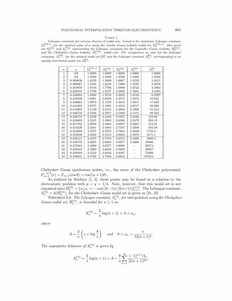
TABLE 1Lebesgue constants for various choices of nodal sets. Listed is the minimum Lebesgue constant,

ΛJGL,αn , for the optimal value of α using the Jacobi–Gauss–Lobatto nodal set, ΠJGL,α

n . Also givenare ΛLGL

n and ΛCGLn representing the Lebesgue constants for the Legendre–Gauss–Lobatto, ΠLGL

n ,and the Chebyshev–Gauss–Lobatto, ΠCGL

n , nodal sets. For comparison we also list the Lebesgueconstants, ΛOpt

n , for the optimal nodal set [27] and the Lebesgue constant, ΛEqn , corresponding to an

equally distributed nodal set, ΠEqn .

n α ΛJGL,αn ΛLGL

n ΛCGLn ΛOpt

n ΛEqn

1 All 1.0000 1.0000 1.0000 1.0000 1.00002 All 1.2500 1.2500 1.2500 1.2500 1.25003 0.364636 1.4229 1.5000 1.6667 1.4229 1.63114 0.390667 1.5595 1.6359 1.7988 1.5595 2.20785 0.410978 1.6746 1.7786 1.9889 1.6722 3.10636 0.420531 1.7709 1.8737 2.0826 1.7681 4.54937 0.428904 1.8560 1.9724 2.2022 1.8516 6.92978 0.433838 1.9301 2.0456 2.2747 1.9255 10.9459 0.438665 1.9973 2.1210 2.3619 1.9917 17.848

10 0.441695 2.0575 2.1805 2.4210 2.0517 29.89911 0.444993 2.1129 2.2415 2.4894 2.1066 51.21412 0.446733 2.1636 2.2917 2.5393 2.1571 89.32413 0.448718 2.2109 2.3428 2.5957 2.2040 158.0914 0.450689 2.2545 2.3862 2.6388 2.2476 283.1915 0.451792 2.2958 2.4303 2.6867 2.2884 512.3516 0.453426 2.3341 2.4684 2.7247 2.3268 934.5017 0.453893 2.3707 2.5072 2.7664 2.3630 1716.418 0.454938 2.4049 2.5412 2.8003 2.3973 3171.119 0.456111 2.4375 2.5758 2.8371 2.4298 5889.420 0.456752 2.4685 2.6065 2.8677 2.4608 10986.21 0.457683 2.4980 2.6377 2.9008 - 20574.22 0.459342 2.5260 2.6658 2.9288 - 38667.23 0.459593 2.5532 2.6942 2.9587 - 72908.24 0.459831 2.5792 2.7200 2.9844 - 137852.

Chebyshev–Gauss quadrature points, i.e., the zeros of the Chebyshev polynomial,P−1/2n+1 (x) = Tn+1(cos θ) = cos((n+ 1)θ).

As realized by Stieltjes [1, 2], these points may be found as a solution to theelectrostatic problem with p = q = 1/4. Note, however, that this nodal set is notcanonical since ΠCG

n = {xi|xi = − cos((2i−1)π/2(n+1))}n+1i=1 . The Lebesgue constant,

ΛCGn = Λ(ΠCG

n ), for the Chebyshev–Gauss nodal set is given as [21, 22]THEOREM 3.4. The Lebesgue constant, ΛCG

n , for interpolation using the Chebyshev–Gauss nodal set, ΠCG

n , is bounded for n ≥ 1 as

ΛCGn =

2π

log(n+ 1) +A+ αn,

where

A =2π

(γ + log

8π

)and 0 < αn <

π

72(n+ 1)2 .

The asymptotic behavior of ΛCGn is given by

ΛCGn ' 2

πlog(n+ 1) +A+

8π

∞∑s=1

(−1)s+1As[2(n+ 1)]2s

,

662 J. S. HESTHAVEN

where

As =(22s−1 − 1

)2 π2s

2sB2

2s

(2s)!,

and Bp signifies the Bernoulli numbers.Comparing with the optimal values of the Lebesgue constant given in Theorem

3.2, is it clear that interpolation using ΠCGn results in an approximation error being

close to that of the optimal canonical nodal set.However, if we consider the canonical Chebyshev–Gauss or extended Chebyshev–

Gauss nodal set, ΠECGn , obtained through the linear mapping

ΠECGn =

xi∣∣∣∣∣∣xi = −

cos(

2i−12(n+1)π

)cos(

π2(n+1)

)n+1

i=1

,

the Lebesgue constant, ΛECGn = Λ(ΠECG

n ), is bounded by [21].THEOREM 3.5. The Lebesgue constant, ΛECG

n , for interpolation using the extendedChebyshev–Gauss nodal set, ΠECG

n , is bounded for n ≥ 4 as

ΛECGn =

2π

log(n+ 1) +A− 43π

+ βn,

where

0 < βn < 0.01[log(n+ 1

4

)]−1

.

By expressing the two constants in Theorems 3.4 and 3.5 as

A− χ =2π

log 2 and A− 43π− χ =

2π

(log 2− 2

3

)= 0.01685801 . . . ,

it becomes clear that both nodal sets are close to the optimal set for large values ofn. However, in particular, the extended Chebyshev–Gauss nodal set, ΠECG

n , resultsin an approximation that is very close to that obtained using the optimal nodal set.Indeed, to the best of our knowledge, the extended Chebyshev–Gauss nodal set is thebest-known nodal set with the position of the nodes given on closed form.

However, ΠECGn does not represent a nodal set associated with the zeros of a

Jacobi polynomial. As discussed previously, this issue is important in connectionwith the solution of partial differential equations using spectral methods where high-order integration is required. Consequently, in such cases it is desirable that thenodal set be related to a Gauss quadrature formula, explaining why the extendedChebyshev–Gauss nodal set plays a less important role in this context.

Also, the Chebyshev–Gauss nodal set is less attractive for use in connection withspectral methods as the endpoints of the interval are not included, thereby makingit hard to enforce boundary conditions. For these reasons, the most used nodal setfor constructing approximate solutions to partial differential equations using spectralmethods is the canonical Chebyshev–Gauss–Lobatto set obtained as the zeros of thepolynomial, (1−x2)T ′n(x), and given in closed form as ΠCGL

n = (−1, {xi}ni=2, 1) wherexi = − cos((i− 1)π/n).


To return to the electrostatic analogy, we recall that the Jacobi–Gauss quadraturepoints appear from the original work. However, since the Jacobi–Gauss–Lobattoquadrature points are obtained as the interior zeros of the polynomial (Pαn (x))′ andusing the identity for Jacobi polynomials [23],

2d

dxPαn (x) = (n+ 1 + 2α)Pα+1

n−1 (x),

we realize also that the Jacobi–Gauss–Lobatto quadrature points appear as solutionsto the original electrostatic problem by using the relation α = 2(p− 1) and includingthe endpoints in the nodal set; e.g., using p = q = 3

4 results in the Chebyshev–Gauss–Lobatto nodal set (α = − 1

2 ).Estimation of the Lebesgue constant, ΛCGL

n = Λ(ΠCGLn ), for the Chebyshev–

Gauss–Lobatto nodal set is done in [24], yielding the following result.THEOREM 3.6. The Lebesgue constant, ΛCGL

n , using the Chebyshev–Gauss–Lobattonodal set, ΠCGL

n , is bounded as

ΛCGLn < ΛCG

n−1 n even,ΛCGLn = ΛCG

n−1 n odd,

where ΛCGn represents the Lebesgue constant obtained for the Chebyshev–Gauss nodal

set, ΠCGn , as given in Theorem 3.4.

We immediately observe that in addition to the desirable property that the Gauss–Lobatto nodal sets include the endpoints of S1, the Lebesgue constants are also uni-formly bounded by those obtained using the Gauss nodal set.

The tight bound on ΛCGLn for n being odd is possibly due to the observation [24]

that ΛCGLn = λ(ΠCGL

n , 0), where λ(ΠCGLn , x) represents the Lebesgue function. Based

on extensive numerical evidence, we conjecture as follows.CONJECTURE 3.1. The Lebesgue constant, ΛCGL

n , using the Chebyshev–Gauss–Lobatto nodal set, ΠCGL

n , is given as

n even : ΛCGLn = λ

(ΠCGLn ,

π

2n

), n→∞.

For n being even, x = 0 is always part of the nodal set as xn/2. Consequently, itis conjectured that the Lebesgue function attains its maximum value exactly betweenthe center node, xn/2, and x(n+2)/2, since

x(n+2)/2

2= −1

2cos(π

2n+ 2n

)=

12

sin(πn

)∼ π

2n

for large values of n. This result conforms well with the result that for n being odd,the maximum of the Lebesgue function is also found exactly between the two centernodes, i.e., at x = 0.

Values of the Lebesgue constant, ΛCGLn , are given in Table 1 for n ∈ [1, 24], and

in Fig. 1 we plot ΛCGLn for large n, confirming the logarithmic dependence on n.

Legendre distributed nodal sets. Based on the general expression for theinterpolating Lagrange polynomials, (2), it appears that the nodal set maximizingthe Vandermonde determinant, |VDM|, could be expected to yield an interpolatingpolynomial with a small value of the Lebesgue constant. As shown in [25], this nodalset is given as ΠLGL

n = (−1, {xi}ni=2, 1) where {xi}ni=2 = {xi|(P 0n(xi))′ = 0}ni=2, i.e.,

the extrema of P 0n(x) also known as the Legendre polynomial. This nodal set, ΠLGL

n ,is known as the Legendre–Gauss–Lobatto or the Fekete/Fejer nodal set.

664 J. S. HESTHAVEN

0 100 200 300 400 5001.0

1.5

2.0

2.5

3.0

3.5

4.0

4.5

5.0

Λn

n

ΛnLGL

ΛnCGL

ΛnUGL

FIG. 1. The Lebesgue constants as a function of n for various choices of Jacobi–Gauss–Lobattonodal sets. Shown are the Lebesgue constants for the Legendre polynomials, ΛLGL

n , and for Chebyshevpolynomials of the first, ΛCGL

n , and second kind, ΛUGLn , respectively.

Estimates for the Lebesgue constant, ΛLGLn = Λ(ΠLGL

n ), are sparse, the problembeing that no explicit formula for the nodal set is known. The first estimate is possiblygiven in [25] as ΛLGL

n ≤√n+ 1, which is also obtained simply by applying the

Cauchy–Schwartz inequality and the fact∑n+1i=1 |Li(ΠLGL

n , x)|2 ≤ 1. This, however,is very pessimistic, as evidenced by the conjecture in [13] that ΛLGL

n < ΛCGn and the

estimate ΛLGLn ≤ c log(n + 1) put forward in [26], although the constant, c, remains

undetermined. Based on numerical experiments, we conjecture the following.CONJECTURE 3.2. The Lebesgue constant, ΛLGL

n , using the Legendre–Gauss–Lobatto nodal set, ΠLGL

n , is bounded as

ΛLGLn ≤ 2

πlog(n+ 1) + 0.685,

and

ΛLGLn = λ(ΠLGL

n , 0) n odd,

ΛLGLn ' λ

(ΠLGLn , π2n

)n even.

This conjecture is consistent with those put forward in [13] and does indeedconfirm that ΛLGL

n < ΛCGn uniformly in n. Additionally, we also find ΛLGL

n < ΛCGLn

uniformly in n, as is illustrated in Fig. 1. Numerical values of ΛLGLn are given in

Table 1 for n ∈ [1, 24], supporting the conjecture.

Jacobi distributed nodal sets. Let us finally focus our attention on the generalcase, about which very little is known. If we first consider the Jacobi–Gauss nodalset, ΠJG,α

n , being given as ΠJG,αn = {xi|Pαn+1(xi) = 0}n+1

i=1 , the most general result is[3].


THEOREM 3.7. The Lebesgue constant, ΛJG,αn , using the Jacobi–Gauss nodal set,

ΠLGLn , scales as

ΛJG,αn ∼ O(log(n+ 1)) α ≤ − 1

2 ,

ΛJG,αn ∼ O(

√n+ 1) α > − 1

2 .

Unfortunately, no such general results exist when considering the nodal sets,ΠJGL,αn , based on the Jacobi–Gauss–Lobatto quadrature points, given as ΠJGL,α

n =(−1, {xi}ni=2, 1) where we have {xi}ni=2 = {xi|(Pαn (xi))′ = 0}ni=2. We have previouslydiscussed the two special cases of the Chebyshev–Gauss–Lobatto nodal set, α = −1/2,and the Legendre–Gauss–Lobatto nodal set, α = 0. An interesting question arises:among all ΠJGL,α

n , which value of α minimizes the Lebesgue constant, ΛJGL,αn , for a

given n?In attempting to address this question, we give in Table 1 the value of α leading

to the minimum Lebesgue constant, ΛJGL,αn , among all the nodal sets based on the

Jacobi–Gauss–Lobatto quadrature points, ΠJGL,αn , for various values of n. By com-

paring this with the Lebesgue constants, ΛOptn , for the optimal nodal set [27], is it

clear that the computed Jacobi–Gauss–Lobatto nodal sets are very close to the opti-mal nodal set? We observe that the value of α leading to the optimal nodal set varieswith n, although it seems that it asymptotes towards a fixed value around α ' 0.5.This tendency is found to be maintained for n ≤ 60. However, we have been unableto continue the computation beyond this point, as the computation of the optimalvalue of α becomes prohibitively expensive due to the many required computationsof the corresponding Lebesgue constant.

The value of α = 1/2 corresponds to a nodal set, ΠUGLn , based on the Gauss–

Lobatto quadrature points for the Chebyshev polynomial of the second kind beinggiven as Un(cos(θ)) = sin((n + 1)θ)/ sin θ. Unfortunately, as we will see shortly, thehypothesis that ΠUGL

n is close to the optimal nodal set is only valid for small n. Werecall that the nodal set is given in explicit form as ΠUGL

n = {−1, {xi}ni=2, 1} wherexi = − cos((2i− 1)π/2(n+ 1)).

We are not aware of any results estimating the Lebesgue constant, ΛUGLN =

Λ(ΠUGLn ), using the Gauss–Lobatto nodal set of the Chebyshev polynomials of the

second kind. Based on extensive numerical studies, we conjecture the following.CONJECTURE 3.3. The Lebesgue constant, ΛUGL

n , using the Chebyshev–Gauss–Lobatto nodal set, ΠUGL

n , is bounded as

ΛUGLn ≤ 2

πlog(n+ 1) + βn,

with

0 < βn < 0.525f(n+ 1),

where f is a weak function of n behaving asymptotically as

n→∞ :f(n)logn

→∞ ,f(n)√n→ 0.

We have been unable to estimate the unknown function, f(n), more accurately.However, numerical studies indicate that, asymptotically, f(n) ' nα, where α ∼O(0.1).

666 J. S. HESTHAVEN

(-1,0) (1,0)

(0,√3)_

S2l1 l2

l3

FIG. 2. The standard equilateral triangle, S2.

We observe that for small values of n, the nodal sets associated with Chebyshevpolynomials of the second kind results in a Lebesgue constant that is very close tothe optimal one as given in Theorem 3.2. However, the slow growth of ΛUGL

n withn renders this property invalid for increasing n. In Fig. 1 we compare ΛUGL

n withΛLGLn and ΛCGL

n to find that the former is superior to the more commonly usedChebyshev–Gauss–Lobatto points for any practical value of n, while it is superior tothe Legendre–Gauss–Lobatto points only for small n. An attractive property of ΠUGL

n

is, however, that it is given in explicit form contrary to ΠLGLn .

In the present section we have summarized and extended the results for inter-polation on nodal sets with particular emphasis on nodal sets appearing as solutionsto an electrostatic problem and related to the symmetric Jacobi polynomials. Theresults may most easily be summarized as

ΛEqn > ΛCG

n > ΛCGLn > ΛLGL

n ∼ ΛUGLn > ΛECG

n ,

which we believe is valid for all practical values of n in the context of spectral methodsand is consistent with results put forward in [13, 28].

Although there remain many open questions when considering interpolation inS1 using Jacobi–Gauss–Lobatto nodal sets, it seems clear, however, that some of thenodal sets obtainable through the solution of an electrostatic problem are very closeto what is theoretically possible.

4. Interpolation points in S2 using electrostatics. The problem of poly-nomial interpolation in S2 is considerably more complex than in S1 and very littleis known. Hence, in the present work we shall focus our attention on polynomialinterpolation of functions defined on an equilateral triangle, S2, as pictured in Fig. 2.

In the present context, it is convenient to use barycentric coordinates. Let usdenote vi, i ∈ [1, 3], as the three vertices; i.e., in this case v1 = (−1, 0), v2 = (0,

√3),

and v3 = (1, 0), such that any x ∈ S2 can be expressed using a convex combinationof the barycentric coordinates, (b1, b2, b3), as

x =3∑i=1

vibi and3∑i=1

bi = 1,

and 0 ≤ bi ≤ 1.


We introduce the polynomial space, P2n = span{pij(x) = xiyj ; i, j ≥ 0; i+ j ≤ n}.

The basis functions spanning the polynomial space may conveniently be thought ofas

1x y

x2 xy y2

x3 x2y y2x y3

...

Estimation of the Lebesgue constant for interpolation in S2 is extremely difficult,and, only for the equidistant grid in barycentric coordinates given as

ΠEqn =

{xi

∣∣∣∣(b1, b2, b3) =(

1− k + l

n,k

n,l

n

); k ≥ 0, l ≥ 0, k + l ≤ n

}Ni=1

,

do results exist. We recall that n represents the order of the polynomial approximationand also signifies the order of the polynomial employed along the edges. The explicitexpression for the interpolating Lagrange polynomial, Li(ΠEq

n ,x), is given in [29],where the bound for the Lebesgue constant, ΛEq

n , is derived also.THEOREM 4.1. The Lebesgue constant, ΛEq

n , using the nodal set, ΠEqn , for poly-

nomial interpolation in S2 is bounded as

ΛEqn ≤

(2n− 1n

).

As for interpolation along the line, we observe extremely rapid growth of ΛEqn ,

essentially rendering this nodal set useless for high-order polynomial interpolation.For reasons of comparison, we list the Lebesgue constants for n ∈ [1, 16] in Table 2.The question naturally raises as to whether it is possible to obtain nodal sets bettersuited than ΠEq

n for interpolation in S2.This question was first addressed in [29] by realizing from (2) that a good nodal set

could be obtained by maximizing the Vandermonde determinant, |VDM|, much likethe procedure that leads to the Legendre–Gauss–Lobatto points discussed previously.However, the study was quite restricted and nodal sets were computed only for n ≤ 7.

Recently, a more thorough study was published in [27], where nodal sets, resultingin a significantly slower growth of the Lebesgue constant than obtained for ΠEq

n , wereobtained by minimizing over the L2-norm of the Lebesgue function for n ∈ [2, 13]. Asis evident from the computed Lebesgue constants, ΛOpt

n , as reproduced in Table 2,the suggested procedure yields very good nodal sets, although there is no way one canknow whether these are the optimal sets. Indeed, as we will show shortly, at least forn ≤ 5 is it possible to find sets with a smaller Lebesgue constant. However, the mainreason for our interest in obtaining alternative nodal sets is the fact that those given in[27] do not have nodal distributions along the edges that can be identified as Jacobi–Gauss–Lobatto quadrature points. As we have argued previously, this latter propertyis advantageous if one wishes to apply the polynomials on the simplex in connectionwith spectral methods which are almost exclusively based on Jacobi polynomials.

Inspired by the success of polynomial interpolation in S1, when using nodal setsappearing as solutions to an electrostatic problem, we now propose to consider thefollowing scenario.

Assume that the edges of the simplex, S2, labeled ll as illustrated in Fig. 2, arefragments of a continuous line charge with the charge density, ρLl > 0. Consider now

668 J. S. HESTHAVEN

an arbitrary edge, ll, connecting the two vertices, va = (xa, ya) and vb = (xb, yb).The electrostatic force, F l(x), from the line acting on a particle with the charge, ρp,held at the position x, is then given as FLl (x) = ρpE

Ll (x) = −ρp∇φLl , where φLl is

the electrostatic potential from the edge, ll. Contrary to the approach used for S1,where the potential is logarithmic, we assume the potential to be algebraic, such thatthe potential from the line fragment at x is given as

φLl (x) = ρLl

∫ 1

0

1|x− xL|

dt,

where xL = va + t(vb − va), t ∈ [0, 1], represents the edge. It is straightforward toperform this integration analytically.

We also assume that a number, Np, of unit mass charges, ρp, are allowed to movefreely inside the simplex, mutually interacting according to the potential

φ(xi,xj) =ρ2p

|xi − xj |.

Let us now propose to consider the following problem.

Problem: Let the line charge density be given as ρLl > 0. Assume also that Npunit mass charges with unit charge, ρp = 1, are allowed to move freely insidethe simplex. What is the steady state position of the charges that minimizesthe electrostatic energy

W (x1, . . . ,xNp) =Np∑i=1

3∑l=1

φLl (xi) +12

Np∑j=1j 6=i

φ(xi,xj)

.

The problem is clearly very similar to the one originally put forward by Stieltjes [1, 2],however, with significantly more complexity.

Contrary to the m = 1 case, we have no prior knowledge of a proper choice ofthe line charge density of the line, ρLl , in order to obtain nodal sets well suited forpolynomial interpolation. Indeed, we will later use this free parameter for optimizingthe nodal sets. However, based on the knowledge gained from S1, we believe thatthe most appropriate choice is ρL1 = ρL2 = ρL3 = ρL; i.e., the external potential fieldimposed by the line charges is symmetric.

As the aim is to construct nodal sets well suited for approximating partial differen-tial equations in a multidomain setting, we require that the edges contain interpolationpoints. However, the specification of these points is at this point undetermined.

We also recall that the aim is to construct interpolating polynomials with the edgepolynomials having the same order as that of the global interpolating polynomials;i.e., the total number of nodal points should be related to the number of freely movingcharges as Np = N2

n − 3n, where 3n is the number of nodal points reserved for theedges. This value of Np allows for the construction of a complete basis as discussedin section 2.

We have chosen to approach the problem by solving it numerically as an N -bodyproblem by integrating Newtons second law as

xi = −

3∑l=1

∇φLl (xi) +Np∑j=1j 6=i

∇φ(xi,xj)

− εxi,


where the last term, xi, corresponds to a small friction in order to make the prob-lem slightly dissipative. This equation is advanced in time using a 7(6) embeddedNystrom–Runge–Kutta scheme with error control [30]. The resulting solution ispassed on as an initial guess to a nonlinear solver to find the true steady state solution.We have used an algorithm based on a modification of Powell’s hybrid algorithm [31].

The single most important remaining point is how to choose the initial conditions.Finding the global minimum of the energy function is in general extremely compli-cated, in particular for increasing Np. However, since we are interested in solutionssuitable for polynomial interpolation, we restrict our attention to steady state solu-tions that possess a high degree of symmetry. Inside the simplex, we consider solutionsthat are constructed of three symmetry patterns [27]. A charge can be situated atthe center of the triangle, termed a 1-symmetry; it can be positioned along one of thethree meridians, termed a 3-symmetry; or it can be inside one of the six subtrianglesbounded by the symmetry axes, referred to as a 6-symmetry. If we denote the num-ber of charges with a 1-symmetry, n1, the number of charges with a 3-symmetry, n3,and those with a 6-symmetry as n6, the total number of charges is then obtained asNp = (n− 1)(n− 2)/2 = n1 + 3n3 + 6n6.

The integer solution to this equation is nonunique for n > 4. Different solutionscorrespond to different symmetry patterns inherent in the distribution of the charges.We have used these initial symmetry patterns to construct the initial conditions andthen searched for the specific symmetry pattern that results in a steady state solutionwith the minimum energy among all the possible symmetry patterns for a given n.

Having established the computational framework, let us now return to the twooutstanding problems: specification of the line charge, ρL, and the distribution of thenodes along the edges. As mentioned previously, we are primarily interested in havinga distribution of nodal points along the edges that is related to Jacobi–Gauss–Lobattoquadrature points; i.e., they are uniquely determined by the parameter, α, of theJacobi polynomial. At this point we realize that the problem of finding the best nodaldistribution inside the simplex is reduced to a two-parameter minimization problemin ρL and α. This is much like the original problem, however, with the unfortunatedifference that in S2 we do not know how they are related or even if they are.

In the following we have used the approach outlined above to find symmet-ric, steady state solutions to the electrostatic problem. However, doing a full two-dimensional optimization is out of reach and we have restricted our attention to a fewspecial cases of α that are most interesting within the present context.

For a fixed value of α, the problem is reduced to a one-dimensional minimizationproblem in ρL, which is feasible. In all problems we find that ρL ∼ O(1) but variesslightly with n as well as with α.

As the most natural choice of α in relation to spectral methods, we have computedthe nodal sets for α = −1/2, corresponding to the Chebyshev–Gauss–Lobatto nodalset along the edge. In Table 2, we give the corresponding Lebesgue constant, ΛCGL

n ,for increasing n, confirming the soundness of the electrostatic approach. Indeed, weobserve that the computed nodal sets are very good as compared to the correspondingequidistant nodal set, and they also compare well with the nodal sets presented in [27],indeed being superior for small values of n. In Appendix A we give the barycentriccoordinates for the computed nodal sets for n ∈ [2, 16].

Another widely used nodal set for spectral methods is based on the Legendre–Gauss–Lobatto nodal set, i.e., corresponding to α = 0. We have obtained nodal setswith the Legendre–Gauss–Lobatto nodal set along the edges and the corresponding

670 J. S. HESTHAVEN

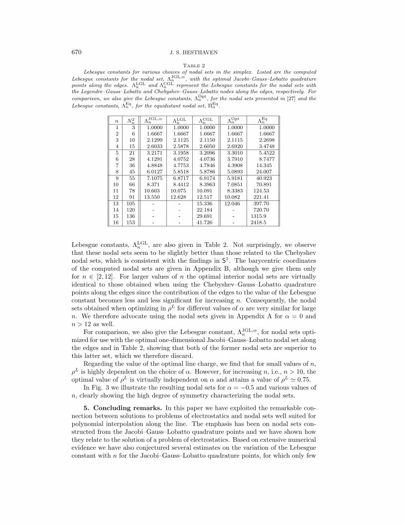
TABLE 2Lebesgue constants for various choices of nodal sets in the simplex. Listed are the computed

Lebesgue constants for the nodal set, ΛJGL,αn , with the optimal Jacobi–Gauss–Lobatto quadrature

points along the edges. ΛLGLn and ΛCGL

n represent the Lebesgue constants for the nodal sets withthe Legendre–Gauss–Lobatto and Chebyshev–Gauss–Lobatto nodes along the edges, respectively. Forcomparison, we also give the Lebesgue constants, ΛOpt

n , for the nodal sets presented in [27] and theLebesgue constants, ΛEq

n , for the equidistant nodal set, ΠEqn .

n N2n ΛJGL,α

n ΛLGLn ΛCGL

n ΛOptn ΛEq

n

1 3 1.0000 1.0000 1.0000 1.0000 1.00002 6 1.6667 1.6667 1.6667 1.6667 1.66673 10 2.1299 2.1125 2.1150 2.1115 2.26984 15 2.6033 2.5878 2.6050 2.6920 3.47485 21 3.2171 3.1958 3.2096 3.3010 5.45226 28 4.1291 4.0752 4.0736 3.7910 8.74777 36 4.8848 4.7753 4.7846 4.3908 14.3458 45 6.0127 5.8518 5.8786 5.0893 24.0079 55 7.1075 6.8717 6.9174 5.9181 40.923

10 66 8.371 8.4412 8.3963 7.0851 70.89111 78 10.603 10.075 10.091 8.3383 124.5312 91 13.550 12.628 12.517 10.082 221.4113 105 - - 15.336 12.046 397.7014 120 - - 22.184 - 720.7015 136 - - 29.691 - 1315.916 153 - - 41.726 - 2418.5

Lebesgue constants, ΛLGLn , are also given in Table 2. Not surprisingly, we observe

that these nodal sets seem to be slightly better than those related to the Chebyshevnodal sets, which is consistent with the findings in S1. The barycentric coordinatesof the computed nodal sets are given in Appendix B, although we give them onlyfor n ∈ [2, 12]. For larger values of n the optimal interior nodal sets are virtuallyidentical to those obtained when using the Chebyshev–Gauss–Lobatto quadraturepoints along the edges since the contribution of the edges to the value of the Lebesgueconstant becomes less and less significant for increasing n. Consequently, the nodalsets obtained when optimizing in ρL for different values of α are very similar for largen. We therefore advocate using the nodal sets given in Appendix A for α = 0 andn > 12 as well.

For comparison, we also give the Lebesgue constant, ΛJGL,αn , for nodal sets opti-

mized for use with the optimal one-dimensional Jacobi–Gauss–Lobatto nodal set alongthe edges and in Table 2, showing that both of the former nodal sets are superior tothis latter set, which we therefore discard.

Regarding the value of the optimal line charge, we find that for small values of n,ρL is highly dependent on the choice of α. However, for increasing n, i.e., n > 10, theoptimal value of ρL is virtually independent on α and attains a value of ρL ' 0.75.

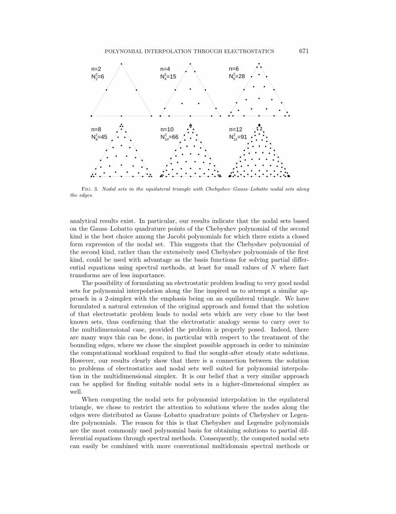
In Fig. 3 we illustrate the resulting nodal sets for α = −0.5 and various values ofn, clearly showing the high degree of symmetry characterizing the nodal sets.

5. Concluding remarks. In this paper we have exploited the remarkable con-nection between solutions to problems of electrostatics and nodal sets well suited forpolynomial interpolation along the line. The emphasis has been on nodal sets con-structed from the Jacobi–Gauss–Lobatto quadrature points and we have shown howthey relate to the solution of a problem of electrostatics. Based on extensive numericalevidence we have also conjectured several estimates on the variation of the Lebesgueconstant with n for the Jacobi–Gauss–Lobatto quadrature points, for which only few


n=2N2

2=6n=4N4

2=15n=6N6

2=28

n=8N8

2=45n=10N2

10=66n=12N2

12=91

FIG. 3. Nodal sets in the equilateral triangle with Chebyshev–Gauss–Lobatto nodal sets alongthe edges.

analytical results exist. In particular, our results indicate that the nodal sets basedon the Gauss–Lobatto quadrature points of the Chebyshev polynomial of the secondkind is the best choice among the Jacobi polynomials for which there exists a closedform expression of the nodal set. This suggests that the Chebyshev polynomial ofthe second kind, rather than the extensively used Chebyshev polynomials of the firstkind, could be used with advantage as the basis functions for solving partial differ-ential equations using spectral methods, at least for small values of N where fasttransforms are of less importance.

The possibility of formulating an electrostatic problem leading to very good nodalsets for polynomial interpolation along the line inspired us to attempt a similar ap-proach in a 2-simplex with the emphasis being on an equilateral triangle. We haveformulated a natural extension of the original approach and found that the solutionof that electrostatic problem leads to nodal sets which are very close to the bestknown sets, thus confirming that the electrostatic analogy seems to carry over tothe multidimensional case, provided the problem is properly posed. Indeed, thereare many ways this can be done, in particular with respect to the treatment of thebounding edges, where we chose the simplest possible approach in order to minimizethe computational workload required to find the sought-after steady state solutions.However, our results clearly show that there is a connection between the solutionto problems of electrostatics and nodal sets well suited for polynomial interpola-tion in the multidimensional simplex. It is our belief that a very similar approachcan be applied for finding suitable nodal sets in a higher-dimensional simplex aswell.

When computing the nodal sets for polynomial interpolation in the equilateraltriangle, we chose to restrict the attention to solutions where the nodes along theedges were distributed as Gauss–Lobatto quadrature points of Chebyshev or Legen-dre polynomials. The reason for this is that Chebyshev and Legendre polynomialsare the most commonly used polynomial basis for obtaining solutions to partial dif-ferential equations through spectral methods. Consequently, the computed nodal setscan easily be combined with more conventional multidomain spectral methods or

672 J. S. HESTHAVEN

TABLE 3

n n1 n2 n3 b1 b2 b33 1 0.3333333333 0.3333333333 0.33333333334 1 0.2410021998 0.2410021998 0.51799560045 2 0.1591570023 0.1591570023 0.6816859954

0.4099016620 0.4099016620 0.18019667606 1 0.3333333333 0.3333333333 0.3333333333

1 0.1048904342 0.1048904342 0.79021913161 0.3095036860 0.5582114022 0.1322849118

7 3 0.0666479037 0.0666479037 0.86670419240.4474963910 0.4474963910 0.10500721800.2606379453 0.2606379453 0.4787241094

1 0.2328951264 0.6750593997 0.09204547398 3 0.0467325482 0.0467325482 0.9065349036

0.2031909379 0.2031909379 0.59361812420.3906323571 0.3906323571 0.2187352858

2 0.3618069634 0.5544121321 0.08378090450.1799524415 0.7523326932 0.0677148653

9 1 0.3333333333 0.3333333333 0.33333333333 0.0354284515 0.0354284515 0.9291430970

0.4641239296 0.4641239296 0.07175214080.1632684184 0.1632684184 0.6734631632

3 0.2965866112 0.6351919517 0.06822143710.1437685751 0.8034472485 0.05278417640.3225938344 0.4969468296 0.1804593360

10 4 0.0267617465 0.0267617465 0.94647650700.1333154550 0.1333154550 0.73336909000.4230209738 0.4230209738 0.15395805240.2834641787 0.2834641787 0.4330716426

4 0.3934497870 0.5469389728 0.05961124020.2464304982 0.6986850110 0.05488449080.1165696792 0.8422416956 0.04118862520.2707661899 0.5807728926 0.1484609175

11 5 0.0205770993 0.0205770993 0.95884580140.4745463805 0.4745463805 0.05090723900.1106491928 0.1106491928 0.77870161440.2422912395 0.2422912395 0.51541752100.3764104927 0.3764104927 0.2471790146

5 0.3362467835 0.6143637919 0.04938942460.2075057639 0.7480004251 0.04449381100.0961598440 0.8711975595 0.03264259650.3648517435 0.5058451075 0.12930314900.2299937315 0.6463450688 0.1236611997

12 1 0.3333333333 0.3333333333 0.33333333334 0.0157664060 0.0157664060 0.9684671880

0.0927641836 0.0927641836 0.81447163280.4451055330 0.4451055330 0.10978893400.2092594550 0.2092594550 0.5814810900

7 0.4144591572 0.5428398510 0.04270099180.2891782274 0.6704310002 0.04039077240.1766396330 0.7874226099 0.03593775710.0801575546 0.8939792746 0.02586317080.3176588844 0.5750391576 0.10730195800.1970549373 0.6986253330 0.10431972970.3292289528 0.4566354051 0.2141356421

even provide the basic building block for a triangular spectral element method withunstructured grids interior to the triangle [32].

Appendix A: Nodal matrix for the triangle with Chebyshev–Gauss–Lobatto nodal sets along the edges. In Tables 3–5 we give the barycentric co-


TABLE 4

n n1 n2 n3 b1 b2 b313 6 0.0125158559 0.0125158559 0.9749682882

0.4814041934 0.4814041934 0.03719161320.0791069148 0.0791069148 0.84178617040.1831015613 0.1831015613 0.63379687740.4068245409 0.4068245409 0.18635091820.2954002632 0.2954002632 0.4091994736

8 0.3615540438 0.6022119116 0.03623404460.2513189999 0.7149811088 0.03369989130.1523482839 0.8179762698 0.02967544630.0680753374 0.9108476566 0.02107700600.3944786597 0.5151527485 0.09036859180.2767319260 0.6304802457 0.09278782830.1706952037 0.7399484931 0.08935630320.2915934740 0.5215057084 0.1869008176

14 6 0.4587977340 0.4587977340 0.08240453200.3671908093 0.3671908093 0.26561838140.2595748224 0.2595748224 0.48085035520.1603773315 0.1603773315 0.67924533700.0685768901 0.0685768901 0.86284621980.0103478215 0.0103478215 0.9793043570

10 0.9234057833 0.0588664441 0.01772777260.8416660290 0.1330619104 0.02527206070.7521462903 0.2191316332 0.02872207640.6425344401 0.3256595455 0.03180601440.5379997781 0.4292596705 0.03274055130.4692799339 0.3610693351 0.16965073100.7721478696 0.1494014554 0.07845067500.5652822600 0.3505856755 0.08413206450.6781794781 0.2494595411 0.07236098080.5834887797 0.2550816171 0.1614296032

15 1 0.3333333333 0.3333333333 0.33333333336 0.4852528832 0.4852528832 0.0294942336

0.4255990820 0.4255990820 0.14880183600.2320836842 0.2320836842 0.53583263160.1405179457 0.1405179457 0.71896410860.0599963506 0.0599963506 0.88000729880.0085857218 0.0085857218 0.9828285564

12 0.9337196169 0.0512926813 0.01498770180.8617284617 0.1169291070 0.02134243130.7794706504 0.1957424109 0.02478693870.6834546988 0.2890601702 0.02748513100.5886608293 0.3824865582 0.02885261240.8006726315 0.1325472687 0.06678009980.7134213061 0.2207559648 0.06582272910.6135939037 0.3123505510 0.07405554530.5171616793 0.4145995177 0.06823880300.6286428956 0.2270147509 0.14434235350.5244220875 0.3265860871 0.14899182540.4324830342 0.3299898010 0.2375271649

ordinates for the nodal sets optimized for use with Chebyshev–Gauss–Lobatto nodalsets of order n along the edges; i.e., they are distributed as the zeros of the polynomial,(1−x2)T ′n(x). Only the nodes interior to the simplex are given, and nodes processingsymmetries are only given once. The remaining nodes can be found by permutationsof the barycentric coordinates.

674 J. S. HESTHAVEN

TABLE 5

n n1 n2 n3 b1 b2 b316 7 0.4692881367 0.4692881367 0.0614237267

0.3932305456 0.3932305456 0.21353890890.3025577746 0.3025577746 0.39488445090.2078492229 0.2078492229 0.58430155420.1284932701 0.1284932701 0.74301345980.0529388222 0.0529388222 0.89412235560.0072437614 0.0072437614 0.9855124772

14 0.9419105656 0.0452492885 0.01284014580.8772044870 0.1042200005 0.01857551250.8060459745 0.1727546471 0.02119937840.7198500717 0.2560058606 0.02414406770.6256312013 0.3487602527 0.02560854590.5343544917 0.4393591499 0.02628635840.8214366546 0.1173927115 0.06117063380.7464832409 0.1959218281 0.05759493090.6578452111 0.2860606787 0.05609411020.5620632423 0.3743524772 0.06358428050.6657283975 0.1263493158 0.20792228670.5755509622 0.2921362629 0.13231277490.4806452274 0.3853613574 0.13399341520.4883520007 0.2978352313 0.2138127680

TABLE 6

n n1 n2 n3 b1 b2 b33 1 0.3333333333 0.3333333333 0.33333333334 1 0.2371200168 0.2371200168 0.52575996645 2 0.1575181512 0.1575181512 0.6849636976

0.4105151510 0.4105151510 0.17896969806 1 0.3333333333 0.3333333333 0.3333333333

1 0.1061169285 0.1061169285 0.78776614301 0.3097982151 0.5569099204 0.1332918645

7 3 0.0660520784 0.0660520784 0.86789584320.4477725053 0.4477725053 0.10445498940.2604038024 0.2604038024 0.4791923952

1 0.2325524777 0.6759625951 0.09148492728 3 0.0469685351 0.0469685351 0.9060629298

0.2033467796 0.2033467796 0.59330644080.3905496216 0.3905496216 0.2189007568

2 0.3617970895 0.5541643672 0.08403854330.1801396087 0.7519065566 0.0679538347

9 1 0.3333333333 0.3333333333 0.33333333333 0.0355775717 0.0355775717 0.9288448566

0.4640303025 0.4640303025 0.07193939500.1633923069 0.1633923069 0.6732153862

3 0.2966333890 0.6349633653 0.06840324570.1439089974 0.8031490682 0.05294193440.3225890045 0.4968009397 0.1806100558

Appendix B: Nodal matrix for the triangle with Legendre–Gauss–Lobatto nodal sets along the edges. In Tables 6 and 7, we give the barycentriccoordinates for the nodal sets optimized for use with Legendre–Gauss–Lobatto nodalsets of order n along the edges; i.e., they are distributed as the zeros of the polynomial,(1−x2)P ′n(x). Only the nodes interior to the simplex are given and nodes processingsymmetries are only given once. The remaining nodes can be found by permutationsof the barycentric coordinates.


TABLE 7

n n1 n2 n3 b1 b2 b310 4 0.0265250690 0.0265250690 0.9469498620

0.1330857076 0.1330857076 0.73382858480.4232062312 0.4232062312 0.15358753760.2833924371 0.2833924371 0.4332151258

4 0.3934913008 0.5472380443 0.05927065490.2462883939 0.6991456238 0.05456598230.1163195333 0.8427538829 0.04092658380.2707097521 0.5811217960 0.1481684519

11 5 0.0204278105 0.0204278105 0.95914437900.4746683133 0.4746683133 0.05066337340.1104863580 0.1104863580 0.77902728400.2422268680 0.2422268680 0.51554626400.3764778430 0.3764778430 0.2470443140

5 0.3361965758 0.6146545276 0.04914889660.2073828199 0.7483396985 0.04427748160.0959885136 0.8715407373 0.03247074910.3649298091 0.5060795425 0.12899064840.2299163838 0.6466193522 0.1234642640

12 1 0.3333333333 0.3333333333 0.33333333334 0.0156346170 0.0156346170 0.9687307660

0.0926054449 0.0926054449 0.81478911020.4452623516 0.4452623516 0.10947529680.2091994115 0.2091994115 0.5816011770

7 0.4145270405 0.5430117044 0.04246125510.2890538328 0.6707932601 0.04015290710.1765067641 0.7877603302 0.03573290570.0799959921 0.8942989924 0.02570501550.3177076680 0.5753716491 0.10692068290.1969473706 0.6989024696 0.10415015980.3292603428 0.4567841256 0.2139555316

Acknowledgment. The author acknowledges many fruitful conversations withProf. D. Gottlieb and Dr. C. B. Quillen, Brown University. Comments from Dr. M.Carpenter, NASA Langley Research Center, are likewise highly appreciated.

REFERENCES

[1] T. J. STIELTJES, Sur quelques theoremes d’algebre, Comptes Rendus de l’Academie des Sci-ences, 100 (1885), pp. 439–440.

[2] T. J. STIELTJES, Sur les Polynomes de Jacobi, Comptes Rendus Acad. Sci., 100 (1885), pp.620–622.

[3] G. SZEGO, Orthogonal Polynomials, American Mathematical Society, 5th ed., Providence, RI,1975.

[4] C. CANUTO, M. Y. HUSSAINI, A. QUARTERONI, AND T. A. ZANG, Spectral Methods in FluidMechanics. Springer Series in Computational Physics, Springer-Verlag, Berlin, 1988.

[5] I. BABUSKA AND M. SURI, The p- and h-p version of the finite element method. An overview,Comput. Methods Appl. Mech. Engrg., 80 (1990), pp. 5–26.

[6] A. PATERA, A spectral element method for fluid dynamics: Laminar flow in a channel, J.Comput. Phys., 54 (1984), pp. 468–488.

[7] R. P. FEINERMAN AND D. J. NEWMAN, Polynomial Approximation, Williams and Wilkins,Baltimore, MD, 1974.

[8] K. CHUNG AND T. YAO, On lattices admitting unique Lagrange interpolations, SIAM J. Numer.Anal., 14 (1977), pp. 735–743.

[9] N. J. HIGHAM, Accuracy and Stability of Numerical Algorithms, SIAM, Philadelphia, PA, 1996.[10] P. J. DAVIS, Interpolation and Approximation, Dover Publications, New York, 1975.[11] T. J. RIVLIN, An Introduction to the Approximation of Functions, Dover, New York, 1969.[12] J. SZABADOS AND P. VERTESI, Interpolation of Functions, World Scientific, River Edge, NJ,

1990.

676 J. S. HESTHAVEN

[13] F. W. LUTTMANN AND T. J. RIVLIN, Some numerical experiments in the theory of polynomialinterpolation, IBM J. Res. Develop., 9 (1965), pp. 187–191.

[14] T. A. KILGORE, A characterization of the Lagrange interpolation projection with minimalTchebycheff norm, J. Approx. Theory, 24 (1978), pp. 273–288.

[15] C. DE BOOR AND A. PINKUS, Proof of the conjecture of Bernstein and Erdos concerning theoptimal nodes for polynomial interpolation, J. Approx. Theory, 24 (1978), pp. 289–303.

[16] J. R. ANGELOS, E. H. KAUFMAN JR., M. S. HENRY, AND T. D. LENKER, Optimal Nodes forPolynomial Interpolation, in Approximation Theory VI: Vol I, C. K. Chui, L. L. Schumaker,and J. D. Ward, eds., Academic Press, New York, 1989, pp. 17–20.

[17] P. ERDOS, Problem and Results on the Theory of Interpolation. II, Acta Math. Acad. Sci.Hungar., 12 (1961), pp. 235–244.

[18] A. H. TURETSKII, The bounding of polynomials prescribed at equally distributed points, Proc.Pedag. Inst. Vitebsk., 3 (1940), pp. 117–127.

[19] A. SCHONHAGE, Fehlerfortpflanzung bei Interpolation, Numer. Math., 3 (1961), pp. 62–71.[20] L. N. TREFETHEN AND J. C. WEIDEMAN, Two results on polynomial interpolation in equally

spaced points, J. Approx. Theory, 65 (1991), pp. 247–260.[21] R. GUNTTNER, Evaluation of Lebesgue constants, SIAM J. Numer. Anal., 17 (1980), pp.

512–520.[22] P. N. SHIVAKUMAR AND R. WONG, Asymptotic expansion of the Lebesgue constants associated

with polynomial interpolation, Math. Comp., 39 (1982), pp. 195–200.[23] A. ERDELYI, Higher transcendental functions, Vol. II, Robert Krieger, Melbourne, FL, 1953.[24] J. H. MCCABE AND G. M. PHILLIPS, On a Certain Class of Lebesgue Constants, BIT, 13

(1973), pp. 434–442.[25] L. FEJER, Lagrangesche Interpolation und die Zugehorigen Konjugierten Punkte, Math. Ann.,

106 (1932), pp. 1–55.[26] B. SUNDERMANN, Lebesgue Constants in Lagrangian Interpolation at the Fekete Points, Ergeb-

nisbericht der Lehrstuhle Math III, VIII, 40, Univ. Dortmunn, Germany, 1980.[27] Q. CHEN AND I. BABUSKA, Approximate optimal points for polynomial interpolation of real

functions in an interval and in a triangle, Comput. Methods Appl. Mech. Engrg., 128(1995), pp. 405–417.

[28] L. BRUTMAN, On the Lebesgue function for polynomial interpolation, SIAM J. Numer. Anal.,15 (1978), pp. 694–704.

[29] L. P. BOS, Bounding the Lebesgue function for interpolation in a simplex, J. Approx. Theory,38 (1983), pp. 43–59.

[30] E. HAIRER, S. P. NØRSETT, AND G. WANNER, Solving Ordinary Differential Equations I.Springer Series in Computational Mathematics 8, Springer-Verlag, Berlin, 1980.

[31] J. J. MORE, B. S. GARBOW, AND K. E. HILLSTROM, User Guide for MINPACK-1, ReportANL-80-74, Argonne National Laboratory, Argonne, IL, 1980.

[32] J. S. HESTHAVEN AND D. GOTTLIEB, Stable spectral methods for conservations laws on trian-gles with unstructured grids, SIAM J. Numer. Anal., 1997, submitted.

from electrostatics to almost optimal …vageli/courses/ma505/jan1.pdffrom electrostatics to almost...

Documents