from eeg signals to brain connectivity: a model-based
TRANSCRIPT

From EEG signals to brain connectivity: a model-based evaluation of interdependence measures
Fabrice Wendling 1,2 , Karim Ansari-Asl 3, Fabrice Bartolomei 4,5,6, Lotfi Senhadji 1,2
1 INSERM, U642, Rennes, F-35000, France
2 Université de Rennes 1, LTSI, F-35000, France
3 Shahid Chamran University, Faculty of Engineering, Ahvaz, Iran
4 INSERM, U751, Marseille, F-13000, France
5 AP-HM, Hôpital de la Timone, Service de Neurophysiologie Clinique, Marseille, F-13000, France
6 Aix Marseille Université, Faculté de Médecine, Marseille, F-13000, France
Corresponding author: [email protected]
Submitted to the Journal of Neuroscience MethodsSpecial issue on ‘(Multi-)frequency locking’
March 2009
REVISED VERSION – April 27, 2009
* Title page-incl. type of article and authors' name and affilia

2
Abstract
In the past, considerable effort has been devoted to the development of signal processing techniques aimed at
characterizing brain connectivity from signals recorded from spatially-distributed regions during normal or pa-
thological conditions. In this paper, three families of methods (linear and nonlinear regression, phase synchroni-
zation, and generalized synchronization) are reviewed. Their performances were evaluated according to a model-
based methodology in which a priori knowledge about the underlying relationship between systems that gener-
ate output signals is available. This approach allowed us to relate the interdependence measures computed by
connectivity methods to the actual values of the coupling parameter explicitly represented in various models of
signal generation. Results showed that: (i) some of the methods were insensitive to the coupling parameter; (ii)
results were dependent on signal properties (broad band versus narrow band); (iii) there was no “ideal” method,
i.e. none of the methods performed better than the other ones in all studied situations. Nevertheless, regression
methods showed sensitivity to the coupling parameter in all tested models with average or good performances.
Therefore, it is advised to first apply these “robust” methods in order to characterize brain connectivity before
using more sophisticated methods that require specific assumptions about the underlying model of relationship.
In all cases, it is recommended to compare the results obtained from different connectivity methods to get more
reliable interpretation of measured quantities with respect to underlying coupling. In addition, time-frequency
methods are also recommended when coupling in specific frequency sub-bands (“frequency locking”) is likely to
occur as in epilepsy.
Keywords: connectivity; regression analysis; phase synchronization; generalized synchronization; model-based
evaluation; EEG

3
1. Introduction
It is commonly admitted that most of the brain functions are based on interactions between neuronal assemblies
distributed within and across different cerebral regions. For instance, it has been shown that distant areas may ac-
tivate in response to a particular cognitive task, the way coordination is achieved is not resolved yet (Uhlhaas
and Singer 2006). In neurological disorders like epilepsy, it has also been shown that paroxysmal activity may
involve networks extending over rather large regions (Bartolomei et al. 2001).
The identification of involved networks under either normal or pathological condition is still considered as a dif-
ficult and unsolved problem. Indeed, the characterization of the functional relationship between different brain
areas from a measure of the statistical coupling between signals generated by these areas is not trivial, particular-
ly because recording techniques only allow for indirect measurement of the activity in neuronal networks.
Over the past decades, methods aimed at estimating the functional connectivity between spatially-distributed re-
gions from electrophysiological (scalp EEG, MEG or intracerebral EEG) data have received much attention. The
consequence of this increasing interest is that now a plethora of methods for estimating functional connectivity is
available, all based on different assumptions about the underlying model of relationship between analyzed sig-
nals. Therefore, many neuroscientists working in this field are confronted to this crucial question: “Given a par-
ticular context of study (cognitive or clinical research), which method should be used in order to best character-
ize the functional interactions between distant brain areas?”
The work presented in this paper stems from this question. Indeed, considering i) the large number of methods,
ii) the possible dependence of results (provided by these methods) with respect to signal properties (stationary,
linearity, bandwidth) and iii) the lack of reference regarding the underlying relationship between systems that
generate analyzed signals, there is a need for performance comparison.
In this paper, we report a “model-based” evaluation of a number of “well-established” methods that have been
used on electrophysiological data to assess brain connectivity. In order to restrict the scope of this study, we fo-
cused on bivariate methods in locally-stationary situations (thus providing frequency-independent measures).
These methods were evaluated on the output signals of various models in which a coupling parameter can be
tuned. Therefore, we were able to analyze the behavior of the methods with respect to changes of the coupling
parameter and, using quantitative criteria, to compare their performances.

4
2. Background
Since the middle of the last century, numerous techniques have been proposed for measuring the temporal evolu-
tion of the cross-correlation (in a wide sense) between signals recorded from spatially-distributed brain regions.
Pioneer works started with the cross-correlation function (Barlow and Brazier 1954; Brazier and Casby 1952) in
the time domain and with the coherence function (Brazier 1967; Storm van Leeuwen et al. 1976) in the fre-
quency domain, just after fast Fourier transform (FFT) algorithms were introduced (Cooley and Tukey 1965).
These methods were applied to the study of the propagation of inter-ictal events in human intracerebral EEG data
(Brazier 1972). The averaged coherence was also used on signals acquired from both hemispheres in order to
study the evolution of inter-hemispheric interactions on the whole duration of partial seizures (Gotman 1987). At
the same time, this method revealed the existence of activities that could propagate over short-range or long-
range connection fibers (Thatcher et al. 1986). Later, the averaged coherence also revealed possible synchroniza-
tion mechanisms occurring at the onset of seizures (Duckrow and Spencer 1992). In this context, a frequently-
addressed question was also the estimation of time delays (Gotman 1983; Ktonas and Mallart 1991) as a measure
of the “latency” which could provide insights into propagation phenomena between distant structures. A variant
of the classical computation of the coherence function is to use of time-varying linear models (autoregressive
models, multiple windowing) in order to estimate cross- and auto-spectra. Some studies reported results from
these parametric methods and showed their potential value for measuring the degree of synchronization of inte-
rictal and ictal EEG signals and for characterizing the relationship between brain oscillations in the time and/or
frequency domain (Franaszczuk and Bergey 1999; Haykin et al. 1996). Later, complementary approaches were
developed to estimate the direction of coupling between signals while also taking into account the possible influ-
ence of external sources (see review in (Gourevitch et al. 2006)).
The aforementioned methods are said to be linear. This means that the estimator that is used or the model that is
assumed for signals can only capture the linear properties of the relationship between time series. However, most
of the mechanisms at the origin of EEG signals are probably nonlinear. Starting from this fact, numerous studies
were devoted to the development of nonlinear methods (Pikovsky et al. 2001). A first family based on mutual in-
formation (Mars and Lopes da Silva 1983) or on nonlinear regression (Pijn and Lopes da silva 1993; Wendling
et al. 2001b) was introduced in the field of EEG about twenty years ago. A second family developed later on,
based on tools already available in the field of nonlinear dynamical systems and chaos (Iasemidis 2003; Lehnertz
1999). This second family can be divided into two groups: phase synchronization (PS) methods (Bhattacharya
2001; Rosenblum et al. 2004) and generalized synchronization (GS) methods (Arnhold et al. 1999; Stam and van

5
Dijk 2002). PS methods estimate the instantaneous phase of each signal and then compute a quantity based on
co-variation of extracted phases to determine the degree of relationship. GS methods also consist of two steps:
the reconstruction of state space trajectories from time series signals and the computation of a similarity index on
reconstructed trajectories.
3. Evaluated methods
The above brief literature review shows that the number of developed methods and variants is quite large. In this
paper, we focus on 10 methods that have been applied to electro- or magneto- encephalographic signals (EEG,
depth-EEG or MEG) in numerous studies. These 10 methods can be grouped into three main families: (1) regres-
sion methods: Pearson correlation coefficient (R²), coherence function (CF) and nonlinear correlation coefficient
(h²); (2) phase synchronization methods: Hilbert phase entropy (HE), Hilbert mean phase coherence (HR), wave-
let phase entropy (WE) and wavelet mean phase coherence (WR); (3) generalized synchronization methods: two
similarity indexes (S, N) and a synchronization likelihood (SL). Main theoretical aspects are summarized hereaf-
ter.
3.1 Regression methods: R², CF and h²
For two time series x t and y t , the Pearson correlation R² coefficient is defined as
2
2cov ,
maxvar var
x t y tR
x t y t
where var, cov, and denote respectively variance, covariance, and time shift.
The magnitude-squared coherence function (CF) can be formulated as (Bendat and Piersol 1971):
2
2 xy
xyxx yy
S ff
S f S f
where xxS f and yyS f respectively denote the power spectral densities of x t and y t , and where
xyS f denotes their cross-spectral density. It is the counterpart of the R² coefficient in the frequency domain. It

6
can be interpreted as the squared modulus of a frequency-dependent complex correlation coefficient. Regarding
the nonlinear regression analysis, we implemented the so-called h² method. This method was introduced in the
field of EEG analysis by Lopes da Silva and colleagues (Lopes da Silva et al. 1989). It was also evaluated in
several studies (Ansari-Asl et al. 2006; Wendling et al. 2001a) using coupled oscillators. Main theoretical as-
pects regarding this approach were revisited in (Kalitzin et al. 2007). In brief, in this method, a nonlinear correla-
tion coefficient referred to as h² is computed based on the fitting of a nonlinear curve g which approximates
the statistical relationship between x t and y t :
2var /
max 1var
xy
y t x th
y t
where 2var / arg min
gy t x t E y t g x t
In practice, function g(.) can be obtained from the piece-wise linear approximation between the samples of the
two time series x t and y t (Pijn 1990).
3.2 Phase synchronization methods: HE, HR, WE, WR
The first step for estimating the phase synchronization is to extract the instantaneous phase of each signal
(Rosenblum et al. 2004). Two different techniques are considered in this paper: the Hilbert transform and the
wavelet transform. The second step is the definition of an appropriate index to measure the degree of synchroni-
zation between estimated instantaneous phases.
The Hilbert transform is used to determine the analytical signal associated to a real time series x t :
( )Hxi tH
x xZ t x t iH x t A t e
where H, Hx , and H
xA t are respectively the Hilbert transform, the phase, and the amplitude of x(t).
The complex continuous wavelet transform can also be used for estimating the phase of a signal (Delprat et al.
1992; Le Van Quyen et al. 2001; Senhadji et al. 1996):
*
Wxi tW
x xW t x t t x t t dt A t e
7
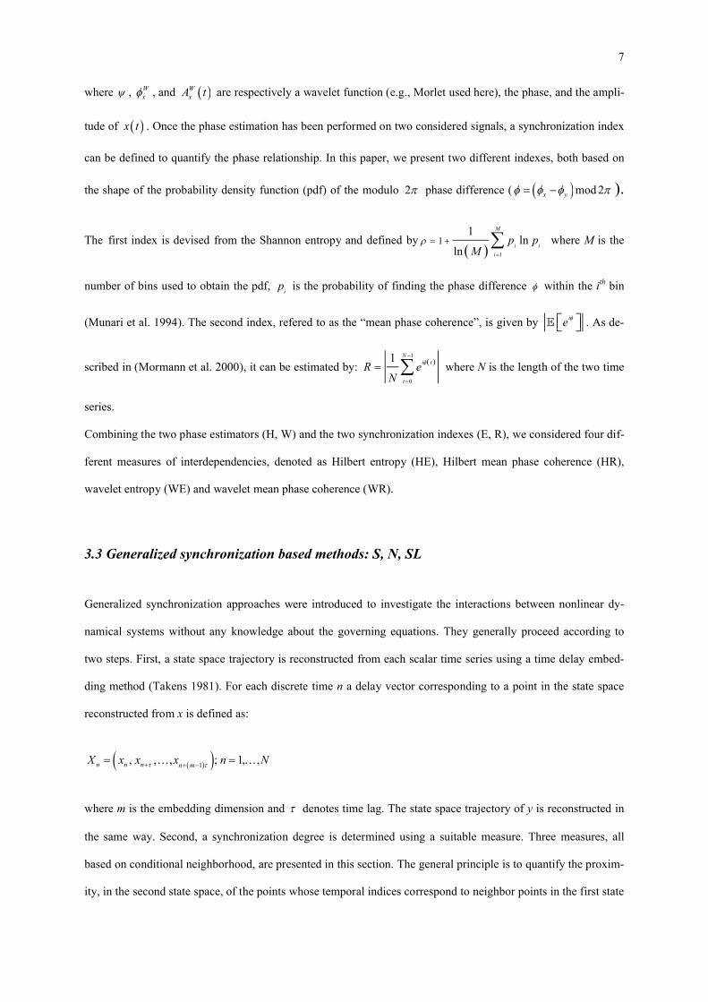
where , Wx , and W
xA t are respectively a wavelet function (e.g., Morlet used here), the phase, and the ampli-
tude of x t . Once the phase estimation has been performed on two considered signals, a synchronization index
can be defined to quantify the phase relationship. In this paper, we present two different indexes, both based on
the shape of the probability density function (pdf) of the modulo 2 phase difference ( mod 2x y ).
The first index is devised from the Shannon entropy and defined by 1
11
lnln
M
i i
i
p pM
where M is the
number of bins used to obtain the pdf, i
p is the probability of finding the phase difference within the ith bin
(Munari et al. 1994). The second index, refered to as the “mean phase coherence”, is given by ie . As de-
scribed in (Mormann et al. 2000), it can be estimated by: 1
0
1 Ni t
t
R eN
where N is the length of the two time
series.
Combining the two phase estimators (H, W) and the two synchronization indexes (E, R), we considered four dif-
ferent measures of interdependencies, denoted as Hilbert entropy (HE), Hilbert mean phase coherence (HR),
wavelet entropy (WE) and wavelet mean phase coherence (WR).
3.3 Generalized synchronization based methods: S, N, SL
Generalized synchronization approaches were introduced to investigate the interactions between nonlinear dy-
namical systems without any knowledge about the governing equations. They generally proceed according to
two steps. First, a state space trajectory is reconstructed from each scalar time series using a time delay embed-
ding method (Takens 1981). For each discrete time n a delay vector corresponding to a point in the state space
reconstructed from x is defined as:
1, , , ; 1, ,n n n n mX x x x n N
where m is the embedding dimension and denotes time lag. The state space trajectory of y is reconstructed in
the same way. Second, a synchronization degree is determined using a suitable measure. Three measures, all
based on conditional neighborhood, are presented in this section. The general principle is to quantify the proxim-
ity, in the second state space, of the points whose temporal indices correspond to neighbor points in the first state
8
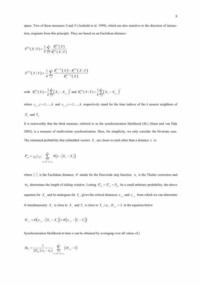
space. Two of these measures S and N (Arnhold et al. 1999), which are also sensitive to the direction of interac-
tion, originate from this principle. They are based on an Euclidean distance:
1
1|
|
kNk n
kn n
R XS X Y
N R X Y
1
11
|1|
N kNk n n
Nn n
R X R X YN X Y
N R X
with ,
2
1
1n j
kk
n n rj
R X X Xk
and ,
2
1
1|
n j
kk
n n sj
R X Y X Xk
where ,
, 1, ,n j
r j k and ,
, 1, ,n j
s j k respectively stand for the time indices of the k nearest neighbors of
nX and
nY .
It is noteworthy that the third measure, referred to as the synchronization likelihood (SL) (Stam and van Dijk
2002), is a measure of multivariate synchronization. Here, for simplicity, we only consider the bivariate case.
The estimated probability that embedded vectors n
X are closer to each other than a distance is:
2 1
1 2
1, 2( )
1
N
x n n jw wj
w n j w
P X X
where is the Euclidean distance; stands for the Heaviside step function, 1
w is the Theiler correction and
2w determines the length of sliding window. Letting , ,x n y n refP P P be a small arbitrary probability, the above
equation for n
X and its analogous for n
Y , gives the critical distances ,x n
and ,y n
from which we can determine
if simultaneously n
X is close to j
X and n
Y is close to j
Y , i.e.,,
2n j
H in the equation below
, , ,n j x n n j y n n jH X X Y Y
Synchronization likelihood at time n can be obtained by averaging over all values of j
1 2
,12 1
11
2
N
n n jjref
w n j w
SL HP w w

9
All aforementioned measures are normalized between 0 and 1; the 0 value means that the two signals are com-
pletely independent. On the opposite, the 1 value means that the two signals are completely synchronized.
Finally, in order to deal with the evolution, in time, of brain connectivity the three measures described above can
be estimated over a sliding window.
4. Model-based evaluation methodology
In order to perform an objective comparison of methods, we propose a model-based approach in which a priori
knowledge about the underlying relationship between systems that generate output signals is available. As illu-
strated in figure 1, connectivity methods are applied on the output signals X and Y produced by two models of
signal generation S1 and S2. The coupling between these two models can be adjusted using a coupling parameter
C. Some noise (N1 and N2) can be added to output signals. Evaluated methods provide a quantity Q (normalized
between 0 and 1) measured from X and Y and supposed to characterize the connectivity between the two models.
Therefore, this framework offers the possibility to study the behavior of candidate connectivity methods with re-
spect i) to the coupling parameter C, ii) to the type of model that is used to generate X and Y and iii) to the fea-
tures of noise present on output signals. In this context, the “ideal” method would provide a quantity Q which
would reflect any variation of coupling parameter C for any model of signal generation, with low bias and va-
riance and high sensitivity. This consideration led us to propose different models for generating outputs signals
(section 4.1) and three criteria (section 4.2) to evaluate the behavior of connectivity methods with respect to the
variation of parameter C.
4.1 Models of signal generation
Table 1 gives an overview of signal generation models used in this study. As depicted, these models can be di-
vided into three main families: i) models of coupled stochastic signals (M1 and M2), ii) models of coupled
nonlinear dynamical systems (M3 and M4) and iii) models of coupled neuronal populations (M5). In each fam-
ily, various situations were considered in order to check for the influence of signal properties (narrow versus
broad band activity) or the influence of noise on connectivity measures. The main characteristics of each model
are described hereafter.
4.1.1 Coupled broad band signals: M1

10
Model M1 generates two broad band signals ( 1 2,x x ) built using two independent and a common white noises
respectively (N1, N2) and (N3):
1 1 3
2 2 3
1
1
x C N CN
x C N CN
where 0 1C is the coupling degree; for 0C the signals are independent and for 1C they are identic-
al.
4.1.2 Coupled narrow band signals: M2(PR) and M2(AR)
In M2, two narrowband signals around a frequency 0
f are generated from four lowpass filtered white noises
(NF1, NF2, NF3, and NF4). They are combined in two ways in order to share either a phase relationship (PR) or
an amplitude relationship (AR), only:
1 1 0 1
2 2 0 1 2
1 1 0 1
2 1 2 0 2
cos 2:
cos 2 1
cos 2:
1 cos 2
x A f tPR
x A f t C C
x A f tAR
x CA C A f t
where 2 2
1 1 2A NF NF , 2 2
2 3 4A NF NF , 2
11 arctan NF
NF , 4
32 arctan NF
NF , and 0 1C . For 0C the
two signals have independent phase and amplitude and for 1C they have identical phase or amplitude.
We also used some nonlinear deterministic systems for modeling nonlinear synchronized coupled oscillators.
Here we report results obtained for two of them: Rössler-Rössler coupled system (M3) (Pikovsky et al. 1996) and
Hénon-Hénon coupled system (M4) (Bhattacharya 2001)
4.1.3 Coupled Rössler systems: M3
In M3 two Rössler systems (Rossler 1976) are coupled and the driver system is given by:
1
2 3
2
1 2
3
3 1
0.15
0.2 10
x
x
dxx x
dt
dxx x
dt
dxx x
dt

11
and the response system is described by:
1
2 3 1 1
2
1 2
3
3 1
0.15
0.2 10
y
y
dyy y C x y
dt
dyy y
dt
dyy y
dt
Here 0.95x
, 1.05y
, and C is the coupling degree.
4.1.4 Coupled Hénon systems: M4a and M4b
Hénon map (Hénon 1976) is a nonlinear deterministic which is discrete by construction. In model M4, we
make use of two of them to simulate a unidirectional coupled system. The driver system is given by:
21 1.4 1xx n x n b x n
and the response system is
21 1.4 1 1yy n cx n y n c y n b y n
where C is a coupling degree and 0.3x
b ; to create different situation, oncey
b is set to 0.3 to have two
identical systems (M4a) and once y
b is set to 0.1 to have two non-identical systems (M4b).
4.1.5 Coupled neuronal populations: M5
In order to simulate realistic temporal dynamics encountered in real depth-EEG signals, as recorded in patients
with drug-resistant epilepsy during pre-surgical evaluation, a physiologically-relevant computational model of
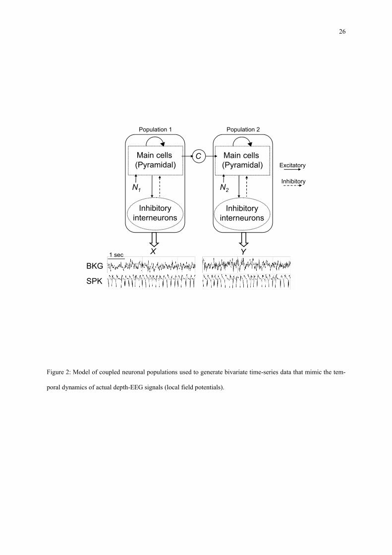
EEG generation was used. As illustrated in figure 2, this model represents the activity of two distant - and pos-
sibly coupled - neuronal populations. Each population generates a local field potential (X and Y) that can be seen
as a depth-EEG signal if one does not consider the source-electrode transfer function. Readers may refer to
(Wendling et al. 2000) for detailed description and generalization to more than 2 populations. In this model, each
population contains two subpopulations of neurons that mutually interact via excitatory or inhibitory feedback:
main pyramidal cells and local interneurons. The excitatory influence from non-specific afferents is modeled by
a Gaussian input noise (1
N or 2
N ) that globally represents the average density of afferent action potentials on
population 1 and population 2. Pyramidal cells are excitatory neurons that project their axons to distant areas of
12
the brain. The model accounts for this type of connection by using the average pulse density of action potentials
from the main cells of population 1 as an excitatory input to population 2. In addition, this uni-directional con-
nection from population 1 to population 2 is characterized by parameter C which represents the “synaptic gain”,
allowing for tuning the degree of coupling between the two populations. Other parameters include excitatory and
inhibitory gains in feedback loops as well as average number of synaptic contacts between subpopulations. The
model was used to generate two kinds of signals: background (BKG) and spiking (SPK) activity respectively ob-
tained for normal and increased excitation/inhibition ratio in each population. For both cases, bivariate data were
simulated. The normalized coupling parameter C was varied from 0 (independence between signals) to 1 (de-
pendence between signal, similar temporal dynamics).
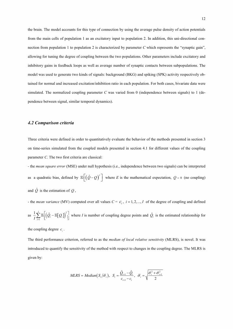
4.2 Comparison criteria
Three criteria were defined in order to quantitatively evaluate the behavior of the methods presented in section 3
on time-series simulated from the coupled models presented in section 4.1 for different values of the coupling
parameter C. The two first criteria are classical:
- the mean square error (MSE) under null hypothesis (i.e., independence between two signals) can be interpreted
as a quadratic bias, defined by 2
Q̂ Q where E is the mathematical expectation, 0Q (no coupling)
and Q̂ is the estimation of Q ,
- the mean variance (MV) computed over all values C = ic , 1, 2, ...,i I of the degree of coupling and defined
as 2
1
1 ˆI
i ii
Q QI
where I is number of coupling degree points and ˆiQ is the estimated relationship for
the coupling degree i
c .
The third performance criterion, referred to as the median of local relative sensitivity (MLRS), is novel. It was
introduced to quantify the sensitivity of the method with respect to changes in the coupling degree. The MLRS is
given by:
2 2
1 1
1
ˆ ˆ ˆ ˆ, ,
2i i i i
i i i ii i
Q QMLRS Median S S
c c

13
where i
S is the increase rate of the estimated relationship and i
is the square root of the average of estimated
variances associated to two adjacent values of the coupling degree. One can also use the median of the distribu-
tion of local relative sensitivity instead of its mean because the fluctuation in its estimation may make this distri-
bution very skewed.
Methods with lower values of MSE and MV can be considered to have better performances. Conversely, higher
MLRS values indicate better performances.
5. Results
For all models of signal generation (M1-M5) and for all values of parameter C (from 0 to 1 by steps of 0.1),
Monte Carlo simulations were performed in order to assess statistical properties of connectivity measures pro-
vided by methods described in section 3 and to comparatively evaluate their performances according to criteria
presented in section 4.2. To proceed, long duration time-series signals (200000 samples) sampled at 256 Hz were
generated using each model, for discrete values of the coupling parameter C, ranging from 0 to 1, by steps of
0.1. All quantities were estimated over a sliding window of 512 samples (2 seconds of activity) moving by steps
of 64 samples (75% overlapping) and then averaged over time. In GS methods, parameter was estimated as
follows. First the mutual information as a function of positive time lag was plotted and then, as described in
(Sills et al. 2000), time lag was chosen as the abscissa value corresponding to the first minimum this curve.
The embedded dimension m, in this family of methods, was determined from the Cao method (Cao 1997).
To limit the length of this section, we will only detail the results obtained in two cases (models M2(PR) and M5
(SPK)) and provide a global synthesis that summarizes the performances of the three families of methods in all
considered situations.
Results obtained in model M2 for phase relationship only (PR), are shown in figure 3. They show that phase syn-
chronization methods (HE, HR, WE, WR) exhibited higher performances than other methods, as it could be ex-
pected. Similarly, results obtained with R² and h² methods were correct. On the opposite, generalized synchroni-
zation methods and coherence (CF) had lower performances (S, SL: low sensitivity to C variation, S: strong bias,
SL: strong variance, CF: low sensitivity). Regarding the variance of estimation, it can be noticed that some me-
thods (R², WE) perform better than others. For higher coupling values, the variance decreases for all methods,
except SL.
14
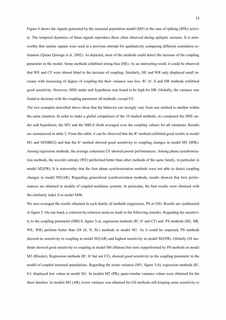
Figure 4 shows the signals generated by the neuronal population model (M5) in the case of spiking (SPK) activi-
ty. The temporal dynamics of these signals reproduce those often observed during epileptic seizures. It is note-
worthy that similar signals were used in a previous attempt for qualitatively comparing different correlation es-
timators (Quian Quiroga et al. 2002). As depicted, most of the methods could detect the increase of the coupling
parameter in the model. Some methods exhibited strong bias (HE). As an interesting result, it could be observed
that WE and CF were almost blind to the increase of coupling. Similarly, HE and WR only displayed small in-
crease with increasing of degree of coupling but their variance was low. R², h², S and HR methods exhibited
good sensitivity. However, MSE under null hypothesis was found to be high for HR. Globally, the variance was
found to decrease with the coupling parameter all methods, except CF.
The two examples described above show that the behavior can strongly vary from one method to another within
the same situation. In order to make a global comparison of the 10 studied methods, we computed the MSE un-
der null hypothesis, the MV and the MRLS (both averaged over the coupling values) for all situations. Results
are summarized in table 2. From this table, it can be observed that the R² method exhibited good results in model
M1 and M5(BKG) and that the h² method showed good sensitivity to coupling changes in model M5 (SPK).
Among regression methods, the average coherence CF showed poorer performances. Among phase synchroniza-
tion methods, the wavelet entropy (WE) performed better than other methods of the same family, in particular in
model M2(PR). It is noteworthy that the four phase synchronization methods were not able to detect coupling
changes in model M2(AR). Regarding generalized synchronization methods, results showed that best perfor-
mances are obtained in models of coupled nonlinear systems. In particular, the best results were obtained with
the similarity index S in model M4b.
We also averaged the results obtained in each family of methods (regression, PS or GS). Results are synthesized
in figure 5. On one hand, a criterion-by-criterion analysis leads to the following remarks. Regarding the sensitivi-
ty to the coupling parameter (MRLS, figure 5-a), regression methods (R², h² and CF) and PS methods (HE, HR,
WE, WR) perform better than GS (S, N, SL) methods in model M1. As it could be expected, PS methods
showed no sensitivity to coupling in model M2(AR) and highest sensitivity in model M2(PR). Globally GS me-
thods showed good sensitivity to coupling in model M4 (Hénon) but were outperformed by PS methods in model
M3 (Rössler). Regression methods (R², h² but not CF), showed good sensitivity to the coupling parameter in the
model of coupled neuronal populations. Regarding the mean variance (MV, figure 5-b), regression methods (R²,
h²) displayed low values in model M1. In models M2 (PR), quasi-similar variance values were obtained for the
three families. In models M2 (AR), lower variance was obtained for GS methods still keeping some sensitivity to

15
the coupling parameter. PS methods showed very low variance in model M3 (Rössler). In model M4 (Hénon),
GS methods exhibited the highest variance but were, in turn, the most sensitive to the coupling parameter. For
model M5, PS and regression methods performed better than GS methods. Regarding the mean square error un-
der null hypothesis (MSE, figure 5-c), results showed that some methods can be characterized by a high bias
value like GS methods in model M2, PS methods in model M3 and GS methods in model M5.
On the other hand, a model-by-model analysis of figure 5 shows that for model M1 regression methods perform
better than others as the MV is the lowest while the MRLS is the highest. For model M2 (in the case of PR), it is
evident that PS methods are the most appropriate. For model M2 (in the case of AR), there is no consensus for
the best method. For model M3, PS methods outperform others although they are characterized by higher MSE
values. For model M4 (considering the four situations), GS methods have the lowest MSE and PS methods have
the lowest MV. As far as the MRLS is concerned, these two groups of methods perform equally. Finally, for the
neuronal population model M5, regression methods outperform others in the case of normal background EEG ac-
tivity. For spiking epileptic-like activity, these methods, in addition to PS methods have also higher perfor-
mances than GS methods.
6. Discussion
Relevance in the field of brain research and progress with respect to already published studies
Numerous methods have been introduced to tackle the difficult problem of characterizing the statistical relation-
ship between signals without a priori knowledge about the nature of this relationship. In brain research, a num-
ber of methods have been proposed and/or used to study normal or pathological processes. Such methods play a
key role as they are supposed to provide important information regarding brain connectivity from electrophysio-
logical recordings.
During the ten past years, some efforts have been made for comparing methods but mainly qualitatively (David
et al. 2004; Quian Quiroga et al. 2002) and for particular applications (Mormann et al. 2005; Pereda et al. 2005).
In this paper, we presented three families of methods (regression, phase synchrony and general synchronization)
and we compared their performances on the basis of simulations produced by various models (including a neu-
rophysiologically-relevant one) in which a parameter can be tuned in order to adjust the coupling between two
“systems” from which output signals are generated. Through this model, we were able to study the relationship
between the coupling parameter in the models and the quantity actually measured on output signals using “con-
nectivity” methods.

16
In this regard, this approach differs from that of Schiff et al. (Schiff et al. 1996) who evaluated one method to
characterize dynamical interdependence (based on mutual nonlinear prediction) on both simulated (coupled iden-
tical and non identical chaotic systems) and real (activity of motoneurons within a spinal cord motoneuron pool)
data. It also differs from other evaluation studies which mainly focused on qualitative comparisons (David et al.
2004; Quian Quiroga et al. 2002) and for specific applications (Mormann et al. 2005; Pereda et al. 2005). In the
particular field of EEG analysis, the model of coupled neuronal populations is of particular relevance since it ge-
nerates realistic temporal dynamics. In this model, for background activity (that can be considered as a broad-
band random signal), we found that coherence and phase synchrony methods (except HR) were not sensitive to
the increase of the coupling parameter whereas regression methods (linear and nonlinear) exhibited better sensi-
tivity. This result may be explained by the fact that the interdependence between simulated signals is not entirely
determined by a phase relationship. This point is crucial since it illustrates the fact that the choice of the method
used to characterize the relationship between signals is critical and may lead to possible incorrect interpretation
of results obtained on EEG data.
In addition, as background activity can be recorded in epileptic patients during interictal periods, our results also
relate to those recently published by Morman et al. (Mormann et al. 2005) in the context of seizure prediction.
For thirty different measures obtained from univariate and bivariate approaches, authors evaluated their ability to
distinguish between the interictal period and the pre-seizure period (sensitivity and specificity of all measures
were compared using receiver-operating-characteristics). In both types of approach (and consequently for biva-
riate methods similar to those implemented in the present study) they also found that linear methods performed
equally good or even better than nonlinear methods.
Limitations of this study
In this report, results about the characterization of the direction of coupling were not dealt with. This difficult
issue has already been addressed in various reports. For instance, Quian Quiroga et al. (Quian Quiroga et al.
2002) quantitatively tested two interdependence measures on coupled nonlinear oscillators for their ability to de-
termine whether one the two systems drives the other. Other families of approaches where also developed to es-
timate directional properties of the relationship between signals while taking into account possible influences of
external sources (Gourevitch et al. 2006). According to these approaches, causality between two signals (in
Granger’s sense) is estimated based on the predictability of one signal from the immediate past of the other sig-
nal.

17
Besides, the methods evaluated in this study are independent from frequency. However, in some situation, it
might be crucial to take frequency into account. Indeed, frequency-independent methods may not be able to re-
veal some phenomena like a hypersynchronization in a narrow frequency band as sometimes observed at the on-
set of partial seizures. An example is illustrated in figure 6 which displays the depth-EEG signals recorded from
mesial temporal lobe structures in a patient candidate to surgery. As observed, the seizure onset is marked by the
appearance of a fast activity clearly localized in the time-frequency representations (figure 6-b) of the two depth-
EEG signals (figure 6-a). A “frequency-locking” phenomenon is revealed by the computation of the linear corre-
lation as the function of time and frequency (see methods in (Ansari-Asl et al. 2005)). As shown in figure 6-c, at
seizure onset, the two depth-EEG signals are correlated in a well-defined frequency sub-band (around 30 Hz).
More importantly, it should be noticed that time-independent methods (R² and h²) that showed relatively robust
in simulations do not show significant changes at seizure onset (figure 6-d and 6-e). As these methods apply on
broadband signals, they are unable to detect the increase of correlation occurring at a specific frequency.
Summary of the main findings
The main findings of this study can be summarized as follows: (i) some of the compared methods are insensitive
to the coupling parameter in the model; (ii) results are dependent on signal properties (broad band versus narrow
band); (iii) generally speaking, there is no universal method to deal with signal coupling, i.e., none of the studied
methods performed better than the other ones in all studied situations.
Nevertheless, we notice that simple methods like R² and h² methods showed to be sensitive to the coupling pa-
rameter in the model with average or good performances. Therefore, it might be reasonable to first apply these
“robust” regression methods in order to characterize brain connectivity before using more sophisticated methods
that require specific assumptions about the underlying model of relationship. In all cases, it is highly recom-
mended to compare the results obtained from different connectivity methods to get more reliable interpretation
of measured quantities with respect to underlying coupling. Following this idea, results suggest that some infor-
mation could be inferred about the nature of the relationship based on the comparison of indexes provided by the
different methods although the question of the physiological plausibility of the nature of the relationship will al-
ways remain.
In addition, some coupling phenomena might correspond to increased correlation between output signals, but in
one or several specific sub-band(s). In such cases, time-frequency methods may also be of help. In this category,
it should be reminded that a characterization of the relationship based on a “same frequency to same frequency”
approach can only reveal the linear component of this relationship. A more general approach would allow for the

18
computation of the correlation (in a wide sense) between signals filtered in different frequency sub-bands but
might also lead to additional difficulties in the interpretation of results.
References
Ansari-Asl, K., Bellanger, J. J., Bartolomei, F., Wendling, F., and Senhadji, L. (2005). "Time-frequency charac-terization of interdependencies in nonstationary signals: application to epileptic EEG." IEEE Trans Biomed Eng, 52(7), 1218-26.
Ansari-Asl, K., Senhadji, L., Bellanger, J. J., and Wendling, F. (2006). "Quantitative evaluation of linear and nonlinear methods characterizing interdependencies between brain signals." Phys Rev E Stat Nonlin Soft Matter Phys, 74(3 Pt 1), 031916.
Arnhold, J., Grassberger, P., Lehnertz, K., and Elger, C. E. (1999). "A robust method for detecting interdepend-ences: application to intracranially recorded EEG." Physica D: Nonlinear Phenomena, 134(4), 419-430.
Barlow, J. S., and Brazier, M. A. (1954). "A note on a correlator for electroencephalographic work." Electroen-cephalogr Clin Neurophysiol, 6(2), 321-5.
Bartolomei, F., Wendling, F., Bellanger, J. J., Regis, J., and Chauvel, P. (2001). "Neural networks involving the medial temporal structures in temporal lobe epilepsy." Clin Neurophysiol, 112(9), 1746-60.
Bendat, J., and Piersol, A. (1971). Random data: analysis and measurement procedures, Willey-Interscience.Bhattacharya, J. (2001). "Reduced degree of long-range phase synchrony in pathological human brain." Acta
Neurobiol Exp (Wars), 61(4), 309-18.Brazier, M. A. (1967). "Varieties of computer analysis of electrophysiological potentials." Electroencephalogr
Clin Neurophysiol, Suppl 26:1-8.Brazier, M. A. (1972). "Spread of seizure discharges in epilepsy: anatomical and electrophysiological considera-
tions." Exp Neurol, 36(2), 263-72.Brazier, M. A., and Casby, J. U. (1952). "Cross-correlation and autocorrelation studies of electroencephalo-
graphic potentials." Electroencephalogr Clin Neurophysiol, 4(2), 201-11.Cao, L. (1997). "Practical method for determining the minimum embedding dimension of a scalar time series."
Physica D: Nonlinear Phenomena, 110(1-2), 43-50.Cooley, J. W., and Tukey, J. W. (1965). "An Algorithm for the Machine Calculation of Complex Fourier Series."
Math. Comput., 19, 297-301.David, O., Cosmelli, D., and Friston, K. J. (2004). "Evaluation of different measures of functional connectivity
using a neural mass model." Neuroimage, 21(2), 659-73.Delprat, N., Escudie, B., Guillemain, P., Kronland-Martinet, R., Tchamitchian, P., and Torresani, B. (1992).
"Asymptotic wavelet and Gabor analysis: extraction of instantaneous frequencies." Information Theory, IEEE Transactions on, 38(2), 644-664.
Duckrow, R. B., and Spencer, S. S. (1992). "Regional coherence and the transfer of ictal activity during seizure onset in the medial temporal lobe." Electroencephalogr Clin Neurophysiol, 82(6), 415-22.
Franaszczuk, P. J., and Bergey, G. K. (1999). "An autoregressive method for the measurement of synchroniza-tion of interictal and ictal EEG signals." Biol Cybern, 81(1), 3-9.
Gotman, J. (1983). "Measurement of small time differences between EEG channels: method and application to epileptic seizure propagation." Electroencephalogr Clin Neurophysiol, 56(5), 501-14.
Gotman, J. (1987). "Interhemispheric interactions in seizures of focal onset: data from human intracranial re-cordings." Electroenceph. Clin. Neurophysiol, 67, 120-133.
Gourevitch, B., Bouquin-Jeannes, R. L., and Faucon, G. (2006). "Linear and nonlinear causality between signals: methods, examples and neurophysiological applications." Biol Cybern, 95(4), 349-69.
Haykin, S., Racine, R. J., Xu, Y., and Chapman, C. A. (1996). "Monitoring neural oscillation and signal trans-mission between cortical regions using time-frequency analysis of electroencephalographic activity." Proceedings of IEEE, 84, 1295-1301.
Hénon, M. (1976). "A two-dimensional mapping with a strange attractor." Communications in Mathematical Physics, 50, 69-77.
Iasemidis, L. D. (2003). "Epileptic seizure prediction and control." IEEE Trans Biomed Eng, 50(5), 549-58.Kalitzin, S. N., Parra, J., Velis, D. N., and Lopes da Silva, F. H. (2007). "Quantification of unidirectional nonlin-
ear associations between multidimensional signals." IEEE Trans Biomed Eng, 54(3), 454-61.

19
Ktonas, P. Y., and Mallart, R. (1991). "Estimation of time delay between EEG signals for epileptic focus local-ization: statistical error considerations." Electroencephalogr Clin Neurophysiol, 78(2), 105-10.
Le Van Quyen, M., Foucher, J., Lachaux, J., Rodriguez, E., Lutz, A., Martinerie, J., and Varela, F. J. (2001). "Comparison of Hilbert transform and wavelet methods for the analysis of neuronal synchrony." J Neu-rosci Methods, 111(2), 83-98.
Lehnertz, K. (1999). "Non-linear time series analysis of intracranial EEG recordings in patients with epilepsy--an overview." Int J Psychophysiol, 34(1), 45-52.
Lopes da Silva, F., Pijn, J. P., and Boeijinga, P. (1989). "Interdependence of EEG signals: linear vs. nonlinear associations and the significance of time delays and phase shifts." Brain Topogr, 2(1-2), 9-18.
Mars, N., and Lopes da Silva, F. (1983). "Propagation of seizure activity in kindled dogs." Electroencephalogra-phy and Clinical Neurophysiology, 56, 194-209.
Mormann, F., Kreuz, T., Rieke, C., Andrzejak, R. G., Kraskov, A., David, P., Elger, C. E., and Lehnertz, K. (2005). "On the predictability of epileptic seizures." Clin Neurophysiol, 116(3), 569-87.
Mormann, F., Lehnertz, K., David, P., and Elger, C. E. (2000). "Mean phase coherence as a measure for phase synchronization and
its application to the EEG of epilepsy patients." Physica. D, 144, 358-369.Munari, C., Tassi, L., Kahane, P., Francione, S., DiLeo, M., and Quarato, P. (1994). "Analysis of clinical symp-
tomatology during stereo-EEG recorded mesiotemporal lobe seizures." Epileptic seizures and syn-dromes, W. P, ed., John Libbey & Co, London.
Pereda, E., DelaCruz, D. M., DeVera, L., and Gonzalez, J. J. (2005). "Comparing Generalized and Phase Syn-chronization in Cardiovascular and Cardiorespiratory Signals." Biomedical Engineering, IEEE Transac-tions on, 52(4), 578-583.
Pijn, J. P. (1990). "Quantitative evaluation of EEG signals in epilepsy, nonlinear associations, time delays and nonlinear dynamics," University of Amsterdam, Amsterdam.
Pijn, J. P., and Lopes da silva, F. H. (1993). "Propagation of electrical activity: nonlinear associations and time delays between EEG signals." in Basic Mechanisms of the Eeg, Brain Dynamics, S. Zschocke and E. J. Speckmann, Eds. Boston: Birkhauser, 41-61.
Pikovsky, A., Rosenblum, M., and Kurths, J. (2001). "Synchronization : a universal concept in nonlinear sci-ences." Cambridge: Cambridge University Press.
Pikovsky, A. S., Rosenblum, M., and Kurths, J. (1996). "Synchronization in a population of globally coupled chaotic oscillators." Europhys. Lett., 34(3), 165-170.
Quian Quiroga, R., Kraskov, A., Kreuz, T., and Grassberger, P. (2002). "Performance of different synchroniza-tion measures in real data: a case study on electroencephalographic signals." Phys Rev E Stat Nonlin Soft Matter Phys, 65(4 Pt 1), 041903.
Rosenblum, M., Pikovsky, A., and Kurths, J. (2004). "Synchronization approach to analysis of biological sig-nals." Fluctuation Noise Lett., 4, L53-L62.
Rossler, O. E. (1976). "An equation for continuous chaos." Physics Letters A, 57(5), 397-398.Schiff, S. J., So, P., Chang, T., Burke, R. E., and Sauer, T. (1996). "Detecting dynamical interdependence and
generalized synchrony through mutual prediction in a neural ensemble." Physical Review. E. Statistical Physics, Plasmas, Fluids, and Related Interdisciplinary Topics, 54(6), 6708-6724.
Senhadji, L., Thoraval, L., and Carrault, G. (1996). "Continuous wavelet transform: ECG recognition based on phase and modulus representations and hidden Markov models." Wavelets in medicine and biology, A. Aldroubi and M. Unser, eds., CRC Press, NewYork, 439-463.
Sills, G. J., Leach, J. P., Kilpatrick, W. S., Fraser, C. M., Thompson, G. G., and Brodie, M. J. (2000). "Concen-tration-effect studies with topiramate on selected enzymes and intermediates of the GABA shunt." Epi-lepsia, 41 Suppl 1, S30-4.
Stam, C. J., and van Dijk, B. W. (2002). "Synchronization likelihood: an unbiased measure of generalized syn-chronization in multivariate data sets." Physica D: Nonlinear Phenomena, 163(3-4), 236-251.
Storm van Leeuwen, W., Arntz, A., Spoelstra, P., and Wieneke, G. H. (1976). "The use of computer analysis for diagnosis in routine electroencephalography." Rev Electroencephalogr Neurophysiol Clin, 6(2), 318-27.
Takens, F. (1981). "Lecture Nontes in Mathematics." Springer, 898, 366.Thatcher, R., Krause, P., and Hrybyk, M. (1986). "Cortico-cortical associations and EEG coherence: a two-
compartmental model." Electroenceph Clin Neurophysiol, 64(2), 123-143.Uhlhaas, P. J., and Singer, W. (2006). "Neural synchrony in brain disorders: relevance for cognitive dysfunctions
and pathophysiology." Neuron, 52(1), 155-68.Wendling, F., Bartolomei, F., Bellanger, J. J., and Chauvel, P. (2001a). "Interpretation of interdependencies in
epileptic signals using a macroscopic physiological model of the EEG." Clinical Neurophysiology, 112(7), 1201-1218.

20
Wendling, F., Bartolomei, F., Bellanger, J. J., and Chauvel, P. (2001b). "Interpretation of interdependencies in epileptic signals using a macroscopic physiological model of the EEG." Clin Neurophysiol, 112(7), 1201-18.
Wendling, F., Bellanger, J. J., Bartolomei, F., and Chauvel, P. (2000). "Relevance of nonlinear lumped-parameter models in the analysis of depth-EEG epileptic signals." Biol Cybern, 83(4), 367-78.

21
Captions
Table 1: Models of signal generation. Abbreviation SNR denotes “Signal-to-Noise Ratio”.
Table 2: Summary of results. For each model (horizontal: M1-M5) and for each studied method (vertical: R²-SL), the value of the mean square error (MSE) under null hypothesis (H0, i.e. no coupling), the mean variance (MV) and the median of local relative sensitivity (MLRS) were computed from simulated signals. Values hig-hlighted in grey color correspond to the “best performances’, i.e. lowest MSE, lowest MV and highest MLRS. In some cases, methods were found to be insensitive to the variations of the coupling parameter C in the models. In these cases, the three criteria are not applicable (N/A).
Figure 1: general model proposed to study the behavior of bivariate methods aimed at characterizing the connec-tivity between coupled systems (unidirectional coupling is tuned using parameter C) from output signals X and Y.
Figure 2: Model of coupled neuronal populations used to generate bivariate time-series data that mimic the tem-poral dynamics of actual depth-EEG signals (local field potentials).
Figure 3: Results obtained from model M2 in the case coupling parameter C induces a phase relationship onlybetween signals. (a) Example of simulated signals. (b) Estimated relationship (mean value of the estimated quan-tity Q(X,Y) over all realizations as a function of the coupling degree in the model). (c) Variance of estimation.
Figure 4: Results obtained from the neuronal population model in the case of epileptic EEG activity (sustained spiking activity as observed during ictal periods in epilepsy). (a) Example of simulated signals. (b) Estimated re-lationship (mean value of the estimated quantity Q(X,Y) over all realizations as a function of the coupling degree in the model). (c) Variance of estimation
Figure 5: A summary of the performances (according to quantitative criteria introduced in this study) of the three families of methods for all considered models of signal generation. For M2(AR), results obtained for phase syn-chronization methods are not represented since these methods were found to be insensitive w.r.t changes of the cou-pling parameter in this case (see table 2).
Figure 6: A “frequency-locking” phenomenon observed at the onset of seizure in a patient with medial temporal lobe epilepsy. a) depth-EEG recordings from medial structures (X(t) : hippocampus, Y(t) : entorhinal cortex) performed in a patient with mesial temporal lobe epilepsy. b) Time-frequency representation of the signal energy (spectrogram method computed using the short-term Fourier Transform -STFT- of signals X and Y). White ar-rows show the occurrence of a fast discharge (around 30 Hz) at seizure onset. c) Time- frequency representation of the linear relationship between signals X and Y. The method consists in the computation of the linear correla-tion coefficient between signals filtered in narrow sub-bands. Grey arrow shows that the linear correlation in-creases within the specific frequency sub-band corresponding to the fast activity. d, e) Results obtained from “standard” (i.e. frequency-independent) linear (R²(t)) and nonlinear (h²(t)) methods. Black arrows show that the “localized-in-frequency” correlation increase is not detected.

22
Models ofcoupled stochastic
signals
M1 Generation of broad band signals
M2
M2 (PR)
Generation of narrow band signals(Phase relationship only)
M2 (AR)
Generation of narrow band signals(Amplitude relationship only)
Models of coupled nonlinear dynamical
systems
M3Coupled Rössler systems.
Generation of deterministic signals
M4
M4a(SNR=inf
)
Coupled Hénon systems: identical systems. Generation of deterministic
signals
M4a(SNR=2)
Coupled Hénon systems: identical systems. Generation of deterministic
signals + additive noise
M4b(SNR=inf
)
Coupled Hénon systems: non-identical systems. Generation of determi-
nistic signals
M4b(SNR=2)
Coupled Hénon systems: non-identical systems. Generation of determi-
nistic signals + additive noise
Models of coupled neuronal populations M5
M5(BKG)
Generation of EEG signals(background activity)
M5(SPK)
Generation of EEG signals(Spiking activity)
Table 1: Models of signal generation. Abbreviation SNR denotes “Signal-to-Noise Ratio”.

Coupled stochasticSignals
Coupled nonlinear dynamical systems
Coupled neuronalpopulations
M1 M2 (PR) M2(AR) M3M4a
(SNR=inf)M4a
(SNR=2)M4b
(SNR=inf)M4b
(SNR=2)M5(SPK) M5(BKG)
Reg
ress
ion
R²MSE (H0) 0.12 76.42 0.2 109.55 0.28 0.22 0.26 0.22 63.17 1.54
MV 3.6 200.1 366.6 65.5 51.7 23.9 17.4 10.9 215.8 21.2MRLS 57.6 3.94 0.41 1.38 6.99 2.93 21.31 16.85 1.3 1.2
CFMSE (H0) 104.48 108.22 N/A 91.14 107.14 107.83 102.53 104.17 N/A N/A
MV 5.0 203.7 N/A 199.4 26.6 13.1 11.6 9.2 N/A N/AMRLS 56.4 1.3 N/A 2.20 5.68 1.94 17.17 9.41 N/A N/A
h²MSE (H0) 1.10 117.45 0.31 151.14 3.43 1.33 2.73 1.12 103.79 5.99
MV 3.7 161.10 274.8 60.4 42.0 23.3 21.5 11.8 205.0 22.6MRLS 35.6 4.06 0.36 0.98 6.91 0.56 20.62 16.42 1.0 1.1
Ph
ase
Syn
chro
niz
atio
n
HEMSE (H0) 4.98 23.11 N/A 63.82 8.09 6.87 6.00 5.69 28.75 N/A
MV 2.4 57.2 N/A 19.0 25.5 4.2 4.2 2.3 45.3 N/AMRLS 40.9 6.58 N/A 15.5 7.16 3.98 20.54 15.58 1.2 N/A
HRMSE (H0) 3.00 175.56 N/A 473.07 6.26 4.99 2.74 3.04 249.31 18.99
MV 8.8 206.7 N/A 10.1 49.6 28.0 17.9 14.8 217.5 65.5MRLS 42.5 6.5 N/A 8.87 6.79 4.77 21.45 15.38 1.2 0.7
WEMSE (H0) 10.54 20.48 N/A 76.47 13.01 13.27 12.98 12.76 N/A N/A
MV 1.5 29.4 N/A 6.3 20.1 3.3 3.1 1.7 N/A N/AMRLS 47.0 6.69 N/A 13.8 11.8 5.07 19.20 11.75 N/A N/A
WRMSE (H0) 8.78 113.65 N/A 161.50 68.97 65.79 62.26 64.22 53.39 N/A
MV 6.0 118.6 N/A 17.6 23.2 14.6 11.4 10.1 38.4 N/AMRLS 46.6 6.76 N/A 8.83 10.27 4.68 20.02 14.80 1.2 N/A
Gen
eral
ized
Syn
-ch
ron
izat
ion
SMSE (H0) 75.51 28.45 0.17 26.59 0.03 27.47 0.03 27.41 107.53 120.04
MV 2.8 58.1 74.6 48.8 20.8 6.6 1.2 4.7 183.7 44.1MRLS 31.1 2.23 0.84 6.91 19.40 10.26 31.51 18.03 0.9 0.05
NMSE (H0) 0.41 378.44 0.6 116.76 0.63 0.30 0.55 0.33 201.46 4.90
MV 5.0 120.5 142.3 68.4 12.5 1.36 8.4 13.4 501.1 60.1MRLS 29.0 3.02 0.60 3.46 25.42 15.70 12.32 17.04 0.4 0.9
SLMSE (H0) 4.28 115.25 0.31 8.50 4.18 4.47 3.83 3.74 41.32 6.16
MV 44.8 253.4 209.1 253.5 104.2 138.2 163.5 139.2 383.8 59.2MRLS 8.32 0.772 0.41 3.52 2.41 2.61 4.90 3.84 1.3 0.007
Table 2 : see Captions section for legend


C
NoiseN1
NoiseN2
Signal generation model S1
Signal generation model S2
X Y
0 ≤ C ≤ Cmax
0 ≤ Q( X, Y ) ≤ 10 ≤ Q( X, Y ) ≤ 1
?
Figure 1: general model proposed to study the behavior of bivariate methods aimed at characterizing the connec-
tivity between coupled systems (unidirectional coupling is tuned using parameter C) from output signals X and
Y.
26
CMain cells(Pyramidal)
Inhibitoryinterneurons
Main cells(Pyramidal)
Inhibitoryinterneurons
Population 1 Population 2
N1 N2
Excitatory
Inhibitory
X Y
BKG
SPK
1 sec
Figure 2: Model of coupled neuronal populations used to generate bivariate time-series data that mimic the tem-
poral dynamics of actual depth-EEG signals (local field potentials).

27
0
0,2
0,4
0,6
0,8
1
0 0,2 0,4 0,6 0,8 1
0
0,005
0,01
0,015
0,02
0,025
0,03
0,035
0,04
0 0,2 0,4 0,6 0,8 1
R²
CF
h²
HE
HR
WE
WR
S
N
SL
c) Mean varianceb) Estimated relationship
X
Y
a) Model M2 (PR)
2 s
Coupling parameter C Coupling parameter C
0
0,2
0,4
0,6
0,8
1
0 0,2 0,4 0,6 0,8 1
0
0,005
0,01
0,015
0,02
0,025
0,03
0,035
0,04
0 0,2 0,4 0,6 0,8 1
R²
CF
h²
HE
HR
WE
WR
S
N
SL
c) Mean varianceb) Estimated relationship
X
Y
a) Model M2 (PR)
2 s
Coupling parameter C Coupling parameter C
Figure 3: Results obtained from model M2 in the case coupling parameter C induces a phase relationship only
between signals. (a) Example of simulated signals. (b) Estimated relationship (mean value of the estimated quan-
tity Q(X,Y) over all realizations as a function of the coupling degree in the model). (c) Variance of estimation.

28
0
0,2
0,4
0,6
0,8
1
0 0,05 0,1 0,2 0,3 0,4 0,5 1
0
0,02
0,04
0,06
0,08
0,1
0 0,05 0,1 0,2 0,3 0,4 0,5 1
R²
CF
h²
HE
HR
WE
WR
S
N
SL
c) Mean variance
X
a) Model M5 (SPK)
Coupling parameter C Coupling parameter C
b) Estimated relationship
Y2 s
0
0,2
0,4
0,6
0,8
1
0 0,05 0,1 0,2 0,3 0,4 0,5 1
0
0,02
0,04
0,06
0,08
0,1
0 0,05 0,1 0,2 0,3 0,4 0,5 1
R²
CF
h²
HE
HR
WE
WR
S
N
SL
c) Mean variance
X
a) Model M5 (SPK)
Coupling parameter C Coupling parameter C
b) Estimated relationship
Y2 s
Figure 4: Results obtained from the neuronal population model in the case of epileptic EEG activity (sustained
spiking activity as observed during ictal periods in epilepsy). (a) Example of simulated signals. (b) Estimated re-
lationship (mean value of the estimated quantity Q(X,Y) over all realizations as a function of the coupling degree
in the model). (c) Variance of estimation

29
a)
b)
c)
0
10
20
30
40
50
60
M1
M2(PR)
M2(AR) M3
M4a(SNR=inf)
M4a(SNR=2)
M4b(SNR=inf)
M4b(SNR=2)
M5(BKG)
M5(SPK)
Regression
Phase Sync.
Generalized sync.
0
0,005
0,01
0,015
0,02
0,025
0,03
0,035
0,04
M1
M2(PR)
M2(AR)M3
M4a(SNR=inf)
M4a(SNR=2)
M4b(SNR=inf)
M4b(SNR=2)
M5(BKG)
M5(SPK)
Regression
Phase Sync.
Generalized sync.
0
0,05
0,1
0,15
0,2
0,25
M1
M2(PR)
M2(AR) M3
M4a(SNR=inf)
M4a(SNR=2)
M4b(SNR=inf)
M4b(SNR=2)
M5(BKG)
M5(SPK)
Regression
Phase Sync.
Generalized sync.
Ave
rage
dM
RLS
Ave
rage
dM
VA
vera
ged
MS
E
Figure 5: A summary of the performances (according to quantitative criteria introduced in this study) of the three
families of methods for all considered models of signal generation. For M2(AR), results obtained for phase syn-
chronization methods are not represented since these methods were found to be insensitive w.r.t changes of the
coupling parameter in this case (see table 2).

30
Hippocampus
Entorhinal cortex
X(t)
Y(t)
0
max
0
1
STFT(X)
STFT(Y)
R² (t, f)
Seizure onset
1.0
.75
0.5
.25
0
1.0
.75
0.5
.25
0
120
90
60
30
0120
90
60
30
0120
90
60
30
0
R²(t)
h² (t)X Y
h² (t)Y X
5 s
Freq. (Hz)
Freq. (Hz)
Freq. (Hz)
a)
b)
c)
d)
e)
Hippocampus
Entorhinal cortex
X(t)
Y(t)
0
max
0
1
STFT(X)
STFT(Y)
R² (t, f)
Seizure onset
1.0
.75
0.5
.25
0
1.0
.75
0.5
.25
0
120
90
60
30
0
120
90
60
30
0120
90
60
30
0
120
90
60
30
0120
90
60
30
0
120
90
60
30
0
R²(t)
h² (t)X Yh² (t)X Y
h² (t)Y Xh² (t)Y X
5 s
Freq. (Hz)
Freq. (Hz)
Freq. (Hz)
a)
b)
c)
d)
e)
Figure 6: a “frequency-locking” phenomenon observed at the onset of seizure in a patient with medial temporal
lobe epilepsy. a) depth-EEG recordings from medial structures (X(t) : hippocampus, Y(t) : entorhinal cortex)
performed in a patient with mesial temporal lobe epilepsy. b) Time-frequency representation of the signal energy
(spectrogram method computed using the short-term Fourier Transform -STFT- of signals X and Y). White ar-
rows show the occurrence of a fast discharge (around 30 Hz) at seizure onset. c) Time- frequency representation
of the linear relationship between signals X and Y. The method consists in the computation of the linear correla-
tion coefficient between signals filtered in narrow sub-bands. Grey arrow shows that the linear correlation in-
creases within the specific frequency sub-band corresponding to the fast activity. d, e) Results obtained from
“standard” (i.e. frequency-independent) linear (R²(t)) and nonlinear (h²(t)) methods. Black arrows show that the
“localized-in-frequency” correlation increase is not detected.