From BOP to BOSS and Beyond: Time Series

Classification with Dictionary Based Classifiers

James Large1, Anthony Bagnall1 Simon Malinowski2

Romain Tavenard3

1School of Computing SciencesUniversity of East Anglia

United Kingdomajb@uea.ac.uk

2 University of Rennes 1,3 University of Rennes 2France

Abstract

A family of algorithms for time series classification (TSC) involve run-ning a sliding window across each series, discretising the window to forma word, forming a histogram of word counts over the dictionary, thenconstructing a classifier on the histograms. A recent evaluation of twoof this type of algorithm, Bag of Patterns (BOP) and Bag of SymbolicFourier Approximation Symbols (BOSS) found a significant difference inaccuracy between these seemingly similar algorithms. We investigate thisphenomenon by deconstructing the classifiers and measuring the relativeimportance of the four key components between BOP and BOSS. Wefind that whilst ensembling is a key component for both algorithms, theeffect of the other components is mixed and more complex. We concludethat BOSS represents the state of the art for dictionary based TSC. BothBOP and BOSS can be classed as bag of words approaches. These areparticularly popular in Computer Vision for tasks such as image classifica-tion. Converting approaches from vision requires careful engineering. Weadapt three techniques used in Computer Vision for TSC: Scale InvariantFeature Transform; Spatial Pyramids; and Histrogram Intersection. Wefind that using Spatial Pyramids in conjunction with BOSS (SP) producesa significantly more accurate classifier. SP is significantly more accuratethan standard benchmarks and the original BOSS algorithm. It is notsignificantly worse than the best shapelet based approach, and is onlyoutperformed by HIVE-COTE, an ensemble that includes BOSS as aconstituent module.

1

arX

iv:1

809.

0675

1v1

[cs

.LG

] 1

8 Se

p 20

18

1 Introduction

A family of algorithms for time series classification involve constructing a dic-tionary of words from the set of time series then forming a bag of words overthat dictionary for each of the time series. More specifically, they run a slidingwindow across each series, discretise the window to form a word, form a his-togram of word counts over the dictionary, then constructing a classifier on thehistograms. A recent evaluation of two of this type of algorithm, Bag of Patterns(BOP) and Bag of Symbolic Fourier Approximation Symbols (BOSS) found asignificant difference in accuracy between these seemingly similar algorithms.We investigate this phenomena by deconstructing the classifiers and measuringthe relative importance of the four key differences between BOP and BOSS. Wefind that ensembling makes both approaches significantly more accurate, butthe effect of the other three components is more complex.

Both BOP and BOSS can be classed as bag of words approaches. These areparticularly popular in Computer Vision for tasks such as image classification.Converting approaches for 2-D image classification to 1-D series classificationfrom a range of domains requires careful engineering. We adapt three techniquesused in Computer Vision for TSC: Scale Invariant Feature Transform; SpatialPyramids; and Histrogram Intersection. We find that using Spatial Pyramids inconjunction with BOSS (SP) produces a significantly more accurate classifier. SPis significantly more accurate than standard benchmarks and the original BOSSalgorithm. It is not significantly worse than the best shapelet based approach,and is only outperformed by HIVE-COTE, an ensemble that includes BOSS asa constituent module.

The rest of this document is structured as follows. Section 2 provides anoverview of the broad range of TSC algorithms, whereas Section 3 gives moredetail into dictionary based approaches. We provide an overview of the ComputerVision framework for bag of words classification in Section 4. Section 5 presentsthe results of our deconstruction of BOP and BOSS and Section 6 describes ourevaluation of enhancements to BOSS. We conclude with Section 7.

2 TSC Background

A recent experimental study [2] compared and evaluated a diverse set of twentyTSC algorithms that have been published in leading journals and conferences inthe last five years. They proposed the following taxonomy of algorithms.

2.1 Algorithms based on raw series

Techniques based on raw series compare two series either as a vector (as withtraditional classification) or by a distance measure that uses all data points.In the latter case, measures are typically combined with one-nearest-neighbour(1-NN) classifiers and the simplest variant is to compare series using EuclideanDistance. However, this baseline is easily beaten in practice, and most research

2

effort has been directed toward finding techniques that can compensate forsmall misalignments between series using specialised elastic distance measures.The almost universal benchmark for whole series measures is Dynamic TimeWarping (DTW) but numerous alternatives have been proposed. The mostaccurate whole series approach (according to the bakeoff comparison [2]) is theElastic Ensemble (EE) [19], an ensemble of 1-NN classifiers using various elasticmeasures, including DTW, combined through a proportional voting scheme.

2.2 Interval-based algorithms

Rather than use the raw series, the interval class of algorithm select one or morephase-dependent intervals of the series. At its simplest, this involves a featureselection of a contiguous subset of attributes. However, the three most effectivetechniques generate multiple intervals, each of which is processed and forms thebasis of a member of an ensemble classifier [10, 6, 5]. There is no significantdifference in accuracy between these approaches, and the simplest is the TimeSeries Forest (TSF) [10].

2.3 Shapelet-based algorithms

Shapelet approaches are a family of algorithms that focus on finding shortpatterns that define a class and can appear anywhere in the series. A class isdistinguished by the presence or absence of one or more shapelets somewherein the whole series. Shapelets were first introduced in [27]. The two leadingways of finding shapelets are through enumerating the candidate shapelets in thetraining set [20, 14] or searching the space of all possible shapelets with a form ofgradient descent [13]. The bakeoff found that the shapelet transform algorithmused in conjunction with a heterogeneous classifier ensemble (ST-HESCA) is themost accurate approach on average.

2.4 Dictionary-based algorithms

Shapelet algorithms look for subseries patterns that identify a class throughpresence or absence. However, if a class is defined by the relative frequencyof a pattern, shapelet approaches will be poor. Dictionary approaches addressthis by forming frequency counts of repeated patterns. They approximate andreduce the dimensionality of series by transforming into representative words,then compute similarity by comparing the distribution of words. Three of theapproaches that have been published in the data mining literature are: Bagof Patterns (BOP) [18]; the Symbolic Aggregate Approximation Vector SpaceModel (SAXVSM) [26]; and the Bag of Symbolic Fourier Approximation Symbols(BOSS) [24]. We provide an overview of these algorithms in Section 3.

3

2.5 Spectral-based algorithms

The frequency domain will often contain discriminatory information that is hardto detect in the time domain. Methods include constructing an autoregressivemodel ([8, 1]) or combinations of autocorrelation, partial autocorrelation andautoregressive features ([3]). An interval based spectral ensemble called RandomInterval Spectral Ensemble (RISE) was proposed in [21] and shown to be moreaccurate on average than whole series spectral approaches.

2.6 Combinations

Two or more of the above approaches can be combined into a single classifier.For example, an approach that concatenates different feature spaces is describedin [15], forward selection of features for a linear classifier is the method adoptedin [11]) and transformation into a feature space that represents each group andensembling classifiers together formed the basis of the Flat-COTE classifier [3].A modular meta-ensemble of classifiers from each class of algorithms (EE, TSF,BOSS, ST-HESCA and RISE) called HIVE-COTE is currently the state of theart classifier for TSC when evaluated on the UCR/UEA data and simulatedproblems [21]. However, on individual problems, there is a wide variation betweenthe classifiers, and the ensemble is not always the best approach. The nature ofthe discriminatory features will dictate the best class of algorithm.

Our basic assumption is that dictionary classifiers will be best for problemswhere classes are defined by the frequency of occurrence of a shape in each seriesrather than its binary presence or absence. For example, suppose data containsshort sine waves that repeat at random intervals. In one class there are manyrepeating patterns, in another class there are few. Figure 1 gives example of thiskind of data.

A whole series and an interval approach will fail because the positioning of therepeating patterns is random. Shapelets will not detect this phenomena becausethey look for the presence or absence of a pattern. Spectral approaches maydo better, but not if there are large intervals between the signals. A dictionaryapproach should be able to detect that one pattern occurs more frequently inone class than the other. Our objective here is to develop the best dictionarybased TSC algorithm.

We describe the state of the art by summarising previously published, freelyavailable and reproducible results1. We compare the relative performance of threebase line classifiers: rotation forest with 50 trees (RotF); 1-NN with Euclideandistance (Euclid); DTW with window set through cross validation (DTW), arepresentative of each class of algorithm: EE, TSF, ST and RISE, the threedictionary classifiers BOP, SAXVSM and BOSS and two ensemble approaches,Flat-COTE and HIVE-COTE.

To compare multiple classifiers on multiple problems, following the recom-mendation of Demsar [9], we use the Friedmann test to determine if there wereany statistically significant differences in the rankings of the classifiers. However,

1see www.timeseriesclassification.com for details

4

(a) (b)

Figure 1: Two examples of simulated dictionary data. with a mixture of truncatedhead and shoulders and sine shapelets. Figure (a) has low noise and Figure (b)has standard white noise.121110 9 8 7 6 5 4 3 2 1

2.3471 HIVE−COTE3.1176 Flat−COTE4.4882 ST−HESCA5.1529 BOSS6.0824 EE6.3412 TSF6.5353RISE

7.1294RotF

8.1824DTW

9.1235SAXVSM

9.4353BoP

10.0647Euclid

Figure 2: Average ranks of 12 classifiers on 100 resamples of 85 data sets. Theresults were first presented in [2] and [22]. A solid bar across a set of classifiersindicates there is no significant difference within that group.

following recent recommendations in [7] and [12], we have abandoned the Ne-menyi post-hoc test originally used by [9] to form cliques (groups of classifierswithin which there is no significant difference in ranks). Instead, we compareall classifiers with pairwise Wilcoxon signed rank tests, and form cliques usingthe Holm correction (which adjusts family-wise error less conservatively than aBonferroni adjustment).

5

HIVE-COTE is the most accurate algorithm over all, but features of these re-sults excited our interest about dictionary classifiers. Firstly, BOP and SAXVSMperformed very poorly. Neither is significantly better than 1-NN Euclidean dis-tance and neither could beat the benchmark classifiers rotation forest and DTW.In stark contrast, BOSS is one of the best performers. It is not significantly worsethan the ST-HESCA and only beaten by the two meta ensembles Flat-COTEand HIVE-COTE. HIVE-COTE contains BOSS whereas Flat-COTE does not,and the fact that HIVE-COTE is significantly better than Flat-COTE is furtherevidence in support of BOSS. On a head to head comparison, BOSS beats BOPon 80 of the 85 datasets. The mean difference in accuracy is over 8%. Thesealgorithms are seemingly similar, so why is BOSS so much better than BOP?Answering this question requires a more in depth understanding of how thesealgorithms work.

3 Dictionary Based Algorithms

Dictionary based algorithms share the same basic structure. In summary, awindow of length w is passed across each series. Each subseries is then representedby some string or pattern that is representative of it. In the cases considered here,each subseries from the windowing is first compressed from length w to l. Theshortened subseries are then discretised, so that each of the l data is restrictedto one of α values. The occurrence of the resulting ‘word’, r, is recorded in ahistogram, although in a stage called numerosity reduction, contiguous series ofidentical words are counted as a single occurrence. Each series has a separatehistogram (also referred to as bag), and new instances are classified based onthe distance between their own histogram and those in the training set, basedby default on 1-nearest neighbour classification, though other methods could beused.

There are four key stages at which major differences between dictionarybased algorithms may arise:

1. the compression method to get from w real valued data to l real valueddata;

2. the discretisation technique used to convert the l real valued data into ldiscrete data with α possible values;

3. the methods of representing the collections of transformed subseries; and

4. the distance measure used to compare histograms and/or the classificationalgorithm used to classify new cases.

3.1 Bag of Patterns (BOP) [18]

BOP (described in Algorithm 1) is a dictionary classifier built on the SymbolicAggregate Approximation (SAX) [17] algorithm. SAX reduces w to l throughPiecewise Aggregate Approximation (PAA) (i.e. each of the l new points is an

6

average over an interval length w/l) and discretises to α values using quantilesof the normal distribution. If consecutive windows produce identical words,then only the first of that run is recorded. This is included to avoid the overcounting of trivial matches, especially in smooth regions of the originating series.The distribution of words over a series forms a count histogram. To classifynew samples, the same transform is applied to the new series and the nearestneighbour histogram within the training matrix found. BOP sets the threeparameters through cross validation on the training data.

Algorithm 1 buildClassifierBOP(A list of n cases of length m, T = (X,y))

Parameters: the word length l, the alphabet size α and the window length w1: Let H be a list of n histograms (h1, . . . ,hn)2: p← ∅3: for i← 1 to n do4: for j ← 1 to m− w + 1 do5: q← xi,j . . . xi,j+w−16: r← SAX(q, l, α)7: if r 6= p then8: pos ← index(r) {the function index determines the location of the

word r in the count matrix hi}9: hi,pos ← hi,pos + 1

10: p← r

The Symbolic Aggregate Approximation - Vector Space Model (SAXVSM) [26]combines the SAX representation used in BOP with the Vector Space Modelcommonly used in Information Retrieval. The key differences between BOPand SAXVSM is that SAXVSM forms word distributions over classes ratherthan series and weights these by the term frequency/inverse document frequency(tf · idf). For SAXVSM, term frequency tf refers to the number of times a wordappears in a class and document frequency df means the number of classes aword appears in. tf · idf is then defined as

tfidf(tf, df) =

{log (1 + tf) · log( c

df ) if df > 0

0 otherwise

where c is the number of classes. There is no significant difference in accuracybetween BOP and SAXVSM, so we can without loss of generality restrict ourattention to BOP.

3.2 Bag of Symbolic Fourier Approximation Symbols (BOSS) [24]

BOSS also uses windows to form words over series, and represents them ina simple histogram format, but it has several major differences to BOP andSAXVSM. BOSS uses a truncated Discrete Fourier Transform (DFT) insteadof a PAA on each window. Another difference is that the truncated seriesis discretised through a technique called Multiple Coefficient Binning (MCB),

7

rather than using fixed intervals. MCB finds the discretising break points as apreprocessing step by estimating the distribution of the Fourier coefficients. Thisis performed by segmenting the series into disjoint windows, performing a DFT,then finding breakpoints for each coefficient such that each bin contains the samenumber of elements. The whole process of forming words is called SymbolicFourier Approximation (SFA). BOSS then involves similar stages to BOP; itwindows each series to form the term frequency through the application of DFTand discretisation by MCB, performs numerosity reduction, and forms histogramsof the words in each series. A bespoke distance function is used for nearestneighbour classification. This non symmetrical function only includes distancesbetween frequencies of words that actually occur within the first histogrampassed as an argument, which refers to the test case.

Another major difference is that BOSS forms an ensemble by retaining allclassifiers with training accuracy within 92% of the best during the parametersearch of window sizes. New instances are classified by a majority vote of theresulting ensemble. Algorithm 2 details the construction of histograms for agiven parameter set.

Algorithm 2 buildClassifierBOSS(A list of n cases of length m, T = (X,y))

Parameters: the word length l, the alphabet size α, the window length w,normalisation parameter p

1: Let H be a list of n histograms (h1, . . . ,hn)2: Let B be a matrix of l by α breakpoints found by MCB3: p← ∅4: for i← 1 to n do5: for j ← 1 to m− w + 1 do6: s← xi,j . . . xi,j+w−17: q← DFT(s, l, α,p) { q is a vector of the complex DFT coefficients}8: q′ ← (q1 . . . ql/2)9: r← MCB(q′,B)

10: if r 6= p then11: pos←index(r)12: hi,pos ← hi,pos + 113: p← r

In a manner reminiscent of the way SAXVSM adapts BOP, BOSS-VectorSpace (BOSS-VS) [25] modifies BOSS to form class histograms rather thaninstance histograms. Switching to class histograms massively reduces the memoryrequirements and speeds up classification, but it has no significant effect onaccuracy, unless it is to reduce it (see the results in [25]). In this work we areconcerned with classification accuracy. The questions we address are, firstly, whyis BOSS so much better than BOP (see Section 5) and secondly, can we refineBOSS to make it more accurate (see Section 6).

8

4 Computer Vision Bag of Words Framework

The histogram approach used by dictionary classifiers has similarities to manyapproaches used in the field of Computer Vision. A typical Computer Visionbag of words framework involves the following stages:

1. extraction of keypoints;

2. description of keypoints;

3. bag forming; and

4. classification based on bags.

BOP and BOSS extract keypoints through sliding a window over the whole series,reducing the size of the number of keypoints through numerosity reduction and arestriction of window sizes. However, approaches for dictionary based TSC morein line with the Computer Vision approach have been proposed. [4] describes anapproach for using Scale Invariant Feature Transform (SIFT) [23] features foruse in TSC with dictionary classifiers. We describe this approach in detail inSection 4.1 and have implemented a version in the WEKA based TSC codebase2.

We also consider a common technique in Computer Vision called SpatialPyramids, proposed in [16] and described in Section 4.2. We try incorporatingthis as a wrapper for BOSS. It could equally be applied to other dictionaryapproaches.

A more complex Computer Vision approach applied to TSC is proposedin [28]. This involves a combined approach of peak finding and hybrid samplingto extract keypoints, using Histogram of Oriented Gradients (HOG-1D) andDynamic Time Warping-Multidimensional Scaling (DTW-MDS) to form featuresdescribing the keypoints, clustering them with a K component Gaussian MixtureModel, forming bags based on Fisher Vector encoding and finally constructing alinear kernel Support Vector Machine classifier. The resulting classifier, calledHOG-1D+DTW-MDS, is evaluated on the standard single folds of 43 of theUEA/UCR data sets. They do not compare the results of HOG-1D+DTW-MDS to the published results for BOSS, presumably due to the lag time inpublication. Using the results in Table 3 from [28] and the BOSS results presentedin [2], we find no significant difference between HOG-1D+DTW-MDS and BOSS(HOG-1D+DTW-MDS wins on 22, BOSS on 19 and they tie on 2).

4.1 Bag of Temporal SIFT Words (BOTSW) Classifier

The Bag of Temporal SIFT Words (BOTSW) algorithm [4] adopts a versionof the Computer Vision bag of words framework that is easier to reproducethan that described in [28], not least because the C++ source code is publiclyavailable3. BOTSW first extracts keypoints from every time series through

2https://bitbucket.org/TonyBagnall/time-series-classification3https://github.com/a-bailly/dbotsw

9

regular sampling at a rate r, which is a parameter of the method. Then, eachkeypoint is described by ns feature vectors, where ns is the number of consideredscales. Each feature vector describes the keypoint at a particular scale. Toobtain the feature vector of a keypoint at a scale s, the time series is filtered bya Gaussian filter of width s. nb blocks of size α are selected around the keypoint.Gradients of the filtered time series are computed for every point of every blockand then weighted by a Gaussian function to give greater importance to thosepoints nearer to the keypoint.

Each block is described by two values: the sum of positive gradients inthe block and the sum of negative gradients. A feature vector that describesa keypoint at a particular scale is a 2nb-long vector. A dictionary of featurevectors is learned by a k-means clustering on the whole set of feature vectorsfrom the time series database. Feature vectors are then quantized using thedictionary. The number of occurrences of these words in the series is computedto form a histogram, which is normalised using Signed Square Root (SSR) then l2normalisation. This nomalized histogram is the final feature vector representingthis series.

In [4], a Support Vector Machine was used to classify feature vectors. However,our objective is to assess the utility of the SIFT features in relation to the BOSSfeatures. Hence, to minimize the differences between BOSS and BOP we use 1NNclassification. The parameters nb in {4, 8, 12, 16, 20}, α in {4, 8}, and k in {32,64, 128, 256, 512, 1024} are tuned through a grid search with cross validation. Tofurther align with BOSS, we form an ensemble of BOTSW classifiers, retainingall parameter sets with training accuracy within 92% of the global maximum.This homogeneous ensemble classifies new instances with a simple majority vote.

4.2 BOSS Ensemble with Spatial Pyramids (SP)

The essence of dictionary classifiers is to ignore temporal information throughconsideration of the recurrence of short subseries. Whilst this will lead togood results in problem domains with repeated discriminatory features, thedisadvantage is that in some domains the location in time of a pattern is asimportant as the pattern itself. Spatial pyramids [16] are a method commonlyused in Computer Vision, which will allow us combine temporal and phaseindependent features. When applied to time series, using a spatial pyramidinvolves recursively segmenting each series and constructing histograms on thesegments.

Starting from the initial histogram across the whole series, histograms onsubsections are formed by repeatedly dividing the series L times. These his-tograms are weighted by 1

2L−l , which is inversely proportional to the level l atwhich they are found. All histograms are then combined and normalised to forma single elongated histogram feature.

Because of the weighting, similarity between features found at smaller divi-sions on the series have a more significant effect than those found on a moreglobal scale, as their temporal location becomes increasingly dissimilar. It isalso worth noting that a pyramid with one level is equivalent to the basic bag of

10

words, as no division has occurred.Since BOSS ensembles over different window sizes so that discriminatory

patterns of different lengths can all be accounted for, we search for L foreach member of the ensemble during training. An overview of the ensembleconstruction is given in Algorithm 3. Feature sets formed from an optimal wordlength, found through CV, for a given window size are generated as usual. Thisfeature set, implicitly produced as a pyramid with L = 1, is then augmentedand further CV is performed to find the optimal L in {1,2,3}. This effectivelydefines whether the discriminatory feature type described by this parameterset is more local or global in nature. If the training accuracy of the best wordlength and number of levels for this window size falls within 92% of the best, itis included in the ensemble. In classification, for each member the test instanceis transformed into a spatial pyramid using that member‘s parameters, and theclass of the train pyramid with the maximal Histogram Intersection or minimalBOSS Distance is returned. Figure 3 gives an example of the process of forminghistograms for SP.

Algorithm 3 buildBOSSEnsembleSP(A list of n cases of length m, T = {X,y})1: α = 42: featureSets = [features, trainAccuracies]3: for w in windowLengths() do4: bestWindowFeatureSet = null5: bestWindowAcc = 06: for k in wordLengths() do7: featureSet = BOSSTransform(w,k,α)8: acc = CrossValidate(featureSet)9: if acc > bestWindowAcc then

10: bestWindowAcc = acc, bestWindowFeatureSet = featureSet11: for L in 2,3 do12: featureSet = buildPyramid(bestWindowFeatureSet, L)13: acc = CrossValidate(featureSet)14: if acc > bestWindowAcc then15: bestWindowAcc = acc, bestWindowFeatureSet = featureSet16: featureSets.add(bestWindowFeatureSet, bestWindowAcc)17: maxWindowAcc = max(featureSets.trainAccuracies)18: for set in featureSets do19: if bestWindowAcc > maxWindowAcc*0.92 then20: addToEnsemble(set)

While computing the pyramids is very fast relative to the original productionof the SFA words, the additional space complexity is a concern for large datasetsas the final elongated histograms will be

∑L−1l=0 2l times larger. This can be

heavily mitigated by using sparse data representations, since histograms at higherlevels will be more sparse than those at lower levels. However, a cap of 100 wasalso placed on the maximum size of the ensemble to keep the space requirements

11

Figure 3: A series from the BeetleFly dataset, being divided at successive levelswith Bags of SFA words being formed for each subsection. H1...7 are combinedto form the final feature vector.

more reasonable. Thus if λ is the number of feature sets within the threshold ofthe max accuracy, the size of the final ensemble is min(100, λ).

4.3 Histogram Intersection (HI) Distance

A core task in any bag of words/dictionary based technique is to compare thedifferences between the resulting histograms in order to define class membership.BOP uses Euclidean Distance, SAX-VSM uses Cosine Similarity, and BOSSits own measure which is a slight alteration to Euclidean. We also test theHistogram Intersection similarity measure described in [16] which is used inmany different applications involving histograms. For a dictionary and resultinghistogram size of k, this is defined as:

HI(a,b) =

k∑i=1

min(ai, bi)

5 From BOP to BOSS

We perform all experiments using 77 of the datasets at the University of Califor-nia, Riverside/University of East Anglia (UCR/UEA) time series classificationrepository4 ([2]). There are 8 datasets that we do not use for practical reasons:their size means the classifiers take too long to train or require too much memoryto complete given our time frame and the number of experiments and resamplingperformed. The full list of problems we used is given in Table 4. Our focus is onbridging the accuracy gap between the two classifiers; optimizing for speed andmemory are of course very important, but are not the focus of this study. All ofour code and data is available from a public code repository and accompanyingwebsite5. We compare classifiers by the accuracy average over 25 stratifiedresamples (with the same train/test size of the original data).

4UCR/UEA TSC Repository: www.timeseriesclassification.com5www.timeseriesclassification.com/dami2017.php

12

Both BOP and BOSS tune their parameters through a leave one out crossvalidation on the train data for a predefined parameter space. The results forBOSS and BOP presented in [2] were obtained using the parameter space definedin the original papers, and these parameter spaces are different. To alleviate thispossible source of bias we have altered the BOP search space to match that ofBOSS (see Table 1). In a pairwise comparison between the BOP on the old andnew parameter space, the latter had higher average accuracy on 44 datasets andworse on 33. There is no significant difference between the old and new versions,and we conclude that we cannot explain the difference between BOP and BOSSon this factor.

Table 1: Parameter search spaces for BOP and BOSS.Algorithm Parameters

BOP published parameter search space w = 15%. . . 36% of ml = powers of 2 up to w/2

α = 2. . . 8BOSS published parameter search space w = 10. . . m

This space is used for both BOSS and BOP l = 8, 10, 12, 14, 16α = 4

BOP and BOSS are identical except for four features.

1. The window approximation method. Each window of length w isreduced to a series of length l through an approximation method. BOPuses Piecewise Aggregate Approximation whereas BOSS uses the truncatedFourier terms.

2. The discretisation method. Each value in the approximate series oflength l is discretised into one of α values. BOP uses the fixed intervalsdefined in SAX whereas BOSS uses the data driven technique MultipleCoefficient Binning (MCB).

3. The distance measure. BOP uses 1-NN with Euclidean distance whereasBOSS uses a 1-NN with a bespoke, non-symmetric distance function thatignores zero entries in the test histogram.

4. The classifier. BOSS is an ensemble of multiple transforms with differentparameters, whereas BOP is a single classifier.

To quantify the source of the difference in BOP and BOSS, we assess therelative importance of each of these components by adding each of the fourBOSS features into BOP. We then measure their importance to BOSS by inturn replacing each BOSS feature with that used in BOP. This gives us the 10BOP/BOSS variants listed in Table 2.

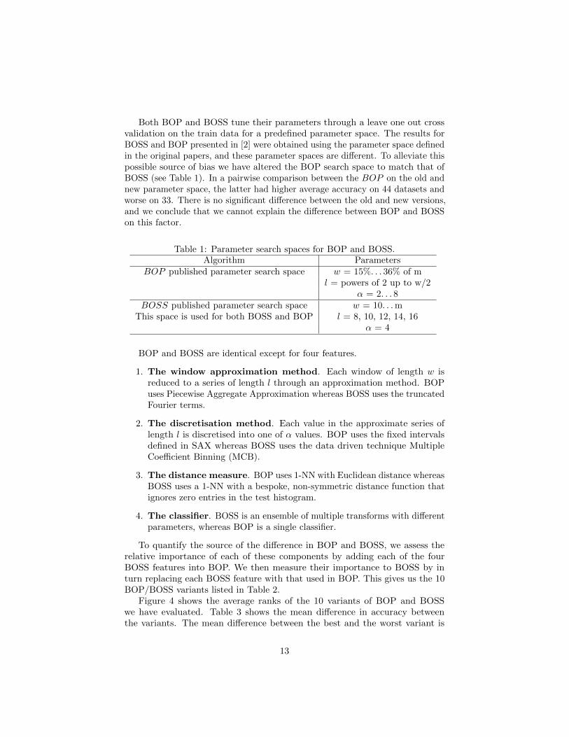
Figure 4 shows the average ranks of the 10 variants of BOP and BOSSwe have evaluated. Table 3 shows the mean difference in accuracy betweenthe variants. The mean difference between the best and the worst variant is

13

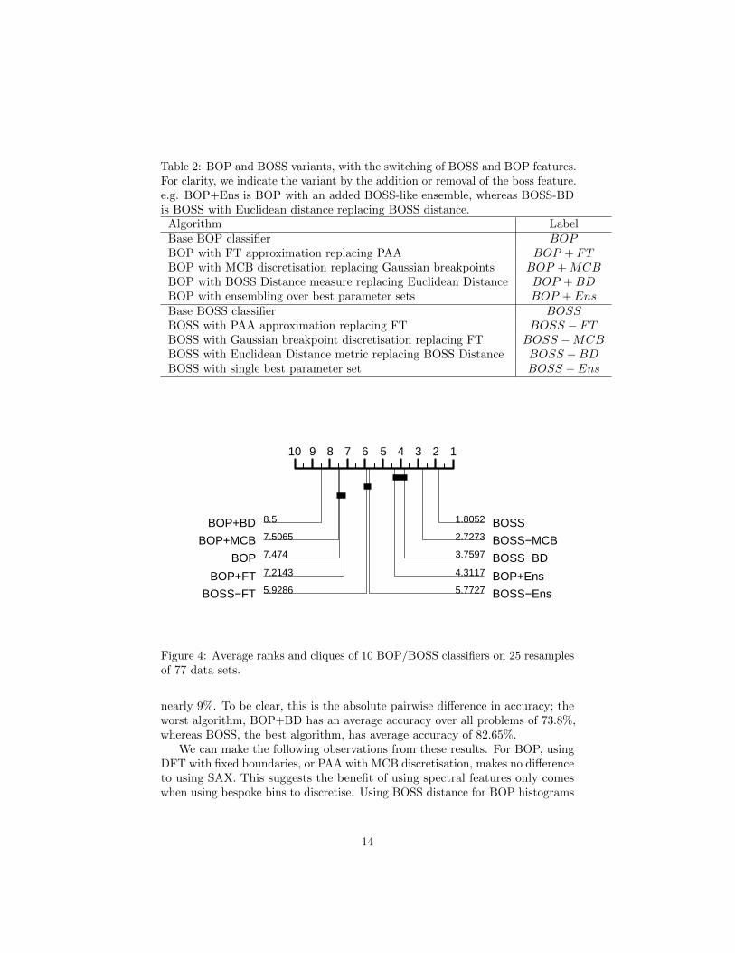
Table 2: BOP and BOSS variants, with the switching of BOSS and BOP features.For clarity, we indicate the variant by the addition or removal of the boss feature.e.g. BOP+Ens is BOP with an added BOSS-like ensemble, whereas BOSS-BDis BOSS with Euclidean distance replacing BOSS distance.

Algorithm LabelBase BOP classifier BOPBOP with FT approximation replacing PAA BOP + FTBOP with MCB discretisation replacing Gaussian breakpoints BOP +MCBBOP with BOSS Distance measure replacing Euclidean Distance BOP +BDBOP with ensembling over best parameter sets BOP + EnsBase BOSS classifier BOSSBOSS with PAA approximation replacing FT BOSS − FTBOSS with Gaussian breakpoint discretisation replacing FT BOSS −MCBBOSS with Euclidean Distance metric replacing BOSS Distance BOSS −BDBOSS with single best parameter set BOSS − Ens

10 9 8 7 6 5 4 3 2 1

1.8052 BOSS2.7273 BOSS−MCB3.7597 BOSS−BD4.3117 BOP+Ens5.7727 BOSS−Ens5.9286BOSS−FT

7.2143BOP+FT

7.474BOP

7.5065BOP+MCB

8.5BOP+BD

Figure 4: Average ranks and cliques of 10 BOP/BOSS classifiers on 25 resamplesof 77 data sets.

nearly 9%. To be clear, this is the absolute pairwise difference in accuracy; theworst algorithm, BOP+BD has an average accuracy over all problems of 73.8%,whereas BOSS, the best algorithm, has average accuracy of 82.65%.

We can make the following observations from these results. For BOP, usingDFT with fixed boundaries, or PAA with MCB discretisation, makes no differenceto using SAX. This suggests the benefit of using spectral features only comeswhen using bespoke bins to discretise. Using BOSS distance for BOP histograms

14

Table 3: The mean difference in accuracy between BOP and BOSS variants over77 datasets.

BOP+BD BOP+MCB BOP BOP+FT BOSS-FT BOSS-Ens BOP+Ens BOSS-BD BOSS-MCB BOSSBOP+BD 0.00% -0.97% -0.97% -0.71% -3.10% -3.61% -4.94% -5.59% -7.60% -8.88%

BOP+MCB 0.97% 0.00% -0.01% 0.26% -2.13% -2.65% -3.97% -4.62% -6.63% -7.91%BOP 0.97% 0.01% 0.00% 0.26% -2.12% -2.64% -3.96% -4.61% -6.63% -7.91%

BOP+FT 0.71% -0.26% -0.26% 0.00% -2.39% -2.90% -4.23% -4.88% -6.89% -8.17%BOSS-FT 3.10% 2.13% 2.12% 2.39% 0.00% -0.51% -1.84% -2.49% -4.50% -5.78%BOSS-Ens 3.61% 2.65% 2.64% 2.90% 0.51% 0.00% -1.32% -1.98% -3.99% -5.27%BOP+Ens 4.94% 3.97% 3.96% 4.23% 1.84% 1.32% 0.00% -0.65% -2.66% -3.94%BOSS-BD 5.59% 4.62% 4.61% 4.88% 2.49% 1.98% 0.65% 0.00% -2.01% -3.29%

BOSS-MCB 7.60% 6.63% 6.63% 6.89% 4.50% 3.99% 2.66% 2.01% 0.00% -1.28%BOSS 8.88% 7.91% 7.91% 8.17% 5.78% 5.27% 3.94% 3.29% 1.28% 0.00%

actually makes BOP significantly worse. The only component of BOSS thatsignificantly improves BOP is ensembling. This actually makes BOP significantlybetter than a single version of BOSS (the mean difference 1.32%). However,BOP ensemble is still significantly worse than the BOSS ensemble. Hence wecannot attribute the difference to the ensembling method alone: removing anyone of the four components of BOSS makes it significantly worse. The worstchange to make is to switch from DFT features to PAA features. This surprisedus, as we had assumed removing ensembling would cause the most harm. Clearlythe four features of BOSS that differentiate it from BOP are all required and allinteract to produce a better classifier. This highlights that the engineering ofalgorithms is often not linear, and components can interact in ways that maynot be intuitively obvious. This is most clearly observable when comparing theeffect of using the BOSS Distance (BD): BD makes BOP significantly worse butBOSS significantly better.

There is some difference in the structures of the resulting histograms of eachtransform which BOSS Distance is able to leverage over Euclidean Distancein the case of BOSS, but not BOP. Considering the actual bagging process isessentially the same between the two - both extract words from a massivelysparse space, and both use numerosity reduction - such an apparently clear, orrather ‘usable’, distinction in the final histograms is striking. BOSS Distanceignores words that do not appear in the test histogram, so for BOP these missingwords are seemingly informative, however for BOSS they are noise and removingthem is beneficial. Exactly why this is so is unclear. We suspect this differenceis due to the action of MCB, which creates a data driven discretisation. If theunderlying distribution diverges significantly from normality, MCB will create amore accurate representation and will hence capture an underlying pattern moreaccurately. This could lead to the truly informative words being separated fromthe uninformative noise more successfully, and so the words that are ignored aremore likely to be noise. This is just conjecture. Further work and analysis ofthe resulting histograms would need to be performed to fully understand themechanisms at work here, however this is beyond the scope of this work.

From these experiments we conclude that BOSS, as described in [24], rep-resents the state of the art for dictionary classifiers that were first introducedin [18]. Our next question is, can we improve on the state of the art?

15

6 BOSS Extensions

In Section 4 we described two approaches from Computer Vision that mayimprove dictionary classifiers: SIFT features [23], adapted for time series asdescribed in [4] and Spatial Pyramids [16] that have not formerly been used in thiscontext. We also described the Histogram Intersection as an alternative distancemeasure between histograms. We wish to assess whether adding these alternativestructures to the state of the art dictionary classifier gives an overall improvementin accuracy. To try and isolate the causes of any observed differences we startwith BOSS as the base classifier and make the minimum adjustments.

SPBD is a spatial pyramid built on top of the standard BOSS ensemble (usingBD). SPHI is a spatial pyramid built on top of BOSS, using histogram intersection.BOTSWBD is a bag of temporal-sift classifiers that use BD, whereas BOTSWHI

uses histogram intersection. All four classifiers ensemble in an identical way toBOSS (retain all models within 92% of the best), and each pair of classifiers (i.e.BOTSWBD/BOTSWHI and SPBD/SPHI) search identical parameter spaces.The average ranks and cliques are shown in Figure 5. The two SIFT basedclassifiers are significantly worse than BOSS, there is no significant differencebetween BOSS and SPBD, but SPHI is significantly better than BOSS.

5 4 3 2 1

2.2353 SPHI

2.4412 SPBD

2.875 BOSS

3.3676BOTSWBD

4.0809BOTSWHI

Figure 5: Average ranks and cliques for five variants of dictionary classifiers.

SPHI represents an advance for dictionary based algorithms for TSC, butwe do not wish to over sell the importance. Although SPHI wins on 51 of the77 problems, that actual differences are small. Figure 6 shows the scatter plotof accuracies of SPHI against BOSS. The results are fairly tightly grouped onthe line of equality. The overall mean difference in accuracy is just 0.64%. Wewould expect the improvements from SPHI to be apparent on problems wherediscriminatory features are phase dependent. For example, SPHI is over 7%more accurate than BOSS on WordSynonyms and 6% better on FiftyWords.The elastic ensemble is the most accurate classifier on these two problems, whichindicate the discriminatory features are time dependent. Conversely, SPHI is 6%worse than BOSS on ShapeletSim and 3.5% worse on SonyAIBORobotSurface1.The phase independent classifier ST-HESCA is the most accurate classifier for

16

these datasets, whereas EE does poorly. This indicates that the setting of theparameter L, like all parameters, is vulnerable to overfitting. Whereas it wouldhave evidently been better to use the regular BOSS classifier (or equivalentlysetting L=1 in the SP) on those latter datasets due to their phase-independentnature, in terms of training accuracy the parameter search process found someerroneous advantage to using more levels.

0.2

0.4

0.6

0.8

1

0.2 0.4 0.6 0.8 1

Me

an

SP

-HI

Te

st A

ccu

racy

Mean BOSS Test Accuracy

BOSS

Better Here

SP-HI

Better Here

0.2

0.4

0.6

0.8

1.0

0.2 0.4 0.6 0.8 1.0

Mean ST-HESCA Test Accuracy

ST-HESCA

Better Here

EE

Better Here

Figure 6: Scatter plot of accuracies for (a) SPHI vs BOSS and (b) EE vs ST-HESCA. The latter is provided to demonstrate the type of spread observable onthis data for two very different classifiers.

4 3 2 1

1.539 HIVE−COTE2.461 ST−HESCA2.5519SP−HI

3.4481CNN

Figure 7: A comparison of SP-HI to three alternative TSC approaches that arenot dictionary based.

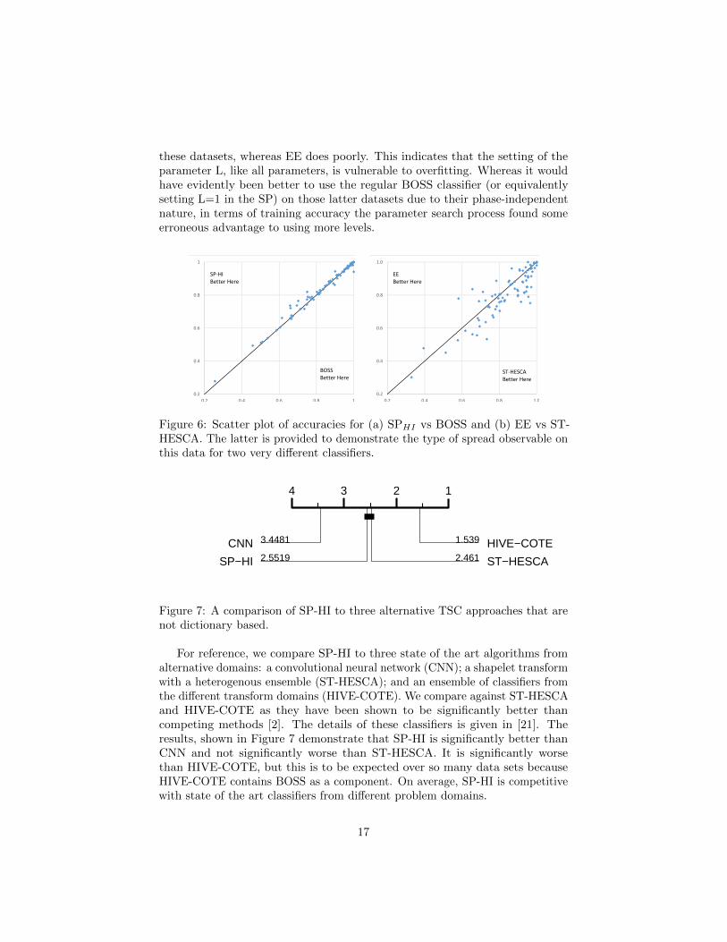
For reference, we compare SP-HI to three state of the art algorithms fromalternative domains: a convolutional neural network (CNN); a shapelet transformwith a heterogenous ensemble (ST-HESCA); and an ensemble of classifiers fromthe different transform domains (HIVE-COTE). We compare against ST-HESCAand HIVE-COTE as they have been shown to be significantly better thancompeting methods [2]. The details of these classifiers is given in [21]. Theresults, shown in Figure 7 demonstrate that SP-HI is significantly better thanCNN and not significantly worse than ST-HESCA. It is significantly worsethan HIVE-COTE, but this is to be expected over so many data sets becauseHIVE-COTE contains BOSS as a component. On average, SP-HI is competitivewith state of the art classifiers from different problem domains.

17

Table 4: The mean accuracy of five variants of dictionary classifiers. BOSS [24],spatial pyramid BOSS with histogram intersection distance (SP-HI) and BOSSdistance (SP-BD) and an adapted version of bag of temporal words [4] withhistogram intersection distance (BOTSW-BD) and BOSS distance (BOTSW-HI)

DataSet BOSS SP-HI SP-BD BOTSW-BD BOTSW-HIAdiac 74.94 (±0.15) 74.38 (±0.25) 74.77 (±0.26) 71.62 (±0.4) 71.59 (±0.29)ArrowHead 87.52 (±0.33) 88.66 (±0.67) 87.89 (±0.67) 87.36 (±0.58) 86.33 (±0.69)Beef 61.5 (±0.88) 66.13 (±1.49) 65.2 (±1.63) 54.93 (±1.61) 55.6 (±1.62)BeetleFly 94.85 (±0.57) 94.2 (±1.31) 93.6 (±1.28) 91.6 (±0.95) 92.8 (±1.04)BirdChicken 98.4 (±0.36) 97.8 (±1.04) 98 (±0.87) 95.2 (±0.84) 92.2 (±1.39)Car 85.5 (±0.45) 85.93 (±0.91) 85.8 (±1.01) 90.33 (±0.77) 88.2 (±0.71)CBF 99.81 (±0.04) 99.93 (±0.02) 99.91 (±0.03) 99.88 (±0.05) 99.85 (±0.07)ChlorineConcentration 65.96 (±0.13) 65.96 (±0.29) 65.97 (±0.31) 56.8 (±4.02) 58.67 (±11.73)CinCECGtorso 90.05 (±0.48) 94.39 (±0.77) 93.51 (±0.87) 78.24 (±0.95) 71.72 (±0.81)Coffee 98.86 (±0.2) 98.57 (±0.36) 98.57 (±0.36) 98.29 (±0.51) 98.71 (±0.41)Computers 80.23 (±0.23) 81.92 (±0.68) 81.54 (±0.54) 67.66 (±0.66) 65.55 (±0.51)CricketX 76.36 (±0.2) 78.53 (±0.42) 77.96 (±0.4) 81.22 (±0.43) 79.85 (±0.46)CricketY 74.93 (±0.18) 77.31 (±0.32) 76.98 (±0.41) 78.61 (±0.29) 77.04 (±0.47)CricketZ 77.57 (±0.19) 78.88 (±0.39) 78.51 (±0.35) 82.63 (±0.31) 82 (±0.46)DiatomSizeReduction 93.94 (±0.42) 93.93 (±0.65) 94.21 (±0.68) 91.19 (±0.68) 90.99 (±0.7)DistalPhalanxOC 81.46 (±0.21) 80.52 (±0.57) 81.25 (±0.56) 77.61 (±0.48) 76.09 (±14.59)DistalPhalanxOAG 81.41 (±0.28) 81.5 (±0.63) 81.24 (±0.6) 77.44 (±0.68) 77.29 (±0.72)DistalPhalanxTW 67.3 (±0.21) 67.34 (±0.45) 67.14 (±0.43) 65.06 (±0.41) 65.78 (±0.5)Earthquakes 74.59 (±0.04) 74.33 (±0.12) 74.76 (±0.04) 74.45 (±0.12) 74.82 (±0.15)ECG200 89.05 (±0.3) 87.04 (±0.64) 87.96 (±0.63) 86.96 (±0.55) 86.76 (±0.59)ECGFiveDays 98.33 (±0.28) 99.3 (±0.23) 99.21 (±0.24) 99.67 (±0.23) 99.33 (±0.31)FaceFour 99.56 (±0.1) 98.09 (±0.35) 98.14 (±0.35) 93.95 (±0.53) 91.59 (±0.83)FacesUCR 95.06 (±0.07) 95.62 (±0.15) 95.67 (±0.15) 95.31 (±0.1) 94.38 (±0.16)FiftyWords 70.22 (±0.16) 76.5 (±0.28) 76.9 (±0.3) 75.94 (±0.38) 72.32 (±0.24)Fish 96.87 (±0.11) 97.1 (±0.23) 96.96 (±0.25) 94.38 (±0.3) 95.36 (±0.26)GunPoint 99.41 (±0.11) 99.84 (±0.06) 99.73 (±0.1) 98.88 (±0.13) 98.75 (±0.1)Ham 83.6 (±0.38) 83.47 (±0.85) 83.62 (±0.86) 77.26 (±1.03) 76.15 (±1.15)Haptics 45.87 (±0.36) 49.36 (±0.74) 47.42 (±0.67) 47.04 (±0.56) 48.05 (±0.72)Herring 60.53 (±0.52) 60.44 (±1.17) 59.13 (±1.04) 60.94 (±1.32) 59.94 (±1.04)InlineSkate 50.26 (±0.35) 51.08 (±0.62) 51.4 (±0.59) 42.49 (±0.44) 40.92 (±0.65)InsectWingbeatSound 51.03 (±0.21) 51.67 (±0.43) 51.82 (±0.49) 50.34 (±0.27) 46.58 (±0.31)ItalyPowerDemand 86.6 (±0.36) 88.22 (±0.57) 87.14 (±0.86) 93.43 (±0.3) 92.96 (±0.31)LargeKitchenAppliances 83.66 (±0.19) 83.7 (±0.6) 82.02 (±0.5) 79.16 (±13.71) 78.24 (±0.29)Lightning2 81 (±0.46) 80.59 (±0.97) 80.2 (±0.93) 79.93 (±0.86) 79.21 (±1.04)Lightning7 66.56 (±0.54) 67.67 (±1.02) 68.33 (±1.05) 73.53 (±0.78) 71.07 (±0.78)Mallat 94.85 (±0.12) 94.8 (±0.24) 94.8 (±0.24) 89.35 (±0.5) 89.44 (±0.35)Meat 98.03 (±0.24) 98.33 (±0.47) 98.27 (±0.48) 95.87 (±0.67) 96.6 (±0.61)MedicalImages 71.46 (±0.23) 71.59 (±0.32) 72.19 (±0.33) 75.02 (±0.29) 72.87 (±0.27)MiddlePhalanxOC 80.82 (±0.19) 80.52 (±0.4) 80.78 (±0.36) 75.86 (±0.4) 75.6 (±14.8)MiddlePhalanxOAG 66.6 (±0.33) 65.58 (±0.67) 65.84 (±0.64) 61.3 (±0.56) 60.52 (±0.67)MiddlePhalanxTW 53.74 (±0.27) 53.87 (±0.49) 53.51 (±0.55) 53.61 (±0.43) 53.4 (±0.47)MoteStrain 84.6 (±0.31) 85.49 (±0.72) 85.33 (±0.62) 90.06 (±0.45) 89.28 (±0.59)OliveOil 87 (±0.41) 87.47 (±0.78) 87.47 (±0.78) 86.67 (±0.72) 86.93 (±0.94)OSULeaf 96.74 (±0.1) 97.79 (±0.14) 97.36 (±0.12) 87.4 (±0.42) 85.54 (±0.52)Phoneme 25.62 (±0.27) 27.84 (±0.41) 27.51 (±0.47) 21.85 (±0.34) 18.2 (±0.31)Plane 99.79 (±0.04) 99.89 (±0.06) 99.81 (±0.08) 99.54 (±0.1) 99.16 (±0.17)ProximalPhalanxOC 86.74 (±0.17) 86.89 (±0.29) 86.83 (±0.32) 79.82 (±0.37) 79.23 (±12.11)ProximalPhalanxOAG 81.9 (±0.22) 83 (±0.31) 82.85 (±0.38) 83 (±0.44) 82.79 (±0.46)ProximalPhalanxTW 77.28 (±0.22) 77.62 (±0.43) 77.48 (±0.39) 75.32 (±0.4) 75.3 (±0.34)RefrigerationDevices 78.46 (±0.37) 77.26 (±1.29) 77.28 (±1.25) 57.33 (±11.5) 67.34 (±0.83)ScreenType 58.6 (±0.3) 58.69 (±0.85) 58.56 (±0.67) 51.66 (±0.73) 45.57 (±0.67)ShapeletSim 100 (±0) 94.09 (±0.52) 100 (±0) 99.98 (±0.02) 98.91 (±0.23)SmallKitchenAppliances 75.02 (±0.42) 81.92 (±0.41) 77.74 (±0.71) 67.07 (±13.14) 62.28 (±6.74)SonyAIBORobotSurface1 89.74 (±0.43) 86.22 (±0.92) 89.36 (±1.12) 89.26 (±0.74) 86 (±0.97)SonyAIBORobotSurface2 88.77 (±0.31) 89.52 (±0.51) 88.04 (±0.55) 88.21 (±0.57) 86.06 (±0.71)SwedishLeaf 91.77 (±0.09) 92.51 (±0.17) 92.26 (±0.22) 89.08 (±14.55) 89.21 (±13.63)Symbols 96.12 (±0.15) 96.47 (±0.21) 96.25 (±0.23) 97.06 (±0.23) 96.23 (±0.31)SyntheticControl 96.79 (±0.09) 96.15 (±0.21) 96.68 (±0.16) 99.53 (±0.07) 98.68 (±0.14)ToeSegmentation1 92.88 (±0.3) 91.88 (±0.6) 92.44 (±0.63) 93.98 (±0.34) 91.58 (±0.56)ToeSegmentation2 95.97 (±0.18) 96.03 (±0.29) 96.15 (±0.32) 97.08 (±0.21) 95.75 (±0.32)Trace 99.99 (±0.01) 100 (±0) 100 (±0) 100 (±0) 100 (±0)TwoLeadECG 98.45 (±0.14) 98.65 (±0.24) 98.54 (±0.25) 97.23 (±0.32) 96.6 (±0.33)UWaveGestureLibraryY 66.12 (±0.11) 72.09 (±0.3) 71.79 (±0.26) 71.75 (±14.35) 69.67 (±13.34)Wine 91.17 (±0.63) 90.07 (±1.39) 90.07 (±1.4) 83.41 (±1.71) 84.74 (±1.79)WordSynonyms 65.88 (±0.19) 73.62 (±0.31) 73.47 (±0.34) 72.03 (±0.28) 68.56 (±0.38)Worms 73.49 (±0.45) 71.64 (±0.77) 72.42 (±1.05) 72.16 (±0.78) 72.31 (±0.88)WormsTwoClass 80.97 (±0.43) 80.62 (±0.92) 80.62 (±0.89) 79.74 (±0.78) 78.23 (±0.83)Yoga 90.99 (±0.13) 91.89 (±0.32) 91.52 (±0.34) 88.86 (±3.63) 88.71 (±0.21)wins 16 26.75 8.25 15.25 1.25

18

7 Conclusions

Dictionary classifiers are an important class of TSC algorithm that explicitlyuse the frequency of occurrence of repeating patterns as classification features.A previous study observed a huge difference in accuracy between two prominentapproaches, BOP [18] and BOSS [24]. In order to investigate why this is so, weidentify the four key differences between the two algorithms and assess theirimportance to both BOP and BOSS. We find that only one of these features,ensembling over different parameter values, is beneficial to both BOSS and BOP.Ensembling has proven successful in other domains for TSC [3], and it carriesno train time overhead if a parameter search is being conducted. BOP with anensemble is significantly better than a single BOSS classifier. Hence, we wouldrecommend anyone assessing a new TSC algorithm attempt to ensemble, notleast to make a better comparison to the state of the art. For example, it is quitepossible that HOG-1D+DTW-MDS [28] would be significantly more accurate ifensembled.

However, there is more to BOSS than the ensemble. The three other distin-guishing features: the use of the Fourier transform, data driven discretisation andbespoke distance measure, all have a significant effect overall. This demonstratesthat algorithm design is not always a linear process; algorithm components inter-act in surprising ways. This is most clearly illustrated with distance measures.The BOSS distance makes BOSS significantly more accurate, but it makes BOPsignificantly worse. The importance of the distance function is further demon-strated with our experiments involving histogram interaction (HI) distance andtwo alternative dictionary classifiers, bag of temporal SIFT features (BOTSW)and BOSS with Spatial Pyramid (SP). Using HI made BOTSW significantlyworse, but it improved SP (albeit not significantly).

Ensembling does have a memory overhead, as each base classifier mustbe stored. This is particularly memory intensive for histogram based nearestneighbour classifiers such as BOP and BOSS, and it would be useful to have analgorithm that did not require storing all the histograms in the ensemble. Wehave experimented with using alternative less memory intensive base classifierssuch as C4.5, but this significantly reduced accuracy and massively increased thetime to build the classifier. A SVM approach may yield a better classifier withlower memory overhead, but our preliminary experiments showed that the extratraining time made this infeasible for a large number of problems. However, itis possible to pursue this further, perhaps through using a condensed data setand/or a proxy classifier for parameter search.

The new approach to dictionary classifiers that combine temporal and dic-tionary features by using Spatial Pyramids in conjunction with BOSS and HIis significantly more accurate than the standard BOSS ensemble. However,the improvement is small and mostly on problems where BOSS is not the bestalgorithm, so it is debatable whether the extra memory overhead required by thespatial pyramid is worth the small improvement. We believe the SP approachwill be best when discriminatory shape frequency features are embedded inconfounding noise. In this situation, the pyramid will facilitate higher pattern

19

resolution in certain areas of the data. Other techniques may also improveclassification for certain data, although this has yet to be conclusively shown.

The challenge for dictionary based classifiers is to form a qualitative under-standing of the type of problems that best suit this approach and to back thisunderstanding with experimental evidence. For example, we could argue thatdictionary classifiers will be a good choice of algorithm for classifying long EEGseries. This seems reasonable, given BOSS is based on frequency of repetitionpatterns, but we have no evidence that this is actually the case. It will then bemuch easier to quantify whether further possible refinements based on techniquesused in other fields actually improve accuracy on data for which it is sensible touse a dictionary classifier.

Acknowledgements

This work is supported by the UK Engineering and Physical Sciences ResearchCouncil (EPSRC) [grant number EP/M015087/1]. The experiments were carriedout on the High Performance Computing Cluster supported by the Researchand Specialist Computing Support service at the University of East Anglia.

References

[1] A. Bagnall and G. Janacek. A run length transformation for discriminatingbetween auto regressive time series. Journal of Classification, 31:154–178,2014.

[2] A. Bagnall, J. Lines, A. Bostrom, J. Large, and E. Keogh. The greattime series classification bake off: a review and experimental evaluationof recent algorithmic advances. Data Mining and Knowledge Discovery,31(3):606–660, 2017.

[3] A. Bagnall, J. Lines, J. Hills, and A. Bostrom. Time-series classificationwith COTE: The collective of transformation-based ensembles. IEEE Trans-actions on Knowledge and Data Engineering, 27:2522–2535, 2015.

[4] A. Bailly, S. Malinowski, R. Tavenard, L. Chapel, and T. Guyet. DenseBag-of-Temporal-SIFT-Words for Time Series Classification, pages 17–30.2016.

[5] M. Baydogan and G. Runger. Time series representation and similarity basedon local autopatterns. Data Mining and Knowledge Discovery, 30(2):476–509, 2016.

[6] M. Baydogan, G. Runger, and E. Tuv. A bag-of-features framework toclassify time series. IEEE Transactions on Pattern Analysis and MachineIntelligence, 25(11):2796–2802, 2013.

20

[7] A. Benavoli, G. Corani, and F. Mangili. Should we really use post-hoc testsbased on mean-ranks? Journal of Machine Learning Research, 17:1–10,2016.

[8] M. Corduas and D. Piccolo. Time series clustering and classification bythe autoregressive metric. Computational Statistics and Data Analysis,52(4):1860–1872, 2008.

[9] J. Demsar. Statistical comparisons of classifiers over multiple data sets.Journal of Machine Learning Research, 7:1–30, 2006.

[10] H. Deng, G. Runger, E. Tuv, and M. Vladimir. A time series forest forclassification and feature extraction. Information Sciences, 239:142–153,2013.

[11] B. Fulcher and N. Jones. Highly comparative feature-based time-seriesclassification. IEEE Transactions on Knowledge and Data Engineering,26(12):3026–3037, 2014.

[12] S. Garcıa and F. Herrera. An extension on statistical comparisons ofclassifiers over multiple data sets for all pairwise comparisons. Journal ofMachine Learning Research, 9:2677–2694, 2008.

[13] J. Grabocka and L. Schmidt-Thieme. Invariant time-series factorization.Data Mining and Knowledge Discovery, 28(5):1455–1479, 2014.

[14] J. Hills, J. Lines, E. Baranauskas, J. Mapp, and A. Bagnall. Classificationof time series by shapelet transformation. Data Mining and KnowledgeDiscovery, 28(4):851–881, 2014.

[15] R. Kate. Using dynamic time warping distances as features for improved timeseries classification. Data Mining and Knowledge Discovery, 30(2):283–312,2016.

[16] S. Lazebnik, C. Schmid, and J. Ponce. Beyond bags of features: Spatialpyramid matching for recognizing natural scene categories. In proc. IEEEComputer Society Conference on Computer Vision and Pattern Recognition,volume 2, pages 2169–2178, 2006.

[17] J. Lin, E. Keogh, L. Wei, and S. Lonardi. Experiencing SAX: a novel sym-bolic representation of time series. Data Mining and Knowledge Discovery,15(2), 2007.

[18] J. Lin, R. Khade, and Y. Li. Rotation-invariant similarity in time seriesusing bag-of-patterns representation. Journal of Intelligent InformationSystems, 39(2):287–315, 2012.

[19] J. Lines and A. Bagnall. Time series classification with ensembles of elasticdistance measures. Data Mining and Knowledge Discovery, 29:565–592,2015.

21

[20] J. Lines, L. Davis, J. Hills, and A. Bagnall. A shapelet transform fortime series classification. In Proc. the 18th ACM SIGKDD InternationalConference on Knowledge Discovery and Data Mining, 2012.

[21] J. Lines, S. Taylor, and A. Bagnall. HIVE-COTE: The hierarchical votecollective of transformation-based ensembles for time series classification.In Proc. IEEE International Conference on Data Mining, 2016.

[22] J. Lines, S. Taylor, and A. Bagnall. Time series classification with HIVE-COTE: The hierarchical vote collective of transformation-based ensembles.ACM Transactions on Knowledge Discovery from Data, 12(5), 2018.

[23] D. Lowe. Distinctive image features from scale-invariant keypoints. Inter-national Journal of Computer Vision, 60(2):91–110, 2004.

[24] P. Schafer. The BOSS is concerned with time series classification in thepresence of noise. Data Mining and Knowledge Discovery, 29(6):1505–1530,2015.

[25] P. Schafer. Scalable time series classification. Data Mining and KnowledgeDiscovery, 30(5):1273–1298, 2016.

[26] P. Senin and S. Malinchik. SAX-VSM: interpretable time series classificationusing sax and vector space model. In Proc. 13th IEEE InternationalConference on Data Mining (ICDM), 2013.

[27] L. Ye and E. Keogh. Time series shapelets: a novel technique that allowsaccurate, interpretable and fast classification. Data Mining and KnowledgeDiscovery, 22(1-2):149–182, 2011.

[28] J. Zhao and L. Itti. Classifying time series using local descriptors withhybrid sampling. KDE, 28(3):623–637, 2016.

22