symmetryS S

Article

Multiscale Thermodynamics: Energy, Entropy, and Symmetryfrom Atoms to Bulk Behavior

Ralph V. Chamberlin 1,*, Michael R. Clark 1, Vladimiro Mujica 2 and George H. Wolf 2

Citation: Chamberlin, R.V.; Clark,

M.R.; Mujica, V.; Wolf, G.H.

Multiscale Thermodynamics: Energy,

Entropy, and Symmetry from Atoms

to Bulk Behavior. Symmetry 2021, 13,

721. https://doi.org/10.3390/

sym13040721

Academic Editors: Sergei D. Odintsov

and Enrique Maciá Barber

Received: 1 February 2021

Accepted: 15 April 2021

Published: 19 April 2021

Publisher’s Note: MDPI stays neutral

with regard to jurisdictional claims in

published maps and institutional affil-

iations.

Copyright: © 2021 by the authors.

Licensee MDPI, Basel, Switzerland.

This article is an open access article

distributed under the terms and

conditions of the Creative Commons

Attribution (CC BY) license (https://

creativecommons.org/licenses/by/

4.0/).

1 Department of Physics, Arizona State University, Tempe, AZ 85287-1504, USA; mrclark5@asu.edu2 School of Molecular Science, Arizona State University, Tempe, AZ 85287-1604, USA; vmujica@asu.edu (V.M.);

gwolf@asu.edu (G.H.W.)* Correspondence: chamberl@asu.edu

Abstract: Here, we investigate how the local properties of particles in a thermal bath may influencethe thermodynamics of the bath, and consequently alter the statistical mechanics of subsystemsthat comprise the bath. We are guided by the theory of small-system thermodynamics, which isbased on two primary postulates: that small systems can be treated self-consistently by couplingthem to an ensemble of similarly small systems, and that a large ensemble of small systems formsits own thermodynamic bath. We adapt this “nanothermodynamics” to investigate how a largesystem may subdivide into an ensemble of smaller subsystems, causing internal heterogeneity acrossmultiple size scales. For the semi-classical ideal gas, maximum entropy favors subdividing a largesystem of “atoms” into an ensemble of “regions” of variable size. The mechanism of region formationcould come from quantum exchange symmetry that makes atoms in each region indistinguishable,while decoherence between regions allows atoms in separate regions to be distinguishable by theirdistinct locations. Combining regions reduces the total entropy, as expected when distinguishableparticles become indistinguishable, and as required by a theorem in quantum mechanics for sub-additive entropy. Combining large volumes of small regions gives the usual entropy of mixing for asemi-classical ideal gas, resolving Gibbs paradox without invoking quantum symmetry for particlesthat may be meters apart. Other models presented here are based on Ising-like spins, which aresolved analytically in one dimension. Focusing on the bonds between the spins, we find similarityin the equilibrium properties of a two-state model in the nanocanonical ensemble and a three-statemodel in the canonical ensemble. Thus, emergent phenomena may alter the thermal behavior ofmicroscopic models, and the correct ensemble is necessary for fully-accurate predictions. Anotherresult using Ising-like spins involves simulations that include a nonlinear correction to Boltzmann’sfactor, which mimics the statistics of indistinguishable states by imitating the dynamics of spinexchange on intermediate lengths. These simulations exhibit 1/f -like noise at low frequencies (f ),and white noise at higher f, similar to the equilibrium thermal fluctuations found in many materials.

Keywords: nanothermodynamics; fluctuations; maximum entropy; finite thermal baths; correctionsto Boltzmann’s factor; ideal gas; Ising model; Gibbs’ paradox; statistics of indistinguishable particles

1. Introduction

Thermodynamics and statistical mechanics provide two theoretical approaches forinterpreting the thermal behavior shown by nature [1–7]. In statistical mechanics, the localsymmetry of particles in the system is well known to influence their behavior, yieldingMaxwell–Boltzmann, Bose–Einstein, or Fermi–Dirac statistics. Lesser known is the im-pact of local symmetry on thermodynamics. Difficulty in understanding local behavior instandard thermodynamics is due to its two basic postulates: that all systems must be macro-scopic, and homogeneous. Hence, accurate theories of local thermal properties requirethat finite-size effects are added to thermodynamics, such as in fluctuation theorems [8,9]and stochastic thermodynamics [10,11]. These approaches are remarkably successful at

Symmetry 2021, 13, 721. https://doi.org/10.3390/sym13040721 https://www.mdpi.com/journal/symmetry

Symmetry 2021, 13, 721 2 of 26

describing thermal dynamics, including far-from-equilibrium processes. However, in gen-eral, these theories require that, at least at some time during the dynamics, the systemmust have ideal thermal contact to an ideal heat bath; specifically, the system must beweakly, rapidly, and homogeneously coupled to an effectively infinite heat reservoir. Here,we focus on the theory of small-system thermodynamics [12–14], which is based on twonovel postulates: that small systems can be treated self-consistently by coupling them tosimilarly small systems (without correlations between the small systems so that they forman ensemble), and that a large ensemble of small systems becomes its own effectively infi-nite heat reservoir. Thus, this “nanothermodynamics” provides a fundamental foundationfor connecting thermal properties across multiple size scales: from microscopic particles,through mesoscopic subsystems, to macroscopic behavior.

Although small-system thermodynamics was originally developed to treat individualmolecules and isolated clusters, we use nanothermodynamics as a guide to study howlarge systems are influenced by internal heterogeneity, especially on the scale of nanome-ters [15–17]. Here, we focus on how thermal equilibrium often involves subdividing a largesystem into an ensemble of subsystems, usually requiring that the number of particlesand volume of each subsystem fluctuate freely, without external constraint. We call thesefreely fluctuating subsystems “regions,” and the self-consistent system of independentlyfluctuating nanometer-sized regions the “nanocanonical” ensemble.

A common assumption in standard thermodynamics is additivity. For example, it isassumed that if the size of a system is doubled, then all of its extensive variables (e.g., in-ternal energy E, entropy S, and number of particles N) will precisely double, and all of itsintensive variables (e.g., temperature T, pressure P, and chemical potential µ) will remainunchanged. In fact, the Gibbs–Duhem relation (found from assuming that all extensivevariables increase linearly with N) is often used as a test of consistency in thermodynamics.Thus, Gibbs’ paradox [18–21] comes from the apparent discrepancy between the predictionsof thermodynamics and classical statistical mechanics. Specifically, standard thermody-namics states that when a partition is reversibly removed between two identical systemsthe total entropy should be exactly twice the entropy of each initial system, while Maxwell–Boltzmann statistics of a classical ideal gas predicts an additional term proportional toNln(2) due to the entropy of mixing. Here, we obtain several results where various thermo-dynamic quantities (including E, S, and µ) contain terms that depend nonlinearly on N,and we focus on how these finite-size effects are necessary to conserve total energy andmaximize total entropy.

The broad generality of thermodynamics can be a distraction to many scientists whoprefer the concrete models and microscopic details that constitute statistical mechanics.For similar reasons, statistical mechanics is often said to be a foundation for thermody-namics. However, the fundamental physical laws are in the thermodynamics, and strictadherence to these laws is necessary before statistical mechanics can fully represent thereal world. Here, we briefly explain how the laws of thermodynamics can be extendedto length scales of nanometers, and why applying the resulting nanothermodynamics tostatistical models may improve their accuracy and relevance to real systems.

2. Background2.1. Standard Thermodynamics

Thermodynamics establishes equations and inequalities between thermodynamicvariables which must be obeyed by nature. Thermodynamic variables usually come inconjugate pairs, whose product yields a contribution to the internal energy of a system.The fundamental equation for reversible changes in thermodynamics (aka the Gibbs equa-tion, which combines the first and second laws) states that the total internal energy ofthe system can be changed by changing one (or more) of the thermodynamic variables.For example, the fundamental equation of N particles in volume V is

Symmetry 2021, 13, 721 3 of 26

dE = TdS− PdV + µdN (1)

Equation (1) gives three ways to reversibly change the internal energy of a system(dE): heat can be transferred (TdS), work can be done (PdV), or the number of particles canbe changed (µdN).

The primary conjugate variables in Equation (1) used to define thermal equilibrium [1]are T and S. Temperature is the familiar quantity that is “hotness measured on some definitescale” [4], but entropy is a more subtle concept [22–25]. Although entropy is often associ-ated with randomness, any system with sufficient information about the randomness mayalso have low entropy. Thus, a more general definition of entropy comes from quantifyingthe amount of missing information. Entropy is a main focus of our current study, especiallyin how total entropy can be maximized by proper choice of thermodynamic ensemble.

Equation (1) describes changes to a fundamental thermodynamic function (E), withdE = 0 when internal energy is conserved, characteristic of the microcanonical ensemblethat applies to isolated systems. Fundamental functions in other standard ensembles arefree energies that also do not change in the relevant equilibrium. The ensemble that ismost appropriate to a system depends on how it is coupled to its environment. In gen-eral, each pair of conjugate variables that contribute to the internal energy in Equation(1) includes an “environmental” variable (controlled by the environment, e.g., researcher)and its conjugate that responds to this control. Different sets of environmental variablesform distinct thermodynamic ensembles. Different ensembles may be connected to statis-tical mechanics using ensemble averages that are equated to thermodynamic quantities.In principle, for simple systems having three pairs of conjugate variables there are eight(23) possible ensembles [26]. In practice, however, only seven of these ensembles are welldefined in standard thermodynamics. Examples include the fully-closed microcanonicalensemble, as well as the partially-open ensembles: canonical, Gibbs’, and grand-canonical.The fully-open generalized ensemble, involving three intensive environmental variables(e.g., µ, P, T), is ill defined in standard thermodynamics because at least one extensiveenvironmental variable is needed to control the size of the system. Thus, nanothermo-dynamics is the only way to treat fully-open systems in a consistent manner, allowingthe system to find its equilibrium distribution of subsystems without external constraints.In fact, the nanocanonical ensemble is necessary for the true thermal equilibrium of anysystem having independent internal regions, especially from localized internal fluctuations.Because large and homogeneous systems all yield equivalent behavior for all ensembles,it is sometimes said that the choice of ensemble can be made merely for convenience [14].However, for small systems, and for bulk samples that subdivide into an ensemble ofsmall regions, the choice of ensemble is crucial, so that the correct ensemble must be usedfor realistic behavior. Indeed, the correct ensemble is essential for fully-accurate descrip-tions of fluctuations, dynamics, and the distribution of independent regions inside mostsamples [15–17].

2.2. Standard Statistical Mechanics

The usual foundation for statistical mechanics is Boltzmann’s factor, e−E/kT . Thise−E/kT is used to obtain the probability of finding states of energy E at temperature T, yield-ing Maxwell–Boltzmann statistics for distinguishable particles, Bose–Einstein statisticsfor symmetrical bosons, and Fermi–Dirac statistics for anti-symmetrical fermions. Thise−E/kT also provides the foundation for most modern results involving stochastic ther-modynamics and fluctuation theorems [8–11,27–32]. However, e−E/kT is based on severalassumptions [33–35]. Specifically, the degrees of freedom must be in ideal thermal contactwith an ideal heat bath, i.e., there must be fast (but weak) thermal contact to a homoge-neous and effectively infinite heat reservoir, whereas several experimental techniques haveshown that most primary degrees of freedom couple slowly to the heat reservoir, withenergies that are persistently localized on time scales of the primary response (e.g., 100 s to100 µs) [36–42]. Furthermore, other techniques [43–48] have established that this localiza-

Symmetry 2021, 13, 721 4 of 26

tion involves regions with dimensions on the order of nanometers (e.g., 10 molecules to390 monomer units [49]). Thus, the basic requirements of standard statistical mechanicsfor fast coupling to a homogenous heat reservoir are absent for the primary response inmost materials, including liquids, glasses, polymers, and crystals. Moreover, moleculardynamics (MD) simulations of crystals with realistic interactions exhibit excess energyfluctuations that diverge like 1/T as T→ 0, deviating from standard statistical mechanicsbased on e−E/kT , but quantitively consistent with energy localization on length scales ofnanometers [50]. Nanothermodynamics is necessary to treat independent subsystemsthat have a distribution of sizes, with realistic particles and heterogeneous interactions,allowing the laws of thermodynamics that govern statistical mechanics to be extendedacross multiple size scales, down to individual atoms.

Entropy in statistical mechanics usually involves calculating the number of distinctmicroscopic states that yield the same macroscopic state. This may be expressed in terms ofthe multiplicity (Ωi) of microstates that yield the ith macrostate, or in terms of the averageprobability of finding the ith macrostate (ρi). The Gibbs (or Boltzmann-Gibbs) expressionfor average entropy is given by S/k = −∑i ρi ln ρi, where k is Boltzmann’s constant and thesum is over all possible macrostates. Alternatively, Boltzmann’s expression for the entropyof each macrostate is Si/k = ln(Ωi). In the microcanonical ensemble, where all microstatesare assumed to be equally likely, both expressions yield identical values for equilibriumaverage behavior S = ∑i Si. (Generalized entropies have been introduced to investigatethe possibility that all microstates are not equally likely [51], but here we focus on specificnon-additive and non-extensive contributions to entropy that arise naturally from finite-size effects in thermodynamics.) Gibbs’ expression has the advantage that it also applies toother macroscopic ensembles, while Boltzmann’s expression has the advantage that it canaccommodate non-equilibrium conditions [52], including small systems that may fluctuate.Here, we stress how nanoscale thermal properties must also govern large systems thatsubdivide into a heterogeneous distribution of subsystems, and how nanothermodynamicsimpacts the statistical mechanics of specific models.

The remainder of this overview is organized as follows. Section 3 is an introductionto nanothermodynamics. Section 4 is a review of how standard statistical mechanics isextended by nanothermodynamics. In Section 5.1 we apply nanothermodynamics to thesemi-classical ideal gas, and in Sections 5.2–5.6 we apply it to various forms of Ising-like models for binary degrees of freedom (“spins”) in a one-dimensional (1-D) lattice.In Section 6, we conclude with a brief summary.

3. An Introduction to Nanothermodynamics

The primary postulate in standard thermodynamics that systems must be homoge-neous fails to account for measurements on most types of materials that show thermal anddynamic heterogeneity [36–49]. We argue that this inability to explain heterogeneity can betraced to sources of energy and entropy that arise from finite-size effects, especially sourcesthat occur on the scale of nanometers, which require nanothermodynamics to be treated ina self-consistent and complete manner.

After Gibbs introduced the chemical potential in 1876, it was widely believed thatall categories of thermal energy were included in Equation (1); at least for a simple gas.However, in 1962, Hill made a similar modification to the fundamental equation of thermo-dynamics when he introduced the subdivision potential, E , and the number of subsystems,η. One way to understand E is to compare it to µ. The chemical potential is the changein (free) energy to take a single particle from a bath of particles into the system, whereasE is the additional change in energy to take a cluster of interacting particles from a bathof clusters into the system, and in general N interacting particles do not have the sameenergy as N isolated particles, due to surface effects, length-scale terms, finite-size fluc-tuations, local symmetry, etc. Many finite-size contributions to energy can be includedin the net Hamiltonian of the system. Indeed, already in 1872 Gibbs included surfaceenergies proportional to N2/3, and recent results have greatly extended these ideas to

Symmetry 2021, 13, 721 5 of 26

include shape-dependent terms [53–55]. Here, we focus on contributions to E that arenot explicitly contained in the microscopic interactions, instead emerging from nanoscalebehavior. One example is the semi-classical ideal gas, where E comes entirely from entropydue to indistinguishable statistics of particles within regions, with particles in separateregions distinguishable by their locations. Other examples utilize 1-D systems, where theincrease in entropy favoring a distribution of localized fluctuations can dominate the de-crease in energy favoring uniform interactions, so that thermal equilibrium often involvesdynamic heterogeneity. Because E uniquely accommodates contributions to energy andentropy from local symmetry and internal fluctuations, E is essential for strict adherence tothe laws of thermodynamics across all size scales, especially behavior that emerges on thescale of nanometers.

Adding Hill’s pair of conjugate variables to Equation (1), using the formal definitionof the subdivision potential E = (∂Et/∂η)St ,Vt ,Nt

, the fundamental equation of nanother-modynamics becomes [12–14]

dEt = TdSt − PdVt + µdNt + Edη. (2)

Here, subscript t denotes extensive variables for the large ensemble of small systems,which are related to the corresponding quantities for small systems (E, S, V, and N) byEt = ηE, St = ηS, Vt = ηV, and Nt = ηN. In Equation (2), Edη adds finite-size effectsas a way that internal energy can be changed, even for large systems. As examples,when a large system is subdivided into smaller subsystems, energy can change due tointerface energies, excitation confinement, increased fluctuations, local symmetry, etc.More importantly, a large system can subdivide itself into an equilibrium distribution ofnanoscale regions (the nanocanonical ensemble), which yields heterogeneity consistentwith many measurements [36–49]. Although finite-size effects in internal energy causenon-intensive µ and contributions to S that depend nonlinearly on N, the subdivisionpotential also includes emergent finite-size effects that are unique to nanothermodynamics.One way to obtain E is to integrate Equation (2) from η = 0 to η (with T, P, and µ heldconstant), then divide by η, yielding the Euler equation for nanothermodynamics [12–14]

E = TS− PV + µN + E . (3)

Thus, although E is never an extensive variable, it is added to extensive terms togive the total internal energy. Combining Equations (2) and (3) yields the Gibbs–Duhemequation for nanothermodynamics dE = −TdS + VdP− Ndµ. Both E and dE are alwaysnegligible in homogeneous and macroscopic systems. However, heterogeneity and otherfinite-size effects usually involve non-extensive contributions to energy and entropy, so thatnonzero E and dE must be considered for fully-accurate results.

In ideal gases and other non-interacting systems, E comes entirely from entropy.For interacting systems, subdividing into smaller regions adds interfaces that often increasethe energy; but the increase in energy from interfaces can be relatively small for largeregions, so that energy reductions from finite-size effects and increased entropy fromadded configurations can favor subdivision. Examples of energy reductions include addedsurface states and increased fluctuations towards the ground state. In fact, E provides theonly systematic way to maximize total entropy and consider all contributions to energythat emerge from nanoscale thermal fluctuations, surface states, and normal modes thatare influenced by transient disorder. Furthermore, E facilitates treating local symmetryby using the statistics of indistinguishable particles within each region, while particles inneighboring regions are distinguishable by their separate locations. Solving Equation (3)for the entropy yields

S/k = (E + PV − µN − E)/kT (4)

In much of Hill’s work, he focused on average contributions to E from small-numberstatistics and surface effects in small systems, which can also be treated by including appro-priate terms in the Hamiltonian. Here, we focus on how his small-system thermodynamics

Symmetry 2021, 13, 721 6 of 26

can be adapted to treat subsystems from nanoscale heterogeneity inside bulk samples.In general, this nanothermodynamics may include contributions to energy that do notappear explicitly in the Hamiltonian, instead emerging from nanoscale behavior in a waythat requires nanothermodynamics for a full treatment.

Figure 1 depicts four models for how a system can be subdivided into η = 9 subsys-tems [17]. Each model assumes subsystems that are small (e.g., on the scale of nanometers),and uncorrelated with other subsystems to yield an ensemble of small systems, which dif-fers from ensembles of large systems often used to develop standard thermodynamics [1,2].Furthermore, subdividing a large system differs from the original small-system thermody-namics that is based on combining separate small systems to form a large system [12–14],but also differs from the standard cellular method of subdividing a large system into cellswith interactions between the cells [56]. Often, intercellular interactions are added to allowdivergent correlation lengths near critical points. Thus, these intercellular interactions areadded to bypass a basic constraint from assuming constant-volume cells, which can beavoided by using variable-volume regions in the nanocanonical ensemble. Our modelsfor uncorrelated small subsystems inside macroscopic samples match the original theoryof small-system thermodynamics, and mimic the measured primary response in mostmaterials [36–49].

Symmetry 2021, 13, x FOR PEER REVIEW 6 of 25

In much of Hill’s work, he focused on average contributions to ℰ from small-number statistics and surface effects in small systems, which can also be treated by including ap-propriate terms in the Hamiltonian. Here, we focus on how his small-system thermody-namics can be adapted to treat subsystems from nanoscale heterogeneity inside bulk sam-ples. In general, this nanothermodynamics may include contributions to energy that do not appear explicitly in the Hamiltonian, instead emerging from nanoscale behavior in a way that requires nanothermodynamics for a full treatment.

Figure 1 depicts four models for how a system can be subdivided into η = 9 subsys-tems [17]. Each model assumes subsystems that are small (e.g., on the scale of nanome-ters), and uncorrelated with other subsystems to yield an ensemble of small systems, which differs from ensembles of large systems often used to develop standard thermody-namics [1,2]. Furthermore, subdividing a large system differs from the original small-sys-tem thermodynamics that is based on combining separate small systems to form a large system [12–14], but also differs from the standard cellular method of subdividing a large system into cells with interactions between the cells [56]. Often, intercellular interactions are added to allow divergent correlation lengths near critical points. Thus, these intercel-lular interactions are added to bypass a basic constraint from assuming constant-volume cells, which can be avoided by using variable-volume regions in the nanocanonical en-semble. Our models for uncorrelated small subsystems inside macroscopic samples match the original theory of small-system thermodynamics, and mimic the measured primary response in most materials [36–49].

Figure 1. Sketch showing four ways of subdividing a sample into η = 9 subsystems, forming vari-ous ensembles [17]. For small and fluctuating subsystems, full accuracy requires that the correct ensemble be used for the specific constraints, which may depend on the type and time scale of the dynamics.

In Figure 1, the microcanonical (N,V,E) ensemble comes from assuming fully-closed subsystems, separated by walls that are impermeable, rigid, and insulating, fully isolating every subsystem from its environment, thereby conserving the number of particles, vol-ume and energy of each subsystem. The canonical (N,V,T) ensemble comes from assuming subsystems separated by walls that are impermeable and solid, but thermally conducting, allowing heat to pass freely in and out, so that energy fluctuates and T replaces E as an environmental variable. The grand-canonical (μ,V,T) ensemble comes from assuming sub-systems separated by solid diathermal walls that are permeable, allowing particles to ex-change freely between regions, so that the number of particles fluctuates and μ replaces N as an environmental variable. The nanocanonical (μ,P,T) ensemble comes from fully-open regions, separated by “interfaces” that are diathermal, permeable, and flexible, so that volume can change as particles and heat pass in and out, allowing density to be opti-mized. In this nanocanonical ensemble, spontaneous changes in η occur except at the ex-tremum where total energy is minimized, ℰ = (휕퐸 /휕휂) , , = 0. This ℰ = 0 condition

Figure 1. Sketch showing four ways of subdividing a sample into η = 9 subsystems, forming variousensembles [17]. For small and fluctuating subsystems, full accuracy requires that the correct ensemblebe used for the specific constraints, which may depend on the type and time scale of the dynamics.

In Figure 1, the microcanonical (N,V,E) ensemble comes from assuming fully-closedsubsystems, separated by walls that are impermeable, rigid, and insulating, fully isolatingevery subsystem from its environment, thereby conserving the number of particles, volumeand energy of each subsystem. The canonical (N,V,T) ensemble comes from assumingsubsystems separated by walls that are impermeable and solid, but thermally conducting,allowing heat to pass freely in and out, so that energy fluctuates and T replaces E asan environmental variable. The grand-canonical (µ,V,T) ensemble comes from assumingsubsystems separated by solid diathermal walls that are permeable, allowing particles toexchange freely between regions, so that the number of particles fluctuates and µ replaces Nas an environmental variable. The nanocanonical (µ,P,T) ensemble comes from fully-openregions, separated by “interfaces” that are diathermal, permeable, and flexible, so thatvolume can change as particles and heat pass in and out, allowing density to be optimized.In this nanocanonical ensemble, spontaneous changes in η occur except at the extremumwhere total energy is minimized, E = (∂Et/∂η)St ,Vt ,Nt

= 0. This E = 0 condition also givesthe equilibrium distribution and average size of the regions [57]. Although in generallim

N→∞E/N = 0, usually E = 0 only at equilibrium in the nanocanonical ensemble.

Symmetry 2021, 13, 721 7 of 26

Various physical mechanisms could cause abrupt interfaces between regions. For semi-classical systems, such as an ideal gas, interfaces could correspond to where wavefunctiondecoherence breaks the quantum-exchange symmetry, allowing atoms in separate regionsto be distinguishable by their distinct locations. Similarly, because ferromagnetic interac-tions require quantum exchange, realism in the standard Ising model (where each spin isassumed to be localized to a single site) can be improved by allowing quantum exchangebetween spins that are delocalized over a region. Because quantum coherence is unlikelyto occur across an entire ferromagnetic sample, abrupt decoherence of local wavefunc-tions could again define an interface between regions. Such abrupt decoherence may befacilitated by time-averaging: fluctuations within different regions occur at different rates,so that mutual interactions across interfaces are soon averaged to zero. In any case, severalexperimental techniques have established that such dynamical heterogeneity dominatesthe primary response of most materials [36–49], consistent with nanoscale regions havingrelaxation rates that can differ by orders of magnitude across abrupt interfaces [58–60]. An-other way to form regions may involve fluctuations in particle density due to anharmonicinteractions, consistent with MD simulations [50]. In any case, the nanocanonical ensembleremoves all external constraints from inside the system, allowing bulk samples to find theirthermal equilibrium distribution of internal regions.

One explanation for why Hill’s crucial contribution to conservation of energy hasescaped broad attention is that its influence can be subtle. For example, despite the concep-tual similarities between Edη and µdN, the magnitude of E is often less than the magnitudeof µ. However, only changes in energy are relevant to Equation (2). For example, systemswith a fixed number of particles have µdN = 0. Furthermore, one of the most important usesof chemical potential is when µ = 0, yielding the thermal equilibrium of systems that haveno external constraints on N, such as for phonon or photon statistics. Similarly, perhaps themost important use of the subdivision potential is when E = 0, used for the nanocanonicalensemble and thermal equilibrium of systems that have no external constraints on theirinternal heterogeneity [57]. In the theory of an ideal gas (Section 5.1), E contributes less than6% to the total entropy per particle, whereas E controls 100% of the internal heterogeneitythat is prohibited in standard thermodynamics. Indeed, the importance of E comes notfrom its magnitude, but from its broad applicability to a wide range of situations. In fact,because Hill’s E is necessary for describing thermal heterogeneity and local equilibriuminside most systems, even without external changes, E may have a broader impact thanmany other parameters in thermodynamics.

Nanothermodynamics was first applied to macroscopic systems in a mean-fieldmodel of glass-forming liquids [15]. The model provides a unified picture for stretched-exponential relaxation and super-Arrhenius activation in terms of a phase transition that isbroadened by finite-size effects. Another early application also utilized mean-field theoryin the nanocanonical ensemble to explain non-classical critical scaling measured in ferro-magnetic materials and critical fluids [16]. This mean-field cluster model treats Ising-likespins with mean-field energies that are heterogeneously localized within nanoscale regions,unlike the usual assumption of homogeneous interactions throughout macroscopic sam-ples. Local mean-field energies may come from interactions that are time averaged withineach region, or location averaged across the region, attributable to exchange interactionsthat occur only between particles within each region. The model gives excellent agreementwith many measurements, including at temperatures just above the critical point wheremeasured critical exponents increase as T is increased [17,61], opposite to the monotonicdecrease predicted by homogenous theories and simulations [62]. The mean-field clustermodel matches the measured T dependence of effective scaling exponents using µ/kT as abasic constant for each system, instead of the non-classical scaling exponent as an empiricalparameter. Here, we utilize the 1-D Ising model to obtain analytic expressions for idealizedthermal behavior, without adjustable parameters.

Symmetry 2021, 13, 721 8 of 26

4. Extending Statistical Mechanics to Treat Multiscale Heterogeneity

Standard statistical mechanics usually starts by calculating a partition function from asimplified model of a physical system. These partition functions are obtained by Legendretransforms [26,63] that involve summing (or integrating) over all possible states of themodel, weighted by the probability of each state. An example is the canonical ensemblepartition function

QN,V,T = ∑E ΩN,V,Ee−E/kT (5)

Equation (5) is used to calculate the Helmholtz free energy A = −kT ln Q, the chemicalpotential µ = (∂A/∂N)V,T , and the average internal energy

E = ∂ ln Q/∂(−1/kT) (6)

A second Legendre transform yields the partition function for the grand-canonicalensemble

Ξµ,V,T = ∑E,N ΩN,V,Ee−E/kTeµN/kT , (7)

which gives the grand potential Φ = −kT ln Ξ and average number of particles N =−(∂Φ/∂µ)V,T . Because nanothermodynamics includes non-extensive contributions toenergy, it allows a third Legendre transform into the nanocanonical ensemble

Yµ,P,T = ∑N,VE ΩN,V,Ee−E/kTeµN/kTe−PV/kT , (8)

which yields the subdivision potential E = −kT ln Y. Alternatively, the subdivision poten-tial can be found by removing all extensive contributions to the internal energy, as givenby Equation (3).

Most examples presented here are based on the 1-D Ising model for binary degreesof freedom (“spins”). The model was originally used by Ernst Ising [64] in an attempt toexplain ferromagnetic phase transitions using spins with a magnetic moment, m. Binarystates of the spins come from assuming that they are uniaxial, constrained to point either“up” (m in the +z direction) or “down” (m in the –z direction). Ising’s model applies equallywell to other systems having binary degrees of freedom, such as the interacting latticegas of occupied or unoccupied sites, or the binary alloy of two types of atoms on a lattice.The standard 1-D model in the thermodynamic limit, solved by Ising in 1925, does nothave a phase transition until T = 0. Onsager’s tour-de-force treatment of the Ising modelin 2-D was the first analytic solution of a microscopic model to show a phase transition atT > 0. Note, however, because Onsager’s solution assumes an infinite homogenous systemin a specific ensemble, where each spin is distinguishable by its location without exchangebetween neighboring sites, it may not apply to most real systems. Nevertheless, as thesimplest microscopic model having a thermal phase transition, the Ising model remainswidely studied to investigate how statistical mechanics can be used to yield thermodynamicbehavior. Because the spins are fixed to a rigid lattice, P and V play no role in the energy,replaced by the conjugate variables of magnetic field (B) and total magnetic moment(Mt = ηM). For the simple models presented here, B = 0, so that only two environmentalvariables are needed to define the ensemble. The canonical ensemble partition functionbecomes

QN,T = ∑E ΩN,Ee−E/kT (9)

As before, A = −kT ln Q gives the free energy, and Equation (6) the average internalenergy. Similarly, the nanocanonical partition function is

Yµ,T = ∑N QN,TeµN/kT (10)

Symmetry 2021, 13, 721 9 of 26

with the subdivision potential E = −kT ln Y. Alternatively, as with Equation (3), E canbe obtained from the Euler equation by solving for the non-extensive contributions to theinternal energy

E = TS + µN + E (11)

In what follows, we first describe nanothermodynamics for the semi-classical idealgas of noninteracting atoms. Subsequent examples involve the Ising model for interactinguniaxial spins. We consider the usual case of spins that are distinguishable by their location,but then treat spins that are indistinguishable in nanoscale regions, attributable to particlesymmetry due to an exchange interaction that is localized within each region.

5. Finite-Size Effects in the Thermal Properties of Simple Systems5.1. Semi-Classical Ideal Gas

Thermal fluctuations and other finite-size effects are often assumed to negligiblyalter the average properties of large systems [65–67]. However, we now show that finite-size effects may be necessary to find the true thermal equilibrium in systems of anysize. First focus on a large volume (V~1 m3) containing on the order of Avogadro’snumber of atoms (N~NA = 6.022 × 1023 atoms/mole). Assume monatomic atoms attemperature T with negligible interactions (ideal gas), so that the average internal energycomes only from their kinetic energy, E = 3N( 1

2 kT). Gibbs’ paradox [18–21] is often used toargue that the entropy of such thermodynamic systems must be additive and extensive.Nanothermodynamics is based on assuming standard thermodynamics in the limit oflarge systems, while treating non-extensive contributions to thermal properties of smallsystems in a self-consistent manner. Here, we review and reinterpret several results givenin chapters 10 and 15 of Hill’s Thermodynamics of Small Systems [13]. We emphasize thatsub-additive entropy, a fundamental property of quantum-mechanics [23,68], often favorssubdividing a large system into an ensemble of nanoscale regions, increasing the totalentropy and requiring nanothermodynamics for a full analysis.

Table 1 gives the partition function, fundamental thermodynamic function (entropy,free energy, or subdivision potential) and other thermal quantities for an ideal gas of massm in the four ensembles of Figure 1, similar to the tables in [26]. (Subscripts on the entropyand subdivision potential denote the ensemble.) Other symbols used in Table 1 include thethermal de Broglie wavelength Λ = h/

√2πmkT (where h is Planck’s constant), and the

absolute activity λ = eµ/kT . Table 1 elucidates several aspects of nanothermodynamics ofthe ideal gas in various ensembles. The microcanonical partition function comes from themultiplicity of microscopic states that have energy E. Partition functions in other ensemblescome from one or more Legendre transforms to yield other sets of environmental variables.If the transform involves a continuous variable, it should be done using an integral overthe variable. However, if the variable is discrete (e.g., N), in nanothermodynamics it isespecially important to use a discrete summation, thereby maintaining accuracy downto individual atoms, which also often simplifies the math and removes Stirling’s formulafor the factorials. Similarly, note that the chemical potential in the canonical ensemble iscalculated using a difference equation, not a derivative, so that again Stirling’s formulacan be avoided. Another general feature to be emphasized is that the variables shown inthe “Ensemble” column are fixed by the environment (e.g., types of walls surrounding asubsystem); hence they do not fluctuate. In contrast, each conjugate variable fluctuates dueto contact with the environment, so that these conjugate variables are shown as averages.Thus, as expected for small systems [14], it is essential to use the correct ensemble fordetermining which variables fluctuate, and by how much.

Symmetry 2021, 13, 721 10 of 26

Table 1. Monatomic ideal gas.

Ensemble Partition Function Fundamental Thermodynamic Function and Variables

Microcanonical(N,V,E)

Ω1 = V π4

(8mh2

)3/2√E

ΩN ≈ 1N!

[V(

4πmE3Nh2 e

)3/2]N

Smc/Nk = 1N ln(ΩN) ≈ 3

2 + ln(V) + 32 ln[

4πmE3Nh2

]− 1

N ln(N!)

≈ 52 − ln

(NV

)+ 3

2 ln[

4πmE3Nh2

]− 1

N ln(√

2πN)

Emc/kT ≈ ln(√

2πN)

canonical(N,V,T)

Q1 =∫ ∞

0 Ω1e−E

kT dE= V/Λ3

Λ = h/√

2πmkTQN = QN

1 /N!

A/kT = − ln(QN)= −N ln(Q1) + ln(N!)≈ N ln

(NΛ3/V

)− N + ln

(√2πN

)E = ∂ ln QN

∂(−1/kT) =32 NkT

µ/kT ≡ − ln(QN+1/QN) = ln(Λ3/V

)+ ln (N + 1)

Sc/Nk =(E− A

)/NkT ≈ 5

2 − ln(

NΛ3/V)− 1

N ln(√

2πN)

Ec = Emc

grand canonical(µ,V,T)

Ξ = ∑∞N=0

1N!

[VΛ3

]NλN

λ = eµ/kT

Φ/kT = − ln(Ξ) = −Vλ/Λ3

N = −∂Φ/∂µ = Vλ/Λ3

λ = eµ/kT = NΛ3/V → µ/kT = ln(

NΛ3/V)

Sgc/Nk =(E−Φ− µN

)/NkT = 5

2 − ln(

NΛ3/V)Egc = 0

Nanocanonical(µ,P,T) Y =

∫ ∞0 e

VΛ3 λ e−

PVkT

[P

kT

]dV

Enc/kT = − ln(Y) = ln[1− kTλ/PΛ3]

N = λ∂ ln(Y)/∂λ =(kTλ/PΛ3)/[1− kTλ/PΛ3]→

kTλ/PΛ3 = N/(

N + 1)Enc/kT = − ln

[N + 1

]Snc/Nk =

(E + PV − µN − Enc

)/NkT =

52 − ln

(NΛ3/V

)+ 1

Nln(

N + 1)

Now focus on the entropy. Recall that the Sackur–Tetrode formula for the entropyof an ideal gas is S0/k = 5N/2 − N ln

[NΛ3/V

]. Note that to make this entropy ex-

tensive, the partition function is divided by N!, which assumes that all atoms in thesystem are indistinguishable, usually attributed to quantum symmetry across the entiresystem. However, the need to use macroscopic quantum mechanics for the semi-classicalideal gas remains a topic of debate [18–21]. Table 1 shows that in nanothermodynam-ics, entropy is non-extensive due to contributions from subtracting the subdivision po-tential S/k = S0/k − E/kT (see Equation (4)). For example, in the canonical ensembleEc/kT ≈ ln

√2πN, which comes from Stirling’s formula for N!. Because the Legendre trans-

formation from N to µ is done by a discrete sum over all N, Stirling’s formula is eliminatedfrom the grand-canonical and nanocanonical ensembles. Instead, a novel non-extensivecontribution to entropy arises in the nanocanonical ensemble from Enc/kT = − ln

(N + 1

).

Because this negative subdivision potential is subtracted from S/k, the entropy per particleincreases when the system subdivides into smaller regions. This entropy increase appearsonly in the nanocanonical ensemble, where the sizes of the regions are unconstrained, a fea-ture that is unique to nanothermodynamics. Figure 2 is a cartoon sketch of how net entropymay change if a single system subdivides into subsystems: decreasing if subsystems areconstrained to have fixed V and N (canonical ensemble), but increasing if subsystems havevariable V and N (nanocanonical ensemble). As expected, total entropy increases if mostatoms can be distinguished by their nanoscale region, even if they may soon travel to otherregions to become indistinguishable with other atoms. In fact, for the semi-classical idealgas, the fundamental requirement of sub-additive quantum entropy [23,68] is found onlyin the nanocanonical ensemble.

Symmetry 2021, 13, 721 11 of 26

Symmetry 2021, 13, x FOR PEER REVIEW 10 of 25

Table 1. Monatomic ideal gas.

Ensemble Partition Function Fundamental Thermodynamic Function and Variables

microcanonical (N,V,E)

훺 = 푉

/√퐸

훺 ≈!

푉

푒/

푆 /푁푘 = ln(훺 ) ≈ + ln(푉) + ln

− ln(푁!)

≈ − ln + ln

− ln √2휋푁 ℰ /푘푇 ≈ ln √2휋푁

canonical (N,V,T)

Q = ∫ 훺 푒 푑퐸 = 푉/훬

훬 = ℎ/√2휋푚푘푇 Q = 푄 /푁!

퐴/푘푇 = − ln(Q ) = −푁 ln(푄 ) + ln(푁!) ≈ 푁 ln(푁훬 /푉) − 푁 + ln √2휋푁 퐸 =

( / )= 푁푘푇

휇/푘푇 ≡ −ln(푄 /푄 ) = ln(훬 /푉) + ln (푁 + 1) 푆 /푁푘 = (퐸 − 퐴)/푁푘푇 ≈ − ln(푁훬 /푉) − ln √2휋푁 ℰ = ℰ

grand canonical (μ,V,T)

훯 = ∑!

휆 휆 = 푒 /

훷/푘푇 = − ln(훯) = −푉휆/훬 푁 = −휕훷/휕휇 = 푉휆/훬 휆 = 푒 / = 푁훬 /푉 → 휇/푘푇 = ln(푁훬 /푉) 푆 /푁푘 = (퐸 − 훷 − 휇푁)/푁푘푇 = −ln(푁훬 /푉) ℰ = 0

nanocanonical (μ,P,T)

훶 = 푒 푒 푃

푘푇 푑푉

ℰ /푘푇 = − ln(Υ) = ln[1 − 푘푇휆/푃훬 ] 푁 = 휆휕 ln(훶) /휕휆 = (푘푇휆/푃훬 )/[1 − 푘푇휆/푃훬 ] → 푘푇휆/푃훬 = 푁/(푁 + 1) ℰ /푘푇 = − ln[푁 + 1] 푆 /푁푘 = (퐸 + 푃푉 − 휇푁 − ℰ )/푁푘푇 = − ln(푁훬 /푉) + ln(푁 + 1)

Now focus on the entropy. Recall that the Sackur–Tetrode formula for the entropy of an ideal gas is 푆 /푘 = 5푁/2 − 푁 ln[푁Λ /푉]. Note that to make this entropy extensive, the partition function is divided by N!, which assumes that all atoms in the system are indis-tinguishable, usually attributed to quantum symmetry across the entire system. However, the need to use macroscopic quantum mechanics for the semi-classical ideal gas remains a topic of debate [18–21]. Table 1 shows that in nanothermodynamics, entropy is non-extensive due to contributions from subtracting the subdivision potential 푆/푘 = 푆 /푘 − ℰ/푘푇 (see Equation (4)). For example, in the canonical ensemble ℰ /푘푇 ≈ ln √2휋푁, which comes from Stirling’s formula for N!. Because the Legendre transformation from N to μ is done by a discrete sum over all N, Stirling’s formula is eliminated from the grand-canon-ical and nanocanonical ensembles. Instead, a novel non-extensive contribution to entropy arises in the nanocanonical ensemble from ℰ /푘푇 = − ln(푁 + 1). Because this negative subdivision potential is subtracted from S/k, the entropy per particle increases when the system subdivides into smaller regions. This entropy increase appears only in the nanoca-nonical ensemble, where the sizes of the regions are unconstrained, a feature that is unique to nanothermodynamics. Figure 2 is a cartoon sketch of how net entropy may change if a single system subdivides into subsystems: decreasing if subsystems are constrained to have fixed V and N (canonical ensemble), but increasing if subsystems have variable V and N (nanocanonical ensemble). As expected, total entropy increases if most atoms can be distinguished by their nanoscale region, even if they may soon travel to other regions to become indistinguishable with other atoms. In fact, for the semi-classical ideal gas, the fundamental requirement of sub-additive quantum entropy [23,68] is found only in the nanocanonical ensemble.

Figure 2. Crude characterization of a system (top row) and its multiplicities for two types ofsubdivision. The particles (dots) can be on either side of the system, but must be in separate volumesfor fixed N in canonical subsystems (second row). Nanocanonical subsystems have variable N,and variable V, increasing the net entropy.

The subdivision potentials from Table 1 can be used to obtain the non-extensive cor-rections to entropy of specific atoms in various ensembles. As an example, consider onemole (N = 6.022 × 1023 atoms) of argon gas (mass m = 6.636 × 10−26 kg) at a temperature of0 C (T = 273.15 K), yielding the thermal de Broglie wavelength Λ = h/

√2πmkT ≈ 16.7 pm.

At atmospheric pressure (101.325 kPa), the number density of one amagat (N/V = 2.687 ×1025 atoms/m3) gives an average distance between atoms of (V/N)1/3 =

(V/N

)1/3 ≈3.34 nm, and a mean-free path of ` = (V/N)/

(√2πd2

)≈ 59.3 nm (using a kinetic

diameter of d = 0.376 nm for argon). Under these conditions the Sackur–Tetrode for-mula predicts a dimensionless entropy per atom of S0/Nk = 5/2− ln

[Λ3N/V

]≈ 18.39

(equal to 152.9 J/mole-K). In the canonical ensemble the subdivision potential is posi-tive, Ec/kT ≈ ln

(√2πN

), so that when subtracted from the Sackur–Tetrode formula the

entropy is reduced. Although the magnitude of this entropy reduction per atom is micro-scopic, Ec/NkT = 4.70 × 10−23, even such a small reduction is used to justify the standardthermodynamic hypothesis of a single homogeneous system. However, the hypothesisbreaks down if subsystems are not explicitly constrained to have a fixed size. Indeed,regions in the nanocanonical ensemble have a sub-additive entropy that increases uponsubdivision. Specifically, Enc/kT = − ln

(N + 1

)is negative when N > 0, confirming that

any system of ideal gas atoms favors subdividing into an ensemble of regions wheneverthe size of each small region is not externally constrained. Thermal equilibrium in thenanocanonical ensemble is usually found by setting Enc = 0 [57], yielding N → 0 andan increase in entropy per atom of: −Enc/NkT = lim

N→0[ln(

N + 1)/N] = 1, about 5.4% of

the Sackur–Tetrode component. However, the Sackur–Tetrode formula has been foundto agree with measured absolute entropies of four monatomic gases, with discrepancies(0.07–1.4%) that are always within two standard deviations of the measured values [69].Thus, the experiments indicate that N >> 1 in real gases, presumably due to quantumsymmetry on length scales of greater than 10 nm. For example, if quantum symmetry(indistinguishability) occurs for atoms over an average distance of the mean-free path(` = 58.3 nm), then N = `3(N/V) ≈ 5600 atoms. Now the subdivision potential per atomyields −Enc/NkT = ln

(N + 1

)/N ≈ 0.0015, well within experimental uncertainty. In any

case, nature should always favor maximum total entropy, no matter how small the gain,so that the statistics of indistinguishable particles may apply to semi-classical ideal gasesacross nanometer-sized regions, but not across macroscopic volumes.

Having N N for a semi-classical ideal gas implies that many atoms can be distin-guished by their local region within the large system. Thus, as expected, a large system ofindistinguishable atoms can increase its entropy by making many atoms distinguishableby their location. Furthermore, because the nanocanonical ensemble allows fluctuationsaround V, local regions may adapt their size and shape to encompass atoms that are closeenough to collide, or at least to have wavefunctions that may overlap, which is the usualcriterion for the onset of quantum behavior.

Symmetry 2021, 13, 721 12 of 26

Figure 3 is a cartoon sketch depicting two ways of mixing gases from two boxes, withthe color of each box representing the particle density of each type of gas. The upper-left sketch shows two boxes containing different gases, but with the same volume andparticle density, that combine irreversibly with a large increase in entropy due to mix-ing, whereas the lower-left sketch shows two identical boxes containing the same typeof gas that combine reversibly, with negligible change in total entropy. First considerthe upper-left picture showing boxes with the same volume V, but different types ofgases. Let one box contain N1 particles of ideal gas 1, and the other box N2 = N1 par-ticles of ideal gas 2, so that when combined, both specific densities are halved, e.g.,N1/(V + V) = 1

2 N1/V. The Sackur–Tetrode formula yields an increased entropy from

mixing: ∆S0/k = N1

5/2− ln

[Λ3N1/(V + V)

]+ N2

5/2− ln

[Λ3N2/(V + V)

]−

N1

5/2− ln

[Λ3N1/V)

]− N2

5/2− ln

[Λ3N2/V

]= (N1 + N2) ln 2. This entropy of

mixing dominates all ensembles. In fact, because the subdivision potentials in Table 1depend on the number of particles in the system, but not on the volume, finite-size effectsin the entropy are unchanged by mixing two types of gases. Specifically, for the canonicalensemble: ∆Sc/k ≈ ∆S0/k − 2 ln

[√2πN1

]+ ln[

√2πN1] + ln

[√2πN2

]= ∆S0/k. Simi-

larly, for the nanocanonical ensemble: ∆Snc/k = ∆S0/k + 2 ln(

N + 1)− ln

(N + 1

)−

ln(

N + 1)= ∆S0/k.

Symmetry 2021, 13, x FOR PEER REVIEW 12 of 25

ln[Λ 푁 /(푉 + 푉)] + 푁 5/2 − ln[Λ 푁 /(푉 + 푉)] − 푁 5/2 − ln[Λ 푁 /푉)] − 푁 5/2 −ln[Λ 푁 /푉] = (푁 + 푁 ) ln 2. This entropy of mixing dominates all ensembles. In fact, be-cause the subdivision potentials in Table 1 depend on the number of particles in the sys-tem, but not on the volume, finite-size effects in the entropy are unchanged by mixing two types of gases. Specifically, for the canonical ensemble: ∆푆 /푘 ≈ ∆푆 /푘 − 2 ln 2휋푁 +ln [ 2휋푁 ] + ln 2휋푁 = ∆푆 /푘 . Similarly, for the nanocanonical ensemble: ∆푆 /푘 =∆푆 /푘 + 2 ln(푁 + 1) − ln(푁 + 1) − ln(푁 + 1) = ∆푆 /푘.

Figure 3. Sketch showing the process of combining two dissimilar semi-classical ideal gases (up-per left), or two similar systems of semi-classical ideal gas (lower left). Although total particle density is constant in both cases, entropy increases due to mixing if dissimilar gases are combined.

Next consider the lower-left picture in Figure 3 showing identical boxes, each of vol-ume V with N1 particles of ideal gas 1. When the boxes are combined, the particle density does not change (푁 + 푁 )/(푉 + 푉) = 푁 /푉. From the Sackur–Tetrode formula for effec-tively infinite systems of indistinguishable particles, the total entropy also does not change: ∆푆 /푘 = (푁 + 푁 )5/2 − ln[Λ (푁 + 푁 )/(푉 + 푉)] − 2푁 5/2 − ln[Λ 푁 /푉] = 0. Adding finite-size effects to the canonical ensemble (row 2 in Table 1), combining identical systems increases the total entropy: ∆ ≈ ∆ − ln [ 2휋(푁 + 푁 )] + 2 ln 2휋푁 =ln 휋푁 . Quantitatively, if each box initially contains one mole of particles, then N1 = 6.022x1023 yields ∆푆 /푘 ≈ 27.95. Although the entropy increase per particle is extremely small, any increase in entropy inhibits heterogeneity in bulk systems, supporting the standard thermodynamic assumption of large homogeneous systems. However, this en-tropy increase applies only to ensembles having subsystems of fixed size. In contrast, com-bining boxes in the nanocanonical ensemble decreases the total entropy. Specifically, in thermal equilibrium at constant density, both 푁 and 푉 remain constant so that 푁/푉 =푁 /푉, yielding a decrease in total entropy when boxes are combined: ∆푆 /푘 = ∆푆 /푘 + ln(푁 + 1) − 2 ln(푁 + 1) = − ln(푁 + 1) . The per-particle entropy change is again ex-tremely small for large boxes, but the inverse process of subdividing into small internal regions should proceed until the increase in per-particle entropy reaches its maximum: lim

→−∆푆 /푁푘 = 1. As previously discussed (following Figure 2), the fact that real gases

do not show such deviations from the Sackur–Tetrode formula [69] implies 푁 ≫ 1; but any increase in entropy is favored by the second law of thermodynamics, and required by a fundamental property of quantum mechanics for sub-additive entropy [23,68]. Moreo-ver, similarly uncorrelated small regions are found to dominate the primary response measured in liquids and solids [36–49].

To summarize this subsection, all ensembles yield primary contributions to entropy that match the Sackur–Tetrode formula for combining ideal gases. However, nanother-modynamics allows an ideal gas to maximize its entropy and mimic measured changes in entropy, without resorting to macroscopic quantum behavior for semi-classical ideal gas particles that may be meters apart, and therefore distinguishable by their location. Fur-thermore, because the nanocanonical ensemble allows the number of particles in a partic-ular region to fluctuate, the number of indistinguishable particles in a specific region may be N >> 1, due to particles that are close enough to collide, or to have coherent wave func-tions. In any case, nature favors maximizing the total entropy whenever possible using any allowed mechanism. Hence, a novel solution to Gibbs’ paradox comes from including

Figure 3. Sketch showing the process of combining two dissimilar semi-classical ideal gases (upperleft), or two similar systems of semi-classical ideal gas (lower left). Although total particle density isconstant in both cases, entropy increases due to mixing if dissimilar gases are combined.

Next consider the lower-left picture in Figure 3 showing identical boxes, each of vol-ume V with N1 particles of ideal gas 1. When the boxes are combined, the particle densitydoes not change (N1 + N1)/(V + V) = N1/V. From the Sackur–Tetrode formula for effec-tively infinite systems of indistinguishable particles, the total entropy also does not change:∆S0/k = (N1 + N1)

5/2− ln

[Λ3(N1 + N1)/(V + V)

]− 2N1

5/2− ln

[Λ3N1/V

]= 0.

Adding finite-size effects to the canonical ensemble (row 2 in Table 1), combining identicalsystems increases the total entropy: ∆Sc

k ≈ ∆S0k − ln[

√2π(N1 + N1)] + 2 ln

[√2πN1

]=

ln[√

πN1]. Quantitatively, if each box initially contains one mole of particles, then N1 =

6.022 × 1023 yields ∆Sc/k ≈ 27.95. Although the entropy increase per particle is extremelysmall, any increase in entropy inhibits heterogeneity in bulk systems, supporting thestandard thermodynamic assumption of large homogeneous systems. However, this en-tropy increase applies only to ensembles having subsystems of fixed size. In contrast,combining boxes in the nanocanonical ensemble decreases the total entropy. Specif-ically, in thermal equilibrium at constant density, both N and V remain constant sothat N/V = N1/V, yielding a decrease in total entropy when boxes are combined:∆Snc/k = ∆S0/k + ln

(N + 1

)− 2 ln

(N + 1

)= − ln

(N + 1

). The per-particle entropy

change is again extremely small for large boxes, but the inverse process of subdividing intosmall internal regions should proceed until the increase in per-particle entropy reaches itsmaximum: lim

N→0− ∆Snc/Nk = 1. As previously discussed (following Figure 2), the fact

that real gases do not show such deviations from the Sackur–Tetrode formula [69] impliesN 1; but any increase in entropy is favored by the second law of thermodynamics, andrequired by a fundamental property of quantum mechanics for sub-additive entropy [23,68].

Symmetry 2021, 13, 721 13 of 26

Moreover, similarly uncorrelated small regions are found to dominate the primary responsemeasured in liquids and solids [36–49].

To summarize this subsection, all ensembles yield primary contributions to entropythat match the Sackur–Tetrode formula for combining ideal gases. However, nanother-modynamics allows an ideal gas to maximize its entropy and mimic measured changesin entropy, without resorting to macroscopic quantum behavior for semi-classical idealgas particles that may be meters apart, and therefore distinguishable by their location.Furthermore, because the nanocanonical ensemble allows the number of particles in aparticular region to fluctuate, the number of indistinguishable particles in a specific regionmay be N >> 1, due to particles that are close enough to collide, or to have coherent wavefunctions. In any case, nature favors maximizing the total entropy whenever possible usingany allowed mechanism. Hence, a novel solution to Gibbs’ paradox comes from includingfinite-size effects in the entropy of ideal gases, without requiring quantum symmetry formacroscopic systems. This fundamental result stresses the importance of treating energy,entropy, and symmetry across multiple size scales, which requires nanothermodynamicsfor a fully-accurate analysis.

5.2. Finite Chain of Ising Spins

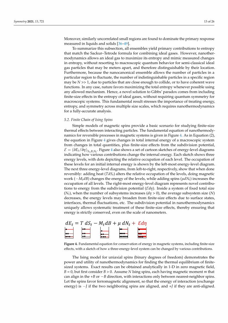
Simple models of magnetic spins provide a basic scenario for studying finite-sizethermal effects between interacting particles. The fundamental equation of nanothermody-namics for reversible processes in magnetic systems is given in Figure 4. As in Equation (2),the equation in Figure 4 gives changes in total internal energy of a macroscopic systemfrom changes in total quantities, plus finite-size effects from the subdivision potential,E = (∂Et/∂η)St ,B,Nt

. Figure 4 also shows a set of cartoon sketches of energy-level diagramsindicating how various contributions change the internal energy. Each sketch shows threeenergy levels, with dots depicting the relative occupation of each level. The occupation ofthese levels for an initial internal energy is shown by the left-most energy-level diagram.The next three energy-level diagrams, from left-to-right, respectively, show that when donereversibly: adding heat (TdSt) alters the relative occupation of the levels, doing magneticwork (−MtdB) changes the energy of the levels, while adding spins (µdNt) increases theoccupation of all levels. The right-most energy-level diagram represents novel contribu-tions to energy from the subdivision potential (Edη). Inside a system of fixed total size(Nt), when the number of subsystems increases (dη > 0), the average subsystem size (N)decreases, the energy levels may broaden from finite-size effects due to surface states,interfaces, thermal fluctuations, etc. The subdivision potential in nanothermodynamicsuniquely allows systematic treatment of these finite-size effects, thereby ensuring thatenergy is strictly conserved, even on the scale of nanometers.

Symmetry 2021, 13, x FOR PEER REVIEW 13 of 25

finite-size effects in the entropy of ideal gases, without requiring quantum symmetry for macroscopic systems. This fundamental result stresses the importance of treating energy, entropy, and symmetry across multiple size scales, which requires nanothermodynamics for a fully-accurate analysis.

5.2. Finite Chain of Ising Spins Simple models of magnetic spins provide a basic scenario for studying finite-size

thermal effects between interacting particles. The fundamental equation of nanothermo-dynamics for reversible processes in magnetic systems is given in Figure 4. As in Equation (2), the equation in Figure 4 gives changes in total internal energy of a macroscopic system from changes in total quantities, plus finite-size effects from the subdivision potential, ℰ = (휕퐸 /휕휂) , , . Figure 4 also shows a set of cartoon sketches of energy-level diagrams indicating how various contributions change the internal energy. Each sketch shows three energy levels, with dots depicting the relative occupation of each level. The occupation of these levels for an initial internal energy is shown by the left-most energy-level diagram. The next three energy-level diagrams, from left-to-right, respectively, show that when done reversibly: adding heat (푇푑푆 ) alters the relative occupation of the levels, doing mag-netic work (−푀 푑퐵) changes the energy of the levels, while adding spins (휇푑푁 ) increases the occupation of all levels. The right-most energy-level diagram represents novel contri-butions to energy from the subdivision potential (ℰdη). Inside a system of fixed total size (Nt), when the number of subsystems increases (dη > 0), the average subsystem size (N) decreases, the energy levels may broaden from finite-size effects due to surface states, in-terfaces, thermal fluctuations, etc. The subdivision potential in nanothermodynamics uniquely allows systematic treatment of these finite-size effects, thereby ensuring that en-ergy is strictly conserved, even on the scale of nanometers.

Figure 4. Fundamental equation for conservation of energy in magnetic systems, including finite-size effects, with a sketch of how a three-energy-level system can be changed by various contribu-tions.

The Ising model for uniaxial spins (binary degrees of freedom) demonstrates the power and utility of nanothermodynamics for finding the thermal equilibrium of finite-sized systems. Exact results can be obtained analytically in 1-D in zero magnetic field, B = 0, but first consider B > 0. Assume N Ising spins, each having magnetic moment 퓂 that can align in the +B or −B direction, with interactions only between nearest-neighbor spins. Let the spins favor ferromagnetic alignment, so that the energy of interaction (exchange energy) is −J if the two neighboring spins are aligned, and +J if they are anti-aligned. The usual solution to the 1-D Ising model includes contributions to energy from 퓂B and from the exchange interaction, yielding the partition function [2,3]

푄 , , ≈ 푒 / cosh(퓂퐵/푘푇) + [푒 / + 푒 / sinh (퓂퐵) ] / . (12)

If B = 0, the resulting free energy becomes

퐴 = −푘푇 ln 푄 , ≈ −푁푘푇 ln[2cosh(퐽/푘푇)] (13)

The approximations in Equations (12) and (13) come from assuming large systems with negligible end effects, or equivalently spins in a ring. However, most real spin sys-tems do not form rings, so that these equations are valid only in the limit of large systems, 푁 → ∞. We now address finite-size effects explicitly.

Consider a finite linear chain of N + 1 spins, yielding a total of N interactions (“bonds”) between nearest-neighbor spins [70]. It is convenient to write the energy in

Figure 4. Fundamental equation for conservation of energy in magnetic systems, including finite-sizeeffects, with a sketch of how a three-energy-level system can be changed by various contributions.

The Ising model for uniaxial spins (binary degrees of freedom) demonstrates thepower and utility of nanothermodynamics for finding the thermal equilibrium of finite-sized systems. Exact results can be obtained analytically in 1-D in zero magnetic field,B = 0, but first consider B > 0. Assume N Ising spins, each having magnetic moment m thatcan align in the +B or −B direction, with interactions only between nearest-neighbor spins.Let the spins favor ferromagnetic alignment, so that the energy of interaction (exchangeenergy) is −J if the two neighboring spins are aligned, and +J if they are anti-aligned.

Symmetry 2021, 13, 721 14 of 26

The usual solution to the 1-D Ising model includes contributions to energy from mB andfrom the exchange interaction, yielding the partition function [2,3]

QN,B,T ≈

eJ/kT cosh(mB/kT) +[e−2J/kT + e2J/kTsin h2(mB)

]1/2N

. (12)

If B = 0, the resulting free energy becomes

A = −kT ln QN,T ≈ −NkT ln[2cos h(J/kT)] (13)

The approximations in Equations (12) and (13) come from assuming large systemswith negligible end effects, or equivalently spins in a ring. However, most real spin systemsdo not form rings, so that these equations are valid only in the limit of large systems,N → ∞ . We now address finite-size effects explicitly.

Consider a finite linear chain of N + 1 spins, yielding a total of N interactions (“bonds”)between nearest-neighbor spins [70]. It is convenient to write the energy in terms of thebinary states of each bond, bi = ±1. Using +J for the energy of anti-aligned neighboringspins, and −J between aligned neighbors. The Hamiltonian is

E = −J ∑Ni=1 bi, with bi = −1,+1. (14)

Assuming x high-energy bonds (bi = −1), with (N − x) low-energy bonds (bi = +1),the internal energy is E = −J(N − 2x). The multiplicity of ways for this energy to occur isgiven by the binomial coefficient

Ω =2N!

x!(N − x)!= 2

(Nx

). (15)

The factor of 2 in Equation (15) is needed to accommodate both alignments of neigh-boring spins for each type of bond. The thermal properties of this finite-chain Ising modelin various ensembles are given in Table 2. Note that although the summation for thenanocanonical ensemble starts at N = 0, because the number of spins is N + 1 everyregion contains at least one spin, as required for spontaneous changes in the number ofsubsystems [57]. Additionally, note that due to end effects, the Helmholtz free energyfrom Table 2 for N − 1 bonds (N spins) is A = −(N − 1)kT ln[2 cosh(J/kT)] − ln 2, ap-proaching Equation (13) only when N → ∞ . Thus, if an unbroken chain is forced to have amacroscopic number of spins, all ensembles yield similar results. However, if the lengthof the chain can change by adding or removing spins at either end, thermal equilibriumrequires the nanocanonical ensemble. As with the ideal gas, this nanocanonical ensembleis the only ensemble that does not externally constrain the sizes of the regions, so thatthe system itself can find its equilibrium average and distribution of sizes. From Table 2,setting the subdivision potential to zero yields an average number of spins in each chain of:N + 1 = cosh(J/kT) + 1. Thus, at high temperatures the average chain contains two spinsconnected by one bond, whereas when T → 0 the average chain length diverges.

Symmetry 2021, 13, 721 15 of 26

Table 2. N + 1 Ising spins (N bonds) in zero field with x high-energy bonds (+J) and (N − x) low-energy bonds (−J).

Ensemble Partition Function Fundamental Thermodynamic Function and Variables

Microcanonical(N + 1,x) Ω = 2N!

x! (N−x)!Smc/k = ln(Ω) = ln[N!] + ln(2)− ln[x!]− ln[(N − x)!]≈ N ln(N)− x ln(x)− (N − x) ln(N − x)− ln[

√2πx(1− x/N)]

canonical(N + 1,T) Q =

N∑

x=0Ω e

(N−2x)JkT

A/kT = − ln(Q) = − ln[2(eJ/kT + e−J/kT)N

]= −N ln[2 cosh(J/kT)]− ln(2)E/J = (2x− N) = −Ntan h(J/kT)µ/kT = − ln[2cos h(J/kT)]Sc/k =

(E− A

)/kT = −N(J/kT) tan h(J/kT)+ N ln[2 cosh(J/kT)]+ ln(2)

Nanocanonical(µ,T) Y =

∞∑

N=0Q e

(N+1)µkT

Enc/kT = − ln(Y)= ln

[12 e−µ/kT − cosh(J/kT)

]= 0→ µ/kT = − ln2[cosh(J/kT) + 1]

N + 1 = ∂ ln(Y)/∂(µ/kT)= 1

2 e−µ/kT = cosh(J/kT) + 1→ µ/kT = − ln

2[N + 1

]Snc/k =

(E− µN − Enc

)/kT =

−N(J/kT) tan h(J/kT) + N ln2[cosh(J/kT) + 1]

As expected, Table 2 shows that the entropy of Ising spins increases with decreasing con-straints, so that again (as in Table 1) the nanocanonical ensemble has the highest total entropy.Specifically, the entropy per bond in the nanocanonical ensemble exceeds that in the canonicalensemble by the difference ∆S/Nk = (Snc − Sc)/Nk = ln[cosh(J/kT) + 1]/ cosh(J/kT)− ln(2)/N = ln

[(N + 1

)/N]− ln(2)/N. At high T where N → 1 , ∆S/Nk→ 0 . At low

T where N 1, ∆S/Nk ≈ 1/N − ln(2)/N → 0 . Numerical solution yields a maximumentropy difference of nearly 6% (∆S/Nk = 0.0596601 . . . ) at kT/J = 0.687297 . . . where N =2.25889 . . . Hence, Ising spins in the nanocanonical ensemble always have higher entropythan if they were constrained to be in the canonical ensemble, but the excess is small at bothlow, and high T. Nevertheless, if a mechanism exists to change the length of the system,an infinite chain will shrink until there is on average N + 1 = cosh(J/kT) + 1 spins in eachregion, thereby maximizing the entropy of system plus its environment with no externalconstraints on the internal heterogeneity. In fact, because it can be difficult to fix the size ofinternal regions, their size should vary without external constraints, limiting the usefulnessof the canonical ensemble for describing finite-size effects inside most real systems.

A key feature of the nanocanonical ensemble is that thermal equilibrium is found bysetting the subdivision potential to zero [57]. Indeed, Enc = 0 ensures that the system findsits own equilibrium distribution of regions, without external constraint, similar to howµ = 0 in standard statistical mechanics yields the equilibrium distribution of phonons andphotons, without external constraint. Specifically, because Enc is the change in the totalenergy with respect to the number of subsystems, spontaneous changes in η occur unlessEnc = 0. However, Enc = −kT ln(Y) = 0 requires Y = 1 without any normalization, so thatall factors must be carefully included in the partition function. For example, supposethat the factor of 2 in the numerator of Ω (Equation (15)) is ignored from neglecting thedegeneracy of each sequence of spins and its inversion. Because averages in the canonicalensemble (e.g., E) are normalized by the partition function, they do not change, but theaverage number of bonds in the nanocanonical ensemble becomes N = 2 cosh(J/kT), twicethe value of N = cosh(J/kT) from Table 2.

5.3. The Subdivided Ising Model: Ising-Like Spins with a Distribution of Neutral Bonds

Results similar to those for the finite-size Ising model in the nanocanonical ensemble(Section 5.2) can be obtained in the canonical ensemble by modifying the Ising model toinclude “neutral bonds,” from nearest-neighbor spins that do not interact. (Our modeldiffers from dilute Ising models [71] that assume empty lattice sites at fixed locations.)Physically, neutral bonds may come from neighboring spins having negligible quantumexchange (which suppresses their interaction), or from neighboring spins with uncorrelatedfluctuations so that their interaction is time averaged to zero. Again, start with the standard

Symmetry 2021, 13, 721 16 of 26

Ising model having N + 1 spins (N bonds), but now let there be η’ neutral bonds (yieldingη = η’ + 1 subsystems). In addition, let there be x high-energy bonds between anti-alignedspins, leaving N − η’ + 1 − x low-energy bonds between aligned spins. Figure 5 shows aspecific configuration of 11 spins (N = 10 bonds) with x = 2 high-energy bonds (X), η’ = 3neutral bonds (O), and N − η’ − x = 5 low-energy bonds (•). It is again convenient to writethe energy in terms of the bonds, which may now have three distinct states, yielding theHamiltonian

E = −J ∑Ni=1 bi, with bi = −1, 0,+1. (16)

Symmetry 2021, 13, x FOR PEER REVIEW 15 of 25

external constraints on the internal heterogeneity. In fact, because it can be difficult to fix the size of internal regions, their size should vary without external constraints, limiting the usefulness of the canonical ensemble for describing finite-size effects inside most real systems.

A key feature of the nanocanonical ensemble is that thermal equilibrium is found by setting the subdivision potential to zero [57]. Indeed, ℰ = 0 ensures that the system finds its own equilibrium distribution of regions, without external constraint, similar to how μ = 0 in standard statistical mechanics yields the equilibrium distribution of phonons and photons, without external constraint. Specifically, because ℰ is the change in the total energy with respect to the number of subsystems, spontaneous changes in η occur unless ℰ = 0. However, ℰ = −푘푇 ln(Υ) = 0 requires Υ = 1 without any normaliza-tion, so that all factors must be carefully included in the partition function. For example, suppose that the factor of 2 in the numerator of Ω (Equation 15) is ignored from neglecting the degeneracy of each sequence of spins and its inversion. Because averages in the ca-nonical ensemble (e.g., 퐸) are normalized by the partition function, they do not change, but the average number of bonds in the nanocanonical ensemble becomes 푁 =2 cosh(퐽/푘푇), twice the value of 푁 = cosh(퐽/푘푇) from Table 2.

5.3. The Subdivided Ising Model: Ising-Like Spins with a Distribution of Neutral Bonds Results similar to those for the finite-size Ising model in the nanocanonical ensemble

(Section 5.2) can be obtained in the canonical ensemble by modifying the Ising model to include “neutral bonds,” from nearest-neighbor spins that do not interact. (Our model differs from dilute Ising models [71] that assume empty lattice sites at fixed locations.) Physically, neutral bonds may come from neighboring spins having negligible quantum exchange (which suppresses their interaction), or from neighboring spins with uncorre-lated fluctuations so that their interaction is time averaged to zero. Again, start with the standard Ising model having 푁 + 1 spins (N bonds), but now let there be η’ neutral bonds (yielding η = η’ + 1 subsystems). In addition, let there be x high-energy bonds between anti-aligned spins, leaving N − η’ + 1 − x low-energy bonds between aligned spins. Figure 5 shows a specific configuration of 11 spins (N = 10 bonds) with x = 2 high-energy bonds (X), η’=3 neutral bonds (O), and N − η’ − x = 5 low-energy bonds (). It is again convenient to write the energy in terms of the bonds, which may now have three distinct states, yield-ing the Hamiltonian

퐸 = −퐽 ∑ 푏 , with bi = –1,0,+1. (16)

The internal energy of the system is 퐸 = −퐽(푁 − 휂′ − 2푥). The canonical ensemble involves two sums. The first sum is over x for fixed η’, with a multiplicity given by the trinomial coefficient for the number of ways that the high- and low-energy bonds can be arranged among N − η’ interacting bonds. An extra factor of 2η’ arises because each neutral bond has two possible states for its neighboring spin. This first sum yields a type of ca-nonical ensemble for the system with fixed η’. A second sum is over all values of η’. The multiplicity is given by the binomial for the number of ways that the neutral bonds can be distributed, which arises from the trinomial after the first summation. The behavior of this model is summarized in Table 3.

Figure 5. Sketch of 11 Ising-like spins in a chain connected by N = 10 bonds. Here, η’ = 3 bonds are neutral (O) (yielding η = 4 regions), x = 2 bonds are high-energy (X), and N − η’ − x = 5 bonds are low energy ().

Figure 5. Sketch of 11 Ising-like spins in a chain connected by N = 10 bonds. Here, η’ = 3 bonds areneutral (O) (yielding η = 4 regions), x = 2 bonds are high-energy (X), and N − η’ − x = 5 bonds arelow energy (•).

The internal energy of the system is E = −J(N − η′ − 2x). The canonical ensembleinvolves two sums. The first sum is over x for fixed η’, with a multiplicity given by thetrinomial coefficient for the number of ways that the high- and low-energy bonds canbe arranged among N − η’ interacting bonds. An extra factor of 2η’ arises because eachneutral bond has two possible states for its neighboring spin. This first sum yields a typeof canonical ensemble for the system with fixed η’. A second sum is over all values of η’.The multiplicity is given by the binomial for the number of ways that the neutral bondscan be distributed, which arises from the trinomial after the first summation. The behaviorof this model is summarized in Table 3.

Table 3. N + 1 Ising-like spins with η’ neutral bonds (energy = 0), x high-energy bonds (+J), and N − η’ − x low-energybonds (−J).

Ensemble Partition Function Fundamental Thermodynamic Function and Variables

microcanonical(N + 1,η’,x) Ω = 2N! 2η′

x!η′!(N−η′−x)!Smc/k = ln(Ω) = ln[N!] + ln

(2η′+1)− ln[x!]− ln[η′!]− ln[(N − η′ − x)!]

≈ N ln(N)− x ln(x)− η′ ln(η′/2)− (N − η′ − x) ln(N − η′ − x)

quasi-canonical(N + 1,η’,T) Z =

N−η′∑

x=0Ω e

(N−η′−2x)JkT

Z = 2N+1[cosh( J

kT

)]N−η′N!/[η′!(N − η′)!]

N − η′ − 2x = ∂ ln Z/∂(J/kT) = (N − η′)tanh(J/kT)E/J = −(N − η′ − 2x) = −(N − η′)tan h (J/kT)

canonical(N + 1,T) Q =

N∑

η′=0

N!η′!(N−η′)! Z

A/kT = − ln(Q) = −(N + 1) ln(2)− N ln[1 + cos h(J/kT)]N − η′ = cosh(J/kT)∂ ln Q/∂cos h(J/kT) =N cosh(J/kT)]/[1 + cosh(J/kT)]E/J = −(N − η′)tan h (J/kT) = −Nsinh(J/kT)/[1 + cosh(J/kT)]Sc/k = −N(J/kT)sinh(J/kT)/[1 + cosh(J/kT)] + N ln[1 + cosh(J/kT)]

We now compare the results in Table 3 for the subdivided Ising model with those fromTable 2 for the finite-size Ising model. In the canonical ensemble, the average energy ofthe subdivided system is higher (not as negative) as that of the finite system, as expectedwhen neutral bonds replace an equilibrium mixture of predominantly low-energy bonds.However, the average energy per interacting bond (E from Table 3, divided by N − η′) is−Jtanh(J/kT), the same as E/N from Table 2. Another similarity comes from using theaverage number of subsystems, η′ = N/[1 + cosh(J/kT)], to obtain the average numberof spins in each region,

n =N + 1η′+ 1

=1 + cosh(J/kT)

1 + [cosh(J/kT)]/(N + 1)(17)

Symmetry 2021, 13, 721 17 of 26

Hence, in the limit of N → ∞ , Equation (17) gives n− 1 ≈ cosh(J/kT) for the averagenumber of bonds in the subdivided Ising model in the canonical ensemble, approachingN = cosh(J/kT) from Table 2 for the finite-size Ising model in the nanocanonical ensemble.In other words, if the initial system is large enough, both approaches to nanothermody-namics are equivalent: a large ensemble of small systems (Table 2) and a large system thatis repeatedly subdivided into independent subsystems (Table 3). Furthermore, modelswith distinct Hamiltonians—Equation (16) here for a system of three-state bonds andEquation (14) for a system of two-state bonds—may yield equivalent results. However,equivalence requires that the correct ensemble is used for each system, canonical ensemblehere for the subdivided Ising model, and nanocanonical in Section 5.2. Thus, the choiceof ensemble is crucial for obtaining fully-accurate behavior, even for systems that are inthermal equilibrium and in the thermodynamic limit.

5.4. Finite Chains of Effectively Indistinguishable Ising-Like Spins

We now consider an Ising-like model with local symmetry from particle exchangethat allows nanoscale regions in the system to mimic the statistics of indistinguishableparticles. Although the standard Ising model assumes that each spin can be distinguishedby its location, the main mechanism causing ferromagnetism is the exchange interactionthat occurs only between indistinguishable particles. Finite-size effects on the scale ofnanometers inside bulk samples can be attributed to symmetry from particle exchangethat is spatially localized within regions, causing the heterogeneity that defines the re-gions. Another consequence of particle exchange is that interaction energies are not static,i.e., the alignment between neighboring spins is not fixed, which decreases the multiplic-ity of degenerate energy states that become indistinguishable. Here, we discuss someconsequences of nanoscale symmetry on simple systems.

We again start with the finite-size Ising model comprised of a linear chain of N bondsbetween N + 1 spins. The Hamiltonian (Equation (14)) yields the interaction energy E =−J(N − 2x) for x high-energy bonds and (N − x) low-energy bonds. The average energy inthe canonical ensemble is given by

E = −J ∑Nx=0 Ω(N − 2x)e(N−2x)J/kT

∑Nx=0 Ωe(N−2x)J/kT

Ω =

2(

Nx

)distinguishable

2 indistinguishable

(18a)(18b)

The binomial coefficient for the multiplicity of distinguishable states, Equation (18a),yields the usual expression for the average energy of the Ising model, E = −NJtanh(J/kT),as given in Table 2. However, if excited states are distinguishable by their macrostate(number of high-energy bonds x), but not by their microstate (location of each bond),then most states have their degeneracy reduced. We assume that all energy states aredoubly degenerate, Equation (18b), attributable to the Pauli exclusion principle for spin- 1

2particles, yielding results that are summarized in Table 4. Note that the average energymimics the Brillouin function, consistent with regions having degenerate discrete states.

Table 4. N + 1 Ising-like spins, N indistinguishable bonds: x high-energy bonds (+J) and (N − x) low-energy bonds (−J).

Ensemble Partition Function Fundamental Thermodynamic Function and Variables

microcanonical(N,x) Ω = 2 Smc/k = ln(Ω) = ln(2)

canonical(N,T) Q =

N∑

x=0Ω e

(N−2x)JkT

A/kT = − ln(Q) = − ln2sinh[(N + 1)J/kT]/sinh(J/kT)E/J = (2x− N) = −(N + 1)cot h[(N + 1)J/kT]+coth(J/kT)µ/kT = ln[sinh(NJ/kT)]− lnsin h[(N + 1)J/kT]Sc/k =

(E− A

)/kT

nanocanonical(µ,T) Y =

∞∑

N=0Q e

(N+1)µkT

Enc/kT = − ln(Y) = ln[cosh(µ/kT)− cosh(J/kT)]= 0µ/kT = −acosh[cosh(J/kT) + 1]

N + 1 =√[cosh(J/kT) + 1]2 − 1

Snc/k =(E− µN − Enc

)/kT

Symmetry 2021, 13, 721 18 of 26

5.5. Entropy and Heat in an Ideal 1-D Polymer

Although adiabatic demagnetization provides a well-known connection between en-tropy and heat in spin systems [4,41,72], this connection is often more familiar in the contextof ideal polymers. Furthermore, the basic behavior of the polymer can be experienced athome using a rubber band [73]. Here, for a simplified analysis related to the 1-D Isingmodel, we treat an ideal polymer comprised of freely jointed monomers (units) in 1-D [6].Consider a polymer of N units, each of length a. Let one end of the 1st unit be freelyjointed (free to invert) about the origin (X = 0), with the far end of the Nth unit unconnected.All other units have both ends freely jointed to neighboring units. For simplicity assume allunits are uniaxial (1-D), with x segments pointing in the –X direction and N − x segmentsin the +X direction. The free end of the polymer is at position X(x) = (N − 2x) a. The multi-plicity matches that of Equation (18a) for the standard Ising model, and Table 2 gives the

resulting microcanonical entropy Smc/k = ln[

2(

Nx

)]. The elastic restoring force from

the entropy [1] is: F = − T ∆S/∆X Note that this model involves differences (not differen-tials) because it is comprised of discrete polymer units in 1-D. Such discrete differencescircumvent Stirling’s formula, improving the accuracy, especially for small systems. For anincremental shortening of the polymer ∆X = −2a, using half integers to best representthe average values at each integer, the change in configurational entropy of the polymer

is ∆Smc/k = ln[

N!(x+ 1

2 )!(N−x− 12 )!

]− ln

[N!

(x− 12 )!(N−x+ 1

2 )!

]= ln

[N−x+ 1

2x+ 1

2

]. Solving for the

average number of negatively aligned units as a function of F gives x =N+ 1

2 (1−e2aF/kT)1+e2aF/kT ,

yielding the equilibrium endpoint of the polymer X(x) = (N + 1) atanh(aF/kT). At high-temperatures X(x) ≈ (N + 1) a2F

kT , similar to the standard expression for the ideal 1-Dpolymer if N >> 1.

This model shows a common characteristic of polymers under tension: their averagelength varies inversely proportional to temperature. This decrease in X with increasing T,opposite to the behavior of most other solids, arises from the dominance of configurationalentropy in polymers. Such length contraction can be observed by heating a rubber bandthat holds a hanging mass, demonstrating a simple conversion of heat into work. The con-verse conversion of work into heat can be experienced by the increased temperature of arubber band that is rapidly stretched while in contact with your lips. Cyclic heat-to-workconversion is shown by the heat engine made from a wheel with rubber-band spokes,where an incandescent lamp causes the wheel to rotate continuously [73]. The heat-to-workmechanism comes from increased thermal agitation around the polymer, increasing itsentropy and coiling it more tightly. Similarly, the work-to-heat conversion involves energyadded to the heat bath when entropy is reduced as the polymer is stretched.

The purpose of this brief digression is to emphasize how changing the configurationalentropy of a polymer by changing its length alters the energy of the heat bath, thus alteringthe entropy of the bath. We assume that an analogous change in the entropy of the polymerduring a fluctuation causes a similar exchange of entropy with the bath. In other words, weassume that the heat bath cannot discern whether changes in entropy of a polymer are dueto external forces, or internal fluctuations. Next, we assume that equilibrium (reversible)fluctuations occur with no net loss in entropy, so that the second law of thermodynamics isstrictly obeyed. Specifically, we make the ansatz that during equilibrium fluctuations theentropy of the polymer plus the entropy of its local heat bath (SL(X)) never deviate from amaximum value:

S(X) + SL(X) = Smax (19)

We now expand on the concept of local heat baths in nanothermodynamics [35,74] toshow how Equation (19) facilitates reversible fluctuations. In standard thermodynamics,reversible processes must proceed at infinitesimal rates, allowing the system to coupleuniformly to the effectively infinite heat reservoir. However, many thermal fluctuationsare fast and heterogeneous. Nanothermodynamics is based on independent small systems,

Symmetry 2021, 13, 721 19 of 26

often with energy and entropy isolated from neighboring systems, consistent with theenergy localization and local T deduced from experiments [36–42] and simulations [50].For the specific model presented here, imagine a large sample containing a polymermelt. Let independent polymers (or their independent monomers [49,58]) and a localheat bath occupy a nanoscale volume inside the sample. During fast fluctuations, eachvolume is effectively isolated from neighboring volumes, conserving local energy and localentropy (Equation (19)), characteristic of the microcanonical ensemble (upper-left boxesin Figure 1). Note, however, that for fluctuations about equilibrium, the microcanonicalboxes would have a distribution of sizes and shapes, basically a frozen snapshot of thelower-right regions in Figure 1. During sufficiently slow fluctuations, energy and particlescan transfer freely between variable volumes to maximize the total entropy and maintain athermal equilibrium distribution of regions in the nanocanonical ensemble. Thus, accurateevaluation of thermal fluctuations often involves two ensembles, the fully-closed ensemblefor fast fluctuations, and the fully-open ensemble for slow fluctuations. Partially-openensembles (e.g., canonical and grand-canonical), which restrict the exchange of somequantities but not others, are often artificially constrained. Specifically, because excessenergy is persistently localized during the primary response in liquids, glasses, polymers,and crystals [36–42], sometimes for seconds or longer, particle exchange will usuallyaccompany these slow changes in energy. Therefore, the relatively fast transfer of energyneeded for a well-defined local temperature, without also changing size and particlenumber, is unlikely for the primary fluctuations inside most realistic systems.

We now evaluate equilibrium fluctuations that include energy from configurationalentropy, which is often ignored in standard fluctuation theory. Let there be no external forceon the polymer, so that the average position of its endpoint is X(x) = 0, corresponding toits maximum configurational entropy. From Equation (19), as S(X) decreases when X 6= 0,SL(X) must increase, and vice versa. Quantitatively, using the microcanonical entropyfor the polymer (adapted from Table 2), allowing fast fluctuations that are localized andreversible, the entropy of the local bath is:

SL(X) = Smax − ln(N!) + ln[(N − X)/2]!+ ln[(N + X)/2]! (20)

We assume that Boltzmann’s factor, commonly used to weight large-reservoir states,also weights the local-bath states wL = eSL(X)/k. Thus, when thermally averaged, everylength of the polymer is equally likely, wL Ω = eSL(X)/keS(X)/k = eSmax/k. In other words,maintaining maximum entropy during equilibrium fluctuations removes degeneraciesfrom systems of classical particles that have the same macrostate (e.g., same X, N, or E),mimicking the statistics of indistinguishable particles. In previous work it has been shownthat removing the alignment degeneracy from systems with the same X yields 1/f -likenoise, with several features that match the low-frequency fluctuations measured in metalfilms and tunnel junctions [17,74–76]. Here, we describe how removing the energy de-generacy from systems with the same E yields similar 1/f -like noise at lower frequencies,combined with Johnson-Nyquist-like (white) noise at higher frequencies.

5.6. Simulations of Finite Chains of Effectively Indistinguishable Ising-Like Spins

We explore consequences of including contributions from configurational entropy inthe total energy during equilibrium fluctuations. The manner in which we add this entropyreduces the degeneracy of most energy states, mimicking the statistics of indistinguishableparticles, Equation (18b). We study the 1-D Ising model using Monte Carlo (MC) simula-tions for the dynamics. The 1-D Ising model is used for simplicity, having its multiplicityof energy states given exactly by the binomial coefficient in Equation (18a). Although MCsimulations are too simplistic for microscopic dynamics, they can accurately simulate slowthermal processes around equilibrium [77,78]. A novel ingredient in our simulations isto introduce a type of orthogonal dynamics, where changes in energy are independent ofchanges in alignment. Specifically, each MC step conserves energy, or alignment, with nostep allowing both to change simultaneously. Such constraints on the dynamics can be jus-

Symmetry 2021, 13, 721 20 of 26

tified by the fact that energy and alignment contribute to distinct thermodynamic variables,and each is governed by a separate conservation law. Analogous decoupling of degrees offreedom has been found in supercooled fluids [79,80]. This orthogonal Ising model yieldsa combination of 1/f -like noise at low frequencies, and white noise at higher frequencies,similar to behavior often found in nature.

We start with a finite chain of Ising spins (Section 5.2), with ferromagnetic interactionJ between nearest-neighbor spins. The Hamiltonian is given by Equation (14). Considera state containing x high-energy bonds and N − x low-energy bonds. The interactionenergy of this state is E = −J(N − 2x), and its multiplicity is the binomial coefficient

Ω = 2(

Nx

). Equilibrium behavior of this model in various thermodynamic ensembles

is given in Table 2, but these results restrict Boltzmann’s factor to include only the internalenergy from interactions. We now explore how adding the energy from configurationalentropy alters the behavior.

The Metropolis algorithm is often used to efficiently yield the Boltzmann distributionof energy states in MC simulations. A standard MC simulation of the Ising model involveschoosing a spin at random, then inverting the spin if its change in interaction energy (∆E)meets the Metropolis criterion

e−∆E/kT > [0, 1) (21)

where [0,1) is a random number uniformly distributed between 0 and 1. This criterioncomes from energy transfer with an ideal (effectively infinite and homogeneous) heatreservoir due to changes in interaction energy; but crucial sources of energy from config-urational entropy and the local thermal bath are neglected. We therefore add a secondcriterion that must also be met if configuration changes

e−∆S(X)/k > [0, 1) (22)

where ∆S(X) = SL(X). Note that Equation (22) favors high entropy in the local bath, just asEquation (21) favors high energy (and hence high entropy) in a large reservoir. Additionally,note that Equation (19) gives SL(X) = Smax − S(X), the offset between the maximumconfigurational entropy and its current value, not just the change in entropy between initialand final states. Justification comes from the assumption that fast fluctuations involve localproperties that do not have time to couple to the large reservoir, and even localized thermalprocess must not diminish the total entropy. Furthermore, S(X) for finite systems involvesnonlinear terms that cannot be reduced to linear differentials.

Symbols in Figure 6 show histograms of the energy from the Ising model at fourtemperatures, using the standard Metropolis algorithm (open), and when contributionsfrom configurational entropy are added (solid). Solid curves come from the integrand inthe numerator of Equation (18a), showing that using Equation (21) alone yields the statisticsof distinguishable states, whereas dashed lines come from the integrand in the numeratorof Equation (18b), showing that adding Equation (22) yields behavior characteristic of thestatistics of indistinguishable states.

We now describe a dynamical sequence for simulating the Ising model which separatesenergy-changing steps from alignment-changing steps, thereby separating the fundamentallaws of conservation of energy and conservation of angular momentum. For this orthogonalIsing model, alignment is conserved using Kawasaki dynamics [81], where neighboringspins exchange their alignments, or equivalently they exchange their locations withoutchanging their alignments. This exchange always conserves the net alignment, but netenergy often changes. Alternatively, alignment is changed without changing energy byinverting only spins that have oppositely oriented neighbors. The simulation proceeds byfirst choosing a spin at random from the chain, then randomly choosing whether to attempta spin exchange or a spin flip. If spin flip is chosen, and only if the spin’s neighbors areoppositely aligned, then the spin is inverted, changing the net alignment without changingthe interaction energy. If instead spin exchange is chosen, and if the configurational-entropy

Symmetry 2021, 13, 721 21 of 26

criterion is met (Equation (22)), then one of its nearest-neighbor spins is chosen at random.If exchanging the alignments of these two spins also meets the interaction-energy criterion(Equation (21)) then spin exchange occurs, always preserving net alignment, but oftenchanging the interaction energy.

Symmetry 2021, 13, x FOR PEER REVIEW 20 of 25

where [0,1) is a random number uniformly distributed between 0 and 1. This criterion comes from energy transfer with an ideal (effectively infinite and homogeneous) heat res-ervoir due to changes in interaction energy; but crucial sources of energy from configura-tional entropy and the local thermal bath are neglected. We therefore add a second crite-rion that must also be met if configuration changes

푒 ( )/ > [0,1) (22)

where ΔS(X) = SL(X). Note that Equation (22) favors high entropy in the local bath, just as Equation (21) favors high energy (and hence high entropy) in a large reservoir. Addition-ally, note that Equation (19) gives SL(X) = Smax − S(X), the offset between the maximum configurational entropy and its current value, not just the change in entropy between ini-tial and final states. Justification comes from the assumption that fast fluctuations involve local properties that do not have time to couple to the large reservoir, and even localized thermal process must not diminish the total entropy. Furthermore, S(X) for finite systems involves nonlinear terms that cannot be reduced to linear differentials.

Symbols in Figure 6 show histograms of the energy from the Ising model at four tem-peratures, using the standard Metropolis algorithm (open), and when contributions from configurational entropy are added (solid). Solid curves come from the integrand in the numerator of Equation (18a), showing that using Equation (21) alone yields the statistics of distinguishable states, whereas dashed lines come from the integrand in the numerator of Equation (18b), showing that adding Equation (22) yields behavior characteristic of the statistics of indistinguishable states.

Figure 6. Internal energy distributions from a 1-D Ising model with N = 50 bonds at four temperatures, given in the legend. Symbols show histograms from simulations using the usual Metropolis algorithm that includes only interaction energy (open), and when an offset entropy term is added (solid). Lines are fits to the data using the integrand in the numerator of Equation (18a) (solid) or Equation (18b) (dashed).

-0.8 -0.4 0.0 0.4 0.8

1

10

100

1,000

10,000

Freq

uenc

y (c

ount

s)

E/NJ

kT/J = 2 5 10 1,000

Figure 6. Internal energy distributions from a 1-D Ising model with N = 50 bonds at four temperatures, given in the legend.Symbols show histograms from simulations using the usual Metropolis algorithm that includes only interaction energy(open), and when an offset entropy term is added (solid). Lines are fits to the data using the integrand in the numerator ofEquation (18a) (solid) or Equation (18b) (dashed).

Solid lines in Figure 7 show frequency-dependent power spectral densities (S(f ))from simulations of the orthogonal Ising model (solid lines) and from measured fluxnoise in a qubit (symbols) [82]. Simulated S(f ) comes from the magnitude squared ofthe Fourier transform of time-dependent fluctuations in alignment. Note the generalfeature that large chains exhibit a low-frequency 1/f -like regime that crosses over to awhite noise regime at higher frequencies. Thus, this model has a single thermodynamicvariable that exhibits both types of thermal noise that are usually found together in nature.The basic mechanism involves slowly-fluctuating energy (with 1/f -like noise due to theentropy-change constraint), which slowly modulates an envelope that limits the maximumamplitude for the fast-fluctuating alignment. The orthogonal dynamics is crucial to preventall other intermixing between distinct thermodynamic variables.

Symmetry 2021, 13, 721 22 of 26

Symmetry 2021, 13, x FOR PEER REVIEW 21 of 25

We now describe a dynamical sequence for simulating the Ising model which sepa-rates energy-changing steps from alignment-changing steps, thereby separating the fun-damental laws of conservation of energy and conservation of angular momentum. For this orthogonal Ising model, alignment is conserved using Kawasaki dynamics [81], where neighboring spins exchange their alignments, or equivalently they exchange their loca-tions without changing their alignments. This exchange always conserves the net align-ment, but net energy often changes. Alternatively, alignment is changed without changing energy by inverting only spins that have oppositely oriented neighbors. The simulation proceeds by first choosing a spin at random from the chain, then randomly choosing whether to attempt a spin exchange or a spin flip. If spin flip is chosen, and only if the spin’s neighbors are oppositely aligned, then the spin is inverted, changing the net align-ment without changing the interaction energy. If instead spin exchange is chosen, and if the configurational-entropy criterion is met (Equation (22)), then one of its nearest-neigh-bor spins is chosen at random. If exchanging the alignments of these two spins also meets the interaction-energy criterion (Equation (21)) then spin exchange occurs, always pre-serving net alignment, but often changing the interaction energy.

Solid lines in Figure 7 show frequency-dependent power spectral densities (S(f)) from simulations of the orthogonal Ising model (solid lines) and from measured flux noise in a qubit (symbols) [82]. Simulated S(f) comes from the magnitude squared of the Fourier transform of time-dependent fluctuations in alignment. Note the general feature that large chains exhibit a low-frequency 1/f-like regime that crosses over to a white noise regime at higher frequencies. Thus, this model has a single thermodynamic variable that exhibits both types of thermal noise that are usually found together in nature. The basic mecha-nism involves slowly-fluctuating energy (with 1/f-like noise due to the entropy-change constraint), which slowly modulates an envelope that limits the maximum amplitude for the fast-fluctuating alignment. The orthogonal dynamics is crucial to prevent all other in-termixing between distinct thermodynamic variables.

100 1,000 10,000

7

8

9

2 4 6 8 10 12

-60

-40

-20

0 f

C = 1010.1/N 0.81

log(

f C /

f 0 )

System Size (N)

fc(1,000)

System Size N = 32 50 100 1,000 10,000

S( f ) ~ 1/f 0.92

Yan et al., Nat. comm. 4, 3337 (2013)

S( f

) (dB

) + 1

0 lo

g(N

)

log( f / f0 )

Figure 7. Frequency dependence of power spectral densities. Solid lines are from several simulations of an orthogonal Isingmodel about an average temperature of kT/J ~ 200, with system size (N) given in the legend. Solid circles show measuredflux noise from a qubit [82]. The characteristic frequency (f 0) and amplitude of the simulations have been offset so thatN = 50 (red line) mimics the data, with no other adjustable parameters. The dashed line fitted to the N = 1000 simulationhas a slope of 0.92 ± 0.02, consistent with measurements of flux noise in qubits [83]. White noise (dotted line) occurs abovethe crossover frequency, f > f c. The inset shows the N dependence of this f c.

Broken lines in Figure 7 show linear fits to the 1000-bond chain for the 1/f -like(dashed) and white (dotted) noise regimes. The intersection of these lines (marked byan arrow) yields the crossover frequency, fc(1000). The inset in Figure 7 shows the chain-size dependence of this fc. Three distinct features shown by the simulations in Figure 7mimic measured noise in quantum bits [82,83]: 1/f -like noise with a slope of magnitude0.92 ± 0.02; S(f ) in smaller chains with discrete Lorentzian spectra; and white noise athigher frequencies. Figure 7 also shows that there are two ways to reduce low-frequencynoise in the orthogonal Ising model. Specifically, at log(f/f 0) = 4 maximum noise occurswhen N ≈ 50. Noise decreases for larger N as fc shifts to lower frequencies, and decreasesfor smaller N as 1/f -like noise saturates at low frequencies in small systems, avoidingthe divergence as f → 0 [76]. Thus, Figure 7 shows that the orthogonal Ising modelhas fluctuations in alignment that yield measured frequency exponents for 1/f -like noise,a crossover to white noise at higher f, and discrete Lorentzian responses; three distinctfeatures that mimic measured spectra.

6. Conclusions

The theory of small-system thermodynamics is needed to ensure conservation ofenergy and maximum entropy in the thermal and dynamic properties of systems overmultiple scales, especially on the scale of nanometers. Here, we have emphasized thatthis “nanothermodynamics” is also crucial for obtaining the thermal equilibrium of largesystems that can subdivide into an ensemble of independently fluctuating subsystems

Symmetry 2021, 13, 721 23 of 26

that we call “regions.” These regions are fully open—able to freely exchange energy andparticles between neighboring regions without external constraints—a unique feature ofthe “nanocanonical” ensemble that is well defined only in nanothermodynamics. Severalresults are presented to highlight various aspects of nanothermodynamics.

One result (Section 5.1) is to show how a large system of semi-classical ideal gas“atoms” increases its net entropy by subdividing into an ensemble of small regions. Atomsin each region are indistinguishable due to their proximity, but distinguishable from atomsin neighboring regions due to their separate locations. Thus, the need for macroscopicquantum symmetry for non-interacting point-like particles that may be meters apart isavoided. Atoms become indistinguishable only if they occupy the same nanoscale region,where they are close enough to have coherent wavefunctions, consistent with the usualcriterion for the onset of quantum behavior. If two macroscopic ensembles of these regionsare combined, they mimic the usual entropy of mixing for semi-classical ideal gas particles,providing a novel solution to Gibbs’ paradox from finite-size effects in thermodynamics.Careful analysis reveals that the sub-additive entropy found only in the nanocanonicalensemble may be difficult to measure directly due to long-range correlations in real gases.Nevertheless, because the total entropy decreases when an ideal gas is subdivided intofixed volumes in the canonical ensemble, the fundamental property of quantum mechanicsrequiring sub-additive entropy [23,68] also favors variable volumes in the nanocanonicalensemble.

Other results presented here come from models based on Ising-like “spins,” which aresolved analytically in 1-D. One example (Section 5.2) is a chain of spins with variable length,in thermal contact with an ensemble of similar chains, which lowers its free energy byforming a nanocanonical ensemble comprised of chains with an equilibrium distributionof all possible lengths. The average length approaches two spins (one bond) at hightemperatures, diverging to large systems only as the temperature goes to zero. Equivalentbehavior (Section 5.3) is found in the canonical ensemble for a three-state model in a singlechain of effectively infinite length. Section 5.4 describes the thermal behavior of a 1-D Ising-like model comprised of spin states with constant multiplicity, attributable to the exchangeinteraction between particles that makes many states indistinguishable. Sections 5.5 and 5.6describe how similar results are obtained by including nanoscale contributions to energyfrom configurational entropy during equilibrium fluctuations. Computer simulations(Section 5.6) show that an Ising model with orthogonal dynamics (to separate changesin energy from changes in alignment) exhibits three types of thermal noise often foundin nature. Specifically, the simulations show 1/f -like noise at low frequencies, Johnson-Nyquist-like white noise at higher frequencies, with discrete Lorentzian modes visible forsufficiently small systems.

In summary, nanothermodynamics provides a systematic way to calculate contribu-tions to energy and entropy across multiple size scales. A general result is that the correctensemble is needed to describe the fluctuations, internal dynamics, and thermal equilibriumof macroscopic systems, regardless of system size. Furthermore, different Hamiltonians inspecific ensembles can yield equivalent behavior, emphasizing the importance of includingall contributions to thermal energy, not just those from microscopic interactions. Anotherresult is a novel solution to Gibbs’ paradox that has quantum symmetry of semi-classicalideal gas particles over length scales of nanometers, but not across macroscopic samples.Additional insight into the thermal behavior of other systems may come from similarlystrict adherence to the laws of thermodynamics across multiple length scales.

Author Contributions: Conceptualization, R.V.C.; methodology, R.V.C.; software, R.V.C. and M.R.C.;validation, R.V.C., V.M. and G.H.W.; writing—original draft preparation, R.V.C.; writing—reviewand editing, R.V.C., V.M. and G.H.W.; All authors have read and agreed to the published version ofthe manuscript.

Funding: This research received no external funding.

Institutional Review Board Statement: Not applicable.

Symmetry 2021, 13, 721 24 of 26

Informed Consent Statement: Not applicable.

Data Availability Statement: Data presented here are available from the corresponding author.

Acknowledgments: We have benefited from computer simulations done by Tyler Altamirano. We ac-knowledge support from Arizona State University Research Computing for use of their facilities.We thank Sumiyoshi Abe for his careful reading of the manuscript, and his insightful comments.

Conflicts of Interest: The authors declare no conflict of interest.

References and Notes1. Callen, H.B. Thermodynamics and an Introduction to Thermostatistics, 2nd ed.; John Wiley & Sons: Hoboken, NJ, USA, 1985.2. Hill, T.L. Introduction to Statistical Thermodynamics; Dover: Mineola, NY, USA, 1986.3. Pathria, R.K.; Beale, P. Statistical Mechanics, 3rd ed.; Elsevier: Oxford, UK, 1996.4. Baierlein, R. Thermal Physics; Cambridge University Press: Cambridge, UK, 1999.5. McQuarrie, D.A. Statistical Mechanics; University Science Books: Sausalito, CA, USA, 2000.6. Schroeder, D.V. An Introduction to Thermal Physics; Addison-Wesley: Boston, MA, USA, 2000.7. Ghosh, K.; Dill, K.A.; Inamdar, M.M.; Seitaridou, E.; Phillips, R. Teaching the principles of statistical dynamics. Am. J. Phys. 2006,

74, 123–133. [CrossRef]8. Jarzynski, C. Equalities and inequalities: Irreversibility and the second law of thermodynamics at the nanoscale. Annu. Rev.

Condens. Matter Phys. 2011, 2, 329–351. [CrossRef]9. Rao, R.; Esposito, M. Detailed fluctuation theorems: A unifying perspective. Entropy 2018, 20, 635. [CrossRef]10. Seifert, U. Stochastic thermodynamics, fluctuation theorems and molecular machines. Rep. Prog. Phys. 2012, 75, 126001. [CrossRef]

[PubMed]11. Puglisi, A.; Sarracino, A.; Vulpiani, A. Temperature in and out of equilibrium: A review of concepts, tools and attempts. Phys. Rep.

2017, 709–710, 1–60. [CrossRef]12. Hill, T.L. Thermodynamics of small systems. J. Chem. Phys. 1962, 16, 3182–3197. [CrossRef]13. Hill, T.L. Thermodynamics of Small Systems (Parts I and II); Dover: Mineola, NY, USA, 1994.14. Hill, T.L. A different approach to nanothermodynamics. Nano Lett. 2001, 1, 273–275. [CrossRef]15. Chamberlin, R.V. Mesoscopic mean-field theory for supercooled liquids and the glass transition. Phys. Rev. Lett. 1999, 82,

2520–2523. [CrossRef]16. Chamberlin, R.V. Mean-field cluster model for the critical behaviour of ferromagnets. Nature 2000, 408, 337–339. [CrossRef]

[PubMed]17. Chamberlin, R.V. The big world of nanothermodynamics. Entropy 2015, 17, 52–73. [CrossRef]18. Hestenes, D. Entropy and indistinguishability. Am. J. Phys. 1970, 38, 840–845. [CrossRef]19. Versteegh, M.A.M.; Dierks, D. The Gibbs paradox and the distinguishability of identical particles. Am. J. Phys. 2011, 79, 741–746.

[CrossRef]20. Swendsen, R.H. The ambiguity of “distinguishability” in statistical mechanics. Am. J. Phys. 2015, 83, 545–554. [CrossRef]21. Swendsen, R.H. Probability, entropy, and Gibbs’ Paradox(es). Entropy 2018, 20, 450. [CrossRef]22. Jaynes, E.T. Gibbs vs Boltzmann Entropies. Am. J. Phys. 1965, 33, 391–398. [CrossRef]23. Wehrl, A. General properties of entropy. Rev. Mod. Phys. 1978, 50, 221–260. [CrossRef]24. Styer, D.F. Insight into entropy. Am. J. Phys. 2000, 68, 1090–1096. [CrossRef]25. Pressé, S.; Ghosh, K.; Lee, J.; Dill, K.A. Principles of maximum entropy and maximum caliber in statistical physics. Rev. Mod. Phys.

2013, 85, 1115–1141. [CrossRef]26. Hill, T.L. Statistical Mechanics, Principles and Selected Applications; Dover: Mineola, NY, USA, 1987.27. Evans, D.J.; Cohen, E.G.D.; Morriss, G.P. Probability of second law violations in shearing steady states. Phys. Rev. Lett. 1993, 71,

2401–2404. [CrossRef]28. Gallavotti, G.; Cohen, E.G.D. Dynamical ensembles in nonequilibrium statistical mechanics. Phys. Rev. Lett. 1995, 74, 2694–2697.

[CrossRef]29. Jarzynski, C. Nonequilibrium equality for free energy differences. Phys. Rev. Lett. 1997, 78, 2690–2693. [CrossRef]30. Crooks, G.E. Entropy production fluctuation theorem and the nonequilibrium work relation for free energy differences.

Phys. Rev. E 1999, 60, 2721–2726. [CrossRef]31. Kawai, R.; Parrondo, J.M.R.; Van den Broek, C. Dissipation: The phase-space perspective. Phys. Rev. Lett. 2007, 98, 080602.

[CrossRef]32. Esposito, M.; Van den Broek, C. Three detailed fluctuation theorems. Phys. Rev. Lett. 2010, 104, 090601. [CrossRef]33. Feynman, R.P. Statistical Mechanics: A Set of Lectures; Westview Press: Boulder, CO, USA, 1998; p. 1.34. Smith, S.T.; Onofrio, R. Thermalization in open classical systems with finite heat baths. Eur. Phys. J. B 2008, 61, 271–275. [CrossRef]35. Chamberlin, R.V.; Vermaas, J.V.; Wolf, G.H. Beyond the Boltzmann factor for corrections to scaling in ferromagnetic materials and

critical fluids. Eur. Phys. J. B 2009, 71, 1–6. [CrossRef]

Symmetry 2021, 13, 721 25 of 26

36. Meissner, M.; Spitzmann, K. Experimental evidence on time-dependent specific heat in vitreous silica. Phys. Rev. Lett. 1981, 46,265–268. [CrossRef]

37. Dixon, P.K.; Nagel, S.R. Frequency-dependent specific heat and thermal conductivity at the glass transition in o-terphenylmixtures. Phys. Rev. Lett. 1988, 61, 341–344. [CrossRef]

38. Sampat, N.; Meissner, M. Time-dependent specific heat of crystals and glasses at low temperatures. In Die Kunst of Phonons;Paszkiewicz, T., Rapcewicz, K., Eds.; Springer: Boston, MA, USA, 1994; pp. 105–112.

39. Schiener, B.; Böhmer, R.; Loidl, A.; Chamberlin, R.V. Nonresonant spectral hole burning in the slow dielectric response ofsupercooled liquids. Science 1996, 274, 752–754. [CrossRef]

40. Richert, R.; Weinstein, S. Nonlinear dielectric response and thermodynamic heterogeneity in liquids. Phys. Rev. Lett. 2006, 97,095703. [CrossRef] [PubMed]

41. Kim, T.; Chamberlin, R.V.; Bird, J.P. Large magnetoresistance of nickel-silicide nanowires: Equilibrium heating of magnetically-coupled dangling bonds. Nano Lett. 2013, 13, 1106–1110. [CrossRef]

42. Chamberlin, R.V.; Böhmer, R.; Richert, R. Nonresonant spectral hole burning in liquids and solids. In Nonlinear DielectricSpectroscopy; Richert, R., Ed.; Springer: Cham, Switzerland, 2018; pp. 127–185.

43. Donth, E. The size of cooperatively rearranging regions at the glass transition. J. Non-Cryst. Solids 1982, 53, 325–330. [CrossRef]44. Yukalov, V.I. Phase transitions and heterophase fluctuations. Phys. Rep. 1991, 208, 395–489. [CrossRef]45. Böhmer, R.; Chamberlin, R.V.; Diezemann, G.; Geil, B.; Heuer, A.; Hinze, G.; Kuebler, S.C.; Richert, R.; Schiener, B.;

Sillescu, H.; et al. Nature of the non-exponential primary relaxation in structural glass-formers probed by dynamically selectiveexperiments. J. Non-Cryst. Solids 1998, 235–237, 1–9. [CrossRef]

46. Ediger, M.D. Spatially heterogeneous dynamics in supercooled liquids. Annu. Rev. Phys. Chem. 2000, 51, 99–128. [CrossRef][PubMed]

47. Richert, R. Heterogeneous dynamics in liquids: Fluctuations in space and time. J. Phys. Condens. Matter 2002, 14, R703–R738.[CrossRef]

48. Kaufman, L.J. Heterogeneity in single-molecule observables in the study of supercooled liquids. Ann. Rev. Phys. Chem. 2013, 64,177–200. [CrossRef] [PubMed]

49. Reinsberg, S.A.; Heuer, A.; Doliwa, B.; Zimmermann, H.; Spiess, H.W. Comparative study of the NMR length scale of dynamicheterogeneities of three different glass formers. J. Non-Cryst. Sol. 2001, 307–310, 208–214. [CrossRef]

50. Chamberlin, R.V.; Mujica, V.; Izvekov, S.; Larentzos, J.P. Energy localization and excess fluctuations from long-range interactionsin equilibrium molecular dynamics. Phys. A 2020, 540, 123228. [CrossRef]

51. Amigo, J.M.; Balogh, S.G.; Hernandez, S. A brief review of generalized entropies. Entropy 2018, 20, 813. [CrossRef]52. Lebowitz, J.L. Macroscopic laws, microscopic dynamics, time’s arrow and Boltzmann’s entropy. Phys. A 1993, 194, 1–27.

[CrossRef]53. Schnell, S.K.; Vlugt, T.J.H.; Simon, J.-M.; Bedeaux, D.; Kjelstrup, S. Thermodynamics of small systems embedded in a reservoir:

A detailed analysis of finite-size effects. Mol. Phys. 2012, 110, 1069–1079. [CrossRef]54. Guisbiers, G.; Mendoza-Pérez, R.; Bazán-Díaz, L.; Mendoza-Cruz, R.; Velázquez-Salazar, J.J.; José-Jacamán, M. Size and shape

effects on the phase diagrams of nickel-based bimetallic nanoalloys. J. Phys. Chem. C 2017, 121, 6930–6939. [CrossRef]55. Strøm, B.A.; He, J.; Bedeaux, D.; Kjelstrup, S. When thermodynamic properties of adsorbed films depend on size: Fundamental

theory and case study. Nanomaterials 2020, 22, 1691. [CrossRef]56. Klein, M.J.; Tisza, L. Theory of critical fluctuations. Phys. Rev. 1949, 76, 1861–1868. [CrossRef]57. Hill, T.L. 1994. Chapter 10, pgs. 96–101 describe how to find thermal equilibrium in the nanocanonical ensemble where there are

spontaneous changes in the number of subsystems.58. Tracht, U.; Wilhelm, M.; Heuer, A.; Feng, H.; Schmidt-Rohr, K.; Spiess, H.W. Length scale of dynamic heterogeneity at the glass

transition determined by multidimensional nuclear magnetic resonance. Phys. Rev. Lett. 1998, 81, 2727–2730. [CrossRef]59. Qiu, X.; Proffen, T.; Mitchell, J.F.; Billinge, S.J.L. Orbital correlations in the pseudocubic O and rhombohedral R phases of LaMnO3.

Phys. Rev. Lett. 2005, 94, 177203. [CrossRef]60. Chamberlin, R.V. Monte Carlo simulations including energy from an entropic force. Phys. A 2012, 391, 5384–5391. [CrossRef]61. Srinath, S.; Kaul, S.N.; Kronmüller, H. Observation of isotropic dipolar to uniaxial dipolar crossover in gadolinium. Phys. Rev. B

1999, 59, 1145–1151. [CrossRef]62. Luijten, E.; Binder, K. Nature of crossover from classical to Ising-like critical behavior. Phys. Rev. E 1998, 58, R4060–R4063.

[CrossRef]63. Zia, R.K.P.; Redish, E.F.; McKay, S.R. Making sense of the Legendre Transform. Am. J. Phys. 2009, 77, 614–622. [CrossRef]64. Ising, E. Beitrag zur Theorie des Ferromagnetismus. Z. Phys. 1925, 31, 253–258. [CrossRef]65. Kroemer, H. How incorrect is the classical partition function for the ideal gas? Am. J. Phys. 1980, 48, 962–963. [CrossRef]66. Molina, M.I. Ideal gas in a finite container. Am. J. Phys. 1996, 64, 503–505. [CrossRef]67. Roman, F.L.; Gonzalez, A.; White, J.A.; Velasco, S. Fluctuations in the number of particles of the ideal gas: A simple example of

explicit finite-size effects. Am. J. Phys. 1999, 67, 1149–1151. [CrossRef]68. Lieb, E.H.; Ruskai, M.B. A fundamental property of quantum-mechanical entropy. Phys. Rev. Lett. 1973, 30, 434–436. [CrossRef]69. Paños, F.J.; Pérez, E. Sackur-Tetrode equation in the lab. Eur. J. Phys. 2015, 36, 055033. [CrossRef]

Symmetry 2021, 13, 721 26 of 26

70. Ising’s original solution (Ising, E. 1925) also assumed finite-sized linear chains, but with large systems of fixed size; see also Hill,T.L. 1987 section 43.

71. Matsubara, F.; Yoshimura, K.; Katsura, S. Magnetic properties of one-dimensional dilute Ising systems, I. Can. J. Phys. 1973, 51,1053–1063. [CrossRef]

72. Kunzler, J.E.; Walker, L.R.; Galt, J.K. Adiabatic demagnetization and specific heat in ferrimagnets. Phys. Rev. 1960, 119, 1609–1614.[CrossRef]

73. Feynman, R.P.; Leighton, R.B.; Sands, M. The Feynman Lectures on Physics; Addison-Wesley: San Francisco, CA, USA, 1964; Volume I.74. Chamberlin, R.V.; Abe, S.; Davis, B.F.; Greenwood, P.E.; Shevchuk, A.S.H. Fluctuation theorems and 1/f noise from a simple

matrix. Eur. Phys. J. B 2016, 89, 185. [CrossRef]75. Chamberlin, R.V.; Nasir, D.M. 1/f noise from the laws of thermodynamics for finite-size fluctuations. Phys. Rev. E 2014, 90,

012142. [CrossRef] [PubMed]76. Chamberlin, R.V. Reducing low-frequency noise during reversible fluctuations. Eur. Phys. J. Spec. Top. 2017, 226, 365–371.

[CrossRef]77. Fichthorn, K.A.; Weinberg, W.H. Theoretical foundations of dynamical Monte Carlo simulations. J. Chem. Phys. 1991, 95,

1090–1096. [CrossRef]78. Voter, A.F.; Montalenti, F.; Germann, T.C. Extending the time scale in atomistic simulations of materials. Annu. Rev. Mater. Res.

2002, 32, 321–326. [CrossRef]79. Chang, I.; Fujara, F.; Geil, B.; Heuberger, G.; Mangel, T.; Sillescu, H. Translational and rotational molecular motion in supercooled

liquids studied by NMR and forced Rayleigh scattering. J. Non-Cryst. Sol. 1994, 172–174, 248–255. [CrossRef]80. Edmond, K.V.; Elsasser, M.T.; Hunter, G.L.; Pine, D.J.; Weeks, E.R. Decoupling of rotational and translational diffusion in

supercooled colloidal fluids. Proc. Nat. Acad. Sci. USA 2012, 109, 17891–17896. [CrossRef] [PubMed]81. Kawasaki, K. Diffusion constants near the critical point for time-dependent Ising model. Phys. Rev. 1966, 145, 224–230. [CrossRef]82. Yan, F.; Gustavsson, S.; Bylander, J.; Jin, X.; Yoshihara, F.; Cory, D.G.; Nakamura, Y.; Orlando, T.P.; Oliver, W.D. Rotating-frame

relaxation as noise spectrum analyser of a superconducting qubit undergoing drive evolution. Nat. Commun. 2013, 4, 2337.[CrossRef]

83. Yan, F.; Bylander, J.; Gustavsson, S.; Yoshihara, F.; Harrabi, K.; Cory, D.G.; Orlando, T.P.; Nakamura, Y.; Tsai, J.S.; Oliver, W.D.Spectroscopy of low-frequency noise and its temperature dependence in a superconducting qubit. Phys. Rev. B 2012, 85, 174521.[CrossRef]