frequency shift keying (fsk) - washington state...
TRANSCRIPT

Frequency Shift Keying (FSK) 21.1
EE432: RF Engineering for Telecommunications Scott Hudson, Washington State University 05/23/17
Frequency Shift Keying (FSK)
Introduction
In previous lectures we have studied analog modulation. We now turn to digital modulation. The
trend in wireless system is overwhelmingly towards digital modulation for a variety of reasons.
An obvious reason is that if you want to transmit digital information (e.g., wireless internet) you
need to employ digital modulation. However, even for analog signals like voice, digital
modulation is very attractive because in the digital domain you can employ coding for the
purposes of data compression, encryption, and error correction. This results in a system that
makes much more efficient use of bandwidth and power and can provide a wider array of
services for your customers.
The “real world” is analog (at least according to classical physics). As such we implement digital
modulation using analog systems. For the same reasons that FM is superior to AM for analog
radio communication, most digital schemes employ frequency- or phase-shift techniques.
Digital Signals
In digital signaling we seek to send one of two logic states. Traditionally we label these states as
logic “1” or logic “0”. In a digital circuit these states are usually represented by voltages such as
5 V for logic 1 and 0 V for logic 0. In RF it is almost always more convenient to have a
symmetric representation, so we will typically use, say 1 V for logic 1 and –1 V for logic 0.
Although we ultimately are interested is communicating a stream of discrete bits, we must
implement this with continuous-time signals. Say we wish to send the bit pattern 010… with one
bit being sent every Tb seconds. Tb is called the bit period. The bit rate, or number of bits per
second, is bb TR /1 . We communicate a bit pattern by forming a continuous-time function )(tm
where, say, 1)( tm for bTt 0 , 1)( tm for bb TtT 2 , and so on. We then modulate
)(tm onto an RF channel, transmit it, receive and demodulate it, and finally sample it to
reconstruct the bit pattern. In the presence of noise this process may fail and we might end up
with logic 1 when logic 0 was sent, or vise versa. In this case we say we have a bit error. The
fraction of all bits that are in error is called the bit error rate or BER. The BER is the same as the
probability that a given bit will be in error, which we write as Pe.
The BER will depend on the choice of modulation (amplitude, phase, frequency) that we use to
send )(tm . The modulation scheme will also affect the required RF bandwidth. One important
question is: How much RF bandwidth is required to communicate at a bit rate Rb? A modulation
scheme that uses less RF bandwidth is said to be more bandwidth efficient. Another important
question is: What received power level is required to achieve a given BER? A modulation
scheme that requires less power is said to be more power efficient. Whether power or bandwidth
efficient is more important depends on our application.

Frequency Shift Keying (FSK) 21.2
EE432: RF Engineering for Telecommunications Scott Hudson, Washington State University 05/23/17
Sinc Function
The following type of waveform or rectangular pulse arises quite often in digital
communication, at least in theory,
tA
T
ttx c
b
0cosrect)( (21.1)
where )(rect t is 1 if 2/1t and 0 otherwise, and 00 2 f . The spectrum of this is
)(sinc)(sinc2
)2cos(
)()(
00
2/
2/
2
0
2
ffTeffTeTA
dtetfA
dtetxfX
b
j
b
jbc
T
T
ftj
c
ftj
b
b
(21.2)
where
x
xx
sinsinc (21.3)
is the “sinc” function (pronounced “sink”). The sinc function and its square are shown in Fig.
21.1. Note that the sinc is zero whenever its argument is a non-zero integer and 1)0(sinc . The
sinc function has the property that
1sincsinc-
2
-
dxxdxx (21.4)
For this reason, and because, as seen in Fig 21.1, the ½ power width of sinc2 is very close to 1,
we can take the characteristic width of the sinc function to be 1. Therefore we will often say that
the sinc functions in (21.2) have a bandwidth of bTB /1 , that is, a bandwidth equal to the bit
rate. The spectrum is centered at the carrier frequency fc or its negative.

Frequency Shift Keying (FSK) 21.3
EE432: RF Engineering for Telecommunications Scott Hudson, Washington State University 05/23/17
4 3 2 1 0 1 2 3 40.5
0
0.5
1
sinc x( )
sinc x( )2
rect x( )
x
Figure 21.1: The sinc function, sinc function squared, and rect
function. All three curves have unit area. About 90% of the area or
“energy” of sinc2 lies in the main lobe (i.e., between –1 and 1).
99% of the energy lies between –10 and 10.
The sinc function is plotted in dB in Fig. 21.2. Note the sidelobes in-between the zeros. About
10% of the total energy in sinc2 lies in the side lobes. The sidelobes are more apparent when
viewed on a logarithmic scale as in Fig. 21.2.
The pulse (21.1) carries an average power of 2/2
cA for a time Tb. Power times time is energy,
and we define the bit energy as
2
2
bcb
TAE (21.5)
Recall also, that if a receiver has noise temperature TN then the noise spectral density is
NkTN 0 , with k Boltzmann’s constant. If the received signal bandwidth is B, then the noise
power is 2
0 )(tnBNPN (into a 1- load) where )(tn is the noise voltage as a function of
time.

Frequency Shift Keying (FSK) 21.4
EE432: RF Engineering for Telecommunications Scott Hudson, Washington State University 05/23/17
4 3 2 1 0 1 2 3 430
25
20
15
10
5
0
Figure 21.2: )(sinc2 x in dB vs. x.
Frequency Shift Keying (FSK)
Conceptually FSK is very simple. If we wish to send binary data, we associate each of the two
logic states “0” and “1” with distinct frequencies, say, f0 and f1. To send logic “0” we tune our
transmitter to f0; to send logic “1” we tune our transmitter to f1. An audio analogy would be to
press one of two particular keys of a piano to send “0” or “1”. The receiver need only be able to
distinguish between the two frequencies. This can be accomplished by, for example, using two
band-pass filters, one centered at f0 and the other at f1 and seeing which produces the larger
output. Errors occur when noise randomly causes the wrong filter to have a larger response.
FSK can, in theory and in practice, be implemented using analog FM transceivers. This is an
attractive feature and was especially so in the past when analog FM transceiver technology was
much more mature than the corresponding digital technology. To transmit FSK using analog FM
we simply apply one of two discrete modulation voltages 1 to the transmitter. At the receiver
we do an analog FM demodulation and ideally the receiver will output the original bit pattern.
Recall that FM produces an RF signal of the form
t
fcc dxxmktfAts0
)(22cos)( (21.6)
We take )(tm to be a binary signal, i.e., 1m . Since the amplitude of the modulating signal is
unity, the frequency deviation is equal to the frequency deviation constant, i.e., fkf .
Frequency Shift Keying (FSK) 21.5
EE432: RF Engineering for Telecommunications Scott Hudson, Washington State University 05/23/17
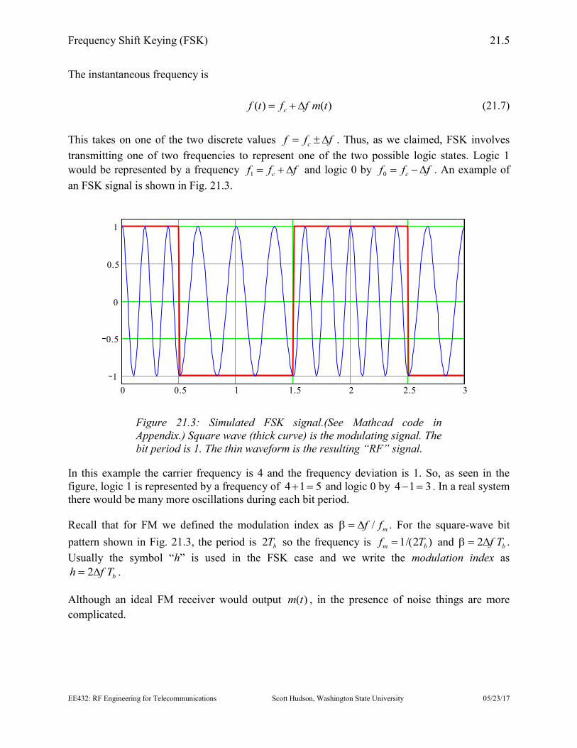
The instantaneous frequency is
)()( tmfftf c (21.7)
This takes on one of the two discrete values fff c . Thus, as we claimed, FSK involves
transmitting one of two frequencies to represent one of the two possible logic states. Logic 1
would be represented by a frequency fff c 1 and logic 0 by fff c 0 . An example of
an FSK signal is shown in Fig. 21.3.
0 0.5 1 1.5 2 2.5 3
1
0.5
0
0.5
1
0 0.5 1 1.5 2 2.5 3
1
0.5
0
0.5
1
Figure 21.3: Simulated FSK signal.(See Mathcad code in
Appendix.) Square wave (thick curve) is the modulating signal. The
bit period is 1. The thin waveform is the resulting “RF” signal.
In this example the carrier frequency is 4 and the frequency deviation is 1. So, as seen in the
figure, logic 1 is represented by a frequency of 514 and logic 0 by 314 . In a real system
there would be many more oscillations during each bit period.
Recall that for FM we defined the modulation index as mff / . For the square-wave bit
pattern shown in Fig. 21.3, the period is bT2 so the frequency is )2/(1 bm Tf and bTf 2 .
Usually the symbol “h” is used in the FSK case and we write the modulation index as
bTfh 2 .
Although an ideal FM receiver would output )(tm , in the presence of noise things are more
complicated.

Frequency Shift Keying (FSK) 21.6
EE432: RF Engineering for Telecommunications Scott Hudson, Washington State University 05/23/17
BER for FSK
In general, to demodulate an FSK signal and recover the modulation )(tm , we need to determine
at which of the frequencies 10 , ff there is more power present during a given bit period. Ideally
all the power would be at one or the other frequency and then we would know which logic state
was being sent. However, we are doing this in the presence of noise. With noise it is possible that
more power will appear at the wrong frequency than at the right one, and we will have a bit
error. We want to figure out how often this happens.
Mathematically, we can take the approach we use to calculate Fourier series coefficients,
namely, multiply by a sinusoid and integrate. This can be implemented in hardware using mixers
and integrators. Assume a logic “1” is being sent. The received signal will be tAc 1cos for a
period Tb. The receiver adds noise to give us a total signal of )(cos 1 tntAc . Now calculate the
Fourier coefficient at 1 . We get
1
0
1
0
111
cos)(2
cos)(cos2
XA
dtttnT
A
dtttntAT
a
c
T
b
c
T
c
b
b
b
(21.8)
The second term X1 is the Fourier coefficient of t1cos for the noise. We assume this is a zero-
mean Gaussian random variable. Since the time interval is bT , spectral components within a
bandwidth of bTB /1 will contribute to this. This corresponds to a noise power of BN0 where
NkTN 0 is the noise spectral density. Therefore, the variance is bTNBNX /00
2
1 . Now
let’s calculate the Fourier coefficient at 0 . We get
0
0
0
0
010
cos)(2
cos)(cos2
X
dtttnT
dtttntAT
a
b
b
T
b
T
c
b
(21.9)
Here we’ve assumed that t1cos and t0cos are orthogonal over this interval. This sets a
constraint on the difference of the two frequencies, as we’ll see later. X0 is another Gaussian
random variable with variance bTN /0 .

Frequency Shift Keying (FSK) 21.7
EE432: RF Engineering for Telecommunications Scott Hudson, Washington State University 05/23/17
If 01 aa then we conclude, correctly, that the logic level is “1”. Otherwise we make a bit error.
Equivalently, we look at 01 aar . If this is positive then we assume logic level “1” while if it
is negative we assume logic level “0”. Now 01 XXAr c . 10 , XX are both zero-mean
Gaussian RVs with variance bTN /0 . If they are independent, then statistical theory tells us that
their difference with also be a zero-mean Gaussian RV with variance bTN /2 0
2 . Therefore r
will be a Gaussian RV with mean cA and variance bTN /2 0
2 as illustrated in Fig. 21.1.
Ac
r
p(r)
Figure 21.4: PDF of FSK detector output.
We make an error in figuring out the logic state if 0r . The probability of this is
c
Ar
e
AQ
drePc0
2
12
2
1
(21.10)
If the logic state had been “0”, we’d get the mirror image of Fig. 21.1 and find the same error.
Therefore (21.10) is the BER.
Let’s express /cA in a couple of different ways to get some insight into this expression. Using
bTN /2 0
2 and 2/2
bcb TAE , we can write 00
22 /2/)/( NENTAA bbcc , so
0N
EQP b
e (21.11)
This is plotted in Fig. 21.5. Given a receiver noise temperature, NkTN 0 is determined, and this
expression tells us the received energy per bit required to achieve a given BER. For example,
from Fig. 21.5 we can see that to get a BER of about 310 we’d need 0/ NEb to be about 10 dB.

Frequency Shift Keying (FSK) 21.8
EE432: RF Engineering for Telecommunications Scott Hudson, Washington State University 05/23/17
The fact that 0/ NEb determines the BER has implications for our bit rate bb TR /1 . With a
fixed 0N we need to keep bE fixed to maintain a given BER. But bWRbWRb RPTPE /,, . So, if
we increase our bit rate, we must increase received power by the same amount. Conversely, if
received power decreases, we can maintain our BER by reducing the bit rate. So, the data rate
your radio link will operate at is an important consideration in determining the required received
power.
Recall that for a bandwidth of bTB /1 and a noise spectral density NkTN 0 , the noise power
is BNP WN 0, . Now
WN
WR
WR
bWRb
P
P
BN
P
N
TP
N
E
,
,
0
,
0
,
0
(21.12)
That is, 0/ NEb is also the S/N ratio. However, since the noise power depends on the bandwidth,
which depends on the data rate, 0/ NEb is in a sense a more fundamental quantity.

Frequency Shift Keying (FSK) 21.9
EE432: RF Engineering for Telecommunications Scott Hudson, Washington State University 05/23/17
0 2 4 6 8 10 12 14 16-9
-8
-7
-6
-5
-4
-3
-2
-1
0
Eb/N0 (dB)
FSK: log(BER) vs. Eb/N0
coherentincoherent
Figure 21.5: BER vs. 0/ NEb . Solid blue curve corresponds to
coherent detection; dashed red curve corresponds to incoherent
detection.
In writing (21.8) and (21.9) we’ve implicitly assumed that the cosine in the signal and the cosine
in our detector had the same phase. This kind of detection scheme we’ve outlined is a coherent
scheme. If you can’t get phase coherence, you have to use a noncoherent detector. For example,
you could compare the amplitudes of the output of two bandpass filters, one tuned to 0f and the
other to 1f . The analysis is more difficult than for the coherent case. The result is
02
2
1 N
E
e
b
eP
(21.13)
This is also plotted in Fig. 21.5. You can see that the BER is higher than for the coherent
detector. Typically, however, less than 1 dB of increase in signal power will make up the
difference.

Frequency Shift Keying (FSK) 21.10
EE432: RF Engineering for Telecommunications Scott Hudson, Washington State University 05/23/17
FSK Spectrum
To signal a sequence of logic states, we are sending a series of pulses of the form (21.1) each
with frequency fff c 0 or fff c 1 . The spectrum of a single pulse is given by (21.2).
We might be inclined to think that the power spectrum of an FSK signal would therefore consist
of two squared sincs, one centered at f0 and one at f1. This is more-or-less true if the frequency
deviation is greater than or about equal to the width of one sinc, namely, bT/1 . For the waveform
shown in Fig. 21.3, the power spectrum is as shown in Fig. 21.6
0 1 2 3 4 5 6 7 860
50
40
30
20
10
0
Figure 21.6: Power spectrum of the FSK signal shown in Fig.
21.3. Power in dB vs. frequency.
For this situation we can estimate the bandwidth as the difference of the frequencies f0 and f1,
which is f2 , plus half the width of the lower sinc, plus half the width of the upper sinc, i.e.,
bTfB /12 (21.14)
For the situation illustrated in Fig. 21.6, this would be 3. Or we can use Carson’s rule
)(2 mffB . In this case we have to realize that if our bits are flipping back and forth
between –1 and 1, then )(tm has a period of 2Tb, corresponding to a frequency of bm Tf 2/1 .
Putting this into Carson’s rule gives (21.14).
So, we see that our BER is given by (21.11) and our bandwidth by (21.14). Since the BER
doesn’t (apparently) depend on B, why not let 0f so that we only need to use a bandwidth
bT/1 ? Clearly something must be in our way, because 0f would mean that there would be
no modulation and hence no information being sent.

Frequency Shift Keying (FSK) 21.11
EE432: RF Engineering for Telecommunications Scott Hudson, Washington State University 05/23/17
MSK & GMSK
What is the minimum bandwidth (21.14) that we can use for FSK? Implicit in (21.9) is the
orthogonality of t0cos and t1cos :
0
2)(sinc2)(sinc
)(
)sin(
)(
)sin(
)cos(1
)cos(1
coscos2
0101
01
01
01
01
0
01
0
010
0
1
bb
b
b
b
b
T
b
T
b
T
b
TffTff
T
T
T
T
dttT
dttT
tdttT
bbb
(21.15)
The first term is zero (or extremely close) because 01 ff is very large. For the second term to
be zero, however, we require bTff 2)( 01 to be at least 1. Since fff 201 , this means
4
4
1
b
b
R
Tf
(12.16)
that is, the frequency deviation must be at least one-fourth the bit rate. This defines the minimum
frequency deviation that results in orthogonal signals. FSK with this frequency deviation is
referred to as minimum shift keying or MSK. For MSK we have bTff 2/101 and the
modulation index is 2/1h . Therefore, during a period Tb, t1cos will go through an extra ½
of a sine wave compared to t0cos . An example of an MSK signal is shown in Fig. 21.7.

Frequency Shift Keying (FSK) 21.12
EE432: RF Engineering for Telecommunications Scott Hudson, Washington State University 05/23/17
0 0.5 1 1.5 2 2.5 3
1
0.5
0
0.5
1
0 0.5 1 1.5 2 2.5 3
1
0.5
0
0.5
1
Figure 21.7: Simulated Minimum Shift Keying (MSK) signals. At
the top is “unfiltered” MSK. At the bottom is “filtered” GMSK.
The “two-sincs” picture of the power spectrum breaks down when f gets less than about
bT/1 because the sincs overlap. The theoretical, unfiltered MSK power spectrum is
2
22
2
1))(4(
))(2cos(16)(
Tff
TfffS
c
c (12.17)
This is shown in Fig. 21.8 (boxes) along with numerical results for the waveform of Fig. 21.7.

Frequency Shift Keying (FSK) 21.13
EE432: RF Engineering for Telecommunications Scott Hudson, Washington State University 05/23/17
0 1 2 3 4 5 6 7 860
50
40
30
20
10
0
Figure 21.8: MSK and GMSK power spectra, simulation and
theory. Boxes/red curve is unfiltered MSK spectrum. Circles/blue
curve is GMSK. Dotted magenta curves are theoretical spectra.
As can be seen in Fig. 21.3, in an FSK waveform there is a sharp transition from one frequency
to the next. Rapid transitions generally require a wider bandwidth than smooth transitions. As a
result, filtering the modulation )(tm can reduce the MSK bandwidth because the transmitter will
smoothly vary between the two frequencies. This is illustrated at the bottom of Fig. 21.7. The
corresponding spectrum is shown in Fig. 21.8.
Fitlering )(tm with a Gaussian impulse response results in multiplying the MSK spectrum by a
Gaussian frequency response. If the impulse reponse is
2
)(
t
eth (21.18)
the spectrum is multiplied by
2
)()( cff
efH
(21.19)
The result is called Gaussian Minimum Shift Keying, or GMSK. The parameter determines the
bandwidth – a larger value results in smaller bandwidth. The case shown in Fig. 21.8 has
1 . The GSM digital cellular standard uses 2 . Although GMSK reduces the bandwidth, it
also increases the BER somewhat because the signal no longer spends a full Tb at either of the
two frequencies f0 or f1.

Frequency Shift Keying (FSK) 21.14
EE432: RF Engineering for Telecommunications Scott Hudson, Washington State University 05/23/17
References
1. Anderson, J. B., Digital Transmission Engineering, IEEE Press, 1999, ISBN 0-13-
082961-7.
2. Burr, A., Modulation and Coding for Wireless Communications, Prentice Hall, 2001,
ISBN 0-201-39857-5.
Appendix
The following is the Matcad code used to generate most of the figures in the text.
FSK Simulation
Bit period, carrier frequency, and frequency deviat ion constant:
T 1 fc4
T kf
4
4 T
unfiltered square-wave modulation: m0 t( ) sign cos t
T
"filtered" modulat ion: m1 t( ) cos t
T
FM signals: s0 t( ) cos 2 fc t 2kf
0
t
xm0 x( )
d
s1 t( ) cos 2 fc t 2kf
0
t
xm1 x( )
d
These are periodic, even functions with period 2T, Fourier coefficients are:
n 1 16
a0n2
2TT
T
ts0 t( ) cos2
2Tn t
d a1n2
2TT
T
ts1 t( ) cos2
2Tn t
d