freight-truck-pavement interaction, logistics, and ...freight-truck-pavement interaction, logistics,...
TRANSCRIPT
December 2012Research Report: UCPRC-RR-2012-06
Freight-Truck-Pavement Interaction,
Logistics, and Economics: Final Phase 1 Report (Tasks 1–6)
Authors:Wynand J.vdM. Steyn, Nadia Viljoen, Lorina Popescu, and Louw du Plessis
Work Conducted Under Partnered Pavement Research Program (PPRC) Strategic Plan Element 4.44: Pilot Study Investigating the Interaction and Effects for State Highway
Pavements, Trucks, Freight, and Logistics
Rev. Oct. 2014
PREPARED FOR: California Department of Transportation Division of Transportation Planning (DOTP) Office of Materials and Infrastructure
PREPARED BY:
University of PretoriaUniversity of California
Pavement Research CenterUC Davis and UC Berkeley

(This page blank)

UCPRC-RR-2012-06 i
DOCUMENT RETRIEVAL PAGE Research Report No.:
UCPRC-RR-2012-06Title: Freight-Truck-Pavement Interaction, Logistics, and Economics: Final Phase Report (Tasks 1–6) Authors: W.Jvd.M. Steyn, N. Viljoen, L. Popescu, L. du Plessis Caltrans Technical Leads: Nerie Rose Agacer-Solis and Bill Nokes Prepared for: California Department of Transportation Division of Transportation Planning (DOTP) Office of Materials and Infrastructure
FHWA No.: CA132482A
Date Work Submitted:
December 2012
Date:December 2012
Strategic Plan Element No.: 4.44
Status: Stage 6, final version
Version:Final,
revised Oct. 2014 Abstract: The intention of the study is to demonstrate the potential economic effects of delayed road maintenance and management, leading to deteriorated ride quality and subsequent increased vehicle operating costs, vehicle damage, and freight damage.
The overall objectives of this project are to enable Caltrans to better manage the risks of decisions regarding freight and the management and preservation of the pavement network, as the potential effects of such decisions (i.e., to resurface and improve ride quality earlier or delay such a decision for a specific pavement) will be quantifiable in economic terms. This objective will be reached through applying the principles of vehicle-pavement interaction (V-PI) and state-of-the-practice tools to simulate and measure peak loads and vertical acceleration of trucks and their freight on a selected range of typical pavement surface profiles on the State Highway System (SHS) for a specific region or Caltrans district.
The objectives of this report are to provide information on Tasks 1–6, and to provide guidance about the specific corridor or district on which the remainder of the study (Tasks 7–12) should be focused.
Conclusions The following conclusions are drawn based on the information provided and discussed in this report:
Ample information exists to enable the objectives of this pilot study to be met through analyzing the V-PI and logistics situation in a selected corridor in California.
The San Joaquin Valley corridor is a major production and transportation corridor in California and well-suited to serve as a pilot area for the purposes of this project.
Recommendations The following recommendations are made based on the information provided and discussed in this report:
The San Joaquin Valley should be targeted as the pilot study area for the purposes of the remaining tasks in this pilot project.
Routes I-5, SR 58, and SR 99 are recommended as suitable routes for the pilot field study. The work anticipated for Tasks 7–12 should commence once this report has been accepted and approved by the
client. Keywords: Vehicle-pavement interaction, freight transport industry sustainability and competitiveness, pavement roughness, economic evaluation, Cal-B/C, logistics Proposals for Implementation: This final Phase 1 report will be studied by the client and decisions regarding the remainder tasks of the project will be based on the outcome of this report.

ii UCPRC-RR-2012-06
Related Documents: W.J.vdM. Steyn. 2013. Freight-Truck-Pavement Interaction, Logistics, and Economics: Final Phase 1 Report
(Tasks 7–8). Research Report prepared for Caltrans Division of Transportation Planning. (UCPRC-RR-2013-08) W.J.vdM. Steyn and L. du Plessis. 2013. Freight-Truck-Pavement Interaction, Logistics, & Economics: Final Phase 1
Report (Tasks 9–11). Research Report prepared for Caltrans Division of Transportation Planning. (UCPRC-RR-2014-01)
W.J.vdM. Steyn, L. du Plessis, N. Viljoen, Q. van Heerden, L. Mashoko, E. van Dyk, and L. Popescu. 2014. Freight-Truck-Pavement Interaction, Logistics, & Economics: Final Executive Summary Report. Summary Report prepared for Caltrans Division of Transportation Planning. (UCPRC-SR-2014-01)
N. Viljoen, Q. van Heerden, L. Popescu, L. Mashoko, E. van Dyk, and W. Bean. Logistics Augmentation to the Freight-Truck-Pavement Interaction Pilot Study: Final Report 2014. Research Report prepared for Caltrans Division of Transportation Planning.(UCPRC-RR-2014-02)
Signatures
W.J.vdM. Steyn First Author
Nerie Rose Agacer-Solis
Bill Nokes Technical Reviewers
W.J.vdM. Steyn John T. Harvey Principal Investigator
Nerie Rose Agacer-Solis
Bill Nokes Caltrans Technical Leads
T. Joe Holland Caltrans Contract Manager
UCPRC-RR-2012-06 iii
TABLE OF CONTENTS
LIST OF FIGURES .............................................................................................................................................. vi
LIST OF TABLES .............................................................................................................................................. viii
DISCLAIMER STATEMENT ............................................................................................................................ ix
ACKNOWLEDGMENTS ................................................................................................................................... ix
PROJECT OBJECTIVES .................................................................................................................................... x
EXECUTIVE SUMMARY .................................................................................................................................. xi
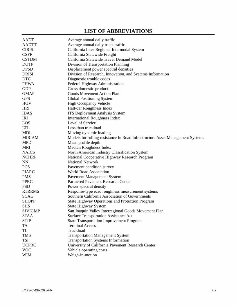
LIST OF ABBREVIATIONS ............................................................................................................................ xix
1 INTRODUCTION .......................................................................................................................................... 1
1.1 Introduction ............................................................................................................................................... 1
1.2 Background ............................................................................................................................................... 3
1.3 Scope ......................................................................................................................................................... 3
1.4 Objectives ................................................................................................................................................. 6
2 TASKS 1 AND 2 SUMMARY ........................................................................................................................ 7
2.1 Introduction ............................................................................................................................................... 7
2.2 Summary ................................................................................................................................................... 7
3 TASK 3 PROGRESS—ROAD INVENTORY ............................................................................................. 9
3.1 Introduction ............................................................................................................................................... 9
3.2 Task 3 Progress ......................................................................................................................................... 9
3.2.1Required Data ...................................................................................................................................... 9
3.2.2Ride Quality Background ..................................................................................................................... 9
3.3 Task 3 Information Resources ................................................................................................................ 15
3.3.1Caltrans PMS IRI Data....................................................................................................................... 15
3.3.2Caltrans PMS Pavement Profile Data ................................................................................................ 15
3.3.3Caltrans Routes .................................................................................................................................. 15
3.4 Task 3 Analysis ....................................................................................................................................... 28
3.5 Task 3 Outcome ...................................................................................................................................... 29
4 TASK 4 PROGRESS—VEHICLE INVENTORY ..................................................................................... 31
4.1 Introduction ............................................................................................................................................. 31
4.2 Task 4 Progress ....................................................................................................................................... 31
4.3 Task 4 Information Sources .................................................................................................................... 31
4.3.1FHWA Vehicle Classifications ........................................................................................................... 31
4.3.2California Truck Definitions and Information ................................................................................... 31
iv UCPRC-RR-2012-06
4.3.3Commodity Flow Survey ................................................................................................................... 34
4.3.4Truck Traffic Analysis Using WIM Data in California ...................................................................... 37
4.3.5Truck Route List................................................................................................................................. 40
4.3.6Truck Tire and Suspension Use .......................................................................................................... 40
4.4 Task 4 Outcome ...................................................................................................................................... 42
5 TASK 5 PROGRESS—INFORMATION REVIEW ................................................................................. 43
5.1 Introduction ............................................................................................................................................. 43
5.2 Task 5 Progress ....................................................................................................................................... 43
5.3 Task 5 Information Resources ................................................................................................................ 43
5.3.1California Statewide Freight Planning ............................................................................................... 44
5.3.2Commodity Flow Survey ................................................................................................................... 44
5.3.3San Joaquin Valley Information ......................................................................................................... 50
5.3.4Goods Movement Action Plan ........................................................................................................... 62
5.3.5California Life-Cycle Benefit/Cost Analysis Model .......................................................................... 63
5.3.6Private Industry .................................................................................................................................. 66
5.3.7MIRIAM Project ................................................................................................................................ 67
5.3.8California Inter-Regional Intermodal System .................................................................................... 68
5.3.9I-5/SR 99 Origin and Destination Truck Study .................................................................................. 68
5.3.10 State of Logistics South Africa ................................................................................................... 70
5.3.11 Other Regions and Corridors ...................................................................................................... 80
5.4 Freight Logistics Analysis ...................................................................................................................... 80
5.4.1Introduction to Freight Logistics and the Broader Supply Chain ...................................................... 80
5.4.2Freight Damage as a Result of V-PI ................................................................................................... 82
5.4.3Pilot Study Objectives ........................................................................................................................ 84
5.4.4Information Requirements to Calculate Freight Damage Costs ......................................................... 84
5.4.5Selecting a Preferable Study Area and Freight Types for the Pilot Study .......................................... 86
5.5 Links, Inputs, and Outputs ...................................................................................................................... 90
6 DISCUSSION ................................................................................................................................................ 91
6.1 Introduction ............................................................................................................................................. 91
6.2 Data Consolidation ................................................................................................................................. 91
6.2.1Introduction ........................................................................................................................................ 91
6.2.2Report Issues ...................................................................................................................................... 91
6.2.3Motivational Reasons for Recommended Region/Corridor ............................................................... 97
6.3 Vehicle Field Study Parameters .............................................................................................................. 97
UCPRC-RR-2012-06 v
6.3.1Field Work Objective ......................................................................................................................... 97
6.3.2Field Work Requirements ................................................................................................................... 98
6.3.3Route Requirements ........................................................................................................................... 99
6.3.4Experimental Design ........................................................................................................................ 101
6.3.5General Notes ................................................................................................................................... 101
6.4 Caltrans Decision .................................................................................................................................. 102
7 CONCLUSIONS AND RECOMMENDATIONS .................................................................................... 103
7.1 Conclusions ........................................................................................................................................... 103
7.2 Recommendations ................................................................................................................................. 103
8 REFERENCES ........................................................................................................................................... 105
TECHNICAL APPENDICES .......................................................................................................................... 108
APPENDIX A: MINUTES OF PROJECT KICKOFF MEETING .............................................................. 108

vi UCPRC-RR-2012-06
LIST OF FIGURES
Figure 1.1: Schematic layout and linkages between project tasks. ......................................................................... 5
Figure 3.1: Example of four typical road profiles. ................................................................................................ 10
Figure 3.2: Definition of macrotexture and microtexture of pavement surfacing aggregate (6). ........................... 11
Figure 3.3: Displacement power spectral densities (DPSDs) on ISO classification for three different
pavements. ............................................................................................................................................. 14
Figure 3.4: Caltrans District 1 routes. ................................................................................................................... 16
Figure 3.5: Caltrans District 2 routes. ................................................................................................................... 17
Figure 3.6: Caltrans District 3 routes. ................................................................................................................... 18
Figure 3.7: Caltrans District 4 routes. ................................................................................................................... 19
Figure 3.8: Caltrans District 5 routes. ................................................................................................................... 20
Figure 3.9: Caltrans District 6 routes. ................................................................................................................... 21
Figure 3.10: Caltrans District 7 routes. ................................................................................................................. 22
Figure 3.11: Caltrans District 8 routes. ................................................................................................................. 23
Figure 3.12: Caltrans District 9 routes. ................................................................................................................. 24
Figure 3.13: Caltrans District 10 routes. ............................................................................................................... 25
Figure 3.14: Caltrans District 11 routes. ............................................................................................................... 26
Figure 3.15: Caltrans District 12 routes. ............................................................................................................... 27
Figure 4.1: California Truck Map legend for STAA routes (17). .......................................................................... 33
Figure 4.2: California Truck Map legend for California Legal routes (17). .......................................................... 33
Figure 4.3: Average annual daily traffic (AADT) data for 12 Caltrans districts. .................................................. 36
Figure 4.4: Percentage trucks data for 12 Caltrans districts. ................................................................................. 36
Figure 4.5: AADT and percentage trucks data for Caltrans counties (=AADT; × = % Trucks). ........................ 37
Figure 4.6: Distribution of WIM stations on California state highway network in March 2001. ......................... 39
Figure 5.1: Schematic of how the various transportation models are being developed ........................................ 43
Figure 5.2: Key regional truck routes in the San Joaquin Valley (24). ................................................................. 52
Figure 5.3: Inbound, outbound, and internal commodity distribution, 2007 (24). ................................................ 53
Figure 5.4: Outbound commodities from the San Joaquin Valley (24) ................................................................. 54
Figure 5.5: Inbound commodities from the San Joaquin Valley (24). ................................................................... 54
Figure 5.6: Priority regions and corridors in California (29). ............................................................................... 63
Figure 5.7: Cal-B/C framework. ........................................................................................................................... 64
Figure 5.8: Cal-B/C graphical user interface. ....................................................................................................... 65
Figure 5.9: Potential effects of deteriorating road quality on the broader economy. ............................................ 70
Figure 5.10: Potential increase in vehicle maintenance and repair cost due to bad roads. .................................... 73
UCPRC-RR-2012-06 vii
Figure 5.11: Typical damage to fresh produce cargo due to road roughness. ....................................................... 74
Figure 5.12: Comparison between dominant frequencies experienced by fruit cargo and the vibration range that
results in damage. .................................................................................................................................. 77
Figure 5.13: Normalized distributions of the vertical accelerations experienced within pallets at various packing
levels at the front of the truck. ............................................................................................................... 78
Figure 5.14: Simplified schematic of a supply chain. ........................................................................................... 82
Figure 5.15: Comparison of different commodity shipments originating from California. (See Table 5.12 for
description of index designations in this figure.) .................................................................................. 87
Figure 5.16: Comparison of different commodity shipments on truck in California. ........................................... 88
Figure 6.1: Distribution of average ride qualities on routes identified in Table 6.1. ........................................... 100
Figure 6.2: Typical location of accelerometers on typical South African truck. ................................................. 100
viii UCPRC-RR-2012-06
LIST OF TABLES
Table 1.1: Task Description for Project ................................................................................................................... 4
Table 3.1: ISO (15) Classification and IRI and HRI Values for Three Typical Pavement Sections ...................... 14
Table 3.2: Typical Road Profile Information from PMS Database ....................................................................... 15
Table 3.3: Number of Sections and Lane-Miles of Sections for Which Data Ride Quality Exist in the Current
PMS Database, by District .................................................................................................................... 28
Table 3.4: Number of Sections and Lane-Miles of Sections for Which Ride Quality Data Exist in the Current
PMS Database, by County .................................................................................................................... 29
Table 4.1: FHWA Vehicle Classes with Definitions (18) ...................................................................................... 32
Table 4.2: Most Common Truck Types in California Used for Transporting Goods ............................................ 34
Table 4.3: 2010 Truck Count Data Example (19) ................................................................................................. 35
Table 4.4: Summarized Analysis of Truck Count Data per District (19) .............................................................. 35
Table 4.5: Summary of Basic Information for Each WIM Station in California (20) ........................................... 37
Table 4.6: Example Data from Truck Route List.xlsx ........................................................................................... 41
Table 4.7: Summary of Typical Advisories and Restrictions on Caltrans Network .............................................. 41
Table 5.1: Summarized Shipment Characteristics by Mode of Transportation for State of
Origin—California (23) ......................................................................................................................... 47
Table 5.2:Summary of Freight Descriptions (for NAICS Industries) Transported in 2007—All Trucks ............. 48
Table 5.3: Major Highway Corridors and Proportion of Truck Traffic, San Joaquin Valley (24) ......................... 53
Table 5.4: Outbound Commodity Movements, by County (tons) (24) ................................................................. 56
Table 5.5: Inbound Commodity Movements, by County (tons) (24) .................................................................... 56
Table 5.6: Top Agricultural Producing Counties in San Joaquin Valley (26) ........................................................ 57
Table 5.7: Potential Increase in Vehicle Damage Cost under Deteriorating Road Conditions .............................. 71
Table 5.8: Summary of Vehicle Maintenance and Repair Cost for Routes with Different IRIs ............................ 72
Table 5.9: Summary of Potential Increases due to Worsening Road Conditions .................................................. 73
Table 5.10: Benefit-Cost Ratio of Keeping the Road in a Good Condition .......................................................... 76
Table 5.11: Comparison of Average Wheat Loss on Good and Bad Roads .......................................................... 80
Table 5.12: Commodity Classes Associated with Figure 5.15 .............................................................................. 87
Table 5.13: Commodity Types Associated with Figure 5.16 ................................................................................. 89
Table 6.1: Potential Routes for Field Measurements ............................................................................................ 99
Table 6.2: Experimental Design for Pilot Study .................................................................................................. 101
UCPRC-RR-2012-06 ix
DISCLAIMER STATEMENT
This document is disseminated in the interest of information exchange. The contents of this report reflect the
views of the authors, who are responsible for the facts and accuracy of the data presented herein. The contents do
not necessarily reflect the official views or policies of the State of California or the Federal Highway
Administration. This publication does not constitute a standard, specification, or regulation. This report does not
constitute an endorsement by the California Department of Transportation (Caltrans) of any product described
herein.
For individuals with sensory disabilities, this document is available in braille, large print, audiocassette, or
compact disk. To obtain a copy of this document in one of these alternate formats, please contact: the California
Department of Transportation, Division of Research, Innovation, and Systems Information (DRISI), MS 83,
P.O. Box 942873, Sacramento, CA 94273 0001.
ACKNOWLEDGMENTS
The input and comments of all organizations contacted for information in this project are acknowledged.
Specifically, the input of the following persons are acknowledged:
Caltrans technical advisors to the project team: Al Arana (DOTP Office of System Planning), Joanne
McDermott (DOTP Office of Freight Planning)
DOTP Economic Analysis Branch staff: Nerie Rose Agacer-Solis, Barry Padilla, and Austin Hicks
Division of Research, Innovation and System Information (DRISI) Office of Materials and Infrastructure:
Joe Holland and Bill Nokes
x UCPRC-RR-2012-06
PROJECT OBJECTIVES
The overall objectives of this project are to enable Caltrans to better manage the risks of decisions regarding
freight and the management and preservation of the pavement network, as the potential effects of such decisions
(i.e., to resurface and improve ride quality earlier or delay such a decision for a specific pavement) will be
quantifiable in economic terms. This objective will be reached through applying the principles of
vehicle-pavement interaction (V-PI) and state-of-the-practice tools to simulate and measure peak loads and
vertical acceleration of trucks and their freight on a selected range of typical pavement surface profiles on the State
Highway System (SHS) for a specific region or Caltrans district.
The objectives of this report are to provide information on Tasks 1–6, and to provide guidance about the specific
corridor or district on which the remainder of the study (Tasks 7–12) should be focused.
Note: This document reports information that was developed and provided incrementally by the research team as
the pilot study proceeded. For consistency with the incremental nature of the work and the reporting on it, this
final report retains the same grammatical tense referring to remaining tasks (as yet to be done), although all tasks
and the pilot study have been completed.

UCPRC-RR-2012-06 xi
EXECUTIVE SUMMARY
Introduction
This pilot study applies the principles of vehicle-pavement interaction (V-PI) and state-of-the-practice tools to
simulate and measure peak loads and vertical acceleration of trucks and their freight on a selected range of typical
pavement surface profiles on the State Highway System (SHS) for a specific region or Caltrans district. The pilot
study is not focusing on the detailed economic analysis of the situation; however, the outputs from the pilot study
are expected to be used as input or insights by others toward planning and economic models to enable an improved
evaluation of the freight flows and costs in the selected region/district. It is anticipated that use of findings from
this study as input by others into planning and economic models will enable calculating the direct effects of ride
quality (and therefore road maintenance and management efforts) on the regional and state economy.
The final product of this pilot study will consist of data and information resulting from (1) simulations and
measurements, (2) tracking truck/freight logistics (and costs if available), and (3) input for economic evaluation
based on V-PI and freight logistics investigation. Potential links of the data and information to available and
published environmental emissions models (e.g., greenhouse gas [GHG], particulate matter), pavement
construction specifications, and roadway maintenance/preservation will be examined.
The intention of the pilot study is to enable economic evaluation (using tools such as Caltrans’ Cal-B/C model) of
the potential economic effects of delayed road maintenance and management, leading to deteriorated ride quality
and subsequent increased vehicle operating costs, vehicle damage, and freight damage. The study will be
conducted as a pilot study in a region or Caltrans district where the probability of collecting the maximum data on
road quality, vehicle population, and operational conditions will be the highest and where the outcomes of the
study may be incorporated into economic and planning models. The final selection of the region/district will be
made based on information collected during Tasks 3–5; the final selection of an appropriate region/district will be
made by Caltrans. This focused pilot study enables the approach to be developed and refined in a contained
region/district where ample access may be available to required data, information, and models. After the pilot
study is completed and the approach has been accepted and shown to provide benefits to Caltrans and stakeholders,
it can be expanded to other regions/districts as required.
The overall objectives of this project are to enable Caltrans to better manage the risks of decisions regarding
freight and the management and preservation of the pavement network, as the potential effects of such decisions
(i.e., to resurface and improve ride quality earlier or delay such a decision for a specific pavement) will be
quantifiable in economic terms. This objective will be reached through applying the principles of
vehicle-pavement interaction (V-PI) and state-of-the-practice tools to simulate and measure peak loads and

xii UCPRC-RR-2012-06
vertical acceleration of trucks and their freight on a selected range of typical pavement surface profiles on the State
Highway System (SHS) for a specific region or Caltrans district.
The objectives of this report are to provide information on Tasks 1–6, and to provide guidance about the specific
corridor or district on which the remainder of the pilot study (Tasks 7–12)should be focused.
The data presented and discussed in Sections 3 to 5 of this document presents information sourced from a range of
independent sources. Each of the sets of information is discussed in detail as individual information. Relevant
information originating from Sections 3 to 5 is combined to present a case for a specific region/corridor to be
focused on. The details of the specific data sets are not necessarily repeated, but reference is made to the relevant
sources and locations in the report.
Report Issues
The purpose of this pilot study is to provide data and information that will provide input supporting Caltrans’
freight program plans and legislation-mandated requirements with findings potentially contributing to economic
evaluations; identification of challenges to stakeholders; and identification of problems, operational concerns, and
strategies that “go beyond the pavement”—including costs to the economy and the transportation network (delay,
packaging, environment, etc.). Findings could lead to improved pavement policies and practices, such as strategic
recommendations that link pavement surface profile, design, construction, and preservation with V-PI. These
findings should also provide information for evaluating the relationship between pavement ride quality (stemming
from the pavement’s condition), vehicle operating costs, freight damage, and logistics.
Road Inventory
The main outcome of Task 3 is to identify routes in each district and county for which ride quality data exists, as
well as the actual ride quality for these routes (due to the volume of data, the actual data are kept only in electronic
form). Routes in California have been identified and a database containing actual road profiles and ride quality
data is available for use in the remainder of the pilot project.
Vehicle Inventory
The deliverable for Task 4 is a table of current vehicle population per standard FHWA vehicle classifications for
Caltrans. Based on the various sources used in this task (FHWA truck classifications, commodity flow analysis,
and weigh-in-motion [WIM] data), the following was identified:
The most common truck types in the pilot study area are FHWA Class 9 and 12 (up to 48 percent of the
trucks on selected routes), followed by Class 5.

UCPRC-RR-2012-06 xiii
High truck flows are experienced in District 6, part of the San Joaquin Valley.
Axle load spectra are heavier at night than in the daytime.
Axle load spectra and truck type distribution show very little seasonal variation.
Axle load spectra are much higher in the Central Valley than in the Bay Area and Southern California,
particularly for tandem axles.
More than 90 percent of the truck traffic traveled in the outside or two outside lanes (two- or three-lane [in
one direction] highways) or two outside (three-lane [in one direction] highways) lanes.
Truck speeds typically fall within the range of 50 to 75 mph (80 to 120 km/h).
Leaf springs are predominantly used in steering axles, with drive axles using air suspension and trail axles
using leaf suspension.
Information Review
Task 5 focuses on evaluating the data obtained from the various resources for Tasks 3–4, as well as additional
relevant information that may add to the project. The deliverable of Task 5 is a detailed understanding and input to
the progress report on the available data sources and required analyses for the project, inclusive of indications of
the potential links between the outputs from this project and the inputs for the various economic and planning
models.
California Statewide Freight Planning
The purpose of the California Statewide Freight Forecast (CSFF) model is to provide a policy-sensitive model to
forecast commodity flows and commercial vehicle flows within California, addressing socioeconomic conditions,
land-use policies related to freight, environmental policies, and multimodal infrastructure investments.
Appropriate information and data about freight movements and costs are needed to enable accurate modeling.
Commodity Flow Survey
It is evident that truck-based transportation dominates the freight transportation scene in California.
Eighty-two percent of the freight tons shipped from California utilizes only trucks. The data indicate that the
highest percentage of commodities (in terms of value, tons, and ton-miles) transported by truck consists of
manufacturing goods, wholesale trade, and nondurable goods for the whole of California. No specific information
for commodity flows into California (destination California) could be identified in this pilot study.
San Joaquin Information
The San Joaquin Valley is composed of eight counties and 62 cities. It has a diverse internal economy and also
plays a major role in the distribution of agricultural materials throughout California, the United States, and the
world. Trucks are the dominant mode, with more than 450 million tons of goods moved by truck into, out of, or
xiv UCPRC-RR-2012-06
within the San Joaquin Valley in 2007—more than 85 percent of all tonnage associated with these types of moves
in the San Joaquin Valley. Truck movement in the San Joaquin Valley relies on a combination of all levels of
highways and roads in the area. Key regional highways include the primary north-south corridors (I-5 and SR 99)
and east-west corridors (I-580, SR 152, SR 41, SR 46, and SR 58), which in total constitute more than 31,000
lane-miles. There are over 2,700 lane-miles of truck routes in the San Joaquin Valley region, with over 80 percent
designated as national STAA Truck Routes.
Farm products are the dominant commodity carried outbound from the San Joaquin Valley, comprising 33 percent
of the total outbound movements. These consist of fresh field crops (vegetables, fruit and nuts, cereal grains, and
animal feed). Stone and aggregates account for 18 percent of the total, food and tobacco products around
10 percent, and waste and mixed freight 6 percent and 4 percent of the total tonnage, respectively.
The region accounts for over 8 percent of the total gross domestic product (GDP) for California. However, the
region accounts for a much higher proportion of output within sectors such as agriculture (nearly 50 percent) and
mining and mineral extraction (25 percent). The San Joaquin Valley includes 6 of the top 10 counties in California
in total value of agricultural production.
Goods Movement Action Plan
California’s Goods Movement Action Plan (GMAP) includes a compiled inventory of existing and proposed
goods movement infrastructure projects, including previously identified projects in various regional
transportation plans and transportation improvement programs prepared by metropolitan planning organizations,
regional transportation planning agencies, and county transportation commissions. One of the four priority regions
and corridors identified in the GMAP is the Central Valley region, which coincides with the San Joaquin Valley.
California Life-Cycle Benefit/Cost Analysis Model
Caltrans uses the California Life-Cycle Benefit/Cost Analysis Model (Cal-B/C) to conduct investment analyses of
projects proposed for the interregional portion of the State Transportation Improvement Program (STIP), the State
Highway Operations and Protection Program (SHOPP), and other ad hoc analyses requiring benefit-cost analysis.
The following required inputs are deemed to be potentially affected by the work conducted in this pilot study:
roadway type, number of general traffic lanes, number of HOV lanes, HOV restriction, highway free-flow speed,
current and forecast average annual daily traffic (AADT), hourly HOV/HOT volumes, percent trucks, truck speed,
and pavement condition.

UCPRC-RR-2012-06 xv
Industry
Potential involvement of industry in Task 8 activities includes:
GPS tracking and acceleration measurements on selected trucks traveling on designated State Highway
segments—need for trucks, trailers and freight
Truck trailer information as input into computer simulations of vehicles traveling over a range of
pavements
Models for Rolling Resistance in Road Infrastructure Asset Management Systems Project
The objective of the Models for rolling resistance In Road Infrastructure Asset Management systems (MIRIAM)
project is to conduct research to provide sustainable and environmentally friendly road infrastructure, mainly
through reducing vehicle rolling resistance, and subsequently lowering CO2 emissions and increasing energy
efficiency. Potential links between the MIRIAM project and the pilot study mainly lie in the possible use of
selected rolling resistance models originating from MIRIAM in the evaluation of the effects of pavement
roughness on vehicle energy use, emissions, and rolling resistance. Caltrans and UCPRC have participated in
MIRIAM Phase I and plan to continue participating in Phase II. Initial MIRIAM studies indicated that:
Rolling resistance is a property of tires and the pavement surface.
A proposed source model for the pavement influence on rolling resistance contains mean profile depth
(MPD), pavement roughness (IRI), and pavement stiffness as significant pavement parameters.
For light vehicles the effect of pavement roughness on rolling resistance is probably around a third of the
effect of MPD, and it appears to be higher for heavy vehicles.
California Inter-Regional Intermodal System
The California Inter-Regional Intermodal System (CIRIS) was envisioned as an umbrella concept for rail
intermodal service to and from the Port of Oakland and other Northern California locations. The increased use of
rail options for these transportation options will affect truck volumes and deterioration of the pavement
infrastructure.
I-5/SR 99 Origin and Destination Truck Study
This study indicated that:
Traffic volumes within the study area were found to be consistent for fall and spring seasons, with the
some exceptions, whereas overall truck percentages were higher in spring compared to fall, with a few
exceptions.
Little variance was observed in truck travel patterns between fall and spring.
The majority of trucks (83.8 percent) were 5-axle double-unit type.
xvi UCPRC-RR-2012-06
Seventy percent of the trucks were based within California: 47 percent of these were based in the San
Joaquin Valley region, and 34 percent in the Southern California region.
The top five commodity types by percentage are food and similar products (21 percent), empty trucks
(18 percent), farm products (14 percent), miscellaneous freight (12 percent), and transportation
equipment (4 percent).
State of Logistics South Africa
The ride quality of a road has, for many years, been used as the primary indication of the quality of a road—mainly
due to findings that deterioration in the road structure ultimately translates into a decrease in the ride quality of the
road. Various studies about the effect of the ride quality of roads on the vibrations and responses in vehicles have
been conducted, with the main conclusions indicating that a decrease in the ride quality of a road is a major cause
of increased vibrations and subsequent structural damage to vehicles. These increased vibrations and structural
damage to vehicles potentially have many negative effects on the transportation cost of companies (including both
truckers/carriers and manufacturers/producers of goods) and the broader economy of a country.
The increase in internal logistics costs due to inadequate road conditions is experienced by most, if not all,
transportation companies. This figure eventually adds up to a massive increase in the logistics costs of a country as
a whole. As the logistics costs of a country increase, the cost of its products in the global marketplace increases,
which can have devastating effects on the global competitiveness of that country. It is therefore of critical
importance to manage logistics costs effectively and to minimize unnecessary costs that can translate into higher
product costs.
Comparing the estimated annual road maintenance costs per kilometer with the potential savings in vehicle
operating costs shows significant benefits that can be realized by keeping the road in a good condition.
The vertical acceleration experienced when traveling over rough road surfaces is what causes damage to vehicles,
increased wear and tear and, potentially, damage to and loss of transported cargo. The economic impact of
damaged agricultural cargo is absorbed differently by large- and small-scale farming companies.

UCPRC-RR-2012-06 xvii
Freight Logistics
When freight is damaged it results in both direct and indirect losses in potential revenue through effects on
logistical operations. These operational repercussions depend on the type of freight and the standard operating
procedures of shipper and receiver. They include:
Product is sent back to the shipper for replacement, repair, or repackaging—placing a burden on the
reverse supply chain.
Product is “written off” and must be disposed of by the receiver.
Product must be reclassified as damaged before selling.
The most prominent implications for the freight logistics aspect is the link to the Cal-B/C model. To perform a
benefit-cost analysis of upgrading/repairing a certain stretch of road, potential freight damage savings accrued by
the upgrade must be given as input into the Cal-B/C model. Therefore, the pilot study should develop a
methodology whereby field measurements, stakeholder engagements, and existing data sources can be used to
estimate freight damage savings along a certain stretch of road.
To achieve the objectives discussed above requires cost calculations at a disaggregate level (consisting of many
aspects, including type of goods, type and attributes of truck/trailer, and attributes of roadway). Firstly, the
expected freight damage cost incurred by a particular type of shipment must be quantified. Secondly, the
individual shipment costs must be aggregated to provide higher-level cost estimates.
Based on the available information, the following commodities should be most relevant for this pilot study:
Various kinds of manufactured goods, particularly nondurable or electronic goods
Agricultural and various other food products
Mining products, such as coal, minerals, gravel
Summary
Based on the information in Section 6.2.2, there exists a good understanding of the SHS pavement conditions in
terms of ride quality in California, as well as the major truck types and operational conditions on these pavements.
The major commodities being transported have been identified, and the potential links with models such as the
Cal-B/C models are apparent. Most of the information on commodity flows and truck operations are available for
the San Joaquin Valley, which forms a major corridor for transport of agricultural and related freight.

xviii UCPRC-RR-2012-06
Motivational Reasons for Recommended Region/Corridor
The information presented in this report provides a good basis of information to describe the freight movement
and transport infrastructure conditions in the San Joaquin Valley region in California.
Transportation and logistics in this corridor are being studied in detail in various studies, supporting the notion that
the corridor is important for the economy of California. This idea is also supported by data indicating that a large
proportion of freight originates, passes through, or is destined for companies and markets in this region.
Based on the information provided in this report, it is thus recommended that the San Joaquin Valley region be
used in the remaining tasks of this pilot study. Routes I-5, SR 58, and SR 99 are recommended as suitable routes
for the pilot field study. Specific commodities and trucks in the valley need to be identified for the details of
Tasks 7–8.
UCPRC-RR-2012-06 xix
LIST OF ABBREVIATIONS
AADT Average annual daily traffic AADTT Average annual daily truck traffic CIRIS California Inter-Regional Intermodal System CSFF California Statewide Freight CSTDM California Statewide Travel Demand Model DOTP Division of Transportation Planning DPSD Displacement power spectral densities DRISI Division of Research, Innovation, and Systems Information DTC Diagnostic trouble codes FHWA Federal Highway Administration GDP Gross domestic product GMAP Goods Movement Action Plan GPS Global Positioning System HOV High Occupancy Vehicle HRI Half-car Roughness Index IDAS ITS Deployment Analysis System IRI International Roughness Index LOS Level of Service LTL Less than truckload MDL Moving dynamic loading MIRIAM Models for rolling resistance In Road Infrastructure Asset Management Systems MPD Mean profile depth MRI Median Roughness Index NAICS North American Industry Classification System NCHRP National Cooperative Highway Research Program NN National Network PCS Pavement condition survey PIARC World Road Association PMS Pavement Management System PPRC Partnered Pavement Research Center PSD Power spectral density RTRRMS Response-type road roughness measurement systems SCAG Southern California Association of Governments SHOPP State Highway Operations and Protection Program SHS State Highway System SJVIGMP San Joaquin Valley Interregional Goods Movement Plan STAA Surface Transportation Assistance Act STIP State Transportation Improvement Program TA Terminal Access TL Truckload TMS Transportation Management System TSI Transportation Systems Information UCPRC University of California Pavement Research Center VOC Vehicle operating costs WIM Weigh-in-motion
xx UCPRC-RR-2012-06
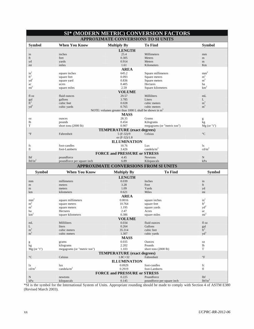
SI* (MODERN METRIC) CONVERSION FACTORS APPROXIMATE CONVERSIONS TO SI UNITS
Symbol When You Know Multiply By To Find Symbol LENGTH
in inches 25.4 Millimeters mm ft feet 0.305 Meters m yd yards 0.914 Meters m mi miles 1.61 Kilometers Km
AREAin2 square inches 645.2 Square millimeters mm2 ft2 square feet 0.093 Square meters m2 yd2 square yard 0.836 Square meters m2 ac acres 0.405 Hectares ha mi2 square miles 2.59 Square kilometers km2
VOLUMEfl oz fluid ounces 29.57 Milliliters mL gal gallons 3.785 Liters L ft3 cubic feet 0.028 cubic meters m3 yd3 cubic yards 0.765 cubic meters m3
NOTE: volumes greater than 1000 L shall be shown in m3
MASSoz ounces 28.35 Grams g lb pounds 0.454 Kilograms kg T short tons (2000 lb) 0.907 megagrams (or "metric ton") Mg (or "t")
TEMPERATURE (exact degrees)°F Fahrenheit 5 (F-32)/9 Celsius °C
or (F-32)/1.8
ILLUMINATION fc foot-candles 10.76 Lux lx fl foot-Lamberts 3.426 candela/m2 cd/m2
FORCE and PRESSURE or STRESS lbf poundforce 4.45 Newtons N lbf/in2 poundforce per square inch 6.89 Kilopascals kPa
APPROXIMATE CONVERSIONS FROM SI UNITS
Symbol When You Know Multiply By To Find Symbol LENGTH
mm millimeters 0.039 Inches in m meters 3.28 Feet ft m meters 1.09 Yards yd km kilometers 0.621 Miles mi
AREAmm2 square millimeters 0.0016 square inches in2 m2 square meters 10.764 square feet ft2 m2 square meters 1.195 square yards yd2 ha Hectares 2.47 Acres ac km2 square kilometers 0.386 square miles mi2
VOLUMEmL Milliliters 0.034 fluid ounces fl oz L liters 0.264 Gallons gal m3 cubic meters 35.314 cubic feet ft3 m3 cubic meters 1.307 cubic yards yd3
MASSg grams 0.035 Ounces oz kg kilograms 2.202 Pounds lb Mg (or "t") megagrams (or "metric ton") 1.103 short tons (2000 lb) T
TEMPERATURE (exact degrees) °C Celsius 1.8C+32 Fahrenheit °F
ILLUMINATION lx lux 0.0929 foot-candles fc cd/m2 candela/m2 0.2919 foot-Lamberts fl
FORCE and PRESSURE or STRESSN newtons 0.225 Poundforce lbf kPa kilopascals 0.145 poundforce per square inch lbf/in2
*SI is the symbol for the International System of Units. Appropriate rounding should be made to comply with Section 4 of ASTM E380 (Revised March 2003).
UCPRC-RR-2012-06 1
1 INTRODUCTION 1.1 Introduction
This pilot study (entitled Pilot Study Investigating the Interaction and Effects for State Highway Pavements,
Trucks, Freight, and Logistics) will apply the principles of vehicle-pavement interaction (V-PI) and
state-of-the-practice tools to simulate and measure peak loads and vertical acceleration of trucks and their freight
on a selected range of typical pavement surface profiles on the State Highway System (SHS) for a specific region
or Caltrans district. Successfully measuring loads and accelerations requires access to trucks and freight, so this
activity is contingent on the extent of private-sector collaboration, as specified in the project proposal. For a given
segment of pavement, quantification of loads will enable the prediction of potential damaging effects of these
loads on pavement service life. Likewise, quantifying vertical accelerations will enable investigation of the
relationship between these accelerations and damage to trucks and their freight. Investigating the damage caused
by and imposed on each component in the pavement-truck-freight system enables understanding of small-scale
(project-level) effects and also is expected to provide insights about larger-scale (network-level) impacts on
freight logistics. The outputs of this pilot study may be used in planning and economic evaluation of the potential
effects of deteriorated ride quality and freight in California. Results from this pilot study are intended for
evaluation on the SHS statewide. Data and information about the pavement-vehicle-freight system components
are expected to be applicable to regional and local evaluations, including metropolitan transportation planning.
V-PI simulations and measurements—Simulations will apply state-of-the-practice computer models to generate
expected applied tire loads and accelerations from standard trucks based on indicators of ride quality from
California pavement profile survey data. Measurements will include instrumentation of a sample of vehicles with
standalone acceleration sensors and Global Positioning System (GPS) to obtain data. Successfully measuring
loads and accelerations requires access to trucks that operate on dedicated routes. It is proposed that this access
will be through one or more private-sector partners, operating a range of trucks on dedicated routes, through use of
a Caltrans vehicle, or through use of a rental truck. It is anticipated that one typical truck will be selected in any of
the approaches. A final selection on an appropriate route covering a range of ride qualities and speeds within the
selected region/district will be taken during Task 5. Measurements will provide validation of simulations and
information for potentially analyzing effects of V-PI on various types of freight, as well as the pavement network,
through dynamically generated tire loads.
Different types of freight are affected differently by the vertical accelerations caused by V-PI, therefore it is
warranted to observe more than one type of freight for, e.g., mineral resources, agricultural products (fruit,
vegetables, and grains), sensitive manufactured goods (electronics), and other manufactured goods. The focus of
the pilot project will be roadway segments on selected routes in a selected region/district, to enable the approach to
be adopted and applied toward Caltrans-specific requirements (e.g., region/district definitions, traffic volumes,
ride quality levels, etc.). In this regard the focus will probably be on segments on one major highway and one
2 UCPRC-RR-2012-06
minor road in the same region/district, each with a range of ride quality. Typically, major highways on the SHS
have different ranges of ride quality levels than lower-volume segments of the SHS, due to differences in traffic
volumes, pavement design, and construction practices.
Freight logistics impacts—In this pilot study freight logistics refers to the processes involved in moving freight
from a supplier to a receiver via a route that includes the segments of road identified for this pilot study. V-PI has
ramifications for freight logistics processes beyond the actual road transport, and investigating these effects
holistically requires access to selected operational information. Investigating the direct impacts of V-PI on the
freight transported requires access to truck fleet operational information (e.g., a combination of routes and vertical
accelerations measured on the vehicles). This data will be acquired either from collaboration with private-sector
partners who communicate their operations and then allow GPS tracking of their trucks and field measurements of
truck/freight accelerations while traveling on California pavements or from published data available through
South African State of Logistics studies or the U.S. State of Logistics studies. The private-sector data would be
preferable. In addition, access to operational data about packaging practices, loading practices, cost data, and
insurance coverage would be valuable in developing a more holistic understanding. Selected data sources and
potential data collection methodologies are reported in Tasks 5–6.
Economic implications—The pilot study is not focusing on a detailed economic analysis of the situation; however,
the outputs from the pilot study are expected to be used as input or insights by others toward planning and
economic models to enable improved evaluation of the freight flows and costs in the selected region/district. Such
planning models may include the Caltrans Statewide Freight Model (in development) or the Heavy-Duty Truck
Model (used by the Southern California Association of Governments [SCAG]). Input from and interaction with
Caltrans will be needed during the pilot study. It is anticipated that use of findings from this pilot study as input by
others into planning and economic models will enable the direct effects of ride quality on the regional and state
economy to be calculated—and therefore that of road maintenance and management efforts.
The final product of this pilot study will consist of data and information resulting from (1) simulations and
measurements, (2) tracking truck/freight logistics (and costs if available), and (3) input for economic evaluation
based on V-PI and freight logistics investigation. Potential links of the data and information to available and
published environmental emissions models (e.g., greenhouse gas [GHG], particulate matter), pavement
construction specifications, and roadway maintenance/preservation will be examined.
Stakeholders (Caltrans if not indicated otherwise) identified to date are (1) Division of Transportation Planning,
including the Office of State Planning (Economic Analysis Branch, State Planning Branch, and Team for
California Interregional Blueprint/Transportation Plan [CIB/CTP]) and the Office of System and Freight Planning;
(2) Division of Transportation System Information, including the Office of Travel Forecasting and Analysis
UCPRC-RR-2012-06 3
(Freight Modeling/Data Branch, Statewide Modeling Branch, and Strategic and Operational Project Planning
Coordinator); (3) Division of Traffic Operations, Office of Truck Services; (4) Division of Maintenance Office of
Pavement and Performance; (5) Project Delivery—Divisions of Construction, Design, and Engineering Services;
and (6) private-sector partner(s).
1.2 Background
Freight transport is crucial to California, the home of this country’s largest container port complex and the world’s
fifth-largest port. Freight transported by trucks on California’s roadways is crucial. Planning and making informed
decisions about freight transported by trucks on the SHS requires reliance on data and information that represent
pavement, truck, and freight interactions under conditions as they exist in California. Data, information, and the
understanding of V-PI physical effects, logistics, and economic implications within a coherent framework are
lacking. This occurs at a time when a national freight policy is expected in the next federal transportation
reauthorization bill, and Caltrans already has several freight initiatives in progress, including a scoping study for
the California Freight Mobility Plan (which is an updated and enhanced version of the Goods Movement Action
Plan [GMAP]) and planning for the Statewide Freight Model (which supports the California Interregional
Blueprint [CIB]). These, along with other plans, will support the California Transportation Plan that will be
updated by December 2015. Data and information identified in this study also are expected to be needed for
evaluations, plans, and decisions to help meet requirements of legislation, including AB 32, SB 375, and SB 391.
1.3 Scope
The overall scope of this project entails the tasks shown in Table 1.1. Task descriptions, deliverables, and time
frames are shown for all 12 tasks. Figure 1.1 contains a schematic layout of the tasks and linkages between tasks
for this pilot study.
The intention of the pilot study is to demonstrate the potential economic effects of delayed road maintenance and
management, leading to deteriorated ride quality and subsequent increased vehicle operating costs, vehicle
damage, and freight damage. The study will be conducted as a pilot study in a region/Caltrans district where the
probability of collecting the maximum data on road quality, vehicle population, and operational conditions will be
the highest, and where the outcomes of the pilot study can be incorporated into economic and planning models.
The final selection of the region/district will be made based on information collected during Tasks 3–5 (see
Section 6); the final selection of an appropriate region/district will be made by Caltrans. This focused pilot study
enables the approach to be developed and refined in a contained region/district where ample access may be
available to the required data, information, and models. After the pilot study is completed and the approach is
accepted and has been shown to provide benefits to Caltrans and stakeholders, it can be expanded to other
regions/districts as required.

4 UCPRC-RR-2012-06
Table 1.1: Task Description for Project
Task Description Deliverable/Outcome Time Frame Task 1: Finalize and Execute Contract Executed Contract Oct 2011/February 2012 Task 2: Kickoff Meeting with Caltrans Meeting and Project Materials February 2012 (1 week travel) Task 3: Inventory of current California ride quality/road profiles Identify existing data available within Caltrans.
Map/table with current riding quality (IRI) for a selected region or district – only on truck outside-lanes for road segments on selected routes
February / April 2012
Task 4: Inventory of current California vehicle population - only on truck outside-lanes for road segments on selected routes Identify existing data available within Caltrans.
Table of current vehicle population per standard FHWA vehicle classifications
February / April 2012
Task 5: Research/review available information resources (from Tasks 3 and 4 as well as additional material) and related efforts (e.g., Pavement Condition Survey and new Pavement Mgt Sys (PMS) in progress). Data sources include State of Logistics (both USA and South Africa studies), MIRIAM project (Models for rolling resistance in Road Infrastructure Asset Management systems) - (UC Pavement Research Center (UCPRC) is involved in current research), as well as related US/California studies into V-PI and riding quality.
Detailed understanding and input to progress report on the available data sources and required analyses for the project. Inclusive of indications of the potential links between the outputs from this project and the inputs for the various economic and planning models (e.g., Statewide Freight Model, Heavy-Duty Truck Model (SCAG), etc.). Final selection on an appropriate route covering a range of riding qualities and speeds within the selected region/district for potential truck measurements – as agreed on by Caltrans after evaluation of all relevant information.
March / May 2012
Task 6: Progress/Planning Meeting and Progress report on Tasks 3 to 5.
Progress report on pilot study containing (i.) updated tasks for identifying additional required information and provisional outcomes of study; (ii.) decision regarding selected region/district for pilot study; and (iii.) recommendations for next tasks.
June 2012

UCPRC-RR-2012-06 5
Figure 1.1: Schematic layout and linkages between project tasks.
The detailed scope of this report is as follows:
Summary of the project background
Summary of Tasks 1–2
Progress information on Task 3
Progress information on Task 4
Progress information on Tasks 5–6
The purpose of this study is to provide data and information that will provide input that supports Caltrans’ freight
program plans and the legislation mentioned above. Findings will contribute to economic evaluations; identify
challenges to stakeholders; and identify problems, operational concerns, and strategies that “go beyond the
pavement,” including costs to the economy and the transportation network (delay, packaging, environment, etc.).
Findings could lead to improved pavement policies and practices such as strategic recommendations that link
pavement surface profile, design, construction, and preservation with V-PI. These findings should also provide
information for evaluating the relationship between pavement ride quality (stemming from the pavement’s
condition), vehicle operating costs, freight damage, and logistics. Better understanding this relationship could
provide input for development of construction ride quality specifications and pavement management strategies
that maintain or reduce the costs of freight transport and pavements.
Economic models
Task 3Road inventory
Task 4Vehicle inventory
Task 5Existing models
and studiesCal -B/C
CSFP
GMAP
San Joaquin
INDUSTRY
MIRIAM
CIRIS
SOL
Task 7 Truck
simulation
Logistics analysis
Task 8 Field measurements
Task 10 Relationships
Task 11 Environmental
links
Cal PMS
Cal WIM
Task 9 Map
6 UCPRC-RR-2012-06
Better understanding the pavement-vehicle-freight system can help improve California’s economy only if it helps
those manufacturers/producers and shippers/handlers (those focusing on shipping, cargo handling, and logistics
management, and associated private firms), which work in a highly competitive landscape. The freight shipping
industry, consisting of about 17,000 companies nationally and faced with fierce international competition, is
highly fragmented, with the top 50 companies accounting for 45 percent of total industry revenue. Profitability of
an individual firm depends on its experience and relationships but also on efficient operations, which includes
transporting freight over public highways that the firm does not own, operate, or maintain—unlike its truck
fleet—but on which its business survival depends. Not performing this pilot study would prevent development of
data and information needed for statewide planning, policy, legislative, and associated activities intended to
improve the efficiency of freight transport and California’s overall economy.
Considering the broader economic impact on shipping firms in California, “through traffic” in the pilot district
may also be important, as the origin or destination of the freight may not be in the same district or even within the
state, although the shipper earning revenue from the transport is based in California, and thus operational
efficiency affects its success and revenue (which in turn affects tax income for the state).
1.4 Objectives
The overall objectives of this project are to enable Caltrans to better manage the risks of decisions regarding
freight and the management and preservation of the pavement network, as the potential effects of such decisions
(i.e., to resurface and improve ride quality earlier or delay such a decision for a specific pavement) will be
quantifiable in economic terms. This objective will be reached through applying the principles of
vehicle-pavement interaction (V-PI) and state-of-the-practice tools to simulate and measure peak loads and
vertical acceleration of trucks and their freight on a selected range of typical pavement surface profiles on the State
Highway System (SHS) for a specific region or Caltrans district.
The objectives of this report are to provide information on Tasks 1–6, and to provide guidance about the specific
corridor or district on which the remainder of the pilot study (Tasks 7–12) should be focused.

UCPRC-RR-2012-06 7
2 TASKS 1 AND 2 SUMMARY 2.1 Introduction
This section provides information on the work conducted on Tasks 1–2 between December 2011 and February
2012. These two tasks have been completed. Both tasks covered administrative issues.
2.2 Summary
Tasks 1 and 2 were used for the finalization of the contract (Task 1) and the kickoff meeting with Caltrans to
ensure that the scope, objectives, and communication for the projects are agreed on.
Task 1 activities were primarily conducted up to January 2012, mainly through electronic communications.
Task 2 activities were primarily handled during a series of meetings held toward the last week of January 2012 and
in the first week of February 2012, in Sacramento, California. A copy of the minutes of the kickoff meeting is
provided in Appendix A of this report.

8 UCPRC-RR-2012-06
UCPRC-RR-2012-06 9
3 TASK 3 PROGRESS—ROAD INVENTORY 3.1 Introduction
This section contains information on Task 3—Inventory of current California ride quality/road profiles. Work on
the task started in February 2012 and has been completed.
3.2 Task 3 Progress
The objective of Task 3 is to identify existing ride quality data available within Caltrans. The deliverable for
Task 3 is a map and/or table with current ride quality data in terms of International Roughness Index (IRI) for a
selected region or district, only on-truck/outside lanes for road segments on selected routes.
3.2.1 Required Data
This task covers the identification and collection of ride quality data for the project. The project will require ride
quality data on two levels:
1. Ride quality in terms of IRI data is required to enable the selection of an appropriate corridor to be
evaluated for the project.
2. Pavement profile data are required for the specific corridor in order to conduct the V-PI simulations
envisaged for Task 7 and for analysis of the acceleration data measured during Task 8.
3.2.2 Ride Quality Background
Two pavement components are important in V-PI analyses:
Pavement roughness/profile
Pavement materials and structure
Only the pavement profile is covered in this report, as materials fall outside the current project scope. However, it
should be appreciated that material properties (and construction quality) will affect the way in which the materials
react to the applied tire loads and environmental conditions, and thus the progressive changes in the pavement
profile.
The main cause of vehicle induced dynamic loading is the irregularities of the pavement surface (pavement
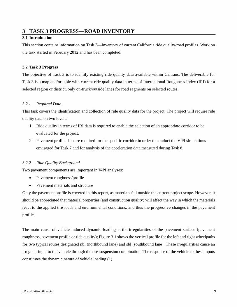
roughness, pavement profile or ride quality); Figure 3.1 shows the vertical profile for the left and right wheelpaths
for two typical routes designated nbl (northbound lane) and sbl (southbound lane). These irregularities cause an
irregular input to the vehicle through the tire-suspension combination. The response of the vehicle to these inputs
constitutes the dynamic nature of vehicle loading (1).
10 UCPRC-RR-2012-06
Figure 3.1: Example of four typical road profiles.
Pavement roughness is defined as the variation in surface elevation that induces vibrations in traversing
vehicles (2), or as “the deviations of a surface from a true planar surface with characteristic dimensions that affect
vehicle dynamics, ride quality, dynamic pavement loads, and drainage, for example, longitudinal profile,
transverse profile and cross slope” (3).
Pavement roughness is typically divided into roughness, macrotexture, and microtexture. The dividing lines
between them are based on functional considerations such as traffic safety and ride quality. Roughness is the
largest scale, with characteristic wavelengths of 0.32–328 ft (0.1–100 m) and amplitudes of 0.04–3.94 in.
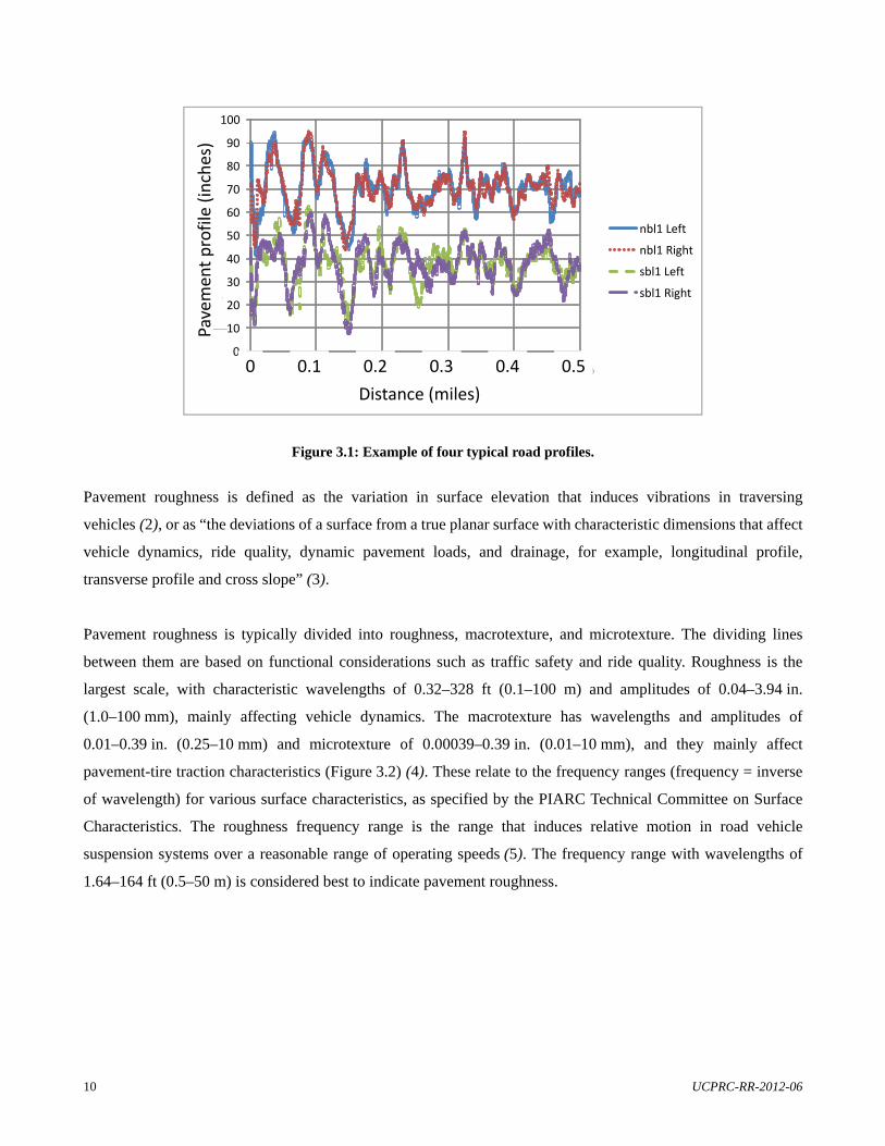
(1.0–100 mm), mainly affecting vehicle dynamics. The macrotexture has wavelengths and amplitudes of
0.01–0.39 in. (0.25–10 mm) and microtexture of 0.00039–0.39 in. (0.01–10 mm), and they mainly affect
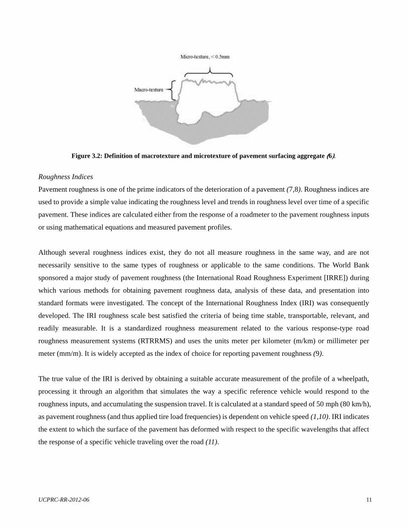
pavement-tire traction characteristics (Figure 3.2) (4). These relate to the frequency ranges (frequency = inverse
of wavelength) for various surface characteristics, as specified by the PIARC Technical Committee on Surface
Characteristics. The roughness frequency range is the range that induces relative motion in road vehicle
suspension systems over a reasonable range of operating speeds (5). The frequency range with wavelengths of
1.64–164 ft (0.5–50 m) is considered best to indicate pavement roughness.
0
10
20
30
40
50
60
70
80
90
100
0 200 400 600 800 1000
Pavement profile [mm]
Distance [m]
nbl1 Left nbl1 Right
sbl1 Left
sbl1 Right
Distance (miles)
Pavemen
t profile (inches)
0 0.1 0.2 0.3 0.4 0.5
Pavement profile [inch]
UCPRC-RR-2012-06 11
Figure 3.2: Definition of macrotexture and microtexture of pavement surfacing aggregate (6).
Roughness Indices
Pavement roughness is one of the prime indicators of the deterioration of a pavement (7,8). Roughness indices are
used to provide a simple value indicating the roughness level and trends in roughness level over time of a specific
pavement. These indices are calculated either from the response of a roadmeter to the pavement roughness inputs
or using mathematical equations and measured pavement profiles.
Although several roughness indices exist, they do not all measure roughness in the same way, and are not
necessarily sensitive to the same types of roughness or applicable to the same conditions. The World Bank
sponsored a major study of pavement roughness (the International Road Roughness Experiment [IRRE]) during
which various methods for obtaining pavement roughness data, analysis of these data, and presentation into
standard formats were investigated. The concept of the International Roughness Index (IRI) was consequently
developed. The IRI roughness scale best satisfied the criteria of being time stable, transportable, relevant, and
readily measurable. It is a standardized roughness measurement related to the various response-type road
roughness measurement systems (RTRRMS) and uses the units meter per kilometer (m/km) or millimeter per
meter (mm/m). It is widely accepted as the index of choice for reporting pavement roughness (9).
The true value of the IRI is derived by obtaining a suitable accurate measurement of the profile of a wheelpath,
processing it through an algorithm that simulates the way a specific reference vehicle would respond to the
roughness inputs, and accumulating the suspension travel. It is calculated at a standard speed of 50 mph (80 km/h),
as pavement roughness (and thus applied tire load frequencies) is dependent on vehicle speed (1,10). IRI indicates
the extent to which the surface of the pavement has deformed with respect to the specific wavelengths that affect
the response of a specific vehicle traveling over the road (11).
12 UCPRC-RR-2012-06
The Half-car Roughness Index (HRI) is based on the same equations and assumptions as the IRI, but the average
of the two wheelpaths is used in the calculation of the statistic. HRI is always less than or equal to the IRI
calculation. IRI indicates vehicle response at the tires, while HRI indicates vehicle response at the center of the
vehicle. The Median Roughness Index (MRI) is defined as the average of the IRI for the left and right wheelpaths.
The IRI of two pavements may be similar even though their roughness differs. This is possible if one pavement has
more pronounced longer wavelengths and the other more pronounced shorter wavelengths, and both these bands
fall into the IRI wavelength band (11).
IRI is particularly sensitive to wavelength bands related to shorter wavelengths (associated with axle resonance),
and longer wavelengths linked with body bounce. These wavelengths cause dynamic load variations that reduce
the road-holding ability of tires and contribute to road damage caused by commercial vehicles. The IRI is most
sensitive to slope sinusoids with wavelengths of 50 and 7.5 ft (15.4 and 2.3 m), with a gain of 1.5 and 1.65,
respectively. The gain (ratio of output amplitude to input amplitude) decreases to 0.5 for wavelengths of 100 and
4.3 ft (30.3 and 1.3 m) (11). The IRI scale ignores wavelengths outside the 4.3–100 ft (1.3–30 m) wavelength
band since these do not contribute to the roughness experienced by road-using vehicles at speeds near 50 mph
(80 km/h) (approximately 17–1.35 Hz) (2). The vehicle speed affects the perception of roughness frequency, with
higher speeds causing perceived higher frequencies as unevenness on the pavement is experienced at shorter
intervals in the vehicle.
The IRI is not related to all vehicle response variables. It is most appropriate when a roughness measure is desired
that relates to overall vehicle operating cost, overall ride quality, and overall surface condition (12). It is intended
to reflect the pavement roughness attributes that affect the ride quality of passenger vehicles and was not intended
to describe the pavement roughness characteristics affecting heavy trucks, as is needed in this report.
The IRI does not show sensitivity to excitation frequencies as observed under heavy vehicle traffic (IRI sensitivity
is at 1.5 and 11 Hz, while heavy vehicle sensitivity is at 3.5 and 12 Hz) (13). Because of these different
wavelengths affecting different vehicles, IRI is a poorer measure of ride quality for truck drivers than for car
occupants, and this is partly why this study’s analyses measured surface profile. Trucks may be more sensitive to
longer wavelengths, inducing pitch and roll response modes (5,11).
Response Modes
A vehicle traveling on a pavement has two response modes: the body bounce at frequencies typically around
1–4 Hz, and the axle hop at frequencies around 10–18 Hz (14). Vehicle response to the pavement profile can be

UCPRC-RR-2012-06 13
modeled in the frequency domain as a response function. The vehicle response characteristics amplify profile
frequencies around the natural frequencies of the response modes and attenuate profile frequencies well removed
from those of the response modes. Mathematically, the vehicle frequency response function acts as a multiplier to
the input road profile power spectral density (PSD) to give the PSD of the vehicle response (PSD measures the
frequency content of a stochastic process to assist in identifying periodicity). For frequency characterization of
road profiles and frequency domain analysis of vehicle responses to the profile, the road profile can be
characterized as a PSD. The PSD shows the variance in road profile elevation (or slope) as related to spatial
frequency (measure of how often sinusoidal components of the pavement repeat per unit of distance) (5).
Dynamic load profiles for all heavy vehicles are characterized by two distinct frequencies. Body bounce
(1.5–4 Hz) generally dominates the dynamic loading; it is mainly caused by the response of the vehicle’s sprung
mass (mass of body carried by suspension system of the vehicle) to the pavement roughness. Axle hop (8–15 Hz)
becomes more significant at higher vehicle speeds and greater pavement roughness; it is mainly caused by the
reaction of the unsprung mass (mass of tires axles and suspension system) to pavement roughness. The main cause
for the dominating effect of the body bounce may lie in the load ratio of approximately 10:1 between the sprung
mass and the unsprung mass (1).
Power Spectral Density
The PSD of pavement profiles is categorized into eight classes (A to H) according to the ISO 8608 procedure (15).
An example of three pavement profiles—with relatively smooth, average, and rough ride qualities—are shown in
Table 3.1 and Figure 3.3 to illustrate the different types of ride quality indices and related PSD classes. The
displacement power spectral density (DPSD; PSD of vertical profile) plot shows the DPSD versus spatial
frequency. Dominant peaks on this graph would indicate dominant spatial frequencies in the pavement profile data.
As relatively few such peaks occur in the data shown, no specific cause (i.e., construction faults) is expected to be
the cause of the specific roughness on the pavements indicated.
The spatial frequencies occurring at body bounce (approximately 3 Hz) and axle hop (approximately 15 Hz) at the
three speeds selected for the analyses in this report are also shown in Figure 3.3. All the lower frequencies (body
bounce) occur at positions where the DPSD indicates a marked difference between the three pavement sections.
However, the higher frequencies (axle hop) occur at DPSD values where less difference exists between the DPSD
values. This is partly caused by the dominance of higher frequencies in the DPSD analysis. As the body bounce
mode of moving dynamic loading (MDL) is the more dominant factor in MDL, due to its higher magnitude, this is
less of a concern in the various analyses.

14 UCPRC-RR-2012-06
Ride Quality Analyses
The standard software used for analysis of ride quality properties of pavement profiles is ProValTM (16). ProVal
was developed by the Federal Highway Administration, and is freely available from an FHWA website
(www.roadprofile.com). All ride quality analyses in this report have been conducted using ProVal.
Table 3.1: ISO (15) Classification and IRI and HRI Values for Three Typical Pavement Sections
Parameter Pavement Identification and Data
Smooth (S) Average (A) Rough (R) ISO classification A B/C C/D IRI (mm/m) L;R* (in./mi)
1.5; 1.5 [96; 96]
3.9; 4.4
[250; 282]
7.8; 5.5
[500; 352]96; 96 HRI (mm/m) (in./mi)
1.2 [77]
3.5
[198]
5.3
[340] *Left and right wheelpaths
Figure 3.3: Displacement power spectral densities (DPSDs) on ISO classification for three different pavements.
1.00E-08
1.00E-07
1.00E-06
1.00E-05
1.00E-04
1.00E-03
1.00E-02
1.00E-01
1.00E+00
0.01 0.1 1 10
Dis
pla
cem
ent
po
wer
sp
ect
ral
de
nsity
[m
^3]
Spatial Frequency [cycles/m]
Rough
A
B
C
E
F
G
H
D
40 km/h80 km/h
Average
Smooth
120 km/h
ISO (1995) classification
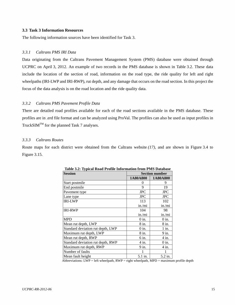
UCPRC-RR-2012-06 15
3.3 Task 3 Information Resources
The following information sources have been identified for Task 3.
3.3.1 Caltrans PMS IRI Data
Data originating from the Caltrans Pavement Management System (PMS) database were obtained through
UCPRC on April 3, 2012. An example of two records in the PMS database is shown in Table 3.2. These data
include the location of the section of road, information on the road type, the ride quality for left and right
wheelpaths (IRI-LWP and IRI-RWP), rut depth, and any damage that occurs on the road section. In this project the
focus of the data analysis is on the road location and the ride quality data.
3.3.2 Caltrans PMS Pavement Profile Data
There are detailed road profiles available for each of the road sections available in the PMS database. These
profiles are in .erd file format and can be analyzed using ProVal. The profiles can also be used as input profiles in
TruckSIMTM for the planned Task 7 analyses.
3.3.3 Caltrans Routes
Route maps for each district were obtained from the Caltrans website (17), and are shown in Figure 3.4 to
Figure 3.15.
Table 3.2: Typical Road Profile Information from PMS Database Session Section number
1A80A800 1A80A800 Start postmile 0 9 End postmile 9 19 Pavement type JPC JPC Lane type JPC JPC IRI-LWP 113
in./mi 102
in./mi IRI-RWP 104
in./mi 98
in./mi MPD 0 in. 0 in. Mean rut depth, LWP 8 in. 8 in. Standard deviation rut depth, LWP 0 in. 1 in. Maximum rut depth, LWP 8 in. 9 in. Mean rut depth, RWP 6 in. 4 in. Standard deviation rut depth, RWP 4 in. 0 in. Maximum rut depth, RWP 9 in. 4 in. Number of faults 1 1 Mean fault height 5.1 in. 5.2 in.
Abbreviations: LWP = left wheelpath, RWP = right wheelpath, MPD = maximum profile depth
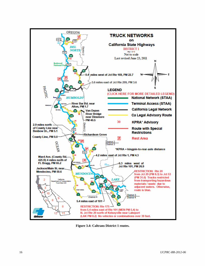
16 UCPRC-RR-2012-06
Figure 3.4: Caltrans District 1 routes.
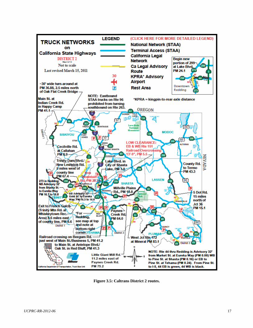
UCPRC-RR-2012-06 17
Figure 3.5: Caltrans District 2 routes.

18 UCPRC-RR-2012-06
Figure 3.6: Caltrans District 3 routes.

UCPRC-RR-2012-06 19
Figure 3.7: Caltrans District 4 routes.

20 UCPRC-RR-2012-06
Figure 3.8: Caltrans District 5 routes.

UCPRC-RR-2012-06 21
Figure 3.9: Caltrans District 6 routes.

22 UCPRC-RR-2012-06
Figure 3.10: Caltrans District 7 routes.
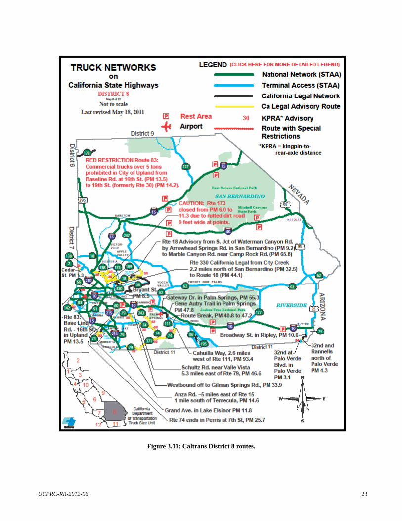
UCPRC-RR-2012-06 23
Figure 3.11: Caltrans District 8 routes.

24 UCPRC-RR-2012-06
Figure 3.12: Caltrans District 9 routes.
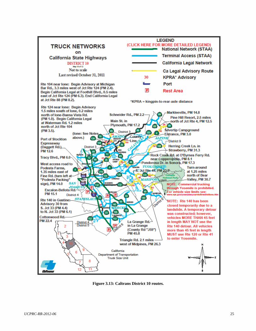
UCPRC-RR-2012-06 25
Figure 3.13: Caltrans District 10 routes.

26 UCPRC-RR-2012-06
Figure 3.14: Caltrans District 11 routes.
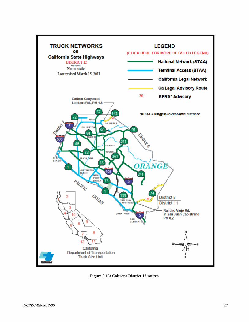
UCPRC-RR-2012-06 27
Figure 3.15: Caltrans District 12 routes.

28 UCPRC-RR-2012-06
3.4 Task 3 Analysis
The summary of the number of sections as well as miles of sections for which ride quality data exist in the current
PMS database is provided in Table 3.3 and Table 3.4. It provides an information breakdown for the various
districts (Table 3.3) and counties (Table 3.4). This represents approximately 67 percent of all the sections in
Caltrans. It is anticipated that all the sections will be available on the PMS database by July 2012.
Table 3.3: Number of Sections and Lane-Miles of Sections for Which Data Ride Quality Exist
in the Current PMS Database, by District
District
Number of sections
Lane-miles of sections
1 358 4,102.8 2 342 4,399.9 3 429 4,309.2 4 903 6,674.2 5 358 3,281.5 6 473 5,900.1 7 703 6,055.9 8 517 6,317.9 9 132 1,894.2 10 299 3,381.3 11 357 3,543.0 12 200 1,074.0 Total 50,934.0
Analysis of the data in Table 3.3 and Table 3.4 show the following:
Districts 4, 7, and 8 have the highest number of lane-miles of road with ride quality data in the current
PMS database.
Districts 9 and 12 have the lowest number of lane-miles of road with ride quality data in the current PMS
database.
LA (Los Angeles) county has the highest number of lane-miles of road with ride quality data in the current
MS database.
ALP (Alpine) county has the lowest number of lane-miles of road with ride quality data in the current
PMS database.
There are a total of 8,100 lane-miles of road in the San Joaquin Valley counties for which ride quality data
exists.
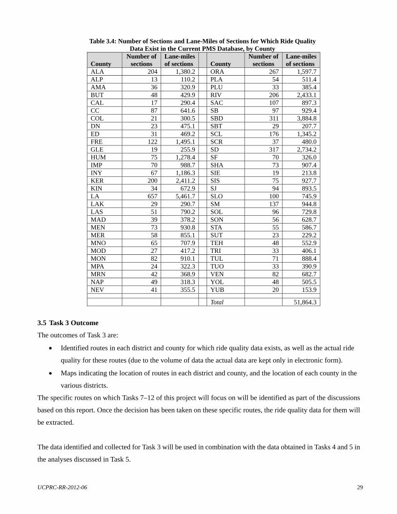
UCPRC-RR-2012-06 29
Table 3.4: Number of Sections and Lane-Miles of Sections for Which Ride Quality Data Exist in the Current PMS Database, by County
County Number of
sections Lane-miles of sections
County
Number of sections
Lane-miles of sections
ALA 204 1,380.2 ORA 267 1,597.7 ALP 13 110.2 PLA 54 511.4 AMA 36 320.9 PLU 33 385.4 BUT 48 429.9 RIV 206 2,433.1 CAL 17 290.4 SAC 107 897.3 CC 87 641.6 SB 97 929.4 COL 21 300.5 SBD 311 3,884.8 DN 23 475.1 SBT 29 207.7 ED 31 469.2 SCL 176 1,345.2 FRE 122 1,495.1 SCR 37 480.0 GLE 19 255.9 SD 317 2,734.2 HUM 75 1,278.4 SF 70 326.0 IMP 70 988.7 SHA 73 907.4 INY 67 1,186.3 SIE 19 213.8 KER 200 2,411.2 SIS 75 927.7 KIN 34 672.9 SJ 94 893.5 LA 657 5,461.7 SLO 100 745.9 LAK 29 290.7 SM 137 944.8 LAS 51 790.2 SOL 96 729.8 MAD 39 378.2 SON 56 628.7 MEN 73 930.8 STA 55 586.7 MER 58 855.1 SUT 23 229.2 MNO 65 707.9 TEH 48 552.9 MOD 27 417.2 TRI 33 406.1 MON 82 910.1 TUL 71 888.4 MPA 24 322.3 TUO 33 390.9 MRN 42 368.9 VEN 82 682.7 NAP 49 318.3 YOL 48 505.5 NEV 41 355.5 YUB 20 153.9
Total 51,864.3
3.5 Task 3 Outcome
The outcomes of Task 3 are:
Identified routes in each district and county for which ride quality data exists, as well as the actual ride
quality for these routes (due to the volume of data the actual data are kept only in electronic form).
Maps indicating the location of routes in each district and county, and the location of each county in the
various districts.
The specific routes on which Tasks 7–12 of this project will focus on will be identified as part of the discussions
based on this report. Once the decision has been taken on these specific routes, the ride quality data for them will
be extracted.
The data identified and collected for Task 3 will be used in combination with the data obtained in Tasks 4 and 5 in
the analyses discussed in Task 5.

30 UCPRC-RR-2012-06
UCPRC-RR-2012-06 31
4 TASK 4 PROGRESS—VEHICLE INVENTORY 4.1 Introduction
This section contains information on Task 4 – Inventory of current California vehicle population. Work on the task
started in February 2012 and has been completed.
4.2 Task 4 Progress
The objective of Task 4 is to identify existing vehicle population data available within Caltrans. The deliverable
for Task 4 is a table of current vehicle population per standard FHWA vehicle classifications for Caltrans.
4.3 Task 4 Information Sources
4.3.1 FHWA Vehicle Classifications
The FHWA developed the 13-vehicle class system for most federal vehicle classification count reporting
(Table 4.1) (18). Although all states currently use this classification scheme, most states separate one or more of
the FHWA categories into additional classifications to track vehicles of specific interest to them. These categories
are then aggregated when reporting to the FHWA. Fine-tuning the classification algorithm is needed because the
visual basis of the FHWA 13 categories does not translate to an exact set of axle spacings. When the FHWA 13
categories cannot be used it is recommended that the classes be either a subset of the FHWA classes or a clean
disaggregation of the FHWA classes.
4.3.2 California Truck Definitions and Information
Truck definitions for California Department of Transportation STAA routes are shown in Figure 4.1 and
Figure 4.2. The definitions used in the figures Figure 4.1are defined as follows (17):
STAA: The federal Surface Transportation Assistance Act of 1982
KPRA: kingpin-to-rear-axle distance
Double: A truck tractor that tows a semitrailer and trailer
STAA Truck: A truck tractor-semitrailer (or double) that conforms to the STAA requirements
California Legal Truck: A truck tractor-semitrailer (or double) that can travel on virtually any route in
California
National Network (NN): Primarily the interstates, also called the National System of Interstate and
Defense Highways
Terminal Access (TA) routes: State or local routes that have been granted access to STAA trucks
Service Access routes: Roads that allow STAA truck access for fuel, food, lodging, and repair within one
road mile of a signed exit from the National Network

32 UCPRC-RR-2012-06
STAA Network: The routes that allow STAA trucks, which include the National Network, Terminal
Access routes and Service Access routes
CVC: California Vehicle Code
Table 4.1: FHWA Vehicle Classes with Definitions (18) Class Description Definitions 1 Motorcycles (Optional) All two or three wheeled motorized vehicles. Typical vehicles in this category
have saddle type seats and are steered by handlebars rather than steering wheels. This category includes motorcycles, motor scooters, mopeds, motor powered bicycles, and three wheel motorcycles. This vehicle type may be reported at the option of the State.
2 Passenger Cars All sedans, coupes, and station wagons manufactured primarily for the purpose of carrying passengers and including those passenger cars pulling recreational or other light trailers.
3 Other Two Axle, Four Tire, Single Unit Vehicles
All two axle, four tire vehicles, other than passenger cars. Included in this classification are pickups, panels, vans, and other vehicles such as campers, motor homes, ambulances, hearses, carryalls, and minibuses. Other two axle, four tire, single unit vehicles pulling recreational or other light trailers are included in this classification. Because automatic vehicle classifiers have difficulty distinguishing class 3 from class 2, these two classes may be combined into class 2.
4 Buses All vehicles manufactured as traditional passenger carrying buses with two axles and six tires or three or more axles. This category includes only traditional buses (including school buses) functioning as passenger carrying vehicles. Modified buses should be considered to be a truck and should be appropriately classified.
5 Two Axle, Six Tire, Single Unit Trucks
All vehicles on a single frame including trucks, camping and recreational vehicles, motor homes, etc., with two axles and dual rear wheels.
6 Three Axle Single Unit Trucks All vehicles on a single frame including trucks, camping and recreational vehicles, motor homes, etc., with three axles.
7 Four or More Axle Single Unit Trucks
All trucks on a single frame with four or more axles.
8 Four or Fewer Axle Single Trailer Trucks
All vehicles with four or fewer axles consisting of two units, one of which is a tractor or straight truck power unit.
9 Five Axle Single Trailer Trucks
All five axle vehicles consisting of two units, one of which is a tractor or straight truck power unit.
10 Six or More Axle Single Trailer Trucks
All vehicles with six or more axles consisting of two units, one of which is a tractor or straight truck power unit.
11 Five or fewer Axle Multi Trailer Trucks
All vehicles with five or fewer axles consisting of three or more units, one of which is a tractor or straight truck power unit.
12 Six Axle Multi Trailer Trucks All six axle vehicles consisting of three or more units, one of which is a tractor or straight truck power unit.
13 Seven or More Axle Multi Trailer Trucks
All vehicles with seven or more axles consisting of three or more units, one of which is a tractor or straight truck power unit.
Note: In reporting information on trucks the following criteria should be used: Truck tractor units traveling without a trailer will be considered single-unit trucks. A truck tractor unit pulling other such units in a “saddle mount” configuration will be considered one single-unit truck and will be
defined only by the axles on the pulling unit. Vehicles are defined by the number of axles in contact with the road. Therefore, “floating” axles are counted only when in the
down position. The term “trailer” includes both semi- and full trailers.

UCPRC-RR-2012-06 33
Figure 4.1: California Truck Map legend for STAA routes (17).
Figure 4.2: California Truck Map legend for California Legal routes (17).
The FHWA classes that the California truck types aggregate to are as follows:
STAA 48 FT—Type 9 (3S2 Split)
STAA 53 FT—Type 9 (3S2)
STAA Double—Type 12 (3S1-2)
CA Legal—Type 9 (3S2)
CA Legal Double—Type 11 (2S1-2)
Typical axle distances for trucks operated in California are provided in Table 4.2 (17). These truck types have been
identified as being the most common for transporting goods in California.

34 UCPRC-RR-2012-06
Table 4.2: Most Common Truck Types in California Used for Transporting Goods Distance Between Axles (ft.)/[m] CA truck type nomenclature Axle 1 to 2 Axle 2 to 3 Axle 3 to 4 Axle 4 to 5 Axle 5 to 6 STAA 48 feet (STAA Truck Tractor-Semitrailer)—FHWA Class 9
6–26 [1.8–7.9]
3–5.99 [0.9–1.8]
6–46 [0.8–14.0]
3–10.99 [0.9–3.4]
STAA 53 feet (STAA Truck Tractor-Semitrailer)— FHWA Class 9
6–26 [1.8–7.9]
3–5.99 [0.9–1.8]
6–46 [1.8–14.0]
3–10.99 [0.9–3.4]
STAA Double (STAA Truck Tractor-Semitrailer-Trailer [Doubles])—FHWA Class 12
6–26 [1.8–7.9]
3–5.99 [0.9–1.8]
11–26 [3.4–7.9]
6–24 [1.8–7.3]
11–26 [3.4–7.9]
CA Legal Double (California Legal Truck Tractor-Semitrailer-Trailer [Doubles])— FHWA Class 9
6–26 [1.8–7.9]
11–26 [3.4–7.9]
6–20 [1.8–6.1]
11–26 [3.4–7.9]
4.3.3 Commodity Flow Survey
The Commodity Flow Survey report provides statistics of national and state-level data on domestic freight
shipments by American establishments in mining, manufacturing, wholesale, auxiliaries, and selected retail
industries. Data are provided on the types, origins, values, weights, modes of transport, distance shipped, and
ton-miles of commodities shipped. It is a shipper-based survey that is conducted every five years as part of the
Economic Census (19). Various types of data relevant to this study were obtained from this report. No specific
information for commodity flows originating outside California and transported into California (destination
California) could be identified in this pilot study.
Truck Count Data
An example of the 2010 truck count data is shown in Table 4.3, with analyzed data relevant to California shown in
Table 4.4 and Figure 4.3 to Figure 4.5.
Analysis of the data in Figure 4.3 to Figure 4.5 indicates that the four most highly populated districts carry the
highest traffic loads (in terms of average annual daily traffic [AADT]) (Figure 4.3), while the highest percentage
trucks (Figure 4.4) are located in the districts where major linkages with adjacent states or countries exist (i.e.,
Districts 2, 8, and 11) or where major interstate truck movements occur (Districts 6 and 7). District 6 forms part of
the San Joaquin Valley (refer to discussions in Sections 5 and 6).
A similar picture emerges from Figure 4.5, with the most highly populated metropolitan counties showing the
highest traffic volumes (i.e., Los Angeles, Orange, and Ventura) while counties with major interstate truck routes
or cross-border truck traffic showed higher percentage trucks on the routes (i.e., Kern, Madera, Modesto, and
Trinity).

UCPRC-RR-2012-06 35
Table 4.3: 2010 Truck Count Data Example (19) Route District County Postmile AADT
Total Total
Trucks Total Truck
Percent
2 Axle Volume
2 Axle Percent
3 Axle Volume
3 Axle Percent
4 Axle Volume
4 Axle Percent
5 Axle Volume
5 Axle Percent
Year Verified/ Estimate
1 12 ORA 0.129 37,000 2,301 6.22 781 33.93 1,089 47.32 308 13.39 123 5.36 03E 1 12 ORA 0.78 39,000 1,899 4.87 644 33.93 899 47.32 254 13.39 102 5.36 03E 1 12 ORA 9.418 40,000 696 1.74 272 39.08 320 45.98 64 9.2 40 5.75 03E
Table 4.4: Summarized Analysis of Truck Count Data per District (19) District AADT Total Total Trucks Total
Truck Percent
2 Axle/Class 5 3 Axle/Class 6 4 Axle/Classes 7 and 8 5 Axle/Classes 9 and 11 Volume Percent Volume Percent Volume Percent Volume Percent
1 1,135,860 101,876 9 46,237 45 14,475 14 5,603 5 35,207 35 2 3,662,370 540,168 15 52,913 10 33,515 6 13,907 3 416,907 77 3 12,481,183 980,516 8 334,299 34 93,000 9 45,644 5 504,006 51 4 43,707,890 1,925,535 4 850,496 44 222,646 12 72,584 4 850,374 44 5 6,270,340 478,600 8 201,503 42 46,750 10 21,406 4 195,688 41 6 8,250,955 1,417,304 17 423,796 30 94,751 7 52,977 4 816,238 58 7 56,002,040 3,283,835 6 1,301,599 40 360,991 11 125,496 4 1,428,555 44 8 21,450,950 2,351,222 11 819,266 35 182,365 8 78,184 3 1,271,394 54 9 201,825 18,334 9 5,886 32 1,778 10 917 5 9,752 53 10 6,412,135 944,602 15 194,754 21 87,701 9 30,713 3 619,819 66 11 17,715,618 940,633 5 498,081 53 95,452 10 36,021 4 304,845 32 12 19,297,800 1,057,294 5 526,137 50 102,220 10 49,109 5 342,897 32 Total 196,588,966 14,039,919 7 5,254,967 37 1,335,644 10 532,561 4 6,795,682 48
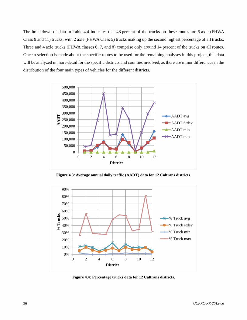
36 UCPRC-RR-2012-06
The breakdown of data in Table 4.4 indicates that 48 percent of the trucks on these routes are 5 axle (FHWA
Class 9 and 11) trucks, with 2 axle (FHWA Class 5) trucks making up the second highest percentage of all trucks.
Three and 4 axle trucks (FHWA classes 6, 7, and 8) comprise only around 14 percent of the trucks on all routes.
Once a selection is made about the specific routes to be used for the remaining analyses in this project, this data
will be analyzed in more detail for the specific districts and counties involved, as there are minor differences in the
distribution of the four main types of vehicles for the different districts.
Figure 4.3: Average annual daily traffic (AADT) data for 12 Caltrans districts.
Figure 4.4: Percentage trucks data for 12 Caltrans districts.
0
50,000
100,000
150,000
200,000
250,000
300,000
350,000
400,000
450,000
500,000
0 2 4 6 8 10 12
AA
DT
District
AADT avg
AADT Stdev
AADT min
AADT max
0%
10%
20%
30%
40%
50%
60%
70%
80%
90%
0 2 4 6 8 10 12
% T
ruck
s
District
% Truck avg
% Truck stdev
% Truck min
% Truck max

UCPRC-RR-2012-06 37
Figure 4.5: AADT and percentage trucks data for Caltrans counties (=AADT; × = % Trucks).
4.3.4 Truck Traffic Analysis Using WIM Data in California
Lu et al. (20) analyzed weigh-in-motion (WIM) data for the decade 1991–2001. In lieu of a more recent updated
version of this report, the information originating from this report was used to obtain an indication of the truck
traffic trends in California. A preliminary comparison between these data and the latest data on the WIM database
(not analyzed in the same manner) indicates that similar trends exist in the latest data. Data from the latest WIM
measurements will be verified when a specific corridor has been selected for this pilot study. Figure 4.6 shows the
location of WIM stations in California. Table 4.5 shows the basic information for each WIM station in California.
Table 4.5: Summary of Basic Information for Each WIM Station in California (20)
Station Number
Location Information
WIM System
Lane Configuration
Name District County Route Postmile Number of Lanes Direction
1 Lodi 10 San Joaquin 5 43.7 DAW 200 4 N2N1S1S2 2 Redding 2 Shasta 5 R24.9 DAW 200
(7/99) 4 S2S1N1N2
IRD (7/99–present)
4 N2N1S1S2
3 Antelope 3 Sacramento 80 15 DAW 200 (8/95)
4 W4W3W2W1
Antelope (EB) After 95
IRD (8/95–present)
4 E4E3E2E1
4 Antelope (WB) After 98
3 Sacramento 80 17.2 IRD 4 W4W3W2W1
0%
5%
10%
15%
20%
25%
0
17,500
35,000
52,500
70,000
87,500
105,000
122,500
140,000
157,500
175,000
AL
AA
LP
AM
AB
UT
CA
LC
CC
OL
DN
ED
FR
EG
LE
HU
MIM
PIN
YK
ER
KIN LA
LA
KL
AS
MA
DM
EN
ME
NM
ER
MN
OM
OD
MO
NM
PAM
RN
NA
PN
EV
OR
APL
APL
UR
IVSA
CSB
SBD
SB
TS
CL
SCR
SD SFSH
ASI
ESI
S SJSL
OSM SO
LSO
NST
ASU
TT
EH
TR
IT
UL
TU
OV
EN
YO
LY
UB
Ave
rage
% T
ruck
s
Ave
rage
AA
DT
County

38 UCPRC-RR-2012-06
Conclusions from the WIM analysis (20) that are of importance to this report are as follows:
Across all truck types operating in California (legal load limit for single axle loads is 20 kip [89 kN], legal
limit for tandem axle loads is 34 kip [151 kN]):
o A small portion of the axle loads are over the legal limit.
o Nearly all steering axle loads are less than 20 kip (90 kN).
o Nearly all single axle loads are less than 24.7 kip (110 kN).
o Nearly all tandem axle loads are less than 47.2 kip (210 kN).
o Nearly all tridem axle loads are less than 58.4 kip (260 kN).
All four axle types had a bimodal pattern of load spectra (distribution of loads). For tandem axles, the
bimodal pattern is due to the empty and full load status of Truck Type 9 (the predominant truck type,
consisting of a tractor with a tandem axle and a single semitrailer with a tandem axle [3S2]). For the other
three axle types, the bimodal pattern is caused by the different load levels associated with the various
truck types.
Axle load spectra are heavier (heavier axle loads) at night than in the daytime. Two possible reasons for
this are (1) it is more efficient to carry heavier loads when car traffic is lighter and (2) heavier, potentially
overloaded trucks operate more at night when more Highway Patrol load enforcement stations are closed.
Axle load spectra and truck type distribution show very little seasonal variation. This contradicts the
assumption that truck loads are significantly influenced by agricultural hauling during the harvest season.
Axle load spectra are much higher (heavier axle loads) in the Central Valley than in the Bay Area and
Southern California, particularly for tandem axles. Axle load spectra are similar between the Bay Area
and Southern California.
The predominant truck types across the state are Truck Type 9, accounting for 49 percent of all trucks, and
Truck Type 5 (2-axle truck with dual tires at the back [2D]), accounting for 23 percent of all trucks. Truck
Type 11 (tractor with single axle, one semitrailer with a single axle and another trailer with single axles
[2S12]) accounted for 8 percent of all trucks, and the rest of the truck types together accounted for the
remaining 20 percent of all trucks.
Data from a set of six WIM sites selected to represent different combinations of direction, region (Bay Area,
Central Valley, and Southern California), and urban versus rural indicated that:
Steering axle load spectra were similar across all six stations.
Axle load spectra for other axle types varied considerably across the six stations.
Axle load spectra were similar for both directions.
Axle load spectra were much heavier in the outside lanes.
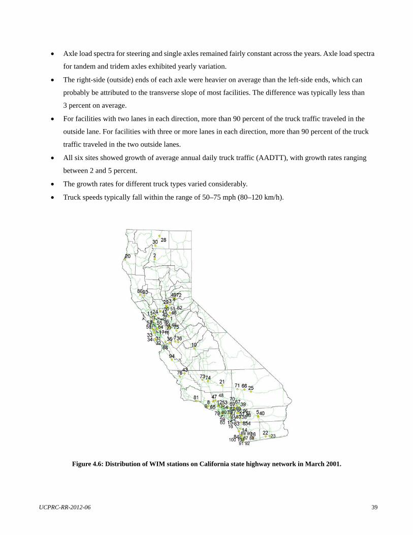
UCPRC-RR-2012-06 39
Axle load spectra for steering and single axles remained fairly constant across the years. Axle load spectra
for tandem and tridem axles exhibited yearly variation.
The right-side (outside) ends of each axle were heavier on average than the left-side ends, which can
probably be attributed to the transverse slope of most facilities. The difference was typically less than
3 percent on average.
For facilities with two lanes in each direction, more than 90 percent of the truck traffic traveled in the
outside lane. For facilities with three or more lanes in each direction, more than 90 percent of the truck
traffic traveled in the two outside lanes.
All six sites showed growth of average annual daily truck traffic (AADTT), with growth rates ranging
between 2 and 5 percent.
The growth rates for different truck types varied considerably.
Truck speeds typically fall within the range of 50–75 mph (80–120 km/h).
Figure 4.6: Distribution of WIM stations on California state highway network in March 2001.
40 UCPRC-RR-2012-06
4.3.5 Truck Route List
A truck route list was obtained from the Caltrans website (Office of Truck Services) (17). It provides information
on typical truck routes followed in California; the type of details are shown in Table 4.6. The data provide the
standard origin and destination information for each of the routes, as well as information on restrictions for the
specific routes. A summary of these restrictions is provided in Table 4.7.
4.3.6 Truck Tire and Suspension Use
In order for the analyses in Task 7 to be conducted it is important to know the type of tires and suspension used by
trucks on the various routes. Although a detailed evaluation will be conducted once a final corridor and trucks are
selected for the Task 8 measurements, a preliminary evaluation of the dominant tire and suspension types was
conducted.
No recent California-specific data could be identified on this topic, however, a 2004 report originating from Texas
focused on current truck configurations on Texas highways. As the truck population in the United States is
relatively homogeneous, the data collected and summarized in this report are used as a preliminary indication of
these dominant factors (21).
It was found, based on a sample of 623 trucks with 9,600 tires, that:
The overall average tire inflation pressure was 96.75 psi (667 kPa) with a standard deviation of
15.03 psi (103.6 kPa).
295-75R22.5 (25.7 percent), 11R24.5 (21.8 percent), 11R22.5 (17.3 percent), and 285-75R24.5
(15.4 percent) were the four most popular tire sizes found in the sampled trucks.
11R24.5 (24.1 percent) was the most popular tire size on front (steering) axles.
295-75R22.5 (26.2 percent) was the most popular nonfront tire.
Very few wide-base tires were noted.
Leaf springs were predominantly used in steering axles (98 percent).
Drive axles mostly used air suspension (72 percent).
Trailer axles used mostly leaf suspension (66 percent).
Incidentally, the most common truck class was 3-S2 (80.3 percent), which is classified as STAA (or FWHA
Class 9) trucks. These trucks were also dominant in the California surveys (Table 4.4).
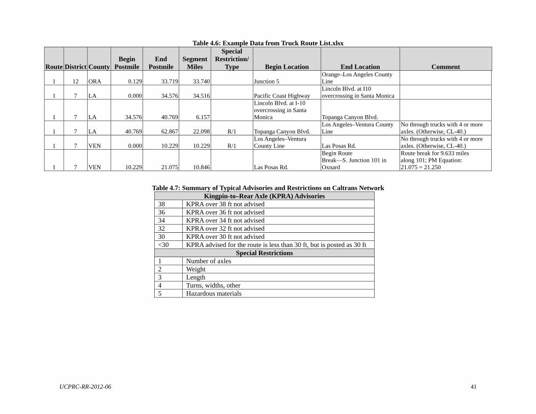
UCPRC-RR-2012-06 41
Table 4.6: Example Data from Truck Route List.xlsx
Route District County Begin
Postmile End
Postmile Segment
Miles
Special Restriction/
Type Begin Location End Location Comment
1 12 ORA 0.129 33.719 33.740
Junction 5 Orange–Los Angeles County Line
1 7 LA 0.000 34.576 34.516
Pacific Coast Highway Lincoln Blvd. at I10 overcrossing in Santa Monica
1 7 LA 34.576 40.769 6.157
Lincoln Blvd. at I-10 overcrossing in Santa Monica Topanga Canyon Blvd.
1 7 LA 40.769 62.867 22.098 R/1 Topanga Canyon Blvd. Los Angeles–Ventura County Line
No through trucks with 4 or more axles. (Otherwise, CL-40.)
1 7 VEN 0.000 10.229 10.229 R/1 Los Angeles–Ventura County Line Las Posas Rd.
No through trucks with 4 or more axles. (Otherwise, CL-40.)
1 7 VEN 10.229 21.075 10.846
Las Posas Rd.
Begin Route Break—S. Junction 101 in Oxnard
Route break for 9.633 miles along 101; PM Equation: 21.075 = 21.250
Table 4.7: Summary of Typical Advisories and Restrictions on Caltrans Network Kingpin-to–Rear Axle (KPRA) Advisories
38 KPRA over 38 ft not advised 36 KPRA over 36 ft not advised 34 KPRA over 34 ft not advised 32 KPRA over 32 ft not advised 30 KPRA over 30 ft not advised <30 KPRA advised for the route is less than 30 ft, but is posted as 30 ft
Special Restrictions 1 Number of axles 2 Weight 3 Length 4 Turns, widths, other 5 Hazardous materials
42 UCPRC-RR-2012-06
4.4 Task 4 Outcome
The objective of Task 4 is to develop an inventory of current California vehicle population. For this purpose
information was sourced from various statewide sources. The outcome of Task 4 is:
A table of current vehicle population by standard FHWA vehicle classification. These data are summarized in
Table 4.4.
The data identified and collected for Task 3 will be used in combination with the data obtained in Tasks 4–5 in the
analyses discussed in Task 5.

UCPRC-RR-2012-06 43
5 TASK 5 PROGRESS—INFORMATION REVIEW 5.1 Introduction
This section contains information on the progress with Task 5—Research/review available information resources.
Work on the task started in February 2012 and the first draft is completed. Once the inputs of the client have been
obtained on the current (first draft) version, the information will be updated and a final output prepared.
5.2 Task 5 Progress
Task 5 focuses on evaluating the data obtained from the various resources for Tasks 3–4, as well as additional
relevant information that may add to the project. Potential sources include pavement condition survey (PCS) and
new Pavement Management System (PMS) data, State of Logistics studies, rolling resistance studies (MIRIAM
project), and various California-specific studies and models (e.g., Statewide Freight Model, Heavy-Duty Truck
Model [SCAG]), as well as related U.S./California studies into V-PI and ride quality.
The deliverable of Task 5 is a detailed understanding and input to the progress report on the available data sources
and required analyses for the project, inclusive of indications of the potential links between the outputs from this
project and the inputs for the various economic and planning models. Final selection of an appropriate route
covering a range of ride qualities and speeds within the selected region/district for potential truck measurements
will be made by Caltrans after evaluation of all relevant information.
5.3 Task 5 Information Resources
The following information sources have been identified for Task 5, in addition to the sources discussed in
Sections 3 and 4.
A schematic indication of the way the various transportation models relate to each other is shown in Figure 5.1.
Each of the separate models is discussed in this section as an information source, before an analysis is conducted
using all the available information.
Figure 5.1: Schematic of how the various transportation models are being developed
Statewide Travel Demand Model
Statewide Freight Model
Statewide Integrated
Transportation, Land‐use and
Economic Model
44 UCPRC-RR-2012-06
5.3.1 California Statewide Freight Planning
The Caltrans Division of Transportation Systems Information (TSI) houses the Statewide Freight Planning group.
The California Statewide Freight Forecast (CSFF) model supports the need for a statewide, commodity-based,
policy-sensitive and freight infrastructure–based transportation model. The California Statewide Travel Demand
Model (CSTDM) and various freight models (e.g., the SCAG) existed before development of the CSFF model.
The purpose of the CSFF model is to provide a policy-sensitive model to forecast commodity flows and
commercial vehicle flows within California, addressing socioeconomic conditions, land-use policies related to
freight, environmental policies, and multimodal infrastructure investments. The model development project has a
two-year timeline and it is due for completion by June 2013. Due to the anticipated completion date for the CSFF
model, it will not affect the pilot study, but may affect the potential implementation of the findings of the pilot
study.
The CSFF has been developed in three phases. The first phase focused on development of a Freight Data
Repository that included compilation of 16 different publicly available freight data sources
http://moon.its.uci.edu/calfred/). The second phase focused on developing a conceptual framework for the
Statewide Freight Model and consisted of developing the scope, time, and cost for full construction of the freight
model. The third phase started in October 2011 and focuses on the construction of the Statewide Freight Model. It
is developed (as the other phases of the project) by UC Irvine and planned to be completed by June 2013.
5.3.2 Commodity Flow Survey
Section 4.3.3 stated that the Commodity Flow Survey report provides statistics of national and state-level data on
domestic freight shipments by American establishments in mining, manufacturing, wholesale, auxiliaries, and
selected retail industries originating in California. (Data on flow originating from others states are also available,
but this report focuses on California.) Data are provided on the types, origins, values, weights, modes of transport,
distance shipped, and ton-miles of commodities shipped. It is a shipper-based survey conducted every five years
as part of the Economic Census (19). Various types of data relevant to this study were obtained from this report. In
this section the focus is on shipment data. No specific information for commodity flows into California
(destination California) could be identified in this pilot study.
Shipment Characteristics by Mode of Transportation
Shipment characteristics by mode of transportation for freight trips originating in California is shown in Table 5.1.
It is evident that truck-based transportation dominates the freight transportation scene in the state. The data in each

UCPRC-RR-2012-06 45
of the columns are combinations of the different modes of transportation and do not necessarily add up to
100 percent in each case.
It is also noted that 82 percent of the tons shipped from California utilize only trucks and do not make use of
truck-rail or other modal combinations. This is significant, as it implies that freight is not transferred between
modes. However, freight may still be transferred between different trucks. In the notes to Table 5.1 it is clear that
this 82 percent includes for-hire and private truck combinations. Truck as a single mode also accounts for
66.7 percent of the monetary value of outgoing shipments and 72.6 percent of the total ton-miles, making this
mode by far the most impactful mode of transport in terms of physical traffic, freight flow, and economic impact.
A ton-mile is one ton of freight transported over one mile. The more ton-miles incurred by a shipment, the more
that shipment is subjected to V-PI and the higher the probability of freight damage.
It is interesting to note that the road-rail split for freight shipped from California is similar to the road-rail split for
land freight in South Africa. In 2010, 70.2 percent of the ton-miles incurred by land freight movement (i.e.,
excluding air and coastal shipping) in South Africa were by road, while 29.8 percent was by rail (22). Table 5.1
shows that 72.6 percent of the ton-miles traveled by freight shipped from California is by road, while 9.2 percent
is rail-only, and 6.7 percent uses a road-rail (intermodal) combination. These figures are not exactly comparable,
but a mention of the underlying logistics trends is worthwhile.
In South Africa, service unreliability and cost and time inefficiencies in the rail environment are commonly cited
as reasons why truck transport is preferred over rail transport, even for “rail-friendly ” freight. The current
road-rail split in South Africa is a cause of great concern from a transport vulnerability and sustainability point of
view—especially in light of recent oil-price volatility. The reasons for the road-rail split of outgoing freight in
California may very well be different from the South African situation. One reason could be a lack of capacity in
the rail western rail system. However, given that shipments leaving California are either being exported by sea (as
bulk or loaded in intermodal containers) or traveling across the vast interior of the United States, it does seem
intuitive that more freight should travel by rail. Another restriction to intermodal transportation (truck-rail
combinations) could be industry reluctance to using intermodal containers for domestic freight.
Comparing the statistics of for-hire trucks and private trucks it is observed that although more tons are carried on
private trucks, the ton-miles accrued to for-hire trucks far outweigh that of private trucks. Similarly, the average
miles per shipment are 962 for for-hire trucks and only 47 for private trucks. This suggests that for-hire trucks are
used for long-haul transportation while private fleets are mainly used for local distribution, which is intuitive.

46 UCPRC-RR-2012-06
It is important to note that Table 5.1 only lists statistics for shipments that originate in California. These shipments
could be destined for in-state locations or exported to other states or countries. The table does not account for
shipments that originate outside of California but are destined for locations inside California. Thus the statistics do
not give an overall view of all freight shipments in California.
Commodity Characteristics of Shipments
Table 5.2 classifies California shipments according to North American Industry Classification System (NAICS)
codes for all types of trucks. Table 5.2 again only focuses on shipments originating from California and thus is not
an accurate reflection of all shipments traveling in the state. The data indicate that the highest percentage of
commodities (in terms of value, tons, and ton-miles) transported by truck are manufacturing goods, wholesale
trade. and nondurable goods for the whole of California. These percentages will differ for specific counties and
districts, but this detail is not available from the source.
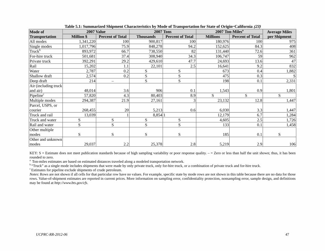
UCPRC-RR-2012-06 47
Table 5.1: Summarized Shipment Characteristics by Mode of Transportation for State of Origin—California (23) Mode of Transportation
2007 Value 2007 Tons 2007 Ton-Milesa Average Miles per Shipment Million $ Percent of Total Thousands Percent of Total Millions Percent of Total
All modes 1,341,220 100 900,817 100 180,976 100 975Single modes 1,017,796 75.9 848,278 94.2 152,625 84.3 408Truckb 893,972 66.7 738,550 82 131,440 72.6 361For-hire truck 501,681 37.4 308,940 34.3 106,747 59 962Private truck 392,291 29.2 429,610 47.7 24,693 13.6 47Rail 15,202 1.1 22,101 2.5 16,641 9.2 832Water 2,787 0.2 S S 673 0.4 1,882Shallow draft 2,574 0.2 S S 475 0.3 SDeep draft 214 – S S 198 0.1 2,331Air (including truck and air) 48,014 3.6 906 0.1 1,543 0.9 1,801Pipelinec 57,820 4.3 80,403 8.9 S S S Multiple modes 294,387 21.9 27,161 3 23,132 12.8 1,447Parcel, USPS, or courier 268,455 20 5,213 0.6 6,030 3.3 1,447Truck and rail 13,039 1 8,854 1 12,179 6.7 1,284Truck and water S S S S 4,605 2.5 1,726Rail and water S S S S 133 0.1 1,458Other multiple modes S S S S 185 0.1 S Other and unknown modes 29,037 2.2 25,378 2.8 5,219 2.9 106 KEY: S = Estimate does not meet publication standards because of high sampling variability or poor response quality. – = Zero or less than half the unit shown; thus, it has been rounded to zero. a Ton-miles estimates are based on estimated distances traveled along a modeled transportation network. b “Truck” as a single mode includes shipments that were made by only private truck, only for-hire truck, or a combination of private truck and for-hire truck. c Estimates for pipeline exclude shipments of crude petroleum. Notes: Rows are not shown if all cells for that particular row have no values. For example, specific state by mode rows are not shown in this table because there are no data for those rows. Value-of-shipment estimates are reported in current prices. More information on sampling error, confidentiality protection, nonsampling error, sample design, and definitions may be found at http://www.bts.gov/cfs.

48 UCPRC-RR-2012-06
Table 5.2:Summary of Freight Descriptions (for NAICS Industries) Transported in 2007—All TrucksNAICS Description (All Truck Types)
2007 Value 2007 Tons 2007 Ton-Miles Million $ Percent Thousands Percent Millions Percent
Apparel manufacturing 5,480 0.1 42 0.0 2 0.0 Apparel, piece goods, and notions merchant wholesalers 22,170 0.5 2,829 0.1 2,264 0.3 Beer, wine, and distilled alcoholic beverage merchant wholesalers 28,586 0.7 13,228 0.4 549 0.1 Beverage and tobacco product manufacturing 27,585 0.7 31,145 1.0 6,712 0.9 Chemical and allied products merchant wholesalers 18,984 0.5 13,518 0.4 5,794 0.8 Chemical manufacturing 55,940 1.4 40,106 1.3 27,406 3.8 Commercial equipment merchant wholesalers 47,521 1.2 4,010 0.1 1,262 0.2 Computer and electronic product manufacturing 51,951 1.3 860 0.0 641 0.1 Corporate, subsidiary, and regional managing offices 45,194 1.1 26,127 0.8 12,458 1.7 Drugs and druggists’ sundries merchant wholesalers 50,484 1.2 3,784 0.1 2,102 0.3 Electrical and electronic goods merchant wholesalers 48,376 1.2 4,347 0.1 1,676 0.2 Electrical equipment, appliance, and component manufacturing 18,342 0.4 3,086 0.1 4,622 0.6 Electronic shopping and mail-order houses 5,994 0.1 796 0.0 350 0.0 Fabricated metal product manufacturing 41,104 1.0 9,368 0.3 5,844 0.8 Farm product raw material merchant wholesalers 7,038 0.2 11,234 0.4 3,869 0.5 Food manufacturing 126,075 3.1 98,744 3.1 50,840 7.1 Fuel dealers 388 0.0 450 0.0 14 0.0 Furniture and home furnishing merchant wholesalers 13,618 0.3 4,892 0.2 2,251 0.3 Furniture and related product manufacturing 18,332 0.4 5,293 0.2 3,897 0.5 Grocery and related product merchant wholesalers 139,840 3.4 81,965 2.6 18,519 2.6 Hardware and plumbing merchant wholesalers 20,582 0.5 3,568 0.1 936 0.1 Leather and allied product manufacturing 595 0.0 147 0.0 272 0.0 Lumber and other construction materials merchant wholesalers 27,982 0.7 37,057 1.2 5,808 0.8 Machinery manufacturing 36,263 0.9 3,469 0.1 4,844 0.7 Machinery, equipment, and supplies merchant wholesalers 40,420 1.0 10,639 0.3 4,510 0.6 Manufacturing 621,991 15.2 599,374 18.9 186,600 26.2 Merchant wholesalers, durable goods 394,593 9.6 275,942 8.7 47,569 6.7 Merchant wholesalers, nondurable goods 472,374 11.5 344,614 10.9 59,567 8.4 Metal and mineral (except petroleum) merchant wholesalers 23,154 0.6 11,111 0.3 2,337 0.3 Mining (except oil and gas) 5,889 0.1 214,304 6.7 12,413 1.7 Miscellaneous durable goods merchant wholesalers 44,024 1.1 14,195 0.4 19,613 2.8 Miscellaneous manufacturing 14,472 0.4 1,276 0.0 2,044 0.3 Miscellaneous nondurable goods merchant wholesalers 36,103 0.9 37,093 1.2 6,808 1.0 Motor vehicle and parts merchant wholesalers 126,943 3.1 4,720 0.1 3,225 0.5 Newspaper, periodical, book, and directory publishers 3,805 0.1 2,406 0.1 662 0.1 Nonmetallic mineral product manufacturing 24,838 0.6 193,329 6.1 15,498 2.2

UCPRC-RR-2012-06 49
NAICS Description (All Truck Types)
2007 Value 2007 Tons 2007 Ton-Miles Million $ Percent Thousands Percent Millions Percent
Paper and paper product merchant wholesalers 20,566 0.5 10,055 0.3 1,686 0.2 Paper manufacturing 28,832 0.7 23,673 0.7 17,247 2.4 Petroleum and coal products manufacturing 25,735 0.6 128,243 4.0 6,569 0.9 Petroleum and petroleum products merchant wholesalers 143,813 3.5 169,460 5.3 7,532 1.1 Plastics and rubber products manufacturing 31,850 0.8 12,527 0.4 9,099 1.3 Primary metal manufacturing 20,823 0.5 10,908 0.3 8,327 1.2 Printing and related support activities 11,993 0.3 5,004 0.2 3,418 0.5 Textile mills 3,986 0.1 828 0.0 924 0.1 Textile product mills 4,737 0.1 704 0.0 851 0.1 Transportation equipment manufacturing 48,927 1.2 4,648 0.1 7,056 1.0 Warehousing and storage 201,827 4.9 52,599 1.7 9,873 1.4 Wholesale trade 866,966 21.2 623,157 19.6 106,672 15.0 Wood product manufacturing 14,945 0.4 24,425 0.8 10,107 1.4 Total 4,092,030 3,175,299 713,139
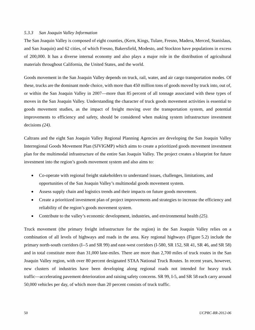
50 UCPRC-RR-2012-06
5.3.3 San Joaquin Valley Information
The San Joaquin Valley is composed of eight counties, (Kern, Kings, Tulare, Fresno, Madera, Merced, Stanislaus,
and San Joaquin) and 62 cities, of which Fresno, Bakersfield, Modesto, and Stockton have populations in excess
of 200,000. It has a diverse internal economy and also plays a major role in the distribution of agricultural
materials throughout California, the United States, and the world.
Goods movement in the San Joaquin Valley depends on truck, rail, water, and air cargo transportation modes. Of
these, trucks are the dominant mode choice, with more than 450 million tons of goods moved by truck into, out of,
or within the San Joaquin Valley in 2007—more than 85 percent of all tonnage associated with these types of
moves in the San Joaquin Valley. Understanding the character of truck goods movement activities is essential to
goods movement studies, as the impact of freight moving over the transportation system, and potential
improvements to efficiency and safety, should be considered when making system infrastructure investment
decisions (24).
Caltrans and the eight San Joaquin Valley Regional Planning Agencies are developing the San Joaquin Valley
Interregional Goods Movement Plan (SJVIGMP) which aims to create a prioritized goods movement investment
plan for the multimodal infrastructure of the entire San Joaquin Valley. The project creates a blueprint for future
investment into the region’s goods movement system and also aims to:
Co-operate with regional freight stakeholders to understand issues, challenges, limitations, and
opportunities of the San Joaquin Valley’s multimodal goods movement system.
Assess supply chain and logistics trends and their impacts on future goods movement.
Create a prioritized investment plan of project improvements and strategies to increase the efficiency and
reliability of the region’s goods movement system.
Contribute to the valley’s economic development, industries, and environmental health (25).
Truck movement (the primary freight infrastructure for the region) in the San Joaquin Valley relies on a
combination of all levels of highways and roads in the area. Key regional highways (Figure 5.2) include the
primary north-south corridors (I--5 and SR 99) and east-west corridors (I-580, SR 152, SR 41, SR 46, and SR 58)
and in total constitute more than 31,000 lane-miles. There are more than 2,700 miles of truck routes in the San
Joaquin Valley region, with over 80 percent designated STAA National Truck Routes. In recent years, however,
new clusters of industries have been developing along regional roads not intended for heavy truck
traffic—accelerating pavement deterioration and raising safety concerns. SR 99, I-5, and SR 58 each carry around
50,000 vehicles per day, of which more than 20 percent consists of truck traffic.

UCPRC-RR-2012-06 51
According to the FHWA’s Freight Analysis Framework (FAF3) routing tool, the main highway corridors used for
truck movements are I-5, SR 99, and I-580 to 205, with all these corridors carrying volumes in excess of
10 million annual tons. Truck volumes moving on key truck route corridors in the San Joaquin Valley are shown in
Table 5.3; I-5 and SR 99 carry the highest overall truck volumes (24).
Fifty-three percent of the freight moved by truck into, out of, and within the San Joaquin Valley in 2007 was
classified as internal moves, with around 23 percent shipped outbound and 24 percent shipped inbound to the San
Joaquin Valley (Figure 5.3). The internal commodity flows demonstrate the interconnectedness of the valley’s
supply chain, with products being shipped by truck within the region for further processing, consolidation, and
then distribution to other regions (24).
Farm products are the dominant commodity carried outbound from the San Joaquin Valley, comprising 33 percent
of the total outbound movements (Figure 5.4). They consist of fresh field crops (vegetables, fruit and nuts, cereal
grains, and animal feed). Stone and aggregates account for 18 percent of the total; food and tobacco products
around 10 percent; and waste and mixed freight, 6 percent and 4 percent of the total tonnage, respectively.
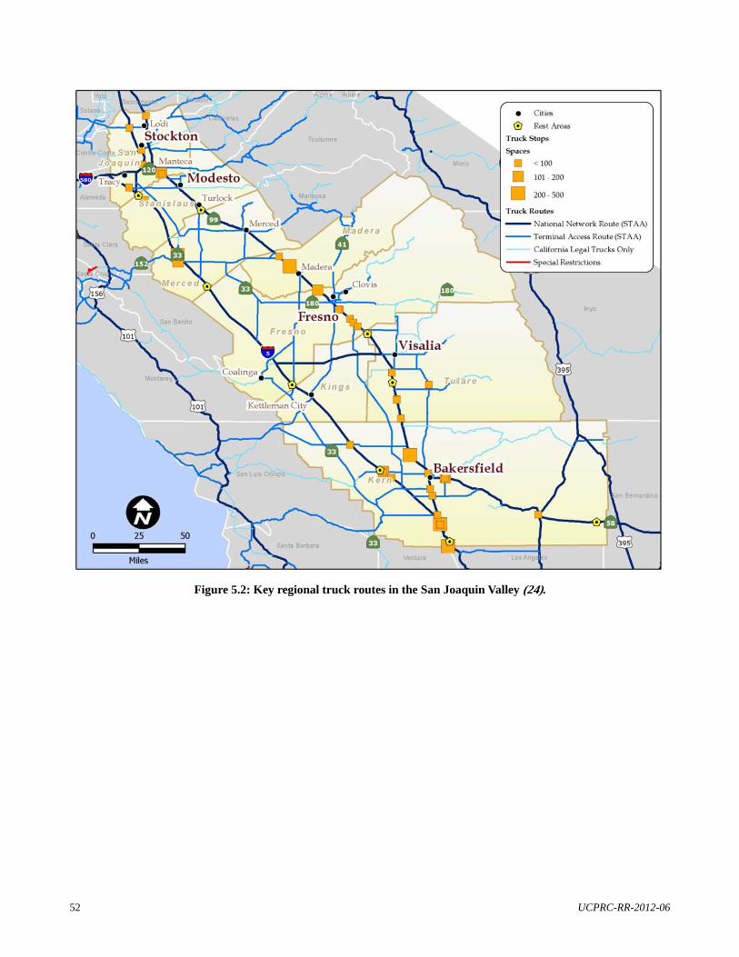
52 UCPRC-RR-2012-06
Figure 5.2: Key regional truck routes in the San Joaquin Valley (24).

UCPRC-RR-2012-06 53
Table 5.3: Major Highway Corridors and Proportion of Truck Traffic, San Joaquin Valley (24)
Facility Type Route
Number County Maximum
AADT Truck AADT
Truck Percent Facility Type
Route Number
Interstate 5 San Joaquin, Merced, Fresno, Kern 152,000 39,500 26 Interstate 5 State route 58 Kern 70,000 17,500 25 State route 58 State route 99 All San Joaquin Valley 132,000 27,700 21 State route 99 State route 119 Kern 12,500 2,600 21 State route 119 State route 46 Kern 10,500 2,000 19 State route 46 State route 190 Tulare 23,100 4,200 18 State route 190 Interstate 580 San Joaquin 32,000 5,800 18 Interstate 580 State route 33 Merced, Fresno, Kern 11,800 1,700 14 State route 33 State route 43 Fresno, Kings, Kern 18,500 2,600 14 State route 43 State route 201 Fresno 17,600 2,500 14 State route 201 State route 4 San Joaquin 89,000 11,600 13 State route 4 State route 137 Tulare 25,000 3,000 12 State route 137 Interstate 205 San Joaquin 105,000 12,600 12 Interstate 205 State route 132 San Joaquin, Stanislaus 19,200 1,900 10 State route 132 State route 145 Madera, Fresno 19,100 1,900 10 State route 145 State route 12 San Joaquin 35,000 3,200 9 State route 12 State route 65 Tulare, Kern 24,700 2,200 9 State route 65 State route 152 Merced, Madera 33,500 3,000 9 State route 152 State route 196 Kings, Tulare 61,000 5,500 9 State route 196 State route 219 Stanislaus 14,200 1,300 9 State route 219
Figure 5.3: Inbound, outbound, and internal commodity distribution, 2007 (24).
Inbound24%
Outbound23%
Internal53%
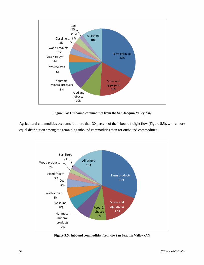
54 UCPRC-RR-2012-06
Figure 5.4: Outbound commodities from the San Joaquin Valley (24)
Agricultural commodities accounts for more than 30 percent of the inbound freight flow (Figure 5.5), with a more
equal distribution among the remaining inbound commodities than for outbound commodities.
Figure 5.5: Inbound commodities from the San Joaquin Valley (24).
Farm products
31%
Stone and
aggregates
17%Food &tobacco
8%Nonmetal
mineral
products
7%
Gasoline 6%
Waste/scrap
5%
Coal
4%
Mixed freight
3%
Wood products 2%
Fertilizers
2% All others
15%
Farm products
33%
Stone and
aggregates
18%Food and
tobacco
10%
Nonmetal
mineral products
8%
Waste/scrap
6%
Mixed freight
4%
Wood products 3%
Gasoline
3%
Coal 3%
Logs
2%
All others
10%
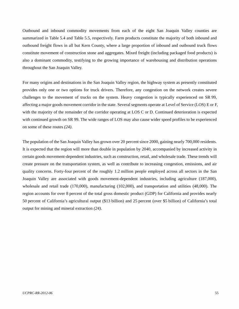
UCPRC-RR-2012-06 55
Outbound and inbound commodity movements from each of the eight San Joaquin Valley counties are
summarized in Table 5.4 and Table 5.5, respectively. Farm products constitute the majority of both inbound and
outbound freight flows in all but Kern County, where a large proportion of inbound and outbound truck flows
constitute movement of construction stone and aggregates. Mixed freight (including packaged food products) is
also a dominant commodity, testifying to the growing importance of warehousing and distribution operations
throughout the San Joaquin Valley.
For many origins and destinations in the San Joaquin Valley region, the highway system as presently constituted
provides only one or two options for truck drivers. Therefore, any congestion on the network creates severe
challenges to the movement of trucks on the system. Heavy congestion is typically experienced on SR 99,
affecting a major goods movement corridor in the state. Several segments operate at Level of Service (LOS) E or F,
with the majority of the remainder of the corridor operating at LOS C or D. Continued deterioration is expected
with continued growth on SR 99. The wide ranges of LOS may also cause wider speed profiles to be experienced
on some of these routes (24).
The population of the San Joaquin Valley has grown over 20 percent since 2000, gaining nearly 700,000 residents.
It is expected that the region will more than double in population by 2040, accompanied by increased activity in
certain goods movement-dependent industries, such as construction, retail, and wholesale trade. These trends will
create pressure on the transportation system, as well as contribute to increasing congestion, emissions, and air
quality concerns. Forty-four percent of the roughly 1.2 million people employed across all sectors in the San
Joaquin Valley are associated with goods movement-dependent industries, including agriculture (187,000),
wholesale and retail trade (170,000), manufacturing (102,000), and transportation and utilities (48,000). The
region accounts for over 8 percent of the total gross domestic product (GDP) for California and provides nearly
50 percent of California’s agricultural output ($13 billion) and 25 percent (over $5 billion) of California’s total
output for mining and mineral extraction (24).

56 UCPRC-RR-2012-06
Table 5.4: Outbound Commodity Movements, by County (tons) (24)
Description Fresno Kern Kings Madera Merced San Joaquin Stanislaus Tulare
Total San Joaquin Valley
Farm products 16,239,285 10,493,976 3,536,695 2,979,494 5,618,971 15,720,402 12,041,855 8,830,275 75,460,953Stone and aggregate 834,609 38,361,268 0 19,079 201,957 699,531 802,772 152,908 41,072,124Food and tobacco 3,897,081 2,453,346 1,191,628 848,067 2,061,135 3,569,071 4,093,055 3,349,295 21,462,678Nonmetal minerals 3,808,221 2,073,313 618,245 627,917 1,234,277 3,494,399 3,784,061 1,822,395 17,462,828Waste/scrap 2,925,958 1,592,982 475,014 482,446 948,328 2,684,840 2,907,395 1,400,195 13,417,157Mixed freight 1,848,447 1,577,796 97,945 119,336 385,849 3,093,817 1,040,549 1,194,550 9,358,288Wood products 1,627,928 886,294 264,286 268,420 527,625 1,493,777 1,617,600 779,033 7,464,964Gasoline 131,141 6,027,638 0 2,998 31,733 109,916 126,138 24,026 6,453,590Coal 1,232,477 670,998 200,086 203,216 399,456 1,130,913 1,224,657 589,792 5,651,596Logs 894,341 541,099 154,473 164,630 296,191 798,846 834,316 433,532 4,117,428All others 4,289,493 7,743,664 571,560 589,970 1,140,595 3,726,903 3,613,521 1,836,301 23,512,007Total 37,728,980 72,422,374 7,109,930 6,305,572 12,846,117 36,522,415 32,085,920 20,412,303 225,433,612
Table 5.5: Inbound Commodity Movements, by County (tons) (24)
Description Fresno Kern Kings Madera Merced San Joaquin Stanislaus Tulare
Total San Joaquin Valley
Farm products 14,149,353 8,755,573 3,305,016 2,462,123 5,371,847 15,872,154 11,852,322 7,865,654 69,634,043Stone and aggregate 797,379 36,650,061 0 18,228 192,948 668,327 766,962 146,087 39,239,991Food and tobacco 3,498,791 2,169,435 1,013,931 740,837 1,770,656 3,204,992 3,652,661 2,858,513 18,909,816Nonmetal minerals 3,547,218 1,931,215 575,872 584,882 1,149,683 3,254,904 3,524,714 1,697,494 16,265,982Waste/scrap 256,551 11,791,906 0 5,865 62,080 215,030 246,765 47,002 12,625,198Mixed freight 2,595,991 1,413,338 421,445 428,039 841,383 2,382,065 2,579,522 1,242,292 11,904,075Wood products 1,908,707 1,039,170 309,888 314,736 618,644 1,751,419 1,896,598 913,410 8,752,572Gasoline 1,100,306 939,199 58,303 71,036 229,680 1,841,626 619,397 711,068 5,570,615Coal 1,396,143 986,675 127,501 140,417 250,381 1,104,475 875,119 512,640 5,393,350Logs 1,074,272 651,011 146,570 123,826 290,368 902,180 813,219 456,346 4,457,791All others 6,821,416 11,073,774 689,645 775,840 1,469,246 4,925,741 4,452,827 2,545,224 32,753,712Total 37,146,128 77,401,356 6,648,170 5,665,828 12,246,917 36,122,912 31,280,105 18,995,731 225,507,146

UCPRC-RR-2012-06 57
A region’s goods movement system reflects the industries and businesses that make up its economy. Industries that
depend on the movement of goods rely on transportation as a key part of their business model. Such businesses
may receive daily shipments of raw supplies to support their manufacturing process or daily delivery of refined or
finished products to market. They include industries such as agriculture, manufacturing, wholesale trade,
construction, transportation, warehousing, and mining sectors. These activities remain the foundation for many
local area economies within the San Joaquin Valley region. Due largely to available land, historic development
patterns, and access to infrastructure, certain goods movement–oriented businesses in the San Joaquin Valley, such
as retail, manufacturing, and wholesale, tend to agglomerate in clusters along the major freight transportation
corridors within the valley, such as SR 99. There also are large proportions of freight-oriented businesses
concentrated near the urban centers of Fresno, Bakersfield, Visalia, and Stockton. For the agricultural industry,
most crop production areas are more dispersed and located in rural areas, adding strain to smaller connector roads,
such as county roadways (26).
The GDP for goods movement–dependent industries in the San Joaquin Valley was about $56 billion in 2010. The
industries that contribute the most to regional GDP include wholesale and retail trade ($14 billion, 26 percent of
total), agriculture ($13 billion, 24 percent of total), and manufacturing ($12 billion, 21 percent of total). The
region accounts for over 8 percent of the total GDP for California. However, the region accounts for a much higher
proportion of output within sectors such as agriculture (nearly 50 percent) and mining and mineral extraction
(25 percent). The San Joaquin Valley includes 6 of the top 10 counties in California for total value of agricultural
production (Table 5.6).
Table 5.6: Top Agricultural Producing Counties in San Joaquin Valley (26)
State Rank County
Crop Value (thousands) Major Commodities
1 Fresno $5,372,009 Grapes, tomatoes, poultry, almonds, cattle and calves 2 Tulare $4,046,355 Milk, oranges, grapes, cattle and calves, corn 4 Kern $3,606,356 Grapes, milk, vegetables, almonds, pistachios 5 Merced $2,460,474 Milk, chickens, almonds, cattle and calves, sweet potatoes 6 Stanislaus $2,310,071 Milk, almonds, chickens, cattle and calves, tomatoes 7 San Joaquin $2,000,474 Grapes, milk, cherries, tomatoes, walnuts 11 Kings $1,304,783 Milk, cotton, cattle and calves, processing tomatoes, pistachios 14 Madera $963,128 Grapes, almonds, milk, pistachios, cattle and calves
All counties $22,063,650 I-5 and SR 99 (Figure 5.2) account for a large volume of truck traffic, with as much as 30 percent of the traffic on
some San Joaquin Valley segments of I-5 consisting of trucks. I-5 is the favored route for truck movements
through the study area and is preferred for longer trips due to faster speeds, less congestion, and greater safety and
has the benefit of being entirely closed-access. I-5 has had some issues with pavement deterioration due to the
heavy truck use. Due to connections with major population centers along SR 99, many goods movement–oriented

58 UCPRC-RR-2012-06
industries (such as food processing and warehousing and distribution) are located close to the highway. SR 99 is
therefore the preferred route, and the only practical route, for truck service within the San Joaquin Valley. SR 99 is
an older, more congested route, with portions of legacy construction. Large portions of SR 9 are limited access,
and Caltrans has planning initiatives to further convert the highway into a full limited-access freeway.
SR 99 consists primarily of two lanes in each direction, which can cause congestion in the busier urban areas and
those where the three-lane sections narrow. There also are a number of older interchanges and on- and off-ramp
locations that are difficult for large modern trucks to negotiate. Trucks outbound from San Joaquin Valley origins
to other regions typically either follow SR 99 north or south or use one of several state highways to access I-5.
Inbound trucks either use SR 99 from the north or south or use one of the east-west routes to access the population
centers from I-5.
Other major highway routes include State Highways 33, 41, 43, 58, 65, 132, 152, 198 and Interstate 580, many of
which travel east-west for at least a portion of the route.
The major east-west route to and from the Bay Area is I-580/I-205/SR 120. This region has major industrial and
business park development, and the highways have become a major commuter route linking population growth
centers in San Joaquin County with the San Francisco Bay Area. It is a highly congested route with much
competition between trucks and autos for the use of available capacity during peak-periods.
SR 132 between I-5 and Modesto is a narrow, two-lane rural road and is considered dangerous by many truckers;
some trucking companies prohibit their drivers from using SR 132. SR 140 connects I-5 and SR 99 through
Gustine and Merced. It is a less-direct east-west route and not heavily used by truckers.
SR 152 is one of only two continuous east-west routes connecting SR 99 and US 101 and provides an alternative
to the congested I-580/I-238/I-880 east-west corridor. It is a vital artery for California’s agricultural heartland (San
Joaquin Valley and Monterey Peninsula) and a major international trade highway corridor. Nearly 50 percent of
California’s $34 billion in agricultural production takes place in counties along and adjacent to the SR 152
corridor. The highway through Los Banos is a major east-west connector between SR 99, I-5, and the coastal areas
around Gilroy and Watsonville. Between I-5 and Los Banos, and between Los Banos and SR 99, SR 152 is a
four-lane, divided highway. Through Los Banos, SR 152 becomes a boulevard through the center of town,
significantly slowing through-truck traffic. It is also a major east-west corridor for interregional traffic connecting
the San Francisco Bay Area, North Central Coast, and Central Valley regions. The closest east-west routes for
trucks are I-580, SR 198 and SR 46.
UCPRC-RR-2012-06 59
SR 198 serves Kings and Tulare counties in the south-central portion of the San Joaquin Valley. It is a two-lane
rural highway for much of its western length, traversing the foothills east of US 101 and intersecting I-5 in
Coalinga. West of I-5, SR 198 is not an STAA-designated route, accessible to California Legal Trucks only. It is a
designated truck route between I-5 and SR 99. Between Lemoore in Kings County to just east of Visalia in Tulare
County, the roadway alternates between two-lane highway, expressway, and freeway. The two-lane, 10-mile
section of SR 198 between SR 43 and SR 99 in Kings and Tulare counties is being widened into a four-lane
expressway.
On SR 65, unlike the other four highways, the truck traffic tends to be local, serving local customers between
Bakersfield and Porterville. Any through traffic to/from points north of Porterville tends to use parallel route
SR 99. The other four routes have a number of points in common:
They carry through-truck traffic, with relatively few on-route customers.
They can be used as discretionary alternatives to SR 58, which is the primary east-west route through
Bakersfield.
The local customers are primarily agricultural in nature.
SR 46 and SR 166 are also used to access the coastal region west of Kern County. A larger proportion of the trucks
on these routes is refrigerated trucks, due to the nature of the commodities that originate in these counties. Many of
the refrigerated trucks operate either empty or with dry freight westbound. Many of these trucks operate at night
and on the weekends due to the distances involved.
SR 58 is located at the southern end of the San Joaquin Valley and carries truck trips between I-5 and SR 99,
through Bakersfield and Tehachapi in Kern County and I-15 in San Bernardino County. It is used as a primary
route for shipment to the eastern areas of California as well as outside the state via I-15 and I-10, and as an
alternative to both I-5 and I-10/I-210 to avoid storms on the Grapevine and traffic congestion in Los Angeles
County, respectively.
Highway freight movements originate at shipper locations and terminate at receiver locations. Shippers are the
only true freight movement generators, although a number of other loaded or empty truck movements may be
required to accomplish the complete freight movement, including:
Empty trips to position the truck for loading
Trips to and from intermediate handling points
Trips for truck fueling, cleaning, and servicing
Trips to and from the driver’s home or company location
Trips to return merchandise or shipping equipment
60 UCPRC-RR-2012-06
Locations where truck movements begin or end can thus include:
Shipping and receiving points
Carrier terminals or other freight handling points
Truck fueling, cleaning, and servicing locations
Rest areas, restaurants, driver homes, etc.
Trucks also have a home base that may differ from the location of the freight movement generator which can
include a for-hire carrier terminal or parking lot, shipping location for a private fleet, or a driver’s home (26).
Agricultural Case Studies
Tioga evaluated the tomato industry and its effects on transportation in the San Joaquin Valley (27). A summary of
this report serves as an indication of the type of information relevant to a specific type of freight—in this case
agricultural produce.
According to the United States Department of Agriculture, California produces about 96 percent of all processing
tomatoes and about a third of all fresh market tomatoes in the United States.
Fresh market tomato production in California has stayed relatively steady, but processing tomato production has
risen significantly over many years. This reflects a change in production locations in the United States toward
California. Processing tomatoes are largely delivered by growers to independent processors. It dominates both the
overall production and the transportation needs of the San Joaquin Valley. Significant inflows of tomatoes occur
during the harvest season (lasting from July through September or October) with growers, packaging, and
processing material suppliers delivering their produce and products by truck. The processors produce their canned
products and store the paste, canned tomatoes, sauces, etc. in warehouses either at or very near the plant. The
finished product is shipped from these warehouses year-round in response to customer orders. Most shipments of
finished product to other California locations go by truck, although those to the east or north (which account for
the bulk of the finished product) go by rail. An analysis of the typical damage that may be caused to produce such
as tomatoes is provided in Section 5.4.
Another type of agricultural produce is that of the dairy industry (28). California ranks first in U.S. milk
production. In 2010, California produced 21 percent of the nation’s milk supply. The eight San Joaquin Valley
counties constitute the eight largest producers of milk statewide, and account for roughly 86 percent of all
California milk production. Although the bulk of California milk production occurs in the San Joaquin Valley, the
valley’s eight counties account for only about one-third of the licensed milk processors in the state. There are
UCPRC-RR-2012-06 61
several very large milk processing plants located in the valley, and their locations tend to mirror those of milk
production. These dairies provide raw milk to many of these processors in other regions, placing a premium on
efficient and reliable highway transportation.
Dairy operations also affect local beef production, feed production, etc. Virtually all inputs to the production of
milk and outputs from dairy farms are transported to and from the dairy farms by truck. Unlike most agricultural
commodities, milk production tends to be relatively constant throughout the year, requiring constant input of feed.
Feed dealers deliver their product by truck, but often obtain feed components, particularly grain, by rail. While
most farms use their herds’ offspring for replacement, there is also considerable purchase and sale of heifers and
more mature animals. Trucks transport the dairy livestock. They are also involved in manure disposal. Transport
from farm to processor is exclusively by truck. Milk in its raw state is highly perishable and has stringent
sanitation and handling requirements. Milk is collected from the farm every 24–48 hours. The tank trucks used for
milk have heavily insulated stainless steel bodies to keep the milk cold in transit.
With constant milk production there is a constant inbound flow of fluid milk to processors. Most dairy products
are only mildly seasonal. Since the raw milk inputs are largely interchangeable, the inbound flows to processors
can fluctuate in volume and pattern from week to week. Many of the specialty handlers ship all their output and
receive their containers exclusively by truck, but the larger operations also utilize rail for shipping finished
products to regions beyond the Rockies. Products that are exported would move primarily to Oakland or Los
Angeles/Long Beach by refrigerated truck.
The most important transportation need for the dairy industry in the San Joaquin Valley is reliable, efficient
trucking. Besides being highly perishable and requiring specialized equipment, milk and milk products are heavy.
Tank trucks of fluid milk can place a significant burden on rural road and arterial pavements, and they move all
year long, seven days per week. Truck movements of animal feed and manure are also heavy, and can stress rural
roads. Dairy farms and dairy processors often start operations early in the morning, every morning. In some parts
of the state, the traffic, noise, and odor of dairies has brought them into conflict when adjacent land uses are not
well planned. Outbound rail service is critical for the processor serving national markets. Processing plants are
served by a mix of Class 1 railroads (large freight railroad companies based on operating revenue) and shortlines.
As stated, tank trucks of fluid milk can place a significant burden on rural road and arterial pavements, and move
every day, year-round. The incoming and outgoing loads associated with dairy farming are heavy and many of the
trucks are highly specialized, with expensive equipment. Therefore these industries could cause a lot of pavement
damage, and high vehicle operating costs (VOC) are implicated (expensive trucks). From a freight perspective, the
62 UCPRC-RR-2012-06
potential damage from specialized cooling trucks and the robustness requirements of some packaging may pose
specific V-PI issues for this industry.
5.3.4 Goods Movement Action Plan
The California Goods Movement Action Plan (GMAP) has been developed through a two-phase process (29).
Phase I characterized the why and what of California’s involvement in goods movement in the following four
segments:
Goods movement industry and its growth potential
Four port-to-border transportation corridors that constitute California’s goods movement backbone and
the associated inventory of infrastructure projects
Environmental and community impacts
Key aspects of public safety and security issues
It includes a compiled inventory of existing and proposed goods movement infrastructure projects, including
previously identified projects in various regional transportation plans and regional transportation improvement
programs prepared by metropolitan planning organizations, regional transportation planning agencies, and county
transportation commissions.
Phase II consists of a statewide action plan for goods movement capacity expansion, goods movement–related
public health and environmental impact mitigation and community impact mitigation, and goods
movement–related security and public safety enhancements. It presents a framework for decision making on
candidate actions and potential solution sets to achieve simultaneous and continuous improvement for each of the
subject areas. The priority regions and corridors identified in the GMAP are shown in Figure 5.6. The San Joaquin
Valley comprises most of the Central Valley region.

UCPRC-RR-2012-06 63
Figure 5.6: Priority regions and corridors in California (29).
5.3.5 California Life-Cycle Benefit/Cost Analysis Model
Caltrans uses the California Life-Cycle Benefit/Cost Analysis Model (Cal-B/C) to conduct investment analyses of
projects proposed for the interregional portion of the State Transportation Improvement Program (STIP), the State
Highway Operations and Protection Program (SHOPP), and other ad hoc analyses requiring benefit-cost analysis.
Cal-B/C offers a simple, practical method for preparing economic evaluations on prospective highway and transit
improvement projects within California. The latest update expands the base model and is part of Caltrans’ efforts
to mainstream ITS and implement the Transportation Management System (TMS) Master Plan produced by the
Caltrans Division of Traffic Operations. It also builds on research into the benefits of ITS sponsored by the
Caltrans Division of Research and Innovation and the Federal Highway Administration’s ITS Deployment
Analysis System (IDAS).
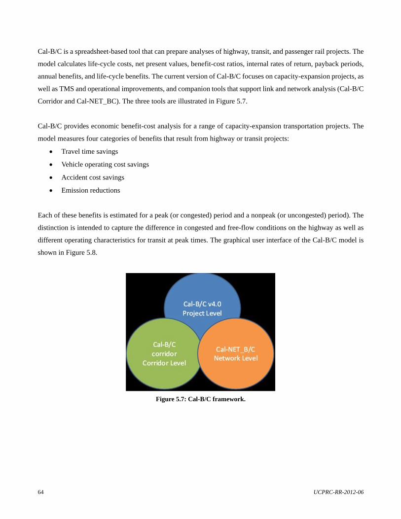
64 UCPRC-RR-2012-06
Cal-B/C is a spreadsheet-based tool that can prepare analyses of highway, transit, and passenger rail projects. The
model calculates life-cycle costs, net present values, benefit-cost ratios, internal rates of return, payback periods,
annual benefits, and life-cycle benefits. The current version of Cal-B/C focuses on capacity-expansion projects, as
well as TMS and operational improvements, and companion tools that support link and network analysis (Cal-B/C
Corridor and Cal-NET_BC). The three tools are illustrated in Figure 5.7.
Cal-B/C provides economic benefit-cost analysis for a range of capacity-expansion transportation projects. The
model measures four categories of benefits that result from highway or transit projects:
Travel time savings
Vehicle operating cost savings
Accident cost savings
Emission reductions
Each of these benefits is estimated for a peak (or congested) period and a nonpeak (or uncongested) period). The
distinction is intended to capture the difference in congested and free-flow conditions on the highway as well as
different operating characteristics for transit at peak times. The graphical user interface of the Cal-B/C model is
shown in Figure 5.8.
Figure 5.7: Cal-B/C framework.

UCPRC-RR-2012-06 65
Figure 5.8: Cal-B/C graphical user interface.
The output presents the final investment measures as well as annualized and life-cycle benefits and allows users to
include the effects of induced travel and vehicle emissions. Cal-B/C calculates induced travel benefits using
consumer surplus theory. Cal-B/C summarizes analysis results on a per-project basis using several measures:
Life-cycle costs
Life-cycle benefits
Net present value
Benefit/cost ratio
Rate of return on investment
Project payback period
Benefits are calculated for:
Travel time savings
Vehicle operating cost savings
Accident cost savings
Emission cost savings

66 UCPRC-RR-2012-06
Highway design and traffic data must be entered for highway projects. Statewide default values are provided for
some inputs. The following required inputs are deemed to be potentially affected by the work conducted in this
pilot study:
Roadway type—Indicate if the road is a freeway, expressway, or conventional highway in build and no
build cases.
Number of general traffic lanes—Indicate number of general-purpose lanes in both directions for build
and no build cases.
Number of HOV lanes—Indicate number of HOV lanes in both directions for the build and no build cases.
HOV restriction—If a highway facility has/will have HOV lanes, the HOV restriction needs to be
provided.
Highway free-flow speed—Indicate free-flow speed for build and no build cases.
Current average annual daily traffic (AADT)—Indicate current two-way AADT on facility.
Forecast AADT—Indicate projected AADT for 20 years after construction completion.
Hourly HOV/HOT volumes.
Percent trucks—Indicate estimated percentage of AADT made up of trucks.
Truck speed—Enter estimated speed for slow vehicles.
Pavement condition—Indicate base International Roughness Index (IRI).
5.3.6 Private Industry
Discussions were held with the California Trucking Association about potential interest and support from private
industry in the pilot study. Concerns were raised about the potential effects on the trucking industry, specifically
regarding potential increased fees and the long-term outcome of this pilot study. A standard boilerplate with
background to the pilot study and the objectives of the pilot study was shared with the focus on future
prioritization of maintenance work, potential economic impacts of rough roads on freight damage, and more
efficient utilization of existing maintenance funds.
The potential involvement of industry in Task 8 activities (measurement of truck and freight response on a range
of pavement types) was discussed. Potential involvement includes:
GPS tracking and acceleration measurements on selected trucks traveling on designated state highway
segments—need for trucks, trailers and freight
Truck trailer information as input into computer simulations of vehicles traveling over a range of
pavements

UCPRC-RR-2012-06 67
Decisions regarding privacy and confidentiality around collected data and operations were briefly discussed.
These issues may be dealt with through UC and other universities’ standard procedures. The proposed field work
procedure indicated in Section 6.3 was shared with the CTA to identify potential industry partners.
5.3.7 MIRIAM Project
The Models for rolling resistance In Road Infrastructure Asset Management systems (MIRIAM) project was
initiated by 12 partners from Europe and the United States with the objective of conducting research to provide
sustainable and environmentally friendly road infrastructure, mainly through reducing vehicle rolling resistance
and subsequently lowering CO2 emissions and increasing energy efficiency. In the first phase the focus is on
investigation of:
Pavement characteristics
Energy efficiency
Modeling
Raising awareness of the project to secure economic and political support for a second phase, during
which incorporation of CO2-controlling models into road infrastructure asset-management systems could
be developed and implemented
Potential links between the MIRIAM project and this pilot study mainly lie in the potential use of selected rolling
resistance models originating from MIRIAM in the evaluation of the effects of pavement roughness on vehicle
energy use, emissions, and rolling resistance.
The influencing parameters and potential energy losses that should be included in the concept of rolling resistance
form one of the important potential links between MIRIAM and this pilot study. Correlations are required between
rolling resistance coefficients or fuel consumption and road surface parameters to enable modeling of the concept
in PMS. Initial MIRIAM studies indicated that (29)
Rolling resistance is a property of tires and the pavement surface. In preliminary studies it was shown that
the rolling resistance coefficient for test tires increased by 21–55 percent due to changes in surface
roughness—corresponding to fuel consumption differences between 7 and 18 percent.
Macrotexture is a major factor influencing rolling resistance.
A substantial bias exists between various series of measurements made by presently available rolling
resistance trailers; temperature appears to be partly responsible for such differences.
It is proposed that a tentative source model for the pavement influence on rolling resistance contain mean
profile depth (MPD), pavement roughness (IRI), and pavement stiffness as significant pavement
parameters.
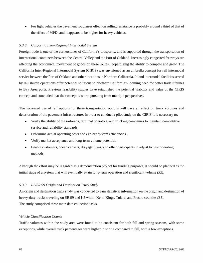
68 UCPRC-RR-2012-06
For light vehicles the pavement roughness effect on rolling resistance is probably around a third of that of
the effect of MPD, and it appears to be higher for heavy vehicles.
5.3.8 California Inter-Regional Intermodal System
Foreign trade is one of the cornerstones of California’s prosperity, and is supported through the transportation of
international containers between the Central Valley and the Port of Oakland. Increasingly congested freeways are
affecting the economical movement of goods on these routes, jeopardizing the ability to compete and grow. The
California Inter-Regional Intermodal System (CIRIS) was envisioned as an umbrella concept for rail intermodal
service between the Port of Oakland and other locations in Northern California. Inland intermodal facilities served
by rail shuttle operations offer potential solutions to Northern California’s looming need for better trade lifelines
to Bay Area ports. Previous feasibility studies have established the potential viability and value of the CIRIS
concept and concluded that the concept is worth pursuing from multiple perspectives.
The increased use of rail options for these transportation options will have an effect on truck volumes and
deterioration of the pavement infrastructure. In order to conduct a pilot study on the CIRIS it is necessary to:
Verify the ability of the railroads, terminal operators, and trucking companies to maintain competitive
service and reliability standards.
Determine actual operating costs and explore system efficiencies.
Verify market acceptance and long-term volume potential.
Enable customers, ocean carriers, drayage firms, and other participants to adjust to new operating
methods.
Although the effort may be regarded as a demonstration project for funding purposes, it should be planned as the
initial stage of a system that will eventually attain long-term operation and significant volume (32).
5.3.9 I-5/SR 99 Origin and Destination Truck Study
An origin and destination truck study was conducted to gain statistical information on the origin and destination of
heavy-duty trucks traveling on SR 99 and I-5 within Kern, Kings, Tulare, and Fresno counties (31).
The study comprised three main data collection tasks.
Vehicle Classification Counts
Traffic volumes within the study area were found to be consistent for both fall and spring seasons, with some
exceptions, while overall truck percentages were higher in spring compared to fall, with a few exceptions.

UCPRC-RR-2012-06 69
Truck Intercept Surveys
Little variance was observed in truck travel patterns between the fall and spring.
The majority of trucks (83.8 percent) were 5-axle double-unit type.
70 percent of the trucks were based within California. Of these, 47 percent were based in the San Joaquin
Valley region and 34 percent in the Southern California region.
The definitions of places where the trips originated from included:
o Shipper—Location where goods originate
o Consignee/receiver—Location where goods are delivered
o Yard—Place where trucks are stored and dispatched from
o Home—Residence of truck driver
o Port—Trips originating from and destined to ports of Los Angeles, Long Beach, and Hueneme
o Other
40.9 percent of the trips originated from a shipper and 36.9 percent from a yard. The percentage of other
locations dropped off significantly.
34.8 percent of the trips ended at a consignee/receiver, 27.4 percent at a yard, and 20 percent at a shipper.
The top five commodity types by percentage are:
o Food and similar products (21 percent)
o Empty trucks (18 percent)
o Farm products (14 percent)
o Miscellaneous freight (12 percent)
o Transportation equipment (4 percent)
Commercial Fleet Operator Survey
A commercial fleet operator survey of truck fleet operators provided information to obtain a better understanding
of commodities being transported in the corridors:
Truck operations are mostly local and regional, with trucks using SR 99 more often than I-5 due to origins
and destinations that cluster along SR 99.
Trucks tend to use I-5 to connect Kern County points with regions to the north and south (e.g., the Bay
Area or the Los Angeles Basin).
Regional trips place a burden on east-west connectors such as SR 166, SR 58, and SR 46.
Based on the origin-destination data, it is important to measure varying loads, as empty trucks respond differently
to pavement roughness than partially and fully loaded trucks, and thus incur a different level of wear and
maintenance.
70 UCPRC-RR-2012-06
5.3.10 State of Logistics South Africa
Selected extracts are provided (below) from the series of four South Africa State of Logistics articles that focused
on vehicle-pavement interaction issues. The original metric units are kept in this section, although imperial units
are provided where possible)
The Potential Cost of Bad Roads in South Africa (33)
The ride quality of a road has, for many years, been used as the primary indication of the quality of a road—mainly
due to findings that the most of the deterioration in the road structure ultimately translates into a decrease in the
riding quality of the road. Various studies about the effect of the ride quality of roads on the vibrations and
responses in vehicles have been conducted, with the main conclusions indicating that a decrease in the ride quality
of a road is a major cause of increased vibrations and subsequent structural damage to vehicles. These increased
vibrations and structural damage to vehicles can have many negative effects on the transportation cost of
companies and the broader economy of a country. The potential effects that worsening road conditions can have
on the broader economy are depicted in Figure 5.9.
Potential vehicle damage for vehicles traveling on uneven roads can only be addressed by mechanical engineers
through the improvement of the design of each vehicle traveling on the specific road. This immediately multiplies
the costs to a huge number of individual solutions. The poor quality of the road in this case, therefore, has an
increased cost effect on the vehicle and vehicle component design costs, manufacturing costs, and maintenance
costs. All these costs are typically incorporated into the cost that the vehicle owner charges to the customer for
transporting cargo, and therefore ride quality affects the logistical cost and ultimately the cost of goods to the
customer.
Figure 5.9: Potential effects of deteriorating road quality on the broader economy.
Increased vehicle damag
Increased fuel consumption
Increased logistics cost
Increased maintenance cost
Damage to transported cargo
Increasepackaging cost
Increased vehicle design and
manufacturing cost
Increased cost of transported cargo
Increased vehicle operating cost
Increased road loads
Increased road damages and
maintenance cost
Increased environmental
costs
Increased cost of
transported freight
Increased vehicle
operating cost
Increased environmental
cost

UCPRC-RR-2012-06 71
Driving on an uneven road surface affects the speeds at which the vehicle can travel safely, which immediately
affects the logistics of delivering goods at optimum times to a customer. A decrease in the ride quality of a road
causes a direct increase in the road maintenance cost. It also shortens the life of the road due to the increased
vibration of the vehicles, which in turn increases the dynamic component of the vehicle loads on the road. The
vibrations from the road are translated to the transported cargo, which results in damages to the cargo. Potential
solutions to this problem include improvements to the packaging of the cargo or improvements in the design of the
cargo itself. Decreases in ride quality also affect the environment and environmental costs through increased
vehicle operating costs and increased emissions due to slower speeds and longer durations of transport.
Congestion levels are very high in some areas, and the effect of this is that travel times, fuel consumption, and
emissions released into the environment increase.
A limited case study was conducted at a transportation company in South Africa to investigate the potential effect
of bad road surfaces on vehicle damages and costs. Anecdotal evidence was analyzed to obtain an indication of the
potential effect road condition could have on vehicle damage and costs. The analysis indicated that the trucks
traveling on the roads with worse ride conditions experience an increase in cost of between 685 percent and
1,560 percent, when moving from a road in good condition to an average- or poor-condition road (Table 5.7).
Table 5.7: Potential Increase in Vehicle Damage Cost under Deteriorating Road Conditions
Road Condition
Percent of Total Vehicle
Damages
Percent of Total Cost of Vehicle
Damages
Percent Increase in
Cost 2 (good) 5.2 3.9 3 (average) 17.4 30.8 684 4 (poor) 77.4 65.2 1,560
Cost of Bad Roads to the Economy (34)
Increased vehicle maintenance and repair cost leads to increased vehicle operating costs of transport operators. In
addition, worsening road conditions can result in increased vehicle vibrations, which may eventually translate into
increased damages to transported cargo. The transport operator may be held liable for any damages during the
transportation of goods. It therefore follows that on roads with deteriorating ride quality the transport operator
either has to take a loss or increase transport tariffs due to the higher operating costs. Consequently, the selling
price of products may increase, as the increased transportation cost must either be absorbed by the seller or
transferred to the consumer through increased prices.
To understand the potential effects of bad roads on the total logistics cost of companies, a case study was
conducted at two operating companies within a large logistics service provider in South Africa. The average repair
and maintenance cost of vehicles of the two companies traveling on specific routes, the associated IRI, and
condition rating of that route is shown in Table 5.8. Company A identified 10 trucks from its fleet traveling mostly
on the same route, and provided a database of actual maintenance and repair costs for the selected vehicles for

72 UCPRC-RR-2012-06
January–June 2008. Company B provided a database of its actual maintenance and repair costs for a fleet of
577 trucks operating on a range of roads in South Africa for January–September 2008,. For each company, similar
truck types were used to ensure that the route—and therefore the IRI—was the only factor of difference in the
analysis of the two companies. A graphical depiction of the potential increase in vehicle maintenance and repair
cost as a result of worsening road conditions is provided in Figure 5.10.
To investigate the impact that the increase in vehicle maintenance and repair cost may have on the total logistics
cost of a company, a further analysis is done in this section. A summary of the potential increase in vehicle
maintenance and repair cost when moving from a good road condition to a fair or to a bad road condition, as well
as the increase in the total logistics cost of a company as a result of worsening road conditions, can be seen in
Table 5.8.
Table 5.8: Summary of Vehicle Maintenance and Repair Cost for Routes with Different IRIs
Company Route Information Average IRI
(m/km)/[ft/mi]Road Condition
Rating
Average Maintenance and
Repair Cost (ZAR/km)
A Gauteng to Durban (N3)
2.7 [173] Good 1.01
Gauteng to Cape Town (N1) 3.6
[230] Fair 1.30
B
Gauteng to Durban (N3) 2.7
[173] Good 0.90
Gauteng to Nelspruit (N4) 2.9
[186] Fair 0.82
Gauteng to Witbank (N12) 3.4
[218] Fair 1.27
Gauteng to Rustenburg (N4) 3.3
[211] Fair 1.04Gauteng to Richardsbay (N17 and N2)
3.6 [230] Fair 1.31
Johannesburg to Vereeniging (R82)
3.6 [230] Fair 1.57
Gauteng to Cape Town (N12 and N1)
3.6 [230] Fair 1.29
Gauteng to Botswana (N4) 3.9
[250] Fair 1.35Newcastle to Gauteng (N11 and N17)
4.2 [269] Bad 2.09
Gauteng to construction sites 4.3
[275] Bad 2.13Note: ZAR = South African Rand

UCPRC-RR-2012-06 73
Figure 5.10: Potential increase in vehicle maintenance and repair cost due to bad roads.
Table 5.9: Summary of Potential Increases due to Worsening Road Conditions
Road Condition
Average Maintenance
and Repair Cost (ZAR/km)
Average Percentage Increase in Truck Maintenance and
Repair Cost
Average Percentage Increase
in Company Logistics Cost
Good 0.96 – – Fair 1.24 30.24 2.60 Bad 2.11 120.94 10.40
Note: ZAR = South African Rand
The increase in internal logistics costs due to inadequate road conditions is experienced by most, if not all,
transportation companies in a country. This figure eventually adds up to a massive increase in the logistics costs of
the country as a whole. As the logistics costs of a country increase, the cost of its products in the global
marketplace increases, which can have devastating effects on the global competitiveness of that country. It is
therefore of critical importance to manage logistics costs effectively and to minimize unnecessary costs that can
translate into higher product costs.
The Potential Effects of Deteriorating Road Quality and Maintenance in South Africa (35)
An evaluation of the potential negative effects of deteriorating road quality on transported cargo and the potential
effects of road maintenance on companies were conducted. Even though it may be argued that the potential
negative effects of bad roads warrant the proper maintenance and repair of the road network, it is important to
consider the potential effects and cost of maintaining the roads before deciding how to deal with any unwanted
effects.
0.00
0.05
0.10
0.15
0.20
0.25
0.30
0.35
0.40
0.45
0.50
0 100 200 300 400
Veh
icle
add
itio
nal r
epai
r an
d m
aint
enan
ce c
osts
[U
S$/m
ile]
Road roughness [inch/mile]

74 UCPRC-RR-2012-06
International studies indicate a link between the condition of a road and the vibrations experienced in a truck
traveling on that road. Different types of cargo (e.g., fresh produce and glass articles) are sensitive to different
vibration ranges and magnitudes. The vehicle type, properties, and operating speed also affect potential damage to
the cargo. Since excessive vibrations experienced by transported cargo can lead to cargo damage, it is important to
investigate the actual effects that increased vibrations—caused by bad roads—can have on transported cargo.
The vibrations experienced at specific positions in trucks traveling on the South African road network were
monitored to determine the relationship between damage to the transported cargo and road condition. The position
of cargo in the truck is important, as the dimensions of the truck will affect the level to which vibrations are
transposed to different areas in the truck. Current local and international investigations indicate that cargo situated
at the uppermost location at the back of the truck’s trailer experiences the highest levels of vibration and damage.
An example of the damage to fresh produce transported in the back of a trailer over roads with high roughness is
shown in Figure 5.11.
Figure 5.11: Typical damage to fresh produce cargo due to road roughness.
Analysis of satellite tracking data obtained from trucks operated on the route between Johannesburg and Port
Elizabeth—a distance of approximately 1,000 km (620 mi)—during 2010 indicated the following interesting
information. On a 50 km (31 mi) section of single-lane road where only one lane was available for traffic due to
road maintenance, the truck had to stop 18 times (for at least 10 minutes each time), and attained an average speed
of 20 km/h (12 mph). If the remainder of the road is assumed to be in a good condition and the truck can achieve
an average speed of 60 km/h (37 mph) for the good section of the route, the delay increases the travel time from
around 16.7 hours to 21.3 hours, a 27 percent increase in travel duration.
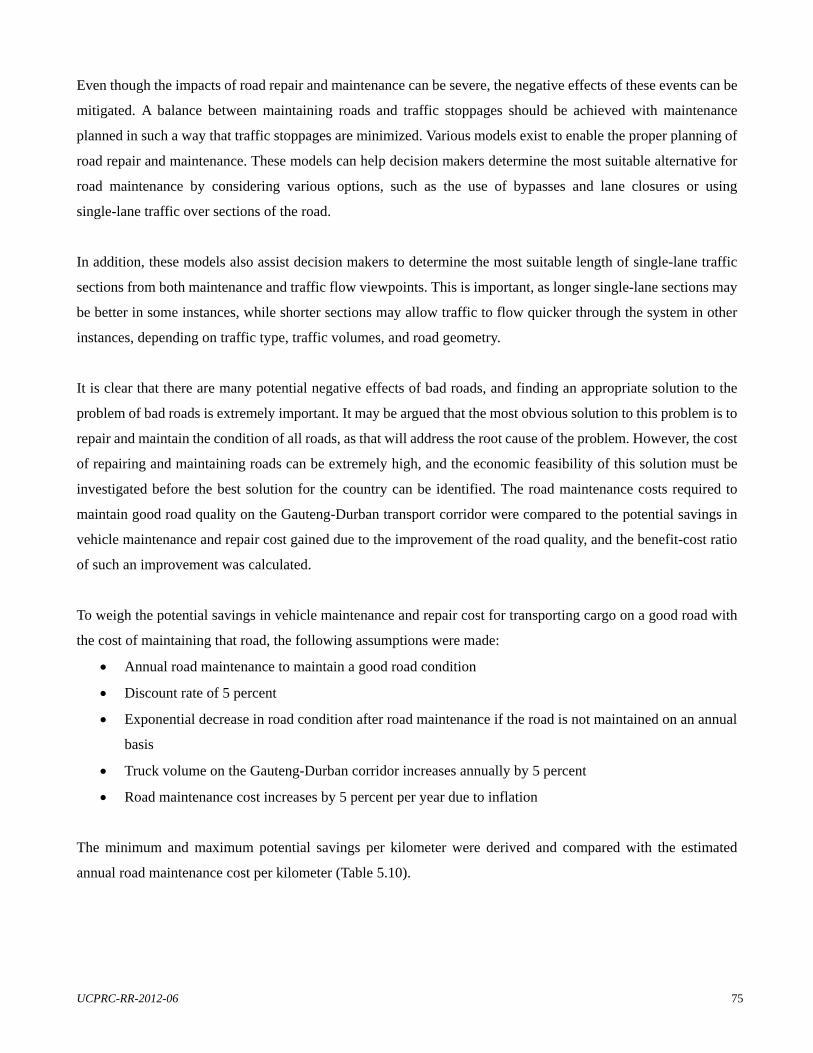
UCPRC-RR-2012-06 75
Even though the impacts of road repair and maintenance can be severe, the negative effects of these events can be
mitigated. A balance between maintaining roads and traffic stoppages should be achieved with maintenance
planned in such a way that traffic stoppages are minimized. Various models exist to enable the proper planning of
road repair and maintenance. These models can help decision makers determine the most suitable alternative for
road maintenance by considering various options, such as the use of bypasses and lane closures or using
single-lane traffic over sections of the road.
In addition, these models also assist decision makers to determine the most suitable length of single-lane traffic
sections from both maintenance and traffic flow viewpoints. This is important, as longer single-lane sections may
be better in some instances, while shorter sections may allow traffic to flow quicker through the system in other
instances, depending on traffic type, traffic volumes, and road geometry.
It is clear that there are many potential negative effects of bad roads, and finding an appropriate solution to the
problem of bad roads is extremely important. It may be argued that the most obvious solution to this problem is to
repair and maintain the condition of all roads, as that will address the root cause of the problem. However, the cost
of repairing and maintaining roads can be extremely high, and the economic feasibility of this solution must be
investigated before the best solution for the country can be identified. The road maintenance costs required to
maintain good road quality on the Gauteng-Durban transport corridor were compared to the potential savings in
vehicle maintenance and repair cost gained due to the improvement of the road quality, and the benefit-cost ratio
of such an improvement was calculated.
To weigh the potential savings in vehicle maintenance and repair cost for transporting cargo on a good road with
the cost of maintaining that road, the following assumptions were made:
Annual road maintenance to maintain a good road condition
Discount rate of 5 percent
Exponential decrease in road condition after road maintenance if the road is not maintained on an annual
basis
Truck volume on the Gauteng-Durban corridor increases annually by 5 percent
Road maintenance cost increases by 5 percent per year due to inflation
The minimum and maximum potential savings per kilometer were derived and compared with the estimated
annual road maintenance cost per kilometer (Table 5.10).

76 UCPRC-RR-2012-06
Comparing the estimated annual road maintenance costs per kilometer with the potential savings in vehicle
operating cost shows significant benefits that can be realized when keeping the road in a good condition. It is
important to note that only truck traffic volumes were used in this analysis; therefore the actual benefit-cost ratios
should be higher than the figures presented.
Table 5.10: Benefit-Cost Ratio of Keeping the Road in a Good Condition
Year Road Maintenance
Cost (ZAR/km)
Potential Savings (ZAR/km) Benefit-Cost Ratio
Minimum Maximum Minimum Maximum 1 600,000 (318,311) (79,163)
2 630,000 (156,763) 245,006
3 661,500 21,736 601,790
4 694,575 348,913 1,234,813
5 729,304 777,232 2,056,250
6 765,769 1,391,316 3,222,637
7 804,057 2,215,862 4,779,711
Total 4,279,985 12,061,043 1.88 3.47
Note: ZAR = South African Rand
The Potential Effects of Bad Roads on Transported Cargo(36)
This article presented two case studies that investigated the potential effects of deteriorating road quality on cargo
damages and losses. The distribution of fresh produce in the agriculture sector requires extensive handling and
transportation after harvesting—actions that can result in damage to and loss of products. This has significant
economic impact on the agriculture sector, as damaged produce have reduced economic value and losses decrease
revenue. The case studies investigated and quantified the additional damage to and loss of transported cargo
incurred when fresh produce is transported on bad (as opposed to good) roads.
In this sector, trucks travel on a variety of road types before reaching their destination. In most cases the first stage
of travel is on a gravel road from the farms where fresh produce is harvested. Gravel roads are generally in a worse
condition and are rougher than paved national and provincial roads. Therefore the majority of damage to fresh
produce and loss during transportation occurs while it is traveling on gravel roads.
The purpose of the fruit damage case study is to quantify the vibrations a truck and the fresh fruit it carries endure
due to different road conditions when traveling from growers in the Limpopo Province to market distributors in
Pretoria and Johannesburg. The vibrations generated during transport were then compared with vibration ranges
known to cause damage to transported produce. The case study considered six similar trucks and four types of fruit.
The trucks used in the case study traveled on national and provincial roads considered to be in good condition,
with IRI values of 0.8–2.5 m/km (51–160 ft/mi), and conversely on gravel roads that had not been regraveled in
the past eight years and had an IRI value of around 8 m/km (512 ft/mi).
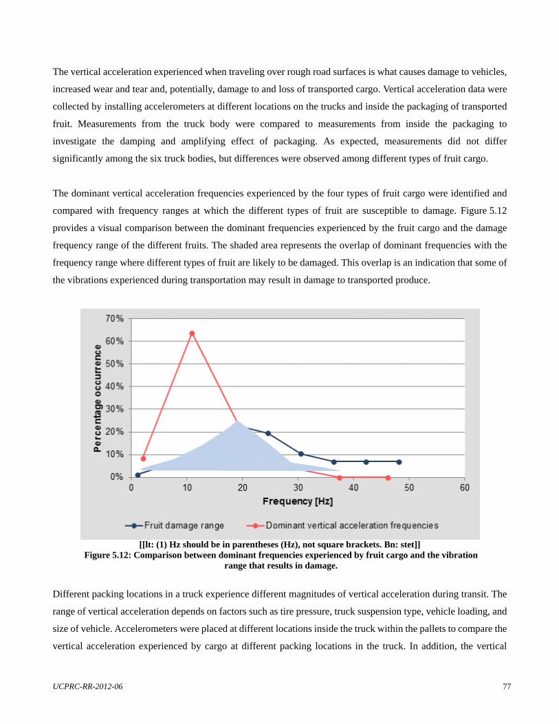
UCPRC-RR-2012-06 77
The vertical acceleration experienced when traveling over rough road surfaces is what causes damage to vehicles,
increased wear and tear and, potentially, damage to and loss of transported cargo. Vertical acceleration data were
collected by installing accelerometers at different locations on the trucks and inside the packaging of transported
fruit. Measurements from the truck body were compared to measurements from inside the packaging to
investigate the damping and amplifying effect of packaging. As expected, measurements did not differ
significantly among the six truck bodies, but differences were observed among different types of fruit cargo.
The dominant vertical acceleration frequencies experienced by the four types of fruit cargo were identified and
compared with frequency ranges at which the different types of fruit are susceptible to damage. Figure 5.12
provides a visual comparison between the dominant frequencies experienced by the fruit cargo and the damage
frequency range of the different fruits. The shaded area represents the overlap of dominant frequencies with the
frequency range where different types of fruit are likely to be damaged. This overlap is an indication that some of
the vibrations experienced during transportation may result in damage to transported produce.
[[lt: (1) Hz should be in parentheses (Hz), not square brackets. Bn: stet]]
Figure 5.12: Comparison between dominant frequencies experienced by fruit cargo and the vibration range that results in damage.
Different packing locations in a truck experience different magnitudes of vertical acceleration during transit. The
range of vertical acceleration depends on factors such as tire pressure, truck suspension type, vehicle loading, and
size of vehicle. Accelerometers were placed at different locations inside the truck within the pallets to compare the
vertical acceleration experienced by cargo at different packing locations in the truck. In addition, the vertical

78 UCPRC-RR-2012-06
acceleration experienced by the truck body was also measured. In general, pallets at the back of the truck and
pallets on top of the pallet stacks in the front and middle of the truck experienced higher acceleration.
Figure 5.13 displays the normalized distributions of the vertical accelerations experienced at various packing
levels in the front of the truck as well as on the truck body. The distributions for the accelerations experienced by
the bottom and middle levels are very similar to that of the truck body. It is evident from the slightly lower mean
value and variation of accelerations experienced in the bottom pallets compared to the truck body that the
packaging does dampen the vertical acceleration. Fruit packaged on fiberboard pallets on the bottom level in the
front of the truck were most protected against vibration damage incurred during transport.
Figure 5.13: Normalized distributions of the vertical accelerations experienced within pallets at various
packing levels at the front of the truck.
The economic impact of damaged agricultural cargo is absorbed differently by large- and small-scale farming
operations. Large operations either use in-house fleets or outsource to transportation companies. In the former
case, trucks can be customized for certain cargo or operational techniques can be enforced that mitigate damage
due to vibration. In the latter case, service-level agreements and insurance safeguard the farmers’ interests to a
great extent. Small-scale farmers are typically more vulnerable, as they generally provide their own transport and
thus are not safeguarded by service-level agreements or insurance and, unlike with large fleets, their vehicles,
packaging, and operational procedures are not customized to moderate cargo damage.
Normalized (g)
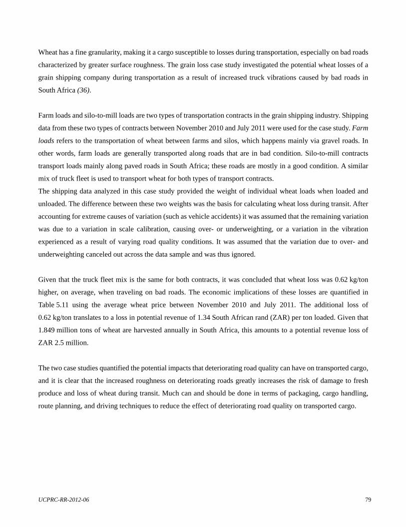
UCPRC-RR-2012-06 79
Wheat has a fine granularity, making it a cargo susceptible to losses during transportation, especially on bad roads
characterized by greater surface roughness. The grain loss case study investigated the potential wheat losses of a
grain shipping company during transportation as a result of increased truck vibrations caused by bad roads in
South Africa (36).
Farm loads and silo-to-mill loads are two types of transportation contracts in the grain shipping industry. Shipping
data from these two types of contracts between November 2010 and July 2011 were used for the case study. Farm
loads refers to the transportation of wheat between farms and silos, which happens mainly via gravel roads. In
other words, farm loads are generally transported along roads that are in bad condition. Silo-to-mill contracts
transport loads mainly along paved roads in South Africa; these roads are mostly in a good condition. A similar
mix of truck fleet is used to transport wheat for both types of transport contracts.
The shipping data analyzed in this case study provided the weight of individual wheat loads when loaded and
unloaded. The difference between these two weights was the basis for calculating wheat loss during transit. After
accounting for extreme causes of variation (such as vehicle accidents) it was assumed that the remaining variation
was due to a variation in scale calibration, causing over- or underweighting, or a variation in the vibration
experienced as a result of varying road quality conditions. It was assumed that the variation due to over- and
underweighting canceled out across the data sample and was thus ignored.
Given that the truck fleet mix is the same for both contracts, it was concluded that wheat loss was 0.62 kg/ton
higher, on average, when traveling on bad roads. The economic implications of these losses are quantified in
Table 5.11 using the average wheat price between November 2010 and July 2011. The additional loss of
0.62 kg/ton translates to a loss in potential revenue of 1.34 South African rand (ZAR) per ton loaded. Given that
1.849 million tons of wheat are harvested annually in South Africa, this amounts to a potential revenue loss of
ZAR 2.5 million.
The two case studies quantified the potential impacts that deteriorating road quality can have on transported cargo,
and it is clear that the increased roughness on deteriorating roads greatly increases the risk of damage to fresh
produce and loss of wheat during transit. Much can and should be done in terms of packaging, cargo handling,
route planning, and driving techniques to reduce the effect of deteriorating road quality on transported cargo.
80 UCPRC-RR-2012-06
Table 5.11: Comparison of Average Wheat Loss on Good and Bad Roads Wheat Loss by Weight
Road Condition Rating
Load Weight (ton)
Loss per Load
(kg)/[lb]
Loss per Ton Loaded (kg/ton)
Difference (kg/ton)
Road Condition
Rating Load Weight
(ton)
Loss per Load
(kg)/[lb] Good 34.71 36.09
[79] 1.04 – Good
34.7136.09
[79]Bad 22.86 37.85
[84] 1.66 0.62 Bad
22.8637.85
[84]Wheat Loss in Rand (average values)
Road Condition Rating
Wheat Price (ZAR/ton)
Loss per Ton Loaded
(kg)
Value Lost per Ton Loaded
(ZAR) Difference
(ZAR)
Road Condition Rating
Wheat Price (ZAR/ton)
Loss per Ton Loaded
(kg) Good 2,167.82 1.04 2.25 – Good 2,167.82 1.04Bad 2,167.82 1.66 3.59 1.34 Bad 2,167.82 1.66Notes: ton = metric ton (1,000 kg); ZAR = South African Rand
5.3.11 Other Regions and Corridors
Apart from the information presented in this section there was no substantial and detailed information found on
regions or corridors apart from the San Joaquin Valley that could add to the discussions in this report.
5.4 Freight Logistics Analysis
5.4.1 Introduction to Freight Logistics and the Broader Supply Chain
A supply chain is more than just the operations required to move goods from one company to the next. More
accurately, supply chain comprehensively describes the movement of materials from the source (raw materials) to
the consumer/end customer (final products/services). Typically, a number of companies are involved in a supply
chain, each fulfilling different operations or providing planning and management services to the supply chain. A
supply chain encompasses purchasing, manufacturing, warehousing, transportation, customer service, demand
planning, supply planning, information exchange, and management services. Considered in its entirety, a supply
chain constitutes people, processes, materials, equipment, and information. Freight logistics is typically focused
on the processes and elements in the supply chain that move materials from one geographic location in the supply
chain to another. Although physical transportation is the greatest component of freight logistics, fleet management,
transport planning, distribution strategies, transport packaging, route planning, freight inspection, and so forth are
also constituents of the broader freight logistics function.
The Supply Chain Operations (SCOR®) Framework is a standard model used to map and describe supply chains.
The SCOR Framework is a product of the Supply Chain Council (www.supply-chain.org) and is a recognized
industry standard. Figure 5.14 is based on the SCOR model and shows a simplified schematic of a supply chain
and its freight logistics interfaces. Consider, for example, the following simplified explanation of a tomato
processing supply chain where the raw materials (fresh tomatoes) are grown in California and processed locally
and then the final product (processed tomatoes) is sold in California or neighboring states.
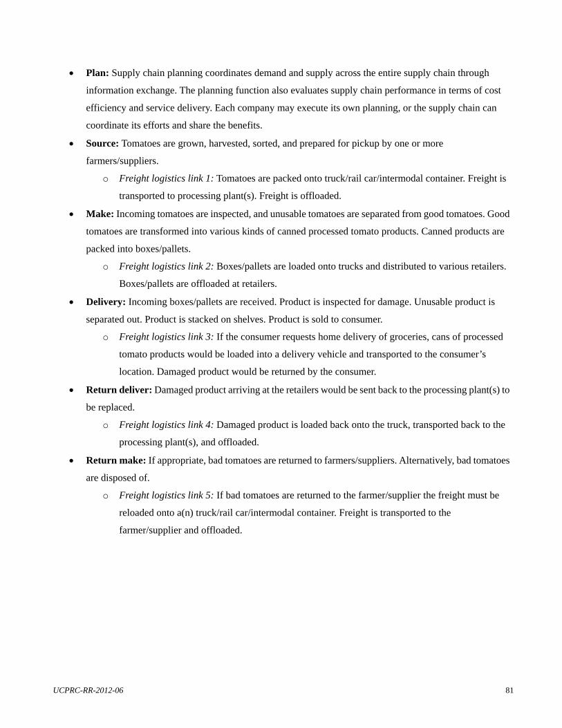
UCPRC-RR-2012-06 81
Plan: Supply chain planning coordinates demand and supply across the entire supply chain through
information exchange. The planning function also evaluates supply chain performance in terms of cost
efficiency and service delivery. Each company may execute its own planning, or the supply chain can
coordinate its efforts and share the benefits.
Source: Tomatoes are grown, harvested, sorted, and prepared for pickup by one or more
farmers/suppliers.
o Freight logistics link 1: Tomatoes are packed onto truck/rail car/intermodal container. Freight is
transported to processing plant(s). Freight is offloaded.
Make: Incoming tomatoes are inspected, and unusable tomatoes are separated from good tomatoes. Good
tomatoes are transformed into various kinds of canned processed tomato products. Canned products are
packed into boxes/pallets.
o Freight logistics link 2: Boxes/pallets are loaded onto trucks and distributed to various retailers.
Boxes/pallets are offloaded at retailers.
Delivery: Incoming boxes/pallets are received. Product is inspected for damage. Unusable product is
separated out. Product is stacked on shelves. Product is sold to consumer.
o Freight logistics link 3: If the consumer requests home delivery of groceries, cans of processed
tomato products would be loaded into a delivery vehicle and transported to the consumer’s
location. Damaged product would be returned by the consumer.
Return deliver: Damaged product arriving at the retailers would be sent back to the processing plant(s) to
be replaced.
o Freight logistics link 4: Damaged product is loaded back onto the truck, transported back to the
processing plant(s), and offloaded.
Return make: If appropriate, bad tomatoes are returned to farmers/suppliers. Alternatively, bad tomatoes
are disposed of.
o Freight logistics link 5: If bad tomatoes are returned to the farmer/supplier the freight must be
reloaded onto a(n) truck/rail car/intermodal container. Freight is transported to the
farmer/supplier and offloaded.

82 UCPRC-RR-2012-06
Figure 5.14: Simplified schematic of a supply chain.
5.4.2 Freight Damage as a Result of V-PI
Each of the freight logistics links indicates a position in the supply chain where V-PI could potentially damage
freight. Two primary types of freight damage are:
Freight damage due to vibration motion or sudden jolts. This includes “mechanical failure, fatigue
failure, cosmetic damage, undesirable settling of contents, breaking up between solid/liquid suspensions,
static charge buildup, bottle-closure cap back-off and leaking fluids and powdered products” (37).
Freight loss due to vibration. This is relevant to grain, natural sands, and other mining related freight
that can fall through cracks in the truck body, particularly when aggravated by abnormal vibration.
Steyn et al. (36) investigated both of these types of freight damage in the South African context through case
studies published in the Eighth State of LogisticsTM Survey for South Africa 2011 (see Section 5.3.10 for
description and references).
A third potential impact could be that, under severe conditions, the equipment on the truck body intended to
maintain freight integrity is damaged; for example, the cooling unit on a truck might be damaged by vibrations and
jolts, affecting the integrity of the entire shipment. However, this is considered a high-impact, low-probability
event.
The further along the supply chain, the more costly it is to write off freight. A pound of fresh tomatoes costs less to
write off than a pound of processed product. Three typical supply chain responses to freight damage are:
Product is sent back to the shipper for replacement, repair, or repackaging—placing a burden on the
reverse supply chain (e.g., manufactured or electronic products);.Product is written off and must be
disposed of by the receiver (e.g., damaged agricultural products).
Product must be reclassified before selling (e.g., downgrading fruit).
UCPRC-RR-2012-06 83
All three of these freight damage responses require additional accounting and information exchange procedures,
creating an additional administrative burden. The true cost of freight damage is thus the sum of the lost revenue
and the cost of the operational repercussions caused.
There are many ways to prevent freight damage or mitigate the effects thereof. Protective packaging, freight
insurance, customized trucks, and route avoidance (deliberately choosing alternative routes to avoid a particular
stretch of road) are typical mechanisms employed.
Packaging engineering is an established discipline in which much attention is given to designing and testing
packaging that protects products during transport and material handling. In the past few decades countless studies
have been conducted to quantify the effect of transport vibrations on agricultural freight and compare the
protection offered by various types of packaging. However, literature pertaining to the freight damage incurred by
manufactured/processed goods and other nonagricultural commodities is scant. Agricultural freight is fragile and
thus deserving of protective packaging, but it is a low-value, low-margin product that does not justify excessive
spending on transport packaging. Therefore freight damage due to transport vibrations is a common occurrence in
the agricultural industry. In fact, it is estimated that 30 to 40 percent of produce is discarded between the grower
and consumer due to damage (38). Manufacturers, on the other hand, go to great lengths to protect their final
products through packaging—especially for high-value goods. The lack of freight damage literature related to
manufactured goods could thus be because of the relatively low occurrence of freight damage during transport or
because manufacturers do not want to publish research that could undermine their competitive advantage.
Studying the effects of V-PI on the freight logistics industry in California by quantifying the increase in vehicle
operating costs and freight damage costs (both direct and indirect) holds significant value for industry players.
Understanding these effects and having substantive proof of the relationship between pavement quality and supply
chain costs could afford industry players the following benefits:
Better-informed negotiations regarding freight insurance
Better-informed supplier selection and contracting decisions
Information for benefit-cost analyses related to transport packaging and customized vehicles
Information for benefit-cost analyses related to route avoidance strategies (e.g., Is the cost of taking a
longer route to avoid a bad stretch of road justified by the expected prevention of freight damage?)
Better-informed fleet management strategies—incorporating VPI effects into decisions about suspension
type and axles
Guidelines on how to best load truck bodies or intermodal containers to prevent freight damage

84 UCPRC-RR-2012-06
5.4.3 Pilot Study Objectives
The purpose of this pilot study is to investigate and quantify vehicle operating and freight damage costs due to the
VPI experienced on road surfaces of varying ride quality along freight routes within a specific area of California.
In particular, the results of this pilot study should illustrate the value of conducting a similar statewide study that
could inform road maintenance and repair planning. From a freight logistics point of view, it is implied that the
pilot study should show how freight damage costs can be investigated and quantified for specific commodity
flows within a study area.
It is important that the outcomes of this pilot study link with various ongoing studies and economic models as
detailed in Sections 1 and 5.5.
The most prominent implication for the freight logistics aspect is the link to the Cal-B/C model described in
Section 5.3.5. To perform a benefit-cost analysis of upgrading/repairing a certain stretch of road, potential freight
damage savings accrued by the upgrade must be given as input into the Cal-B/C model. Therefore, the pilot study
should develop a methodology whereby field measurements, stakeholder engagements, and existing data sources
can be used to estimate freight damage savings along a certain stretch of road.
5.4.4 Information Requirements to Calculate Freight Damage Costs
To achieve the objectives discussed above requires cost calculations at a disaggregate level. Firstly, the expected
freight damage cost incurred by a particular type of shipment must be quantified. Secondly the individual
shipment costs must be aggregated to provide higher-level cost estimates. Performing the cost calculation at the
disaggregate level requires the following steps:
Quantifying the probability and extent of freight damage incurred by a shipment traveling on a road
surface of a specific ride quality. This damage will depend on the vibration as influenced by road
roughness, distance, traveling speed, load, suspension type and number of axles, as well as specific
properties of the freight and its packaging (39).
Defining the indirect operational costs incurred due to freight damage. This will depend on the specific
supply chain in question.
Combining items 1 and 2 to obtain a total cost.
There is a significant body of knowledge relating to the freight damage caused by transport vibrations to specific
agricultural products including the following products:
Peaches
Apples

UCPRC-RR-2012-06 85
Pears
Apricots
Grapes
Loquats
Strawberries
Tomatoes
Potatoes
Oranges
Eggs
Unfortunately, the same cannot be said for manufactured and other nonagricultural goods. This means that in the
case of agricultural commodities, results and findings from previous studies could be used to fill knowledge gaps
in the data resulting from field measurements and industry interaction. In the case of nonagricultural or
manufactured goods the project team would rely heavily on data collected through field measurement. During the
field measurements, freight inspections at origin and destination would be required, in addition to the output from
the accelerometers, GPS, and other onboard equipment.
The literature studied shows that the practice of using freight damage results generated from vibration table
experiments instead of actual on-truck measurements is an acceptable methodology. The methodology is as
follows:
1. Collect statistically significant data about the vibrations experienced by loaded truck bodies while
traveling over varying pavement conditions through field measurements.
2. Create vibration profiles from these field measurements as input to the vibration table, which will emulate
the vibration experienced on the floor of the truck body.
3. Stack freight onto the vibration table as it would be done in the truck (i.e., use the same packaging, stack
height, etc.).
4. Vibrate the freight according to the vibration profiles.
5. Inspect freight and record freight damage.
This methodology can be repeated for many different kinds of freight, packaging methods, and stacking profiles,
thus greatly reducing the number and variety of field measurements required. The University of Pretoria has
vibration table equipment both in the civil and mechanical engineering faculties.

86 UCPRC-RR-2012-06
Addressing item 2 (above) will require extensive stakeholder interaction to understand the state of practice for
various commodities in California and its neighboring states. This interaction could be achieved through
interviews with logistics managers and/or observing logistics operations at shipping and receiving facilities.
Aggregating freight damage costs within a study area for a certain time period would require knowing the volumes
of various types of freight transported over particular routes in a certain time period. Knowing the typical
shipment characteristics along a particular route —such as packaging and loading variation—would also refine
the damage and cost estimations, as these have a significant impact on the probability and degree of freight
damage.
5.4.5 Selecting a Preferable Study Area and Freight Types for the Pilot Study
This section identifies a preferable study area and freight types from a freight logistics point of view based on
information sources available to this pilot study (Section 5.3, Table 5.1 and Table 5.2).
Figure 5.15 is based on Table 5.1 (Summarized shipment characteristics by mode of transportation for state of
origin—) and shows the percentage of the total ton-miles, tons, and monetary value attributed to each commodity.
The commodities are sorted according to their ton-mile percentages. Table 5.12 lists the commodity descriptions
associated with the index numbers on the x-axis. Those commodities that are known to be susceptible to damage
due to bad road quality are italicized in the table. Mixed freight and miscellaneous manufactured products cover a
broad range of items that may or may not be susceptible; therefore they are also highlighted (italicized).
From Figure 5.15 the following commodities (susceptible to damage) stand out:
Other prepared foodstuffs and fats and oils—many tons and ton-miles shipped.
Other agricultural products—many ton-miles shipped.
Nonmetallic mineral products, gravel and crushed stone, coal and petroleum products—many tons
shipped.
Electronic and other electrical equipment and components and office equipment—high-value items.
Damage to a small proportion of freight could have great monetary implications.
UCPRC-RR-2012-06 87
Figure 5.15: Comparison of different commodity shipments originating from California. (See Table 5.12 for description of index designations in this figure.)
Table 5.12: Commodity Classes Associated with Figure 5.15Index Description Index Description 1 Other prepared foodstuffs and fats and oils 14 Chemical products and preparations 2 Nonmetallic mineral products 15 Gravel and crushed stone 3 Other agricultural products 16 Base metal in primary or semifinished forms
and in finished basic shapes 4 Motorized and other vehicles (including
parts) 17 Articles of base metal
5 Alcoholic beverages 18 Grains, alcohol, and tobacco products 6 Electronic and other electrical equipment
and components and office equipment 19 Animal feed and products of animal origin
7 Plastics and rubber 20 Meat, fish, seafood, and their preparations 8 Mixed freight 21 Basic chemicals 9 Textiles, leather, and articles of textile or
leather 22 Paper or paperboard articles
10 Miscellaneous manufactured products 23 Nonmetallic minerals 11 Coal and petroleum products 24 Fuel oils 12 Wood products 25 Pulp, newsprint, paper, and paperboard 13 Gasoline and aviation turbine fuel 26 Fertilizers
A similar analysis was done using the categories listed in Table 5.2 which compares commodities shipped on truck
for specified NCAIS-designated industries. The top 29 commodities (based on ton-miles) are shown in
Figure 5.16 and Table 5.13. From Figure 5.16 the following commodities (susceptible to damage) stand out:
0
2
4
6
8
10
12
14
16
18
20
0 1 2 3 4 5 6 7 8 9 10 11 12 13 14 15 16 17 18 19 20 21 22 23 24 25 26
Index for two-digit commodity types
2007 Value [%] 2007 Tons [%] 2007 Ton-miles [%]
Per
cen
tage
of
tota
l com
mod
itie
s or
igin
atin
g in
Cal
ifor
nia

88 UCPRC-RR-2012-06
Manufacturing, wholesale trade, merchant wholesalers, nondurable goods, food
manufacturing—relatively high tons and ton-miles
Nonmetallic mineral product manufacturing, mining (except oil and gas)—relatively many tons
Commodities that are known to be susceptible to damage due to bad road quality are highlighted (italicized) in
Table 5.13.
Therefore, when studying the effect of freight damage on road in California, the following commodities are most
relevant:
Various kinds of manufactured goods—particularly nondurable or electronic goods
Agricultural and various other food products
Mining products—coal, minerals, gravel
Figure 5.16: Comparison of different commodity shipments on truck in California.
0%
5%
10%
15%
20%
25%
30%
0 1 2 3 4 5 6 7 8 9 10 11 12 13 14 15 16 17 18 19 20 21 22 23 24 25 26 27 28 29
Per
cen
tage
of
tota
l com
mod
itie
s sh
ipp
ed o
n t
ruck
in
Cal
ifor
nia
Index for NAICS commodity types
2007 Value [%] 2007 Tons [%] 2007 Ton-miles [%]
UCPRC-RR-2012-06 89
Table 5.13: Commodity Types Associated with Figure 5.16
Index Industry Index Industry1 Manufacturing 16 Primary metal manufacturing 2 Wholesale trade 17 Petroleum and petroleum products merchant
wholesalers 3 Merchant wholesalers, nondurable
goods 18 Miscellaneous nondurable goods merchant
wholesalers 4 Food manufacturing 19 Transportation equipment manufacturing 5 Merchant wholesalers, durable goods 20 Beverage and tobacco product manufacturing 6 Chemical manufacturing 21 Petroleum and coal products manufacturing 7 Miscellaneous durable goods merchant
wholesalers 22 Chemical and allied products merchant
wholesalers 8 Grocery and related product merchant
wholesalers 23 Fabricated metal product manufacturing
9 Paper manufacturing 24 Lumber and other construction materials merchant wholesalers
10 Nonmetallic mineral product manufacturing
25 Machinery manufacturing
11 Corporate, subsidiary, and regional managing offices
26 Electrical equipment, appliance, and component manufacturing
12 Mining (except oil and gas) 27 Machinery, equipment, and supplies merchant wholesalers
13 Warehousing and storage 28 Farm product raw material merchant wholesalers
14 Wood product manufacturing 29 Other industries 15 Plastics and rubber products
manufacturing
From Table 5.1 it is also clear that for-hire trucks are responsible for a much greater proportion of ton-miles
traveled than in-house fleets. It is thus recommended that targeting transport providers or third-party logistics
providers (3PLs) (companies to which logistics processes are outsourced) for pilot study participation may be
more fruitful than only targeting in-house fleets.
Detailed studies on the San Joaquin Valley (Section 5.3.3) show that this valley has large agricultural, mining, and
manufacturing industries. In addition, almost half of the freight shipped in the valley has origin-destination pairs
within the valley (i.e., internal shipments) which would make shipment inspections easier. The tomato-growing
sector may be one sector to target, as tomatoes are fragile (soft) products. The dairy sector is not such an attractive
research focus from a freight damage point of view, as highly regulated, customized trucks, and durable packaging
make it unlikely that freight damage is incurred. However, from a VOC point of view it makes sense to investigate
the dairy sector.
Some logistics-related issues that need to be dealt with during the planning of the remainder of the tasks in this
pilot study include:
90 UCPRC-RR-2012-06
The impact of the vertical vibrations on the truck body are very different when the truck is fully loaded as
opposed to when the truck is empty or partially loaded (40). Load consolidation, truckload (TL) vs.
less-than-truckload (LTL), and empty backhauls are very important logistics issues that enjoy a lot of
attention. Shippers may be interested to know just how much of a difference the loading of their trucks
makes to the risk of cargo damage, fuel consumption, and maintenance costs.
Reducing fuel consumption is a major focus area in the “greening” of logistics, and the quantification of
differences in fuel consumption when traveling on roads with different roughness can add an extra data
element to the modeling of the problem.
From a business relationship point of view, it may be useful to understand “who pays” for the additional
maintenance and freight damage in a certain industry. If transport is mostly outsourced it would be the
trucking companies that incur the maintenance cost and then pass it on to their clients. If consignees take
ownership of the cargo when it leaves the consignor’s warehouse docks, the freight damage is incurred by
the consignee and never by the consignor. These kinds of insights would be useful to a supply chain
manager when planning upstream and downstream relationships.
It may be useful to compare freight damage in truck bodies (semitrailers) to that of freight packed in
intermodal containers that are then loaded onto truck trailers. Such insights and information could be very
useful when assessing intermodal freight logistics (i.e., combinations of rail and road transport).
5.5 Links, Inputs, and Outputs
Many potential sources of information have been presented in Sections 3, 4, and 5 of this report. It is important to
evaluate whether these sources link to each other and potentially support a uniform view of the issues around V-PI
effects on the broader economy of California. In Section 6.2 this data consolidation view is provided by means of
extracting major issues obtained from each of the sources and demonstrating how they link with each other and
support the objectives of the pilot study.
In discussions with potential organizations and parties that may assist in providing information for the pilot study,
a standard boilerplate was used as background to the study. This was mainly done to ensure that all parties outside
of the pilot study team could get a detailed and complete picture of the objectives and focus of the pilot study.
UCPRC-RR-2012-06 91
6 DISCUSSION 6.1 Introduction
This section focuses on the consolidation of the data in the previous chapters, as well as the development of
recommendations for further work in the project. Further, it allows for comments from the Caltrans project team
regarding the recommendations and for documenting the final decision on the corridor/route on which the pilot
study will be conducted.
6.2 Data Consolidation
6.2.1 Introduction
The data that were presented in discussed in Sections 3 to 5 of this document represent information sourced from
a range of independent sources. Each of the sets of information has been discussed in detail individually. In this
section a motivation is developed for the proposed Caltrans decision in Section 6.3 for a corridor/route to focus on
during the next phase of this pilot project. Therefore, relevant bits of information from Sections 3 to 5 are
combined to present a case. All the details from the specific data sets are not repeated, but reference is made to the
relevant sources and locations in the report.
6.2.2 Report Issues
The purpose of this pilot study is to provide data and information that will provide input that supports Caltrans’
freight program plans and related legislation with findings potentially contributing to economic evaluations;
identification of challenges to stakeholders; and identification of problems, operational concerns, and strategies
that “go beyond the pavement,” including costs to the economy and the transportation network (delay, packaging,
environment, etc.). Findings could lead to improved pavement policies and practices such as strategic
recommendations that link pavement surface profile, design, construction, and preservation with V-PI. These
findings also should provide information for evaluating the relationship between pavement ride quality (stemming
from the pavement’s condition), vehicle operating costs, freight damage, and logistics.
The overall objectives of this project are to enable Caltrans to better manage the risks of decisions regarding
freight and the management and preservation of the pavement network, as the potential effects of such decisions
(i.e., to resurface and improve ride quality earlier or delay such a decision for a specific pavement) will be
quantifiable in economic terms. This objective will be reached through applying the principles of
vehicle-pavement interaction (V-PI) and state-of-the-practice tools to simulate and measure peak loads and
vertical acceleration of trucks and their freight on a selected range of typical pavement surface profiles on the State
Highway System (SHS) for a specific region or Caltrans district.

92 UCPRC-RR-2012-06
The objectives of this report are to provide information on Tasks 1–6, and to provide guidance about the specific
corridor or district on which the pilot study (Tasks 7–12) should be focused.
Road Inventory
The main outcome of Task 3 is to identify routes in each district and county for which ride quality data exists, as
well as the actual ride quality for these routes (due to the volume of data, the actual data are kept only in electronic
form). Routes in California have been identified, and a database containing actual road profiles and ride quality
data is available for use in the remainder of the pilot project.
Vehicle Inventory
The deliverable for Task 4 is a table of current vehicle population per standard FHWA vehicle classifications for
Caltrans. Based on the various sources used in this task (FWHA truck classifications, commodity flow analysis,
and WIM data), the following was identified:
The most common truck types are FHWA Class 9 and 12 (up to 48 percent of the trucks on selected
routes), followed by Class 5.
High truck flows are experienced in District 6 – part of the San Joaquin Valley.
Axle load spectra are heavier at night than in the daytime.
Axle load spectra and truck type distribution show very little seasonal variation.
Axle load spectra are much higher in the Central Valley than in the Bay Area and Southern California,
particularly for tandem axles.
More than 90 percent of the truck traffic traveled in the outside or two outside lanes, on two- and
three-lane highways, respectively.
Truck speeds typically fall within the range of 50–75 mph (80–120 km/h).
Leaf springs are predominantly used in steering axles, with drive axles using air suspension and trail axles
using leaf suspension.
Information Review
Task 5 focuses on evaluating the data obtained from the various resources for Tasks 3–4, as well as additional
relevant information that may add to the project. The deliverable for Task 5 is a detailed understanding and input
to the progress report on the available data sources and required analyses for the project, inclusive of indications of
the potential links between the outputs from this project and the inputs for the various economic and planning
models.

UCPRC-RR-2012-06 93
California Statewide Freight Planning
The purpose of the California Statewide Freight Planning (CSFF) model is to provide a policy-sensitive model to
forecast commodity flows and commercial vehicle flows within California, addressing socioeconomic conditions,
land-use policies related to freight, environmental policies, and multimodal infrastructure investments. It requires
appropriate information and data about freight movements and costs to enable accurate modeling.
Commodity Flow Survey
It is evident that truck-based transportation dominates the freight transportation scene in California. Eighty-two
percent of the freight tons shipped from California utilizes only trucks. The data indicate that the highest
percentage of commodities and industries (in terms of value, tons, and ton-miles) transported by truck are
manufacturing goods, wholesale trade, and nondurable goods for the whole of California. No specific information
for commodity flows into California (destination California) could be identified in this pilot study.
San Joaquin Information
The San Joaquin Valley is composed of eight counties and 62 cities. It has a diverse internal economy and also
plays a major role in the distribution of agricultural materials throughout California, the United States, and the
world. Trucks are the dominant mode choice, with more than 450 million tons of goods moved by truck into, out
of, or within the San Joaquin Valley in 2007—more than 85 percent of all tonnage associated with these types of
moves in the San Joaquin Valley. Truck movement in the San Joaquin Valley relies on a combination of all levels
of highways and roads in the area. Key regional highways include the primary north-south corridors (I-5 and
SR 99) and east-west corridors (I-580, SR 152, SR 41, SR 46, and SR 58) and in total constitute more than
31,000 lane-miles. There are more than 2,700 lane-miles of truck routes in the San Joaquin Valley region, with in
excess of 80 percent designated STAA National Truck Routes.
Farm products are the dominant commodity carried outbound from the San Joaquin Valley, comprising 33 percent
of the total outbound movements. This consists of fresh field crops (vegetables, fruit and nuts, cereal grains, and
animal feed). Stone and aggregates account for 18 percent of the total, food and tobacco products around
10 percent, and waste and mixed freight 6 percent and 4 percent of the total tonnage, respectively.
The region accounts for over 8 percent of the total GDP for the state of California. However, the region accounts
for a much higher proportion of output within sectors such as agriculture (nearly 50 percent) and mining and
mineral extraction (25 percent). The San Joaquin Valley includes 6 of the top 10 counties in California for total
value of agricultural production.

94 UCPRC-RR-2012-06
Goods Movement Action Plan
The California Goods Movement Action Plan (GMAP) includes a compiled inventory of existing and proposed
goods movement infrastructure projects, including previously identified projects in various regional
transportation plans and regional transportation improvement programs prepared by metropolitan planning
organizations, regional transportation planning agencies, and county transportation commissions. One of the four
priority regions and corridors identified in the GMAP is the Central Valley region that includes the San Joaquin
Valley.
California Life-Cycle Benefit/Cost Analysis Model
Caltrans uses the California Life-Cycle Benefit/Cost Analysis Model (Cal-B/C) to conduct investment analyses of
projects proposed for the interregional portion of the State Transportation Improvement Program (STIP), the State
Highway Operations and Protection Program (SHOPP), and other ad hoc analyses requiring benefit-cost analysis.
The following required inputs are deemed to be potentially affected by the work conducted in this pilot study:
roadway type, number of general traffic lanes, number of HOV lanes, HOV restriction, highway free-flow speed,
current and forecast average annual daily traffic (AADT), hourly HOV/HOT volumes, percent trucks, truck speed,
and pavement condition.
Industry
Potential involvement of industry in Task 8 activities includes:
GPS tracking and acceleration measurements on selected trucks traveling on designated State Highway
segments—need for trucks, trailers and freight
Truck trailer information as input into computer simulations of vehicles traveling over a range of
pavements
Models for Rolling Resistance In Road Infrastructure Asset Management Systems Project
The objective of the Models for rolling resistance In Road Infrastructure Asset Management systems (MIRIAM)
project is to conduct research to provide sustainable and environmentally friendly road infrastructure, mainly by
reducing vehicle rolling resistance, and consequently lowering CO2 emissions and increasing energy efficiency.
Potential links between the MIRIAM project and the pilot study mainly lie in the potential use of selected rolling
resistance models originating from MIRIAM in the evaluation of the effects of pavement roughness on vehicle
energy use, emissions, and rolling resistance. Initial MIRIAM studies indicated that:
Rolling resistance is a property of tires and the pavement surface.
Tentative source model for the pavement influence on rolling resistance should contain the mean profile
depth (MPD), pavement roughness (IRI), and pavement stiffness as significant pavement parameters.
For light vehicles, the pavement roughness effect on rolling resistance is probably around a third of that of
the effect of MPD, and it appears to be higher for heavy vehicles.

UCPRC-RR-2012-06 95
California Inter-Regional Intermodal System
The California Inter-Regional Intermodal System (CIRIS) was envisioned as an umbrella concept for rail
intermodal service between the Port of Oakland and the rest of Northern California. The increased use of rail
options for these transportation options will affect truck volumes and deterioration of the pavement infrastructure.
I-5/SR 99 Origin and Destination Truck Study
This study indicated that:
Traffic volumes within the study area were found to be consistent for both fall and spring seasons, with
some exceptions, while overall truck percentages were higher in spring compared to fall, with a few
exceptions.
Little variance was observed in truck travel patterns between the fall and spring.
The majority of trucks (83.8 percent) were 5-axle double-unit type.
70 percent of the trucks were based within California. Of these, 47 percent were based in the San Joaquin
Valley region and 34 percent in the Southern California region.
The top five categories and commodity types by percentage are food and related products (21 percent),
empty trucks (18 percent), farm products (14 percent), miscellaneous freight (12 percent), and
transportation equipment (4 percent).
State of Logistics South Africa
The ride quality of a road has, for many years, been used as the primary indication of the quality of a road—
mainly due to findings that the most of the deterioration in the road structure ultimately translates into a decrease
in the riding quality of the road. Various studies about the effect of the ride quality of roads on the vibrations and
responses in vehicles have been conducted, with the main conclusions indicating that a decrease in the ride quality
of a road is a major cause of increased vibrations and subsequent structural damage to vehicles. These increased
vibrations and structural damage to vehicles can have many negative effects on the transportation cost of
companies and the broader economy of a country.
The increase in internal logistics costs due to inadequate road conditions is experienced by most, if not all,
transportation companies in a country. This figure eventually adds up to a massive increase in the logistics costs of
the country as a whole. As the logistics costs of a country increases, the cost of its products in the global
marketplace increases, which can have devastating effects on the global competitiveness of that country. It is
therefore of critical importance to manage logistics costs effectively and to minimize unnecessary costs that can
translate into higher product costs.

96 UCPRC-RR-2012-06
Comparing the estimated annual road maintenance costs per kilometer with the potential savings in vehicle
operating costs shows significant benefits that can be realized when keeping the road in a good condition.
The vertical acceleration experienced when traveling over rough road surfaces is what causes damage to vehicles,
increased wear and tear and, potentially, damages to and loss of transported cargo. The economic impact of
damaged agricultural cargo is absorbed differently by large- and small-scale farming operations.
Freight Logistics
When freight is damaged it results in both direct and indirect losses in potential revenue through effects on
logistical operations. These operational repercussions depend on the type of freight, as well as the standard
operating procedures of shipper and receiver, and include:
Product is sent back to the shipper for replacement, repair or repackaging – placing burden on the reverse
supply chain.
Product is “written off” and must be disposed of by the receiver.
Product must be reclassified before selling.
The most prominent implications for the freight logistics aspect is the link to the Cal-B/C model. To perform a
benefit-cost analysis of upgrading/repairing a certain stretch of road, potential freight damage savings accrued by
the upgrade must be given as input into the Cal-B/C model. Therefore, the pilot study should develop a
methodology whereby field measurements, stakeholder engagements, and existing data sources can be used to
estimate freight damage savings along a certain stretch of road.
To achieve the objectives discussed above requires cost calculations at a disaggregate level. Firstly, the expected
freight damage cost incurred by a particular type of shipment must be quantified. Secondly, the individual
shipment costs must be aggregated to provide higher-level cost estimates.
Based on the available information, the following commodities should be most relevant for this pilot study:
Various kinds of manufactured goods—particularly nondurable or electronic goods
Agricultural and various other food products
Mining products—coal, minerals, gravel

UCPRC-RR-2012-06 97
Summary
Based on the information in Section 6.2.2, there exists a good understanding of the pavement conditions in terms
of ride quality in California, as well as the major truck types and operational conditions on these pavements. The
major commodities being transported have been identified, and the potential links with models such as the
Cal-B/C model are apparent. Most of the information on commodity flows and truck operations are available for
the San Joaquin Valley, which forms a major corridor for transport of agricultural and related freight.
6.2.3 Motivational Reasons for Recommended Region/Corridor
The information presented in this report provides a good basis of information to describe the freight movement
and transport infrastructure conditions in the San Joaquin Valley region in California.
Transportation and logistics in this corridor is being studied in detail in various studies, supporting the notion that
the region is important for the economy of California. This idea is also supported by data indicating that a large
proportion of freight originates, passes through, or is destined for companies and markets in this region.
Based on the information provided in this report, it is thus recommended that routes in the San Joaquin Valley be
the focus of the remainder of this pilot study. Specific routes, commodities, and trucks in the valley need to be
identified for the details of Tasks7–8.
6.3 Vehicle Field Study Parameters
6.3.1 Field Work Objective
The field work for the pilot study is described in Task 8 of the proposal: Measurements of vertical, horizontal, and
longitudinal accelerations of selected California trucks on selected locations of specific routes.
The deliverable for Task 8 is: Field data used for the validation of simulation data. Data will be collected through
a selection of private trucks or Caltrans trucks or rental trucks—rental trucks will be focused on local haul trucks
for pilot study. If actual maintenance costs are not available, models developed for studies such as the U.S. State of
Logistics, South African State of Logistics, and HDM-4 (the World Bank’s Highway Development and
Management Model), and for the National Cooperative Highway Research Program (NCHRP) on typical U.S
trucks will be evaluated to obtain acceptable models.
The field work consists of two different sets of data. The first data set focuses on the responses measured on a
specific truck as well as the freight being transported, and the second data set focuses on historical data on VOCs
(typically fuel, general maintenance, tire, repair and damage costs) for a fleet of vehicles.

98 UCPRC-RR-2012-06
The first data set focuses on the collection of the vehicle-specific data (location, speed, and operational data in line
with OBD-II compliance [see definition in Section 6.3.5] [i.e., fuel consumption]) and response data (vertical,
horizontal, and longitudinal accelerations of truck and freight) due to the truck traveling over selected routes. The
objective of this data set is to provide the range of accelerations being experienced by the vehicle and the freight
during standard operations, in order to develop an understanding of potential damage caused to the vehicle and the
freight during transportation.
6.3.2 Field Work Requirements
To conduct the required field work, the following requirements are set for the equipment involved:
Commercial trucks (and drivers) as per FHWA Classes 5, 9, and/or 11 should be used.
Trucks should be OBD-II compliant.
Trucks would preferably travel on some of the selected routes as a normal travel pattern.
Acceleration sensors will be supplied as part of the pilot study. They are self-contained and only need to
be fixed to the truck and the freight using duct tape.
GPS equipment and video cameras will be supplied as part of the pilot study. They are self-contained and
only need to travel in the cabin of the truck when measurements are being taken.
OBD-II sensors will be supplied as part of the pilot study. They need to fit the trucks’ OBD-II plug. All
current U.S. trucks are OBD-II compliant.
A basic field form must be completed by the driver.
The methodology for the data collection will entail the following general steps by researchers:
Instrumentation of the truck and freight, as well as placement of GPS, video, and OBD-II sensors
Inspection and documentation of freight condition before trip commences
Data collection on the designated route
Retrieval of sensors, GPS, video camera, and OBD-II sensors at the end of the trip
Inspection and documentation of freight condition at the end of the trip
Collection of data on sensitivity of the specific freight to ranges of accelerations (existing literature and
other sources as available)
Data analysis of collected data in conjunction with road condition data (based on Caltrans and other data
sources) and sensitive ranges of accelerations
Reporting

UCPRC-RR-2012-06 99
A member of the pilot study team will follow the specific truck being monitored during the trip to be available
during the measurement process, and will also be responsible for the installation and retrieval of the equipment.
6.3.3 Route Requirements
The routes indicated in Table 6.1 are recommended candidates for the measurements. The routes are
recommended subject to a final decision on the corridor in which the pilot study will be conducted (Section 6.4).
These routes are located in the San Joaquin Valley. It is recommended that final route and segment selection be
conducted in consultation with the truck owners to keep to existing routes on the State Highway System as far as
possible, and to aim for routes on which historical truck operating costs are available.
The objective in selecting the routes is to enable a range of ride qualities to be observed over a specific route
segment (outer truck lane only) using the same truck and freight. A distribution of the range of average ride
qualities measured for a sample of 40 percent of these routes is shown in Figure 6.1 (the remaining 60 percent of
the sections are currently being analyzed). The average of this distribution is 109 in./mi (1.7 m/km); however,
when analyzing the whole set of data, maximum ride quality values of up to 986 in./mi (15.4 m/km) were
observed. The detailed analysis of the data set will be completed once routes are selected that can practically be
used for the V-PI response analyses.
Table 6.1: Potential Routes for Field Measurements
District County Route Number* 6 Fresno (FRE) 5, 33, 41, 43, 63, 99, 145, 168, 180, 198, 201,
245, 269, 168S, 180S Kern (KER) 5, 14, 33, 41, 43, 46, 58, 65, 99, 119, 155, 178,
204, 223, 395, 058U, 178S Kings (KIN) 5, 33, 41, 43, 137, 198, 269 Madera (MAD) 41, 49, 59, 99, 145, 152, 233
10 Tulare (TUL) 43, 63, 65, 99, 137, 180, 198, 201, 216, 245 Merced (MER) 5, 33, 59, 99, 140, 152, 165 San Joaquin (SJ) 4, 5, 12, 26, 33, 88, 99, 120, 132, 205, 580
To enable these measurements to be taken, the following equipment will be used:
Acceleration sensors attached to designated locations on the truck (as shown in Figure 6.2)
(approximately six locations, dependent on truck geometry) and freight (approximately six locations,
dependent on truck geometry) using duct tape; no wiring required
OBD-II sensor (plugs into standard truck OBD-II plug)
GPS equipment (unattached, in truck cabin)
Video camera (attached to dashboard using suction cup to monitor road for later referencing)
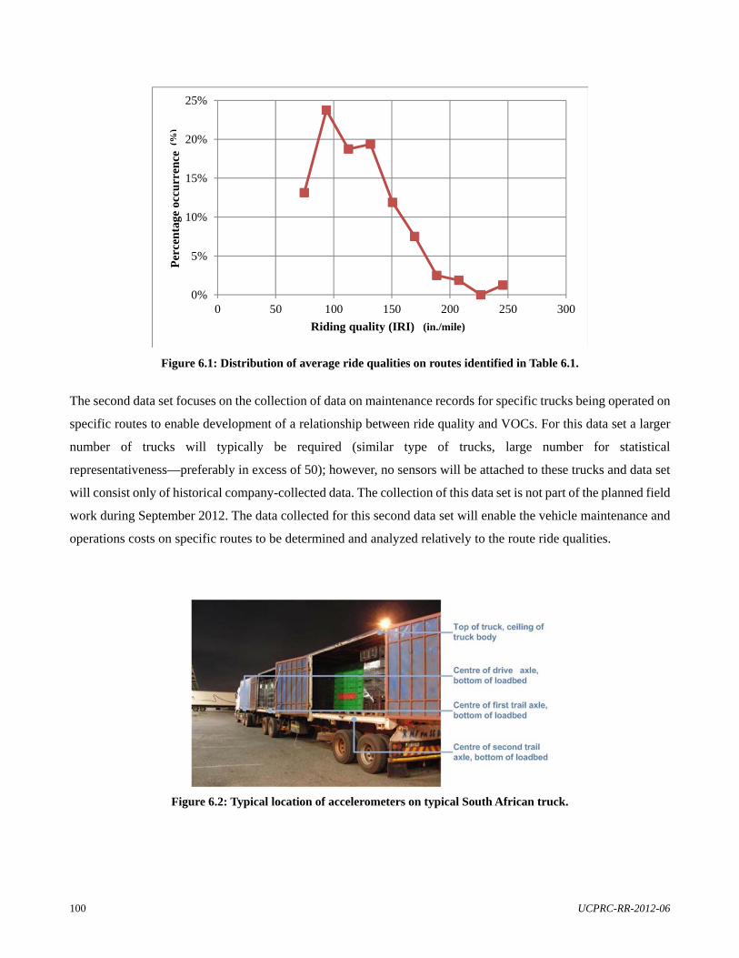
100 UCPRC-RR-2012-06
Figure 6.1: Distribution of average ride qualities on routes identified in Table 6.1.
The second data set focuses on the collection of data on maintenance records for specific trucks being operated on
specific routes to enable development of a relationship between ride quality and VOCs. For this data set a larger
number of trucks will typically be required (similar type of trucks, large number for statistical
representativeness—preferably in excess of 50); however, no sensors will be attached to these trucks and data set
will consist only of historical company-collected data. The collection of this data set is not part of the planned field
work during September 2012. The data collected for this second data set will enable the vehicle maintenance and
operations costs on specific routes to be determined and analyzed relatively to the route ride qualities.
Figure 6.2: Typical location of accelerometers on typical South African truck.
0%
5%
10%
15%
20%
25%
0 50 100 150 200 250 300
Per
cen
tage
occ
urr
ence
[%
]
Riding quality (IRI) [inch/mile](in./mile)
(%)
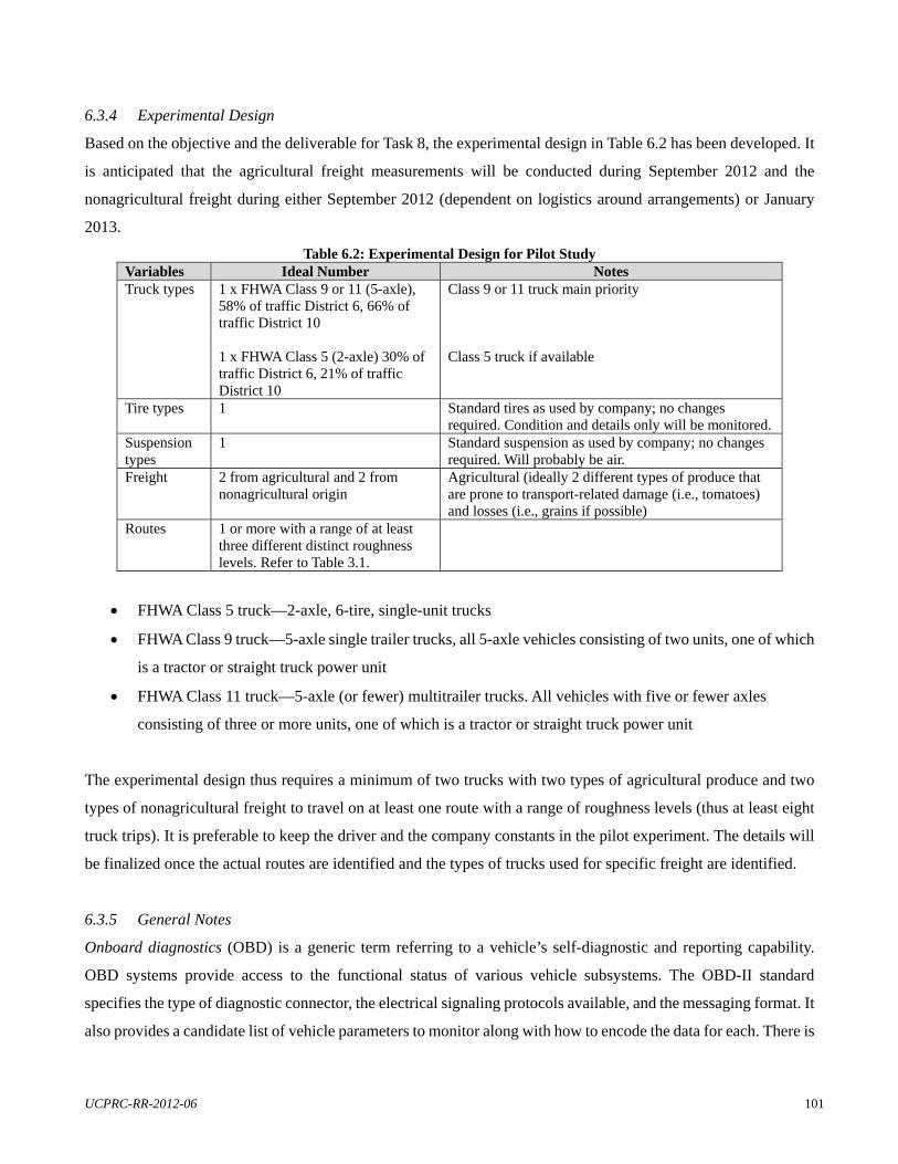
UCPRC-RR-2012-06 101
6.3.4 Experimental Design
Based on the objective and the deliverable for Task 8, the experimental design in Table 6.2 has been developed. It
is anticipated that the agricultural freight measurements will be conducted during September 2012 and the
nonagricultural freight during either September 2012 (dependent on logistics around arrangements) or January
2013.
Table 6.2: Experimental Design for Pilot Study Variables Ideal Number Notes Truck types 1 x FHWA Class 9 or 11 (5-axle),
58% of traffic District 6, 66% of traffic District 10 1 x FHWA Class 5 (2-axle) 30% of traffic District 6, 21% of traffic District 10
Class 9 or 11 truck main priority Class 5 truck if available
Tire types 1 Standard tires as used by company; no changes required. Condition and details only will be monitored.
Suspension types
1 Standard suspension as used by company; no changes required. Will probably be air.
Freight 2 from agricultural and 2 from nonagricultural origin
Agricultural (ideally 2 different types of produce that are prone to transport-related damage (i.e., tomatoes) and losses (i.e., grains if possible)
Routes 1 or more with a range of at least three different distinct roughness levels. Refer to Table 3.1.
FHWA Class 5 truck—2-axle, 6-tire, single-unit trucks
FHWA Class 9 truck—5-axle single trailer trucks, all 5-axle vehicles consisting of two units, one of which
is a tractor or straight truck power unit
FHWA Class 11 truck—5-axle (or fewer) multitrailer trucks. All vehicles with five or fewer axles
consisting of three or more units, one of which is a tractor or straight truck power unit
The experimental design thus requires a minimum of two trucks with two types of agricultural produce and two
types of nonagricultural freight to travel on at least one route with a range of roughness levels (thus at least eight
truck trips). It is preferable to keep the driver and the company constants in the pilot experiment. The details will
be finalized once the actual routes are identified and the types of trucks used for specific freight are identified.
6.3.5 General Notes
Onboard diagnostics (OBD) is a generic term referring to a vehicle’s self-diagnostic and reporting capability.
OBD systems provide access to the functional status of various vehicle subsystems. The OBD-II standard
specifies the type of diagnostic connector, the electrical signaling protocols available, and the messaging format. It
also provides a candidate list of vehicle parameters to monitor along with how to encode the data for each. There is

102 UCPRC-RR-2012-06
a pin in the connector that provides power for the scan tool from the vehicle battery, which eliminates the need to
connect a scan tool to a power source separately. Finally, the OBD-II standard provides an extensible list of
diagnostic trouble codes (DTCs). As a result of this standardization, a single device can query the onboard
computer(s) in any vehicle. Most manufacturers have made the OBD-II Data Link Connector the only one in the
vehicle, through which all systems are diagnosed and programmed (41).
6.4 Caltrans Decision
Based on the information presented in this report, as well as the discussions on the data and the analyses and
syntheses in Sections 5 and 6, it is recommended that the San Joaquin Valley be used as the pilot region for this
project.
The I-5, SR 58, and SR 99 routes are recommended as preferred routes for the pilot study. However, if vehicles
that travel on other, similar routes are the only vehicles available for the pilot study, their routes may be used in the
pilot analyses instead.

UCPRC-RR-2012-06 103
7 CONCLUSIONS AND RECOMMENDATIONS This section only contains the major conclusions and recommendations from this project to date. Section 6.2
provides a detailed overview of the information obtained from the project, and Section 6.3 contains details on the
anticipated field work for Task 8.
7.1 Conclusions
The following conclusions are drawn based on the information provided and discussed in this report:
Ample information exists to enable the objectives of this pilot study to be met through analyzing the V-PI
and logistics situation in a selected corridor in California.
The San Joaquin Valley corridor is a major production and transportation corridor in California and
well-suited to serve as pilot area for the purposes of the remainder of this project.
7.2 Recommendations
The following recommendations are made based on the information provided and discussed in this report:
The San Joaquin Valley should be targeted as the pilot study area for the purposes of the remaining tasks in
this pilot project.
The work anticipated for Tasks 7–12 should commence once this report has been accepted and approved
by the client.

104 UCPRC-RR-2012-06
UCPRC-RR-2012-06 105
8 REFERENCES 1. Gillespie, T.D. Fundamentals of Vehicle Dynamics. Warrendale, PA: Society for Automotive Engineers. 1992.
2. Sayers, M.W., Gillespie, T.D., and Paterson, W.D.O. Guidelines for Conducting and Calibrating Road
Roughness Measurements. World Bank Technical Paper Number 46. Washington, D.C.: World Bank, 1986.
3. ASTM. Terminology Related to Travelled Surface Characteristics (E 867). West Conshohocken, PA:
American Society for Testing and Materials,( 1996.
4. Hegmon, R.R. “Definition and Management of Pavement Surface Roughness.” Wear 57: 127–136 (1979).
5. McClean, J., and Ramsay, E. Interpretations of Road Profile-Roughness Data: Review and Research Needs.
ARRB Research Report 295. Melbourne, Australia: Australian Road Research Board, 1996.
6. MTO: Ontario’s Transportation Technology Transfer Digest 16,3.
http://www.mto.gov.on.ca/english/transtek/roadtalk/rt16-3/ (Accessed 2012.)
7. Sayers, M.W., Gillespie, T.D., and Queiroz, C.A.V. The International Road Roughness Experiment:
Establishing Correlation and a Calibration Standard for Measurements. World Bank Technical Paper
Number 45. Washington, D.C.: World Bank, 1986.
8. Structural Design of Flexible Pavements for Interurban and Rural Roads. Technical Recommendations for
Highways TRH4. Pretoria, South Africa: Committee of Land Transport Officials (COLTO), Department of
Transport, 1996.
9. Sayers, M.W., and Karamihas, S.M. The Little Book of Profiling. Ann Arbor: University of Michigan, 1998.
10. Sayers, M.W. “On the Calculation of International Roughness Index from Longitudinal Road Profile.” In
Pavement-Vehicle Interaction and Traffic Monitoring, pp. 1–12. Transportation Research Record 1501.
Washington, DC: Transportation Research Board, National Research Council, 1995.
11. Mann, A.V., McManus, A.M., and Holden, J.C. “Power Spectral Density Analysis of Road Profiles for Road
Defect Assessment.” Road and Transport Research 6,3: 36–47 (1997).
12. Sayers, M.W., and Karamihas, S.M. Interpretation of Road Roughness Profile Data.
FHWA-RD-96-101McLean, VA: Federal Highway Administration, 1996.
13. Papagiannakis, A.T., and Gujarathi, M.S. “Roughness Model Describing Heavy Vehicle-Pavement
Interaction.” In Pavement-Vehicle Interaction and Traffic Monitoring, pp. 50–59.. Transportation Research
Record 1501. Washington, DC: Transportation Research Board, National Research Council, 1995.
14. Huhtala, M. “The Effect of Wheel Loads on Pavements.” In Road Transport Technology 4: Proceedings of the
Fourth International Symposium on Heavy Vehicles and Dimensions. Ed. C.B. Winkler, pp. 235–241. Ann
Arbor: University of Michigan Transportation Research Institute, 1995.
15. ISO. Mechanical Vibration: Road Surface Profiles—Reporting of Measured Data. ISO 8608: 1995(E).
Geneva: International Organisation for Standardization, 1995.
106 UCPRC-RR-2012-06
16. ProVal. ProVAL Workshop: Pavement Profile Viewing and Analysis Software. TRB 2009. Washington DC.
www.roadprofile.com (Accessed 2009).
17. Caltrans. Caltrans Office of Truck Services. http://www.dot.ca.gov/hq/traffops/trucks/truckmap/ (Accessed
April 16, 2012).
18. FHWA. Traffic Monitoring Guide. http://www.fhwa.dot.gov/ohim/tmguide (Accessed June 4, 2012).
19. RITA. Commodity Flow Survey. State—California. Research and Innovative Technology Administration,
Bureau of Transportation Statistics, USA.
http://www.bts.gov/publications/commodity_flow_survey/2007/states/california/index.html# (Accessed June
4, 2012).
20. Lu, Q., Harvey, T., Lea, J., Quinley, R., Redo, D., and Avis, J. Truck Traffic Analysis Using Weigh-In-Motion
(WIM) Data in California. Berkeley: Institute of Transportation Studies, Pavement Research Center,
University of California, 2002.
21. Wang, F., Inman, R.F., Machemehl, R.B., Zhang, Z., and Walton, C.M. Study of Current Truck Configurations.
FHWA/TX-05/0-1862-1. Austin, TX: Center for Transportation Research, 2000, rev. 2004.
22. Simpson, Z., and Havenga, J.H. “National Land Freight Transport Activity.” In Eighth State of Logistics
Survey for South Africa, 2011, pp. 51–57. Pretoria, South Africa: Council for Scientific and Industrial
Research, 2012.
23. U.S. Department of Transportation, Research and Innovative Technology Administration, Bureau of
Transportation Statistics and U.S. Department of Commerce, U.S. Census Bureau, 2007 Economic Census:
Transportation Commodity Flow Survey, December 2009.
http://www.rita.dot.gov/bts/sites/rita.dot.gov.bts/files/publications/commodity_flow_survey/2007/states/calif
ornia/html/table_01a.html (June 12, 2012).
24. Cambridge Systematics. San Joaquin Valley Interregional Goods Movement Plan: Draft Truck Commodity
Flow Summary. Oakland, CA: Cambridge Systematics, 2012.
25. Sigala M., and Fischer, M. San Joaquin Valley Interregional Goods Movement Plan—Stakeholder Advisory
Committee Update on Progress. Fresno, CA: San Joaquin Valley Regional Planning Agencies, 2012.
www.sjvcogs.org/goods.html (Accessed March 15, 2012.)
26. Cambridge Systematics. San Joaquin Valley Interregional Goods Movement Plan: Existing Conditions
Assessment Technical Memorandum. Oakland, CA: Cambridge Systematics, 2012.
27. Tioga Group. Tomato Industry Profile: San Joaquin Valley Industry Profile. Moraga, CA: The Tioga Group,
2011.
28. Tioga Group. Dairy Industry Profile: San Joaquin Valley Industry Profile. Moraga, CA: The Tioga Group,
2012.

UCPRC-RR-2012-06 107
29. Goods Movement Action Plan. Business, Transportation, and Housing Agency; and California Environmental
Protection Agency, 2007.
30. Sandberg, U., Bergiers, A., Ejsmont, J.A., Goubert, L., Karlsson, R., and Zöller, M. “Road Surface Influence
on Tyre/Road Rolling Resistance.” Deliverable # 4 in MIRIAM SP 1. Swedish Road and Transport Research
Institute (VTI), 2011.
31. Tioga Group. California Inter-Regional Intermodal System (CIRIS) Implementation Plan. Prepared for San
Joaquin Council of Governments. Moraga, CA: The Tioga Group, 2006.
32. KOA Corporation. I-5/SR-99 Origin And Destination Truck Study. Monterey Park, CA: KOA Corporation
Planning and Engineering, 2009.
33. Steyn, W.J.vdM., Bean, W.L., and Monismith, C.L. “The Potential Costs of Bad Roads in South Africa.” In
The Fifth Annual State of the Logistics Survey for South Africa, CSIR BE, Pretoria, South Africa. Eds. Ittmann,
H., Havenga, J., and De Swart A., pp. 49–51. Pretoria, South Africa: Council for Scientific and Industrial
Research, 2009.
34. Steyn, W.J.vdM., and Bean, W.L. “Cost of Bad Roads to the Economy.” In The Sixth Annual State of the
Logistics Survey for South Africa, CSIR BE, Pretoria, South Africa. Eds. Ittmann, H., Havenga, J., and De
Swart A., pp. 24–30. Pretoria, South Africa: Council for Scientific and Industrial Research, 2010.
35. Steyn, W.J.vdM., and Bean, W.L. “The Potential Effects of Deteriorating Road Quality and Maintenance in
South Africa.” In The Seventh Annual State of the Logistics Survey for South Africa, CSIR BE, Pretoria, South
Africa. Eds. Ittmann, H., Havenga, J., and De Swart A., pp. 30–35. Pretoria, South Africa: Council for
Scientific and Industrial Research, 2011.
36. Steyn, W.J.vdM., Bean, W.L., Pretorius, C.J., and Van der Walt, G.L. The Potential Effects of Bad Roads on
Transported Cargo. Eighth State of Logistics Survey for South Africa, 2011. Ed. Viljoen, N., pp. 79–86.
Pretoria, South Africa: Council for Scientific and Industrial Research, 2012.
37. Garcia-Romeu-Martinez, M.A., Singh, S.P., and Cloquell-Ballester, V.A. “Measurement and Analysis of
Vibration Levels for Truck Transport in Spain as a Function of Payload, Suspension and Speed.” Packaging
Technology and Science 21: 439–451 (2008).
38. Barchi, G.L., Berardinelli, A., Guarnieri, A., Ragni, L., and Totaro Fila, C. “Damage to Loquats by
Vibration-Simulating Intra-State Transport.” Biosystems Engineering 82(3): 305–312 (2002).
39. Vursavus, K., and Ozguven, F. “Determining the Effects of Vibration Parameters and Packaging Method on
Mechanical Damage in Golden Delicious Apples.” Turkish Journal of Agriculture and Forestry 28: 311–320
(2004).
40. Singh, S.P., Joneson, E., Singh, J., and Grewal, G. “Dynamic Analysis of Less-Than-Truckload Shipments
and Test Method to Simulate This Environment.” Packaging and Technology Science 21: 453 – 466 (2008).
41. Wikipedia. OBDII technology. http://en.wikipedia.org/wiki/OBDII. (Accessed June 12, 2012.)

108 UCPRC-RR-2012-06
TECHNICAL APPENDICES
APPENDIX A: MINUTES OF PROJECT KICKOFF MEETING
A.1. Introduction
This appendix contains a copy of the minutes of the kickoff meeting held on 2 February 2012 in Sacramento,
California.
Division of Research and Innovation February 2, 2012
Office of Materials and Infrastructure
SPR Part 1 Special Study – DRAFT Contact List
Recorder – B. Nokes
Meeting Summary – Project Kickoff for SPR Part I Special Study: “Pilot Study Investigating the Interaction and
Effects for State Highway Pavements, Trucks, Freight, and Logistics”
The meeting Sign-in Sheet and Agenda are shown below. Discussions followed the meeting agenda. Handouts at
the meeting included: (1) names and contact information for project members (updated Contact List is included in
final page of this summary) and (2) project proposal/workplan. The meeting started at 10:00 am and adjourned at
11:35 am.
Discussions and follow-up actions are highlighted here.
Rose is the project lead contact at DOTP. Bill is the project lead contact at DRISI (task manager for this
task within for the UCPRC contract). Joe is the UCPRC contract manager in DRISI.
Wynand showed the webpage link to get copies of South Africa State of Logistics reports.
Wynand will email his MS PowerPoint file to DOTP/DRISI.
The location (region as opposed to a specific Caltrans District) for road profile and truck analysis and
truck instrumentation will be investigated and then decided by Task 6. Potential locations discussed
included the South Coast and Bay Area. South Coast (District 7) efforts and good sources of information
also include potential coordination with SCAG and UC Irvine, which are developing new models. Bay
Area (District 4) could provide linkages to more local sites (e.g., Port of Oakland, agricultural producers
in District 3) that may be better suited to this pilot study.
The type of freight (e.g., agriculture, electronics) suitable to focus on in this pilot study also will be
decided by Task 6.
The location and freight sector for instrumentation of trucks will be decided by the project team after
identifying road and vehicle inventory data, gathering other necessary information including
UCPRC-RR-2012-06 109
private-sector contacts, and completing technical discussions, which are expected to culminate in a
decision by June 2012.
The risk of not obtaining in-service trucks for instrumentation may be mitigated by starting now to (1)
identify contacts in various sectors (e.g., Caltrans and outside professional contacts, electronics/computer,
agribusiness associations, local farmers) and (2) investigate potential coordination of this task with related
UCPRC projects that may provide access to trucks.
Other potential Caltrans contacts to follow-up with who may be helpful for the project include (1) Joanne
McDermott (DOTP Freight Planning) to identify possible industry contacts for instrumentation of trucks
and (2) Sarah Chesebro (Transportation Systems Information, TSI, Travel Forecasting and Analysis
Office) and Doug MacIvor (TSI, Transportation/Freight Modeling & Data Branch). Alfredo suggested
potential contacts with the farming sector may be achieved through contact with UC Extension.
Jackie shared a sample of SPR Part I Annual Report form the DOTP submits to the FHWA. Wynand &
Louw offered to follow its format in their monthly project updates. Jackie will email the forms to all.
Communication and feedback were emphasized as priorities. Virtual meetings, e.g., using WebEx, will be
planned in the coming months to keep up project team communication and feedback. Austin is a resource
in DOTP to help set up WebEx meetings. Wynand and Louw can easily shift their schedules for WebEx
meetings so that the 9–10 hour time zone difference will not be a barrier to communications.
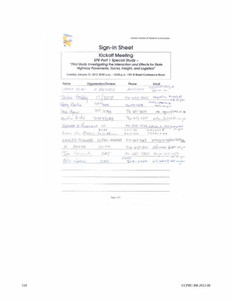
110 UCPRC-RR-2012-06

UCPRC-RR-2012-06 111