1

Freeway Segment Traffic State Estimation

Heterogeneous Data Sources and Uncertainty Quantification:

A Stochastic Three-Detector Approach

Wen DengXuesong Zhou

University of Utah

Prepared for INFORMS 2011

2

Needs for Traffic State Estimation

Sensor Data Traffic State Estimation Traffic Flow/Control Optimization

3

Motivating Questions• How to estimate freeway segment traffic

states from heterogeneous measurements?– Point mean speed– Bluetooth travel time records– Semi-continuous GPS data

Automatic Vehicle Identification Automatic Vehicle LocationLoop Detector Video Image Processing

Point Point-to-pointSemi-continuous path trajectory

Continuous path trajectory

4

Motivating Questions

• How much information is sufficient?– How to locate point sensors on a traffic segment?– How to locate Bluetooth reader locations?– How much AVI/GPS market penetration rate is

sufficient?

5

Existing Method 1: Kalman Filtering

• Eulerian sensing framework– Muñoz et al., 2003; Sun et al., 2003; Sumalee et

al., 2011– Linear measurement equations to incorporate

flow and speed data from point detectors

• Extended Kalman filter framework– second-order traffic flow model– Wang and Papageorgiou (2005)

6

Existing Method 2: Cell Transmission Model

0 10 20 30 40 50 60 70 80 90 100 110 120 1300

200400600800

100012001400160018002000

Density (vhc/ml/lane)

Flo

w v

olu

e (v

hc/

hou

r/la

ne)

Cell inflow inequalityqi,j(t) = Min { vfree ki,j(t) , qmax i,j(t) , w (kjam - ki,j(t)) Δ x }

Switching-mode model (SMM)set of piecewise linear equations

qi,j(t) = [vfree ki,j(t) ] + [vfree ki,j(t) ]

7

Existing Method 3: Lagrangian sensing

• Nanthawichit et al., 2003; Work et al., 2010; Herrera and Bayen, 2010

• Establish linear measurement equations • Utilize semi-continuous samples from moving

observers or probes

8

Existing Method 4: Interpolation method

• Treiber and Helbing, 2002– “kernel function” that builds the state equation for

forward and backward waves– Linear state equation through a speed

measurement-based weighting scheme

Figure Source: Treiber and Helbing, 2002

9

Challenge No.1

• 1. Unified measurement equations to incorporate– Point, point-to-point and semi-continuous data

10

Our New Perspective• Dr. Newell’s three-detector model provides a

unified framework• N(t,x)=Min {Nupstream(t-BWTT)+Kjam*distance, Ndownstream(t-FFTT)}

Time axis

( )( )

b

length bBWTT b

w

( )( )

f

length aFFTT a

v

Time t-1

Spac

e axi

s

Link b

Link a

A(b,t-1)

D(b,t-BWTT(b)-1)

11

1: From Point Sensor Data to Boundary N-curves

• Cell density and flow are all functions of cumulative flow counts

12

2: From Bluetooth Travel Time to Boundary N-curves

• Downstream and upstream N-Curves between two time stamps are connected

13

3: From to GPS Trajectory Data to Boundary N-curves

• Under FIFO conditions, GPS probe vehicle keeps the same N-Curve number (say m)

m

m

mm

m

14

4: From Boundary N-curves to Everything inside S

pac

e ax

is

Cumulative flow count n(t,x) space

Time

t0 t3

t t+ΔT

x+ΔX

xN(x,t) N(x,t+ΔT)

N(x+ΔX,t) N(x+ΔX,t+ΔT)

length xD t

w

length x XD t

w

f

xA t

v

f

x XA t

v

15

Challenge No. 2

• All sensors have errors error propagation

Surveillance Type Data Quality

Point Detectors High accuracy and relatively low reliability

AutomaticVehicle Identification

Accuracy depends on market penetration level of tagged vehicles

Mobile GPS location sensors Accuracy depends on market penetration level of probe vehicles

Trajectory data from video image processing

Accuracy depends on machine vision algorithms

16

The Question We have to Answer

• Under error-free conditions, Newell’s model provides a good traffic state description tool

N(t,x) =Min {Nupstream(*), Ndownstream(*)}

• With measurement errors• What are the mean and variance of

– Min {Nupstream(*)+eu, Ndownstream(*) +ed}

17

Quick Review: Probit Model and Clark’s Approximation

• Probit model (discrete choice model for min of two alternatives’ random utilities )– U = min (U1+e1, U2+e2)– Route choice application

• Clark’s approximation

minimization of two random variables can be approximated by a third random

variables

18

Proposed Stochastic 3-Detector Model

19

Discussion 1: Consistency CheckingWhen Uncertainties of boundary values are 0, the stochastic 3-detector model reduces to deterministic 3-detertor model

20

Discussion 2: Weights under Different Traffic Conditions

21

Discussion 3: Quantify Uncertainty of Inside-Traffic-State Estimates

• Variance or trace of estimates determine the value of information

1 1T

2 2

3 3

E(e e )

Trace(ee )= E(e e )

E(e e )

22

Stochastic Boundary

A priori Estimation Variance-Covariance Matrix

A priori Cumulative Vehicle Count Vector Estimation

N

P

1

2A posterior estimation of

Variance-Covariance Matrix

A posterior estimation ofCumulative Vehicle Count Vector

N

P

4

5

Linear Measurement Equations

Y HN R 3

Cell Based Flow and DensityEstimation

Cell Based Flow and DensityUncertainty Quantification

12

13

AVI Measurements

Travel Times

Additional Point Sensor

Measurements

Vehicle Counts

Occupancy

GPS Measurements

Vehicle Number

Speed

7. Heterogeneous Data Sources

Stochastic Three Detector Model

Newell’s Simplified Kinematic Wave TheoryMinimization Equation

Probit Model and Clark’s ApproximationSolution to a Minimization Equation

8

9 Boundary N Mapping Matrix H

Measurement Error Variance Covariance

R

Point Sensor Sampling Time Interval

AVI Market Penetration Rate

GPS Market Penetration Rate

10

11

6. Parameters

23

Numerical Example

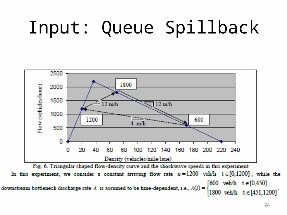
24

Input: Queue Spillback

25

Ground truth Arrive-departure Curves

26

Estimated Density Profile

27

Estimated Uncertainty profileBefore

After

28

Impact of Additional Sensors

29

Possible (Un-captured) Modeling Errors

• Upper plot: original NGSIM vehicle trajectory data• Lower plot: reconstructed vehicle trajectory based on flow count measurements

1. Stochastic free-flow speed, 2. Stochastic backward wave speed;3. Heterogeneous driving behavior

30

Conclusions

• Proposed stochastic 3-detertor Model– Estimate freeway segment traffic states from

heterogeneous measurements– Quantify the degree of estimation uncertainty and

value of information, under different sensor deployment plans