Reports of the Department of Geodetic Science

Report No. 195

FREE GEOMETRIC ADJUSTMENT OFTHE SECOR EQUATORIAL NETWORK

(Solution SECOR-27) crs a S

by 0C

Ivan I. Mueller, M. Kumar and Tomas Soler -

o, wC1

Prepared for 0 0o

National Aeronautics and Space Administration oS tdWashington, D. C.

Contract No. NGR 36-008-093OSURF Project No. 2514 )

The Ohio State UniversityResearch Foundation .

Columbus, Ohio 43212

February, 1973

Reports of the Department of Geodetic Science

Report No. 195

FREE GEOMETRIC ADJUSTMENT OF

THE SECOR EQUATORIAL NETWORK

(Solution SECOR-27)

by

Ivan I. Mueller, M. Kumar and Tomas Soler

Prepared for

National Aeronautics and Space AdministrationWashington, D. C.

Contract No. NGR 36-008-093OSUF Projet No. 25F14

The Ohio State UniversityResearch Foundation

Columbus, Ohio 43212

February, 1973

PREFACE AND ACKNOWLEDGEMENT

This project is under the supervision of Ivan I. Mueller, Professor

of the Department of Geodetic Science at The Ohio State University and is

under the technical direction of James P. Murphy, Special Programs,

Code ES, NASA Headquarters, Washington, D.C. The contract is admin-

istered by the Office of University Affairs, NASA, Washington, D.C., 20546.

The authors wish to express their appreciation to the Defense Mapping

Agency (Topographic Center) for the SECOR data, and for other helpful in-

formation related to the analysis of the data.

ii

TABLE OF CONTENTS

Page No.

PREFACE AND ACKNOWLEDGEMENTS ii

TABLE OF CONTENTS iii

1. INTRODUCTION 1

2. DATA 3

2.1 Terrestrial Data 32.2 Satellite Observational Data and Its Handling 3

3. THEORETICAL BACKGROUND 14

3.1 The Mathematical Model 143.2 Normal Equations 163.3 Reduced Normal Equations 163.4 Constraints Contributions to the Normal Equations 17

3.41 Relative Position Constraints 193.42 Height Constraints 213.43 Directional Constraints 213.44 Inner Constraints (Free Adjustment) 23

4. THE SOLUTION 26

5. COMPARISON WITH OTHER SOLUTIONS 36

6. CONCLUSIONS 44

REFERENCES 45

LIST OF TABLES

TABLE 2.1-1 Survey Information of Observations Stations 4TABLE 2.1-2 Geodetic Datums 6TABLE 2.1-3 Relative Position Constraints 7TABLE 2.1-4 Geoidal Undulations and Heights used in Constraints 8TABLE 2.1-5 Direction Constraints between BC-4 Stations 9TABLE 2.2-1 Summary of SECOR Observations by Quadrangle 12TABLE 4-1 General Information on the SECOR-27 Geometric 26

AdjustmentTABLE 4-2 Cartesian and Geodetic Coordinates (Solution SECOR-27) 27TABLE 5-1 Transformation: NWL 9D-SECOR-27 37TABLE 5-2 Transformation: SAO III - SECOR-27 39TABLE 5-3 Transformation: WN14 - SECOR-27 41

iii

1. INTRODUCTION

The basic purpose of this experiment is to compute reduced normal

equations from the observational data of the SECOR Equatorial Network

(Fig. 1) obtained from DMA/Topographic Center, D/Geodesy, Geosciences

Div., Washington, D.C. These reduced normal equations are to be combined

with reduced normal equations of other satellite networks of the National

Geodetic Satellite Program to provide station coordinates from a single

least square adjustment.

An individual SECOR solution was also obtained and is presented in

this report, using direction constraints computed from BC-4 optical data

from stations collocated with SECOR stations. Due to the critical configur-

ation present in the range observations [Blaha, 1971], weighted height con-

straints were also applied in order to break the near coplanarity of the

observing stations.

Details of the SECOR network, including instrumentation, historical

background, etc., are given in Rutscheid [197]].

1

5754

20 9

01 5713

911 5739 592 448 31

5972 5712 595572

t r 5733 5934

5735 0 5736 5738

05732

Fig. 1 SECOR Equatorial Network.

2. DATA

2.1 Terrestrial Data

Terrestrial data including survey coordinates and mean sea level

heights of stations, instrument type used, etc., are given in Table 2.1-1,

together with a list of geodetic datums involved (Table 2.1-2).

These survey coordinates-provide the necessary relative position con-

straints between 13 SECOR stations and collocated BC-4 stations and in ad-

dition relative position constraint between two SECOR stations [Mueller,

et al., 1973]. Constraints used in this experiment are given in Tables

2.1-3, 2.1-4 and 2.1-5. Geoidal undulations (Table 2.1-4) were computed

by using formula and constants as given in [Rapp, 1973].

2.2 Satellite Observational Data and Its Handling

The magnetic tape containing SECOR data, obtained from.the De-

fense Mapping Agency, created on the UNIVAC 1108 EXEC 8

System was translated to a 9-track BCD tape for use on the IBM 360 computer.

For checking purposes, a printout of the ranges with the first and

second differences was obtained. No major blunders (besides some duplica-

tion of a few observations) were detected.

Corrections to the ranges were applied according to Figure 2.2-1 and

a new data set was generated for all the simultaneous observations from four

stations. This data in a new format (OSUGOP [Reilly, et al., 1972]) was

transferred to a tape. A summary of these observations by quadrangle is

given in Table 2.2-1.

3

Table 2.1-1

SURVEY INFORMATION OF OBSERVATION STATIONS--------- ---------- ----------------------------------------------------------------

S T A T 1 0 N I UATuMI S U R V E Y C 0 0 R 0 I N A T E S2 I SL I INSTR. 4 INSTR. ISOURCEII----- I..I -------------------------------------- I I HEIGHTII

I C N A M I CODE I LATITUDE LONGITUDE IELL. H(M) I (M) I (M) I TYPE I CODES-- -- - -------- -- - -------------------------- ----------- -- ----

I I I I I I I I I5001 I HERNDON 29 380 59' 37':697 282o

40' 16'.705 129.0 127.80 9.39 SECOR I I I5201 MOSES LAKE 29 47 11 5.916 240 39 50.463 358.0 368.92 2.00 SECOR I I I54"0 SAN ISLAND 27 28 12 32.061 182 37 49.531 6.0 6.10 4.13 SECOR 25648 FORT STEWART 29 31 55 18.405 278 26 0.260 34.0 27.80 3.90 SECOR I15712 PARAMARIBO 41 5 26 59.817 304 47 44.990 I 12.0 21.50 1 4.93 I SECOR I 1

5713 I TERCEIRA I 17 I 38 45 56.725 332 54 21.064 56.0 56.00 4.25 SECOR 1 I5715 DAKAR 50 I 14 44 41.008 342 30 52.935 27.0 27.30 4.42 SECOR I 15717 FORT LAMY 1 I 12 7 49.300 15 2 6.148 I 320.0 298.50 4.83 SECOR I 15720 ADIS AEA8A I 1 8 46 9.479 38 59 49.196 I 1681.0 I 1889.40 1 4.29 I SECOR I 1 I5721 MASHHAD 16 36 14 30.404 59 37 40.105 I 962.0 I 994.40 I 4.35 I SECOR I 1

I I I I I II I I I I I I I5722 I IEGO GARCIA I * I - 7 20 57.440 72 28 31.570 * 6.10 1 4.60 I SECOR 2 15723 IHIANG MAI * I 18 47 99 00 * I 310.80 I SECOR I 15726 I AOAtANGA 26 1 6 55 26.213 122 4 3.558 1 14.0 13.30 4.83 SECOR 257:0 I AKE ISLAND 49 I 19 17 24.100 166 36 41.206 I 8.0 I8.10 4.29 SECOR I5732 AGO PAGO I I * a I * I * I * I SECOR

57;3 igHRISTMAS ISLAND I 12 I 2 0 35.622 202 35 21.962 4.0 I 3.50 1 2.29 SECOR I5724 HEzYA 29 1 52 42 54.894 174 7 37.870 I -7.0 I 39.30 1.50 1 SECOR I 1 I5735 ATAL 41 I - 5 54 56.253 324 49 57.605 I 66.0 39.40 * I SECOR I 15736 SCENSION ISLAND 5 I - 7 58 15.220 345 35 32.365 74.0 74.00 4.32 SECOR I 15739 ERCEIRA 17 38 45 36.311 332 54 19.686 I 56.0 56.10 I 4.25 I SECOR I 1

I I I I I I I I I57-4 I TANIA I 16 I 37 26 40.831 15 2 44.955 I -4.0 11.80 4.17 SECOR 15907 W RTHINGTON I * * * I I SECOR I5911 e R:AUDA * I * I I I SECOR5912 P NAMA I a I I * I SECOR5914 P ERTO RICO I * I * * * I I * I SECOR i i

5915 IA STIN I a I a ** I * I SECOR I5923 2 CPRUS I * a I * f * * I SECOR I5924 iR TA * I * I * SECOR I5925 IR EERTS FIELD I* I * I * I I SECOR593C IS NGAPORE I * I * I * * I SECOR

SI I I I II 1 4 I I I II I I I

Table 2.1-1 (Cont'd)

SURVEY INFORMATION OF OBSERVATION STATIONS

I S T A T I 0 N I DATUMI S U R V E Y C 0 0 R D I N A T E S 2 I MSL 3 I INSTR. 1 I'STR. ISOURCEIS I ------------------------------------ I I HEIGHT 4

I I 5I NO I N A I CODE I LATITUDE LONGITUDE IELL. H(I) I (M) I (M) I TYPE I CCLE I

I I I I I I I I I I5931 I HONG KONG I * I * * * I * I * SECOR

S5933 ) DARWIN * I * * I I * j I SECOR5934 I MAUS I * I * * * I * I * I SECOR5935 I GUAM I * " * * I * I * I SEC'JR I5937 I PALAU I * * * I * * SECOR

I I I I I I I I I i5938 I GUADALCANAL I * * * * * * I SECOR5941 1 MAUI I * I I * * * I SECOR

I 6003 1 MOSES LAKE I 29 I 47 11 7.132 240 39 48.118 I 356.0 I 368.7,t 1.50 I EC-4A I 16004 I SHEMYA I 29 52 42 54.890 174 7 37.870 t -9.0 I 36.80 I 1.50 1 BC-4 I 16007 I TERCEIRA I 17 I 38 45 36.725 332 54 21.064 ( 53.0 5 5.30 1.49 B C-4 1

n 6008 i PARAMARILO I 41 I 5 26 55.325 304 47 42.832 I 8.7 I 10.36 I 1.49 I BC-4 i I6012 I WAKE ISLAND I I 49 I 19 17 23.227 166 36 39.7z0 I 4.0 I 3.50 1.50 I C-4 I 16015 1 MASHHAD I16 I Zo 14 29.527 59 37 42.729 I 959.0 I 991.00 1 1.50 E C-4 I 16016 I CATANIA I 16 1 37 26 42.628 15 2 47.308 -7.0 1 9.24 I 1.50 5 EC-4A I 16042 I ADDIS ABABA I 1 8 46 8.501 38 59 49.164 I 1878.0 1886.46 I 1.52 I SC-4 I 1

6047 I 2A:4XANGA 26 1 6 55 26.132 122 4 4.538 I 9.0 1 9.39 I 1.50 EBC-4 I 26055 ASCEiNSION ISLANI0 5 - 7 58 .6.634 345 35 32.764 1 71.0 I 70.94 1 1.50 I BC-4 I 16059 CHRISTMAS ISLAND I 12 i 2 0 35.622 202 35 21.962 1 3.0 2.75 I 1.50 1 BC-4A 1 I606$ I DAKAR I 50 1 14 44 44.22b 342 30 55.594 I 26.0 I 26.30 I 1.50 I BC-4A I 16067 INATAL 1 41 1-5 55 37.414 324 50 6.200 66.7 I 40.63 I * BC-4A I 1

- - - - I I I I I I I

* Data Not Available1 Refer to Table 2.1-22 Geodetic Coordinates of the Instrumental Reference Point (Optical/Electronic Center,

etc.) on the Local Geodetic Datum3 Mean Sea Level Height of the Instrumental Reference Point4 Height of Instrumental Reference Point above Survey Monument5 Source Code:

1 -- (CSC, 1971)2 --. (CSC, 1972/73)

Note: Zero in the last digit may indicate that the digit is unknown."N.

Table 2.1-2

GEODETIC DATUMS

- - T ---------- ----------------------

iOD! DATUM ELLIPSOID ORIGIN LATITUDE LCNGITUDE(E)--------------- ----- --------------- --------------- -- ------ -----------------

1 A INDAN (ETHIOPIA) CLARKE 1880 STATION Z5 ADINDAN~ 22010' 07110 31029' 21"608

5 A CENSION IS 1958 INTERN;ATIONAL MEAN OF 3 STATIONS -07 57 345 37

12 CHIRISTMAS IS ASTRO 1967 INTERNATIONAL SAT.TRI.STA. 059 RM3 02 00 35.91 202 35 21.82

16 ERCPEAN INTERNATIONAL HELMERT TOWER 52 22 51.45 13 03 58,74

17 GfACICSA IS (AZORES) INTERNATIONAL SW BASE 39 03 54.934 331 57 36.,118

26 LLZON 1911(PHILIPPINES) CLARKE 1866 FALANCAN 13 33 41.000 121 52 03.000

27 MIDWAY ASTRO 1961 INTERNATIONAL MIDWAY ASTRO 1961 28 11 34.50 182 36 24,,28

29 NORTH AMERICAN 1927 CLARKE 1866 MEADES RANCH 39 13 26.686 261 27 29..494

41 SOUTH AMERICAN 1969 S. 19RICAN 1969 CHUA -19 45 41.653 311 53 55.936

49 WAKE IS ASTRO 1952 INTERNATIONAL ASTRO 1952 19 17 19.991 166 3.8 46.294

50 YO ASTRO 1967 (DAKAR) CLARKE 1880 YOF ASTRO 1967 14 44 41.62 342 30 52.98

- ---- - ----------------------------

Table 2.1-3

RELATIVE POSITION CONSTRAINTS

I RELATIVE COORDINATES (METERS) IWEIGHTSISTATIONS I-----------I------------------------

SAu I Av I Aw It 1/ "2 )l,,,,,,-------------------------------

5201-6003 I 29.55 I -48.21 I -25.52 1.00 I

5712-6008 I 48.95 I 45.97 I 137.68 I1.00

5713-5739 I 8.05 I 33.26 9.95 I 20.00 I

5713-6007 1 2.08 I -1.06 I .1.88 1.00

5715-6063 I 1.05 I -83.72 I -95.45 I 1.00

5720-6042 1 -1.87 I -0.26 30.16 I 1.00

5721-6015 1 49.67 1 -44.84 23.59 1 1.00

5726-6047 I 30.82 24.81 3.07 1 1.00

5730-6012 1 -4.69 I -41.68 1 26.66 1 1.00

5733-6059 I -0.92 I -0.38 0.04 1 1.00

5734-6004 I -1.20 1 0.12 1 1.59 1 1.00

5735-6067 f -46.20 I -290.84 1257.74 I 1.00 1

5736-6055 I 5.82 I -13.48 42.60 1 1.00 1

5744-6016 49.84 1 -46.49 1 -42.16 I 1.00 1

SOURCE: DEFENSE MAPPING AGENCY TOPOGRAPHIC CENTER

1 APPLIED EQUALLY TO ALL THREE RELATIVE COORDINATES IN M-2 UNIT

7

Table 2.1-4

GEOIDAL UNDULATIONS AND HEIGHTS USED IN THE CONSTRAINTS

S T A T I 0 N I NREF I HCONSTR 21 0 II----------- ------------ I oNsrR

I No I N A M E I ( M ( M I (M).-- ---------------------------------------------

5001 I HERNDON 1 -36.87 1 69.67 1 6.0 15201 1 MOSES LAKE -17.65 341.99 I 4,0 I5410 I MIDWAY ISLANDS I - 4.13 i 6.72 1 .05648 1 FORT STEWART -35.07 I -29.10 I 2.5 I5712 I PARAMARIBO 1 -28.31 -40.09 I 4.0 I5713 TERCEIPA I 54.00 82.80 4.0 15715 DAKAR 27.20 I 20.91 4.0 I

5717 I FORT LAMY I 10.35 1 279.97 I 6.0 I5720 I ADDIS APABA - 5.78 . 1861.35 6.05721 MASNIHAD 1 -20.67 962.23 I 4.05722 1 DIEG GARCIA -73.64 1 -79.68 I 8.05723 I CHIANG MAI I -40.39 I 269.90 I 8.0 (5726 I ZAM6OANGA I 62.16 1 79.76 I 8.0

I 5730 I WAKE ISLAND I 13.75 I 28.88 I 8.0

5732 I PAGO PAGO I 27.35 I 35.16 I 6.05733 1 CHRISTMAS ISLAND 1 16.07 I 18.52 I 8.0 I.5734 I SHFMYA 1 6.22 I 48.36 I 8.05735 1 NATAL I -12.03 1 -9.55 1 6.05736 I ASCENSION ISLAND I 16.26 53.57 I 8.05739 I TERCEIRA 1 54.00 82.90 1 4.05744 I CATANIA I 37.43 I 26.13 I 4.0

5907 I WORTHINGTON I -28.11 I 437.93 I 2.55911 1 BERMUCA I -43.44 1 -47.06 8.05012 I PANAMA 6.16 I -11.73 I 6.05914 I PUERTO RICO I -50.08 I -14.72 6.05915 I AUSTIN I -26.32 I 162.18 I 2.55023 I CYPRUS I 24.64 I 168.92 8.0 15924 I ROTA 1 54.48 I 40.16 6.0 1

5925 I ROBERTS FIELD I 33.75 1 10.77 6.0 15930 SI SNGAPORE I 8.28 I 13.85 I 6.0 15o31 HONG KONG I 2.32 I 167.12 I 6.0 I5933 I DARWIN I 50.66 I 69.31 I 8.0 I5934 I MANUS I 74.75 I 86.77 1 8.0 I5935 GUAM I 48.15 1 92.63 I 8.05937 I PALAU 1 69.93 I 145.94 I 8.0 I

5938 I GUADALCANAL I 59.97 I 76.57 I 8.0 15941 I MAUI 1 2.05 1 34.51 I 8.0

----------------------------------------

1. From [Rapp, 1973]2. HCONSTR = MSL+NREF+,6N, where LN is a correction term for the dif-

ferences of position and size of the ellipsoids used [Mueller et al., 197313. Used in Computing the Weights of the Height Constraints

8

Table 2.1-5

DIRECTION CONSTRAINTS BETWEEN BC-4 STATIONS

Station-Station a a a

6003- 6004 -67? 598 1.'4 -4.994 11'4

6003- 6008 166.052 0.8 34.380 0.4

6004- 6047 -95.629 1.1 40. 651 1.1

6007- 6008 74.620 1.4 47. 803 1.4

6007- 6055 -157.541 1.1 69.401 1.1

6015- 6042 168.292 1.4 49.890 1.4

6015- 6047 -8.781 1.2 26.323 1.2

6016- 6042 -90.094 1.2 47.462 1.2

6016- 6055 112.934 0.9 56.487 0.9

For the definition of the angular components a and $ see section 3.43.These angles are based on station coordinates computed from theOSU WN14 solution [Mueller et al., 1973].

9

UNIVAC 1108 RawDataTape

SECOR I Robs = observed range measurement

IBM (9 track) BCDTransla- C HF' CF = observed frequency channel

tin HF LF cal-ibration correction (highand low frequency)

Raw data DI-DC.= given ionospheric correction forPrint out each range

A ,A ; AHF ,ALF given ambiguities

Ionospheric i 1 2 2 (initial and new sets)Correction

ARION RION = -0.7125 [(DI-IC) + A F + A2F + (CLF CHF)]

biguitiesShigh fre-

CalibrationCorrection(high frequency)

CHF

AS = .98 RobsAS 10

Corrected RRION HF HF

Range RI = Robs + + Ai A2 + CHF + ASRI

Fig. 2.2-1 Scheme of SECOR preprocessing procedure at OSU.

10

SECOR II

OSUGOPGeometricmode)ta.(ui viwi)at.(u.,v.,w.)

sin a = sins sing + coss cos(h G + X) coso. (See Fig. 2.2-2)Compute§atellite *,x station coordinatesaltitude "a"

hG,6 topocentric Greenwich hour angle and declination

ki(l - e- Robs)TROPO =

sin a + k2 cos a

Tropospheric whereCorrection k, = 2.7

"TROPO" k2 = 0.0236

Z = 1./7000.a = elevation angle

Final r = R - TROPOCorrected IRange

r I Print out I(OSUGOP forma )

FSECOR(OSUGOPformat

Fig. 2.2-1 continued

11

Satellite Qj (u3, v , wj)

w

St ion Pi (u ,W) -u

Greenwich /Mean v

Meridian

U

V -V t

tan (3600 - ho) = -tan hG -Uj -u t

V I -Vj V I

tan hG - tan X =-Uj -Ui u

wj -w I Wi

sin f - tanc =ri Iu + v2

sin a = sin f sin <p + cos f cos (h + X) cos (p

Figure 2.2-2

12

Table 2.2-1

SUMMARY OF SECOR OBSERVATIONS BY QUADRANGLE

Quad No. of Quad No. ofStations Involved Observations Stations Involved Observations

5001-5907-5648-5911 432 5726-5930-5933-5934 6445911-5001-5648-5914 168 5726-5933-5934-5935 8085911-5907-5915-5912 1008 5931-5726-5934-5935 11445911-5915-5912-5712 92 5935-5726-5934-5730 20485911-5907-5912-5712 260 5935-5726-5934-5937 12645911-5915-5912-5712 228 5730-5935-5934-5938 22165911-5912-5712-5713 684 5730-5935-5938-5732 13805713-5911-5712-5715 1220 5730-5938-5732-5733 7565715-5713 5712-5735 548 5730-5732-5733-5411 7525715-5739-5712-5735 288 5730-5733-5411-5410 648

5715-5712-5735-5736 660 5730-5733-5411-5734 5085715-5735-5736-5717 640 5734-5410-5411-5201 3125715-5736-5717-5744 28 5734-5730-5411-5201 2645739-5715-5717-5744 3845715-5736-5717-5744 4645744-5715-5717-5923 8685744-5715-5717-5924 8045744-5715-5717-5925 6125923-5744-5717-5720 12365923-5717-5720-5721 772

5744-5717-5720-5721 205721-5923-5720-5722 7525721-5720-5722-5723 2965923-5721-5722-5723 365723-5721-5722-5930 4605723-5722-5930-5931 5885722-5723-5930-5726 685931-5723-5930-5726 7685931-5930-5726-5933 10645723-5930-5726-5933 652

13

3. THEORETICAL BACKGROUND

3.1 The Mathematical Model

In the range observations mode each participating station Pj at an

event [E ,Qj I t ] observes the length of the distance (PIQ ) i.e., the topo-

centric range r t j from ground station P, to satellite position Qj (See

Fig. 2.2-2).

Let (us, v i , w 1 ) be the Cartesian coordinates of P, and (uS,v ,w,)

of QS, with respect to an average terrestrial (tied to the solid earth) co-

ordinate system defined by:

a) w - axis is directed toward the average north terres-

trial pole as defined by the International Polar

Motion Service (IPMS), commonly known as the

Conventional International Origin (CIO).

b) u-w plane parallel to the mean Greenwich astronomic

meridian as defined by the Bureau International de

1'Heure (BIH).

Thus the mathematical model can be written as

r, -Wi) 3.1-1

or

Fj = [(uS-u 1 )2 + (vj-vI)2 + (wj-w) 2 ] -r = 0 3.1-2

Thus in order to tie the satellite position points to the system only

three known stations observing simultaneously are necessary and sufficient

although we will not have redundant information. For redundant information

at least four stations observing simultaneously are necessary, provided their

configuration is not a degenerized one [Blaha, 1971a, Tsimis, 1973].

The expression for the linearized mathematical model as F is known

takes -theorm:

AX+ BV + W = 0

14

where the design matrix B is a negative unit matrix and the design matrix

A is formed by submatrices of the form:

Aj = A a., -a,

where

a U u tV -V - W

and r'J is computed from 3.1-1 using the initial approximate values for

the station. and satellite coordinates, the latest coordinates resulting from

a preliminary least squares adjustment (for each event j) with the observ-

ing stations held fixed. [Krakiwsky and Pope, 1967].

The unknown vector X is made up of subvectors

Xj

where

du[dv

anddu,

X, ldv /dw

The misclosure vector W is formed by the individual differences

WIj = ro (computed) - r, b (observed)

The residual vector V is composed of the individual residuals vil

(in meters) corresponding to the observed ranges rl . Giving consideration

to the characteristics of the design matrices, the final matrix equation for

the linearized model can be written as:

AX-V + W= O

or

AX+ W = V

15

3.2 The Normal Equations

The variation function for the range adjustment is similar to the

optical case, namely,

= V'PV + X'PxX - 2K' (AX - V + W) 3.3-1

where

V is the vector of residuals corresponding to the range observations

X is the vector of corrections to the preliminary ground and satel-

lite positions*

P is the weight matrix for the ranges

Px is the weight matrix for the ground and satellite positions

K is the vector of correlates

The differentiation of equation 3.2-1 for the minimum condition

results in the following expanded form of the normal equations:

-PX 0 A' X 0

0 -P -I + = 0 3.2-2

A -I 0 K W

After the elimination of the correlates and residuals, andt the expansion.of

the A and P matrices the following expression results:

Us=

Eal jpi a, j +P -a, iIpi X I I P L---- --I +.. . - ----------- = 0I U

-a Pi ai 1a, p ai. 1 +Pl 1J -Xa, pi .V

3.3 Reduced Normal Equations for Range Observations

The general form of the reduced normal equations after the elimina-

tion of Xj (corrections to the preliminary coordinates of the satellite position)

can be formulated as

NX+ U= 0

* Satellite positions will be considered "nuisance" parameters and there-fore eliminated from the solution.

16

where the 3 x 3 blocks in N are now computed using P,=0 [Mueller, 1968]:

Nkk = Ea , pl. akz - Za .pkaki [Zap 1.,ai.,]-akjpkjaj

3x3 .i

and the vector of constant terms having the form:

Uk -Z akl Pk Vkj

where

vk J = residual of any observed range from a particu-

lar station (resulting from a preliminary least

squares adjustment of any simultaneous event

with the stations held fixed).

pil = weight of any observed range r 1,

k, 1 denotes particular ground stations

j denotes particular simultaneous event

i denotes any ground station participating in an

event

Z is the summation over all ground stations in-

volved in event j.

L is the summation over all events observed by

ground station k and/or 1.

3.4 Constraint's Contributions to the Normal Equations

Two alternative definitions exist for the term "constraints". The ab-

solute constraints represent certain conditions which have to be fulfilled ex-

actly and with no uncertainties and the relative constraints (or weighted

constraints) which have the same characteristics as the observations.

In general the contribution of the functional constraint equations

G(X, Lc) = 0

17

to the normal equations can be found bordering the normal equation matrix

N,_1 Cn X, Un-1+ =0

C, -PI -Kcn W.-L- " L .j

from where after elimination of K .. it is easy to find

[N.-. + C Pc Cd] X, u,_1+Cc'PC. P a 0

[N.-1 +N ] X, +Up_ + fn = 03.4-1

where No and U" are the contributions to the coefficient matrix and constant

vector of the normal equation due to the application of constraints. The co-

efficient n-1 represents the normal equations of the previous set (without

constraints).

After the constraints are added the normal equations will take the

usual form:N, X, + Un

= 0

and we are in the position to obtain the contribution from a new set of con-

straints. Constraints can be applied between two stations k and 1 or to a

single station. The contribution of these constraints to the matrix 'T

(3 x 3 blocks) and U (3 x 1 blocks) can be schematically expressed in two

different ways:

a) Contribution to the normals due to the constraint applied to station k

PC Ck

c, c' Pc N=CC18

I= C Pc WC

18

b) Contribution to the normals due to the constraint between stations k and 1

P c c NN

.... # [ = C' Pc C,; I\= C, P C

N = C' Pc C; Nc = C' Pc CK

If

S Nc 3.4-3

These blocks obtained as indicated above for the corresponding case

will be the only ones computed and added to the original normal equations.

3.41 Relative Position Constraints

Relative position constraints are used in order to constrain "double"

stations or closely situated stations of the same net. The expression for

the constraints contribution to the normals can be written as follows,

[N + NR ] X + U + UR = 0

where NR and UR, computed from (3.4-2), (3.4-3), are the contribution to

the original normal equations (NX + U = 0).

If the relative position (Au, Av, Aw) of two stations is known, along

with the standard deviation of these relative positions, the constraints can

be formed. In this case the functional contraint equations are

UK - u 1 = Au

VK - V 1 = AV

WK -W = AW

ThereforeR R

C =I C =-I3 X3 3 X 3 X3 x , 3 x-

19

and

N. -= I PA I = PR3X3 3 X3

R

N1 = I PI = PR3X3 3X3

N =NiK = I PR (- ) = - PR3X3 3X3 3X3

where

1 0 0a2

bu

PA= 0 0

v" Aw

If

w = -Av-dw

and

WR = G (Xo, LO)

W = WR - W

Therefore

U" = I P W3 X1

U1 = -I Pa WR3X1

.. are aed to each element of the diagonal

of the blocks kk and 11 of the matrix of the original normals N, and sub-

tracted from the diagonal elements of the blocks kl and 1k of N.

20

The constribution to the vector U will be obtained adding UR and subtract-R

ing U 1 to the corresponding block columns k and 1 of U.

3.42 Height Constraints

If the geodetic (ellipsoidal) height HK of the station k is to be con-

strained, then

NR X (C )' PH CK3 X3

where

CK = [cos cosX , cosO sing? , sin4]1 X3

and

PH

Here 4 and V are the approximate geodetic coordinates and o K is the

variance of the height for station k .

The constant vector UK can. be computed from

UK = (CRH) PI WH

where

WH = HK - HO , HO being the approximate height.

3.43 Directional Constraints

Directional constraints are introduced when the orientation of the coordinate

system is not defined through the observations (e. g., in the case of a ranging network).

The directional constraint between two stations k and 1 is accomplished by

applying weights to two angles &o and R°, defining the direction between them, and

computed from the approximate (uo, v, w) coordinates of the two stations as follows:

S = tan- !

tuO

80 = tan- 'RO

21

where

Avo = vk- vo

Aw° = wOk- w10

and

Ro = ( Au 2 + av 0

The matrix Cof partial derivatives is then formed

0P a-uo -aoA av" Yo Cw o .ua - u aV av2 akw aw

C =

kBo 8 Au o 3BO aV y o ~v o

a-l aLu a-v av .-b -a0

where

.o = .cos2oa tanc/.u8 go

oo = -cos2r / Au

-- - o

._ = Au cosLf P tan 2/R2

;-0 = atan 'r

w -cosf/RO

and clearly C = -C .

Then the matrixNO = (CD)pPo.CD

is formed where Pb is the weight matrix estimated from the statistics of ao and

22

)9 in the customary way.

3.44 Inner Constraints (Free Adjustment)

Even though the definition of a coordinate system is arbitrary in the

case of a minimum constraint adjustment, in the case of ranging, the

selection of the six coordinates to be constrained for this purpose

is very critical, since one set of constraints would give a different solu-

tion than another set. The "best" solution is arrived at in a coordinate

system defined through the use of a set of constraint equations called

"inner" constraints [Rinner et al., 1967]. In this sense, the "best" solution

would have the smallest covariance matrix for the unknowns. Covariance

matrices maybe compared- by means of their traces, and the inner con-

straint equations are characterized by the property that the trace of the

covariance matrix obtained with their use is a minimum among those ob-

tained by adjusting a given set of observations augmented by a minimal set

of constraint equations. The resulting adjustment is called a "free" one.

The functional inner constraints equations can be written as

C'X = 0

1 0 0 . 1 0 O' '1 0 0

C1 = 0 1 0 0 1 0I.-'0 1.0

0 0 0 1. 0 0 1

23

and CI has as many 3 x 3 unit blocks as unknown points. X is the set of

corrections of the approximate coordinates of the unknown points.

In the most general application when the "best' origin, orientation

and scale are sought the matrix C' has the form

I I3x3 3x3

0 0 0 o :0C0 o w -v w -v

o0 0UC I -1 2 V2 2

The symbols (uO, v*, w) denote the approximate coordinates of the ith un-

known point where both the ground points and the satellite positions are con-

sidered.

If we represent the normal equations with the contribution of all the

constraints (except inner constraints) by

[N+NR +NI +N']X+U+U R +TUH +UO = 0 or

NX+U = 0

then the inner adjustment can be obtained by bordering the coefficient matrix

N of the normal equations as

C1 0 -KI 0

It can be proved [Blahb_- !971] th.-

E, = .fN + (C1 ' [CI ()'C10 1 CII I-(C) ' [C' tC -C1

24

Upon the addition of any kind of constraint to the normal equations, it

becomes necessary to consider also its contribution to EV' PV. The degrees

of freedom change as well. In order to compute the proper variance of

unit weight the latter must be taken into consideration.

25

4.. THE -SOLUTION

With the specific constraints mentioned above, particular values of

which are given in Section 2.1, SECOR-27 solution was computed using the

general OSUGOP program [Reilly et al., 1972].

The basic information regarding the range adjustment is presented

in Table 4.1.

The coordinates of SECOR-27 solution are shown in Table 4.2 with

their corresponding standard deviations and error ellipsoid parameters.

Table 4-1

General Information on the SECOR-27 Geometric Adjustment

No. of SECOR stations 37

a of a single range observation (estimated) 3 m

Number of Constraints used:

Relative Position Constraints 15Height Constraints 37Direction Constraints 10Inner constraint defines the origin of the

coordinate system

No. of degrees of freedom 7173

EV'PV 14183.1

&~ (a posteriori variance of unit weight) 1.88

& of a single range observation (a posteriori) 4. 1 m

26

Table 4.2

Cartesian and Geodetic Coordinates(Solution SE COR-27)

Sta.No u 0 v O, w ,

Cr Hx cr..a, A, r,ab Ab r

u, v,w Cartesian coordinates in meters (Orientation: u = the Greenwichmeridian as defined by the B.I. H.; v - = 900 (E); w = Conven-tional International Origin).

p,X Geodetic latitude and longitude in angular units (degrees, minutesand seconds of arc) computed from the Cartesian coordinates andreferred to a rotational ellipsoid of a = 6378155. 00m andb = 6356769.70m.

H Geodetic (ellipsoidal) height in meters referred to the sameellipsoid.

ao,,cr Standard deviations of the Cartesian cootdinates in meters.

arp,oX Standard deviations of the geodetic coordinates in seconds of are.

ao Standard deviations of the geodetic height in meters.

a., A., r, Altitude (elevation angle), azimuth and magnitude of the majorsemi axis of the error ellipsoid, respectively. Angles in degrees,magnitude in meters. Altitude is positive above.the horizon.Azimuth is positive east reckoned from the north

a, Ab, rb Same as above for the mean axis of the error 'ellipsoid.

a,, Ac, re Same as above for the minor axis of the error ellipsoid.

27

Table 4-2 continued

5001 1088828.31 9.30 -4842954.37 5.36 399182b.29 6.3136 59 37.09 0.24 282 40 15.47 0.40 75.52 2.94

3.42 74.83 9.702.23 -15.30 7.25

-85.91 41.63 2.80

5201 -2127764,63 10.48 -3785925.77 9.36 4656018,34 8,4047 11 5.43 0.37 240 39 47.37 0.52 341.78 3.99

0.13 -0.85 11.56-0.98 89.15 10.8889.01 96,74 3.99

5410 -5618727.46 4.11 -258259.91 11.66 2997266.52 7.4228 12 44.19 0.24 182 37 53.38 0.43 6.11 4,35

3.72 -66.01 11.7217.18 5.14 7.47

-72,40 -7.82 3.85

5648 794673.60 14,25 -5360057.81 9.56 3353057.17 13.4731 55 18.05 0.51 278 25 59.34 0.57 -28.89 2.55

0.08 43.04 18.903.74 -46.96 10.61

-86.26 -45.79 2,46

5712 3623273.36 9.23 -5214191.74 6.34 601652.09 6.925 26 57.21 0.23 304 47 41.75 0,35 -41.63 2.95

1.82 92..6 10.823.40 2.85 6.91

-86.14 31.05 2.90

5713 4433623,16 4.99 -2268166.55 8.30 3971660.02 4.2838 45 36.74 0.15 332 54 23.34 0.38 f8.32 2,40

0.51 89,52 9,2010,74 -0.57 4.7179.74 -177.69 2.29

28

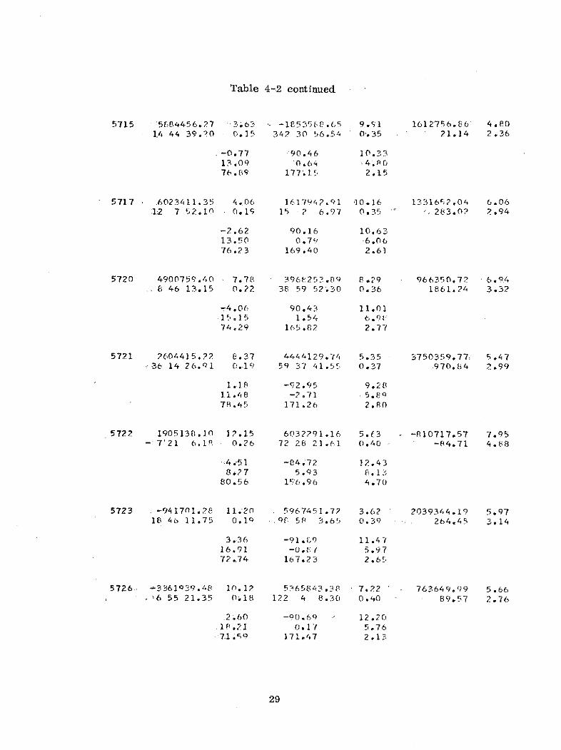
Table 4-2 continued.

5715 5584456.27 -3.6 - -18535&8.65 9.91 1612756.66 4.801A 44 39.?0 0.15 342 30 56.54 0 .35 21.14 2.36

-0.77 -90.46 10.3313.09 '0,64 :4.S076.89 177.15 2.15

5717 6023411.35 4,06 1617942.91 10.16 1331652.04 6.0612 7 52,10 0.1 15 2 6.97 0.35 ' 283.0? 2.94

-2.62 90.16 10.6313.50 0.79 6.0676.23 169.40 2.61

5720 4900759.40 7.78 396f252.9 8.29 966350.72 6.948 46 13.15 0.22 38 59 52.30 0.36 1861.24 3.32

-4.06 90.43 11.0115.15 1.54 6.9t:74.29 165.82 2.77

5721 2604415.22 8.37 4444129.74 5.35 3750359.77 5.4736 14 26. i 0.19 59 37 41.55 0.37 970.84 ?.99

1.18 -92.95 9.2811.48 -2.71 5.8978.45 171.26 2.80

5722 1905138.10 12.15 6032291.16 5.63 -810717.57 7.95- 7'21 6.18 0.26 72 28 21.61 0.40 -84.71 4.68

4.51 -84.72 12.438.7 5.93 F.13

80.56 156.96 4.70

5723 . -941701.28 11.20 -5967451.72 3.62 2039344.19 5.9718 4b 11.75 0.1, .08 58 3,65 0.39 264.45 3.14

3.36 -91 .L9 11.4716.91 -0, 5.9772.,74 167.23 2.65

5726 - 3361039.48 10.12 5365843.38~ 7.22 763649.99 5.66'~6 55 21.35 0618 122 4 8.30 0.40 89.57 2.76

.2.60 -90.69 12.20.18.21 0.17 5.7671.~9 171.47 2,13

29

Table 4-2 continued

5730 -5858556.40 3.75 1394470.97 11.88 2093873.15 6.7419 17 30.43 0.21 166 36 41.12 0.41 17.61 3.63

2.57 -89.73 12.0919.16 1.17 6.74

-70.66 -7.06 3.00

5732 -6099969.36 5.57 -997356.01 13.19 -1568568.44 9.26-14 19 53.78 0.31 189 17 8.88 0.44 37.10 4.93

1.15 -99.62 13.43-1.00 -9.64 9.20

-88.47 -140.45 4.92

5733 -5885321.54 6.71 -244!387.42 12.44 221669.14 10.152 0 18.35 0.33 202 35 17.12 0.43 17.07 5.11

-1.60 -93.89 13.228.05 -4.11 10.18

-81.79 7.29 4.94

5734 -3851774.79 6.08 396407.45 10.09 5051369.83 7.0252 42 49,49 0.21 174 7 26.62 0.54 59.11 6.52

3.43 -86.46 10.1644.38 6.91 7.01

-45.42 0.05 5.98

5735 5,186342.89 7.09 -3654228.01 8.91 -653034.54 6,03- 5 54 58.06 0.20 324 49 55.15 0.35 0.15 3.52

2.02 9?.79 10.85-3.34 2.91 6.0286.10 -28.37 3.49

5736 6118339.51 4.68 -1571766.98 10.47 -878564.03 5.81- 7 58 13.95 0.19 345 35 33,29 0.35 58.44 3,85

0.33 89.37 10.781.22 -0.64 5.85

88.74 -165.40 3.84

5739 4433614.77 4.99 -2268199,51 8.30 3971650.24 4.28-ZA8 3-26..3 023-297 04-.-5 - 8-- - 8-8 .0-8 -2i7

0.50 89.51 9.2010.25 -0.58 4.7179.74 -177.72 2.29

30

Table 4-2 continued

5744 4896433,, 0 3.93 131b615.99 8.81 3856632.15 4.68

37 26 37.53 0,1i 15 2 42.31 0.37 19.20 2.53

-0.72 91].7 9.078.35 1.98 5.17

81.62 176.99 2.44

5907 -449437.73 9.25 -4600 8.92 5.86 4380274.10 6.87

43 '3 56.58 0.28 264 25 14.84 0.41 439.06 2.31

1.57 53, 6. 9.633.06 -36.4" 85.31

-66.56 -9.25 2.26

5911 2307970.19 8.77 -4872779.10 5.44 3394450.16 5.95

32 21 45.28 0.20 295 20 23.3 5 0.37 -36.32 3.19

?.42, 82.68 9.647,93 -7.66 6.20

-81.70 9.53 3.07

5912 11.42624.52 11.07 -610 6 ]0 6 .9]1 4.29 988310.55 8.328 58 26.02 0.28 202 26 54.72 0.36 -14.0 3.88

3.26 94.34 11.15-2.32 4.47 8.4

-85.99 129.84 3.82

5914 2349442.68 21.19 -5576035.64 14.34 2010318.58 18.0818 29 38.59 0.66 292 50 52.62 0.81 -14.77 6.09

0.89 52.65 28.17-12,02 -37.16 13,83-77.94 138.47 5.4?

5915 -744112.30 10.20 -546;236.37 5.45 3192445.85 7. .430 13 45.2Q 0.30 262 14 47.91 0.38 160.55 2.30

-0 75. 8? 41 10. 5-2.33 -7.6? 9.30

-87.55 -169.73 2.26

5923 436335..16 5.84 2t62257.93 7.84 3655387.25 5.2335 11 30.41 0.U1 33 15 50.58 G.36 177.24 2.67

-1.51 90.89 9.2210.49" 1,17 5.6379.4n 172.81 2.49

31

M.T1e1 A c iu.LduI-d ; UUJJLLLLUU

5924 5093544.42 3.35 -565325.16 9.16 3784273.72 4o5136 37 37.26 0.16 353 40 0.28 0.37 13.36 2.60

-0.44 90.36 9.208.44 0.43 4.93

81.55 177.41 2.52

5925 6237359.96 3.26 -1140250.69 10.61 687734.03 5.536 13 53.99 0.18 349 38 24.59 0.35 10.62 2,03

-1.41 90.44 10.739.12 0.66 5.53

80.77 171.72 2.82

5930 -1542545.11 11,P2 6186959.64 4.,0 151849.43 6.181 22 24.24 0.20 103 59 58.83 0,40 20.96 3.29

3.84 -88.31 12.3717.32 2.89 6.3772.23 169.60 2.60

5931 -2423905.19 10.13 5388261.01 5.82 2394895.68 5.7422 11-56.43 0.18 114 13 14.02 0.39 156.14 3.38

2.40 -92.88 11.3320.69 -1.97 5.7369.15 170.80 2.85

5933 -4071567.51 9.82 4714260.45 9.28 -1366510.80 6.04-12 27 14,53 0.?1 130 48 58.33 0.42 77.56 4.07

2.06 -89.61 12.7315.35 0.05 6.5274.51 172.95 3.79

5934 -5367655.52 7.0? 3437875.44 11.01 -225394.72 6.12- 2 2 19.65 0.20 147 21 '0t.52 0.41 78.18 3.18

1.96 -91.43 12.6516.41 -0.85 6.38

-73.47 -8.06 2,69

13 26 22.92 0.18 144 38 5.50 0.t40 96.09 3.04

2.41 -91.38 12.1219,35 -0.53 5.71

-70.40 -8.19 2.46

32

Table 4-2 continued

5937 -4433454.80 F,57 4512935.88 9,14 8099P1.92 5'707 20 41.10 O, 1 134 29 27.56 0.,~0 136.63 2.83

2,32 -91.17 12.2918.44 -0.40 5.79

-71.40 -8.08 2.22

5938 -5915090,05 5.67 2146 66. 0 12.28 -1027 .9 1.2 2 6.83- 9 25 40,37 0.23 160 3 6.35 0.42 74,03 366

2.04 -92.83 12.811.16 -2.43 7.14

-78.65 -13.06 3.64

5941 -546773 0.74 (.62 -238125i.25 11.4P 2254035.33 9.2820 49 55.01 0.30 203 32 1.11 0.43 40.14 5.05

2.37 -84.24 12.4314.3 6.37 9.28

-75.41 -3.39 4.61

6003 -2127794.22 10.51 -3780f,77.57 9,39 4656043.83 8.4547 11 6.64 0,37 240 30 45.02 0.52 341.77 4.11

0.17 -1.02 11.58-1.04 pS.p 10.*188.95 98.34 4.11

6004 -3851773.60 6.14 396407.34 10.14 5051368.22 7.0852'42 49.49 0.21 174 7 26.62 0.54 57.11 6.59

3 ,41. -86.44 10.2044.66 6.C4 7.07

-45.13 0.13 6.05

6007 4433621.08 5.0V -226E'165.4L 8.35 3971658.14 4.4038 45 36.71 0.15 332 54 23.34 0.38 85.30 2.60

0.50 89.59 9.2610. 8 -0.5 . 4.7C479.11 -177.F1 2.49

6008 3623224.46 9.27 -5214237.73 6.40 601514.49 6.985 26 52.72 0.23 204 47 39.59 0.35 -44.07 3.11

1.85 92,.99 10.843.42 2.8f 6.98

-86.11 31.3:9 3. C1

33

6012 -5858551.70 3.88 1394512.64 11.93 2093846.49 6.8119 17 29.56 0.21 166 36 39.69 0.42 13.60 3.77

2.57 -8o,72 12.1419.26 1.18 6.81

-70.55 -7,02 3.16

6015 2604365.53 8.42 4444174,55 5.44 3750336,18 5.5736 14 26.03 0.19 59 37 44.17 0.37 967.81 3.15

1.17 -92,o4 9.3411.73 -2.70 5.9678,21 171.44 2.96

6016 4896384.03 4.02 1316].72.48 8.87 3856674.30 4.7937 26 39.33 0.17 15 2 44.66 0.37 16.25 2.72

-0.71 91.87 9.138.97 1.98 5.25

81.00 177.35 2.62

6042 4900761.23 7.82 3968254.18 8.34 966320.58 7.018 46 12.18 0.22 38 59 52,27 0.30 1858.23 3.45

-4.05 90.45 11.0315,02 1.54 7.0474,42 165.74 2.93

6047 -3361970.26 10.15 5365818.57 7,29 763646.92 5.756 55 21,26 0.18 122 4 9.58 0.40 84.55 2.94

2.62 -90.69 12.2318.27 0.18 5.8471.53 171.44 2.35

6055 6118333.69 4.75 -1571753.54. 10.47 -878606.63 5P89- 7 58 15.37 0.19 345 35 33.67 0.35 55.45 3.95

0.34 89.36 10.780,94 -0.65 5.93

89,00 -160,98 3.94

6059 -588'703 U -A-.---------l3 E. - 12 *S - 2 669.11 10. 202 0 1].35 0.33 202 35 17.12 0,43 16,07 5.21

-1.60 -93,87 13.268.09 -4.09 10.22

-81.75 7.27 5.04

34

Table 4-2 continued

6063 5884455.23 3.77 -1 53504.94 9.95 1612852.31 t.9014 44 42.42 0.16 342 30 59.20 0.35 20.15 2.7

-0.77 90.46 10.3813.26 0.64 4.9076.72 177.21 2.37

6067 5186389.10 7.16 -3653937.17 8.R7 -654292.2,3 6.11- 5 55 39.22 0.20 324 50 3.75 0.35 0.87 3.67

2.03 92.79 10.69-3.22 2.90 6.1086.19 -29.43 3.64

35

5. COMPARISON WITH OTHER SOLUTIONS

Transformation parameters between SECOR-27

and NWL-9D [Anderle, 1973], SAO-III :[Gaposchkin et al., 1973]. and WN-14

solutions[Mueller et al., 1973 ] are included in Tables 5-1, 5-2 and.

5-3 , respectively. The method of computing the parameters is described

in [Kumar, 1972]. In the table the positive angles L4 0, and E are counter-

clockwise rotations about the w, v, and u axes respectively, as viewed from

the end of the positive axis. The scale difference factor is in units of ppM.

Tables 5-1 to 5-3 also contain the variance-covariance matrices,

the correlation coefficients, and the residuals after transformation for the

solutions mentioned above. The unit in the variance-covariance matrix for

the elements corresponding to the rotations in the above tables is radian

squared. The residuals tabulated are those of the Cartesian coordinates

(u, v, w) in meters.

36

Table 5-1 "

Transformation NWL-9D - SECOR-27

SFCOR27 -TO- !-L- .r

DU DV DW DELTA OMECA PSI EPSIL9MEI. RS MET(:RS MFTERS (X1.D+6) SECONrD SFCOUNS SFCD;)S

17.61 0.96 -12.56 0.63 0.42 0.22 0.64

VARIANCE - CORIANCE MATI]X

0 = 1.86

0.9310401 0.212D-01 0.3? D8-01 -0.106D-06 0.3950-07 0.0560-07 -0.1330-07

0.212D-01 0.1400+02 0.2120-01 0.335D-07 0.7.140-07 0. 106O-C07 -0 .252_'-06

0.3280D-01 0.212D-01 0.1050+02 -0.116T-06 -0.424D-08 -0.107:-06 -0.412 -07

-0.1060-06 0.335D0-07 -0.116D-06 0.547D-13 0.5460-17 -0.1240-15 0.536--15

0.395D-07 0.7540-07 -0.4240D-08 0.5460-17 0.523D-13 0.2140-14 -0.460r-15

0.9560-07 0.196D-07 -0.107D-06 -0.1240-15 0.214;0-14 0.5310-13 -0.67h1F--14

-0.1330-07 -0.252D-06 -0.4120-07 0.536D-15 -0.4600-15 -0.5780-14 0.]0'o-l?

CfEFFCIE'TS OF CORRFLA"IIDN

0.1000+01 0.106D-02 0.:31D-02 -0.149D400 0.567D-01 0.1360+00 -0.137 ,:-01

0.1860-02 0. 1000+01 0.1750-02 0.3830-01 0.t10-0 1 0.2280-01 -0.2110+00

0.331D-02 0.1750-02 0.1000+01 -0.1530400 -0.571D-02 -0.14,3')+00 -0.39(0-0

-0.14D90+00 0.3 3 -01 ' -0. 1'0+ 0.100+0! 0.02i- 03 -02 300- - 0) 715n-

0.5670-01 O.31.0-01 -0.57)0-02 0.1020-03 0.1000+01 0.4060-01 -3.b?r,- 02

0.136(+00 0.22D-O01 -0. 43!)+00 --0.2?30-02 0.4,06)-01 0. 1000+01 -o. '1;-1-0 1

-0.1370-01 -0.2110DOO -0.396(-01 0.715[}-02 -0.6PD-(;2 -0.919r-,1 O. (Ol+0o

37

Table 5-1 continued

RFSIDUALS V

V1( SECOR27) V2( NWL-9D ) V - V2

5410 -0.4 0.7 -1.1 700 7.7 -1.2 8.2 -8.0 1.9 -9.35648 6.3 1.4 9.3 708 -11.1 -3.6 -21.0 17.4 5.1 30.35713 1.3 5.6 -0.5 713 -18.1 -19.1 11.5 19.3 24.8 -12.05733 -22.6 27.7 7.1 733 1.7 -0.4 -0.3 -24.3 28.1 7.35736 -0.8 10.5 1.4 716 0.1 -0.2 -0.2 -0.9 10.7 1.55739 1.3 5.6 -0.5 739 -1.2 -19.2 11.2 19.5 24.8 -11.75915 17.7 0.0 13.5 709 -23.1 -0.1 -35.3 40.8 0.2 48.85923 -1.7 -9.8 0.8 719 6.6 13.4 -5.0 -8.3 -23.1 5.95024 0.8 3.4 -0.4 740 -25.6 -9.4 8.0 26.4 12.3 ;-8.45933 2.8 -2.8 2.3 727 -10.4 7.5 -25.7 13.2 -10.3 28.05934 -0.6 2.2 -0.1 729 4.6 -4.3 1.2 -5.2 6.5 -1.35935 1.8 1.2 1.1 728 -13.9 -2.6 -14.2 15.7 3.8 15.36003 -27.3 6.2 -7.7 738 4.0 -1.1 1.8 -31.3 7.3 -9.56004 -2.0 -15.5 -17.? 739 0.9 2.5 5.6 -2.0 -17.0 -22.76007 3.5 9.4 -1.6 727 -16.0 -15.7 9.9 10.5 25.? -11.66008 13.1 2.7 9.5 815 -2.5 -1.1 -3.2 15.6 3.7 12.76012 -1.4 1.9 -2.3 708 10.6 -1.5 5.7 -12.0 3.4 -7.96015 -7.2 -14.8 0.3 817 1.6 8.1 -0.2 -8.8 -22.9 0.56016 6-.8 -4.6 -1.0 812 -6.8 0.9 0.7 13.5 -5.5 -1.76055 -0.8 9.1 0.6 722 0.5 -1.4 -0.3 -1.3 10.5 0.9

38

Table 5-2

Transformation SAO-III - SECOR-27

SECOR27 -TO- SAO-111

DU DV DW DELTA OMEGC PSI FPSILONMETERS METERS METERS (X1.D+6) SECONDS SECONDS SECONDS

17.26 14.44 -13.93 -1.31 0.32 0.58 0.1p

VARIANCE - COVARIANCE MATRIX

at 1.09

0.1770+02 0.1640+00 -0.120D+00 -0.3100-06 0.9890-07 0.2220-06 -0.3670)-07

0.1640+00 0.2270+02 0.725D-01 0.527D-07 0.3140-06 0.4530-07 -0.3960 -06

-0.1200+00 0.7250-01 0.1770+07 -0.1720-06 -0.1190-07 -0.3610-06 -0.1060-06

-0.310D-06 0.5270-07 -0.1720-06 0.976D-13 0.3150-15 0.275D-15 0.3670-15

0.989D-07 0.3140-06 -0.1190-07 0.3150-15 0.1090-12 0.7010-14 -0.1360-13

0.2220-06 0.4530-07 -0.S810-06 0.2750-15 0.7010-14 0.1260-12 -0.1420-13

-0.367D-07 -0.3960-06 -0.1060-06 0.3670-15 -0.1360-13 -0.1420-13 0.1930-12

COEFFICIENTS OF COPR.FLfTION

0.100D+01 0.'17D-02 -0.6810-02 -0.236D+00 0.7120-01 0.1490+00 -0.19ED-01

0.817D-02 0.1000+01 0.362D-02 0.3- 54D-01 0.2000+00 0.26~D-01 -0.1 D+00C

-0.681D-02 0.?62D-0? 0.1000D01 -0.131D+00 -0.8570-02 -0.256+00 -0.571 -01

-0.2360+00 0.3540-01 -0.13D+00 0.1000 01 0.3050-02 0.240D-02 0.2670-02

0.7120-01 0.2000+00 -0.8P57-02 0.3050-02 0.1000+01 0.5990-01 -0.970-01

0.1490+00 0.2680-01 -0.2560400 0.24 80-02 0.5990D-0( 0.100D+01 -0.9] ?0-01

-0.1980-01 -0.189D+00 -0.5710-01 0.2670-02 -0.9370-01 -0.9130-01 0.1'CV+O1

39

RFSIDUALS V

V1( SFCOR27) V2( SAO-III) Vl - V?

6003 -18.2 3.6 5.3 6003 17.5 -4.3 -7.9 -35.7 7.9 13.26004 -0.4 0.3 -0.4 6004 8.2 -2.1 5.1 -8.7 2.5 -5.56007 2.2 3.9 -1.3 6007 -17.8 -11.8 14.3 20.0 15.7 -15.66008 5.3 -0.9 2.9 6008 -18.0 6.8 -17.8 24.3 -7.7 20.76012 0.1 -0.3 -2.6 6012 -1.4 O.q 21.5 1.4 -1.2 -24.?6015 -2.2 -3.0 -0.9 6015 5.9 1.8.9 5.7 -8.2 -21.9 -6.76016 1.3 -3.9 -0.3 6016 -10.9 6.5 1.5 12.2 -10.4 -1.86042 -6.7 -5.9 5.5 6042 11.9 9.3 -12.2 -18.6 -15.2 17.86047 4.8 -0.9 -0.0 6047 -17.2 6.0 0.3 22.0 -6.8 -0.36055 -0.7 2.7 -0.9 6055 5.9 -4.5 4.9 -6.6 7.2 -5.86059 -4.4 9.8 5.3 6059 23.7 -15.7 -12.7 -28.0 25.6 18.06063 -0.6 6.2 -3.0 6063 2.0 -3.0 6.0 -2.6 9.2 -9.06067 10.6 2.2 1.1 6067 -12.1 -1.6 -1.7 22.7 3.8 2.8

40

Table 5-3

Transformation WN14 - SECOR-27

SECOR27 -TO- WN14****** ********t********

DU DV DW DELT. TA OMEGA PSI F PILOPNMETERS METERS METERS (XI.D+6) SFCONDS SECONDS SECrDS

0.76 -5.68 -7.35- 0.64 -0.25 0.29 0.48

VARIANCE - COVARIANCE MATRIX

o= 1.84

0.1550+01 0.6590-02 0.F840-03 -0.5690-08 0.345D-09 0.721D-0 -0.2220-08

0.6590-02 0.249D+01 -0.306D-02 -0.1210-08 0.287)D-o0 0,217D-0F -0.1050-07

0.884D-03 -0.3060D-02 0.1778*+01 -0.8140-08 0.1,50D-09 -0.5390-0 0.279r-0e

-0.569D-08 -0.1210-08 -0.14D-08 .0.3950-14 0.7540-17 -0.4110-17 0.155-17

0.3450-09 0.2870-08 0.185D-09 0.7540-17 0.3770.-14 -0.1220-15 0.113r-i5

0.7210-08 0.217D-08 -0.5390-08 -0.411D-17 -0.122D-15 0.3580-14 -0.1110-14

-0.222D-08 -0.105D-07 0,2790-08 0.1590-17 0.1130-15 -0.1110-14 0.510--14

COEFFICIENTS OF CORRELATION

0.100D+01 0.?360-02 0.5340-03 -0.728,-01 0.4520-02 0.968D-01 -0.2470--01

0.326D-02 0.1000+01 -0.1460-02 -0.1220-01 0.2970-01 0.2300-01 -0.9285-01

0.534D-03 -0.1460-02 0.1000+01 -0.973D-01 0.2270-02 -0.677D-0] 0.2C:1!--0l

-0.720D-01 -0.1220-01 -0.o73D-01 0.1000+01 0.1950-02 -0.1090-02 0.3 51D-ln-

0,452D-02 0.297D-01 0. 227D-02 0 . 1950-02 0. 1000+01 -0.3310-01 0.2561-01

0.o9b0-01 0.2300-01 -0.677D0-01 -0.109D-02 -0.3310-03 0.100+01 --0.?5700P00

-0.2470-01 -0.028.D-01 0, ;2 1 -01 0.351D-03 0.2r,60D-01 -0.257D+00 0 .1o00'4 0i

41

Table 5-3 continued

RFSIDUALS V

VI( SECOR27) V2( WN14 V - V?

5001 15.7 3.6 4.2 5001 -2,4 -1.1 -1.4 18.1 4.8 5.6

5201 -34.0 14.6 -8.1 5201 1,6 -0.8 0.7 -35.6 15.4 -8.P5410 -14.4 8.8 -4.2 5410 4.5 -0.5 1.0 -18.9 9.3 -5.2

5648 12.5 7.6 15.5 5648 -0,8 -0.5 -1.1 13.3 8.1 16.(5712 6.6 6.8 9.9 5712 -0.3 -0.6 -1.8 6.9 7.4 11.75713 10.8 5.4 -7.2 5713 -1.7 -0.4 2.4 12.6 '.7 -Q.65715 5.9 3.9 -1.6 5715 -1.1 -0.2 0.4 7.0 4.1 -7.05717 -1.4 -3.2 5.5 5717 0.3 0.1 -1.1 -1.8 -3.3 6.65720 -7.3 -6.9 11.9 5720 0.5 0.4 -2.0 -7.8 -7.3 13.95721 -1.9 -15.0 -3.2 5721 0.1 2.4 0.& -2.0 -17.4 -4.05722 -4.9 -2.3 16.3 5722 0.4 1.2 -4.8 -5.3 -3.5 21.15773 3.1 -6.5 -0.5 5723 -0.2 2.7 0.2 3.3 -9.1 -0.65726 3.5 -1.8 0.8 5726 -0.2 0.2 -0.2 3.7 -2.0 1.05730 -6.9 4.1 -8.0 .5730 2.1 -0.2. 1.7 -9.0 4.3 -9.8

5732 0.4 18.1 9.4 5732 -0.2 -1.3 -1.9 0.5 19.5 11.35733 -9.2 21.3 8.9 5733 1.6 -1.2 -1.3 -10.8 22.5 10.25734 -12.1 0.9 -14.5 5734 2.4 -0.1 4.5 -14.5 1.0 -16.95735 -2.2 7.1 7.6 5735 0.2 -0.4 -1.3 -2.4 7.5 0.05736 -6.1 5.5 6.2 5736 1.5 -0.3 -1.4 -7.5 5.8 7.65739 10.8 5.3 -7.2 5739 -1.7 -0.4 2.4 12.5 5.7 -9.65744 5.2 -11.2 -3.6 5744 -1.1 0.7 0 .9 6.3 -11.9 -4.55907 16.1 2.8 5.4 5907 -3.3 -0.8 -2.4 19.4 3.6 7.85911 15.1 3.9 3.1 5911 -1.3 -0.7 -0.8 16.4 4.7 3.95912 10.7 2.9 13.7 5912 -O. -1.9 -3.3 11.6 4.8 17.05914 5.5 8.9 12.7 5914 -1.4 -2.1 -1.5 6.9 11.0 14.15915 15.8 1.1 10.9 5915 -2.2 -0.5 -3.9 18.0 1.7 14.75923 1.5 -13.1 -0.6 5923 -0.2 0.9 0.1 1.7 -14.0 -0.75924 8.6 -6.1 -6.0 5924 -2.7 0.5 2.5 11.3 -6.6 -8.55925 0.3 5.4 2.? 5025 -0.1 -0.3 -0.7 0.4 5.7 2.95930 5.4 -0.3 5.9 5930 -0.3 0.1 -1.8 5.7 -0.4 7.85931 2.4 -9.6 -4.1 5931 -0.1 1.8 1.6 2.5 -11.4 -5.75933 6.6 3.3 4.9 5933 -0.7 -0.4 -1.9 7.3 3.7 6.85934 1.0 5.2 0.6 5934 -0.1 -0.3 -0.2 1.2 5.5 0.75935 -1.2 1.5 -3.3 5935 0.1 -0.1 0.8 -1.3 1.6 -4.15937 1.8 0.8 -0.5 5937 -0.1 -0.0 0.2 1.Q 0.9 -0.75938 0.0 8.2 1.7 5038 -0.0 -0.5 -0.4 0.1 8.7 ?.15941 -19.9 17.7 4.4 5941 2.9 -1.0 -0.7 -22.7 18.7 5.1

42

Table 5-3 continued

RESIDU.LS V

V1( SFCOP27) V2( WN14 ) Vi - V2- - - - -- - - - - - - - - -

6003 -34.5 15.0 -8.5 6003 1.4 -0.7 0.6 -3 .9 15.7 -(.16004 -11.P 1.1 -14.5 6004 2.3 -0.1 4.4 -14.2 1.2 -1f,96007 12.2 6.1 -7.2 6007 -2.0 -0.4 2.3 14.1 6.5 -0.56008 6.7 7.0 10.3 6008 -0.4 -0.7 -1.8 7.0 7.7 12.16012 -6.5 3.9 -8.4 6012 2.0 -0.2 1.8 -8.4 4.1 -10.26015 -3.6 -16.0 -3.4 6015 0.2 2.6 0. i -3.8 -18.6 -4.?6016 5.6 -10.6 -3.8 6016. -1.1 0.6 0.8 6.7 -11.3 -4.76042 -7.5 -7.4 12.5 60,,42 0.5 0.5 -2.1 -V.0 -7.9 14.L6047 4.1 -2.1 0.8 6047 -0.2 0.2 -0.2 4.4 -2.3 1.06055 -6.3 5.6 5.9 6055 1.5 -0.3 -1.4 -7.8 5.9 7.36059 -q.7 22.3 9.3 6059 1.6 -1.2 -1.3 -11.3 23.5 10.66063 5.5 4.5 -2.0 6063 -1.2 -0.2 0.5 6.7 4.7 -2.',6067 -2.0 6.7 7.3 6067 0.2 -0.4 -1.3 -2.1 7.1 18.7

43

6. CONCLUSIONS

The average standard deviations of the coordinates and the heights

for SECOR-27 solution (excluding stations 5648 and 5914) are:

Position = .5m

0 = 3.4maHeight

The above values when compared with the corresponding values of

WN14 solution [(Table 5.3-2) Mueller et al., 1973] show that a further signi-

ficant improvement in the SECOR network determination is possible, if it

is done as part of the world net.

The standard deviations of stations 5648 and 5914 (Table 4.2) indi-

cate that these two stations are poorly determined compared to the other

stations in the network -- a pattern which is also present in the WN14

solution [(Table 5.2-2) Mueller et al., 1973].

The semi-diameter of the level ellipsoid best fitting the geoid (de-

fined through the SECOR 27 undulations) is 6378140.4±7.7 m (1/f = 298.2495).

44

REFERENCES

Anderle, R. J. (1973). "Transformation of Terrestrial Survey Data toDoppler Satellite Datum." Journal of Geophysical Research, preprint.

Blaha, Georges. (1971). "Inner Adjustment Constraints with Emphasis onRange Observations." Reports of the Department of Geodetic Science,No. 148. The Ohio State University, Columbus.

Blaha, Georges. (1971a). "Investigations of Critical Configurations forFundamental Range Networks." Reports of the Department of GeodeticScience, No. 150. The Ohio State University, Columbus.

CSC. (1971). NASA Directory of Observation Station Locations, Vol. 1 and2, second edition. Prepared by Computer Sciences Corporation, FallsChurch, Virginia, for Metric Data Branch, Network Computing andAnalysis Division, Goddard Space Flight Center, Greenbelt, Maryland.

CSC. (1972/73). Correction Sheets to NASA Directory of ObservationStation Locations, Vol. 1 and 2. Prepared by Computer SciencesCorporation, Falls Church, Virginia.

Gaposchkin, E.M., G. Veis and J. Latimer. (1973). "Smithsonian Institu-tion Standard Earth III Coordinates.? Presented at First InternationalSymposium, The Use of Artificial Satellites for Geodesy and Geodynamics,Athens, Greece, May 14-21.

Krakiwsky, Edward J. and Allen J. Pope. (1967). "Least Squares Adjustmentof Satellite Observations for Simultaneous Directions or Ranges, Part 1of 3: Formulation of Equations." Reports of the Department of GeodeticScience, No. 86, The Ohio State University, Columbus.

Kumar, Muneendra. (1972). "Coordinate Transformation by MinimizingCorrelations Between Parameters." Reports of the Department of GeodeticScience, No. 184, The Ohio State University, Columbus.

Mueller, Ivan I. (1968). "Global Satellite Triangulation and Trilateration,"Bulletin Geodesique, 87.

Mueller, Ivan I., M. Kumar, J. P. Reilly, N. Saxena, T. Soler. (1973)."Global Satellite Triangulation and Trilateration for the National GeodeticSatellite Program." Reports of the Department of Geodetic Science, No.199, The Ohio State University, Columbus.

45

Rapp, R. H. (1973). "Comparison of Least Squares and Collocation EstimatedPotential Coefficients." Reports of the Department of Geodetic Science,No. 200, The Ohio State University, Columbus.

Reilly, J.P., C.R. Schwarz, M.C. Whiting. (1972). "The Ohio State

University Geometric and Orbital (Adjustment) Program (OSUGOP) forSatellite Observations." Reports of the Department of Geodetic Science,No. 190, The Ohio State University, Columbus.

Rinner, K. et al. (1967). "Beitrige zur Theorie der Geoditischen Netze imRaum." Deutsche Geodatische Kommission, Reihe A, Heft 61, Munich.

Rutscheid, Erick H. (1972). "Preliminary Results of the Secor Equatorial

Network, " The Use of Artificial Satellites for Geodesy, edited by S.W.Henriksen et al., Geophysical Monograph 15, American GeophysicalUnion, Washington, D.C.

Tsimis, Emmanuel. (1973). "Critical Configurations (Determinantal Loci)for Range and Range-Difference Satellite Networks." Reports of theDepartment of Geodetic Science, No. 191, The Ohio State University,Columbus.

46