Concurrency theorytypes to reason about processes: subtyping, receptiveness

from process calculi to programming languagessome slides to navigate through the literature

Francesco Zappa Nardelli

INRIA Paris-Rocquencourt, MOSCOVA research team

francesco.zappa nardelli@inria.fr

together with

Frank Valencia (INRIA Futurs) Roberto Amadio (PPS) Emmanuel Haucourt (CEA)

MPRI - Concurrency November 6, 2008

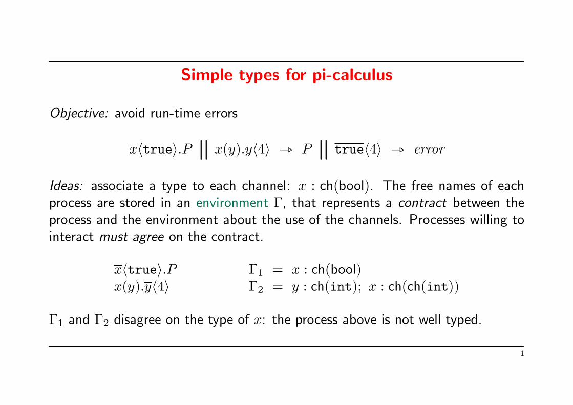
Simple types for pi-calculus

Objective: avoid run-time errors

x〈true〉.Pn

x(y).y〈4〉 _ Pn

true〈4〉 _ error

Ideas: associate a type to each channel: x : ch(bool). The free names of eachprocess are stored in an environment Γ, that represents a contract between theprocess and the environment about the use of the channels. Processes willing tointeract must agree on the contract.

x〈true〉.P Γ1 = x : ch(bool)x(y).y〈4〉 Γ2 = y : ch(int); x : ch(ch(int))

Γ1 and Γ2 disagree on the type of x: the process above is not well typed.

1

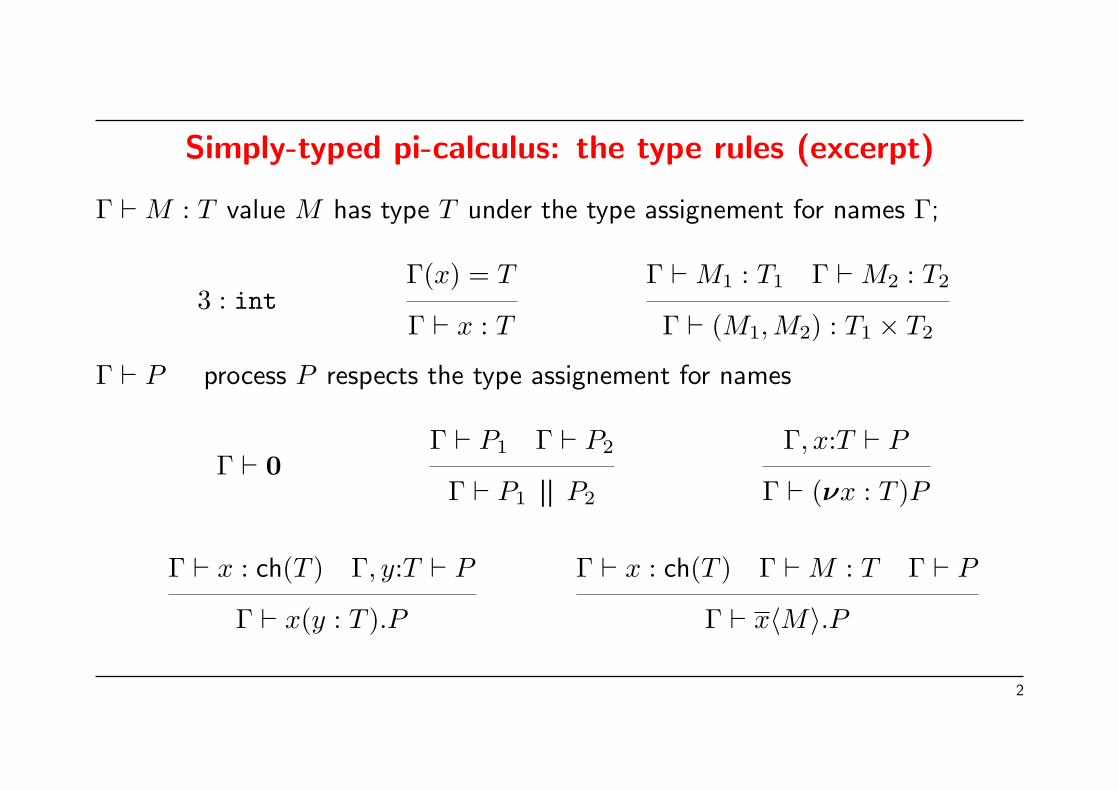
Simply-typed pi-calculus: the type rules (excerpt)

Γ ` M : T value M has type T under the type assignement for names Γ;

3 : intΓ(x) = T

Γ ` x : T

Γ ` M1 : T1 Γ ` M2 : T2

Γ ` (M1,M2) : T1 × T2

Γ ` P process P respects the type assignement for names

Γ ` 0Γ ` P1 Γ ` P2

Γ ` P1

fP2

Γ, x:T ` P

Γ ` (νx : T )P

Γ ` x : ch(T ) Γ, y:T ` P

Γ ` x(y : T ).P

Γ ` x : ch(T ) Γ ` M : T Γ ` P

Γ ` x〈M〉.P

2

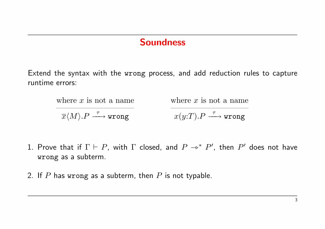
Soundness

Extend the syntax with the wrong process, and add reduction rules to captureruntime errors:

where x is not a name

x〈M〉.P τ−−→ wrong

where x is not a name

x(y:T ).P τ−−→ wrong

1. Prove that if Γ ` P , with Γ closed, and P _∗ P ′, then P ′ does not havewrong as a subterm.

2. If P has wrong as a subterm, then P is not typable.

3

Types to reason about processes

Specification and an implementation of the factorial function:

Spec = !f(x, r).r〈fact(x)〉Imp = !f(x, r).if x = 0 then r〈1〉 else (νr′)f〈x− 1, r′〉.r′(m).r〈x ∗m〉

In general, Spec 6∼= Imp. (Why?)

Idea: the channel f should be write-only for the environment.

4

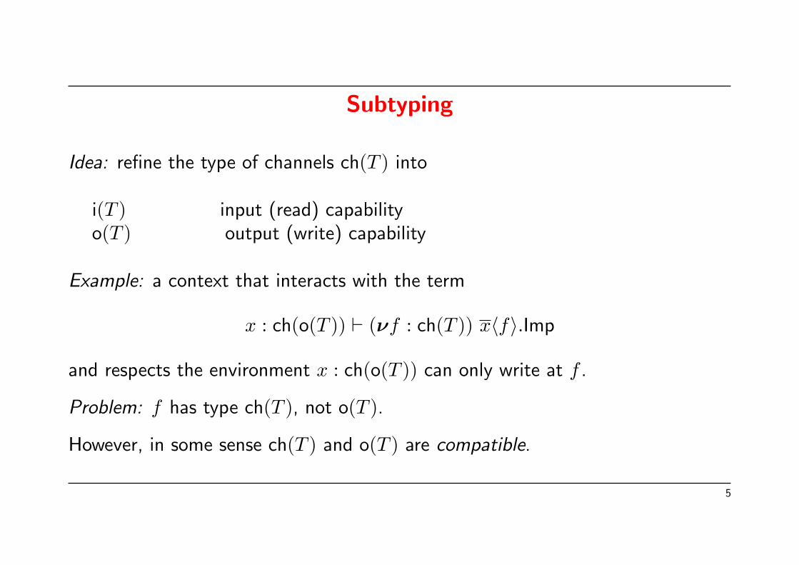
Subtyping

Idea: refine the type of channels ch(T ) into

i(T ) input (read) capabilityo(T ) output (write) capability

Example: a context that interacts with the term

x : ch(o(T )) ` (νf : ch(T )) x〈f〉.Imp

and respects the environment x : ch(o(T )) can only write at f .

Problem: f has type ch(T ), not o(T ).

However, in some sense ch(T ) and o(T ) are compatible.

5

Subtyping

We say that a type T1 is a subtype of a type T2, denoted T1 <: T2 if it is safe touse a value of type T1 in all contexts that expect a value of type T2. For instance:

• int <: float: the value 3 can safely be used in the context sqr(−).

• float 6<: int: the value 3.14 cannot be used in the context − mod 3 becausemod is not defined over floats.

• a:int; b:int <: a : int: a context accepting records containing the labela will just ignore the existence of the label b.

• ch(T ) <: o(T ): a context expecting a channel of type o(T ) will just ignore theread capability available.

6

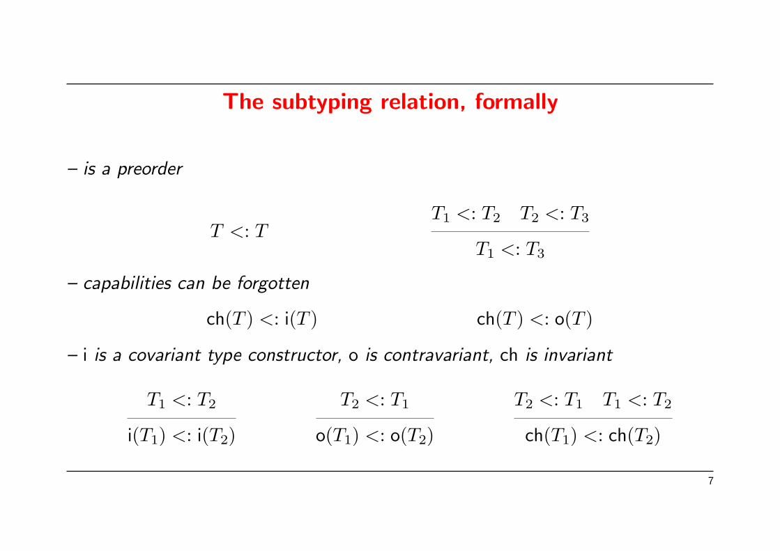
The subtyping relation, formally

– is a preorder

T <: TT1 <: T2 T2 <: T3

T1 <: T3

– capabilities can be forgotten

ch(T ) <: i(T ) ch(T ) <: o(T )

– i is a covariant type constructor, o is contravariant, ch is invariant

T1 <: T2

i(T1) <: i(T2)

T2 <: T1

o(T1) <: o(T2)

T2 <: T1 T1 <: T2

ch(T1) <: ch(T2)

7

Subtyping, ctd.

Intuition: if x : o(T ) then it is safe to send along x values of of a subtype of T .Dually, if x : i(T ) then it is safe to assume to assume that values received alongx belong to a supertype of T .

Type rules must be updated as follows:

Γ ` x : i(T ) Γ, y:T ` P

Γ ` x(y : T ).P

Γ ` x : o(T ) Γ ` M : T Γ ` P

Γ ` x〈M〉.P

Γ ` M : T1 T1 <: T2

Γ ` M : T2

8

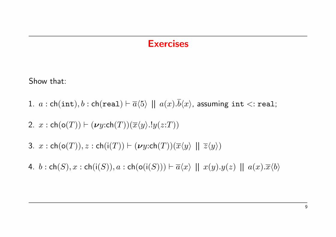
Exercises

Show that:

1. a : ch(int), b : ch(real) ` a〈5〉f

a(x).b〈x〉, assuming int <: real;

2. x : ch(o(T )) ` (νy:ch(T ))(x〈y〉.!y(z:T ))

3. x : ch(o(T )), z : ch(i(T )) ` (νy:ch(T ))(x〈y〉f

z〈y〉)

4. b : ch(S), x : ch(i(S)), a : ch(o(i(S))) ` a〈x〉f

x(y).y(z)f

a(x).x〈b〉

9

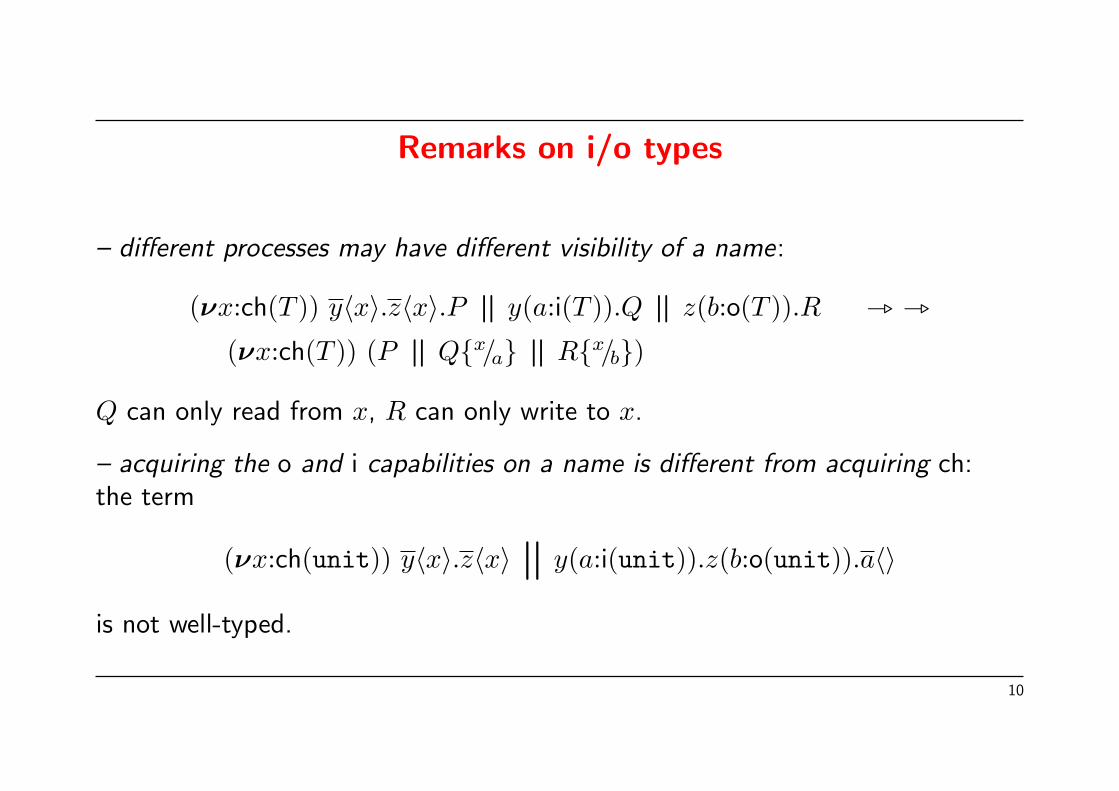
Remarks on i/o types

– different processes may have different visibility of a name:

(νx:ch(T )) y〈x〉.z〈x〉.Pf

y(a:i(T )).Qf

z(b:o(T )).R _ _

(νx:ch(T )) (Pf

Qx/af

Rx/b)

Q can only read from x, R can only write to x.

– acquiring the o and i capabilities on a name is different from acquiring ch:the term

(νx:ch(unit)) y〈x〉.z〈x〉n

y(a:i(unit)).z(b:o(unit)).a〈〉

is not well-typed.

10

Types for reasoning

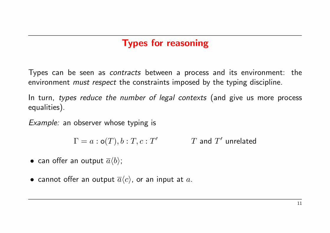
Types can be seen as contracts between a process and its environment: theenvironment must respect the constraints imposed by the typing discipline.

In turn, types reduce the number of legal contexts (and give us more processequalities).

Example: an observer whose typing is

Γ = a : o(T ), b : T, c : T ′ T and T ′ unrelated

• can offer an output a〈b〉;

• cannot offer an output a〈c〉, or an input at a.

11

A typed contextual equivalence, informally

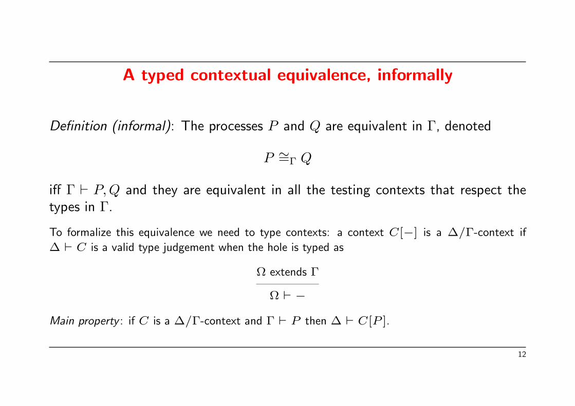
Definition (informal): The processes P and Q are equivalent in Γ, denoted

P ∼=Γ Q

iff Γ ` P,Q and they are equivalent in all the testing contexts that respect thetypes in Γ.

To formalize this equivalence we need to type contexts: a context C[−] is a ∆/Γ-context if

∆ ` C is a valid type judgement when the hole is typed as

Ω extends Γ

Ω ` −

Main property : if C is a ∆/Γ-context and Γ ` P then ∆ ` C[P ].

12

Semantic consequences of i/o types

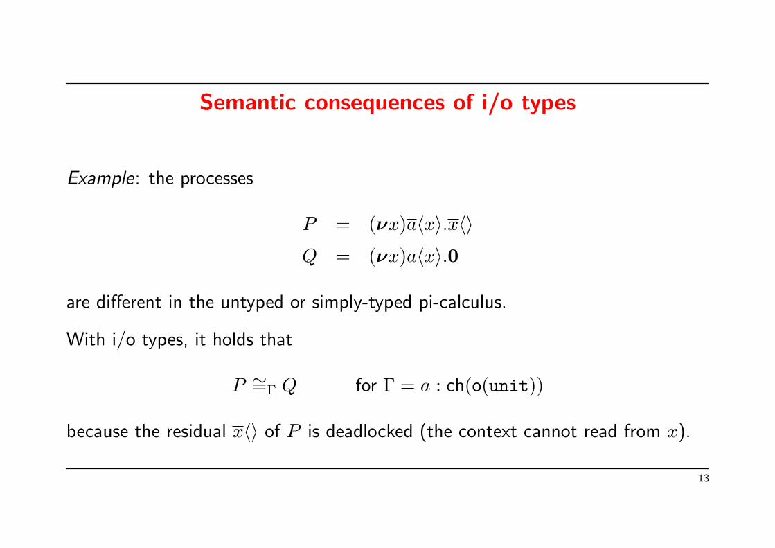
Example: the processes

P = (νx)a〈x〉.x〈〉Q = (νx)a〈x〉.0

are different in the untyped or simply-typed pi-calculus.

With i/o types, it holds that

P ∼=Γ Q for Γ = a : ch(o(unit))

because the residual x〈〉 of P is deadlocked (the context cannot read from x).

13

Semantic consequences of i/o types, ctd.

Back to the factorial function:

Spec = !f(x, r).r〈fact(x)〉Imp = !f(x, r).if x = 0 then r〈1〉 else (νr′)f〈x− 1, r′〉.r′(m).r〈x ∗m〉

With i/o types, we can protect the input end of the function, obtaining

(νf)a〈f〉.Spec ∼=Γ (νf)a〈f〉.Imp

for Γ = a : ch(o(int× o(int))).

Which is the type that I omitted after the restriction of r′? .

14

Semantic consequences of i/o types, ctd.

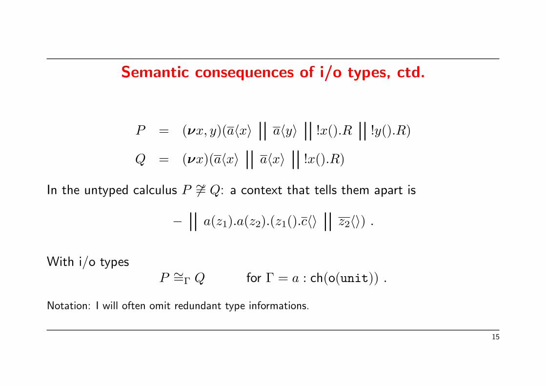
P = (νx, y)(a〈x〉n

a〈y〉n

!x().Rn

!y().R)

Q = (νx)(a〈x〉n

a〈x〉n

!x().R)

In the untyped calculus P 6∼= Q: a context that tells them apart is

−n

a(z1).a(z2).(z1().c〈〉n

z2〈〉) .

With i/o typesP ∼=Γ Q for Γ = a : ch(o(unit)) .

Notation: I will often omit redundant type informations.

15

Challenge: a labelled equivalence

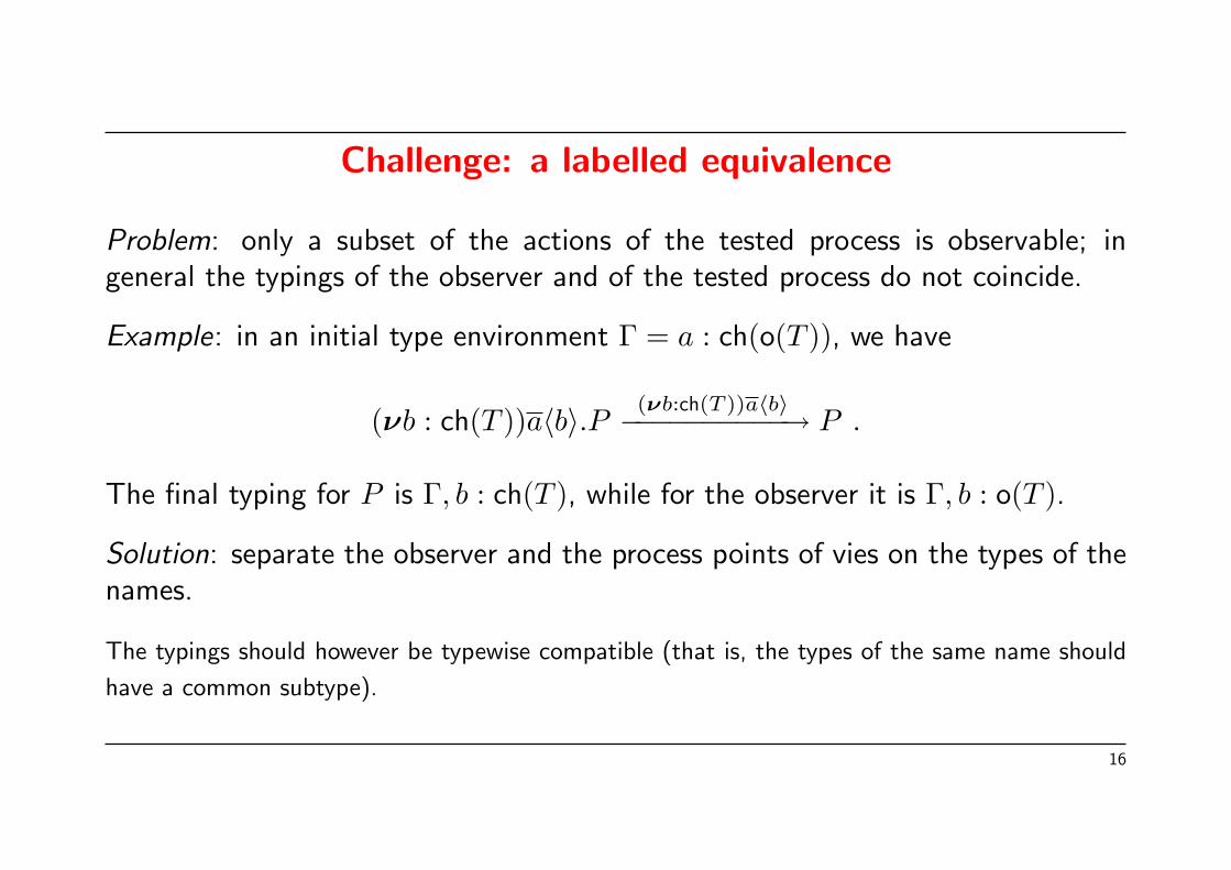
Problem: only a subset of the actions of the tested process is observable; ingeneral the typings of the observer and of the tested process do not coincide.

Example: in an initial type environment Γ = a : ch(o(T )), we have

(νb : ch(T ))a〈b〉.P (νb:ch(T ))a〈b〉−−−−−−−−−−→ P .

The final typing for P is Γ, b : ch(T ), while for the observer it is Γ, b : o(T ).

Solution: separate the observer and the process points of vies on the types of thenames.

The typings should however be typewise compatible (that is, the types of the same name should

have a common subtype).

16

Challenge: a labelled equivalence, ctd.

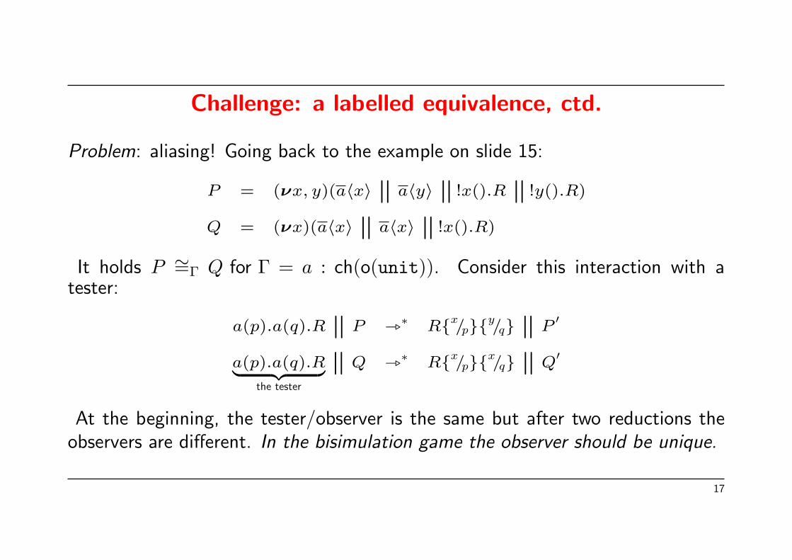
Problem: aliasing! Going back to the example on slide 15:

P = (νx, y)(a〈x〉n

a〈y〉n

!x().Rn

!y().R)

Q = (νx)(a〈x〉n

a〈x〉n

!x().R)

It holds P ∼=Γ Q for Γ = a : ch(o(unit)). Consider this interaction with atester:

a(p).a(q).Rn

P _∗ Rx/py

/qn

P′

a(p).a(q).R| z the tester

nQ _∗ Rx

/px/q

nQ′

At the beginning, the tester/observer is the same but after two reductions theobservers are different. In the bisimulation game the observer should be unique.

17

Aliasing, ctd.

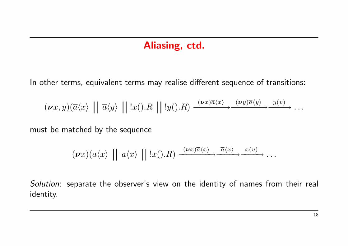
In other terms, equivalent terms may realise different sequence of transitions:

(νx, y)(a〈x〉n

a〈y〉n

!x().Rn

!y().R)(νx)a〈x〉−−−−−−−→ (νy)a〈y〉−−−−−−−→ y(v)−−−−→ . . .

must be matched by the sequence

(νx)(a〈x〉n

a〈x〉n

!x().R)(νx)a〈x〉−−−−−−−→ a〈x〉−−−−→ x(v)−−−−→ . . .

Solution: separate the observer’s view on the identity of names from their realidentity.

18

Digression

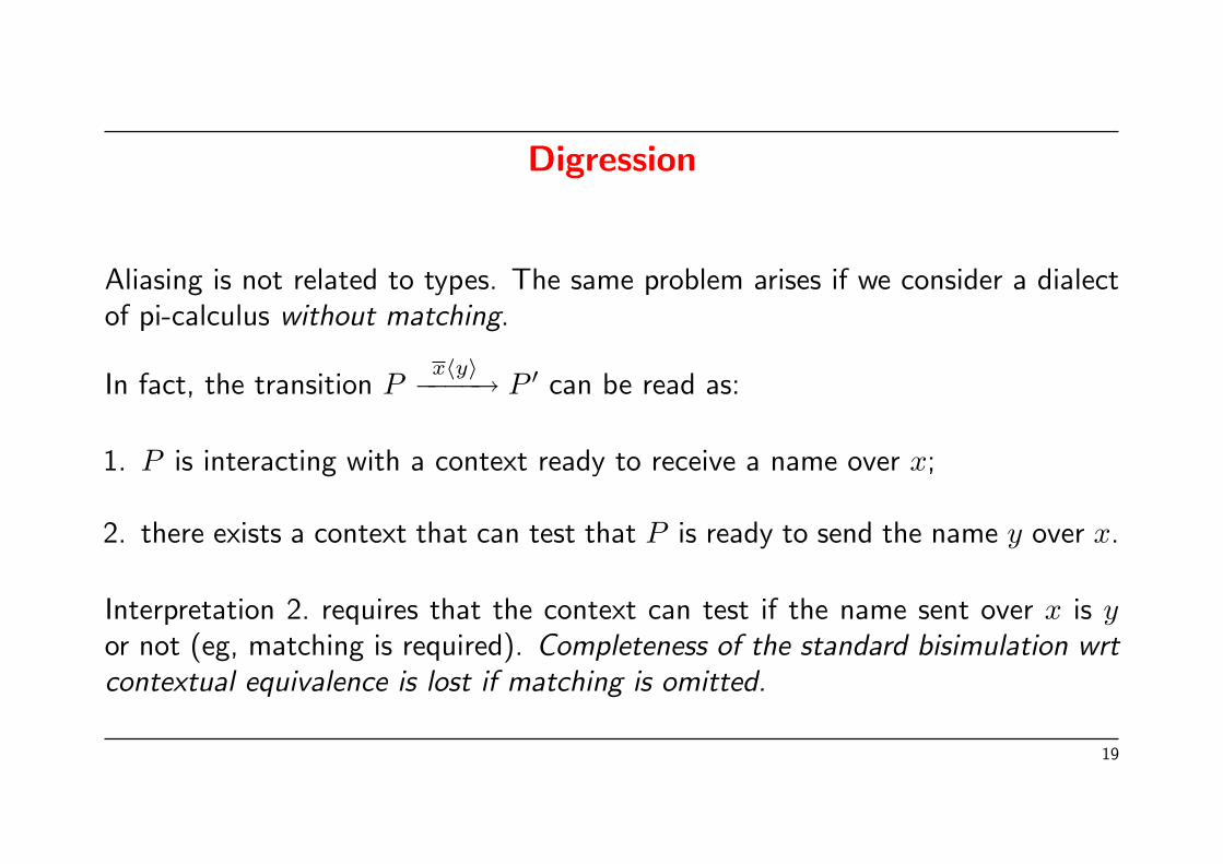
Aliasing is not related to types. The same problem arises if we consider a dialectof pi-calculus without matching.

In fact, the transition Px〈y〉−−−−→ P ′ can be read as:

1. P is interacting with a context ready to receive a name over x;

2. there exists a context that can test that P is ready to send the name y over x.

Interpretation 2. requires that the context can test if the name sent over x is yor not (eg, matching is required). Completeness of the standard bisimulation wrtcontextual equivalence is lost if matching is omitted.

19

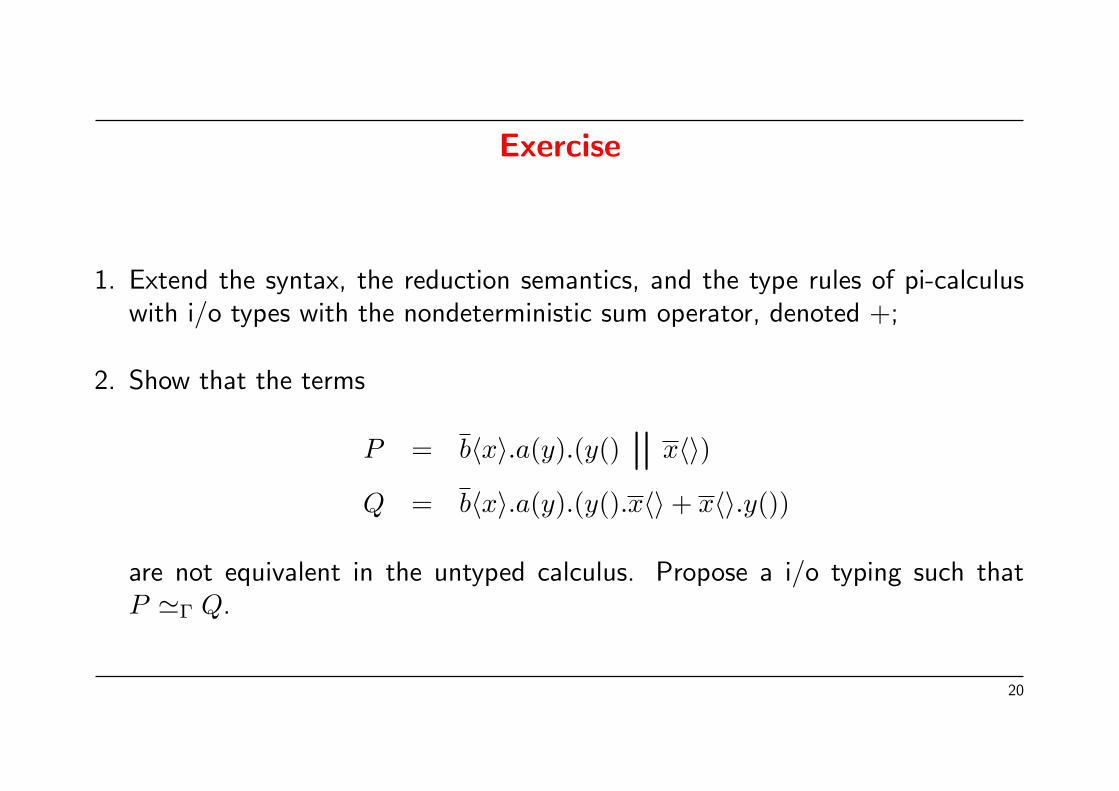
Exercise

1. Extend the syntax, the reduction semantics, and the type rules of pi-calculuswith i/o types with the nondeterministic sum operator, denoted +;

2. Show that the terms

P = b〈x〉.a(y).(y()n

x〈〉)

Q = b〈x〉.a(y).(y().x〈〉+ x〈〉.y())

are not equivalent in the untyped calculus. Propose a i/o typing such thatP 'Γ Q.

20

Receptiveness

A local environment:(νx)(!x(y).R

nQ)

(Q and R have only the output capability on x).

The name x is stateless, and its input end is always available: x is uniformlyreceptive.

Uniform receptiveness occurs when modelling functions, objects, RPC protocols,etc. It is a common idiom in programming languages based on pi-calculus (Pict,Join, Blue): def x(y) = R in Q. Variant: linear receptiveness: x is used atmost once.

It is possible to impose receptiveness using syntactical constraints, or a typesystem.

21

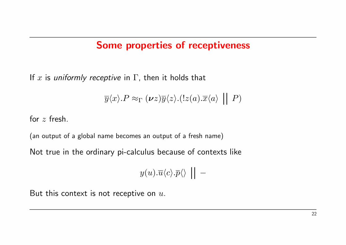
Some properties of receptiveness

If x is uniformly receptive in Γ, then it holds that

y〈x〉.P ≈Γ (νz)y〈z〉.(!z(a).x〈a〉n

P )

for z fresh.

(an output of a global name becomes an output of a fresh name)

Not true in the ordinary pi-calculus because of contexts like

y(u).u〈c〉.p〈〉n−

But this context is not receptive on u.

22

Some properties of receptiveness, ctd.

If x is uniformly receptive in Γ, then it holds that

x〈v〉.P ≈Γ x〈v〉n

P

(makes a synchronous communication into an asynchronous one).

If P _ P ′ by means of a communication at x, then

P ≈Γ P ′

(insensitiveness to internal reductions)

Remark: all names uniformly receptive ⇒ confluence.

23

Factorial function again

S1 = !f(x:int, y:int, r:lrec(int)). if x = 0 then r〈y〉else (νr′)(f〈x− 1, x ∗ y, r′〉.r′(m).r〈m〉)

S2 = !f(x:int, y:int, r:lrec(int)). if x = 0 then r〈y〉else f〈x− 1, x ∗ y, r〉

Exercise: Give a (non-well typed) context that shows that S1 and S2 are notequivalent.

However, taking into account the receptiveness of f, r and r′, S1 and S2 arebehaviourally equivalent (tail-call optimisation).

24

References

Milner: The polyadic pi-calculus - a tutorial, ECS-LFCS-91-180.

Pierce, Sangiorgi: Typing and subtyping for mobile processes, LICS ’93.

Boreale, Sangiorgi: Bisimulation in name-passing calculi without matching, LICS’98.

Sangiorgi, Walker: The pi-calculus, CUP.

...there is a large literature on the subject. The articles above have been reported because they

are explicitely mentioned in this lecture.

25

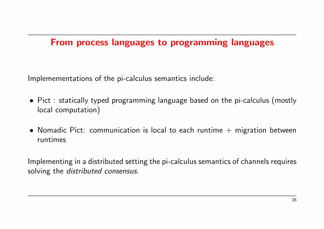
From process languages to programming languages

Implemementations of the pi-calculus semantics include:

• Pict : statically typed programming language based on the pi-calculus (mostlylocal computation)

• Nomadic Pict: communication is local to each runtime + migration betweenruntimes

Implementing in a distributed setting the pi-calculus semantics of channels requiressolving the distributed consensus.

26

Erlang

An dinamically typed language a la Lisp;

each thread has a unique identifier;

each thread has one channel, identified by the thread id;

send: id!msg

receive:

receivepatt1 -> action1patt2 -> action2...

end.

27

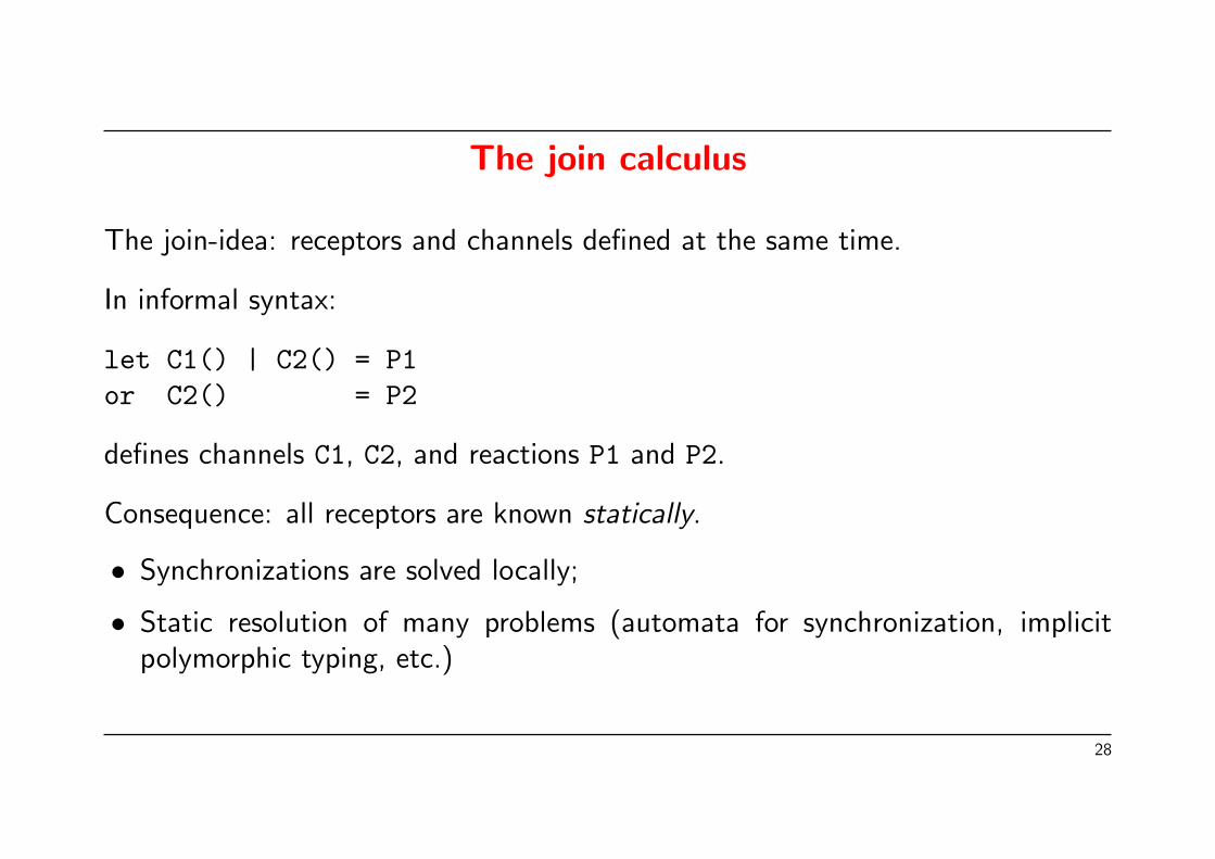
The join calculus

The join-idea: receptors and channels defined at the same time.

In informal syntax:

let C1() | C2() = P1or C2() = P2

defines channels C1, C2, and reactions P1 and P2.

Consequence: all receptors are known statically.

• Synchronizations are solved locally;

• Static resolution of many problems (automata for synchronization, implicitpolymorphic typing, etc.)

28

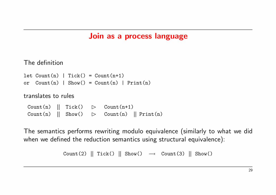
Join as a process language

The definition

let Count(n) | Tick() = Count(n+1)or Count(n) | Show() = Count(n) | Print(n)

translates to rules

Count(n)f

Tick() Count(n+1)Count(n)

fShow() Count(n)

fPrint(n)

The semantics performs rewriting modulo equivalence (similarly to what we didwhen we defined the reduction semantics using structural equivalence):

Count(2)f

Tick()f

Show() −→ Count(3)f

Show()

29

(the new) JoCaml

• An extension of OCaml 3.10;

• distributed asynchronous channels (synchronous channels by CPS);

• polymorphic typing a la ML;

• easy encoding of concurrent programming constructs.For instance, what does the code below do?

type ’a buffer = get : unit -> ’a ; put : ’a -> unit ;

let create_buff () =def some(v) & get() = none() & reply v to getor none() & put(v) = some(v) & reply () to put inspawn none() ; get = get ; put = put ;

30

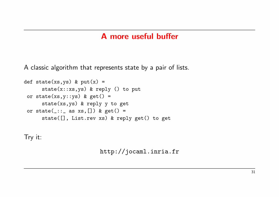
A more useful buffer

A classic algorithm that represents state by a pair of lists.

def state(xs,ys) & put(x) =state(x::xs,ys) & reply () to put

or state(xs,y::ys) & get() =state(xs,ys) & reply y to get

or state(_::_ as xs,[]) & get() =state([], List.rev xs) & reply get() to get

Try it:

http://jocaml.inria.fr

31

Navigating through the literature

Pi-calculus literature describes zillions of slightly different languages, semantics,equivalencies.

Some slides for not getting lost.

32

Barbed congruence vs. reduction-closed barbed congruence

Let barbed equivalence, denoted ∼=•, be the largest symmetric relation that isbarb preserving and reduction closed. Barbed equivalence is not preserved bycontext, so define barbed congruence, denoted ∼=c, as

(P,Q) : C[P ] ∼=• C[Q] for every context C[-].

• Barbed congruence is more natural and less discriminating than reduction-closed barbed congruence (for pi-calculus processes).

• Completeness of bisimulation for image-finite processes holds with respect tobarbed congruence, but its proof requires transfinite induction.

33

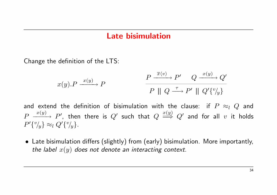
Late bisimulation

Change the definition of the LTS:

x(y).Px(y)−−−−→ P

Px〈v〉−−−−→ P ′ Q

x(y)−−−−→ Q′

Pf

Qτ−−→ P ′ f

Q′v/y

and extend the definition of bisimulation with the clause: if P ≈l Q and

Px(y)−−−−→ P ′, then there is Q′ such that Q

x(y)=⇒ Q′ and for all v it holds

P ′v/y ≈l Q′v/y.

• Late bisimulation differs (slightly) from (early) bisimulation. More importantly,the label x(y) does not denote an interacting context.

34

Ground bisimulation

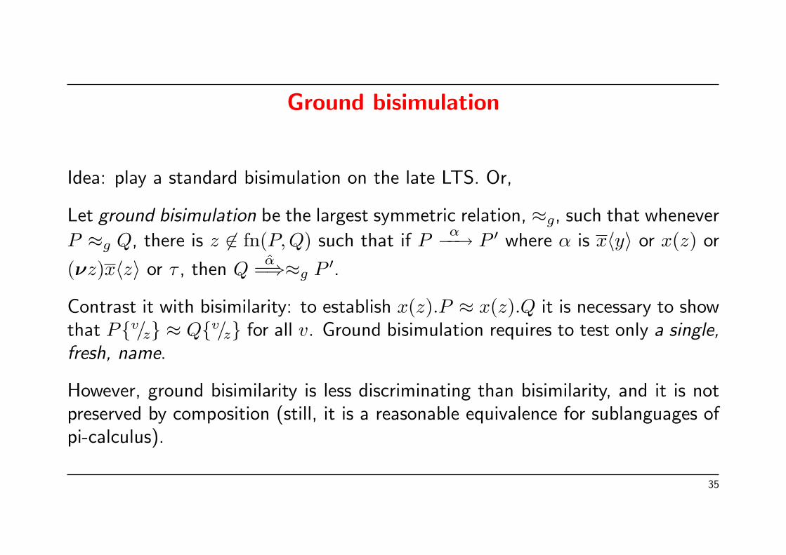
Idea: play a standard bisimulation on the late LTS. Or,

Let ground bisimulation be the largest symmetric relation, ≈g, such that whenever

P ≈g Q, there is z 6∈ fn(P,Q) such that if Pα−−→ P ′ where α is x〈y〉 or x(z) or

(νz)x〈z〉 or τ , then Qα=⇒≈g P ′.

Contrast it with bisimilarity: to establish x(z).P ≈ x(z).Q it is necessary to showthat Pv/z ≈ Qv/z for all v. Ground bisimulation requires to test only a single,fresh, name.

However, ground bisimilarity is less discriminating than bisimilarity, and it is notpreserved by composition (still, it is a reasonable equivalence for sublanguages ofpi-calculus).

35

Open bisimulation

Full bisimilarity is the closure of bisimilairty under substitutions, and is acongruence with respect to all contexts. Unfortunately, full bisimilarity is notdefined co-inductively.

Question: can we give a co-inductive definition of a useful congruence?

Yes, with open bisimulation.

Idea: (on the restriction free calculus) let ./ be the largest symmetric relation such

that whenever P ./ Q and σ is a substitution, Pσα−−→ P ′ implies Qσ

α=⇒./ P ′.

It is possible to avoid the σ quantification by means of an appropriate LTS.

36

Subcalculi

Idea: In pi-calculus contexts have a great discriminating power. It may be usefulto consider other languages in which contexts ”observe less”, so that we havemore equations.

Asynchronous pi-calculus: no continuation after an output prefix.

Localized pi-calculus: given x(y).P , the name y is not used as subject of aninput prefix in P .

Private pi-calculus: only output of new names.

37

Distribution, action at distance, and mobility

The parallel composition operator of CCS and pi-calculus does not specify whetherthe concurrent threads are running on the same machine, or on different machinesconnected by a network.

Some phenomena typical of distributed systems require a finer model, thatexplicitly keeps track of the spatial distribution of the processes.

We will briefly sketch two models that have been proposed: DPI (Hennessy andRiely, 1998) and Mobile Ambients (Cardelli and Gordon, 1998).

The aim of this section is to get a glimpse of more complex process languages, and to rediscover

the idea of “transitions in an LTS characterise the interactions a term can have with a context”

in this setting.

38

DPI, design choices

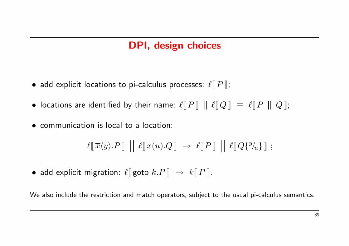
• add explicit locations to pi-calculus processes: `[[ P ]];

• locations are identified by their name: `[[ P ]]f

`[[ Q ]] ≡ `[[ Pf

Q ]];

• communication is local to a location:

`[[ x〈y〉.P ]]n

`[[ x(u).Q ]] _ `[[ P ]]n

`[[ Qy/u ]] ;

• add explicit migration: `[[ goto k.P ]] _ k[[ P ]].

We also include the restriction and match operators, subject to the usual pi-calculus semantics.

39

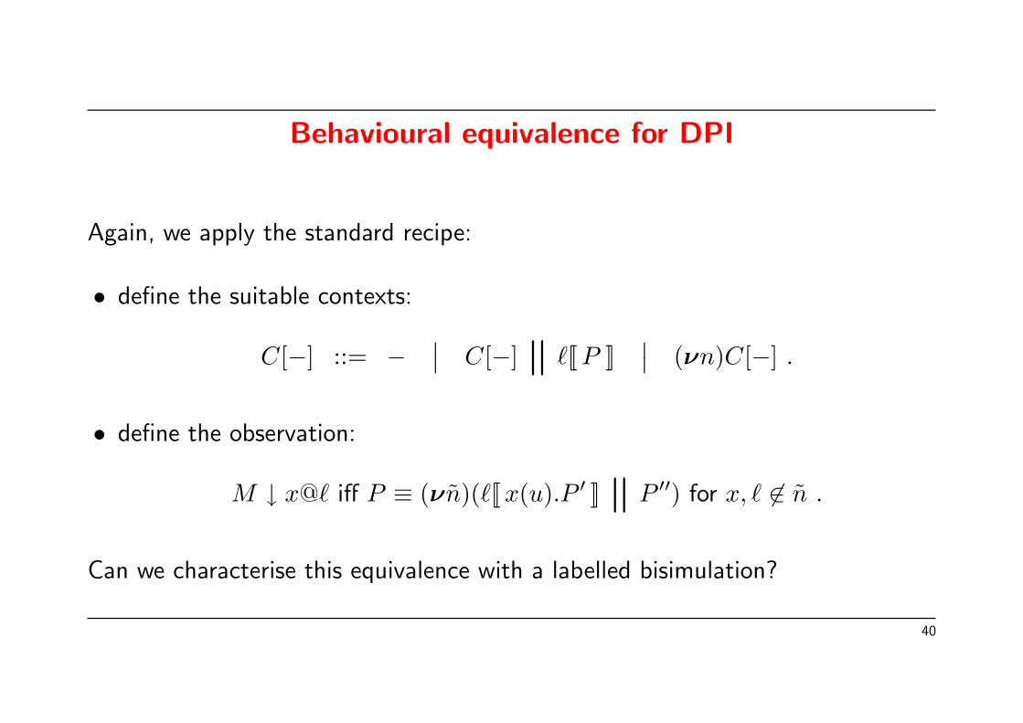
Behavioural equivalence for DPI

Again, we apply the standard recipe:

• define the suitable contexts:

C[−] ::= −∣∣ C[−]

n`[[ P ]]

∣∣ (νn)C[−] .

• define the observation:

M ↓ x@` iff P ≡ (νn)(`[[ x(u).P ′ ]]n

P ′′) for x, ` 6∈ n .

Can we characterise this equivalence with a labelled bisimulation?

40

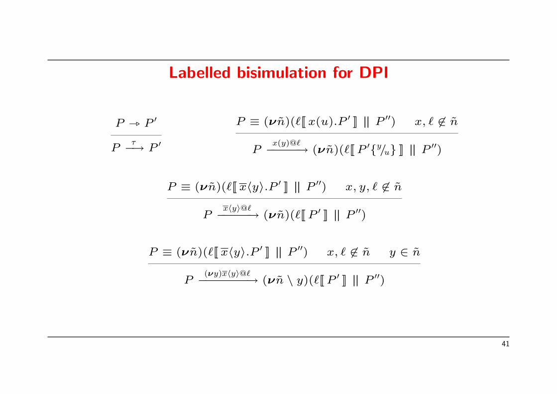
Labelled bisimulation for DPI

P _ P ′

Pτ−→ P ′

P ≡ (νn)(`[[ x(u).P ′ ]]f

P ′′) x, ` 6∈ n

Px(y)@`−−−−−→ (νn)(`[[ P ′y/u ]]

fP ′′)

P ≡ (νn)(`[[ x〈y〉.P ′ ]]f

P ′′) x, y, ` 6∈ n

Px〈y〉@`−−−−−→ (νn)(`[[ P ′ ]]

fP ′′)

P ≡ (νn)(`[[ x〈y〉.P ′ ]]f

P ′′) x, ` 6∈ n y ∈ n

P(νy)x〈y〉@`−−−−−−−→ (νn \ y)(`[[ P ′ ]]

fP ′′)

41

Labelled bisimulation for DPI, ctd.

The standard bisimulation on top of the LTS below coincides with reductionbarbed congruence.

Remark: the LTS is written in an unconventional style, which preciselycharacterises the interactions a term can have with a context.

Questions:

1- every label should correspond to a (minimal) interacting context: can you spellout these contexts?

2- why there are no explicit labels for the ”goto” action?

42

Mobile Ambients, design choices

Objective: build a process language on top of the concepts of barriers(administrative domains, firewalls, ...) and of barrier crossing.

A graphical representation of the syntax and of the reduction semantics of Mobile Ambients can

be found here:

http://research.microsoft.com/Users/luca/Slides/2000-11-10%20Wide%20Area%20Computation%20(Valladolid).pdf

43

Mobile Ambients syntax (in ISO 10646)

Processes: Capabilities:P,Q,R ::= 0 C ::= in n∣∣ P1

fP2

∣∣ out n∣∣ (νn)P∣∣ open n∣∣ n[P ]∣∣ C.P∣∣ !P

44

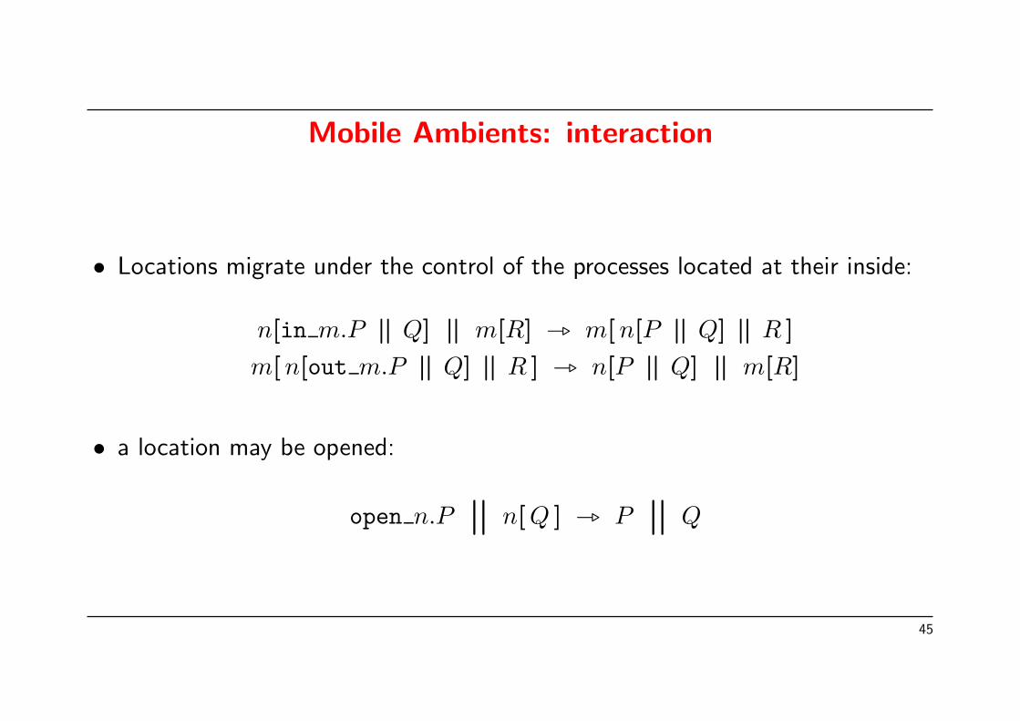
Mobile Ambients: interaction

• Locations migrate under the control of the processes located at their inside:

n[in m.Pf

Q]f

m[R] _ m[n[Pf

Q]f

R ]m[n[out m.P

fQ]

fR ] _ n[P

fQ]

fm[R]

• a location may be opened:

open n.Pn

n[Q ] _ Pn

Q

45

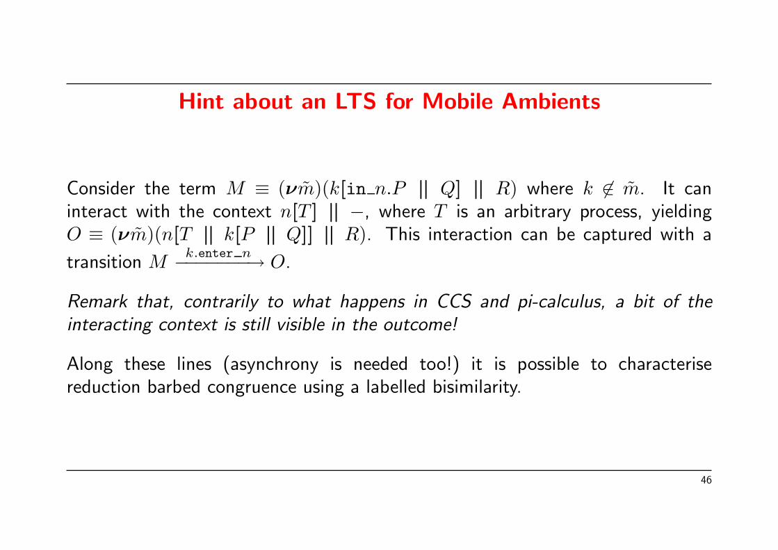
Hint about an LTS for Mobile Ambients

Consider the term M ≡ (νm)(k[in n.Pf

Q]f

R) where k 6∈ m. It caninteract with the context n[T ]

f−, where T is an arbitrary process, yielding

O ≡ (νm)(n[Tf

k[Pf

Q]]f

R). This interaction can be captured with a

transition Mk.enter n−−−−−−−→ O.

Remark that, contrarily to what happens in CCS and pi-calculus, a bit of theinteracting context is still visible in the outcome!

Along these lines (asynchrony is needed too!) it is possible to characterisereduction barbed congruence using a labelled bisimilarity.

46

References

James Riely, Matthew Hennessy: Distributed Pprocesses and location failures.Theoretical Computer Science, 2001. An extended abstract appeard in ICALP 97.

Luca Cardelli, Andrew Gordon: Mobile Ambients. Theoretical Computer Science,2000. An extended abstract appeared in FOSSACS 1998.

47

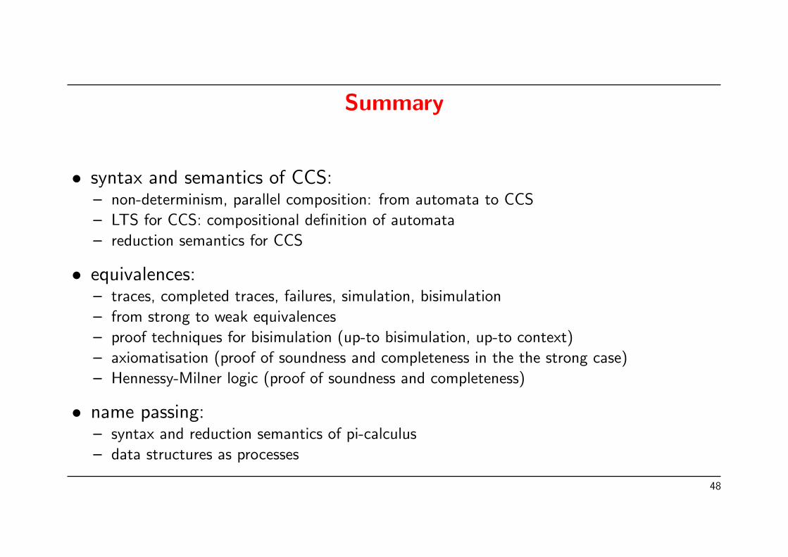
Summary

• syntax and semantics of CCS:– non-determinism, parallel composition: from automata to CCS

– LTS for CCS: compositional definition of automata

– reduction semantics for CCS

• equivalences:– traces, completed traces, failures, simulation, bisimulation

– from strong to weak equivalences

– proof techniques for bisimulation (up-to bisimulation, up-to context)

– axiomatisation (proof of soundness and completeness in the the strong case)

– Hennessy-Milner logic (proof of soundness and completeness)

• name passing:– syntax and reduction semantics of pi-calculus

– data structures as processes

48

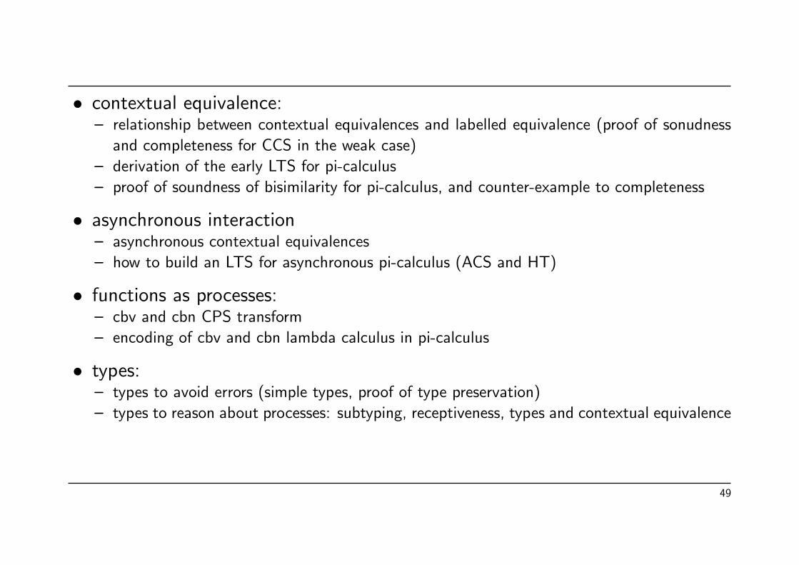
• contextual equivalence:– relationship between contextual equivalences and labelled equivalence (proof of sonudness

and completeness for CCS in the weak case)

– derivation of the early LTS for pi-calculus

– proof of soundness of bisimilarity for pi-calculus, and counter-example to completeness

• asynchronous interaction– asynchronous contextual equivalences

– how to build an LTS for asynchronous pi-calculus (ACS and HT)

• functions as processes:– cbv and cbn CPS transform

– encoding of cbv and cbn lambda calculus in pi-calculus

• types:– types to avoid errors (simple types, proof of type preservation)

– types to reason about processes: subtyping, receptiveness, types and contextual equivalence

49

Partiel

20/11/07 — 12h45-15h45

Salle 1C12 — Chevaleret

Personal notes and lecture notes authorised.

50

Thank you for your attention

Feel free to contact me if you want to know more about research in concurrency.

francesco.zappa_nardelli@inria.fr

51