Fracture Design

Hydraulic FracturingHydraulic FracturingShort Course,Short Course,

Texas A&M UniversityTexas A&M UniversityCollege StationCollege Station

20052005

Fracture DesignFracture Design Fracture Dimensions Fracture Dimensions

Fracture Modeling Fracture Modeling

Peter P. ValkóPeter P. Valkó

Hydraulic FracturingHydraulic FracturingShort Course,Short Course,

Texas A&M UniversityTexas A&M UniversityCollege StationCollege Station

20052005

Fracture DesignFracture Design Fracture Dimensions Fracture Dimensions

Fracture Modeling Fracture Modeling

Peter P. ValkóPeter P. Valkó

FractureDesign

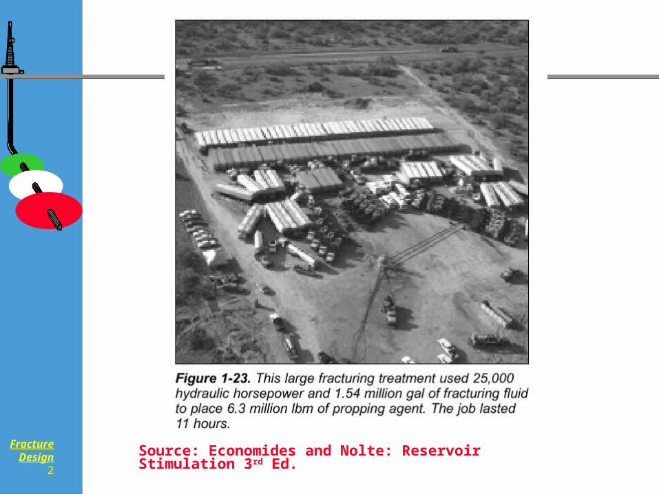
2Source: Economides and Nolte: Reservoir Stimulation 3rd Ed.

FractureDesign

3

Frac Design Goals

FractureDesign

4

Well or Reservoir Stimulation?

Near wellbore region and/or bulk reservoir?

Acceleration versus increasing reserve?

Low permeability

Medium permeability

High permeability

Coupling of goals

Frac&pack

FractureDesign

5

Hydraulic Fracturing Design and Evaluation

Why do we create a propped fracture?

How do we achieve our goals?

Data gathering

Design

Execution

Evaluation

FractureDesign

6

Fractured Well Performance

Relation of morphology to performance

Streamline view

Flow regimes, Productivity Index, Pseudo-

steady state Productivity Index, skin and

equivalent wellbore radius

FractureDesign

7

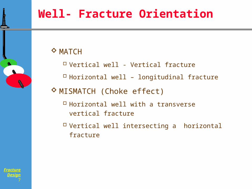
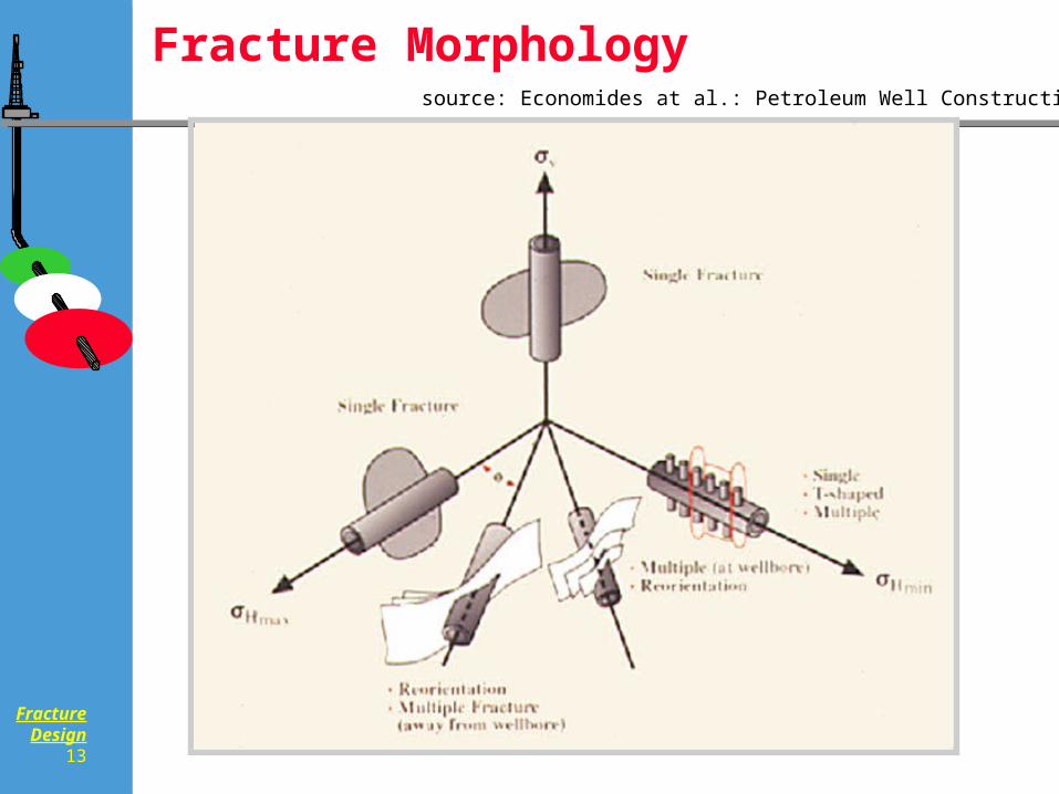
Well- Fracture Orientation

MATCH

Vertical well - Vertical fracture

Horizontal well – longitudinal fracture

MISMATCH (Choke effect)

Horizontal well with a transverse vertical fracture

Vertical well intersecting a horizontal fracture

FractureDesign

8

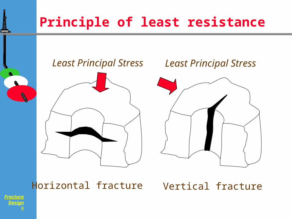
Principle of least resistance

Horizontal fracture Vertical fracture

Least Principal Stress Least Principal Stress

FractureDesign

9

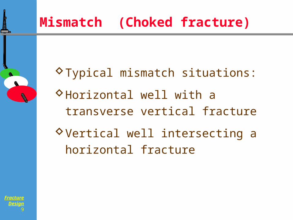
Mismatch (Choked fracture)

Typical mismatch situations:

Horizontal well with a transverse vertical

fracture

Vertical well intersecting a horizontal

fracture

FractureDesign

10

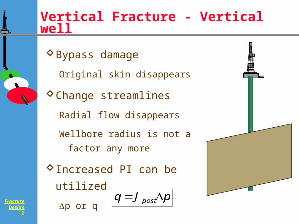
Vertical Fracture - Vertical well

Bypass damage

Original skin disappears

Change streamlines

Radial flow disappears

Wellbore radius is not a factor

any more

Increased PI can be utilized

p or q pJq post

FractureDesign

11

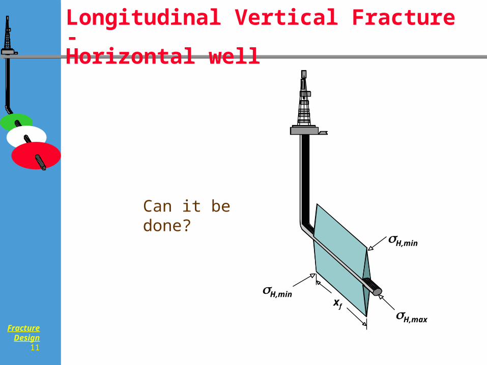
Longitudinal Vertical Fracture -Horizontal well

H,maxxf

H,min

H,min

Can it be done?

FractureDesign

12

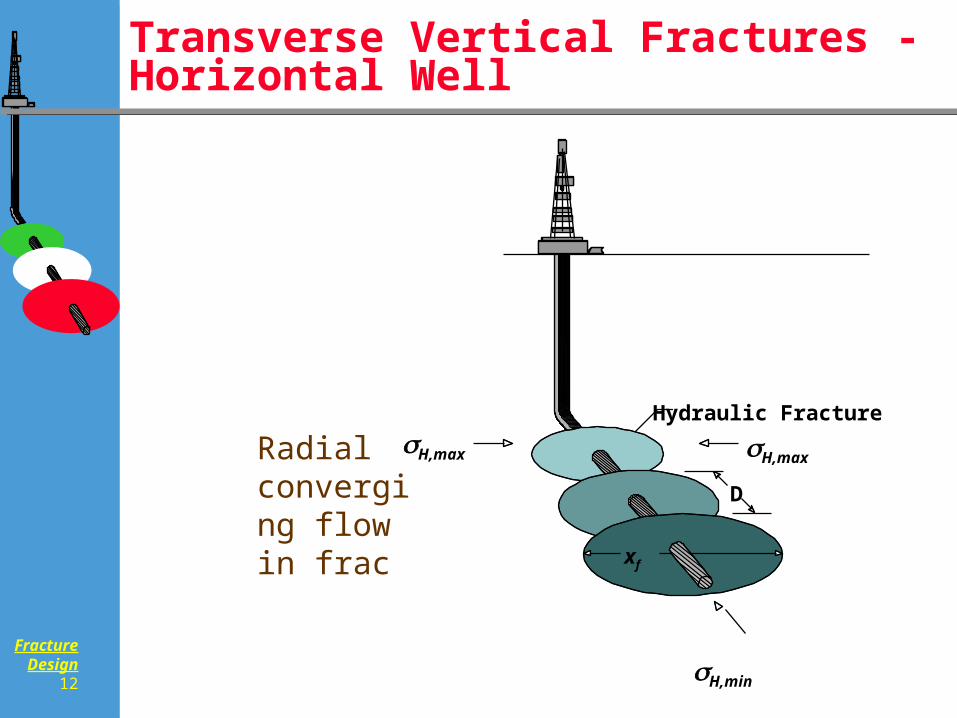
Transverse Vertical Fractures - Horizontal Well

H,maxHydraulic Fracture

H,maxD

xf

H,min

Radial converging flow in frac

FractureDesign

13

Fracture Morphologysource: Economides at al.: Petroleum Well Construction

FractureDesign

14

Main questions

Which wellbore-fracture orientation is favorable?

Which can be done?

How large should the treatment be?

What part of the proppant will reach the pay?

Width and length (optimum dimensions)?

How can it be realized?

FractureDesign

15

Prod Eng 101

Transient vs Pseudo-steady state

Productivity Index

Skin

FractureDesign

16

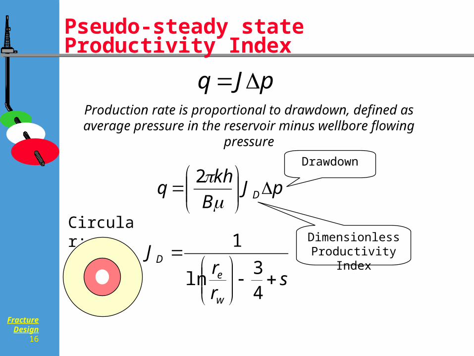
Pseudo-steady state Productivity Index

pJq

pJB

khq D

2

srr

J

w

e

D

43

ln

1Circular:

Production rate is proportional to drawdown, defined as average pressure in the reservoir minus wellbore flowing pressure

Dimensionless Productivity Index

Drawdown

FractureDesign

17

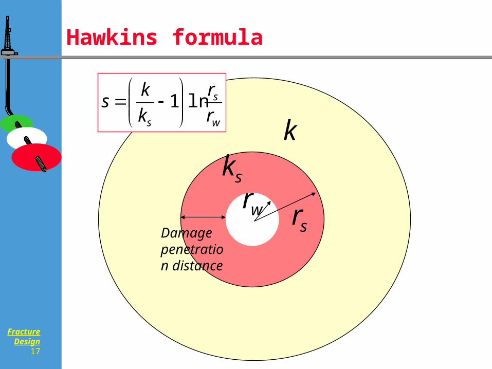
Hawkins formula

w

s

s r

r

k

ks ln1

skk

wrsrDamage

penetration distance

FractureDesign

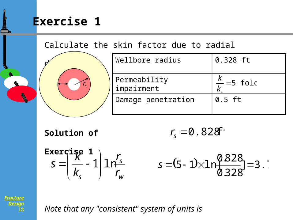
18

Calculate the skin factor due to radial damage if

Solution of Exercise 1

w

s

s r

r

k

ks ln1

0.5 ftDamage penetration

Permeability impairment

0.328 ftWellbore radius

folds 5sk

k

ft 0.828sr

Note that any "consistent" system of units is OK.

sr

3.7]328.0

828.0ln[15 s

Exercise 1

FractureDesign

19

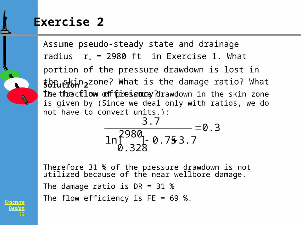
Assume pseudo-steady state and drainage radius re = 2980 ft in

Exercise 1. What portion of the pressure drawdown is lost in the

skin zone? What is the damage ratio? What is the flow efficiency?

Solution 2The fraction of pressure drawdown in the skin zone is given by (Since we deal only with ratios, we do not have to convert units.):

Therefore 31 % of the pressure drawdown is not utilized because of the near wellbore damage.

The damage ratio is DR = 31 %

The flow efficiency is FE = 69 %.

0.313.70.75]

0.3282980

ln[

3.7

Exercise 2

FractureDesign

20

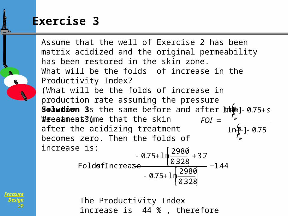
Assume that the well of Exercise 2 has been matrix acidized and the original permeability has been restored in the skin zone. What will be the folds of increase in the Productivity Index?(What will be the folds of increase in production rate assuming the pressure drawdown is the same before and after the treatment?)

Solution 3We can assume that the skin after the acidizing treatment becomes zero. Then the folds of increase is:

75.0]ln[

75.0]ln[

w

e

w

e

rr

srr

FOI

44.1

328.02980

ln75.0

7.3328.0

2980ln75.0

:Increase of Folds

The Productivity Index increase is 44 % , therefore the production increase is 44 % .

Exercise 3

FractureDesign

21

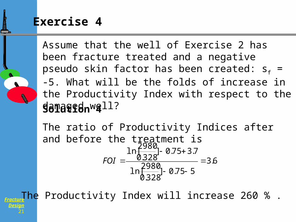
Assume that the well of Exercise 2 has been fracture treated and a negative pseudo skin factor has been created: sf = -5. What will be the folds of increase in the Productivity Index with respect to the damaged well?

6.3575.0]

328.02980

ln[

7.375.0]328.0

2980ln[

FOI

Solution 4

The ratio of Productivity Indices after and before the treatment is

The Productivity Index will increase 260 % .

Exercise 4

FractureDesign

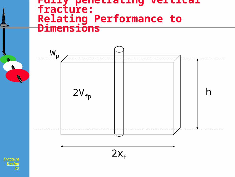
22

Fully penetrating vertical fracture: Relating Performance to Dimensions

wp

2xf

h2Vfp

FractureDesign

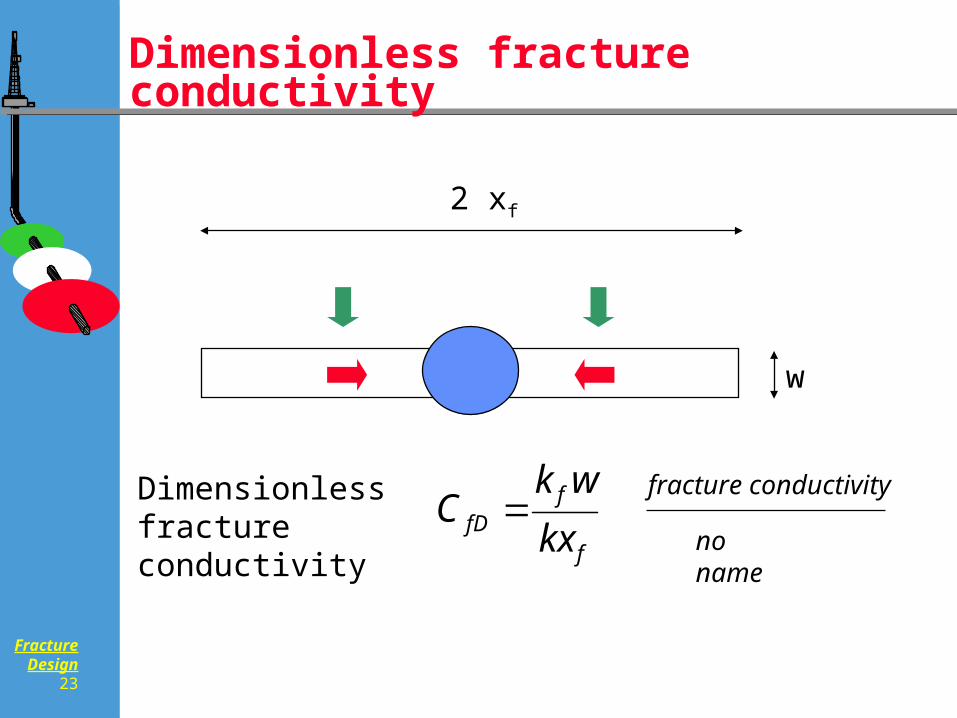
23

Dimensionless fracture conductivity

Dimensionless fracture conductivity

f

ffD kx

wkC

2 xf

w

fracture conductivity

no name

FractureDesign

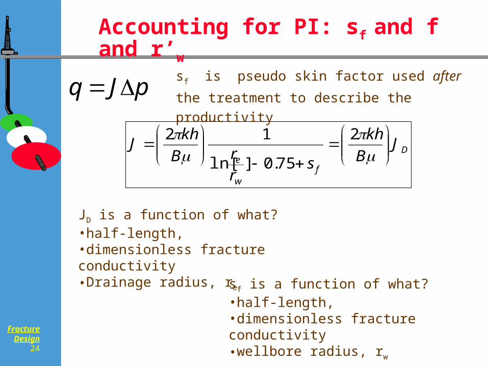
24

Accounting for PI: sf and f and r’w

D

fw

e

JB

kh

sr

rB

khJ

2

75.0]ln[

12

q J p

sf is a function of what?•half-length, •dimensionless fracture conductivity•wellbore radius, rw

JD is a function of what?•half-length, •dimensionless fracture conductivity•Drainage radius, re

sf is pseudo skin factor used after the treatment

to describe the productivity

FractureDesign

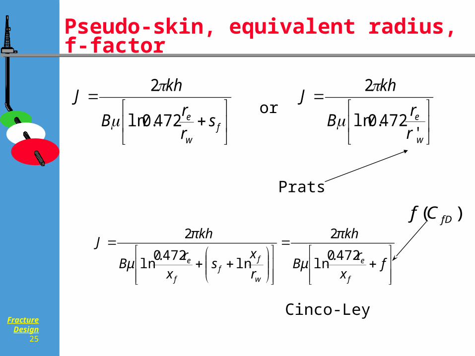
25

Pseudo-skin, equivalent radius, f-factor

)( fDCf

or

Prats

Cinco-Ley

w

e

r

rB

khJ

'472.0ln

2

fw

e srr

B

khJ

472.0ln

2

fx

r.Bμ

πkh

r

xs

x

r.Bμ

πkhJ

f

e

w

ff

f

e 4720ln

2

ln4720

ln

2

FractureDesign

26

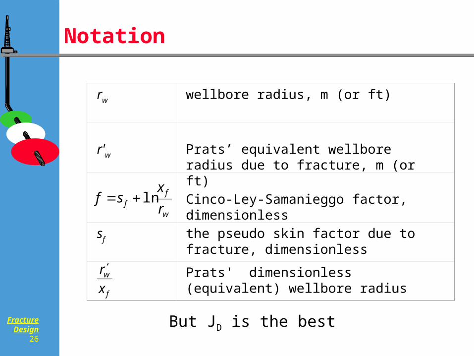
Notation

rw wellbore radius, m (or ft)

r'w Prats’ equivalent wellbore radius due to fracture, m (or ft)

Cinco-Ley-Samanieggo factor, dimensionless

sf the pseudo skin factor due to fracture, dimensionless

Prats' dimensionless (equivalent) wellbore radiusf

w

x

r

w

ff r

xsf ln

But JD is the best

FractureDesign

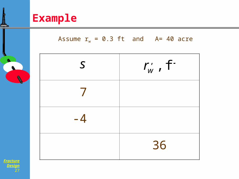
27

7

-4

36

Example

Assume rw = 0.3 ft and A= 40 acre

ft , ,wrs

FractureDesign

28

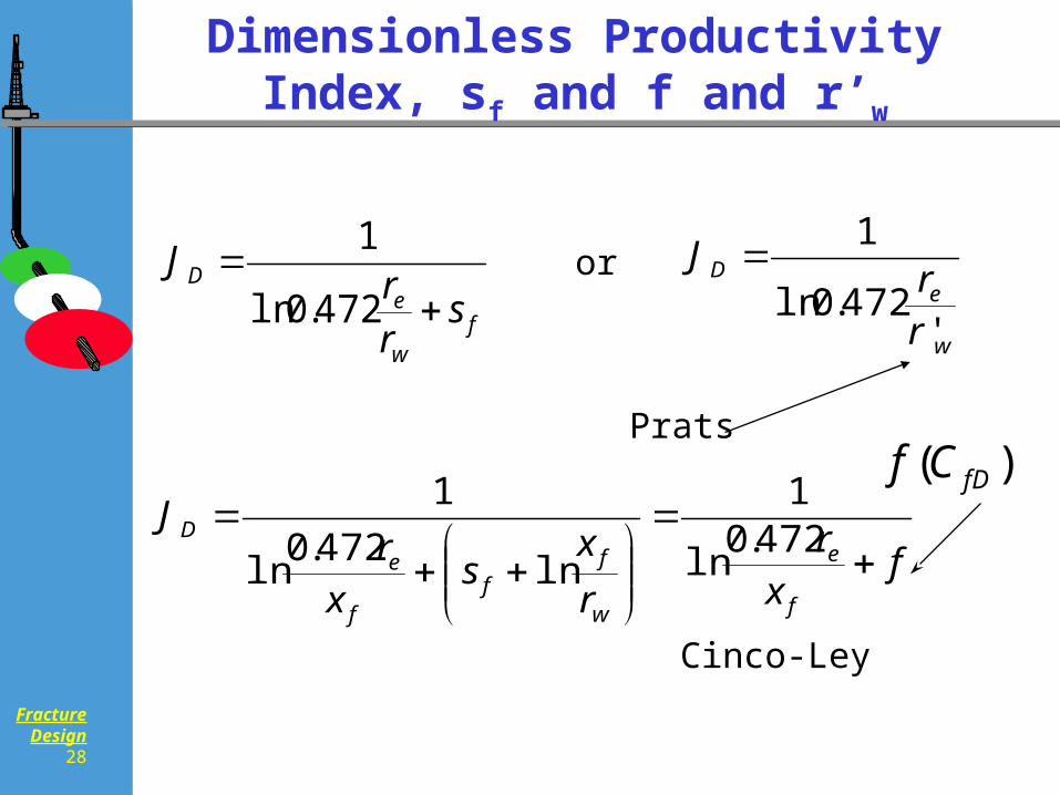
Dimensionless Productivity Index, sf and f and r’w

fx

r

r

xs

xr

J

f

e

w

ff

f

e

D

472.0

ln

1

ln472.0

ln

1

fw

eD

sr

rJ

472.0ln

1

)( fDCf

w

eD

rr

J

'472.0ln

1or

Prats

Cinco-Ley

FractureDesign

29

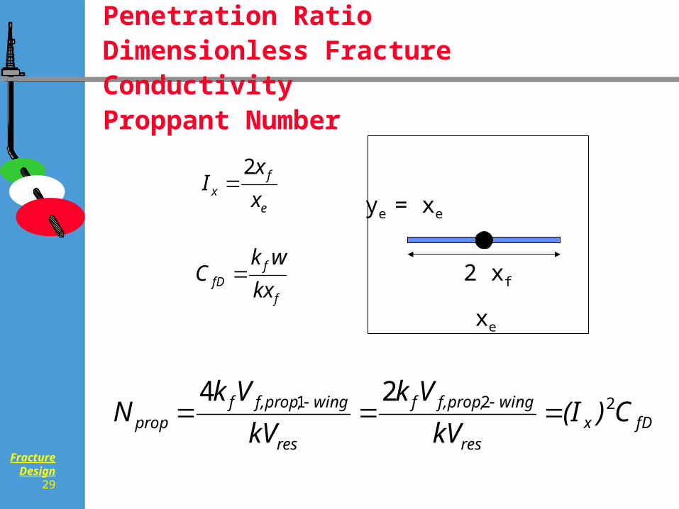
Penetration Ratio Dimensionless Fracture ConductivityProppant Number

2 xf

ye = xe

xe

e

fx x

xI

2

f

ffD kx

wkC

fDxres

wingf,prop,f

res

wingf,prop,fprop C)(I

kV

Vk

kV

VkN 221 24

FractureDesign

30

The following models, graphs and correlations are valid for low to moderate Proppant Number, Nprop

OK, so what IS the Proppant Number?

The weighted ratio of propped fracture volume to reservoir volume. The weight is 2kf/k .

A more rigorous definition will be given later.

The following models are valid for Nprop <=0.1 ! (The

case when the boundaries do not distort the streamline structure (with respect to lower proppant numbers.)

FractureDesign

31

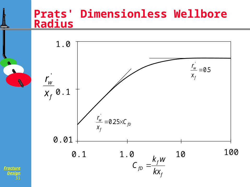
Prats' Dimensionless Wellbore Radius

f

w

x

r '

f

ffD kx

wkC

0.01

0.1

1.0

0.1 1.0 10 100

5.0'

f

w

x

r

fDf

w Cx

r 25.0

'

FractureDesign

32

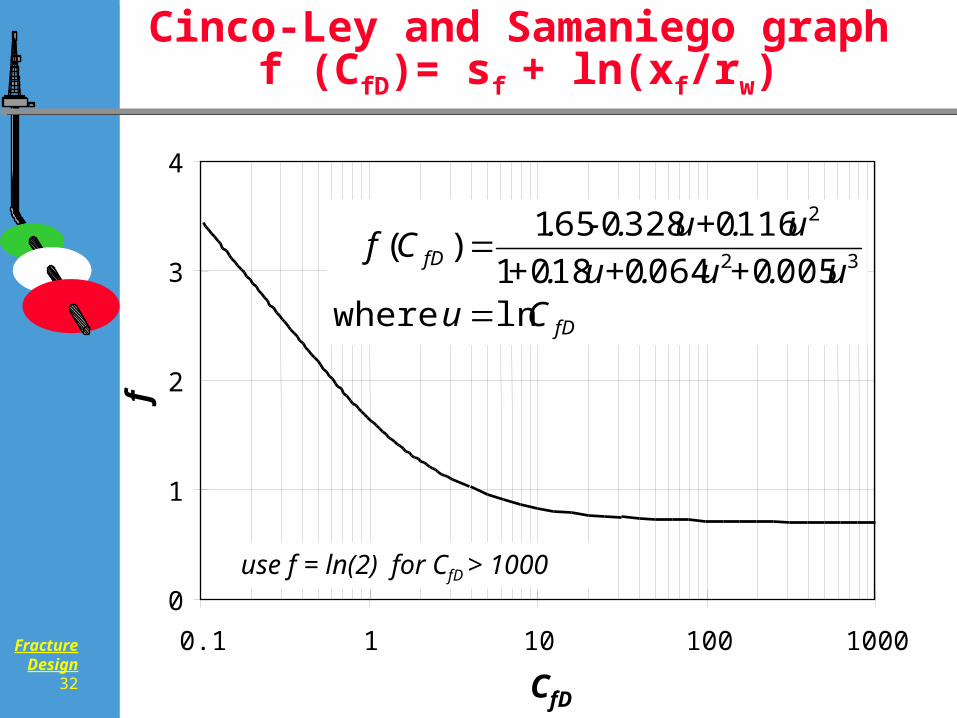
Cinco-Ley and Samaniego graphf (CfD)= sf + ln(xf/rw)

0

1

2

3

4

0.1 1 10 100 1000

CfD

f

fD

fD

Cuu.+u.u+.+

u.u+.-.Cf

ln where005006401801

11603280651)(

32

2

use f = ln(2) for CfD > 1000

FractureDesign

33

Infinite or finite conductivity fracture

Note that after CfD > 100 (or 30), nothing happens

with f.

Infinite conductivity fracture.

Definition: finite conductivity fracture is a not infinite

conductivity fracture (CfD < 100 or 30)

(Other concept: uniform flux fracture, we will learn

later.)

FractureDesign

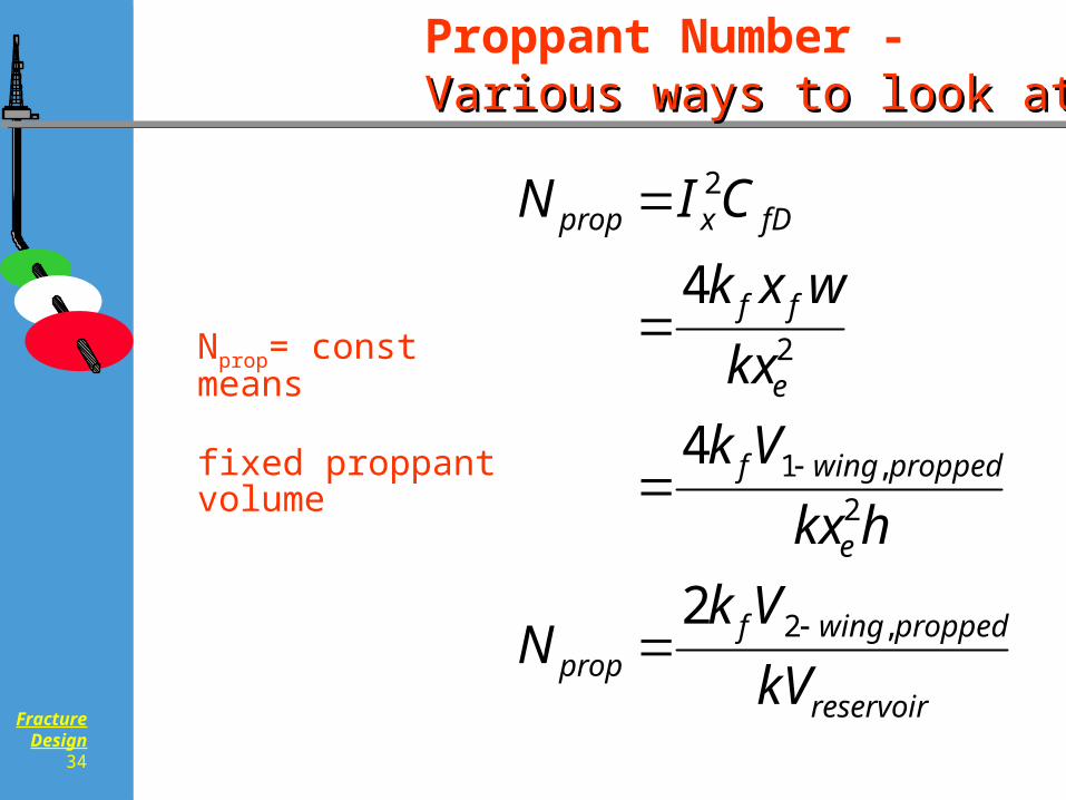
34

reservoir

proppedwingfprop

e

proppedwingf

e

ff

fDxprop

kV

VkN

hkx

Vk

kx

wxk

CIN

,2

2

,1

2

2

2

4

4

Proppant Number - Various ways to look at itVarious ways to look at it

Nprop= const means

fixed proppant volume

FractureDesign

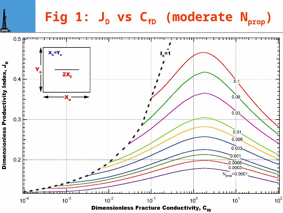
35

Fig 1: JD vs CfD (moderate Nprop)

FractureDesign

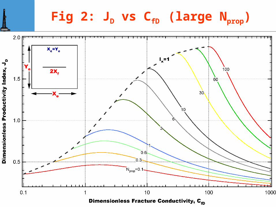
36

Fig 2: JD vs CfD (large Nprop)

FractureDesign

37

OPTIMIZATION

FractureDesign

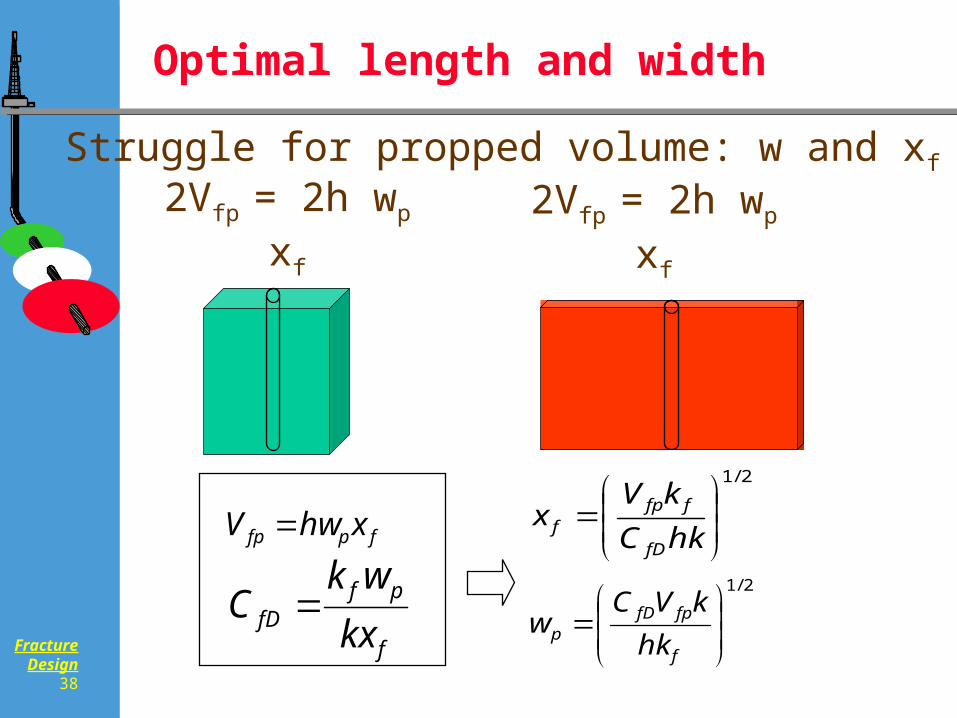
38

Optimal length and width

2Vfp = 2h wp xf

Struggle for propped volume: w and xf

fpfp xhwV

f

pffD kx

wkC

2/1

hkC

kVx

fD

ffpf

2/1

f

fpfDp hk

kVCw

2Vfp = 2h wp xf

FractureDesign

39

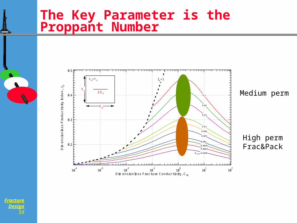
The Key Parameter is the Proppant Number

0.5

0.4

0.3

0.2

Dim

en

sio

nle

ss P

rod

uc

tivit

y I

nd

ex

, J

D

10-4

10-3

10-2

10-1

100

101

102

Dimensionless Frac ture Conduc tivity, C fD

0.001

0.003

0.006

N prop=0.0001

0.01

0.03

0.06

0.0003

0.0006

I x=1

Xe

2X f

Y e

X e=Y e

0.1

High permFrac&Pack

Medium perm

FractureDesign

40

2.0

1.5

1.0

0.5Dim

en

sio

nle

ss P

rod

uc

tivit

y I

nd

ex

, J

D

0.1 1 10 100 1000

Dimensionless Frac ture Conduc tivity, C fD

N prop=0.1

0.3

0.6

1

3

6

10

30

60

100

Xe

2X f

Y e

X e=Y e

I x=1

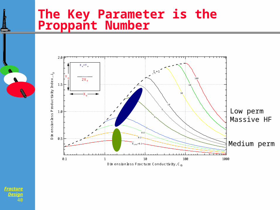
The Key Parameter is the Proppant Number

Low permMassive HF

Medium perm

FractureDesign

41

Let us read the optimum from the JD

Figures!

dimensionless fracture conductivity

(for smaller Nprop)

penetration ratio

(for larger Nprop)

FractureDesign

42

0.5

0.4

0.3

0.2

Dim

en

sio

nle

ss P

rod

uc

tivi

ty I

nd

ex

, JD

10-4

10-3

10-2

10-1

100

101

102

Dimensionless Frac ture Conduc tivity, C fD

0.001

0.003

0.006

N prop=0.0001

0.01

0.03

0.06

0.0003

0.0006

I x=1

Xe

2X f

Y e

X e=Y e

0.1

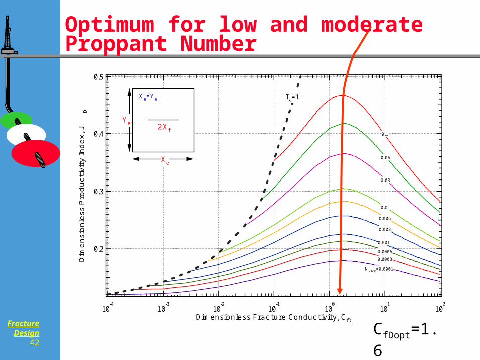
CfDopt=1.6

Optimum for low and moderate Proppant Number

FractureDesign

43

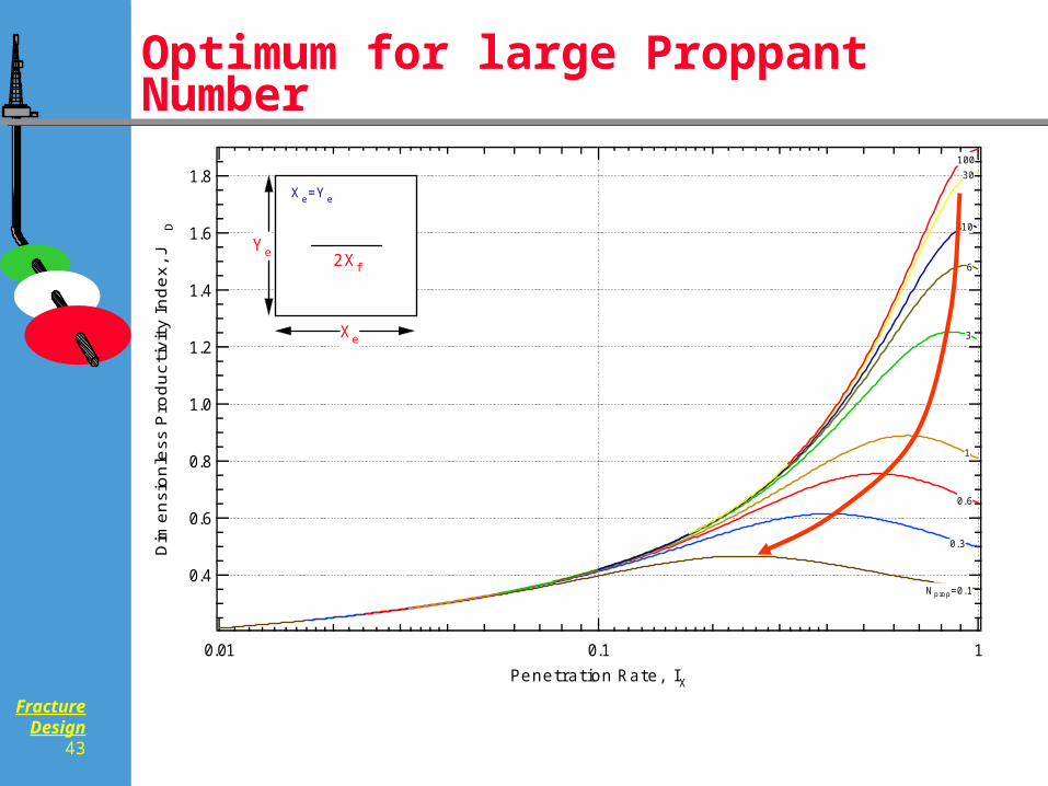
1.8

1.6

1.4

1.2

1.0

0.8

0.6

0.4

Dim

en

sio

nle

ss P

rod

uc

tivi

ty I

nd

ex

, JD

0.01 0.1 1

Penetration Rate, IX

N prop=0.1

0.3

0.6

1

3

6

10

30

100

Xe

2X f

Y e

X e=Y e

Optimum for large Proppant Number

FractureDesign

44

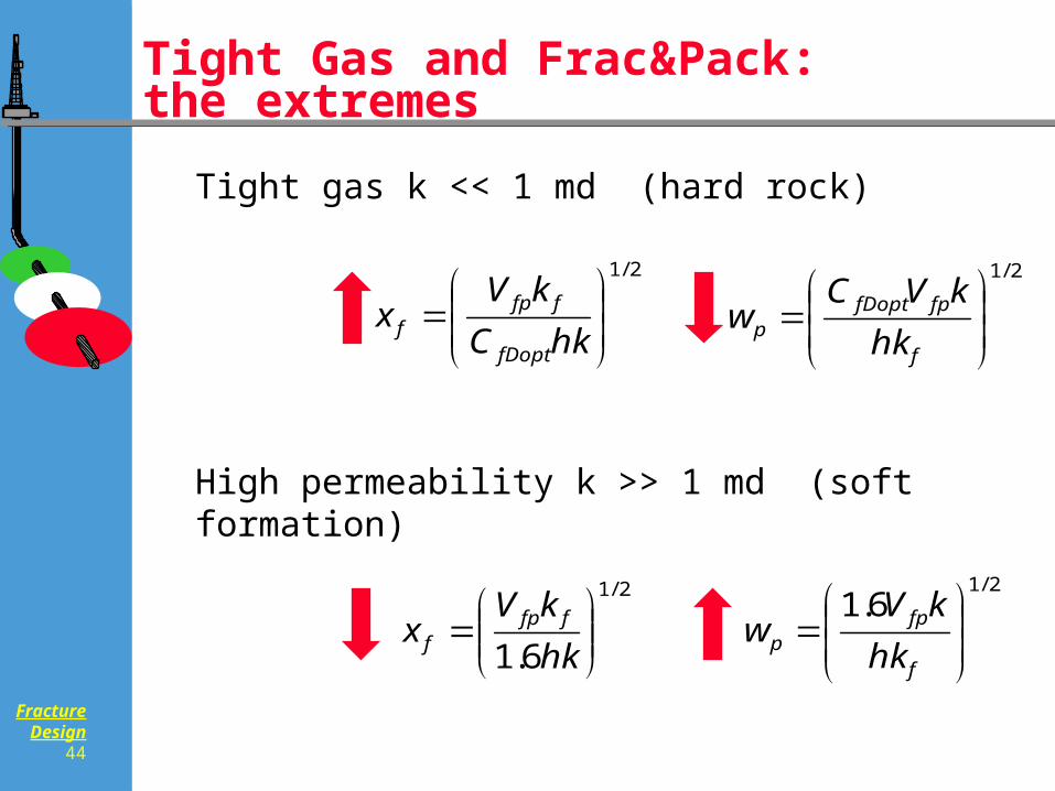
Tight Gas and Frac&Pack: the extremes

Tight gas k << 1 md (hard rock)

High permeability k >> 1 md (soft formation)

2/1

f

fpfDoptp hk

kVCw

2/1

hkC

kVx

fDopt

ffpf

2/16.1

f

fpp hk

kVw

2/1

6.1

hk

kVx ffp

f

FractureDesign

45

FracPi

FractureDesign

46

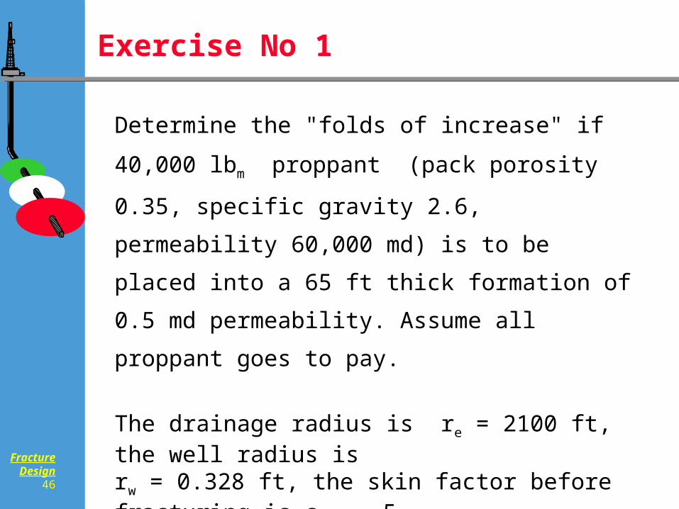
Exercise No 1

Determine the "folds of increase" if 40,000 lbm proppant

(pack porosity 0.35, specific gravity 2.6, permeability

60,000 md) is to be placed into a 65 ft thick formation of

0.5 md permeability. Assume all proppant goes to pay.

The drainage radius is re = 2100 ft, the well radius is rw = 0.328 ft, the skin factor before fracturing is spre = 5.

Determine the optimal fracture length and propped

width.

FractureDesign

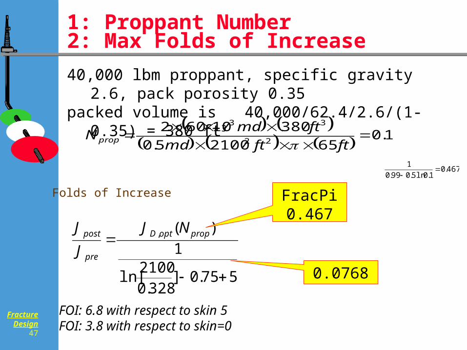
47

575.0]328.0

2100ln[

1

)(,

propoptD

pre

post NJ

J

J

Folds of Increase

40,000 lbm proppant, specific gravity 2.6, pack porosity 0.35packed volume is 40,000/62.4/2.6/(1-0.35) = 380 ft3

1: Proppant Number 2: Max Folds of Increase

FracPi0.467

1.0

6521005.0

3801060222

33

ftftmd

ftmdN prop

0.0768

FOI: 6.8 with respect to skin 5FOI: 3.8 with respect to skin=0

467.01.0ln5.099.0

1

FractureDesign

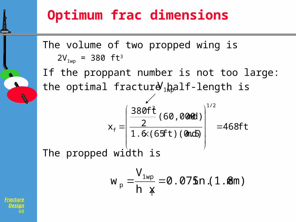
48

The volume of two propped wing is 2V1wp = 380 ft3

If the proppant number is not too large: the optimal fracture

half-length is

The propped width is

Optimum frac dimensions

mm) (1.8 in. 0.075h x

Vw

f

1wpp

ft 468 md) ft)(0.5 (651.6

md) (60,000 2

ft 380

x

1/23

f

1wpV

FractureDesign

49

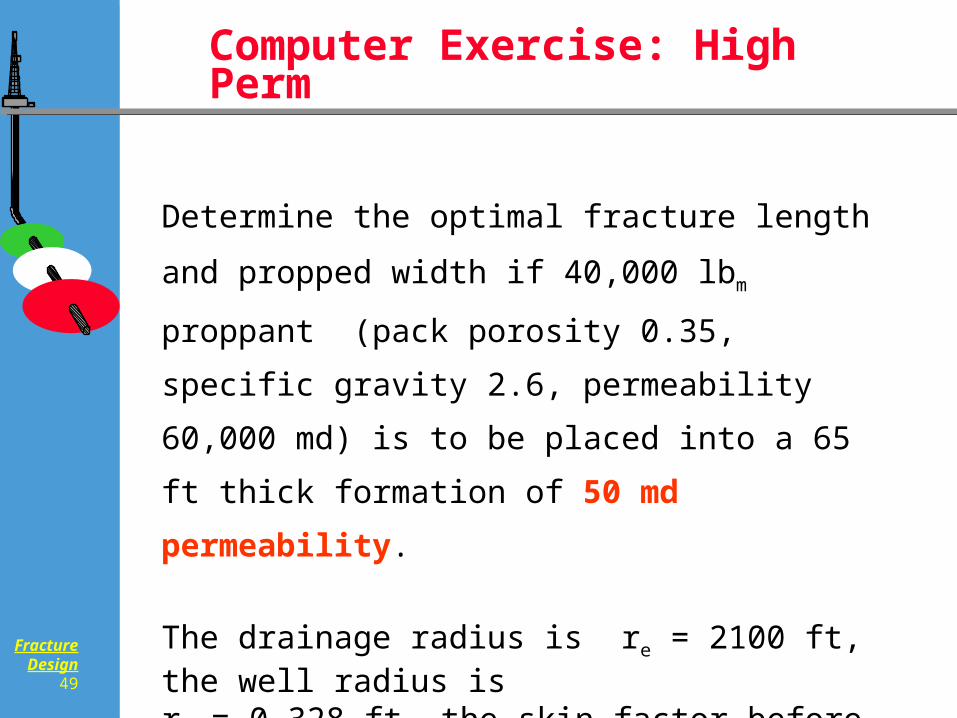
Computer Exercise: High Perm

Determine the optimal fracture length and propped width

if 40,000 lbm proppant (pack porosity 0.35, specific

gravity 2.6, permeability 60,000 md) is to be placed into

a 65 ft thick formation of 50 md permeability.

The drainage radius is re = 2100 ft, the well radius is rw = 0.328 ft, the skin factor before fracturing is spre = 5.

(Assume all proppant goes to pay.)

FractureDesign

50

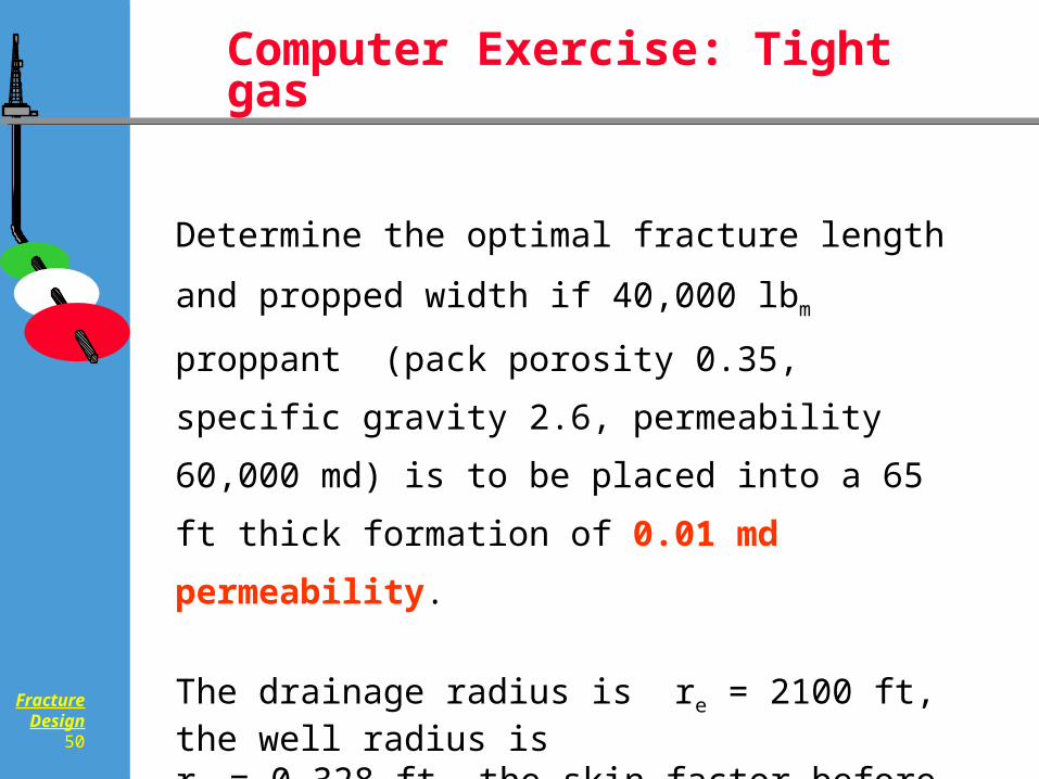
Computer Exercise: Tight gas

Determine the optimal fracture length and propped width

if 40,000 lbm proppant (pack porosity 0.35, specific

gravity 2.6, permeability 60,000 md) is to be placed into

a 65 ft thick formation of 0.01 md permeability.

The drainage radius is re = 2100 ft, the well radius is rw = 0.328 ft, the skin factor before fracturing is spre = 5.

(Assume all proppant goes to pay.)

FractureDesign

51

Economic optimization

Production forecast

Transient regime

Stabilized

Economics: Converting additional production into value

Time value of money

Discounted revenue

NPV

FractureDesign

52

Costs and Benefits

The more proppant (larger proppant

number) the higher Productivity Index, if

the given proppant volume is placed

according to the optimal dimensionless

fracture conductivity

The more proppant, the larger costs

How large should be the treatment?

NPV optimization

FractureDesign

53

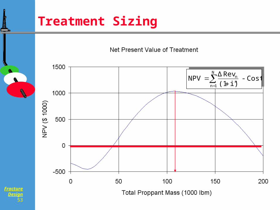
Treatment Sizing

Cost - i)(1

RevΔNPV

N

1nnn

Cost -

i)(1

RevΔNPV

N

1nnn

FractureDesign

54

Pre-Treatment Data Gathering

FractureDesign

55

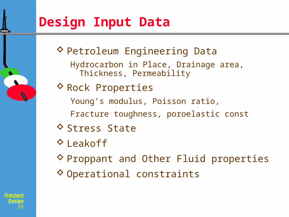
Design Input Data

Petroleum Engineering DataHydrocarbon in Place, Drainage area, Thickness,

Permeability

Rock PropertiesYoung’s modulus, Poisson ratio,

Fracture toughness, poroelastic const

Stress State

Leakoff

Proppant and Other Fluid properties

Operational constraints

FractureDesign

56

Rock Properties

Linear Elasticity

Poroelasticity

Fracture Mechanics

FractureDesign

57

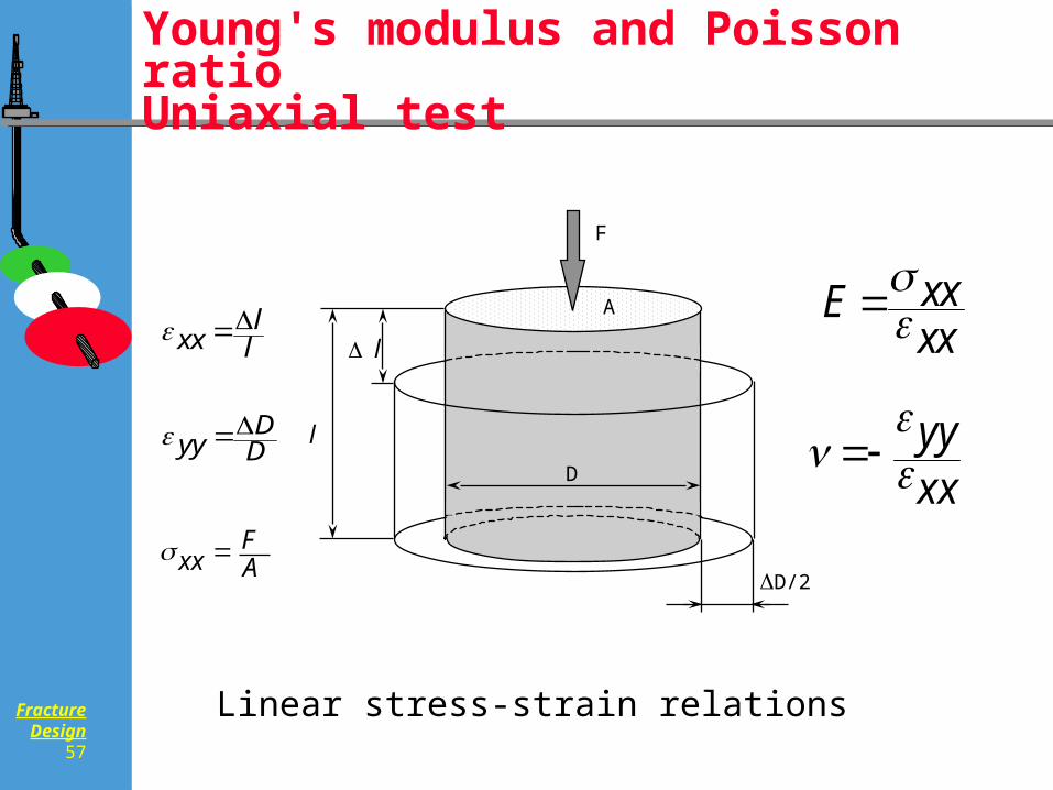
Young's modulus and Poisson ratioUniaxial test

xxFA

xxl

l

yyD

D

D

D/2

l

l

F

A E xxxx

xxyy

Linear stress-strain relations

FractureDesign

58

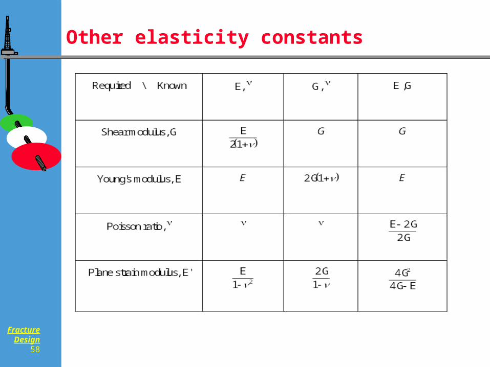
Other elasticity constants

FractureDesign

59

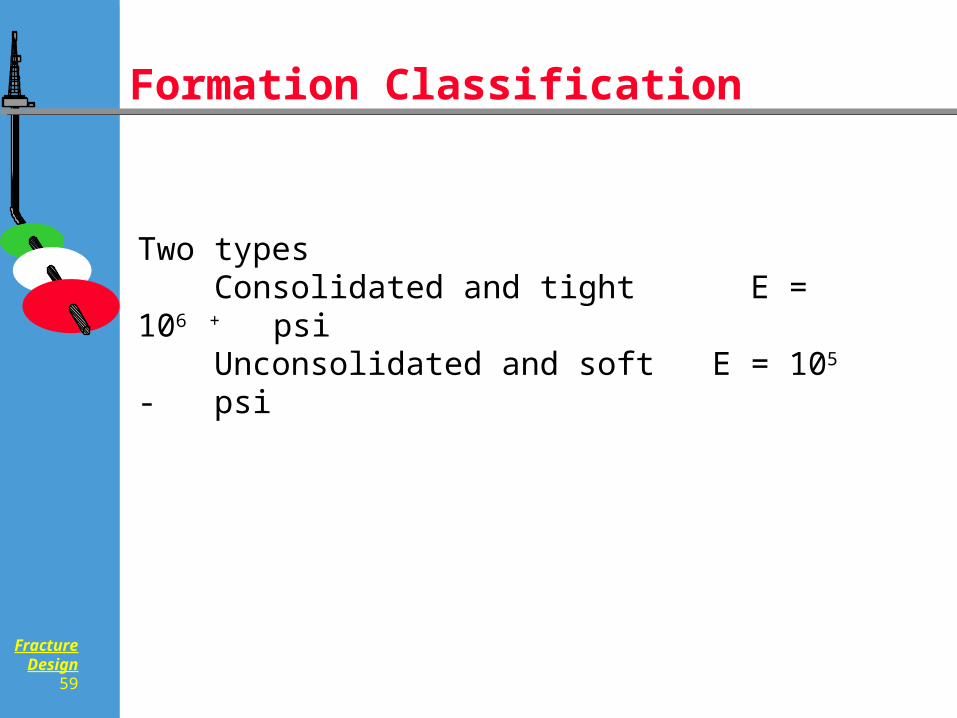
Formation Classification

Two types Consolidated and tight E = 106 + psi Unconsolidated and soft E = 105 - psi

FractureDesign

60

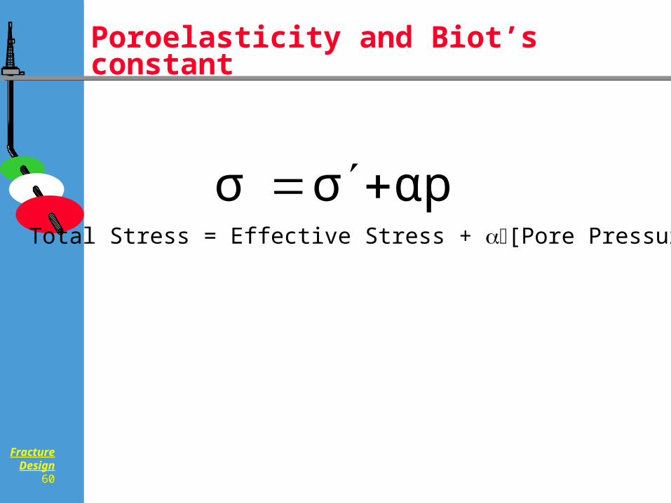
Poroelasticity and Biot’s constant

αpσ σ Total Stress = Effective Stress + [Pore Pressure]

FractureDesign

61

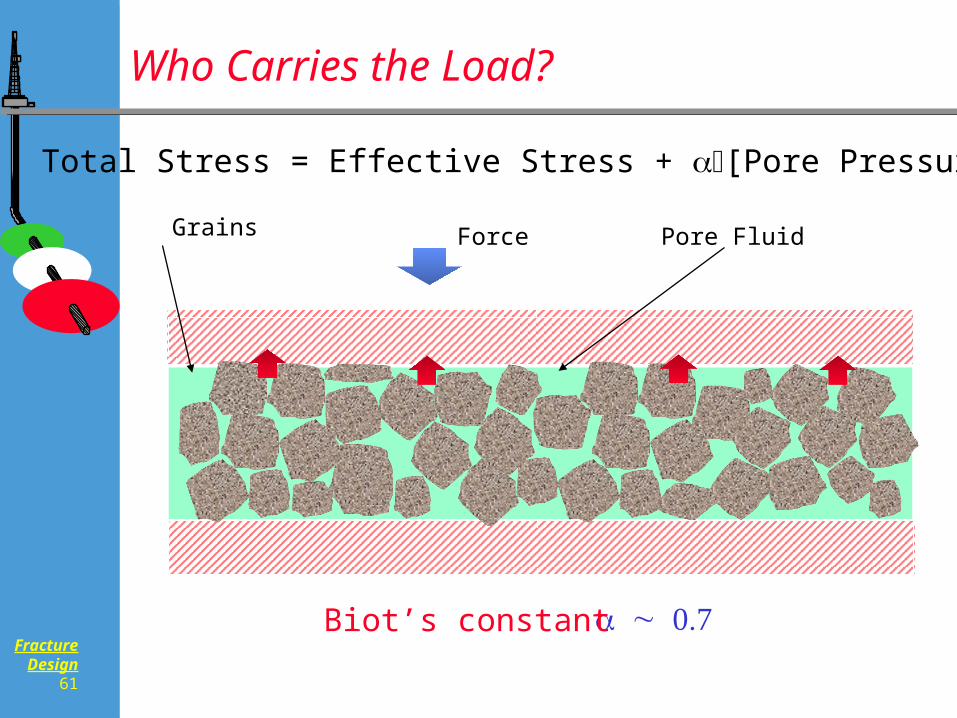
Who Carries the Load?

Force Pore FluidGrains

Biot’s constant

Total Stress = Effective Stress + [Pore Pressure]

FractureDesign

62

Stress State in Formations Far Field and Induced Stresses, Fracture Initiation and Orientation

Stress versus Depth

Minimum Horizontal Stress

Magnitude and Direction

FractureDesign

63

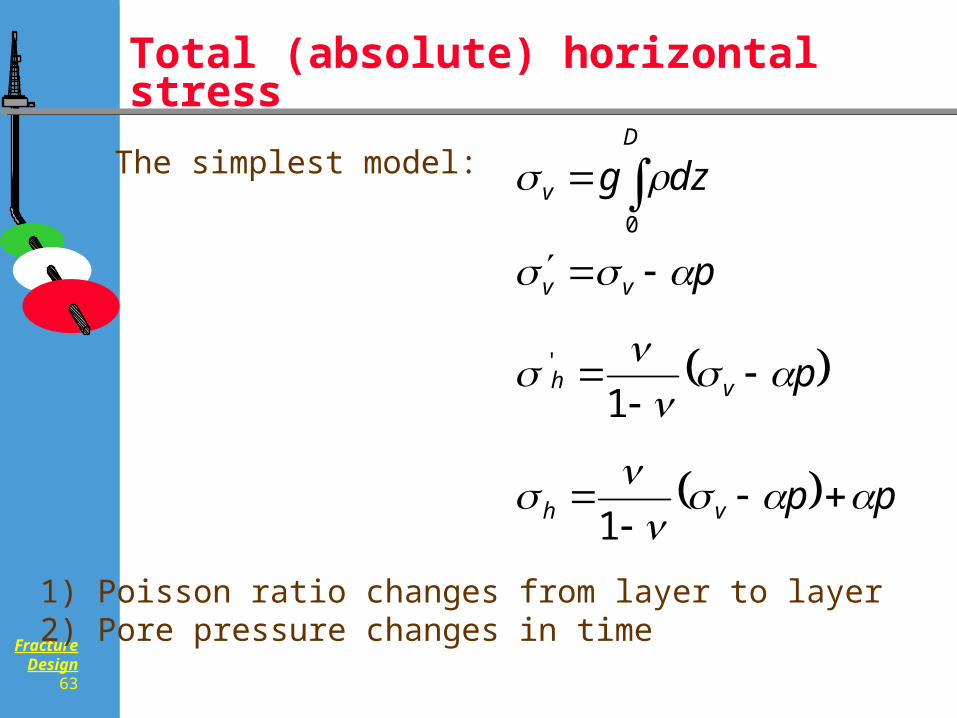
Total (absolute) horizontal stress

D

v dzg0

pvv

pvh

1

'

ppvh

1

The simplest model:

1) Poisson ratio changes from layer to layer2) Pore pressure changes in time

FractureDesign

64

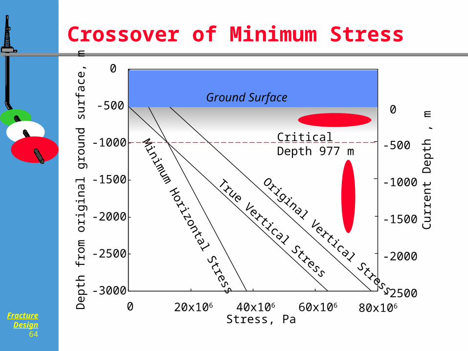
Crossover of Minimum Stress

80x1060 20x106 40x106 60x106

Stress, Pa

Dep

th f

rom

orig

inal

gro

und

surf

ace,

m

Original Vertical Stress

True Vertical Stress

Minim

um H

orizontal Stress

Critical Depth 977 m

-3000

-2500

-2000

-1500

-1000

-500

0

-2500

-2000

-1500

-1000

-500

0

Cur

rent

Dep

th ,

m

Ground Surface

FractureDesign

65

Frac gradient

Basically the slope of the minimum

horizontal stress line 0.4 - 0.9 psi/ft

Extreme value: 1.1 psi/ft or more

Overburden gradient gradient

Slope of the Vertical Stress line 1.1 psi/ft

Stress Gradients

FractureDesign

66

Fracture width

FractureDesign

67

Linear Elasticity + Fractures

The force opening the fracture comes from net pressure

Net pressure = fluid pressure - minimum principal stress pn = p - min

The net pressure distribution determines the width profile

Plane strain modulus and characteristic half length

FractureDesign

68

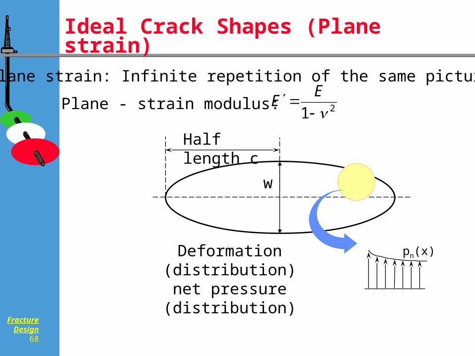
Ideal Crack Shapes (Plane strain)

Half length c

pn(x)

Deformation (distribution)net pressure (distribution)

21

EEPlane - strain modulus:

w

Plane strain: Infinite repetition of the same picture (2D)

FractureDesign

69

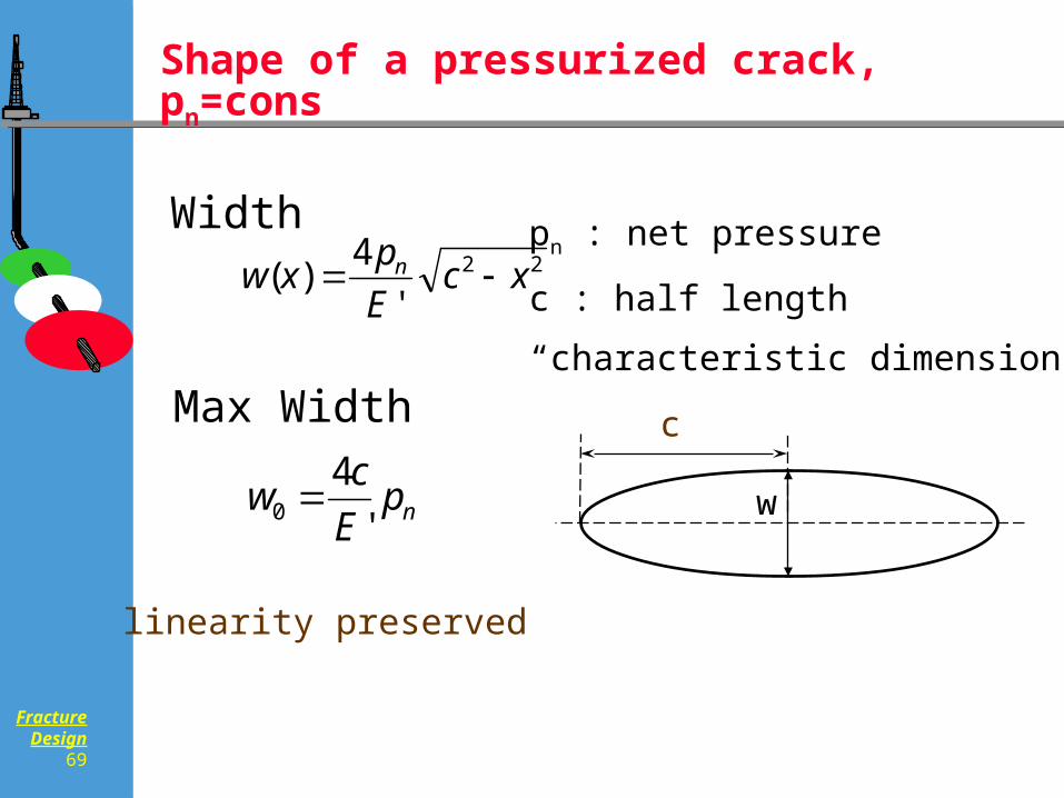
Shape of a pressurized crack, pn=cons

pn : net pressure

c : half length

“characteristic dimension”

22

'

4)( xc

E

pxw n

npE

cw

'

40

Width

Max Width

linearity preserved

w

c

FractureDesign

70

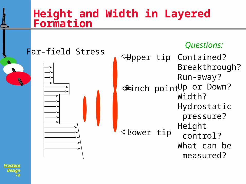
Height and Width in Layered Formation

Pinch point

Contained?Breakthrough?Run-away?Up or Down?Width?Hydrostatic pressure?Height control?What can be measured?

Upper tip Far-field Stress

Lower tip

Questions:

FractureDesign

71

From Fracture Mechanics to Fracture Height

FractureDesign

72

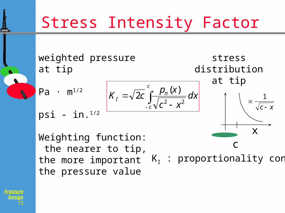
Stress Intensity Factor

weighted pressure at tip

Pa · m1/2

psi - in.1/2

Weighting function: the nearer to tip, the more important the pressure value

stress distributionat tip

c

c

nI dx

xc

xpcK

22

)(2

xc

KI : proportionality const

xc

1

FractureDesign

73

Stability of Crack, Propagation

Critical value of stress intensity factor:

Fracture Toughness KIC

Propagation: when stress intensity factor

is larger than fracture toughness

FractureDesign

74

Application: Fracture Height Prediction

Height containment: why is it critical?

Fracturing to water or gas

Wasting proppant and fluid

Can it be controlled?

Passive: safety limit on injection pressure

Active: proppant (light and heavy)

FractureDesign

75

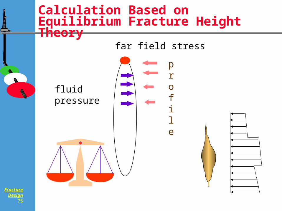
Calculation Based on Equilibrium Fracture Height Theory

fluid pressure

far field stress

profile

FractureDesign

76

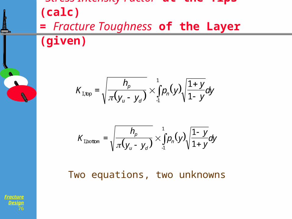
Stress Intensity Factor at the Tips (calc) = Fracture Toughness of the Layer (given)

Kh

y yp y

y

ydy

p

u dnI,top

-1

1

=

1

1

Kh

y yp y

y

ydy

p

u dnI,bottom

-1

1

=

1

1

Two equations, two unknowns

FractureDesign

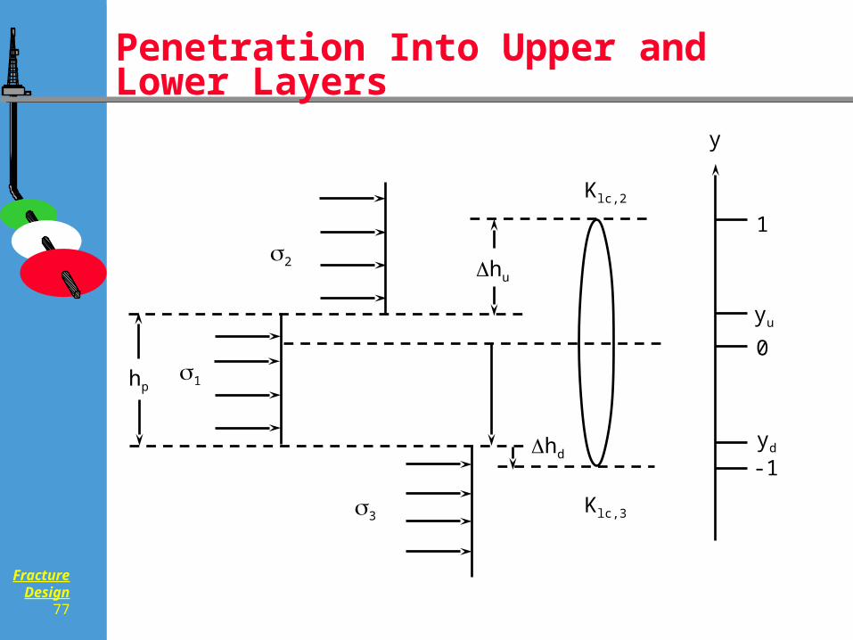
77

Penetration Into Upper and Lower Layers

hp

Klc,2

hu

y

0

3

1

2

Klc,3

hd

1

yu

yd

-1

FractureDesign

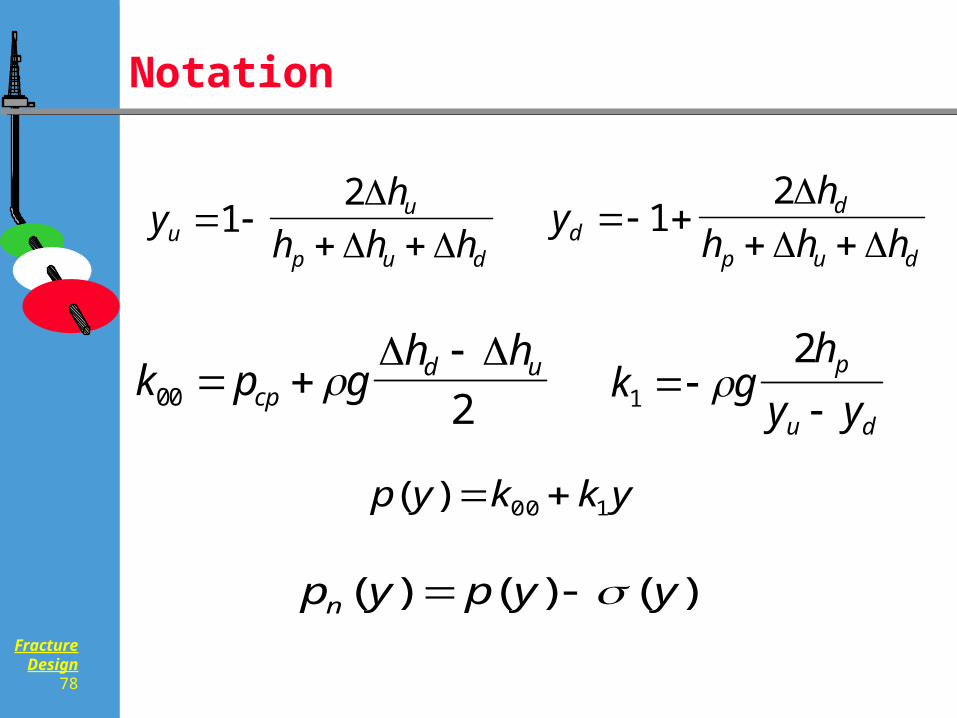
78

yh

h h huu

p u d

12

yh

h h hdd

p u d

12

k p gh h

cpd u

00 2

k gh

y yp

u d1

2

ykkyp 100)(

Notation

)()()( yypypn

FractureDesign

79

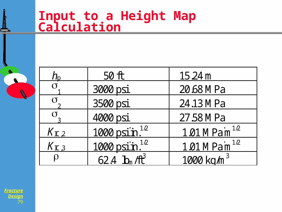
Input to a Height Map Calculation

hp 50 ft 15.24 m

1 3000 psi 20.68 MPa

2 3500 psi 24.13 MPa

3 4000 psi 27.58 MPaKIC,2 1000 psiin.1/2 1.01 MPam1/2

KIC,3 1000 psiin.1/2 1.01 MPam1/2

62.4 lbm/ft3 1000 kg/m3

FractureDesign

80

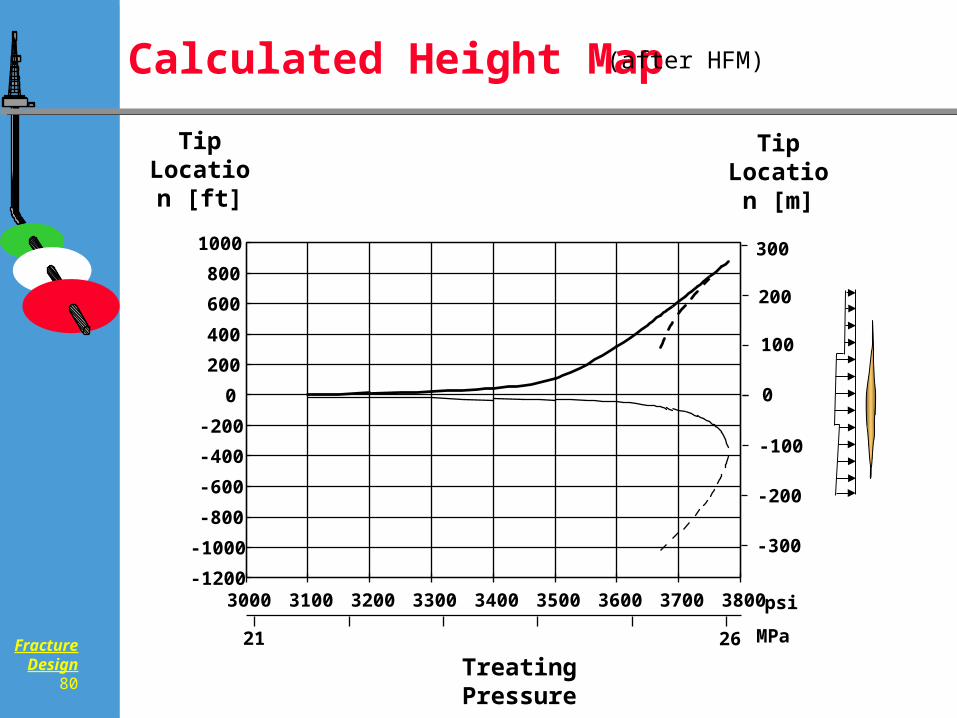
Calculated Height Map

-1200

-1000

-800

-600

-400

-200

0

200

400

600

800

1000

3000 3100 3200 3300 3400 3500 3600 3700 3800

300

-300

0

21 26

psi

MPa

200

100

-100

-200

Tip Location

[m]

Tip Location

[ft]

Treating Pressure

(after HFM)

FractureDesign

81

How to Use a Height Map?

1 Off-line:

Assume a height, make a 2D design,

Calculate net pressure (averaged in time)

Read-off a better estimate of height

2 In-line:

P3D design (3D),

Calculate net pressure at a location

Adjust height to equilibrium

FractureDesign

82

Fluid loss: the property of both the rock and the fluid

1 Leak-off2 Spurt loss

FractureDesign

83

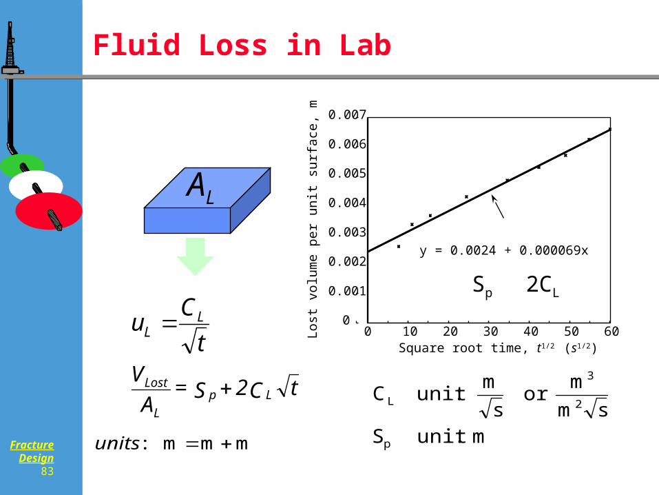
Fluid Loss in Lab

t

Cu L

L

tC2S=A

VLp

L

Lost

mmm : units

AL

m :unit Ssm

mor

s

m :unit C

p

2

3

L

y = 0.0024 + 0.000069x

0 10 20 30 40 50 60Square root time, t1/2 (s1/2)

0

0.001

0.002

0.003

0.004

0.005

0.006

0.007

Lost

vol

ume

per

unit

surf

ace,

m

2CLSp

FractureDesign

84

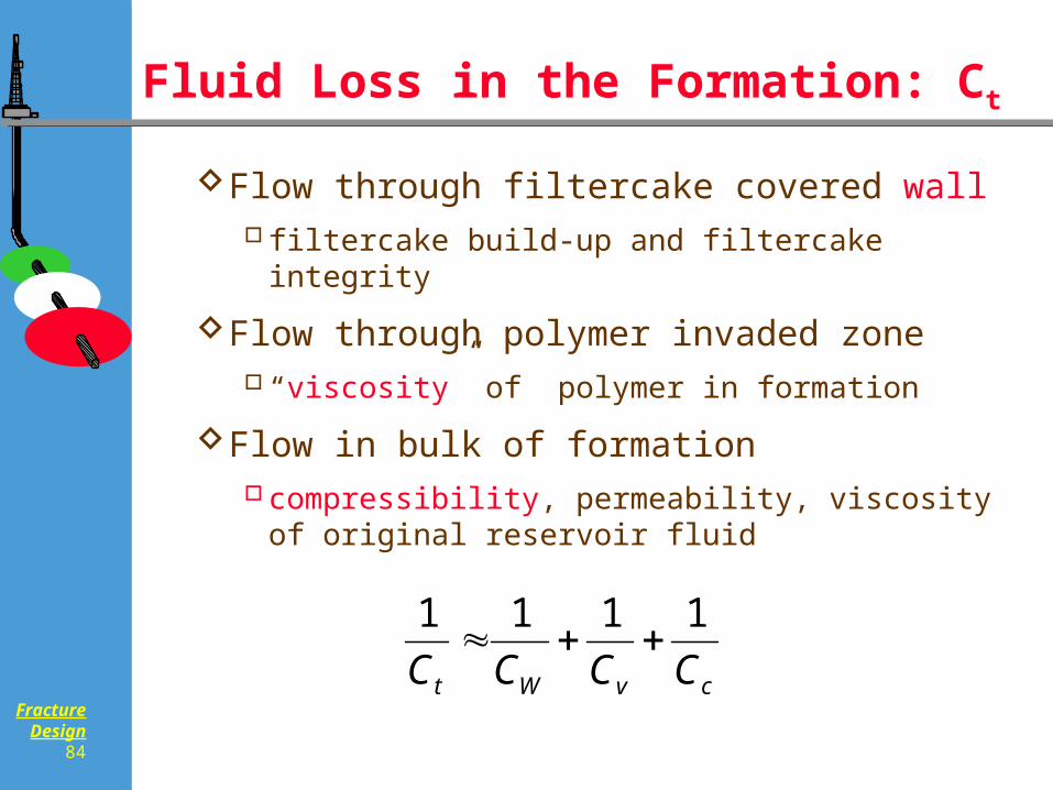
Fluid Loss in the Formation: Ct

Flow through filtercake covered wallfiltercake build-up and filtercake integrity

Flow through polymer invaded zone“viscosity” of polymer in formation

Flow in bulk of formationcompressibility, permeability, viscosity of

original reservoir fluid

cvWt CCCC

1111

FractureDesign

85

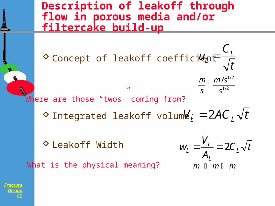
Description of leakoff through flow in porous media and/or filtercake build-up

Concept of leakoff coefficient

Integrated leakoff volume:

Leakoff Width

t

Cu L

L

tACV LL 2

tCA

Vw L

L

LL 2

2/1

2/1/

s

sm

s

m

mmm

Where are those “twos” coming from?

What is the physical meaning?

FractureDesign

86

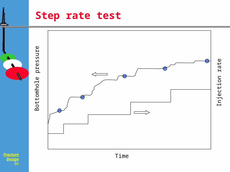
Step rate test

Time

Bot

tom

hole

pre

ssur

e

Inje

ctio

n ra

te

FractureDesign

87

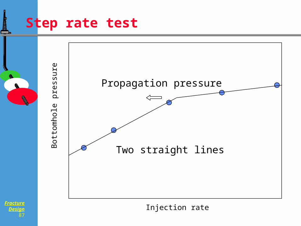
Step rate test

Injection rate

Bot

tom

hole

pre

ssur

e

Propagation pressure

Two straight lines

FractureDesign

88

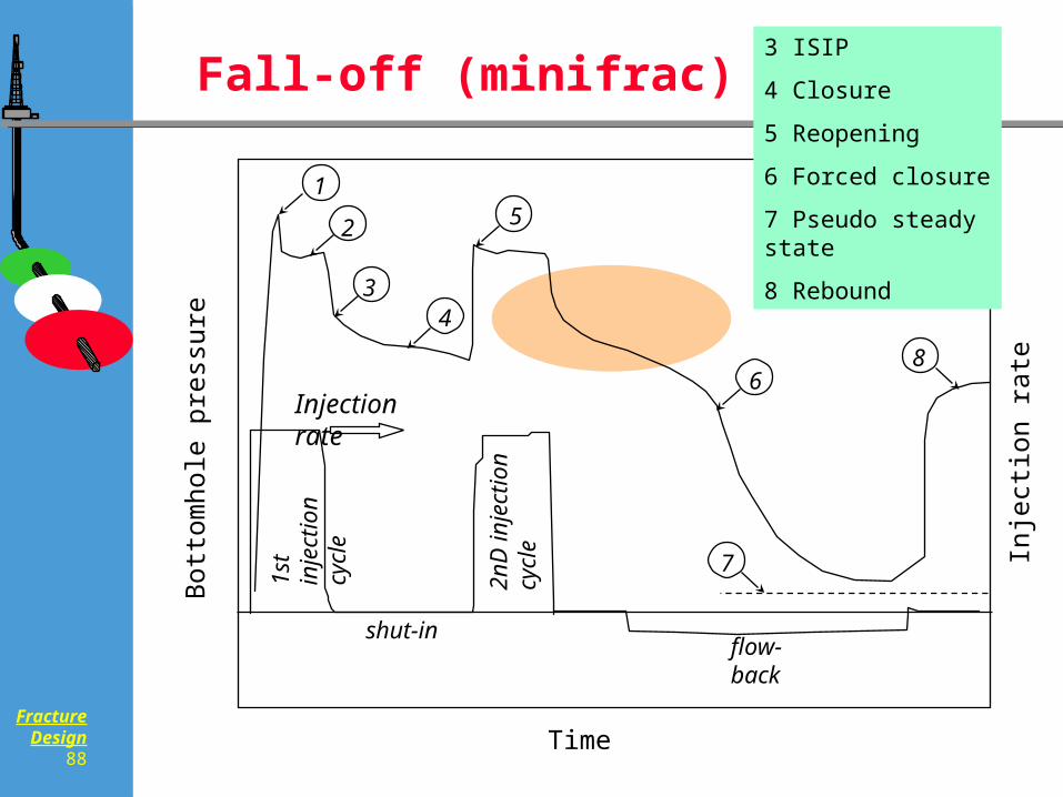
Fall-off (minifrac)

1st

inje

ctio

n cy

cle

2nD

inje

ctio

n cy

cle

flow-backshut-in

1

2

34

5

68

7

Injection rate

Time

Bot

tom

hole

pre

ssur

e

Inje

ctio

n ra

te

3 ISIP

4 Closure

5 Reopening

6 Forced closure

7 Pseudo steady state

8 Rebound

FractureDesign

89

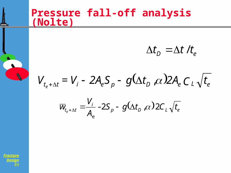
Pressure fall-off analysis(Nolte)

eLeDpeitt tC2AtgS2AV=Ve

,

eD ttt /

eLDpi

tt tCtgSA

Vw

e2 ,2-

e

FractureDesign

90

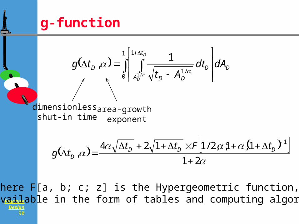
g-function

where F[a, b; c; z] is the Hypergeometric function, available in the form of tables and computing algorithms

dimensionless shut-in time

area-growth exponent

D

t

A

D

DD

D dAdtAt

tgD

D

1

0

1

/1/1

1,

21

1;1;,2/1124,

1

DDDD

tFtttg

FractureDesign

91

g-function

FractureDesign

92

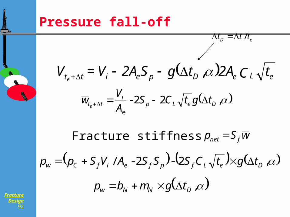
Pressure fall-off

,2-2-/ DeLfpfeifCw tgtCSSSAVSpp

p b m g tw N N D ,

eLeDpeitt tC2AtgS2AV=Ve

,

eD ttt /

,22- e

DeLpi

tt tgtCSA

Vw

e

wSp fnet Fracture stiffness

FractureDesign

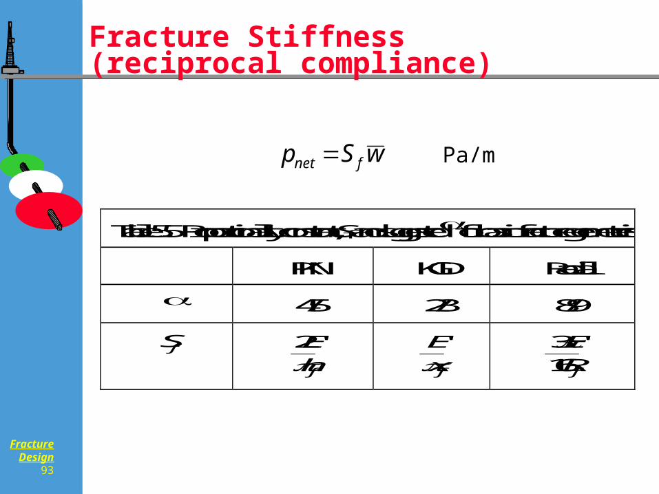
93

Fracture Stiffness(reciprocal compliance)

Table 5.5 Proportionality constant, Sf and suggested for basic fracture geometries

PKN KGD Radial

4/5 2/3 8/9

Sf 2E

hf

'

E

xf

'

3

16

ERf

'

wSp fnet Pa/m

FractureDesign

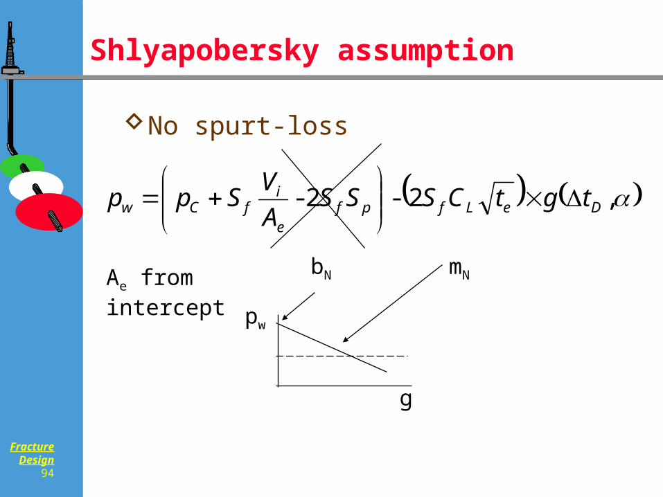
94

Shlyapobersky assumption

No spurt-loss

,2-2- DeLfpfe

ifCw tgtCSSS

A

VSpp

Ae from intercept

g

pw

bN mN

FractureDesign

95

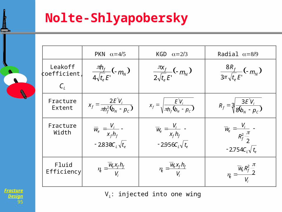
Nolte-Shlyapobersky

PKN KGD Radial

Leakoffcoefficient,

CL

N

e

f mEt

h

'4

N

e

f mEt

x

'2

N

e

f mEt

R

'3

8

FractureExtent CNf

if

pbh

VEx

2

2 CNf

if

pbh

VEx

3

8

3

CN

if

pb

VER

FractureWidth

eL

ff

ie

tC

hx

Vw

830.2

eL

ff

ie

tC

hx

Vw

956.2

eL

f

ie

tC

R

Vw

754.2

22

FluidEfficiency

i

ffee

V

hxw

i

ffee

V

hxw

i

fe

eV

Rw2

2

Vi: injected into one wing