Fracking Growth

Thiemo Fetzer ∗

March 28, 2014

Abstract

This paper estimates the effect of the shale oil and gas boom in the United Stateson local economic outcomes. The main source of exogenous variation to be ex-plored is the location of previously unexplored shale deposits. These have becometechnologically recoverable through the use of hydraulic fracturing and horizontaldrilling. I use this to estimate the localised effects from resource extraction. Everyoil- and gas sector job creates about 2.17 other jobs. Personal incomes increase by8% in counties with at least one unconventional oil or gas well. The resource boomtranslates into an overall increase in employment by between 500,000 - 600,000 jobs.A key observation is that, despite rising labour costs, there is no Dutch disease con-traction in the tradable goods sector, while the non-tradable goods sector contracts.I reconcile this finding by providing evidence that the resource boom may give riseto local comparative advantage, through locally lower energy cost. This allows aclean separation of the energy price effect distinct from the local resource extractioneffects.

Keywords: resource boom, fracking, shale, spillovers, natural gas, energy pricesJEL Codes: Q33, O13, N52, R11, L71

∗An earlier version dated October 13, 2013 had been circulating under the same title. LondonSchool of Economics and STICERD, Houghton Street, WCA2 2AE London. Support from the Kondard-Adenauer Foundation is gratefully acknowledged. For the most recent version of this paper, pleaserefer to http://www.trfetzer.com. I would like to thank Tim Besley, Jon de Quidt, Jon Colmer, MirkoDraca, Claudia Eger, Jakob Fetzer, Christian Fons-Rosen, Maitreesh Ghatak, Benjamin Guin, Sam Mar-den, Hannes Mueller, Gerard Padro-i-Miquel, Pedro Souza, Daniel Sturm, Kelly Zhang and seminarparticipants at LSE, CEP, Oxford University and IAE Barcelona for helpful comments. In addition, Iwould like to thank Simen Gaure for developing the lfe package for R and Tu Tran at the EIA for kindlysharing some data.

1

1 Introduction

The role of energy prices and its relationship with economic aggregates such asemployment, wages, and output has been a key concern for academic economistsince the oil price shocks in the 1970s (Berndt and Wood (1975)). A second literaturethat developed around the same time was studying the impact of resource boomson economic outcomes, originally at the aggregate level (Bruno and Sachs (1982),Corden and Neary (1982a)) and then increasingly through micro-econometric stud-ies (see Michaels (2011), Black et al. (2005)). The key empirical observation fromthis literature was that resources can be, both a blessing and a curse. This paperaims to link these two strands of literature. I exploit the recent energy boom in theUS as a window through which I can study both, the local effects of lower energyprices and the local effects of the extraction activity itself. I show that it may be thecombination of these two forces that can help explain why a resource boom may bea disease for some and a blessing for other countries.

The identification will rely on two sources of arguably exogenous variation.First, I exploit spatial variation in resource extraction of shale deposits that becamerecoverable due to technological advances in drilling technology. The second sourceof exogenous variation is driven by the implied changes in the energy productiongeography of the US; moving natural gas production from the South to the MidWest and the North East of the country does not have the existing pipeline capacityto take the produce to market where the willingness to pay is highest; this generatesdistinctly lower gas prices.

In the last step, I combine the findings from these empirical approaches andhighlight that they may help us understand why there is no resource curse in sec-tors that may be particularly vulnerable to it.

It is important to highlight the context in which this recent energy boom ishappening. Since the early 2000s, US domestic natural gas and oil production wasin decline and the imports of crude and natural gas became even more importantas they had already been. Employment in the natural gas and oil extraction sectorwas at its lowest since 1972.

In 2012, the picture is vastly different. The transition that was achieved in thelast 7 years falls short from being a miracle. The US, in 2012, is least dependenton foreign energy imports than it ever was since 1973. This is attributed to im-provements in energy efficiency and the development of biofuels. However, themost important contributing factor is the development of unconventional resourceextraction technology known as hydraulic fracturing or “fracking” that has lead toa mining boom across the US. The hydraulic fracturing technology, together withhorizontal drilling made vast shale deposits accessible, that could previously not

2

be economically exploited. As a consequence, employment in the mining sector hasreached levels not seen since the early 1990s. But do these employment gains havesignificant spill-over effects into different sectors at the locations where resourceextraction is actually taking place? It is - by no means - clear, whether one shouldexpect significant employment gains in the non-mining sectors. The developmentliterature has highlighted that it strongly depends, among others, on the type ofresources (Boschini (2007), Mehlum et al. (2006)), the quality of the institutions (Vi-cente (2010),Sala-i Martin and Subramanian (2003),Robinson et al. (2006),Monteiro(2009), Caselli and Michaels (2012), Ross (2006)), the potential for input demandlinkages (see Aragon and Rud (2013)) and the extent to which revenues are in-vested locally (Caselli and Michaels (2012)).

The first contribution of this paper is to quantify the extent of the local effectsdue to the recent resource boom. I show that many economic aggregates, such aslocal employment, payroll, labour force participation and unemployment respondquite significantly. In the next step I highlight that this is driving up local wagesacross the sectors, giving rise the the possibility of there being a resource curse. Inthe third step I find no evidence that the manufacturing sector suffers from Dutchdisease style contraction, while the non-tradable goods sector does.

In the last section I explore whether locally cheaper energy may explain thisfinding. Energy is a key factor of production for many production processes - bothdirectly and indirectly, through intermediate goods consumption. The literatureon electricity prices and provision has highlighted the relevance and importance ofcheap and in particular, reliable energy (see e.g. Rud (2012), Abeberese (2012) andFisher-Vanden et al. (2012)) or Dinkelman (2011), who studies the labour marketeffects of electrification in South Africa. In the case of the US, Kahn and Mansur(2013) show that electricity prices affect firm location decisions, while Severnini(2013)’s analysis suggests that low energy prices in the historical context may havecreated agglomeration clusters. I proceed to show that indeed - energy intensivetradable goods sectors - do expand, giving initial credence to this mechanism.

Following this I show that natural gas and electricity become significantly cheaperin counties with shale deposits from the mid 2000s onwards, suggesting that higherlabour costs may be offset with lower energy bills. I show that the effect is particu-larly pronounced in places that face significant pipeline capacity constraints. Bind-ing outflow capacity forces the additionally extracted natural gas to be consumedlocally, putting downward pressure on local prices.

In the last step I provide a small back of the envelope calculation that indicatesthat the drop in energy prices offsets the increase in labour costs, which may explainwhy the local non-tradable goods sector contracts, while the tradable goods sectordoesn’t. This highlights that a key to understanding whether Dutch disease style

3

contractions do occur, depends on the nature of the resource and whether thereare significant trade costs associated with the export of the latter. This ties in wellwith the arguments in Boschini (2007), who argue that the type of resource mattersfor whether a country actually suffers from a resource curse. They mainly arguethat this is driven by the degree to which the resource can be appropriated. Themechanism I explore here highlights that it depends on the extent of trade costsand frictions, as these create locally lower energy prices.

The paper is organised as follows. I begin with a very brief conceptual frame-work to guide the empirical analysis. In the third section I discuss the main datasources used. The fourth section then proceeds to establish the main results, whilethe fifth section focuses on the proposed mechanism of lower natural gas prices.The last section concludes.

2 Conceptual Framework

Before discussing the data used in this paper and the empirical specifications, Iwant to present a simple conceptual framework to fix some ideas and to motivatethe empirical analysis.

I build on the simple partial-equilibrium framework in Corden and Neary (1982b).I assume that there are three sectors: the resource or energy production sector, atradable goods sector and a non-tradable goods sector. These are indexed withE, T, NT and have production functions E = Ah(NE), YNT = Bg(NNT) and YT =

f (NT, E). This simple formulation implicitly assumes that the tradable goods sec-tor is relatively more energy intensive than the non-tradable goods sector. All threesectors compete for an immobile factor labour. The price of tradable goods servesas the numeraire. In the first exercise, I assume that energy prices and the priceof tradables is fixed and only wages and the price of non-tradables may respondto a productivity shock in the resource extraction sector. This mimics the case of asmall open economy and gives rise to the classical results as in Corden and Neary(1982b). In the second exercise, I model a wedge in local energy prices that is afunction of the bindingness of pipeline capacity constraints (e.g. a lack of takeawaycapacity). This generates a local market for energy and thus implies that there is afeedback from lower energy prices. Households have simple Cobb-Douglas utilityover consumption of tradables and non-tradables.

u(YT, YNT) = αT log(YT) + αNT log(YNT)

Income in this economy is simply y = w + θπE, where πE are the profits thataccrue in the energy production sector and θ is a measure indicating the extent

4

to which these profits go to local owners of the mineral resources. The demandfunctions for non-tradables is simply Yd

NT = αNTy

pNT. The market clearing condition

in the labour market requires:

NdNT + Nd

T + NdE = 1

.where the labour- and energy demand functions solve the following first order

conditions.

pE Ah′(NdE) = w

pNTBg′(NdNT) = w

Two for the tradable sector:

pT f1(NdT, Ed) = w

pT f2(NdT, Ed) = pE

For fixed energy prices, an increase in the productivity in the resource extrac-tion sector, has three effects. Firstly, the increase in productivity is going to lead toan overall increase in aggregate economic activity and GDP per capita. The secondand third effects are concerned about the effect on wages and the implied impacton the allocation of labour across sectors. First, there is the resource movement effect.As labour demand by the resource sector increases, overall wages go up. This im-plies that the marginal cost of production for non-tradables and tradables increase.Hence, the employment shares of these sectors contract. There is a direct factorprice induced structural transformation. Graphically this is indicated in Figure 1.

The second effect is the so-called spending effect. Higher equilibrium wages driveup local incomes y, which is inducing an outward shift in the demand for tradables-and non-tradables for a given level of prices. This increased demand leads to anincrease in production in the non-tradables sector, thus, partly offsetting the im-plied contraction due to the resource movement effect. Wages increase even furtherand thus, lead to a further contraction of the tradable good sector. The sum ofthe spending and resource movement effect suggests an unambiguous increase inwages and thus, a contraction in the tradable goods sector, but not necessarily inthe non-tradable goods sector due to the spending effect. The degree to which thespending effect may offset the resource movement effect depends on the elasticityof demand for non-tradables with respect to income.

Consider now the case of variable energy prices. In particular, I assume that en-

5

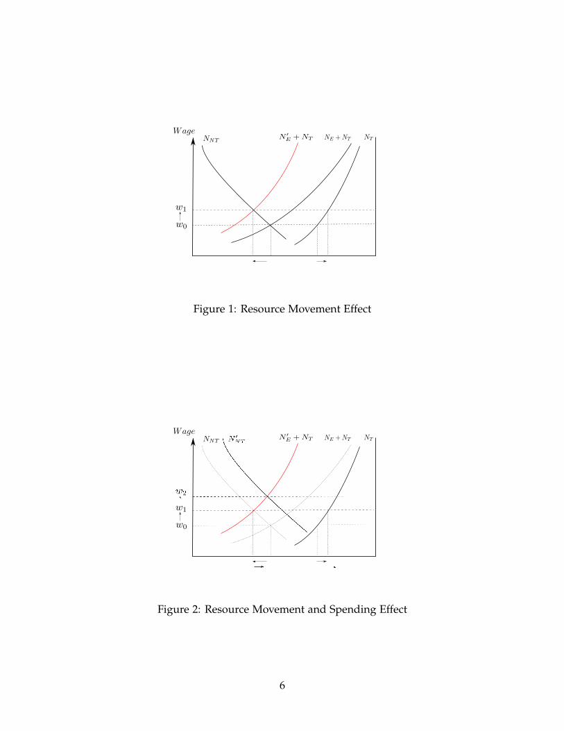
Figure 1: Resource Movement Effect

Figure 2: Resource Movement and Spending Effect

6

ergy prices pE are exogenously given, but local energy prices pE may be lower thanpE. Local energy price differentials reflect the extent to which energy is tradable.For energy, such as natural gas or electricity there are mechanic trade costs, as thetransport of the commodity uses up part of the commodity itself.1 I assume thatlocal energy prices are given as:

pE = τ(E) pE

with τ(E) < 1. The degree of the price wedge depends on a set of characteris-tics, such as pipeline transmission constraints and the physically implied transportcosts.

Given this reduced form representation of the local energy market, there is nowa distinct margin through which an increase in productivity in energy productionaffects the tradable goods sector. With endogenous local energy prices, the increasein the productivity of the energy production sector is correlated with lower localenergy prices, which may provide insurance against the increase in labour costs.A reduction in the energy prices does not have a direct effect on the non-tradablegoods sector, but it does have an impact on the energy and the tradable goodssector. First, it is going to moderate the initial movement of labour into the energysector as the marginal returns are now decreasing in the level of output and second,the lower energy price is going to increase the demand for labour by the tradablesector depending on the degree of complementarity. This further increases wages,while hurting the non-tradable goods sector, as the latter is not able to benefit fromlower energy prices; the key observation is that an energy price effect may nowgenerate ambiguous effects for all three sectors.

The degree of ambiguity depends on the relative strength of the resource-movementeffect compared to the spending effect and the energy price effect. The key vari-ables of interest here are the labour intensity relative to the labour intensity for theinterplay of the energy price effect and the spending effect and the income elastic-ity of demand for non-tradables, which measures the degree to which the spendingeffect affects the non-tradable goods sector.

The ambiguous predictions for the relative employment shares make this verymuch an empirical question. I will proceed in three steps that follow naturally fromthis analysis.

1For natural gas, 11% of the extracted natural gas is used in the transmission process by compressorstations along the natural gas pipeline grid. For electricity, aggregate transmission losses account for 7%of gross electricity generation.

7

3 Data

Shale Plays, Oil- and Gas Well Location Data

The key empirical design will be simple intention-to-treat exercises exploiting geo-graphic variation in the availability of unconventional oil and gas resources. Thisdata was obtained from the Energy Information Administration and the US Geo-logical Survey and is presented as the grey areas in Figure 3.

The second main source of data is a set of geocoded locations of actual uncon-ventional oil or gas wells where unconventional techniques involving horizontaldrilling and hydraulic fracturing are applied. This data was derived from variousstate-level sources and the data disclosure website Frac Focus. The data is discussedin further detail in Appendix A.1. Based on these data I construct a cross-sectionaldummy indicating the presence of an unconventional well in a county by 2012. Thisdummy variable provides cleaner treatment assignment and does not merely reflectthe intention to treat, since not all shale resources are currently being actively pur-sued. The resulting map of well locations is presented in Figure 3. The reason forusing the cross-section of well locations is one of data constraints; not for all wellsin the sample do I have data on the actual timing of when a well was constructed.The unconventional shale gas and oil boom commenced in 2005, however, the tim-ing varies across shale plays. I have the exact dates of when drilling operationscommenced for a set of states, appendix A.1 shows that new well construction issignificantly occurring from the mid 2000s onwards, which coincides well with theanecdotal accounts.

Sectoral Employment

They key outcome variables studied in this paper is annual sectoral employment, asobtained from the the Longitudinal Employer-Household Dynamics dataset main-tained by the US Census Bureau (see Davis et al. (2006) for a discussion). Thisdataset produces Quarterly Workforce Indicators (QWI) that provide details up to4-digit NAICS industry codes. The data covers 96% of all employment in the USand is developed to provide researchers with a very fine spatial- and temporal res-olution that can be further disaggregated by firm- characteristics, such as firm sizeand age or by individual employee characteristics such as age, educational attain-ment and race. The second key variable of interest is the earnings per worker data,which provides the average monthly earnings for a worker in a sector and countyin a given quarter, provided that this worker has been with the firm for the durationof the whole quarter. This variable will be used as a proxy for wages. Since estimat-ing high dimensional fixed effects can be computationally very heavy, I reduce the

8

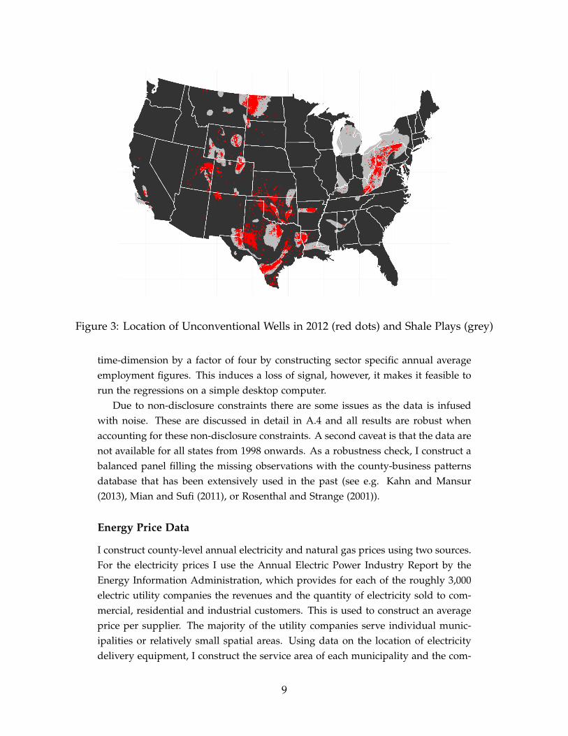
Figure 3: Location of Unconventional Wells in 2012 (red dots) and Shale Plays (grey)

time-dimension by a factor of four by constructing sector specific annual averageemployment figures. This induces a loss of signal, however, it makes it feasible torun the regressions on a simple desktop computer.

Due to non-disclosure constraints there are some issues as the data is infusedwith noise. These are discussed in detail in A.4 and all results are robust whenaccounting for these non-disclosure constraints. A second caveat is that the data arenot available for all states from 1998 onwards. As a robustness check, I construct abalanced panel filling the missing observations with the county-business patternsdatabase that has been extensively used in the past (see e.g. Kahn and Mansur(2013), Mian and Sufi (2011), or Rosenthal and Strange (2001)).

Energy Price Data

I construct county-level annual electricity and natural gas prices using two sources.For the electricity prices I use the Annual Electric Power Industry Report by theEnergy Information Administration, which provides for each of the roughly 3,000electric utility companies the revenues and the quantity of electricity sold to com-mercial, residential and industrial customers. This is used to construct an averageprice per supplier. The majority of the utility companies serve individual munic-ipalities or relatively small spatial areas. Using data on the location of electricitydelivery equipment, I construct the service area of each municipality and the com-

9

pute the average price charged.I proceed similarly for the natural gas prices using data collected by the En-

ergy Information Administration under Form EIA-176. This provides revenues andquantities of gas sold in a state and year for a local distribution company. Theservice areas were constructed based on confidential data from the EIA; it is onlyavailable for the year 2008, implying that changes in the service areas are not re-flected in my data. The average price of gas in a county is proxied by the simpleaverages of the prices charged by local distribution companies that service cus-tomers in a county. More details on the construction of these data are detailed inappendix A.3.

Pipeline Capacity Constraints

The Energy Information Administration provides data on state-to-state physicalpipeline capacity at an annual level as well as annual state-to-state pipeline flows.Figure A4 plots the resulting net physical capacity flows. For each state the annualdata provides information how much natural gas is flowing to all its neighbouringstates. Based on this, I can compute a state level measure of the bindingness of theexisting physical outflow- and inflow capacity. Let P be the set of states that areneighbouring state s, and Cps be the direct physical pipeline capacity connectingstate p ∈ P with state s, while Fps is the actually observed flow.

I simply compute

Os =∑p∈P Fps

∑p∈P Cps

as a measure of the bindingness of outflow capacity. Similarly, I compute Is

as a measure of the bindingness of inflow capacity. It is well-established that akey ingredient driving local natural gas prices is the bindingness of pipeline ca-pacity constraints; for electricity markets, this is very similar and has recently beenanalysed by Ryan (2013) in the Indian context.2

I construct the measure using the average capacity for the period 2000-2005 andthe average flows for that period. Averaging helps remove year-on-year variatione.g. induced by weather phenomena or other shocks, such as hurricanes, which mayadversely affect production in the outer continental shelf in the Gulf of Mexico.

The key intuition behind the various measures is that relatively binding outflowcapacity leads to locally lower natural gas prices, as additional local productionneeds to be locally consumed. This variation will be exploited to identify the effect

2On the natural gas spot market, the role of transmission constraints were very visible in recentmonths due to the strong winter driving up energy demand. Natural gas prices on the AlgonquinCitygate, near Boston, peaked at $ 95.00, averaging at $ 11 per cubic foot; prices in Louisiana peakedonly at $ 9.00 and averaged at $ 4.55 per cubic foot.

10

of the shale boom on local energy prices.I now proceed to present the main estimating equation along with the key re-

sults in turn.

4 Empirical Strategy and Results

This section presents the main estimation strategy along with the key results. Iuse two main specifications throughout the paper. The first one is to illustrate theoverall effect of the recent shale-gas and oil boom. For this, I consider the left-handside variables in levels as the conceptual framework indicates an overall economicexpansion due to the technological progress in the resource extraction sector. Forthese exercises I use a simple instrumental variables exercise using the presenceof shale-resources (the intention to treat) as an instrument for the cross section ofunconventional wells that were present by the end of 2012.

ycist = αci + bst + ∑i

γi × Shalec + X′β + νcist (1)

where αci is a set of county industry fixed effects, bst is a set of state-time fixedeffects, X is a set of other controls3 and Shalec measures the share of the land areain a county that is covered by unconventional shale resources. Standard errors willbe clustered at the state-level unless otherwise stated.

The main instrumental variables specification is

ycist = αci + bst + ∑t

ηt ×Yeart × Anywellc + X′β + εcist (2)

where Anywellc is a dummy variable that is equal to 1 in case there is an uncon-ventional well located in a county by 2012. These are instrumented with the set ofinteractions Yeart× Shalec. These specifications will allow the visual presentation ofmost regression results, however, I also report less demanding specifications whereI split the data into a pre- and post period with 2008 being the cutoff year.

The second set of exercises aims to highlight the impact of the expansion ofthe mining sector and how this affects the labour allocation across sectors. Forthis exercise, I instrument the share of mining sector employment with a post 2008variable interacted with the share of a county’s surface that has shale resources.That is the specification becomes:

3I construct a set of heating- and cooling degree days controls using the daily minimum- and maxi-mum temperature data based on the PRISM dataset, which comes at a spatial resolution of roughly 4 x4 kilometres. See appendix A.6 for more details.

11

ycist = αci + bst + η MiningSectorShare + X′β + εcist (3)

where the first stage is

MiningSectorSharecst = αc + bst + γ× Post2008× Shalec + X′β + νcist (4)

As the prediction of the conceptual framework for the labour market was aboutthe relative sector sizes, this design mimics the conceptual framework closely.

The empirical analysis will proceed in three steps. First, I show that there isindeed a significant expansion of oil- and gas employment in areas with shale re-sources, and an overall economic expansion in other economic aggregates such aslocal area income, and employment. Most of the effect is driven by increased labourforce participation and less unemployment, while I do not observe significant gainsin population. I will use the boom in the mining sector to measure the extent ofspill-overs. This is a margin that is not incorporated by the simple model, which,however, moderates any Dutch disease style contraction in the non- mining sec-tors. I then show that the mining sector expansion is correlated with significantlyhigher monthly earnings across most sectors; this is the only unambiguous predic-tion from the conceptual framework, however, there is some heterogeneity due tothe different skill requirements across sectors. In the third step, I present resultson the employment shares, which highlights that the simple logic of the resource-movement and spending effect do not provide the expected results. I then try toreconcile these findings by providing evidence of distinctly lower energy pricesfacing the tradable goods sector. A small back-of-the envelope calculation suggeststhat indeed - lower energy costs may explain why there is no contraction in thetradable goods sector relative to the non-tradable goods sectors.

Step 1: Shale Resources and Economic Expansion

I first present evidence on the impact of shale resources on overall economic expan-sion. I document this in three individual steps. First, I show that there is a dramaticexpansion in oil- and gas sector that sets on from about 2005 onwards.

In the next step, I study overall local labour market outcomes. I document dra-matic increases in overall employment, labour force participation and a significantreduction in unemployment rate. I show that this expansion extends beyond themining sector, indicating that there are significant spill-overs. I use this to estimatea job-creation elasticity, indicating the number of jobs that are created for each oil-and gas sector job.

The third part documents the impact on local area income and payroll; this

12

0.0

0.5

1.0

1.5

2001 2004 2007 2010Year

Est

imat

ed E

ffect

Employment (IV) Employment (Reduced Form) P-Value 0.10 0.05 0.01

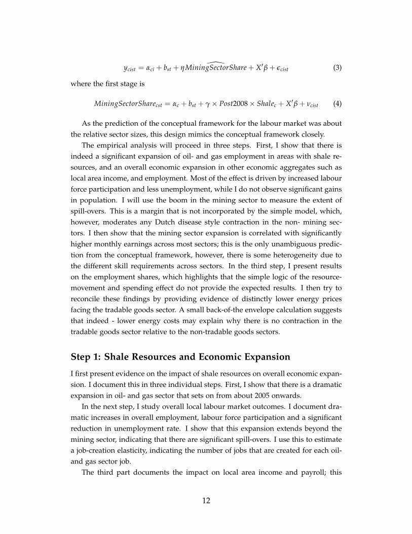
Figure 4: Expansion of Oil- and Gas Extraction Sector Employment

highlights that there is an overall increase in economic activity.The results from estimating models 1 and 2 are best presented graphically by

plotting the estimated coefficients ηt and γt, all accompanying tables can be foundin the online appendix.

Oil and Gas Sector Expansion Figure 4 presents the results from estimatingmodels 1 and 2, where I use the log of employment in the mining sector as thedependent variable. The pattern is very similar when using the share of oil- andgas sector employment as the dependent variable.

The coefficient plots are slightly unconventional. The line presents the estimatedcoefficients in the different years for the IV specification in red and the intention-to-tread reduced form in blue. The shade around the line becomes less opaque asthe estimated coefficients approach p-values near conventional significance levels.This highlights that the estimated effects are insignificant before 2006, which coin-cides well with the general accounts that fracking has only become a widespreadtechnology used from the mid 2000s onwards.

The estimated effects indicate how dramatic the expansion has been. The IVcoefficient suggests that places with unconventional oil or gas extraction activity

13

have experienced a growth in mining sector employment by 1.38 log points in 2012relative to control counties.4 The intention-to-treat estimates are, as expected, sig-nificantly lower suggesting an increase by 0.4 log points or 49% in 2012. Table 1presents the results from pooling into a pre- and post 2008 period. This year waschosen as the dynamics in most of these controls appear to be picking up fromthis point onwards. The results do not change significantly, if I use a differentbreak year. Clearly, there are some concerns about the onset of the financial crisiswith Lehman brothers collapse in late 2008. This will be addressed in detail invarious robustness checks. Column (1) presents the results for the mining sector,giving very similar results, suggesting an increase in mining sector employment byaround 1 log points.

Overall Local Economic Activity In the simple conceptual framework, theonly source for change in overall levels of local income is due to the technologi-cal progress in the oil- and gas sector. Hence, the increase in employment in theoil- and gas sector is not sufficient to highlight that there is indeed a local economicexpansion that can be ascribed to the boom in the oil and gas sector.

I now document that many economic aggregates respond to the boom in themining sector, indicating that there is indeed an increase in overall economic ac-tivity. The key variables I consider are measures of labour market activity, suchas unemployment, overall employment, non-mining sector employment, local areaincome and local area overall payroll.5

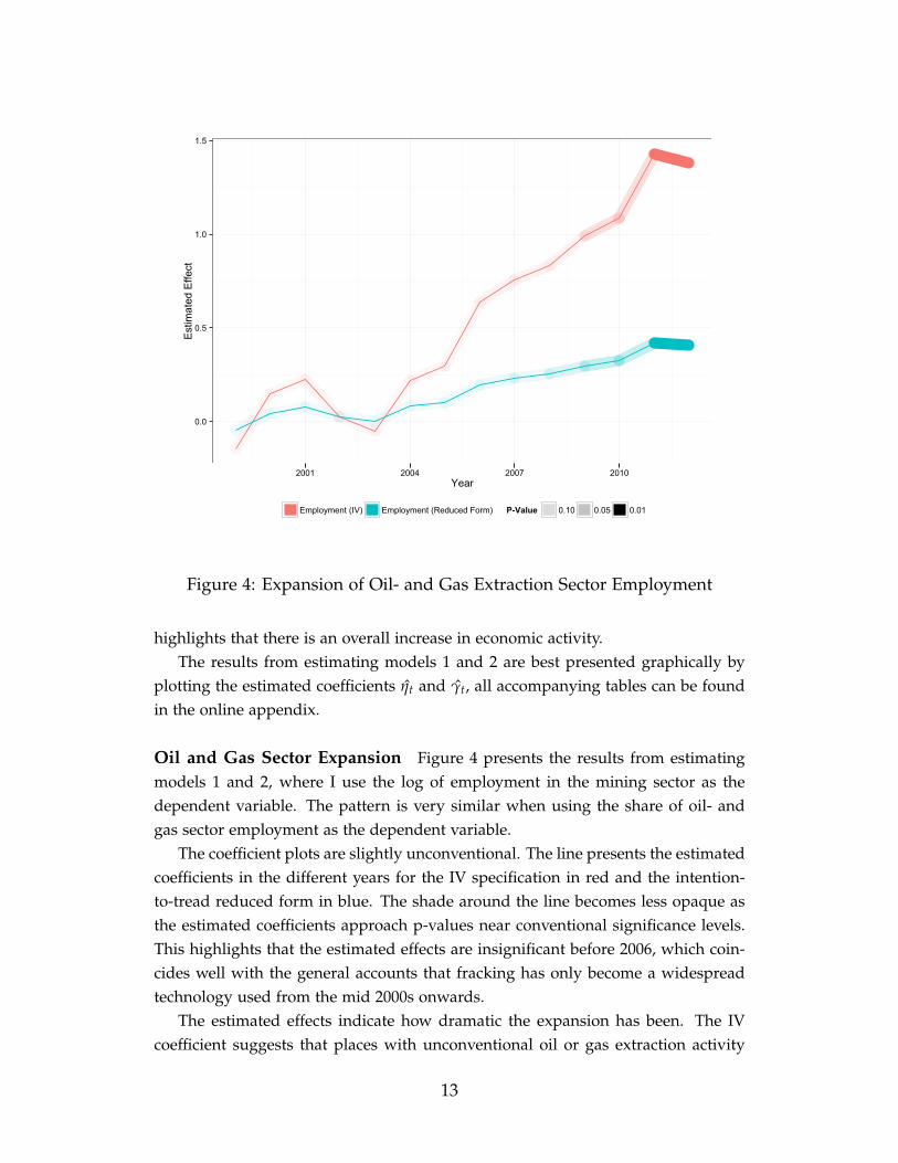
Figure 5 presents the core results for a set of economic indicators. The top panelpresents the IV results, while the bottom panel draws the estimated coefficients forthe intention to treat exercises. The opacity of the line is proportional to the p-valueof the estimated regression coefficient. The pattern that emerges is consistent.

Columns (2)-(7) of table 1 presents a regression version of the graphs. The re-sults indicate a significant expansion in non-mining sector expansion (see column3). This expansion is coming from increased labour force participation and signifi-cantly lower unemployment, as is indicated in columns (4) and (5). The coefficientsuggests that overall unemployment on counties with unconventional oil and gasis about 1.1 percentage points lower than for control counties.

Columns (6) and (7) explore the effects on local incomes. Personal incomes

4Note that the big increases can not simply be converted to proportional increases due to Jensen’sinequality, see Kennedy (1981). Thats why I leave them as log-points. For small values, the linearapproximation is reported.

5The local unemployment data is drawn from the Bureau of Labor Statistics Local Area Unemploy-ment Rate database, while the local area income data comes from the Bureau of Economic AnalysisRegional Economic Accounts. The remaining data is from the Quarterly Workforce Indicators describedin the data section.

14

0.05

0.10

0.15

0.20

2001 2004 2007 2010Year

Est

imat

ed E

ffect

Non Mining Overall P-Value 0.10 0.05

Employment

0.0

0.1

0.2

0.3

2001 2004 2007 2010Year

Est

imat

ed E

ffect

Payroll Personal Income P-Value 0.10 0.05 0.01

Income

0.00

0.05

0.10

0.15

2001 2004 2007 2010Year

Est

imat

ed E

ffect

P-Value 0.10 0.05 Labour Force Unemployment

Broader Labour Market

0.02

0.04

0.06

2001 2004 2007 2010Year

Est

imat

ed E

ffect

Non Mining Overall P-Value 0.10 0.05

Employment

0.00

0.03

0.06

0.09

2001 2004 2007 2010Year

Est

imat

ed E

ffect

Payroll Personal Income P-Value 0.10 0.05 0.01

Income

0.00

0.01

0.02

0.03

0.04

2001 2004 2007 2010Year

Est

imat

ed E

ffect

P-Value 0.10 0.05 Labour Force Unemployment

Broader Labour Market

Figure 5: Overall Effects on Employment, Non-Mining Employment and Local IncomeVariables

increase by around 8%, while the payroll increases by roughly 20%. This alreadyindicates that wage levels must be rising, as the overall employment increase incolumn (2) is just 10%, suggesting that wages must have gone up at least to someextent to bridge the difference.6

I now turn to exploring the extent to which the expansion in the oil and gas sec-tor creates spill-over job growth and the extent thereof. This is a particular mech-anism not incorporated in the simple conceptual framework, which may moderateany Dutch disease style contraction for local non-tradable goods producers.

Spill-Overs and Local Job Creation The expansion in the mining sector can beused as an instrument to estimate local multipliers for job creation, as e.g. exploredin Moretti (2010). This is important in this context as positive spill-overs indicatethat local non-tradable goods sectors, who benefit from such spill-overs due todemand linkages, may not actually contract in response of an expansion of the oiland gas sector, as they are benefiting directly through increased demand on topof the spending effect. In order to evaluate this, I use as instrument for oil andgas sector employment an interaction term Post2008× Shalec. This gives rise to theestimates in column (2) of table 2.

6An alternative explanation is increased working hours driving up overall payroll; this is a mechanismthat is, unfortunately, unobservable.

15

In the third column I use the estimated elasticity from column (2) and multiplythis by the means of the respective employment variables.7

I study four sectors separately. The first is the overall-non mining sector em-ployment. This suggests that for every oil and gas sector job, on average, 2.17non-mining sector jobs are created. The effect is mainly driven by growth inconstruction- and transportation sectors, which are strongly linked with the oil andgas industry. The other main employment categories do not experience statisticallysignificant spill-overs. Given that overall employment in the oil and gas sector hasmore than doubled between 2004 and 2013, increasing by 264,900 from 316,700 to581,500 this translates into an increase in overall employment by around 574,833due to the shale oil and gas boom. This represents a significant share of roughly0.4% of all employment in the US in 2012.

Step 2: Response of Wages and Earnings

The preceding results already indicate that there must be an increase of local wagesin response to the resource boom, since the overall payroll increases more than theoverall employment as indicated in 5. I now document the effect on real wages,highlighting that the estimated effect is a real wage increase, rather than a nominalone, as predicted by the simple framework. 8

I estimate specification 3, predicting the share of mining sector employmentwith the interaction term Post2008× Shalec as before.

The results are presented in table 3. Column (1) suggests that an increase inthe mining sector share by one percentage point increases monthly earnings in thatsector by 6 percentage points. Columns (2) - (6) provide the respective effects forthe different sectors. Column (3) and (4) present the results for the construction andtransportation sector wages. These are directly linked to the mining sector throughmining sector demand.9 The local manufacturing and service sector wages respondin similar fashion: a 1 percentage point increase in the mining employment share

7I only include observations up to the 95% percentile of the total non-mining sector employment. Thisbecomes necessary as the employment and population data is highly skewed, distorting the means whenincluding the upper quantiles. In the regressions, the skewness is taken care of by using logarithmictransformation, making conditional mean regressions appropriate.

8I construct local price-indices by combining a series of Consumer Price Indices for metropolitan sta-tistical areas, Census regions and Census region by city size drawn from the Bureau of Labour Statistics.I assign the CPI level to a county provided it falls in one of the metropolitan statistical areas that haveits own dedicated CPI series. For the remaining ones, I compute the weighted average of the CPI usingthe Census region and city size CPI series using as weights the population of a county that falls in eachtown-size class for which a separate CPI value for that respective region is available.

9The New York Department of Energy Conservation estimates that the construction of each wellrequires between 895 to 1350 truck loads, see http://www.dec.ny.gov/energy/58440.html, accessed on15.08.2013.

16

increases their respective wages by about 1.8 and 1.9 percentage points respectively.Since the mining sector share increased by around 3 percentage points on av-

erage, suggests that real wage costs for manufacturing firms increased by roughly5 percentage points. These results suggest that there is some heterogeneity in theextent of the wage increase. The effect is weaker for sectors with less of a factordemand linkage. However, overall, wages do increase significantly, which mirrorsthe findings of Allcott and Keniston (2013), who study the effects of oil and gasbooms on the manufacturing sector over the last thirty years. In the appendix, Ta-ble A4 presents the reduced form results by education group, confirming that thestrongest dynamics are observed for relatively low educational attainment levels.

The observed increase in real wages sets up the possibility for there to be aDutch disease style contraction in the tradable and non-tradable local sectors. Inthe next step I provide results that highlight that reallocation of labour across sec-tors in the manner suggested by the simple conceptual framework does not occur.The manufacturing sector does neither contract nor expand, while the non-tradableservice goods sector contracts.

Step 3: Employment Shares and Labour Reallocation

The conceptual framework without endogenous local energy prices, suggest thatthere be an unambiguously negative effect on the tradable goods sector, while theresponse of the relative size of the non-tradable goods sector is ambiguous. Thelatter depends on the strength of the spending effect.

I now explore the evolution of the sectoral shares over time. The results arepresented in table 4. The first column presents the result from specifications 2. Thisgives a sense of the overall impact of well-construction on shale deposits on theshare of mining sector employment; overall, mining sector employment increasedby around 3 percentage points, more than doubling the initial mining sector em-ployment share of roughly 2%. Columns (2)-(6) use the share of mining sectoremployment as a right hand side, instrumented for by the interaction Post 2008 xShale as in specification 3.

Column (2) indicates that the manufacturing sector appears not to be contract-ing. The coefficient on the share of manufacturing employment is negative but farform being statistically significant. Column (3) suggests that a one percentage pointincrease in mining sector employment increases the construction employment shareby 0.453 percentage points. The stark observation is that for locally consumed ser-vices (column (5) and (6)), the coefficient is unambiguously negative. This suggeststhat the reallocation of labour across sectors happens at the expense of the localnon-tradable goods sector, rather than at the expense of the tradable goods sector.

17

This is quite at odds with the conceptual framework, which suggested that the localnon-tradable goods sector might even expand if the spending effect is sufficientlystrong. The results presented here suggest that this is not the case, i.e. the spendingeffect appears to be quite week.

The next section highlights that the local tradable goods sector may even ex-pand, despite rising labour cost. I argue that this is driven by the fact that localenergy prices drop dramatically in response of the oil and gas boom. As tradablegoods sectors are more energy intensive, this offsets the increase in labour costs.This ties in well with the arguments in Boschini (2007), which argue that the typeof resource matters for whether a country actually suffers from a resource curse.They mainly argue that this is driven by the degree to which the resource can be ap-propriated. The mechanism I explore here highlights that it depends on the extentof trade costs and frictions.

5 Local Energy Prices and Sectoral Change

In this section I focus on one key mechanism that may explain why tradable goodssectors do not appear to contract, while other non-tradable goods sector appear tosuffer from a Dutch disease style contraction. I first present evidence that supportsthis mechanism: local sectors that are energy intensive do not contract. This holdsup when controlling for the extent to which the sectors are linked to the resourceextraction sector producing inputs for the latter, and a wide array of other controlvariables at the three digit industry level.

I then document that local energy prices do indeed contract significantly. Placeswith unconventional oil- and gas extraction experience drops in the costs of nat-ural gas by almost 30%. Similarly, local electricity prices go down significantly. Idocument that these effects are particularly pronounced in locations that are exportconstraint by the existing natural gas pipeline network, suggesting that trade costscan indeed be made responsible for these lower factor prices.

This suggests that in the short run, the boom in the resource extraction sectormay not necessarily crowd out local tradable goods producers. It may even attractfurther producers of energy intensive goods. There are anecdotal accounts suggest-ing that this is happening in the heart of America, with fertiliser producers buildingup capacity in the West of the US, taking advantage of lower energy prices there.10

In order to compare the degree to which different sectors vary in their use ofenergy as a source of input, I refer to the 2002 input-output tables developed by theBureau of Economic Analysis. Based on these, I construct measures of natural-gas

10See e.g. http://www.agweek.com/event/article/id/21548/publisher_ID/80/ for recent fertiliserplant construction in North Dakota.

18

intensity and overall utility intensity at the three digit industry sector level, as thereis significant variation within two digit industry.11

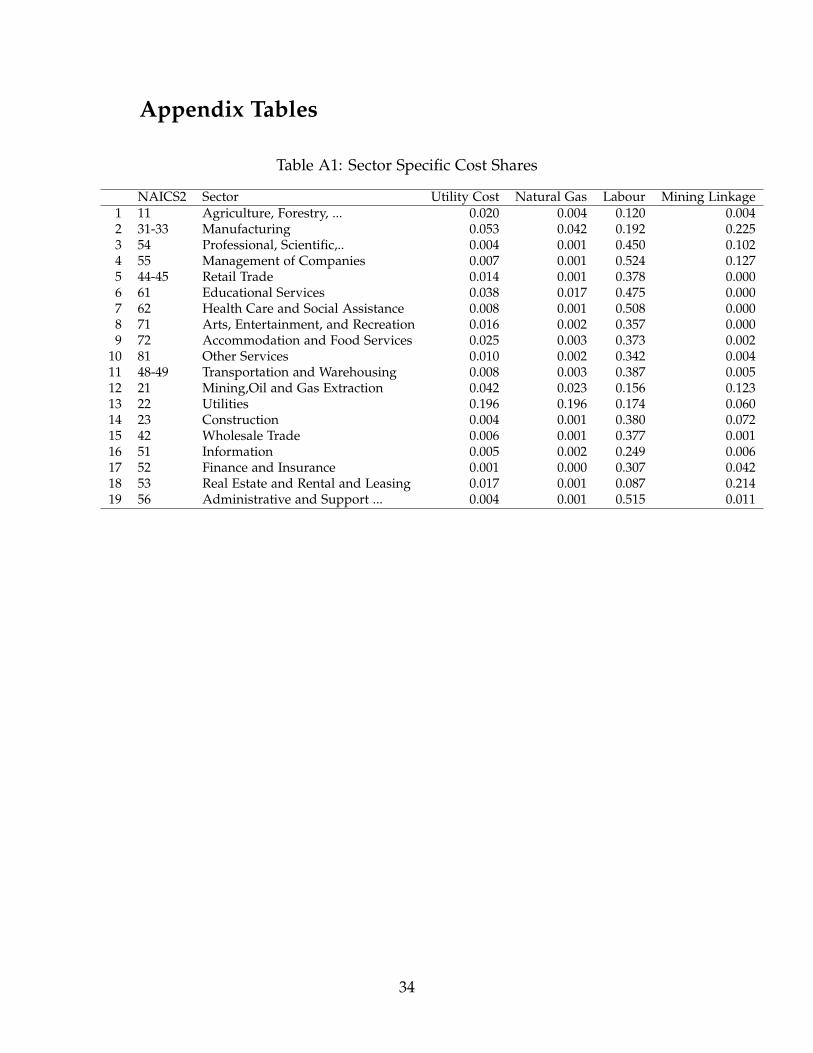
Using the same data-source, I also compute the labour cost shares as well as thedegree to which each sector is linked to the mining sectors by providing inputs forthe latter. This is an important control variable as it has been identified earlier thatthere are significant spillovers in the non-mining transportation- and constructionsectors, which may moderate any labour cost induced contraction. In the appendix,Table A1 provides these respective cost shares at the two-digit industry level.

All intensity measures are at the three digit level. Unfortunately, the input-output tables do not have the same sectoral break-up as the employment data. Inparticular, the retail- and wholesale trade sectors are all pooled together at the twodigit industry level. Thats why I focus the main results on just the manufacturingsector as there I have significant variation in energy intensity. I then successivelyadd more sectors in the control group to highlight that the estimated coefficientand patterns stay virtually the same and the results become even stronger.

Energy Intensity and Sector Specific Expansion In order to capture the sec-tor specific variation in energy intensity, I modify the estimating equation 1 byadding interaction terms with the sector specific energy intensity. The estimatingequation then becomes:

ycist = αci + bst + κ × Post2008× Shalec × EnergyIntensityi

+ γ× Post2008× EnergyIntensityi + X′β + νcist

where as left-hand side I use the log of sector specific employment. In order tocapture heterogeneity by different factor input intensities, I add further interactions.The results can be found in table 5.12

The first four columns constrain the analysis to only include the tradable goods

11In order to measure this, I compute the cost shares of natural gas in the input costs. For natural gas,I sum up all the purchased values from companies working in the Natural Gas Distribution, Oil- andGas Extraction 21100 and the Natural Gas Pipeline Transportation sectors (NAICS Codes 221200, 21100,486000 respectively). This gets as close as possible to the input cost shares of natural gas. For the broaderutility cost shares, I include all the above sectors and all electric utilities, that is private Electric PowerGeneration, Transmission and Distribution and State and local government electric utilities (NAICSCodes 2211000 and S00101, S00202).

I construct both measures of direct utility consumption as well as indirect utility consumption, indi-rectly used through the consumption of intermediary inputs.

12Note that the standard errors are clustered at the Workforce Investment Board Area level (WIA).This are regional entities created to implement the Workforce Investment Act of 1998. There are about7-8 counties per workforce investment board area, rendering them spatially still significant in size toaccount for spatial correlation. An appealing feature of the WIA is that they are designed to includecounties with similar economic structure, to ensure that the services under the Workforce InvestmentAct can be direct to the local needs.

19

industries.13 While the coefficient on the simple interaction of the time dummywith the shale deposit indicator is negative but insignificant, the coefficient on theenergy intensity interaction is positive and statistically significantly different fromzero. This coefficient does not change when adding more interactions as controlvariables, such as the downstream linkages or the labour cost share. Columns (5) -(7) include subsequently more sectors. In column (5) I add the non-tradable goodssector as control. As expected, the results get stronger.

This suggests that energy intensive tradable goods sector are actually benefitingfrom being on the shale. In the next section I highlight that this may be due to sig-nificantly lower energy prices, which allows tradable goods producers to competedespite rising labour costs.

Trade Costs and Local Energy Prices I show that local energy prices actuallygo down significantly. This reduction in energy prices is particularly observed forstates with shale deposits but that have relatively little slack natural gas pipelineoutflow capacity.

I estimate specifications 1 and 2 as before, however, now using local utility andelectricity prices as left-hand side variables.

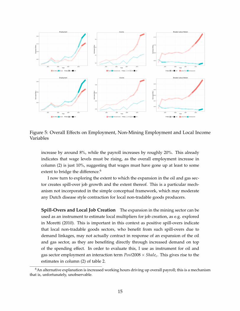
Figure 6 displays the estimated coefficients for local natural gas prices. It ap-pears that well before 2008 - if anything - natural gas prices in counties with shaledeposits had actually been higher than in the rest of the US. From 2008 onwards,this picture changes. By 2012, natural gas on places with shale deposits and activeresource extraction, was - on average - almost 30 percent cheaper than in the rest ofthe US.

Table 5 presents the reduced form results when exploring this relationship in amore systematic manner. In column (1) I present the reduced form effect of beingon the shale on natural gas prices by all uses. This suggests that counties with shaledeposits had - on average - 2.2% lower natural gas price. Column (2) refines thisto focus on industrial use gas prices, which are particularly relevant for tradablegoods producers. This highlights that the overall effect is driven by the price forindustrial users. This makes sense as the latter is a lot more flexible as prices toresidential consumers are typically regulated and quite sticky.

In column (3) and (4) I explore that it is actually a lack of physical pipelinecapacity (and thus trade costs), that drive a significant portion of the observednatural gas price drop. States with relatively binding outflow capacity observestronger price drops. This is intuitive. An increase in local production has to

13The classification is based on the four digit sector classification used in Mian and Sufi (2011). Iexclude the mining sector and the 3-digit sector 324, Petroleum and Coal Products Manufacturing, asthis sector captures the 144 oil refineries that are extremely concentrated in a few counties; furthermore,itrepresent a significant outlier as more than 70% of their input costs are direct costs for oil.

20

-0.3

0.0

0.3

0.6

2000 2004 2008 2012Year

Est

imat

ed E

ffect

Figure 6: Natural Gas Prices for Industrial Consumers for Counties on Shale Depositswith a well by 2012

reduce local prices if the additional production can not be exported. In column (5)I use the relative bindingness of outflow-capacity to inflow-capacity. This measuresthe overall degree to which a state has slack capacity available, where that slackcapacity could be indicating that local production is displacing imports or can notbe exported due to outflow constraints.

Columns (5)-(7) present the results for average electricity prices. The results aresimilar, but statistically a lot weaker. This is obvious as one way to avoid pipelinecapacity constraints is through the conversion of natural gas into electricity, wheretransmission constraints may be less binding. Hence, this suggests that the resultsmay be driven mostly by lower natural gas prices.14

I now present a small back of the envelope calculation to see whether the ob-served energy price drops may indeed offset the labour cost increases.

Mining Sector Expansion and Local Energy Prices In the third step, I esti-mated the effect of the relative expansion of the mining sector on sectoral wages.This suggested that manufacturing wages increased by 1.6 percentage points forevery 1 percentage point increase in the share of mining sector employment.

In Table 7 I present the results from the same analysis, however, replacing the

14This is confirmed when performing the same analysis for the overall energy intensity presented intable 5, but now focusing only on the directly consumed natural gas. The results are presented in theappendix in table A5.

21

electricity and gas prices on on the left hand side. The results are quite strong:column (1) studies overall natural gas prices. An increase in mining sector shareby 1 percentage points reduces natural gas prices by 2.4 percentage points. Thiseffect is even stronger for industrial use natural gas prices, where the elasticity is6, evidenced in column (2). Column (3) looks at electricity prices, again I see asignificant negative effect.

Can the drop in energy prices offset the increased labour costs and thus, mod-erate a Dutch disease style contraction in energy intensive sectors as is suggestedby the results presented in the previous section? Given that the overall energy in-tensity is 5.3 percent for the manufacturing sector, while the labour cost share is19.2%, this implies that the energy costs must go down by 3.6 times the amountthat labour costs have gone up in order to compensate the labour cost increases.15

The results presented here are well in this ball-park. The increase in labourcosts was estimated to be around 1.6 percent, while industrial gas prices have gonedown by around 6 percent for a one percentage point increase in mining sectoremployment. Hence, the factor is actually 6

1.6 = 3.75, suggesting that total operatingcosts may actually have stayed the same - i.e. there is full compensation in form oflower energy costs offsetting the labour costs.

This does not affect the non-tradable goods sectors, who may benefit from lowerenergy prices but too a lesser extent as their average energy cost shares are signifi-cantly lower.

6 Conclusion

The existing literature has highlighted that resource booms tend to benefit the lo-cal service sector (see Kuralbayeva and Stefanski (2013); Michaels (2011); Sachs andWarner (1999). Depending on the institutional environment, there is some sugges-tive evidence that resource booms create fiscal surpluses which may induce growthin public sector employment (see e.g. Robinson et al. (2006), Baland and Francois(2000)). Lastly, resource booms, depending on the degree of local demand linkagesshould lead to a boost in sectors that provide inputs for the mining industry (seee.g. Marchand (2012) and Black et al. (2005)). On the other hand, the literature onDutch disease has highlighted that there may be adverse effects on local tradablegoods producers, as they can not pass on higher labour costs on to final goodsconsumers.

In this paper I provide evidence that sectoral reallocation appears not to hap-pen as described in the classic Dutch disease literature. I do not explore whether

15Refer to table A1 for the average utility cost shares at the two digit sector level derived from theinput-output tables.

22

agglomeration externalities may explain why this does not happen (as e.g. Allcottand Keniston (2013)), but focus on a different and much more simple mechanism.First, my results suggest that the spending effect, which positively affects the non-tradable goods sector share is quite weak. In addition to the resource movementeffect, my results indicate that local energy prices may explain why there is no con-traction in the tradable goods sector, while there is for the non-tradables sector. Theargument is simple. The resource boom creates a local comparative advantage inform of lower energy prices. It is questionable whether this is an effect that persists.This depends on the nature of the transport cost induced energy price differentials.If the price differentials are purely due to a lack of transmission capacity, arbitrageconditions will imply that these missing transmission links will be build to arbi-trage the price differences away. On the other hand, a significant share of energycosts are due to transmission losses, which would make locally lower energy pricesa persistent feature. Further research is needed to highlight whether this is the case.

References

Abeberese, A. B. (2012). Electricity Cost and Firm Performance: Evidence fromIndia. mimeo.

Abowd, J. (2005). Confidentiality Protection in the Census Bureaus Quarterly Work-force Indicators. US Census Bureau.

Abowd, J. and R. Gittings (2012). Dynamically consistent noise infusion and par-tially synthetic data as confidentiality protection measures for related time-series.US Census Bureau . . . (2009).

Allcott, H. and D. Keniston (2013). Dutch Disease or Agglomeration ? The LocalEconomic E ects of Natural Resource Booms in Modern America.

Aragon, F. and J. Rud (2013). Natural resources and local communities: evidencefrom a Peruvian gold mine. American Economic Journal: Economic . . . , 1–31.

Baland, J. and P. Francois (2000, April). Rent-seeking and resource booms. Journalof Development Economics 61(2), 527–542.

Berndt, E. and D. Wood (1975). Technology, prices, and the derived demand forenergy. The Review of Economics and Statistics 57(3).

Black, D., T. McKinnish, and S. Sanders (2005). The Economic Impact of the CoalBoom and Bust. The Economic Journal (March 2004).

23

Boschini, A. (2007). Resource curse or not : A question of appropriability. TheScandinavian Journal . . . 109(3), 593–617.

Bruno, M. and J. Sachs (1982). Energy and Resource Allocation: A Dynamic Modelof the Dutch Disease. The Review of Economic Studies.

Caselli, F. and G. Michaels (2012). Do Oil Windfalls Improve Living Standards?Evidence from Brazil. mimeo (May), 1–43.

Corden, W. and J. Neary (1982a). Booming Sector and De-Industrialisation in aSmall Open Economy,. The Economic Journal 92, 825–848.

Corden, W. and J. Neary (1982b). Booming Sector and De-Industrialisation in aSmall Open Economy. The Economic Journal 92(368), 825–848.

Daly, C., M. Halbleib, and J. Smith (2008). Physiographically sensitive mappingof climatological temperature and precipitation across the conterminous UnitedStates. International Journal of Climatology 28(15).

Davis, S. J., R. J. Faberman, and J. Haltiwanger (2006, June). The Flow Approachto Labor Markets: New Data Sources and MicroMacro Links. Journal of EconomicPerspectives 20(3), 3–26.

Day, A. and T. Karayiannis (1999). Identification of the uncertainties in degree-day-based energy estimates.

Dinkelman, T. (2011). The Effects of Rural Electrification on Employment : NewEvidence from South Africa. The American Economic Review 101(December), 3078–3108.

Fisher-Vanden, K., E. T. Mansur, and Q. J. Wang (2012). Costly Blackouts? Mea-suring Productivity and Environmental Effects of Electricity Shortages. NBERWorking Paper 17741.

Kahn, M. E. and E. T. Mansur (2013, May). Do local energy prices and regulation af-fect the geographic concentration of employment? Journal of Public Economics 101,105–114.

Kennedy, P. (1981). Estimation with Correctly Interpreted Dummy Variables inSemilogarithmic Equations. American Economic Review.

Kuralbayeva, K. and R. Stefanski (2013). Windfalls, Structural Transformation andSpecialization. Journal of International Economics, 1–63.

24

Marchand, J. (2012). Local labor market impacts of energy boom-bust-boom inWestern Canada. Journal of Urban Economics (March), 7–29.

Mehlum, H., K. Moene, and R. Torvik (2006). Institutions and the Resource Curse.The Economic Journal 116(2001), 1–20.

Mian, A. and A. Sufi (2011). What Explains High Unemployment ? The AggregateDemand Channel. mimeo.

Michaels, G. (2011). The Long Term Consequences of Resource-Based Specializa-tion. The Economic Journal (December 2006).

Monteiro, J. (2009). Resource Booms and Politics : The Effects of Oil Shocks onPublic Goods and Elections . (December).

Moretti, E. (2010, May). Local Multipliers. American Economic Review 100(2), 373–377.

Mourshed, M. (2012, November). Relationship between annual mean temperatureand degree-days. Energy and Buildings 54, 418–425.

Robinson, J. a., R. Torvik, and T. Verdier (2006, April). Political foundations of theresource curse. Journal of Development Economics 79(2), 447–468.

Rosenthal, S. S. and W. C. Strange (2001, September). The Determinants of Agglom-eration. Journal of Urban Economics 50(2), 191–229.

Ross, M. (2006, June). A Closer Look at Oil, Diamonds, and Civil War. AnnualReview of Political Science 9(1), 265–300.

Rud, J. P. (2012, March). Electricity provision and industrial development: Evidencefrom India. Journal of Development Economics 97(2), 352–367.

Ryan, N. (2013). The Competitive Effects of Transmission Infrastructure in the In-dian Electricity Market. mimeo, 1–59.

Sachs, J. D. and A. M. Warner (1999, June). The big push, natural resource boomsand growth. Journal of Development Economics 59(1), 43–76.

Sala-i Martin, X. and A. Subramanian (2003). Addressing the Natural ResourceCurse: An Illustration from Nigeria. NBER Working Paper 9804.

Severnini, E. R. (2013). The Power of Hydroelectric Dams: AgglomerationSpillovers. mimeo (June), 1–81.

Vicente, P. (2010). Does Oil Corrupt? Evidence from a Natural Experiment in WestAfrica. Journal of Development Economics 92(1), 28–38.

25

Tables for the Main Text

26

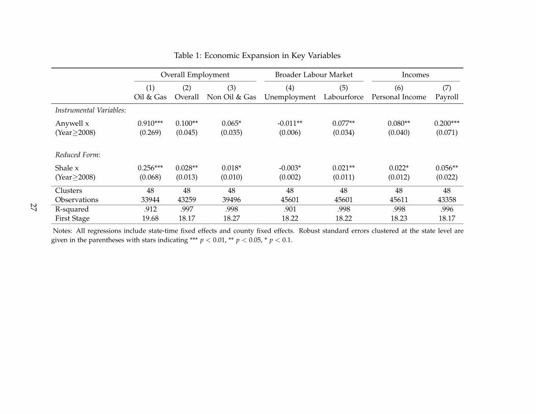
Table 1: Economic Expansion in Key Variables

Overall Employment Broader Labour Market Incomes

(1) (2) (3) (4) (5) (6) (7)Oil & Gas Overall Non Oil & Gas Unemployment Labourforce Personal Income Payroll

Instrumental Variables:

Anywell x 0.910*** 0.100** 0.065* -0.011** 0.077** 0.080** 0.200***(Year≥2008) (0.269) (0.045) (0.035) (0.006) (0.034) (0.040) (0.071)

Reduced Form:

Shale x 0.256*** 0.028** 0.018* -0.003* 0.021** 0.022* 0.056**(Year≥2008) (0.068) (0.013) (0.010) (0.002) (0.011) (0.012) (0.022)

Clusters 48 48 48 48 48 48 48Observations 33944 43259 39496 45601 45601 45611 43358R-squared .912 .997 .998 .901 .998 .998 .996First Stage 19.68 18.17 18.27 18.22 18.22 18.23 18.17

Notes: All regressions include state-time fixed effects and county fixed effects. Robust standard errors clustered at the state level aregiven in the parentheses with stars indicating *** p < 0.01, ** p < 0.05, * p < 0.1.

27

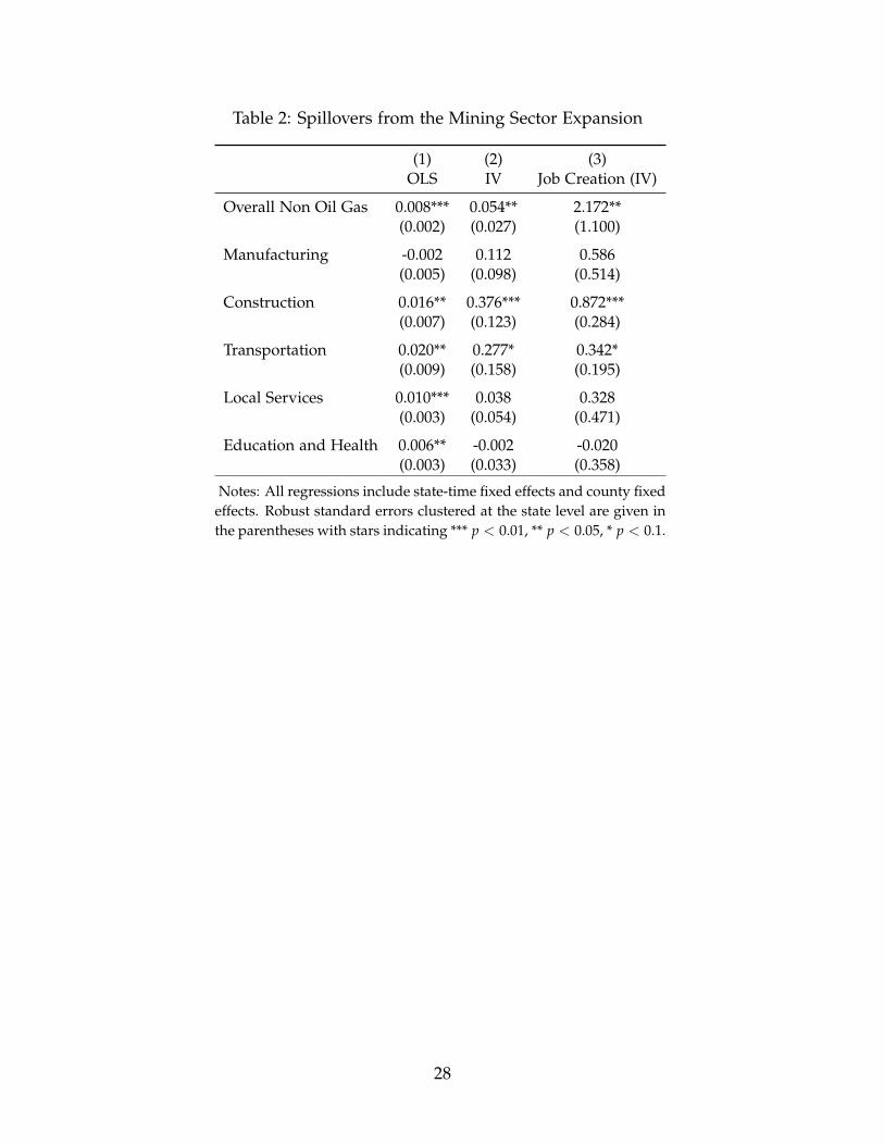
Table 2: Spillovers from the Mining Sector Expansion

(1) (2) (3)OLS IV Job Creation (IV)

Overall Non Oil Gas 0.008*** 0.054** 2.172**(0.002) (0.027) (1.100)

Manufacturing -0.002 0.112 0.586(0.005) (0.098) (0.514)

Construction 0.016** 0.376*** 0.872***(0.007) (0.123) (0.284)

Transportation 0.020** 0.277* 0.342*(0.009) (0.158) (0.195)

Local Services 0.010*** 0.038 0.328(0.003) (0.054) (0.471)

Education and Health 0.006** -0.002 -0.020(0.003) (0.033) (0.358)

Notes: All regressions include state-time fixed effects and county fixedeffects. Robust standard errors clustered at the state level are given inthe parentheses with stars indicating *** p < 0.01, ** p < 0.05, * p < 0.1.

28

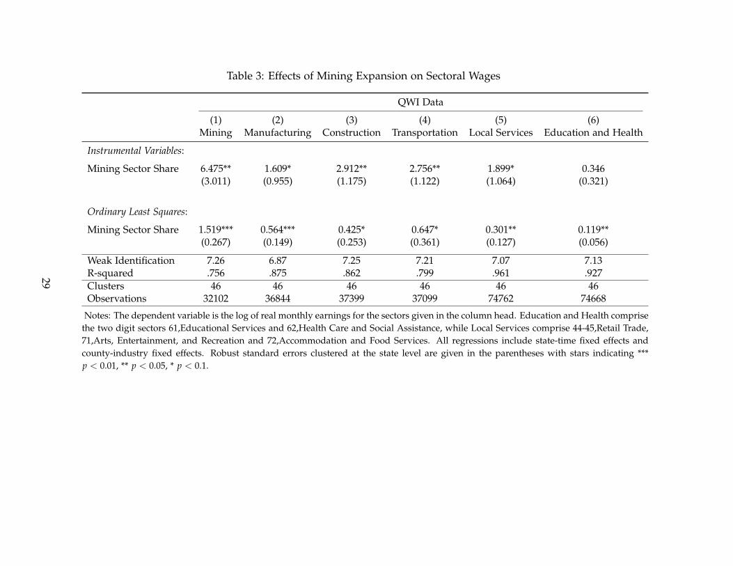
Table 3: Effects of Mining Expansion on Sectoral Wages

QWI Data

(1) (2) (3) (4) (5) (6)Mining Manufacturing Construction Transportation Local Services Education and Health

Instrumental Variables:

Mining Sector Share 6.475** 1.609* 2.912** 2.756** 1.899* 0.346(3.011) (0.955) (1.175) (1.122) (1.064) (0.321)

Ordinary Least Squares:

Mining Sector Share 1.519*** 0.564*** 0.425* 0.647* 0.301** 0.119**(0.267) (0.149) (0.253) (0.361) (0.127) (0.056)

Weak Identification 7.26 6.87 7.25 7.21 7.07 7.13R-squared .756 .875 .862 .799 .961 .927Clusters 46 46 46 46 46 46Observations 32102 36844 37399 37099 74762 74668

Notes: The dependent variable is the log of real monthly earnings for the sectors given in the column head. Education and Health comprisethe two digit sectors 61,Educational Services and 62,Health Care and Social Assistance, while Local Services comprise 44-45,Retail Trade,71,Arts, Entertainment, and Recreation and 72,Accommodation and Food Services. All regressions include state-time fixed effects andcounty-industry fixed effects. Robust standard errors clustered at the state level are given in the parentheses with stars indicating ***p < 0.01, ** p < 0.05, * p < 0.1.

29

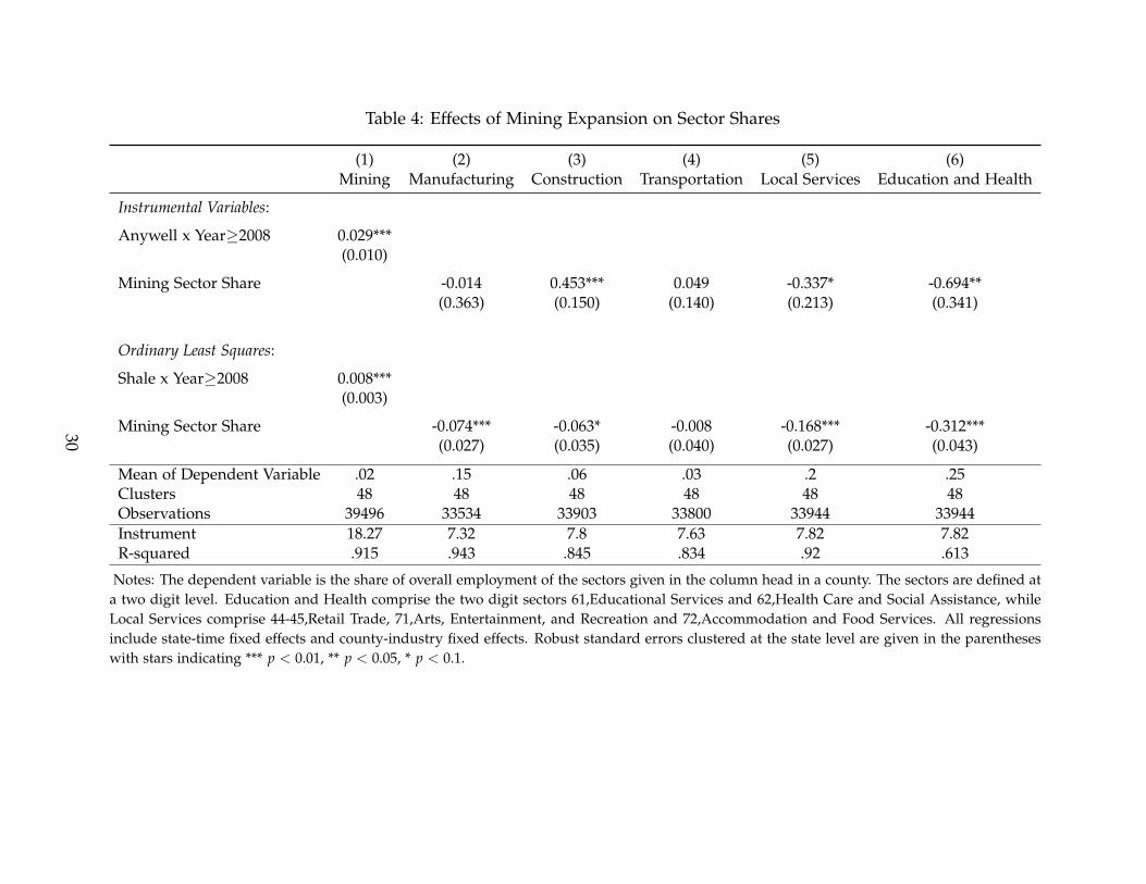
Table 4: Effects of Mining Expansion on Sector Shares

(1) (2) (3) (4) (5) (6)Mining Manufacturing Construction Transportation Local Services Education and Health

Instrumental Variables:

Anywell x Year≥2008 0.029***(0.010)

Mining Sector Share -0.014 0.453*** 0.049 -0.337* -0.694**(0.363) (0.150) (0.140) (0.213) (0.341)

Ordinary Least Squares:

Shale x Year≥2008 0.008***(0.003)

Mining Sector Share -0.074*** -0.063* -0.008 -0.168*** -0.312***(0.027) (0.035) (0.040) (0.027) (0.043)

Mean of Dependent Variable .02 .15 .06 .03 .2 .25Clusters 48 48 48 48 48 48Observations 39496 33534 33903 33800 33944 33944Instrument 18.27 7.32 7.8 7.63 7.82 7.82R-squared .915 .943 .845 .834 .92 .613

Notes: The dependent variable is the share of overall employment of the sectors given in the column head in a county. The sectors are defined ata two digit level. Education and Health comprise the two digit sectors 61,Educational Services and 62,Health Care and Social Assistance, whileLocal Services comprise 44-45,Retail Trade, 71,Arts, Entertainment, and Recreation and 72,Accommodation and Food Services. All regressionsinclude state-time fixed effects and county-industry fixed effects. Robust standard errors clustered at the state level are given in the parentheseswith stars indicating *** p < 0.01, ** p < 0.05, * p < 0.1.

30

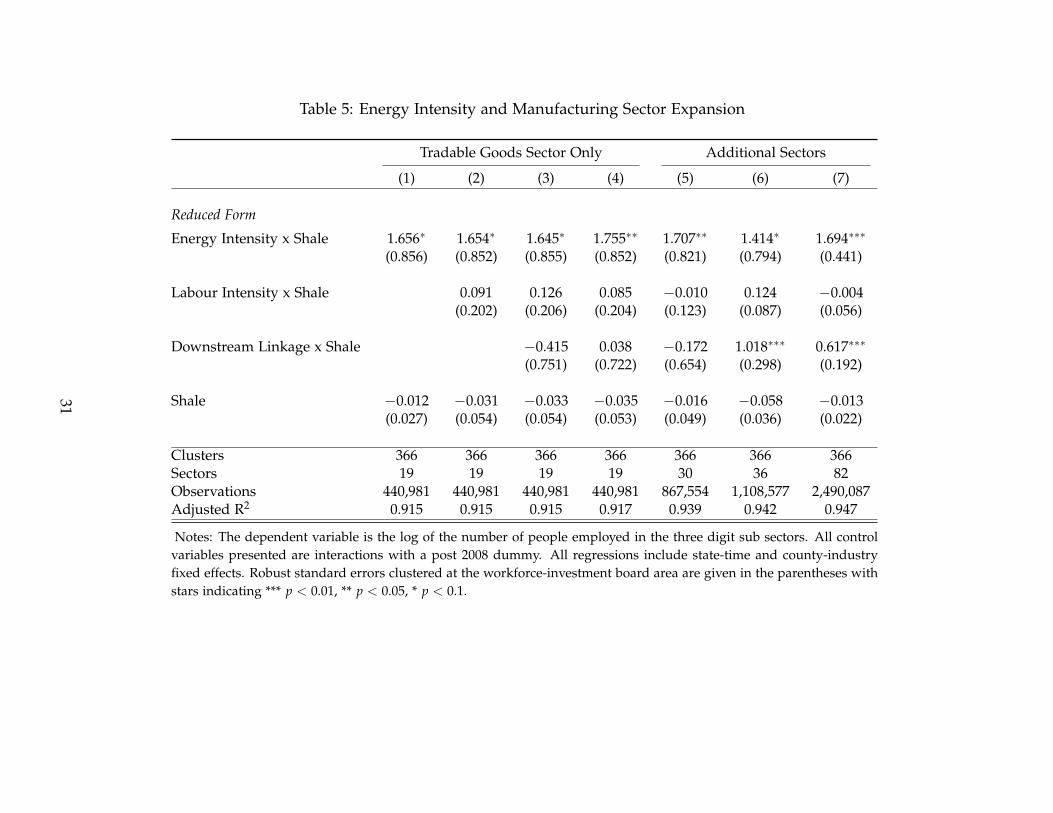
Table 5: Energy Intensity and Manufacturing Sector Expansion

Tradable Goods Sector Only Additional Sectors

(1) (2) (3) (4) (5) (6) (7)

Reduced Form

Energy Intensity x Shale 1.656∗ 1.654∗ 1.645∗ 1.755∗∗ 1.707∗∗ 1.414∗ 1.694∗∗∗

(0.856) (0.852) (0.855) (0.852) (0.821) (0.794) (0.441)

Labour Intensity x Shale 0.091 0.126 0.085 −0.010 0.124 −0.004(0.202) (0.206) (0.204) (0.123) (0.087) (0.056)

Downstream Linkage x Shale −0.415 0.038 −0.172 1.018∗∗∗ 0.617∗∗∗

(0.751) (0.722) (0.654) (0.298) (0.192)

Shale −0.012 −0.031 −0.033 −0.035 −0.016 −0.058 −0.013(0.027) (0.054) (0.054) (0.053) (0.049) (0.036) (0.022)

Clusters 366 366 366 366 366 366 366Sectors 19 19 19 19 30 36 82Observations 440,981 440,981 440,981 440,981 867,554 1,108,577 2,490,087Adjusted R2 0.915 0.915 0.915 0.917 0.939 0.942 0.947

Notes: The dependent variable is the log of the number of people employed in the three digit sub sectors. All controlvariables presented are interactions with a post 2008 dummy. All regressions include state-time and county-industryfixed effects. Robust standard errors clustered at the workforce-investment board area are given in the parentheses withstars indicating *** p < 0.01, ** p < 0.05, * p < 0.1.

31

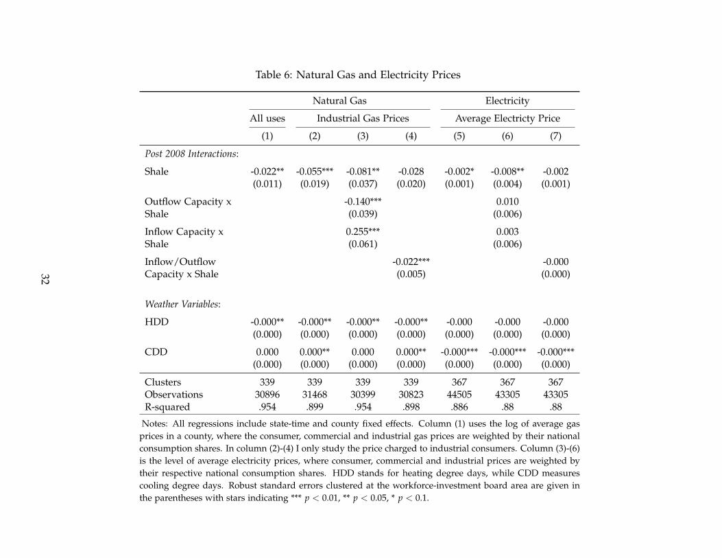
Table 6: Natural Gas and Electricity Prices

Natural Gas Electricity

All uses Industrial Gas Prices Average Electricty Price

(1) (2) (3) (4) (5) (6) (7)

Post 2008 Interactions:

Shale -0.022** -0.055*** -0.081** -0.028 -0.002* -0.008** -0.002(0.011) (0.019) (0.037) (0.020) (0.001) (0.004) (0.001)

Outflow Capacity x -0.140*** 0.010Shale (0.039) (0.006)

Inflow Capacity x 0.255*** 0.003Shale (0.061) (0.006)

Inflow/Outflow -0.022*** -0.000Capacity x Shale (0.005) (0.000)

Weather Variables:

HDD -0.000** -0.000** -0.000** -0.000** -0.000 -0.000 -0.000(0.000) (0.000) (0.000) (0.000) (0.000) (0.000) (0.000)

CDD 0.000 0.000** 0.000 0.000** -0.000*** -0.000*** -0.000***(0.000) (0.000) (0.000) (0.000) (0.000) (0.000) (0.000)

Clusters 339 339 339 339 367 367 367Observations 30896 31468 30399 30823 44505 43305 43305R-squared .954 .899 .954 .898 .886 .88 .88

Notes: All regressions include state-time and county fixed effects. Column (1) uses the log of average gasprices in a county, where the consumer, commercial and industrial gas prices are weighted by their nationalconsumption shares. In column (2)-(4) I only study the price charged to industrial consumers. Column (3)-(6)is the level of average electricity prices, where consumer, commercial and industrial prices are weighted bytheir respective national consumption shares. HDD stands for heating degree days, while CDD measurescooling degree days. Robust standard errors clustered at the workforce-investment board area are given inthe parentheses with stars indicating *** p < 0.01, ** p < 0.05, * p < 0.1.

32

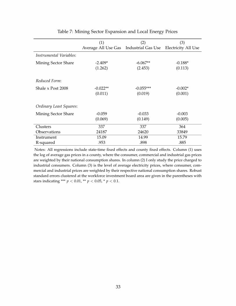
Table 7: Mining Sector Expansion and Local Energy Prices

(1) (2) (3)Average All Use Gas Industrial Gas Use Electricity All Use

Instrumental Variables:

Mining Sector Share -2.409* -6.067** -0.188*(1.262) (2.453) (0.113)

Reduced Form:

Shale x Post 2008 -0.022** -0.055*** -0.002*(0.011) (0.019) (0.001)

Ordinary Least Squares:

Mining Sector Share -0.059 -0.033 -0.003(0.069) (0.149) (0.005)

Clusters 337 337 364Observations 24187 24620 33849Instrument 15.09 14.99 15.79R-squared .953 .898 .885

Notes: All regressions include state-time fixed effects and county fixed effects. Column (1) usesthe log of average gas prices in a county, where the consumer, commercial and industrial gas pricesare weighted by their national consumption shares. In column (2) I only study the price charged toindustrial consumers. Column (3) is the level of average electricity prices, where consumer, com-mercial and industrial prices are weighted by their respective national consumption shares. Robuststandard errors clustered at the workforce investment board area are given in the parentheses withstars indicating *** p < 0.01, ** p < 0.05, * p < 0.1.

33

Appendix Tables

Table A1: Sector Specific Cost Shares

NAICS2 Sector Utility Cost Natural Gas Labour Mining Linkage1 11 Agriculture, Forestry, ... 0.020 0.004 0.120 0.0042 31-33 Manufacturing 0.053 0.042 0.192 0.2253 54 Professional, Scientific,.. 0.004 0.001 0.450 0.1024 55 Management of Companies 0.007 0.001 0.524 0.1275 44-45 Retail Trade 0.014 0.001 0.378 0.0006 61 Educational Services 0.038 0.017 0.475 0.0007 62 Health Care and Social Assistance 0.008 0.001 0.508 0.0008 71 Arts, Entertainment, and Recreation 0.016 0.002 0.357 0.0009 72 Accommodation and Food Services 0.025 0.003 0.373 0.002

10 81 Other Services 0.010 0.002 0.342 0.00411 48-49 Transportation and Warehousing 0.008 0.003 0.387 0.00512 21 Mining,Oil and Gas Extraction 0.042 0.023 0.156 0.12313 22 Utilities 0.196 0.196 0.174 0.06014 23 Construction 0.004 0.001 0.380 0.07215 42 Wholesale Trade 0.006 0.001 0.377 0.00116 51 Information 0.005 0.002 0.249 0.00617 52 Finance and Insurance 0.001 0.000 0.307 0.04218 53 Real Estate and Rental and Leasing 0.017 0.001 0.087 0.21419 56 Administrative and Support ... 0.004 0.001 0.515 0.011

34

Table A2: Economic Expansion in Key Variables

Overall Employment Broader Labour Market Incomes

(1) (2) (3) (4) (5) (6) (7)Oil & Gas Overall Non Oil & Gas Unemployment Labourforce Personal Income Payroll

Shale × 1999 -0.043 0.006 0.006 0.002 -0.003 -0.004 0.001(0.038) (0.006) (0.006) (0.002) (0.003) (0.003) (0.009)

Shale × 2000 0.042 0.008 0.006 -0.003 0.013 -0.003 0.009(0.101) (0.012) (0.011) (0.002) (0.008) (0.006) (0.018)

Shale × 2001 0.078 0.013 0.012 -0.003 0.011 -0.000 0.017(0.100) (0.014) (0.014) (0.002) (0.008) (0.006) (0.017)

Shale × 2002 0.027 0.017 0.019 -0.002 0.014 0.005 0.015(0.108) (0.015) (0.014) (0.002) (0.009) (0.007) (0.019)

Shale × 2003 0.003 0.011 0.014 -0.002 0.013 -0.003 0.018(0.111) (0.016) (0.015) (0.002) (0.009) (0.006) (0.021)

Shale × 2004 0.083 0.012 0.014 -0.003 0.015 -0.003 0.018(0.127) (0.017) (0.016) (0.002) (0.010) (0.009) (0.022)

Shale × 2005 0.103 0.016 0.013 -0.003 0.015 -0.003 0.027(0.139) (0.018) (0.018) (0.002) (0.010) (0.010) (0.022)

Shale × 2006 0.198 0.022 0.017 -0.004 0.013 0.009 0.035(0.157) (0.019) (0.019) (0.003) (0.011) (0.013) (0.022)

Shale × 2007 0.233 0.021 0.014 -0.004 0.016 -0.002 0.035(0.153) (0.018) (0.017) (0.003) (0.012) (0.011) (0.021)

Shale × 2008 0.253* 0.022 0.014 -0.005 0.019* 0.012 0.047**(0.151) (0.017) (0.016) (0.003) (0.011) (0.012) (0.022)

Shale × 2009 0.297** 0.029 0.021 -0.005 0.025** 0.022 0.053**(0.145) (0.018) (0.018) (0.004) (0.012) (0.016) (0.024)

Shale × 2010 0.323** 0.040** 0.031* -0.005 0.031** 0.019 0.071**(0.149) (0.020) (0.018) (0.003) (0.014) (0.014) (0.029)

Shale × 2011 0.418*** 0.056** 0.041** -0.006** 0.038** 0.027 0.102***(0.149) (0.023) (0.020) (0.003) (0.017) (0.019) (0.035)

Shale × 2012 0.406*** 0.063** 0.045* -0.005** 0.047** 0.031 0.107**(0.153) (0.028) (0.024) (0.002) (0.022) (0.021) (0.045)

Observations 33944 43259 39496 45601 45601 45611 43358R-squared .912 .997 .998 .901 .998 .998 .996

Notes: All regressions include state-time fixed effects and county fixed effects. Robust standard errors clustered at thestate level are given in the parentheses with stars indicating *** p < 0.01, ** p < 0.05, * p < 0.1.

35

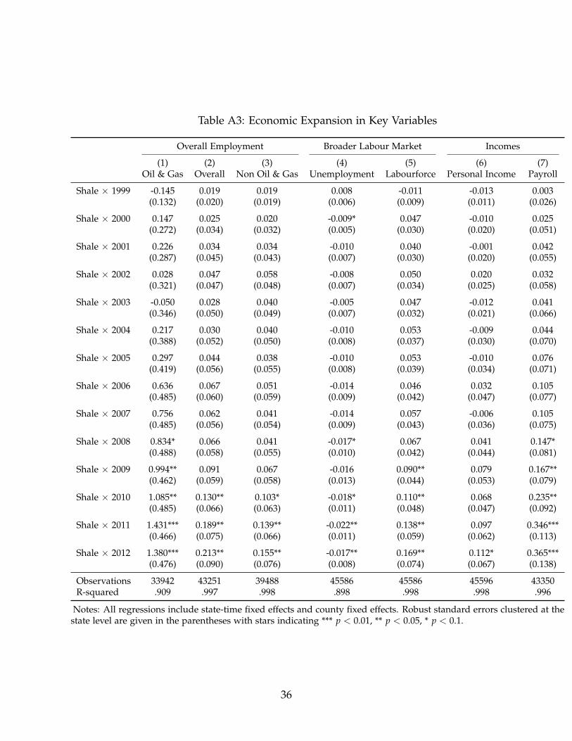
Table A3: Economic Expansion in Key Variables

Overall Employment Broader Labour Market Incomes

(1) (2) (3) (4) (5) (6) (7)Oil & Gas Overall Non Oil & Gas Unemployment Labourforce Personal Income Payroll

Shale × 1999 -0.145 0.019 0.019 0.008 -0.011 -0.013 0.003(0.132) (0.020) (0.019) (0.006) (0.009) (0.011) (0.026)

Shale × 2000 0.147 0.025 0.020 -0.009* 0.047 -0.010 0.025(0.272) (0.034) (0.032) (0.005) (0.030) (0.020) (0.051)

Shale × 2001 0.226 0.034 0.034 -0.010 0.040 -0.001 0.042(0.287) (0.045) (0.043) (0.007) (0.030) (0.020) (0.055)

Shale × 2002 0.028 0.047 0.058 -0.008 0.050 0.020 0.032(0.321) (0.047) (0.048) (0.007) (0.034) (0.025) (0.058)

Shale × 2003 -0.050 0.028 0.040 -0.005 0.047 -0.012 0.041(0.346) (0.050) (0.049) (0.007) (0.032) (0.021) (0.066)

Shale × 2004 0.217 0.030 0.040 -0.010 0.053 -0.009 0.044(0.388) (0.052) (0.050) (0.008) (0.037) (0.030) (0.070)

Shale × 2005 0.297 0.044 0.038 -0.010 0.053 -0.010 0.076(0.419) (0.056) (0.055) (0.008) (0.039) (0.034) (0.071)

Shale × 2006 0.636 0.067 0.051 -0.014 0.046 0.032 0.105(0.485) (0.060) (0.059) (0.009) (0.042) (0.047) (0.077)

Shale × 2007 0.756 0.062 0.041 -0.014 0.057 -0.006 0.105(0.485) (0.056) (0.054) (0.009) (0.043) (0.036) (0.075)

Shale × 2008 0.834* 0.066 0.041 -0.017* 0.067 0.041 0.147*(0.488) (0.058) (0.055) (0.010) (0.042) (0.044) (0.081)

Shale × 2009 0.994** 0.091 0.067 -0.016 0.090** 0.079 0.167**(0.462) (0.059) (0.058) (0.013) (0.044) (0.053) (0.079)

Shale × 2010 1.085** 0.130** 0.103* -0.018* 0.110** 0.068 0.235**(0.485) (0.066) (0.063) (0.011) (0.048) (0.047) (0.092)

Shale × 2011 1.431*** 0.189** 0.139** -0.022** 0.138** 0.097 0.346***(0.466) (0.075) (0.066) (0.011) (0.059) (0.062) (0.113)

Shale × 2012 1.380*** 0.213** 0.155** -0.017** 0.169** 0.112* 0.365***(0.476) (0.090) (0.076) (0.008) (0.074) (0.067) (0.138)

Observations 33942 43251 39488 45586 45586 45596 43350R-squared .909 .997 .998 .898 .998 .998 .996

Notes: All regressions include state-time fixed effects and county fixed effects. Robust standard errors clustered at thestate level are given in the parentheses with stars indicating *** p < 0.01, ** p < 0.05, * p < 0.1.

36

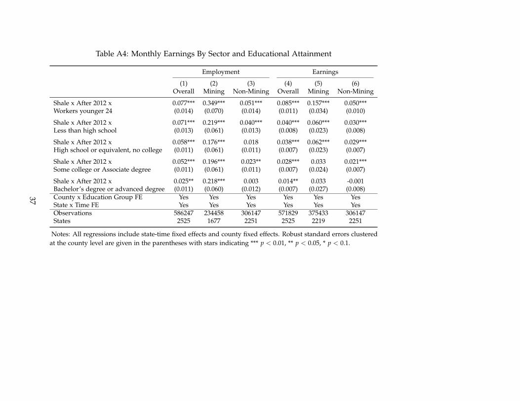
Table A4: Monthly Earnings By Sector and Educational Attainment

Employment Earnings

(1) (2) (3) (4) (5) (6)Overall Mining Non-Mining Overall Mining Non-Mining

Shale x After 2012 x 0.077*** 0.349*** 0.051*** 0.085*** 0.157*** 0.050***Workers younger 24 (0.014) (0.070) (0.014) (0.011) (0.034) (0.010)

Shale x After 2012 x 0.071*** 0.219*** 0.040*** 0.040*** 0.060*** 0.030***Less than high school (0.013) (0.061) (0.013) (0.008) (0.023) (0.008)

Shale x After 2012 x 0.058*** 0.176*** 0.018 0.038*** 0.062*** 0.029***High school or equivalent, no college (0.011) (0.061) (0.011) (0.007) (0.023) (0.007)

Shale x After 2012 x 0.052*** 0.196*** 0.023** 0.028*** 0.033 0.021***Some college or Associate degree (0.011) (0.061) (0.011) (0.007) (0.024) (0.007)

Shale x After 2012 x 0.025** 0.218*** 0.003 0.014** 0.033 -0.001Bachelor’s degree or advanced degree (0.011) (0.060) (0.012) (0.007) (0.027) (0.008)County x Education Group FE Yes Yes Yes Yes Yes YesState x Time FE Yes Yes Yes Yes Yes YesObservations 586247 234458 306147 571829 375433 306147States 2525 1677 2251 2525 2219 2251

Notes: All regressions include state-time fixed effects and county fixed effects. Robust standard errors clusteredat the county level are given in the parentheses with stars indicating *** p < 0.01, ** p < 0.05, * p < 0.1.

37

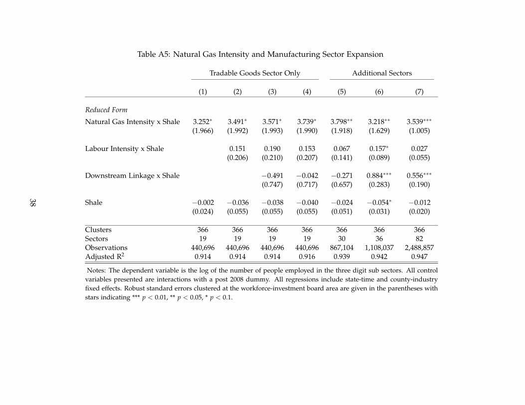
Table A5: Natural Gas Intensity and Manufacturing Sector Expansion

Tradable Goods Sector Only Additional Sectors

(1) (2) (3) (4) (5) (6) (7)

Reduced Form

Natural Gas Intensity x Shale 3.252∗ 3.491∗ 3.571∗ 3.739∗ 3.798∗∗ 3.218∗∗ 3.539∗∗∗

(1.966) (1.992) (1.993) (1.990) (1.918) (1.629) (1.005)

Labour Intensity x Shale 0.151 0.190 0.153 0.067 0.157∗ 0.027(0.206) (0.210) (0.207) (0.141) (0.089) (0.055)

Downstream Linkage x Shale −0.491 −0.042 −0.271 0.884∗∗∗ 0.556∗∗∗

(0.747) (0.717) (0.657) (0.283) (0.190)

Shale −0.002 −0.036 −0.038 −0.040 −0.024 −0.054∗ −0.012(0.024) (0.055) (0.055) (0.055) (0.051) (0.031) (0.020)

Clusters 366 366 366 366 366 366 366Sectors 19 19 19 19 30 36 82Observations 440,696 440,696 440,696 440,696 867,104 1,108,037 2,488,857Adjusted R2 0.914 0.914 0.914 0.916 0.939 0.942 0.947

Notes: The dependent variable is the log of the number of people employed in the three digit sub sectors. All controlvariables presented are interactions with a post 2008 dummy. All regressions include state-time and county-industryfixed effects. Robust standard errors clustered at the workforce-investment board area are given in the parentheses withstars indicating *** p < 0.01, ** p < 0.05, * p < 0.1.

38

A Data Appendix

A.1 Oil and Gas Well Data

Wyoming Data on horizontal wells that are mainly used for fracking purposeswere obtained upon request fromthe Wyoming Oil and Gas Conservation Commis-sion (WOGCC).16 It contains data on 1541 wells; the date on which a well was firstdug is used to construct an annual panel of active wells.

West Virginia Data on gas well drilling permits for the Marcellus Shale andUtica Shale permits issued by the West Virginia Department of Environmental Pro-tection. 17 It contains data on 3,176 permits for drilling that were issued up to May2013 commencing in 2005. The time variable used is the date the permit was issued.

Utah Data on gas and oil wells constructed were obtained from the Division ofOil, Gas and Mining - Department of Natural Resources.18 It contains data on32,176 wells completed since the 1950s. The paper uses data on unconventionalhorizontally drilled wells, the time variable is the date the well was completed.

South Dakota Data on gas and oil wells exploring shale deposits were obtainedfrom the Minerals Mining Program, Division of Environmental Services, Depart-ment of Environment and Natural Resources.19 It contains data on 292 wells com-pleted since 2000. The paper uses data on unconventional horizontally drilled wells,the time variable is the date the well was spudded.

Virginia The data on horizontal wells comes from the Virginia Department ofMines, Minerals, and Energy Division of Gas and Oil and contains all horizontalwells drilled as of June 6, 2013.20 The data starts from 2007 onwards and comprises93 wells in total. The type of well (i.e. whether oil or gas is produced is provided).

Pennsylvania The data used is for unconventionally drilled wells, which typi-cally include all horizontal wells and all wells that use hydraulic fracturing. Thedata were obtained from reports filed under the Pennsylvania Oil and Gas Actwhich requires unconventional well operators to submit production reports to the

16See http://wogcc.state.wy.us/, accessed on 14.07.2013.17See http://tagis.dep.wv.gov/fogm/, accessed on 14.07.2013.18See http://oilgas.ogm.utah.gov/Data_Center/LiveData_Search/well_data_lookup.cfm, ac-

cessed on 14.07.2013.19See http://denr.sd.gov/des/og/oghome.aspx, accessed on 14.07.2013.20See http://www.dmme.virginia.gov/dgoinquiry/, accessed on 14.07.2013

39

Department of Environmental Protection.21 The data is as of December 2012 and in-cludes data from 2005 onwards. The time variable used is the date at which drillingcommences. The type of well, i.e. whether oil or gas is produced is provided.

Oklahoma Data on shale-wells obtained from the Oklahoma Corporation Com-mission through the Oklahoma Geological Survey, containing details on unconven-tional wells. It contains data on 2694 wells from 2000 onwards. The time variableused is the well-completion date, from which point onwards the well commencesproduction.

Ohio Data on shale gas well drilling for the Mascellus and the Utica Shale wereobtained from the The data contains 16 drilling sites for the Marcellus shale and367 locations for the Utica Shale as of September 2013 starting in 2006. The timevariable is the date that the permit was issued

New York Data on 63 horizontal wells from the Marcellus, Utica, and UpperDevonian were obtained from the New York State Department of EnvironmentalConservation.22 The time variable used is the date that drilling began.

New Mexico Data on 1078 wells that were hydraulically fractured between 2009and 2012 are included in the dataset. The data was obtained from the state frackingliquids disclosure. The time vasiable is the daue in which a weml was fractured.

North Dakota Data on gas wells were extracted from the North Dakota Indus-trial Commission, Oil and Gas Division and the Current Confidential Well List.23

It contains data on 7,982 wells; data from 2000 onwards is used. The time variableused is the date!the drilling of the well began.

Data on county-level oil and gas production was obtained from the Oil and GasDivision of North Dakota. Unfortunately, well-level production data is not availablein the public domain (free of charge).

Arkansas Data on shale gas well drilling for the Faye Shale was obtained fromthe Arkansas Geological Survey.24 It contains data on 5,577 permits for drilliog that

21See https://www.paoilandgasreporting.state.pa.us/publicreports/Modules/Welcome/

Agreement.aspx, accessed on 14.07.2013.22See http://www.dec.ny.gov/imsmaps/navigator/md_oil_gas.html, accessed on 14.07.2013.23See https://www.dmr.nd.gov/oilgas/, accessed on 14.07.2013.24See http://www.geology.ar.gov/fossilfuel_maps/fayetteville_play.htm, accessed on

14.07.2013.

40

were issued up to May 2013 commencing in 2001. The time variable used is thedate the permit was issued.

Louisiana Data on shale gas well drilling for the Haynesville Shale was obtainedfrom the Louisiana Department of Natural Resources.25 It cootains data on 2,451wells issued up to June 2013. The time variable used is the date when drillingbegan.

Kentucky Data on 1,447 horizontal wells were extracted from data provided bythe Kentucky Geological Survey as of July 2013. The time variable used is the datethat drilling was completed.

Kansas Data on horizontal wells piercing the Mississippian Lime Play were ob-tained from the Kansas Geological Survey as of July 2013 Data on 1,447 horizontalwells were extracted from data provided by the Kentucky Geological Survey as ofJuly 2013. The time variable used is the date that drilling was completed.

Frac Focus Disclosure Data For the remaining states I rely on a cross-sectionof data from FracFocus. This is a voluntary disclosure website, where oil and gascompanies disclose the date, time, type of liquid and location of the well that wasfracked. Clearly, this dataset is complementing the other data-sources, filling gapswhere no data was publicly available from the state level agencies.

Figure A1 plots the spatial distribution of newly constructed wells that are partof this study. The clusters for the various shale plays highlighted in ?? is veryvisible.

As the identification strategy rests on an interaction between a time fixed effectand a cross-sectional variable indicating whether a county has unconventional de-posits, I need to justify the choice of the particular year that is used as referenceyear. For the parts where I allow the effect of a county having shale resources toflexibly vary over the years, the data makes this judgement call. However, in somespecification I divide the data into two regimes, one before 2008 and one after 2008to estimate the pooled effect across these years.

In order to justify this choice, I use the data on the timing of well constructionfor the set of states for which this data is available. I can then estimate the simplenon-parametric specification and plot the coefficients over time.26

25See http://dnr.louisiana.gov/index.cfm?md=pagebuilder&tmp=home&pid=442, accessed on14.07.2013.

26The estimated specification is as in the main part of the paper, i.e.

WellConstructioncist = αci + bst + ∑i

γi × Shalec + νcist (5)

41

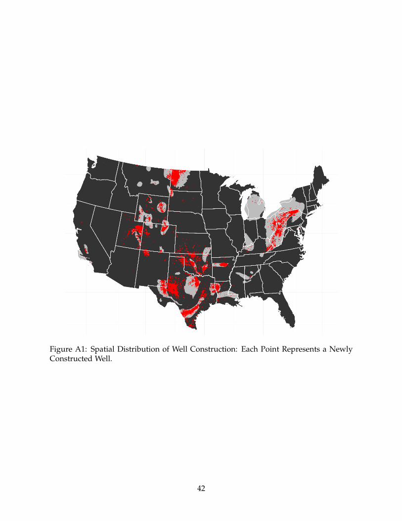
Figure A1: Spatial Distribution of Well Construction: Each Point Represents a NewlyConstructed Well.

42

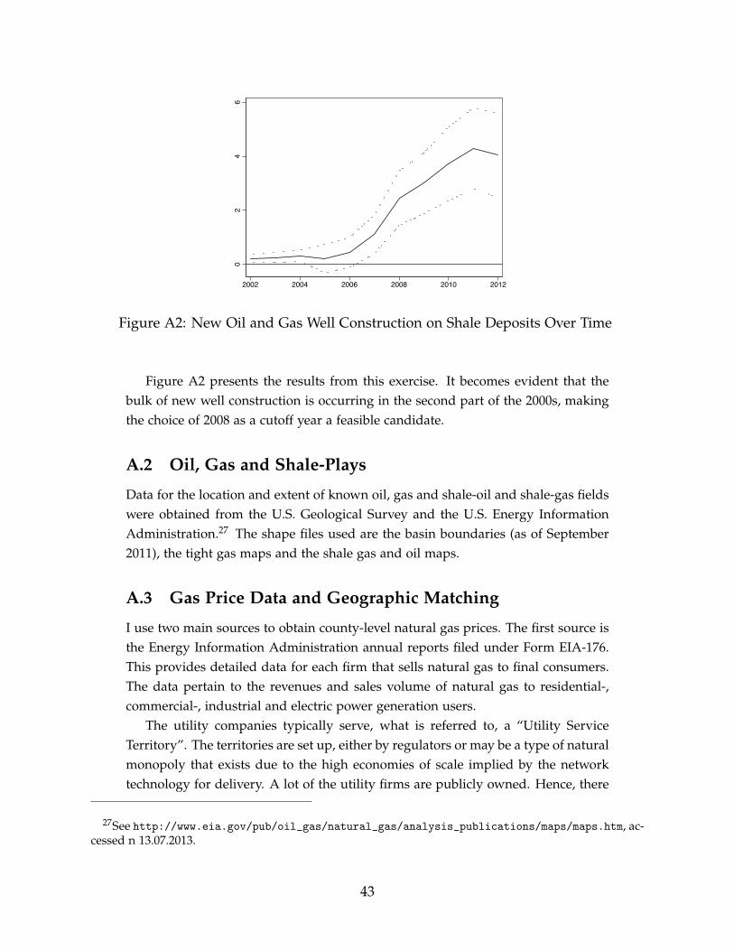
02

46

2002 2004 2006 2008 2010 2012

Figure A2: New Oil and Gas Well Construction on Shale Deposits Over Time

Figure A2 presents the results from this exercise. It becomes evident that thebulk of new well construction is occurring in the second part of the 2000s, makingthe choice of 2008 as a cutoff year a feasible candidate.

A.2 Oil, Gas and Shale-Plays

Data for the location and extent of known oil, gas and shale-oil and shale-gas fieldswere obtained from the U.S. Geological Survey and the U.S. Energy InformationAdministration.27 The shape files used are the basin boundaries (as of September2011), the tight gas maps and the shale gas and oil maps.

A.3 Gas Price Data and Geographic Matching

I use two main sources to obtain county-level natural gas prices. The first source isthe Energy Information Administration annual reports filed under Form EIA-176.This provides detailed data for each firm that sells natural gas to final consumers.The data pertain to the revenues and sales volume of natural gas to residential-,commercial-, industrial and electric power generation users.

The utility companies typically serve, what is referred to, a “Utility ServiceTerritory”. The territories are set up, either by regulators or may be a type of naturalmonopoly that exists due to the high economies of scale implied by the networktechnology for delivery. A lot of the utility firms are publicly owned. Hence, there

27See http://www.eia.gov/pub/oil_gas/natural_gas/analysis_publications/maps/maps.htm, ac-cessed n 13.07.2013.

43

Figure A3: Service Areas for Natural Gas Utility Companies.

is quite a degree of variation in the price policies. Public utilities typically holdregular public meetings in which prices are determined.

There exists no dataset at county level that provides an energy price-time seriesfor the US. However, there does exist a register of all firms involved in the natu-ral gas sector, with there annual commercial and private customer revenues andturnover.

I obtained data from the Energy Information Administration under Form EIA-176. This provides revenues and quantities of gas sold in a state and year for a localdistribution company. This allows the construction of an average price for eachutility company operating in a particular state.

I obtained non-publicly available data on utility company service areas from theEIA; the service areas can be drawn on a map, as is presented in ??. Each colourrefers to a separate utility company. It is quite obvious that some utility companiesservice huge areas, though it is unlikely that all individuals living in a particularservice area can actually be served with piped utility gas, as the service area aremost likely representing a convex hull. The map of service areas is only availablefor 2008, implying that changes in the service areas are not reflected in my data.Based on the state- by utility company average prices, I compute a county levelsimple average utility gas price.

44

A.4 Employment Data

Data on industry specific employment per quarter is obtained from the Longitudi-nal Employer-Household Dynamics dataset maintained by the US Census Bureau.In particular I use the Quarterly Workforce Indicators (QWI) that provide detailsup to 4-digit NAICS industry codes on county-level quarterly employment, payroll,earnings and job creation and destruction.

The source that feeds into the QWI is the Longitudinal Employer-HouseholdDynamics (LEHD) linked employer-employee microdata, which in turn is derivedfrom the Unemployment Insurance (UI) wage records. The data has been availablefrom the late 1990s onwards thanks to a data-sharing arrangement between theCensus Bureau and participating states.

The database roughly covers 95% of private sector employment. The core datais drawn from administrative records in the participating states and submitted oncea quarter. The QWI used here are public use products, while firm- and individuallevel data can only be physically accessed at the US Census Bureau data centres.

A concern is measurement error in the employment data due to noise-infusionor non-reporting of employment data at county level if employment in categoriesis too low. The noise-infusion is multiplicative, where the infused noise generatesnon-systematic measurement error in the employment figures, payroll and earn-ings. Abowd and Gittings (2012) show that the noise infusion does not create anysystematic bias, nor does it distort the time-series properties of the employmentdata.

More problematic are the strictly binding non-disclosure constraints which re-quire that employment counts be not reported in case there are fewer than 3 individuals-or fewer than 3 employers in a sub-geography and sector cell that contribute to thedata (Abowd (2005)).

This is particularly problematic even for employment at the 2-digit industrylevel for the mineral resource sector, as there are typically few firms operating inthis sector due to the high capital intensity.

The key binding constraint is the rigid minimum 3 employer per sector andcounty rule. For the sample I am working with, only 35.2% of the county reportemployment figures in the mining sector that are regularly distorted. 24.3% of theobservations are considered significantly distorted. The overall mean employmentfor the significantly distorted data is roughly 1/3 of the mean for the moderatelydistorted data. This hints that a significant amount of employment is not accountedfor. 40.1% of the observations do not meet the minimum disclosure condition ofthere being at least 3 employers in the county in the given sector.

This data can indirectly, but noisily, be inferred from the payroll- and earningsfigures. For 91.3 % of the non-reported employment counts, the data reports earn-

45

Figure A4: Physical Natural Gas Pipeline Net Inflow Capacity in 2002

ings and payroll. This data itself, is distorted. Since the noise-infusion is symmetricand random, the measure E f = Payroll/Earnings is a consistent estimator for theactual employment figure E∗.

Data generating process can be described as:

E∗it = φ( f (Eit))

where f is the data filter function:

f (Eit) =

1 if Eit < τ

missing if Eit ≥ τ

and φ() is the noise-infusion function.This implies a type of sample selection bias, which can be corrected for using

Heckman-style sample selection models.

A.5 Natural Gas Pipeline Network

A.6 PRISM Weather Data

In the paper I use some temperature controls to make sure that the observed varia-tion can is not attributed to weather fluctuations or trends that differentially occuron places with shale deposits. This is important as temperature in particular is adriver for the demand of energy, but may also indirectly affect economic aggregatesthrough a productivity channel.

I use the daily PRISM dataset, which provides for every day the mean, minimumand maximum temperature on a 4 by 4 kilometre grid. The data is described in

46

more detail in Daly et al. (2008). Instead of relying on reanalysis data that comes atfairly coarse resolution, the PRISM dataset relies on the dense network of weatherstations in the US; it uses 13 000 stations for precipitation and 10 000 points fortemperature every day.

Based on the daily minimum-, maximum and average temperatures, I can com-pute two measures that are often used to capture residential demand for energy:the heating degree days (HDD) and cooling degree days (CDD). This constitutesan improvement, as most papers tend to use HDD or CDD derived from aver-age temperature. This is clearly problematic, as it significantly underestimates thewithin-day variation in temperatures.

I use the formula’s developed by the UK Meterological Office, using as basetemperature T = 15 degrees centigrade. Please refer to Mourshed (2012) or Dayand Karayiannis (1999) for details. The formulas for heating degree days is givenas:

HDD =

0 if Tmin > TT−Tmin

4 if Tmin < T & Tmax+Tmin2 > T

T−Tmin2 − T−Tmin

4 if Tmin < T & Tmax+Tmin2 ≤ T & Tmax ≥ T

T − Tmin+Tmax2 if Tmin < T & Tmax+Tmin

2 ≤ T & Tmax < T

47