FQL IDE Manual

Ryan Wisnesky

April 18, 2014

Contents

1 Introduction 2

2 FQL Basics 32.1 Schemas . . . . . . . . . . . . . . . . . . . . . . . . . . . . . . . . . . . . . . . . . . . . . . . . 3

2.1.1 Cyclic Schemas . . . . . . . . . . . . . . . . . . . . . . . . . . . . . . . . . . . . . . . . 42.1.2 Enumerations (User defined types) . . . . . . . . . . . . . . . . . . . . . . . . . . . . . 52.1.3 Schema Mappings . . . . . . . . . . . . . . . . . . . . . . . . . . . . . . . . . . . . . . 52.1.4 Union Schemas and Inclusion Mappings . . . . . . . . . . . . . . . . . . . . . . . . . . 62.1.5 Schema Flow . . . . . . . . . . . . . . . . . . . . . . . . . . . . . . . . . . . . . . . . . 6

2.2 Instances . . . . . . . . . . . . . . . . . . . . . . . . . . . . . . . . . . . . . . . . . . . . . . . 72.2.1 Category of Elements . . . . . . . . . . . . . . . . . . . . . . . . . . . . . . . . . . . . 82.2.2 Relationalization and Observation . . . . . . . . . . . . . . . . . . . . . . . . . . . . . 92.2.3 Transformations (database homomorphisms) . . . . . . . . . . . . . . . . . . . . . . . 102.2.4 Instance Flow . . . . . . . . . . . . . . . . . . . . . . . . . . . . . . . . . . . . . . . . . 112.2.5 Visual Editing . . . . . . . . . . . . . . . . . . . . . . . . . . . . . . . . . . . . . . . . 11

2.3 Data Migration . . . . . . . . . . . . . . . . . . . . . . . . . . . . . . . . . . . . . . . . . . . . 112.3.1 Delta . . . . . . . . . . . . . . . . . . . . . . . . . . . . . . . . . . . . . . . . . . . . . 122.3.2 Pi . . . . . . . . . . . . . . . . . . . . . . . . . . . . . . . . . . . . . . . . . . . . . . . 122.3.3 Sigma . . . . . . . . . . . . . . . . . . . . . . . . . . . . . . . . . . . . . . . . . . . . . 142.3.4 Unrestricted Sigma . . . . . . . . . . . . . . . . . . . . . . . . . . . . . . . . . . . . . . 152.3.5 Data Migration on Transformations . . . . . . . . . . . . . . . . . . . . . . . . . . . . 152.3.6 Monads and Comonads . . . . . . . . . . . . . . . . . . . . . . . . . . . . . . . . . . . 16

2.4 Queries . . . . . . . . . . . . . . . . . . . . . . . . . . . . . . . . . . . . . . . . . . . . . . . . 182.4.1 Composition . . . . . . . . . . . . . . . . . . . . . . . . . . . . . . . . . . . . . . . . . 192.4.2 Generating Queries from Schema Correspondences . . . . . . . . . . . . . . . . . . . . 20

3 Programming with FQL 203.1 Categorical Combinators . . . . . . . . . . . . . . . . . . . . . . . . . . . . . . . . . . . . . . . 203.2 Programming with Schemas and Mappings . . . . . . . . . . . . . . . . . . . . . . . . . . . . 21

3.2.1 Co-products of Schemas . . . . . . . . . . . . . . . . . . . . . . . . . . . . . . . . . . . 213.2.2 Products of Schemas . . . . . . . . . . . . . . . . . . . . . . . . . . . . . . . . . . . . . 223.2.3 Exponentials of Schemas . . . . . . . . . . . . . . . . . . . . . . . . . . . . . . . . . . . 233.2.4 Isomorphisms of Schemas . . . . . . . . . . . . . . . . . . . . . . . . . . . . . . . . . . 24

3.3 Programming with Instances and Transformations . . . . . . . . . . . . . . . . . . . . . . . . 243.3.1 Co-products of Instances . . . . . . . . . . . . . . . . . . . . . . . . . . . . . . . . . . . 263.3.2 Products of Instances . . . . . . . . . . . . . . . . . . . . . . . . . . . . . . . . . . . . 273.3.3 Exponentials of Instances . . . . . . . . . . . . . . . . . . . . . . . . . . . . . . . . . . 283.3.4 Proposition Instances and Truth-value Transformations . . . . . . . . . . . . . . . . . 293.3.5 Isomorphisms of Instances . . . . . . . . . . . . . . . . . . . . . . . . . . . . . . . . . . 31

4 Connecting FQL with Other Systems 314.1 Compiling to SQL . . . . . . . . . . . . . . . . . . . . . . . . . . . . . . . . . . . . . . . . . . 314.2 JDBC Support . . . . . . . . . . . . . . . . . . . . . . . . . . . . . . . . . . . . . . . . . . . . 324.3 Compiling to Embedded Dependencies (EDs) . . . . . . . . . . . . . . . . . . . . . . . . . . . 334.4 Translating SQL to FQL . . . . . . . . . . . . . . . . . . . . . . . . . . . . . . . . . . . . . . . 334.5 Translating Polynomials to FQL . . . . . . . . . . . . . . . . . . . . . . . . . . . . . . . . . . 334.6 RDF Representation of Schemas and Instances . . . . . . . . . . . . . . . . . . . . . . . . . . 334.7 Converting English to FQL schemas . . . . . . . . . . . . . . . . . . . . . . . . . . . . . . . . 33

1

1 Introduction

FQL, a functorial query language, implements functorial data migration. Although functorialdata migration is formally defined using the language of category theory, it is possible tounderstand functorial data migration at the level of relational database tables. Indeed, theFQL compiler emits SQL (technically, PSM) code that can be run on any RDBMS. The FQLcompiler is hosted inside of an integrated development environment, the FQL IDE. The FQLIDE is an open-source java program that provides a code editor for and visual representationof FQL programs. A screen shot of the initial screen of the FQL IDE is shown below.

The FQL IDE is a multi-tabbed text file editor that supports saving, opening, copy-paste,etc. Associated with each editor is a “compiler response” text area that displays the SQLoutput of the FQL compiler, or, if compilation fails, an error message. The built-in FQLexamples can be loaded by selecting them from the “load example” combo box in the upper-right. In the rest of this tutorial we will refer to these examples. By default, only someexamples are shown; more can show by enabling an option. Compilation can be abortedwith the “abort” button in the Tools menu. Abort is “best effort” and can leave FQL in aninconsistent state; it is provided to allow users to terminate FQL gracefully. The FQL IDEcontains both a naive SQL engine and the H2 SQL engine; to choose which to use, see theoptions menu. In general, H2 has more overhead but performs better on large data. A codeformatter is available in the edit menu.

To run FQL with more than the default 64mb heap, you must use command line options:

java -Xms512m -Xmx2048m -jar fql.jar

2

2 FQL Basics

An FQL program is an ordered list of uniquely named declarations. Each declaration defineseither a schema, an instance, a mapping, or a query. Identifiers are case insensitive and mustbe unique. We now describe each of these concepts in turn. Comments in FQL are Javastyle, either “//” or “/* */”. Negative integers must be quoted with double quotes.

2.1 Schemas

Select the “typed employees” examples. This action will create a new tab containing thefollowing FQL code:

schema S = {

nodes

Employee,

Department;

attributes

name : Department -> string,

first : Employee -> string,

last : Employee -> string;

arrows

manager : Employee -> Employee,

worksIn : Employee -> Department,

secretary : Department -> Employee;

equations

Employee.manager.worksIn = Employee.worksIn, //1

Department.secretary.worksIn = Department, //2

Employee.manager.manager = Employee.manager; //3

}

This declaration defines a schema S consisting of two nodes, three attributes, three arrows,and three equations. In relational terminology, this means that

• Each node corresponds to an entity type. In this example, the two types of entities areemployees and departments.

• A node/entity type may have any number of attributes. Attributes correspond toobservable atoms of type int or string. In this example, each department has oneattribute, its name, and each employee has two attributes, his or her first and lastname.

• Each arrow f : X → Y corresponds to a total function f from entities of type X toentities of type Y . In this example, manager maps employees to employees, worksInmaps employees to departments, and secretary maps departments to employees.

3

• The equations specify the data integrity constraints that must hold of all instancesthat conform to this schema. FQL uses equalities of paths as constraints. A path p isdefined inductively as

p ::= node | p.arrow

Intuitively, the meaning of “.” is composition. In this example, the constraints are:1) every employee must work in the same department as his or her manager; 2) everydepartmental secretary must work for that department; and 3) there are employeesand managers, but not managers of managers, managers of managers of managers, etc.

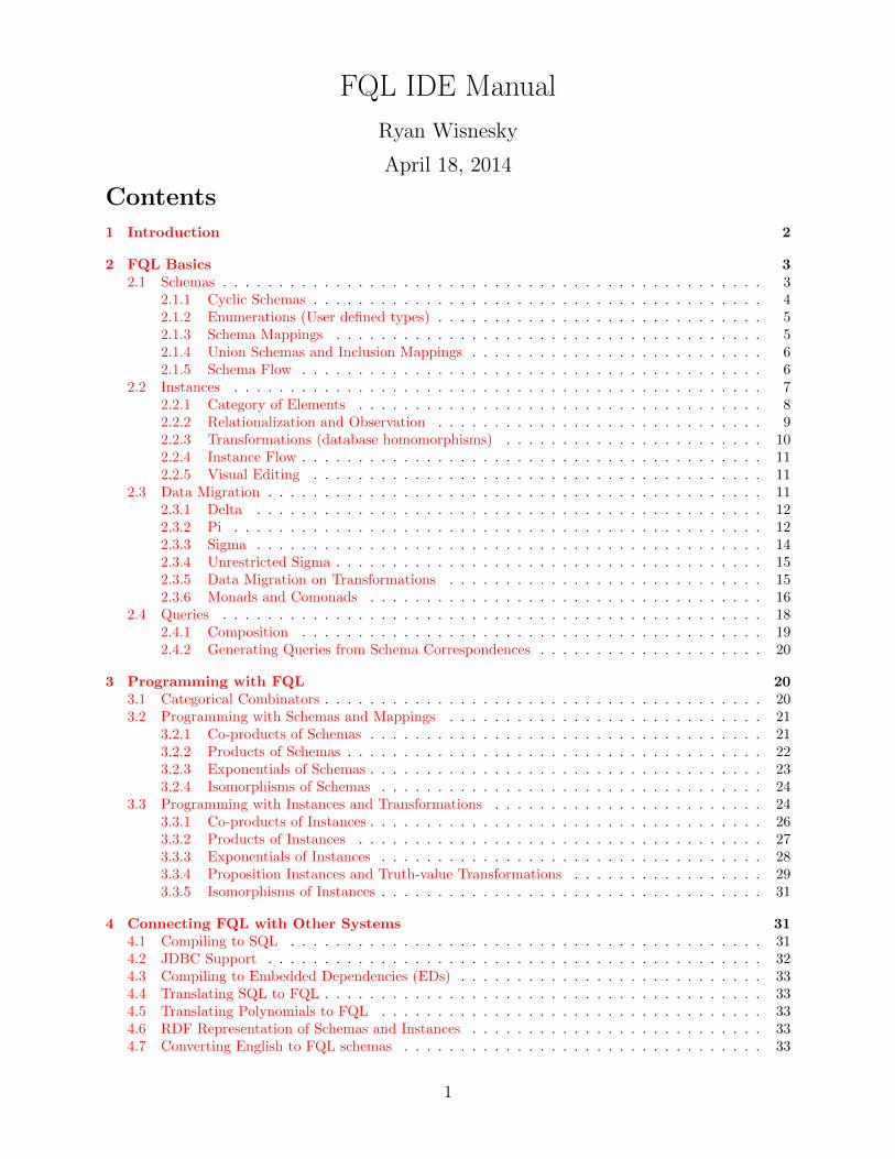
The FQL IDE can render schemas into a graphical form similar to that of an Entity-Relationship (ER) diagram. Press “compile”, and select the schema S from the viewer:

Note that the four sections, “nodes”, “attributes”, “arrows”, and “equations” are endedwith semi-colons, and must appear in that order, even when a section is empty. The “deno-tation” prints the category that the schema denotes.

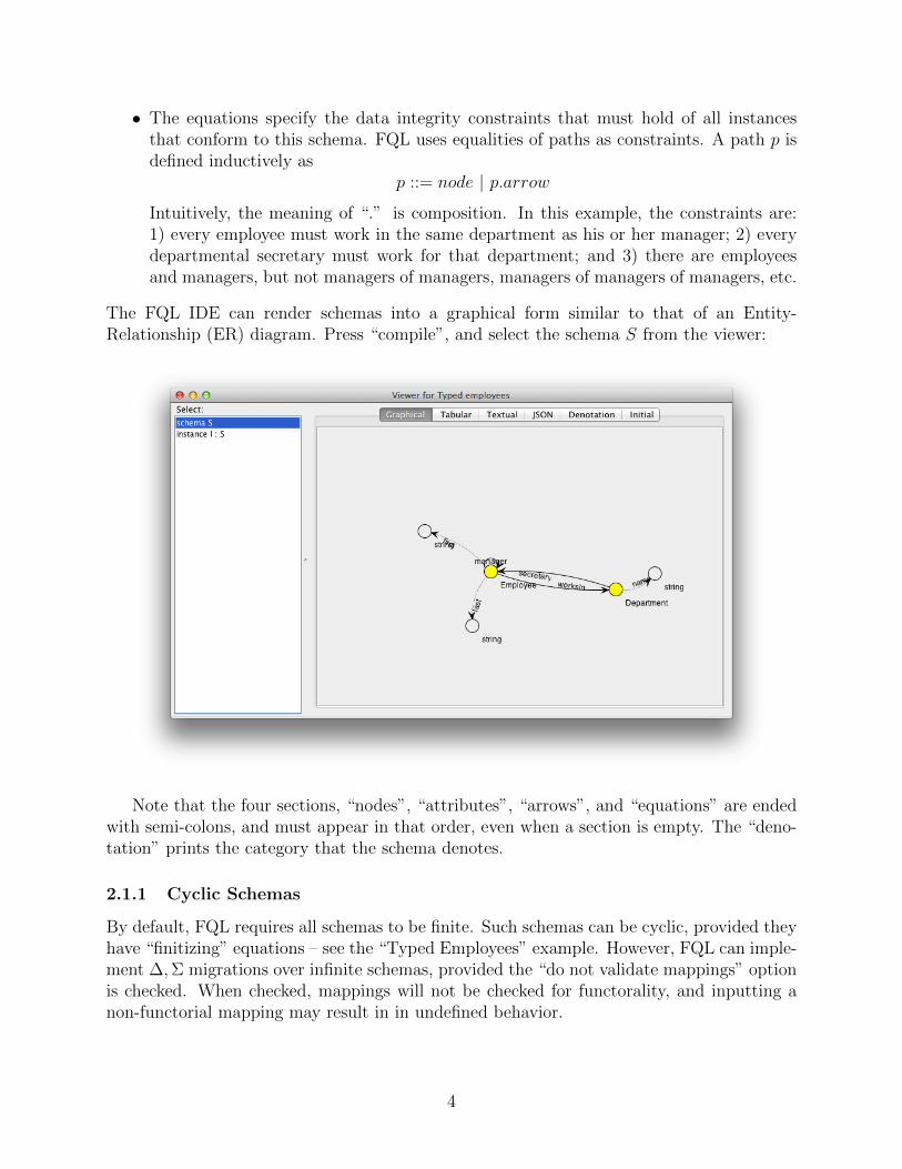
2.1.1 Cyclic Schemas

By default, FQL requires all schemas to be finite. Such schemas can be cyclic, provided theyhave “finitizing” equations – see the “Typed Employees” example. However, FQL can imple-ment ∆,Σ migrations over infinite schemas, provided the “do not validate mappings” optionis checked. When checked, mappings will not be checked for functorality, and inputting anon-functorial mapping may result in in undefined behavior.

4

2.1.2 Enumerations (User defined types)

FQL supports named enumerations. In the “Enums” example, we see:

enum color = { red, green, blue }

schema S = { nodes S_node;

attributes S_att : S_node -> color; arrows; equations; }

2.1.3 Schema Mappings

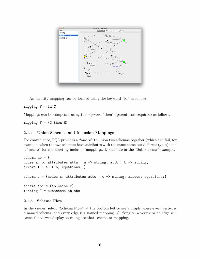
Next, load the “typed delta” example. It defines two schemas, C and D, and a mapping Ffrom C to D:

schema C = {

nodes T1, T2;

attributes

t1_ssn : T1 -> string,

t1_first : T1 -> string,

t1_last : T1 -> string,

t2_first : T2 -> string,

t2_last : T2 -> string,

t2_salary : T2 -> int;

arrows; equations;

}

→F

schema D = {

nodes T;

attributes

ssn0 : T -> string,

first0 : T -> string,

last0 : T -> string,

salary0 : T -> int;

arrows; equations;

}

mapping F = {

nodes T1 -> T, T2 -> T;

attributes

t1_ssn -> ssn0, t1_first -> first0, t1_last -> last0,

t2_last -> last0, t2_salary -> salary0, t2_first -> first0;

arrows;

} : C -> D

A mapping F : C → D consists of three parts:

• a mapping from the nodes in C to the nodes in D

• a mapping from the attributes in C to the attributes in D

• a mapping from the arrows in C to paths in D

A mapping must respect the equations of C and D: if p1 and p2 are equal paths in C, thenF (p1) and F (p2) must be equal paths in D. If this condition is not met, FQL will throw anexception. Our example mapping is rendered in the viewer as follows:

5

An identity mapping can be formed using the keyword “id” as follows:

mapping F = id C

Mappings can be composed using the keyword “then” (parenthesis required) as follows:

mapping F = (G then H)

2.1.4 Union Schemas and Inclusion Mappings

For convenience, FQL provides a “macro” to union two schemas together (which can fail, forexample, when the two schemas have attributes with the same name but different types), anda “macro” for constructing inclusion mappings. Details are in the “Sub Schema” example:

schema ab = {

nodes a, b; attributes atta : a -> string, attb : b -> string;

arrows f : a -> b; equations; }

schema c = {nodes c; attributes attc : c -> string; arrows; equations;}

schema abc = (ab union c)

mapping F = subschema ab abc

2.1.5 Schema Flow

In the viewer, select “Schema Flow” at the bottom left to see a graph where every vertex isa named schema, and every edge is a named mapping. Clicking on a vertex or an edge willcause the viewer display to change to that schema or mapping.

6

2.2 Instances

Continuing with the built-in “typed employees” example, we see that it also contains FQLcode that defines an instance of the schema S defined in the previous section:

instance I = {

nodes

Employee -> { 101, 102, 103 },

Department -> { q10, x02 };

attributes

first -> { (101, Alan), (102, Camille), (103, Andrey) },

last -> { (101, Turing), (102, Jordan), (103, Markov) },

name -> { (q10, AppliedMath), (x02, PureMath) };

arrows

manager -> { (101, 103), (102, 102), (103, 103) },

worksIn -> { (101, q10), (102, x02), (103, q10) },

secretary -> { (q10, 101), (x02, 102) };

} : S

This declaration defines an instance I that conforms to schema S. This means that

• To each node/entity type corresponds a set of globally unique IDs. In this example,the employee IDs are 101, 102, and 103, and the departmental IDs are q10 and x02.

• Each attribute corresponds to a function that maps IDs to atoms. In this example, wesee that employee 101 is Alan Turing, employee 102 is Camille Jordan, employee 103 isAndrey Markov, department q10 is AppliedMath, and department x02 is PureMath.

• Each arrow f : X → Y corresponds to a function that maps IDs of entity type X toIDs of entity type Y . In this example, we see that Alan Turing and Andrey Markovwork in the AppliedMath department, but Camille Jordan works in the PureMathdepartment.

FQL assumes that every node, attribute, and arrow is stored as a binary table; nodetables are stored as reflexive tables with types of the form (x, x). In addition, FQLassumes that the exact value of IDs are irrelevant, and in fact FQL will replaceour IDs “q10, x02, 101, 102” and “103” with generated IDs 1,2,3,4,5. Indeed,replacement of IDs will happen often with FQL data migration operations. Tovisualize this instance, press “compile”, select the instance from the viewer list, and clickthe “tabular” tab:

7

To enter a string that contains spaces, simply quote it. The ASWRITTEN keyword canautomatically generate attributes based on node IDs (see “Written macro” example).

2.2.1 Category of Elements

Provided the “Elements” option is enabled, the “Elements” tab in an instance displaysthe instance as a category, “the category of its elements”. In this view, nodes are entitiesand arrows are foreign-key correspondences. Th Elements view is well illustrated using the“People” example:

8

2.2.2 Relationalization and Observation

Associated with each type of entity in an instance is an “observation table”. For an entitytype/node N , the observation table joins together all attributes reachable by all paths outof N . Consider the “relationalize” example:

schema C={

nodes A;

attributes a:A->string;

arrows f:A->A;

equations A.f.f.f.f=A.f.f; }

instance I:C={

nodes A->{1,2,3,4,5,6,7};

attributes a->{(1,1),(2,2),(3,3),(4,1),(5,5),(6,3),(7,5)};

arrows f->{(1,2),(2,3),(3,5),(4,2),(5,3),(6,7),(7,6)}; }

instance RelI:C=relationalize I

transform trans = RelI.relationalize

9

The operation “relationalize” will equate IDs that are not distinguished by attributes.In this example, 7 rows would collapse to 4. The transform RelI.relationalize gives themapping of the 7 rows to the 4 rows. The relationalize operation is expensive, but necessaryto faithfully implement relational projection on relations that have been encoded as functorialinstances. The observation view displays the relationalization of every instance and can beenabled in the options menu. The Observables pane is never computed via JDBC.

• If your program is taking too long to run, try disabling the observables andelements GUI panes. FQL computes all GUI panes; they are not computed lazily.

2.2.3 Transformations (database homomorphisms)

For each schema T and T -instances I,J , a transformation f : I → J is a database homomor-phism from I to J : for each node n ∈ T , fn is a constraint and attribute respecting functionfrom In IDs to Jn IDs. Transformations are illustrated in the “Transform2” example:

schema C = {

nodes A;

attributes att:A->string;

arrows f:A->A;

equations A.f.f.f=A.f.f;

}

instance I = {

nodes A->{1,2,3,4,5};

attributes att->{(1,common),(2,common),(3,common),(4,common),(5,common)};

arrows f->{(1,2),(2,3),(3,3),(4,2),(5,3)};

} : C

instance J = {

nodes A->{1,2,3};

attributes att->{(1,common),(2,common),(3,common)};

10

arrows f->{(1,2),(2,3),(3,3)};

} : C

//transform BadTransform = {

// nodes A->{(1,1),(2,2),(3,4)};

//} : J -> I

transform GoodTransform1 = {

nodes A->{(1,1),(2,2),(3,3)};

} : J -> I

transform GoodTransform2 = {

nodes A->{(1,1),(2,2),(3,3),(4,1),(5,2)};

} : I -> J

The viewer for transforms is similar to the “Elements” viewer instances, except that IDsare colored according to their corresponding nodes.

2.2.4 Instance Flow

In the viewer, select “Instance Flow” at the bottom left to see a graph where every vertex isa named instance, and every edge is a data migration operation. Clicking on a vertex or anedge will cause the viewer display to change to that instance or data migration. Note thatsome data migration operations may not be explicitly named; in this case, the operation willstill display, but the operation cannot be selected by the list of named FQL declarations.

2.2.5 Visual Editing

Instances (and Transforms) can be editing using a graphical, tabular interface similar to howinstances are rendered. To visually edit an instance (transform), right-click on an instance(transform) in the main text editor and select “visually edit”. A modal dialog will pop up;by clicking on a node, the joined view of that node appears. Double-clicking in a cell allowsto change the contents of the cell; enter finalizes the change. Rows can be selected using theshift key. Note that instances (transforms) need not be well-formed to be edited, althoughthe FQL program must parse and the schema of the instance must be well-formed. Instances(transforms) can be edited in such a way that they output non well-formed FQL. Emptyvalues in cells are treated as empty strings.

2.3 Data Migration

Associated with a mapping F : C → D are three data migration operators:

• ∆F , taking D instances to C instances, roughly corresponding to projection

• ΠF , taking C instances to D instances, roughly corresponding to join

• ΣF , taking C instances to D instances, roughly corresponding to union

11

In general, certain restrictions must be placed on F to guarantee the above operationsexist. We now describe each in turn.

2.3.1 Delta

Continuing with the “typed delta” example, we see that the FQL program also defines aD-instance J , and computes I := ∆F (J):

instance I = delta F J

Graphically, we have

In effect, we have projected the columns salary0 and last0 from J .

2.3.2 Pi

Load the “typed pi” example:

12

schema C = {

nodes

c1,

c2;

attributes

att1 : c1 -> string,

att2 : c1 -> string,

att3 : c2->string;

arrows;

equations;

}

→F

schema D = {

nodes

d;

attributes

a1 : d -> string,

a2 : d -> string,

a3 : d -> string;

arrows;

equations;

}

mapping F = {

nodes c1 -> d, c2 -> d;

attributes att1 -> a1, att2 -> a2, att3 -> a3;

arrows;

} : C -> D

This example defines an instance I : C and computes J := ΠF (I):

instance J = pi F I

Graphically, this is rendered as:

13

We see that we have computed the cartesian product of tables c1 and c2. Note that theattribute mapping part of F must be a bijection for ΠF to be defined; if this condition failsFQL will throw an exception. There is menu option to allow surjections to be used instead ofbijections; we are confident that surjections behave correctly, but haven’t proven all requisitetheorems.

2.3.3 Sigma

Load the “sigma” example:

schema C = {

nodes

a1, a2, a3, b1, b2, c1, c2, c3, c4;

attributes;

arrows

g1 : a1 -> b1,

g2 : a2 -> b2,

g3 : a3 -> b2,

h1 : a1 -> c1,

h2 : a2 -> c2,

h3 : a3 -> c4;

equations;

}

→F

schema D = {

nodes A, B, C;

attributes;

arrows

G : A -> B,

H : A -> C;

equations;

}

mapping F = {

nodes

a1 -> A, a2 -> A, a3 -> A,

b1 -> B, b2 -> B,

c1 -> C, c2 -> C, c3 -> C, c4 -> C;

attributes;

arrows

g1 -> A.G, g2 -> A.G, g3 -> A.G,

h1 -> A.H, h2 -> A.H, h3 -> A.H;

} : C -> D

This example defines an instance I : C and computes J := ΣF (I):

instance J : D = sigma F I

Graphically, this is rendered as:

14

We see that we have computed union of tables a1, a2, and a3 as A (6 rows), the union oftables b1, b2 as B (5 rows), and the union of c1, c2, c3 and c4 as C (7 rows).

2.3.4 Unrestricted Sigma

For ΣF to implementable in SQL, the functor F must satisfy the special condition of beinga discrete op-fibration, which basically means “union compatible in the sense of Codd”.Mathematically, it is possible to define Σ for any schema mapping, not just mappings thatare union-compatible. Such an unrestricted sigma is known as a “Left-hand” extension. TheFQL IDE can compute such “unrestricted” sigmas, indicated by the keyword “SIGMA” (allcaps). See the “full sigma” example for details.

Note that typed (i.e., containing attributes) full sigmas 1) can create null values if thatoption is checked (but this feature is experimental and dangerous), and 2) can fail if itwould require equating two distinct constants such as “alice” and ”bob”. Full sigma can beimplemented using EDs, and indeed, we have proved that every chase sequence of these EDscorresponds to a run of the full sigma algorithm.

2.3.5 Data Migration on Transformations

If f : I → J is a transformation, then so is ∆F (f) : ∆F (J) → ∆F (I), ΣF (f) : ΣF (I) →ΣF (J), ΠF (f) : ΠF (f) : ΠF (I) → ΠF (J), and relationalize(f) : relationalize(I) →relationalize(J). See the All Syntax example for details.

15

• Note: For a full Σ the input transform must be explicitly named. While not requiredin theory, this restriction is necessary to allow full sigma on transforms to easily workwith external SQL engines that cannot natively support full sigmas.

2.3.6 Monads and Comonads

For every F and I, there are canonical transforms return : I → ∆F (ΣF (I)) and coreturn :ΣF (∆F (I)) → I, as well as canonical transforms return : I → ΠF (∆F (I)) and coreturn :∆F (ΠF (I)) → I. These transforms come from the mathematical theory of monads. Theyare illustrated in the Sigma and Pi examples, but here we will focus on the “ConnectedComponents” example. To load it, you must enable “all examples” in the options menu.The basic idea is that these transforms provide a connection between I and ΣF (I), andbetween ΠF (I) and I.

schema Graph = {

nodes arrow,vertex;

attributes;

arrows src:arrow->vertex,tgt:arrow->vertex;

equations;

}

//has 4 connected components

instance G = {

nodes arrow->{a,b,c,d,e}, vertex->{t,u,v,w,x,y,z};

attributes;

arrows

src->{(a,t),(b,t),(c,x),(d,y),(e,z)},

tgt->{(a,u),(b,v),(c,x),(d,z),(e,y)};

} : Graph

schema Terminal = {

nodes X;

attributes;

arrows;

equations;

}

mapping F = {

nodes arrow->X, vertex->X;

attributes;

arrows src->X, tgt->X;

} : Graph -> Terminal

//has 4 rows

instance Components=SIGMA F G

16

//puts 4 rows into vertex, 4 rows into arrow, corresponding to the connected components

instance I = delta F Components

//gives the transform from the original graph to the connected components

transform t = I.return

In this example, instances on schema Graph are representations of (directed) (multi)graphs: instance G contains 7 vertices and 5 edges. Running the example, we see thatComponents has 4 elements:

//instance G

{

nodes

arrow -> { 1, 2, 3, 4, 5 },

vertex -> { 6, 7, 8, 9, 11, 10, 12 }

;

attributes

;

arrows

tgt -> { (3,10), (2,11), (5,8), (1,7), (4,6) },

src -> { (3,12), (2,12), (4,8), (5,6), (1,7) };

}

//instance Components

{

nodes X -> { 15, 14, 20, 12 };

attributes;

arrows;

}

We might wish to know which connected component each arrow and vertex is a part of.Since the connected components were computed by Σ, we can use ∆ to compute anothergraph whose arrows are vertices are the connected components. Then, the return monadoperation provides a transform from the original graph to this new graph.

//instance I

{

nodes

arrow -> { 32, 31, 30, 29 },

vertex -> { 33, 34, 35, 36 }

;

attributes

;

17

arrows

tgt -> { (31,35), (30,34), (32,36), (29,33) },

src -> { (31,35), (30,34), (32,36), (29,33) };

}

//transform t : G -> I

{nodes

arrow -> {(4,32),(5,32),(3,31),(1,30),(2,31)},

vertex -> {(11,35),(10,35),(12,35),(8,36),(7,34),(6,36),(9,33)};

}

We can see above that t associates certain arrows, such as 2 and 3 to the same connectedcomponent (31).

2.4 Queries

In SQL, unions of select-from-where clauses are the common programming idiom. In FQL,the common idiom is Σs of Πs of ∆s. Load the “composition” example:

schema S = { nodes s ; attributes; arrows; equations; }

schema T = { nodes t ; attributes; arrows; equations; }

schema B = { nodes b1,b2; attributes; arrows; equations; }

schema A = { nodes a1,a2,a3; attributes; arrows; equations; }

mapping s = { nodes b1 -> s, b2 -> s; attributes; arrows; }: B -> S

mapping f = { nodes b1 -> a1, b2 -> a2 ; attributes; arrows; } : B -> A

mapping t = { nodes a1 -> t, a2 -> t, a3 -> t ; attributes; arrows; }: A -> T

query q1 = delta s pi f sigma t

In general, a query is simply a convenient shorthand.

18

Queries may be evaluated using the keyword “eval”:

instance J = ...

instance I = eval q1 J

2.4.1 Composition

FQL includes special support for composing queries. Continuing with the “composition”example, we see that it defines another query:

schema D = { nodes d1,d2 ; attributes; arrows; equations; }

schema C = { nodes c ; attributes; arrows; equations; }

schema U = { nodes u ; attributes; arrows; equations;}

mapping u = { nodes d1 -> t, d2 -> t ; attributes; arrows;}: D -> T

mapping g = { nodes d1 -> c, d2 -> c ; attributes; arrows;}: D -> C

mapping v = { nodes c -> u ; attributes; arrows; }: C -> U

query q2 = delta u pi g sigma v

We compose our two queries as follows (parenthesis required):

query q = (q1 then q2)

FQL supports another top-level type, the QUERY, for free compositions of data migrationfunctors (i.e., not triplets). Full sigma (SIGMA) can be used with QUERY.

19

2.4.2 Generating Queries from Schema Correspondences

FQL has experimental support for generating queries from attribute correspondences (schemamatching). Because such mappings are often not discrete op-fibrations, FQL defines theseusing QUERY. Many different queries can be generated from a correspondence; these areidentified by strings. Queries can be evaluated on instances with EVAL, similarly to eval.Load the “Schema Matching” example (requires the additional examples options):

schema ab = { nodes a, b;

attributes atta : a -> string, attb : b -> string; arrows f : a -> b;

equations; }

schema c = { nodes c; attributes attc : c -> string; arrows ; equations; }

QUERY q1 = match {(atta,attc),(attb,attc)} ab c "delta sigma forward"

QUERY q2 = match {(atta,attc),(attb,attc)} ab c "delta sigma backward"

QUERY q3 = match {(atta,attc),(attb,attc)} ab c "delta pi forward"

QUERY q4 = match {(atta,attc),(attb,attc)} ab c "delta pi backward"

The viewer displays the associated data migration queries:

(SIGMA {nodes c -> right_c; attributes attc -> right_attc;

arrows;} : c ->

{nodes left_a, left_b, right_c;

attributes left_atta : left_a -> string, left_attb : left_b -> string,

right_attc : right_c -> string;

arrows left_f : left_a -> left_b; equations; }

then

delta {nodes b -> left_b, a -> left_a;

attributes attb -> left_attb, atta -> left_atta;

arrows f -> left_a.left_f;

} : ab -> { nodes left_a, left_b, right_c;

attributes

left_atta : left_a -> string, left_attb : left_b -> string,

right_attc : right_c -> string;

arrows left_f : left_a -> left_b; equations; })

3 Programming with FQL

3.1 Categorical Combinators

FQL contains programming capabilities to FQL in the guise of categorical combinators. In-tuitively, these combinators are a standard functional programming language similar to e.g.,point-free Haskell. Their semantics derives from the fact that the category of schemas andmappings is bi-cartesian closed, and for each T , the category of T -instances and their homo-morphisms is a topos. Hence, schemas and mapping can be programmed using the variable-free form of the simply-typed λ-calculus, and instances and transforms can be programmed

20

using the variable-free form of higher-order logic. The main GUI contains a type-checkermenu option.

3.2 Programming with Schemas and Mappings

Schema and mapping expressions can be freely nested:

enum color = {red, green, blue}

schema C = {nodes; attributes; arrows; equations;}

schema C1 = void

schema C2 = unit {string, int, color}

schema C3 = (C + C)

schema C4 = (C * C)

schema C5 = (C union C)

schema C6 = opposite C

schema C7 = (C ^ C)

mapping F = id C

mapping F1 = (F then F)

mapping F2 = {nodes; attributes; arrows;} : C -> C

mapping F3 = inl C C

mapping F4 = inr C C

mapping F5 = (F3 + F4)

mapping F6 = fst C C

mapping F7 = snd C C

mapping F8 = (F6 * F7)

mapping F9 = void C

mapping F10= unit {string, int, color} C

mapping F13 = subschema C C5

mapping F14 = opposite F

mapping F11= eval C C

mapping F12= curry id (C*C)

mapping F15= iso1 C C

mapping F16= iso2 C C

Given a signature C, opposite C defines the signature with all the arrows reversed, and givena mapping F : C → D, opposite F : opposite C → opposite D.

3.2.1 Co-products of Schemas

The “Co-products Schema” example illustrates co-products of schemas:

schema C = { nodes a, b; attributes att : a -> string;

arrows f : a -> b, g : a -> a; equations a.g = a; }

21

schema D = { nodes a; attributes att : a -> string; arrows ; equations ; }

schema E = (C + D)

mapping f = inl C D

mapping g = inr C D

mapping h = (f + g) // this is actually the identity!

schema X = void

mapping q = void C

schema Y = ((C + (C + C)) + void)

Schemas C and D are disjointly unioned in E := C + D: each node in C appears inC + D (albeit with an automatically generated name), and each node in D appears inC + D. Similarly, the attributes and arrows of C and D are injected into C + D. Theinjection mappings have types inl C D : C → C + D and inr C D : D → C + D. Givenmappings f : C → X and g : D → X, mapping (f + g) (parenthesis required) has typeC +D → X. Co-products obey the equations

inl; (f + g) = f inr; (f + g) = g (inl + inr) = id

All manipulations of co-product schemas must be done using inl, inr, and (+). The emptyschema is written void and for every schema C, the mapping void C : void → C is theunique (empty) map to C. The empty schema is a unit for co-products in the sense that Cand void+ C are isomorphic.

3.2.2 Products of Schemas

The “Products’ Schema’ example illustrates products of schemas:

schema S = {

nodes a, b, c;

attributes att:a->string;

arrows f:a->b, g:b->c, h:a->c;

equations a.h = a.f.g;

}

schema T = {

nodes x, y;

attributes att:x->string;

arrows u:x->y, z:x->y;

equations x.u = x.z;

}

mapping F = {

nodes x -> a, y -> c;

22

attributes att->att;

arrows u -> a.f.g, z->a.f.g;

} : T -> S

schema A = (S * T)

mapping p1 = fst S T

mapping p2 = snd S T

mapping p = (p1*p2) //is identity

schema X = unit {string}

mapping H = unit {string} T

Schemas C and D are multiplied in E := C×D: nodes in C×D are pairs (c, d) where c ∈ Cand d ∈ D, albeit with automatically generated names. Hence, the attributes and arrowsof C ×D are pairs of attributes and arrows from C and D. The projection mappings havetypes fst C D : C ×D → C and snd C D : C ×D → D. Given mappings f : X → C andg : X → D, mapping (f × g) (parenthesis required) has type X → C ×D. Products obeythe equations

(f × g); fst = f (f × g); snd = g (fst× snd) = id

All manipulations of product schemas must be done using fst, snd, and (×). The schemawith one node and one attribute for each type {t1, . . .} is written unit {t1, . . .} and forevery schema C, the mapping unit {t1, . . .} C : C → unit{t1, . . .} is the unique (collapsing)map to unit {t1, . . .}. The terminal schema is a unit for products in the sense that C andunit {t1, . . .} × C are isomorphic.

3.2.3 Exponentials of Schemas

The “Exponentials” example illustrates exponentials of schemas:

schema A = {

nodes a1, a2;

attributes;

arrows af : a1 -> a2;

equations;

}

schema B = {

nodes b1, b2, b3;

attributes;

arrows bf1 : b1 -> b2, bf2 : b2 -> b3;

equations;

}

schema S = (A^B)

23

mapping eta = curry eval A B // (= id)

mapping F = unit {} (A*B) //can use any F for beta, we choose this one

mapping beta = ( ((fst A B then curry F) * (snd A B then id B))

then eval unit {} B ) // (= F)

The nodes of (CD) (parenthesis required) are mappings D → C and the arrows of CD

are natural transformations between mappings, albeit with automatically generated names.There are no attributes in CD. There is an “evaluation” mapping eval C D : CD ×D → C,and given a mapping f : A × B → C such that A has no attributes, there is a “currying”mapping curry f : A→ CB. Exponentials obey equations

curry eval = id (proj1; f × proj2; id); eval = f

All manipulations of exponential schemas must be done using eval, curry, and (−−).

3.2.4 Isomorphisms of Schemas

If S and T are isomorphic schemas, then iso1 : S → T and iso2 : T → S will be one suchisomorphism, satisfying iso1; iso2 = id and iso2; iso1 = id. Isomorphisms are particularlyuseful to convert between schemas with auto generated names and user defined names. Forexample, suppose A × B has four nodes; because the schema is a product, the nodes willautomatically be named node1, node2, node3, node4. If C is a manually input schema withnodes name, age, date, location, then iso can be used to map between A×B and C. See the“Auto Iso” example for details (requires the “all examples” option).

3.3 Programming with Instances and Transformations

For each schema T and T -instances I,J , a transformation f : I → J is a database homomor-phism from I to J : for each node n ∈ T , fn is a constraint and attribute respecting functionfrom In IDs to Jn IDs. Transformations are The following illustrates all FQL syntax forprogramming with instances and transformations:

query q = delta F pi F sigma F

query p = (q then q)

//see Schema Matching example for available strings

QUERY Q1 = delta F

QUERY Q2 = SIGMA F

QUERY Q3 = pi F

QUERY Q4 = match {} C C "delta sigma forward"

QUERY Q5 = (Q1 then Q2)

instance I = { nodes; attributes; arrows; } : C

instance I1 = delta F I

instance I2 = pi F I

24

instance I3 = sigma F I

instance I4 = relationalize I

instance I5 = SIGMA F I

instance I8 = (I + I1)

instance I10 = (I ^ I)

instance I9 = (I10 * I)

instance I11 = unit C

instance I12 = void C

instance I13 = prop C

instance I6 = external C name

instance I7 = eval q I

instance I7x = EVAL Q1 I

transform t1 = id I

transform t2 = (t1 then t1)

transform t3 = {nodes;} : I -> I

transform t4 = I8.inl

transform t5 = I8.inr

transform t6 = I8.(t4+t5)

transform t7 = I9.fst

transform t9 = I9.snd

transform t10 = I9.(t7*t9)

transform t12 = I11.unit I

transform t13 = I12.void I

transform t15 = delta I1 I1 id I

transform t16 = sigma I3 I3 id I

transform t20 = SIGMA I5 I5 t1

transform t17 = pi I2 I2 id I

transform t18 = relationalize I4 I4 id I

transform t19 = I4.relationalize

transform t21 = external I6 I6 name

transform t22 = I9.eval

transform t23 = I10.curry t22

transform t24 = iso1 I I

transform t25 = iso2 I I

transform t26 = I13.true I11

transform t27 = I13.false I11

transform t28 = I13.char t26

instance Is = kernel t28

transform t29 = Is.kernel

////(co)monads also work for SIGMA and pi

instance I3X = delta F I3

transform I3Xa = I3X.return

instance I1X = sigma F I1

25

transform I1Xa = I1X.coreturn

drop I t1

Note that equality for instances is nominal, meaning that instance names matter; if I := Eand J := E are two instances, then I 6= J even though I and J have the same definition.Indeed, I and J will have different GUIDs. As a result the FQL language of instances andtransformations is somewhat different than the FQL language of schemas and mappings.Transforms may be freely nested, but Instances cannot be, as they rely on effectful SQLoperations.

3.3.1 Co-products of Instances

The “Co-products” example illustrates co-products of instances (of the same schema):

schema S = {

nodes a, b;

attributes att : a -> string;

arrows f : a -> b;

equations;

}

instance I = {

nodes a -> {1,2}, b -> {3};

attributes att -> {(1,one),(2,two)};

arrows f -> {(1,3),(2,3)};

} : S

instance J = {

nodes a -> {a,b,c}, b -> {d,e};

attributes att -> {(a,foo),(b,bar),(c,baz)};

arrows f -> {(a,d),(b,e),(c,e)};

} : S

instance A = (I + J)

transform K = A.inl

transform L = A.inr

transform M = A.(K + L) //is id

instance N = void S

transform O = N.void J

Instances I and J are unioned in A := I + J : each ID in I appears in A (albeit witha fresh, automatically generated name), and each ID in J appears in A. Similarly, theattributes and arrows of I and J are injected into A. The injection transformations havetypes A.inl I → A and A.inr J → A. Given transformations f : I → X and g : J → X,

26

transformation A.(f + g) (parenthesis required) has type A → X. The global unique IDassumption ensures all unions are disjoint. Co-products obey the equations

A.inl;A.(f + g) = f A.inr;A.(f + g) = g A.(A.inl + A.inr) = id

All manipulations of co-product instances must be done using inl, inr, and (+). The emptyinstance U of schema T is written U := void T and for every instance V of type T , themapping U.void V : U → V is the unique (empty) map from V . The empty instance is aunit for co-products in the sense that V and void+ V are isomorphic.

3.3.2 Products of Instances

The “Products” example illustrates products of instances (of the same schema):

schema S = {

nodes a, b;

attributes att : a -> string;

arrows f : a -> b;

equations;}

instance I = {

nodes a -> {1,2}, b -> {3};

attributes att -> {(1,common),(2,common)};

arrows f -> {(1,3),(2,3)};

} : S

instance J = {

nodes a -> {a,b,c}, b -> {d,e};

attributes att -> {(a,common),(b,common),(c,baz)};

arrows f -> {(a,d),(b,e),(c,e)};

} : S

instance A = (I * J)

transform K = A.fst

transform L = A.snd

transform M = A.(K * L) //is id

schema X = {

nodes a;

attributes;

arrows;

equations;

}

instance N = unit X

transform O = N.unit N

27

Instances I and J are joined in A := I × J : each (fresh) ID in I × J corresponds to apair of ids (i, j) with i ∈ I and j ∈ J such that the attributes of i and j match. Theattributes and arrows of I and J are multiplied into I × J . The projection transformationshave types A.fst A → I and A.snd A → J . Given transformations f : X → I andg : X → J , transformation A.(f × g) (parenthesis required) has type X → A. Productsobey the equations

A.(f × g);A.fst = f A.(f × g);A.inr = g A.(A.fst× A.snd) = id

All manipulations of product instances must be done using fst, snd, and (×). The terminalinstance U of schema T (where T has only enum (or no) attributes) is written U := unit Tand for every instance V of type T , the mapping U.unit V : V → U is the unique (collapsing)map to U . The unit instance is a unit for products in the sense that V and unit × V areisomorphic. See the “Products” example for details.

3.3.3 Exponentials of Instances

The “Exponentials” example illustrates exponentials of instances (on the same schema).Note that exponentials cannot be implemented with SQL.

schema C = {

nodes a, b;

attributes;

arrows f : a -> b;

equations;

}

instance I = {

nodes a -> {1,2,3}, b -> {4,5};

attributes;

arrows f -> {(1,4),(2,5),(3,5)};

} : C

instance J = {

nodes a -> {1,2}, b -> {4};

attributes;

arrows f -> {(1,4),(2,4)};

} : C

instance K = (J^I)

instance M = (K*I)

transform trans = M.eval

transform idx = K.curry trans //eta

28

For each c ∈ C, the IDs of (J I)(c) correspond to transformations Hc × I ⇒ J , where Hc isthe “representable instance” whose IDs at Hc(d) correspond to paths c → d. There is an“evaluation” transform eval C D : CD×D → C, and given a transform f : A×B → C, thereis a “currying” transform curry f : A→ CB. As shown in the above example, exponentialsobey the “beta” and “eta” equations:

curry eval = id (proj1; f × proj2; id); eval = f

All manipulations of exponential instances must be done using eval, curry, and (−−). Paren-thesis are required. Note that exponentials can’t be used with non-enum attributes.

3.3.4 Proposition Instances and Truth-value Transformations

The “Prop” example illustrates propositional instances (on the same schema). Note thatpropositions cannot be implemented with SQL.

/* you must disable:

* - observables, elements, rdf for instances

* - graph for transforms

*/

enum dname = {AppliedMath, PureMath}

enum fname = {Alan, Camille, Andrey}

schema S = {

nodes

Employee, Department;

attributes

name : Department -> dname,

first : Employee -> fname;

arrows

manager : Employee -> Employee,

worksIn : Employee -> Department,

secretary : Department -> Employee;

equations

Employee.manager.worksIn = Employee.worksIn,

Department.secretary.worksIn = Department,

Employee.manager.manager = Employee.manager;

}

instance J = {

nodes

Employee -> { 101, 102, 103 },

Department -> { q10, x02 };

attributes

first -> { (101, Alan), (102, Camille), (103, Andrey) },

29

name -> { (q10, AppliedMath), (x02, PureMath) };

arrows

manager -> { (101, 101), (102, 102), (103, 103) },

worksIn -> { (101, q10), (102, x02), (103, q10) },

secretary -> { (q10, 101), (x02, 102) };

} : S

instance I = {

nodes

Employee -> { 101, 102 },

Department -> { q10, x02 };

attributes

first -> { (101, Alan), (102, Camille) },

name -> { (q10, AppliedMath), (x02, PureMath) };

arrows

manager -> { (101, 101), (102, 102) },

worksIn -> { (101, q10), (102, x02) },

secretary -> { (q10, 101), (x02, 102) };

} : S

transform t = {

nodes

Employee -> { (101,101), (102,102) },

Department -> { (q10,q10), (x02,x02) }

;

} : I -> J

instance prp = prop S

instance one = unit S

transform tru = prp.true one // true

transform fals = prp.false one // false

transform char_t = prp.char t

//these two transforms are equal

transform lhs = (t then char_t)

transform rhs = (one.unit I then tru)

instance ker = kernel char_t

transform char_t2 = ker.kernel

//I and ker are isomorphic

transform iso = iso1 I ker

transform should_equal_t = (iso then char_t2) //= t

30

For every schema S, there is a “proposition instance” propS, where the elements ofpropS(c) correspond to the sub-instances of Hc, where Hc is the “representable instance”whose IDs at Hc(d) correspond to paths c → d. In addition, there are “truth values”,true : 1⇒ prop and false : 1⇒ prop, where 1 is the unit instance on S. Finally, there is a“characteristic function” chi f : J ⇒ prop where f : I ⇒ J . This satisfies the equation

f ; chi f = 1; true

In addition, there is an inverse operation to chi, called kernel. If f : B ⇒ prop, thenz := kernel f is an instance, and z.kernel is a transform z ⇒ B. Note that propositionscan’t be used with non-enum attributes, and that propositional instances can be very large,often necessitating the need to disable certain gui features.

Finally, note that FQL also provides transforms for propositional logic: if X = prop S,then X.not : X ⇒ X, and if Y = X × X, then Y.and : Y ⇒ X, Y.or : Y ⇒ X, andY.implies : Y ⇒ X. See the Prop example for details.

3.3.5 Isomorphisms of Instances

If S and T are isomorphic instances (on a common schema), then iso1 : S ⇒ T and iso2 : T ⇒S will be one such isomorphism (a transform), satisfying iso1; iso2 = id and iso2; iso1 = id.See the “Auto Iso” example for details (requires the “all examples” option).

4 Connecting FQL with Other Systems

4.1 Compiling to SQL

The FQL compiler emits (very naive) SQL code that implements the FQL program. In fact,the FQL IDE executes the generated SQL to populate the viewer. The generated SQL maysimply be copied into a command-line RDBMS top-level. For example, it can by executedby “mysql embedded”. However, to use the generated SQL correctly, note the following:

• In mySQL, certain column names are not allowed, such as “left” and “right”.

• A binary table R of an instance I is referred to as I R. Hence, every node, attribute,and arrow in a schema must have a unique name. Names may appear in multipleschema, however.

• The “drop” command may be used to drop tables in the output SQL:

drop I t1 //any number of instance/transformation names

If given a single argument on the command line, a string, the FQL IDE will compile it toSQL and emit the compiled SQL on stdout. If given no arguments, the FQL IDE launchesits GUI.

To use pre-existing database tables (for instances or transforms) with the generated SQLoutput, CREATE TABLE commands in the generated SQL may need be suppressed using the

31

“external” keyword. This mechanism is described in more detail in the “external” example.The original GUID-ifying substitution for a manually entered instance/transform I is storedas tables I subst and I subst inv. When computing a data migration, FQL will maintain anumber of additional that are used for computing various transforms. For example, if I isthe result of a Π migration, then FQL will keep the “limit table” for I.

4.2 JDBC Support

The FQL IDE contains a SQL interpreter, but can be configured to use an external SQLengine using JDBC. To enable JDBC, select the appropriate check-box in the options menu,and input the Java class name of your JDBC driver, as well as the URL to your databaseinstance. Henceforth, the FQL IDE should behave exactly as before, except that it will sendits emitted SQL to the external database, and query the external database to populate theviewer. We have tested JDBC functionality on mySQL on mac. Key points:

• To load the JDBC driver from an external jar, you must not run java using “java -jar”.Instead, you must run “java” directly, for example:

java -cp "./mysql-connector-java-5.1.27-bin.jar:./fql3.jar" fql.FQL

• On compile, the FQL IDE sends the prelude the the engine, executes the emitted SQLcode, and then sends the postlude.

• To support FQL, the database engine must support variables in the form:

set @guid := 0

• The database to connect to is specified in the options menu. This database should beempty, save for any “external tables”. To delete and create databases in the externalengine, try:

drop database databasename;

create database databasename;

To examine the database directly, connect to it with:

use databasename;

• Most FQL programs omit “drop” statements. Hence, running the same script twice islikely to result in an error, because instances computed during execution of the FQLprogram will already exist. This can be avoided by use of the “drop” statement in theFQL program, or by creating a blank database as described above.

32

4.3 Compiling to Embedded Dependencies (EDs)

The FQL IDE can emit embedded dependencies (ED) that implement ∆ and untyped (fullor restricted) Σ migrations. The are found in the “ED” GUI panes. Π migrations cannotbe so implemented. The IDE also contains a dialog for performing the chase on the emittedEDs. Note that EDs only implement instance-level migration, not transform-level migration.

4.4 Translating SQL to FQL

SQL schemas and instances in categorical normal form (CNF) can be treated as FQL in-stances directly. To be in CNF, every table must have a primary key column called id.This column will be treated as a meaningless ID. The SQL to FQL item in the tool menutranslates CREATE TABLE and INSERT INTO statements into FQL programs. Columnsnot marked as foreign keys are treated as attributes.

Bags of tuples can be represented in FQL using an explicit active domain construction.Unions of conjunctive queries are supported, using DISTINCT and ALL for set semantics.Primary and foreign keys are not supported by this encoding. The RA to FQL item inthe tool menu translates CREATE TABLE, INSERT INTO, SELECT FROM WHERE,and UNION statements into FQL programs. WHERE clauses cannot use equality betweenconstants, only columns. UNIONs in RA are translated to co-products in FQL, althoughtheoretically UNIONS of SELECT-FROM-WHERE be translated to FQL queries - sigmasof pis of deltas.

4.5 Translating Polynomials to FQL

Consider polynomials p, q, r in variables x, y:

p := x2 + 2y3 q := x+ 3xy r := 2 + y

Let vars be the FQL schema with nodes x, y and let output be the FQL schema with nodesp, q, r. Then FQL can compute a query q that computes the polynomials. For example,let I be a vars-instance such that |Ix| = 2 and |Iy| = 1. Then |q(I)p| = 6, |q(I)q| = 8, and|q(I)r| = 4. To do this, select “Polynomials to FQL” from the “Tools” menu.

4.6 RDF Representation of Schemas and Instances

FQL schemas and instances support a natural RDF representation. In the schema viewer,see the “RDF” tab for an RDF schema; note that path equations are not supported by RDFschema, but the domains and ranges of each FQL schema edge are represented. Similarlysee the “RDF” tab in the FQL instance viewer for an RDF representation of instances.

4.7 Converting English to FQL schemas

Although not packaged into the FQL IDE because of its size, a java jar that converts englishsentences in subject-verb-object form is available from the FQL webpage. For example, ittranslates

33

A person is an animal.

A cow is an animal.

An animal has a height.

to

schema X = {

nodes

a_cow,

a_height,

a_person,

an_animal;

attributes;

arrows

has: an_animal -> a_height,

is_1: a_cow -> an_animal,

is: a_person -> an_animal;

equations;

}

34