Fourier transform basics for the Senior PhysicsLaboratory

Bill Tango

28 August 2014

1

2

Contents

1 Introduction 31.1 The Fourier series . . . . . . . . . . . . . . . . . . . . . . . . . . . . . . . 3

2 The Fourier transform 62.1 The Fourier transform for some simple functions . . . . . . . . . . . . . . 72.2 Existence and the impulse function . . . . . . . . . . . . . . . . . . . . . . 7

3 Convolution 103.1 The convolution theorem . . . . . . . . . . . . . . . . . . . . . . . . . . . 103.2 Linear systems . . . . . . . . . . . . . . . . . . . . . . . . . . . . . . . . 103.3 The autocorrelation function and power spectra . . . . . . . . . . . . . . . 12

4 Sampling 134.1 Sampled data . . . . . . . . . . . . . . . . . . . . . . . . . . . . . . . . . 134.2 The sampling theorem . . . . . . . . . . . . . . . . . . . . . . . . . . . . 144.3 Windowing, leakage and spectral resolution . . . . . . . . . . . . . . . . . 16

5 The discrete Fourier transform 185.1 Non-periodic sampling . . . . . . . . . . . . . . . . . . . . . . . . . . . . 19

6 Transforms in two or more dimensions 206.1 The Hankel transform . . . . . . . . . . . . . . . . . . . . . . . . . . . . . 206.2 Three-dimensional transforms . . . . . . . . . . . . . . . . . . . . . . . . 21

7 Some examples 227.1 The Lorentz profile . . . . . . . . . . . . . . . . . . . . . . . . . . . . . . 227.2 Fourier transform spectroscopy . . . . . . . . . . . . . . . . . . . . . . . . 23

7.2.1 Two wavelengths . . . . . . . . . . . . . . . . . . . . . . . . . . . 247.2.2 A Gaussian spectrum . . . . . . . . . . . . . . . . . . . . . . . . . 26

7.3 Amplitude-modulated signals . . . . . . . . . . . . . . . . . . . . . . . . . 26

Acknowledgements 29

References 29

Appendices 30

A Some useful theorems 30

B Real signals and the “analytic signal” (Advanced!!) 31B.1 Definition of the analytic signal . . . . . . . . . . . . . . . . . . . . . . . . 31B.2 Example: an interferometer illuminated with broadband light . . . . . . . . 32

C Sample MATLAB code for calculating the FFT 34

3

1 Introduction

It may come as a surprise to encounter the Fourier transform in a laboratory setting but infact the Fourier transform is an essential tool of modern experimental physics and engineer-ing. Many experiments in the Senior Physics Laboratory assume some familiarity with theFourier transform. These notes provide information about the Fourier transform which youmay find useful when working in the lab.

These notes emphasise practical applications of the Fourier transform and the treatmenthere is very different to what you might find in a mathematics text. Much of the materialpresented here is based on The Fourier Transform and Its Applications by Bracewell (1986);this is an excellent reference if you want to learn more about Fourier transforms.1 A modernand very comprehensive treatment of Fourier and related methods is by Boyd (2000).

A “signal” is a physical observable that is a function of some variable which is often, butnot always, time: a wave that propagates along a string or in a waveguide is an example ofa signal. An image can also be thought of as a signal; in this case the signal is the intensityI(x, y) at each point in the two-dimensional image. The Fourier transform allows us toassociate a second function with our signal; this function is called the spectrum. Both theoriginal signal and its spectrum contain the same information but represented in differentways, and the two representations give different insights into the physical system beingstudied.

Until the late 20th century there were two principal uses of Fourier methods:

• Fourier methods were (and still are) widely used in the theoretical analysis of manydifferent problems. Fourier, for example, introduced the concept of the Fourier seriesin his study of heat flow.

• In specialised instrumentation to determine the spectra of signals. In electronics theseinstruments are usually called spectrum analysers. In optics they are called spectrom-eters, spectrographs and optical spectrum analysers (OSAs).

With the development of modern digital computers it became practical to calculateFourier transforms both numerically and in “real time.” Today, Fourier methods are widelyused in many signal processing applications. It is quite common to take the Fourier trans-form of a signal, manipulate the spectrum in some way, and then take the inverse Fouriertransform to produce a “filtered” signal. As an example, software applications used forimage processing (e.g. Adobe PhotoShop, ImageJ or GIMP) employ Fourier methods forscratch and dust removal, image sharpening, etc.

1.1 The Fourier series

Let g(t) be a real function that is strictly periodic; i. e., it has the property g(t) = g(t+ T )where T is a constant (the period). The fundamental frequency of the function is f = 1/T .

1Ron Bracewell (1921–2007) was a distinguished graduate of the School of Physics. He was awarded firstclass honours in Physics and Mathematics and went on to complete a B.E. degree in Electrical Engineering.During the Second World War he worked in radar research at the CSIRO Division of Radiophysics (at the timelocated in what is now the Madsen Building). After the war he went to the Cavendish Laboratory in Cambridge,England, where he received his Ph.D. He was a pioneer of radioastronomy and eventually became the TermanProfessor of Electrical Engineering at Stanford University in California, a position he held until his death.

4

Such functions can be expanded in Fourier series. In elementary calculus the Fourier seriesis usually written in terms of the sine and cosine functions. In practice this can lead to quitecomplicated expressions when, for example, two series are multiplied together. Generallyit is easier to use the complex form of the Fourier series, which can be written

g(t) =∞∑

n=−∞cne

2πjnft (1.1)

where

cn =

1

T

∫ T/2

−T/2g(t)dt n = 0

1

T

∫ T/2

−T/2g(t)e2πjnftdt n ≥ 1

c∗|n| n ≤ 1

(1.2)

and j =√−1 (we follow electrical engineering practice and use j rather than i to avoid

confusion when the signal happens to be an electrical current, i(t)). The asterisk (∗) denotesthe complex conjugate. It is worth emphasising that although g(t) is a sum of complexexponentials it is nevertheless a real function.

The Fourier series expansion demonstrates that any periodic function is a linear super-position of exponential eigenfunctions having frequencies of ±f,±2f,±3f, . . . . The termc0 represents the average value of the function and is sometimes referred to as the “zero fre-quency” component. in the case of electrical signals it is also known as the D.C. component(D.C. = “direct current”). The requirement that c−n = c∗n ensures that g(t) is real.

-0.6

-0.4

-0.2

0

0.2

0.4

0.6

0 1 2 3 4 5 6 7 8 9 10

Figure 1.1: A square wave that has unit amplitude, mean of zero and frequency of 1 Hz.

5

For example, suppose that g(t) is a square wave with amplitude 1, a mean of zero andfrequency f0 (Fig. 1.1). It is easy to show that

g(t) =4

π

[sin 2πf0t+

1

3sin 6πf0t+

1

5sin 10πf0t+ · · ·

](1.3)

0.0

0.2

0.4

0.6

0.8

1.0

1.2

0 1 2 3 4 5 6 7 8 9 10

Normalised frequency f/f0

Am

plitu

de

Figure 1.2: The spectrum of a square wave of frequency f0 plotted against the normalisedfrequency f/f0. In this example the average value of the square wave is zero.

Eq. (1.3) can also be represented graphically. In Fig. (1.2) we plot the amplitudes ofeach harmonic as a function of the frequency. We call this the spectrum of the square wave.We can see from the spectrum, for example, that the square wave consists of odd harmonicsonly, a fact that may not be obvious from an inspection of the original waveform.

If a square wave is generated electrically and the signal passed to a spectrum analyser,the spectrum will be essentially the same as shown in Fig. (1.2). Similarly the diffractionpattern produced by a grating using monochromatic light will also look very much likeFig. (1.2).

Exercise: Use Eq. (1.3) with your favourite spreadsheet program to produce agraph of a square wave. Start first with only two terms in the series, and observewhat happens as more terms are added. The “ringing” (high frequency wiggles)that you see is called the Gibbs phenomenon. What causes the ringing?

6

2 The Fourier transform

The Fourier transform can be thought of as a generalisation of the Fourier series: it allowsus to find the spectrum of any function, not just periodic ones.2 The Fourier transform ofthe function f(t) is3

F (s) =

∫ ∞−∞

f(t)e−2πjtsdt (2.1)

Conversely, given F (s) the original function can be recovered by the inverse Fourier trans-form:

f(t) =

∫ ∞−∞

F (s)e2πjtsds (2.2)

Eq. (2.2) has a simple interpretation. The function f(t) is the linear superposition of theeigenfunctions exp{2πjst}. The coefficient F (s′) tells us “how much” the particular eigen-function exp{2πjs′t} contributes to the superposition.

Since the argument of the exponential function must be dimensionless the Fourier vari-able s will have units that are reciprocal to those of t. Thus if t has units of time (seconds),in Eqs. (2.1, 2.2) s will have units of frequency (hertz). If t has units of length (m), the unitsof s will be m−1 and in this case s is often called the spatial frequency.4

The Fourier transform is a linear operator that transforms one function, f(x), into an-other function, F (s). This operation can be written using the notation

F (s) = F{f(x)} (2.3)

f(x) = F−1{F (s)} (2.4)

The bar notation is also widely used:

f(s) =

∫ ∞−∞

f(x)e−2πjxsdx (2.5)

Both notations are often used to concisely express Fourier relations (see, for example,Eqs. 3.2–3.5).

If e(x) is an even function, i. e., e(x) = e(−x), the Fourier transform is reciprocal: ifE(s) = F{e(x)} then e(x) = F{E(s)}. Bracewell gives a comprehensive listing of theoddness and evenness properties of functions and their transforms; these are very helpfulfor qualititatively visualising transforms.

All physical signals are real. A property of the Fourier transform is that the Fouriertransform F (s) of a real function f(x) is Hermitian; i. e., F (s) = F ∗(−s) where the aster-isk denotes complex conjugation (compare with Eq. 1.2).

2Perhaps surprisingly, periodic functions such as sinx, cosx, square waves, etc. do not, strictly speaking,have Fourier transforms. See section 2.2.

3The definition of the Fourier transform is not unique. The definition given here is almost universal inengineering and laboratory practice. Other definitions are used, particularly in mathematics and theoreticalphysics.

4The spatial frequency is often expressed in units of “lines per millimetre” or something similar. Prior tothe introduction of SI in 1960 the unit of frequency was called “cycles per second” (cps) in English. “Lines permillimetre” is modelled on that old name for (temporal) frequency.

7

2.1 The Fourier transform for some simple functions

The Gaussian function eπx2

has the convenient property that it is its own Fourier transform:

F{eπx2} = eπs2

(2.6)

Using the similarity theorem (see Appendix A)

F{eπα2x2} = eπs2/α2

(2.7)

This illustrates a general property of Fourier transforms: if we increase the extent of a func-tion in “x-space” the transform becomes narrower in the Fourier domain. A simple physicalexample is the diffraction pattern produced when monochromatic light passes through asmall hole. As the hole is made smaller the diffraction pattern—which is the Fourier trans-form of the hole’s aperture function—gets larger.

A function that occurs repeatedly in Fourier analysis is the “top hat” or rectanglar func-tion defined by

rect(x) =

1 |x| < 1/21/2 |x| = 1/20 |x| > 1/2

(2.8)

Its Fourier transform isF{rect(x)} = sinc(πs) (2.9)

where

sinc(x) =sin(x)

x(2.10)

Note that sinc(0) = 1 as one can easily show from L’Hopital’s rule. Conversely,

F{sinc(πx)} = rect(s) (2.11)

Another function that is closely related to the top hat function is the triangle function,

tri(x) =

{0 |x| > 11− |x| |x| < 1

(2.12)

Its Fourier transform isF{tri(x)} = sinc2(πs) (2.13)

Note that the unit rectangle function rect(x) is nonzero in the range −1/2 < x < 1/2but the triangle function is nonzero in the range −1 < x < 1. The rectangle and trianglefunctions and their Fourier transforms are shown in Fig. 2.1.

2.2 Existence and the impulse function

A necessary condition for the transform of f(x) to exist is that the integral∫ ∞−∞|f(x)|dx

must exist. It follows that many familiar functions, like sin(2πft) and the constant functionf(x) = a, where a 6= 0, do not have Fourier transforms. However, these functions are

8

Figure 2.1: The unit rectangle and unit triangle functions are shown in the upper panel.Their Fourier transforms, sinc(πx) and sinc2(πx) are plotted in the lower panel.

mathematical abstractions. We can only observe a signal for a finite time: one sweep ofan oscilloscope trace, the time required for a digital acquisition system to acquire a signal,etc. Actual signals will always have a Fourier transform. To quote Bracewell: “Physicalpossibility is a valid sufficient condition for the existence of a transform.” To put it anotherway, “if you can measure it, it has a transform.”

Let P (t) be a periodic signal defined for −∞ < t < ∞. Although the integral of|P (t)| may not exist, we suppose that the integral of |e−at2P (t)| does. It follows that thisfunction will have a transform. Next, we allow a→∞. In all cases of physical interest, asa increases the transforms converge to a limit. We take this limit to be the Fourier transformof P (t).

When this process is carried out we find that the solution involves a new quantity calledthe impulse function.5 Loosely speaking, the impulse function δ(x) is defined so that

δ(x) =

{∞ x = 00 x 6= 0

(2.14)

5In theoretical physics this function is usually called the Dirac δ-function; P. A. M. Dirac introduced theδ-function in the context of quantum mechanics.

9

and ∫ ∞−∞

δ(x)dx = 1 (2.15)

The impulse function has a number of useful properties. If f(x) is any function of x,∫ ∞−∞

δ(x)f(x)dx = f(0) (2.16)∫ ∞−∞

δ(x− a)f(x)dx = f(a) (2.17)∫ ∞−∞

δ(x)f(x− a)dx = f(−a) (2.18)∫ x

−∞δ(ξ)dξ = H(x) (2.19)

In the last of these H(x) is the Heaviside function:

H(x) =

0 x < 01/2 x = 01 x > 0

(2.20)

Eqs. (2.16–2.18) express the “sifting” property of the δ-function.The impulse function allows us to assign Fourier transforms to several important func-

tions. In particular,

F{1} = δ(s) (2.21)

F{cos(πx)} = (1/2)[δ(s+ 1/2) + δ(s− 1/2)] (2.22)

F{sin(2πx)} = (j/2)[δ(s+ 1/2)− δ(s− 1/2)] (2.23)

F{eπjx} = δ(s− 1/2) (2.24)

Another function that is very useful is the comb function, also known as the samplingfunction. It is defined by

comb(x) =∞∑

n=−∞δ(x− n) (2.25)

Physically the comb function can be thought of as a series of equally spaced, extremelynarrow pulses. The comb function has the useful property that it is is own Fourier transform:

comb(x) = comb(s) (2.26)

10

3 Convolution

The convolution of the two functions f(x) and g(x) is the integral

f ?g =

∫ ∞−∞

f(u)g(x− u)du (3.1)

The convolution f ? g is a function of x and is known by many other names includingFaltung (German for “fold”), smoothing, blurring, smearing, etc. These names suggest thephysical significance of convolution.

3.1 The convolution theorem

The convolution theorem can be stated as follows: If f(x) has the Fourier transform F (s)and g(x) has the Fourier transform G(s), then the Fourier transform of f ?g is F (s)G(s).In other words, the Fourier transform of the convolution f ?g is equal to the product of theFourier transforms of f and g.

This theorem is the basis of much modern signal processing. If we want to filter somesignal f(x), we take its Fourier transform, multiply the transform by a suitable filteringfunction, and take the inverse Fourier transform of the result. This may seem like a round-about way of calculating the convolution, but with digital signal processing it is actuallyextremely efficient (see Section 4).

Bracewell gives several variations on the convolution theorem that can be neatly ex-pressed using the bar notation (the raised dot indicates ordinary multiplication):

f ?g = f ·g (3.2)

f ·g = f ?g (3.3)

f ·g = f ?g (3.4)

f ?g = f · g (3.5)

Convolution is also commutative, associative and distributive:

f ?g = g?f (3.6)

f ?(g?h) = (f ?g)?h (3.7)

f ?(g + h) = f ?g + f ?h (3.8)

3.2 Linear systems

Convolution is particularly associated with linear systems analysis, a powerful tool used inmany fields of physics and engineering. Let f(t) be the input to some system. The outputor response of the system, r(t), for the given input f(t) can be expressed in terms of someoperator T:

r(t) = T{f(t)} (3.9)

A system is linear if the following holds for any real input functions f(x), g(x) and allcomplex constants α, β:

T{αf(t) + βg(t)} = αT{f(t)}+ βT{g(t)} (3.10)

11

The response of a mechanical system to (small) forces is usually linear. Electrical cir-cuits (excluding digital electronics) are linear to a good approximation. Optical systems(lenses, etc.) are examples of two-dimensional linear systems.

It can be shown that the behaviour of any one-dimensional linear system can be repre-sented by some function h(t; t′) such that

r(t) =

∫ ∞−∞

f(t′)h(t; t′)dt′ (3.11)

for any input f(t). In particular, suppose the input or stimulus is a unit impulse, i.e., theDirac δ-function f(t) = δ(t− t0). From the sifting property of the δ-function the output orresponse will be

r(t) = h(t; t0) (3.12)

Because of this property the function h(t; t′) is called the impulse response function. If tis time, h(t, t′) is the response of the system at time t to an impulse at time t′. Causalityimplies that h(t, t′) = 0 when t < t′. Eq. (3.11) is known as the superposition integral: theoutput of a linear system is completely specified by its response to unit impulses.

Often the impulse response function is invariant; that is,

h(t; t′) = h(t− t′) (3.13)

If an impulse is applied to the system at t′ and the response is observed at t, invariancecondition means that the response depends only on the interval t − t′. In this case thesuperposition integral Eq. (3.11) becomes a convolution:

r(t) =

∫ ∞−∞

f(t′)h(t− t′)dt′ = f ?h (3.14)

In particular, the output due to the unit impulse δ(t− t0) will be h(t− t0).Let F (f),R(f) andH(f) be the Fourier transforms of f(t), r(t) and h(t), respectively.

ThenR(s) = H(s) · F (s) (3.15)

Thus, if we know the spectrum of the input, F (s), and the Fourier transform of the impulseresponse function,H(s), the spectrum of the output is simply the product of F (s) andH(s).

Question: Assuming that the impulse response of the system is known we can useEq. (3.15) to find the “true” input spectrum from the measured output spectrum:F (s) = R(s)/H(s). Do you see any problems with this method?

As the question suggests, “deconvolution” can be non-trivial but it is important in manybranches of science and engineering. Deconvolution methods are often used to removeaberrations and artefacts from images and are widely employed in fields such as radio as-tronomy, microscopy and national security.

12

3.3 The autocorrelation function and power spectra

The autocorrelation of a function f(x) is

f⊗f =

∫ ∞−∞

f(u)f(u+ x)du (3.16)

The autocorrelation is found by multiplying f(x) by a shifted copy of itself and integrating.6

It is easy to show that f⊗f has a maximum at x = 0.We began our discussion of the Fourier transform by discussing time-varying signals

and their associated spectra. The Fourier transform, however, is in general a complex quan-tity. The power spectrum of a signal f(t) is P (s) = |F{f(t)}|2. In many cases the “spec-tra” that we measure in the laboratory are power spectra.

The autocorrelation theorem is a useful tool in Fourier analysis: if f(x) has the Fouriertransform F (s) then its autocorrelation function f⊗f has the Fourier transform |F (s)|2. Anexample that frequently occurs in signal analysis is the autocorrelation of the unit rectanglefunction:

rect(x)⊗rect(x) = tri(x) (3.17)

and as we have seen the Fourier transform of tri(x) is indeed the square of the transform ofrect(x).

Another theorem that is useful in the context of power spectra is Rayleigh’s theorem.7

If F (s) is the Fourier transform of f(t) then∫ ∞−∞|F (s)|2ds =

∫ ∞−∞|f(t)|2dt (3.18)

Light is electromagnetic radiation and the radiation at a given point can be representedby the complex amplitude of the electric field U(x, y, z, t). Light detectors, however, canonly detect the intensity or power of the radiation field, |U(x, y, z, t)|2. Not surprisingly,the autocorrelation function plays an important role in modern optics.

6If f(x) is complex the autocorrelation is usually defined to be∫∞−∞ f

?(u)f(u+ x)du.7Also known as the Plancherel theorem or Parseval’s theorem.

13

4 Sampling

4.1 Sampled data

In real life we often have sampled data. This may be the result of circumstances beyondour control or because of the instrumentation we have chosen to measure our signal. Forexample, suppose we use an optical telescope to observe an interesting astronomical objectthat is time varying. In order to achieve a reasonable signal-to-noise ratio we must integratefor, say, 30 minutes. Thus we only obtain two data points or samples per hour. There is afurther complication: we are limited to observing at night and to certain times of the year.When we include factors such as cloudy nights and the fact that we have to compete withother astronomers for time on the telescope, the data we collect do not provide a continuousrecord of the variations of the object but are only snapshots at various times.

Most modern instrumentation is digital. In digital data acquisition the input signal (typ-ically a voltage or a current) is sampled and converted to a number that is stored in thecomputer. The device that does this is an analogue to digital converter (ADC).8 ADCssample the signal periodically. The sampling rate will depend on the ADC, the speed of thecomputer and other factors. Obviously we would like to sample at as high a rate as possibleto give an “almost continuous” record of the signal, but this produces extremely large datasets.

Whenever we sample data we lose information. Suppose we measure a signal at twosuccessive sample times tn and tn+1. In other words, we know, with a precision set bythe ADC, the values of f(tn) and f(tn+1). However, in the absence of any other a prioriknowledge we have no information about the value of f(x) in the interval tn < t < tn+1.

Sometimes we do have further information. Suppose, for example, we know that aparticular signal does not contain any frequency components higher than fhigh. In this casewe can choose a sampling rate that will recover all the information in the signal. Suchsignals are often said to be bandwidth-limited because we know that all the frequencies inits spectrum lie in the band 0 < f < fhigh.

If a signal is not bandwidth-limited there is the possibility that artefacts will appearin the data; that is, features will appear in the power spectrum that are not real, but are aconsequence of the sampling process.

As well as sampling the data we normally only observe a signal for a limited time span.For example, we may measure a signal for T seconds. If we measure the signal in the“window” −T/2 < t < T/2 we have absolutely no information about the signal outsidethe window.

The implications of sampling and windowing will be discussed in the next sections.8The use of the word “analogue” to denote a continuously varying quantity is curious. Both electrical

circuits and mechanical systems are described by ordinary differential equations (ODEs). With the developmentof operational amplifiers during World War II it became possible to quickly and easily assemble circuits thatwere “analogues” of mechanical systems in the sense that both the circuit and the mechanical system could bedescribed by the same ODE. The electronics were packaged into systems called “analogue computers” and werewidely used in mechanical engineering and other disciplines to study the behaviour of mechanical systems. Inan analogue computer voltages, resistors and capacitors were “analogues” of mechanical properties such asdisplacement, mass and restoring forces. Analogue computers became obsolete with the development of digitalcomputers, but the fact that analogue computers used continuously varying signals, unlike digital computerswhich use discrete values, led to the modern usage.

14

4.2 The sampling theorem

Let x(t) be a function with Fourier transform X(f) which is sampled every τ seconds. Thesampled signal can be written as

∞∑n=−∞

x(nτ)δ(t− nτ) = x(t)comb(t/τ) (4.1)

where we have made use of the comb function. Taking the Fourier transform and using theconvolution and similarity theorems (see Appendix A) we have

x(t)comb(t/τ) = τcomb(τf)?X(f) (4.2)

where we have also used the fact that the comb function is its own Fourier transform. Thisresult tells us that the Fourier transform of the sampled signal is periodic.

We now suppose that x(t) is bandwidth-limited; that is, X(f) = 0 for all frequenciesabove a cutoff frequency fc. Because the transform contains positive and negative frequen-cies the full width of the transform will be 2fc. There are three cases (see Fig. 4.1):

Oversampling: τ < 1/(2fc). In this case the Fourier transform consists of separate “is-lands.” Each island contains all the information needed to reconstruct the full functionx(t). In particular the island centred around zero frequency can be used to reconstructthe original function.

Critical sampling: τ = 1/(2fc). The “islands” now just touch. Again, the zero frequencyisland can be used to recover the original signal.

Undersampling: τ > 1/(2fc) The “islands” now overlap. If, for example, we use theisland centered on zero it will contain frequencies that have spilled over from adjoin-ing islands. When we reconstruct the original signal these spurious frequencies willappear as artefacts.

The process that introduces these artefacts is called “aliasing” and occurs whenever thedata are undersampled. Both movies and television pictures are sampled and fast movingobjects can show aliasing. This is why the wheels of cars, bicycles, etc. sometimes appearto stop or go backwards. Images in digital format are made up of “pixels” and images thatcontain high spatial frequencies can exhibit aliasing effects, as shown in Fig. 4.2.

There is one exceptional condition. Suppose our signal contains a periodically varyingcomponent which is exactly zero at each sample point. This frequency component is notobservable.

We can now state the Nyquist-Shannon sampling theorem: A function whose Fouriertransform is zero for |f | > fc is fully specified by values taken at equal intervals not exceed-ing 1/(2fc) except for any harmonic term with zeros at the sampling points. The frequency2fc is the Nyquist rate.9

9The Nyquist rate is not the same as the Nyquist frequency, which is defined to be fN = 1/(2τ). The twoare often confused.

Harry Nyquist (1889-1976) was a Swedish-American engineer who worked for the American telephonecompany AT&T (later to become Bell Telephone Laboratories). He made fundamental contributions to ourunderstanding of noise processes, signal theory and the stability of circuits with feedback. His name is asso-ciated with thermal noise processes (Johnson-Nyquist noise), the properties of sampled signals (the Nyquistfrequency) and the condition for the stability of circuits with negative feedback (the Nyquist criterion).

15

Figure 4.1: The sketches show the Fourier transform of a set of sampled data. The samplingfrequency, from top to bottom, is (a) oversampled, (b) critically sampled and (c) undersam-pled. In the first two cases it is possible to recover the bandwidth-limited spectrum of thedata from the sampled spectrum. In the last example the spectra overlap, creating artefacts(aliasing).

16

Figure 4.2: A computer generated image (CGI) of a tiled pavement. The image is under-sampled and this gives rise to the aliasing artefacts noticeable near the vanishing point inthis perspective render.

Well designed digital instrumentation will have “anti-aliasing” filters. For a given sam-pling period τ the anti-aliasing filter blocks all frequencies greater than 1/2τ , ensuring thatno aliasing artefacts will appear. High quality digital cameras have an optical anti-aliasingscreen directly in front of the detector array for the same purpose.

4.3 Windowing, leakage and spectral resolution

To find the Fourier transform of some function x(t) it is assumed that we know the value ofthe function for −∞ < t < ∞. For all “real world” signals we can only record them in alimited time window of duration T . To be specific, suppose we measure a signal x(t) oversome interval −T/2 < t < T/2. The “true” Fourier transform of x(t) is

X(s) =

∫ ∞−∞

x(t)e−2πjstdt (4.3)

whilst the Fourier transform of the measured signal will be

Xmeas(s) =

∫ ∞−∞

rect(t/T )x(t)e−2πjstdt (4.4)

where rect(x) is the rectangle function defined in Eq. (2.8). We can use Eq. (3.2) to writethis as

Xmeas(s) = sinc(πTs)?X(s) (4.5)

17

The Fourier transform of the measured signal is the convolution of the sinc functionwith the “true” Fourier transform. Consider, for example, a pure sine wave of frequency f0.Its (positive) spectrum will consist of a delta function at f0. If we measure it in a T secondtime window the measured spectrum will be sinc[π(f − f0)/T ] instead of δ(f − f0). Oneway of describing this phenomenon is to say that power has “leaked” from the frequency f0

into other frequencies.Windowing or leakage is particularly important when a spectrum has many closely

spaced frequency components. The measurement time T effectively determines the spec-tral resolution of the measurement process. In order to accurately measure two frequenciesseparated by ∆f it is necessary to use T � ∆f−1.

One way to minimise the effect of leakage is to use windowing functions. Rather thancalculate the spectrum using Eq. (4.4) we use

Xwind(s) =

∫ ∞−∞

W (t/T )x(t)e−2πjstdt (4.6)

where W (x) is a windowing or taper function. A window function usually has a maximumat t = 0 and falls smoothly to zero at t = ±T/2. It reduces (but does not eliminate) theeffect of leakage. There are many different functions that are used for windowing and thechoice will depend on the particular details of the measurement.

Windowing is closely associated with sampling. Suppose that we collect a finite set ofdata at times−T/2, T/2+τ , . . .T/2. Following the same argument as given in the previoussection we can write the sampled signal as

T/(2τ)∑n=−T/(2τ)

x(nτ)δ(t− nτ) = x(t)comb(t/τ)Π(t/T ) (4.7)

Without going into detail one can show that windowing has a similar effect on sampled dataas it does for continuous data.

18

5 The discrete Fourier transform

The discrete Fourier transform (DFT) is a computational procedure to determine the Fouriertransform of the lowest frequency “island” described in section 4.1. Let τ be the samplinginterval, let N be the total number of samples and set xn = x(nτ). The DFT is usuallydefined by

Xk =

N−1∑n=0

xn exp

{−2πj

Nkn

}k = 0, 1, 2, . . . , N − 1 (5.1)

The inverse transform is defined similarly:

xn = N−1N−1∑k=0

Xk exp

{2πj

Nkn

}n = 0, 1, 2, . . . , N − 1 (5.2)

The continuous Fourier transform includes both positive and negative frequencies but theDFT defined here only has positive frequencies. It is possible to define the DFT with krunning from −N/2 to N/2 (e. g., see Bracewell) but many computer languages limit sub-scripts to positive integers and the definition of the DFT given here is standard in computa-tional science.

Eq. (5.1) can be written as

Xk =N−1∑n=0

Ankxk k = 0, 1, 2, . . . , N − 1 (5.3)

whereAnk = exp{−2πjnk/N} (5.4)

The sampled data and the spectrum can be written as N-dimensional vectors:

x = (x0, x1, . . . xN−1) (5.5)

X = (X0, X1, . . . XN−1) (5.6)

and we can also define an N × N matrix A having elements given by Eq. (5.4). UsingEuler’s identity these matrix elements can be written as Ank = (ωN )nk, where ωN =exp{−2πj/N} is a primitive N th root of unity. The matrix elements are uniformly spacedon the unit circle in the complex plane. Eqs. (5.1, 5.2) can be written in the alternative form:

X = Ax (5.7)

x = N−1A−1X (5.8)

With the development of digital computers in the last century It was realised that theDFT could be used to perform numerical Fourier transforms. However it is clear fromEq. (5.3) that there are N(N + 1)/2 ∼ N2/2 multiplications required to compute the DFT.Cooley and Tukey (1965) developed an algorithm that has become known as the Fast FourierTransform (FFT). They showed that if N = 2n it was possible to calculate the transformusing only 2N log2N multiplications. This greatly reduced the time required to calculatethe transform and the FFT has ever since been the standard algorithm for computing DFTs.

19

The standard reference for numerical techniques, including the FFT, is Press et al.(2007). This text not only includes algorithms but extensive discussions of various nu-merical methods.

Just as the original signal (x0, x1, . . . , xN−1) consists of discrete or sampled pointsthe spectrum will consist of discrete frequencies. The amplitudes of these frequencies are(X0, X1, . . . XN−1), with X0 being the “zero frequency” amplitude equal to

∑N−1n=0 xn.

Let τ be the sampling interval. The sampled data will span T = Nτ seconds. The low-est non-zero frequency in the spectrum will be 1/T Hz, and in general the spectrum willconsist of the frequencies 0, 1/T, 2/T, . . . k/T, . . . (N − 1)/T . For simplicity assume thatN is even. Since the signal x is real one can show that X(k) = X∗(N − k); this is anal-ogous to the Hermitian property of the continuous Fourier transform. All the informationabout the transform is contained in the set (X0, X1, . . . , XN/2) and the highest frequencyin the DFT spectrum will be N/2T = (2τ)−1. This is also the Nyquist frequency. Thespectral resolution is 1/T = (Nτ)−1. To summarise, the sampling period τ determines thehighest frequency in the DFT/FFT and the number of samples (or the total sampling time)determines the spectral resolution.

If the sampled signal has frequency components greater than the Nyquist frequencythen aliasing artefacts can occur. It is important to emphasise that this is not caused by theDFT/FFT; it is a result of the sampling process itself. Careful design of both the measure-ment and data acquisition systems will prevent aliasing effects and ensure that the spectralresolution is sufficient to detect the signals of interest.

In many computing environments the computation of the FFT is very straightforward.See, for example, Trefethen (2000); sample MATLAB code is included in Appendix (C).

5.1 Non-periodic sampling

Under controlled laboratory conditions it is feasible to sample data at precisely fixed sam-pling rates. However when investigating phenomena in the real world this is not alwayspossible. In fields like meteorology and astronomy the sampling process can be far fromideal. The subject of non-periodic data is beyond the scope of these notes, but it is inter-esting to note that the original algorithm for dealing with non-periodic data is the Lomb-Scargle periodogram, developed by Nick Lomb when he was a Ph.D. student in the Schoolof Physics. More recently wavelet analysis is often preferred to Fourier analysis when thedata are discontinuous and not uniformly sampled. For more information about these andother methods see Press et al. (2007).

20

6 Transforms in two or more dimensions

It is possible to extend the definition of the Fourier transform to multiple dimensions. Themost widely used is the two-dimensional Fourier transform:

F (u, v) =

∫ ∞−∞

∫ ∞−∞

f(x, y)e−2πj(ux+vy)dxdy (6.1)

f(x, y) =

∫ ∞−∞

∫ ∞−∞

F (u, v)e2πj(ux+vy)dudv (6.2)

Two-dimensional systems include such diverse systems as stretched membranes, antennas,arrays of antennas, lenses, diffraction gratings and two-dimensional images. The variablesu and v are called spatial frequencies; since the quantity (ux+ vy) must be dimensionlessthe dimensions of u and v are reciprocal to the dimensions of x and y. Thus if x andy have dimensions of length u and v will have dimensions (length)−1. Virtually all thestandard theorems for Fourier transforms carry over to two dimensions and two-dimensionalanalogues of convolution, autocorrelation, etc., can be defined in the obvious way.

The relation between one- and two-dimensional transforms can be emphasised by notingthat x = (x, y) and u = (u, v) can be regarded as vectors and we can write

F (u) =

∫ ∞−∞

f(x)e−2πjx·ud2x (6.3)

f(x) =

∫ ∞−∞

F (u)e2πjx·ud2u (6.4)

The DFT and FFT can also be extended to two-dimensions. Let Nx and Ny be thenumber of samples in the x and y directions. The DFT will require∼ N2

xN2y multiplications

whilst the FFT will use ∼ NxNy log2(Nx +Ny).

6.1 The Hankel transform

Many physical systems have circular symmetry. Obvious examples are lenses and circularradio antennas. Define the circular coordinate system

r = (x2 + y2)1/2 (6.5)

θ = arctan(y/x) (6.6)

with dxdy = rdrdθ. We can define a similar coordinate system (q, φ) for the (u, v) plane.A circularly symmetric function will depend only on the variable r and it is apparent thatits Fourier transform will depend only on q. After some algebra we find that

F (q) = 2π

∫ ∞0

f(r)J0(2πqr)dr (6.7)

and similarly

f(r) = 2π

∫ ∞0

F (q)J0(2πqr)dq (6.8)

where J0(z) is the zero-order Bessel function of the first kind. These two equations definethe Hankel transform (of zero order) and its inverse.

21

6.2 Three-dimensional transforms

Three-dimensional transforms are defined in the obvious way:

F (u, v, w) =

∫ ∞−∞

∫ ∞−∞

∫ ∞−∞

f(x, y, z)e−2πj(ux+vy+wz)dxdydz (6.9)

f(x, y, z) =

∫ ∞−∞

∫ ∞−∞

∫ ∞−∞

F (u, v, w)e2πj(ux+vy+wz)dudvdw (6.10)

In physics they are most commonly encountered in the theory of X-ray diffraction fromcrystals.

22

7 Some examples

These examples have been chosen because they relate directly to various experiments in theSenior Physics Laboratory.

7.1 The Lorentz profile

The Lorentz profile occurs in many areas of atomic physics. The “natural” linewidth ofatomic spectral lines (i.e., the linewidth in the absence of Doppler motion, the effects ofneighbouring atoms, etc.) has a Lorentz profile. The resonances seen in nuclear magneticresonance, electron spin resonance and optical pumping experiments also have a Lorentzprofile.

Figure 7.1: A sketch of a damped harmonic oscillation.

In the semi-classical approximation, the excited states of atoms behave like dampeddipole oscillators. The frequency of oscillation is ν0 = ∆E/h where ∆E is the energydifference between the excited and ground states and the damping coefficient is generallydenoted by Γ (with units of s−1). The radiation v(t) from a damped oscillator decaysexponentially as shown in Fig. (7.1):10

v(t) =

{0 t < 0

Ae−Γt/2 cos(2πνt) t > 0(7.1)

We can simplify the discussion by replacing the cosine function with a complex expo-nential:

v(t) = AH(t)e2πjνte−Γt/2 (7.2)10The damping coefficient is defined so that Γ−1 is the time required for the radiated power to fall by a factor

of e. The power is proportional to |v(t)|2 and this is the reason for the facttor of 2 in Eq. (7.1).

23

We have also used the Heaviside function H(t) to simplify the notation. The spectrum ofv(t) is found from its Fourier transform:

S = A

∫ ∞0

e−Γt/2e−2πj(ν−ν0)tdt

=2A

Γ

∫ ∞0

e−xe−4πj(ν−ν0)x/Γdx

=A

Γ

∫ ∞0

e−xe−2πjsxdx (7.3)

where s = 2Γ−1(ν − ν0). Eq. (7.3) is the Fourier transform of H(x)e−|x| and can be foundfrom tables of Fourier transforms:

S(s) =2A

Γ

1− 2πjs

1 + s2(7.4)

This is the spectrum of the complex signal v(t); to recover the spectrum of v(t) we simplytake the real part. It is conventional to choose A so the spectrum is normalised (i.e., thearea under the curve is unity). We can further simplify the notation by using the circularfrequency ω = 2πν:

L(ω) =

(Γ

2π

)1

(ω − ω0)2 + (Γ/2)2(7.5)

This is the Lorentz profile and is shown in Fig. (7.2). The parameter Γ is the full width athalf maximum (FWHM) of the curve and is often called the linewidth. Its inverse, τ = Γ−1

is the lifetime of the excited state. The Lorentz profile is also known as the Breit-Wignerfunction in high energy physics and is the same function as the Cauchy distribution instatistics.

7.2 Fourier transform spectroscopy

A Michelson interferometer is illuminated with monochromatic light of wavelength λ0 (seeFig. 7.3). One mirror is mounted on a translation stage; by moving it the optical pathdifference (OPD) d between the two arms of the interferometer can be varied. The output isfocussed onto a detector that produces a signal proportional to the light intensity:

I(d) = I0[1 + cos(2πd/λ0)] = I0[1 + S(d)] (7.6)

where d is the optical path difference between the two arms of the interferometer. The“interferogram” consists of two terms: the first is simply a constant equal to the mean lightintensity while the second is a signal, S(d), that varies with d.

The fact that the wavelength appears in the denominator is a complication and it isconventional to define the spectroscopic wavenumber σ = 1/λ. The wavenumber has unitsof m−1.

I(d) = I0[1 + cos(2πσd)] = I0[1 + S(d)] (7.7)

Rather than work directly with the real function S(d) we use instead the complex analyticsignal associated with S(d) (see Appendix B):

S(d) = V (d)e−2πjσkd (7.8)

24

0

0.5

1

ω0ω0−Γ/2 ω0+Γ/2

Figure 7.2: The Lorentz profile, showing the full width at half-maximum.

Here V (d) is the envelope function or, in the context of an interferometer, the Michelsonfringe visibility. In the case of monochromatic light the fringe visibility is constant andequal to unity.

We now illuminate the interferometer with non-monochromatic light. Its spectral dis-tribution will be I(σ). We assume that the light is temporally incoherent; i.e., the phasebetween radiation emitted at the frequencies σ and σ+dσ varies rapidly and randomly withtime. In this case each frequency component will produce its own interference signal andthe total signal is found by integrating over all frequencies

S(d) =

∫∞−∞ I(σ)e−2πjdσdσ∫∞

−∞ I(σ)dσ(7.9)

where the integral in the denominator has been inserted to normalise the signal. The distri-bution I(σ) is only defined for positive wavenumbers; we can formally extend it to negativefrequencies by defining I(σ) = 0 for σ < 0. Thus the output of the interferometer is just theFourier transform of the intensity distribution of the light source. Using the definite integraltheorem (see Appendix A) this result can also be written in the form

S(d) =I(k)

I(0)(7.10)

where the bar indicates the Fourier transform.

7.2.1 Two wavelengths

Suppose the light source consists of two wavelengths λ1 and λ2 (the yellow line of thesodium spectrum is a good example). The corresponding wavenumbers are σ1 and σ2. In

25

Figure 7.3: Schematic of a Michelson interferometer. By moving the mirror on the right theoptical path difference (OPD) between the two arms of the interferometer can be varied.

this case the light emerging from the interferometer consists of two independent signals,and

S(d) = [cos(2πσ1d) + cos(2πσ2d)]/2 (7.11)

This is completely analogous to the formula for acoustic beats, with σ1 and σ2 correspond-ing to the frequencies of the two sound waves and d corresponding to t. This equation canbe rearranged using standard trigonometric sum-to-product formula:

S(d) = cos

(2πσ1 − σ2

2d

)cos

(2πσ1 + σ2

2d

)(7.12)

The envelope has a “frequency” equal to (σ1 − σ2)/2 m−1 while the fringes will have afrequency equal to (σ1 + σ2)/2 m−1.

Let D be the distance between two successive maxima (or minima) of the envelope.The “period” of the envelope will be 2D and its frequency will be 1/(2D). It follows that

σ1 − σ2 = D−1 (7.13)

Suppose that n fringes span the distance d. The fringe period will be d/n and the corre-sponding fringe frequency will be n/d. Then

σ1 + σ2

2=n

d(7.14)

Finally we can solve for σ1 and σ2 (and hence λ1 and λ2):

σ1 =1

λ1=

n

d+

1

2D(7.15)

σ2 =1

λ2=

n

d− 1

2D(7.16)

26

7.2.2 A Gaussian spectrum

Suppose that the light source has a Gaussian distribution:

I(σ) = exp

{−4 ln 2

(σ − σ0)2

∆k2

}(7.17)

where σ0 is the central wavenumber and ∆σ is the full width at half maximum (FWHM). Ifthe FWHM is small, i.e., if ∆σ/σ0 � 1, the distribution in terms of wavelength will alsobe approximately Gaussian, with λ0 = 1/σ0 and ∆λ = ∆σ/σ2

0 .We write this in the form

I(σ) = f(a[σ − σ0]) (7.18)

where f(x) = e−πx2

and

a =2(ln 2)1/2

π1/2∆σ(7.19)

We take advantage of the fact that the transform of a Gaussian is a Gaussian (Eq. 2.6).Using the similarity and shift theorems (Appendix A) the Fourier transform of I is

F{I(d)} = a−1e−πd2/a2e−2πjσ0d (7.20)

The definite integral theorem can be used to find the integral in the denominator of Eq. (7.9):∫ ∞−∞

I(σ)dσ = I(0) = a−1 (7.21)

so the interferometer signal will be

S(d) = e−π2d2∆σ2/4 ln 2e−2πjσ0d (7.22)

The envelope or fringe visibility is Gaussian and the fringes, plotted as a function of d willhave the frequency σ0. The interferogram signal can be written in the form

S(d) = e−4 ln 2d2/ω2e−2πjσ0d (7.23)

where ω is FWHM of the envelope function. The FWHM ω can be directly measured fromthe interferogram. Comparing the last two equations allows us to determine the ∆σ of theintensity distribution from ω:

∆σ =

(4 ln 2

π

)ω−1 = 0.883ω−1 (7.24)

In terms of wavelength, λ0 ≈ 1/σ0 and ∆λ ≈ ∆σ/σ20 .

7.3 Amplitude-modulated signals

Amplitude modulation (AM) is widely used in wireless telecommunication and can be in-vestigated using Fourier methods . An AM signal is made up of two parts:

• The carrier is a sinusoidal signal with a frequency f0–the carrier frequency.

27

• A bandwidth-limited signal m(t). This signal is the “information” that we want totransmit to the receivers.

In the context of AM radio broadcasting the signalm(t) will be an audio signal typicallycontaining a mix of music, voices, etc. The human ear can detect audio frequencies up to∼ 20 kHz (this limit decreases with age and/or chronic exposure to loud sounds) and theaudio signal from a broadcast studio is filtered to provide a bandwidth-limited signal. Themaximum frequency of the bandwidth-limited signal, fmax is generally much smaller thanthe carrier frequency f0. For AM radio the carrier is of the order of 1 MHz, roughly onehundred times larger than fmax.

Let m(t) be the bandwidth limited signal that we want to transmit. We assume that|m(t)| ≤ 1. Let M(f, t) be the transform of m(t). The transform M(f, t) depends on thetime because the shape of the signal m(t) changes with time. The amplitude-modulatedsignal is obtained by multiplying the carrier with 1 + Am(t), where A ≤ 1 is a constantknown as the modulation depth:

s(t) = [1 +Am(t)] cos(2πf0t) = cos(2πf0t) +Am(t) cos(2πf0t) (7.25)

As usual we will replace the cosine function by its complex equivalent to simplify the alge-bra:

s(t) = [1 +Am(t)]e2πjf0t = e2πjf0t +Am(t)e2πjf0t (7.26)

The Fourier transform of s(t) will be S(f, t). The transform of the first term in Eq. (7.26)is F{e2πjf0t} = δ(f + f0). The transform of the second term can be found using the shifttheorem (see Appendix A) and we have

S(f, t) = (1/2)δ(f + f0) + (A/2)M(f + f0) (7.27)

(if we had used the cosine function instead of e2πjf0t there would be additional negativefrequency terms).

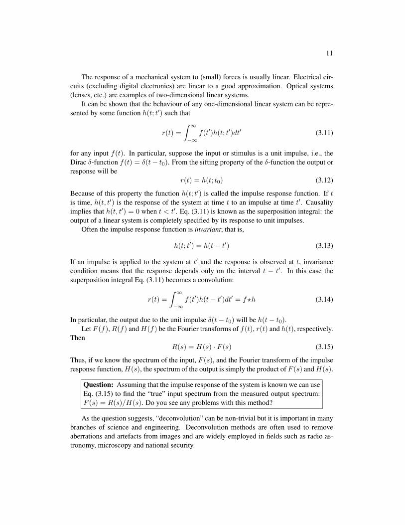
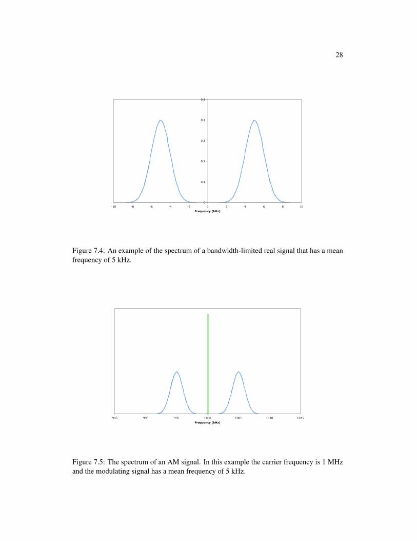
The signalm(t) is real and it follows thatM(−f) = M∗(f). To simplify the discussionassume thatm(t) is an even function. In this caseM(f) is also real and even, andM(−f) =M(f). Because it is bandwidth-limited the transform will consist of two identical “islands”located at f = ±f , where f is the instantaneous average frequency of the spectrum (seeFig. 7.4). An example of the spectrum for an AM signal is shown in Fig. (7.5). It consistsof a single narrow line at the carrier frequency f0 and two identical “sidebands” located atf0 ± f .

28

0

0.1

0.2

0.3

0.4

0.5

-10 -8 -6 -4 -2 0 2 4 6 8 10

Frequency (kHz)

Figure 7.4: An example of the spectrum of a bandwidth-limited real signal that has a meanfrequency of 5 kHz.

985 990 995 1000 1005 1010 1015

Frequency (kHz)

Figure 7.5: The spectrum of an AM signal. In this example the carrier frequency is 1 MHzand the modulating signal has a mean frequency of 5 kHz.

29

Acknowledgments

The author would like to thank the many Senior Physics staff for their feedback. I am partic-ularly grateful to Simon Fleming for his careful proofreading, Brian James for contributingthe MATLAB code in Appendix C and Mike Wheatland for suggesting a number of usefulreferences.

References

Boyd, J. P.: 2000, Chebyshev and Fourier Spectral Methods, Dover, 2nd edition

Bracewell, R. N.: 1986, The Fourier Transform and Its Application, McGraw-Hill, 2ndrevised edition

Cooley, J. W. and Tukey, J. W.: 1965, Math. Comput. 19, 297

Press, W. H., Teukolsky, S. A., T., V. W., and Flannery, B. P.: 2007, Numerical Recipes,The Art of Scientific Computing, Cambridge University Press, 3rd edition

Trefethen, L. N.: 2000, Spectral Methods in MATLAB, SIAM

30

A Some useful theorems

We collect here a number of useful theorems, some of which we have already discussed.These theorems can often be used to simplify problems. There are two groups of theorems.The first group are theorems relating functions to their Fourier transforms. The secondgroup are a collection of equalities. These most often occur in the context of time-varyngsignals, hence the use of f and t for these. Note that F (n)(s) is the nth derivative of F (s).

Theorem f(x) F(s)Similarity f(ax) |a|−1F (s/a)Addition f(x) + g(x) F (s) +G(s)Shift f(x− a) e−2πjasF (s)Modulation f(x) cos(2πfx) (1/2)F (s− f) + (1/2)F (s+ f)Convolution f(x)?g(x) F (s)G(s)Autocorrelation f(x)⊗ f(x) |F (s)|2Derivative f ′(x) 2πjsF (s)

Rayleigh∫∞−∞ f

2(t)dt =∫∞−∞ F

2(f)df

Definite integral∫∞−∞ f(t)dt = F (0)

Moment of nth order∫∞−∞ t

nf(t)dt = Fn(0)/(−2πj)n

31

B Real signals and the “analytic signal” (Advanced!!)

B.1 Definition of the analytic signal

In many discussions of Fourier transform methods one sees statements like: “For conve-nience replace cos 2πft by exp{2πjft}”. Somewhat futher along it will say: “To recoverthe real signal take the real part of the result.” See 7.1 for an example. Here we present themathematical and physical basis of this procedure.

As we have seen, the Fourier transform of a real function f(t) is Hermitian: F (−s) =F ∗(s). The negative range of the Fourier transform can thus be found by taking the com-plex conjugate of the positive range. The negative frequency range does not add any newinformation about the Fourier transform.

The presence of negative frequencies can lead to algebraic complexities and it is com-mon in signal theory, optics and other fields to introduce the analytic signal f(x) which isobtained by suppressing the negative frequency components of f(x). This analytic signal(which is not to be confused with an analytic function, which is an entirely different animal)will be complex.

Suppose we have a linear signal processing system that may correspond to a physicalprocess (for example, an imaging system using lenses, etc.) or to a digital processing al-gorithm. It is often convenient to replace the input signal by its associated analytic signal,apply the processing algorithm to this, and finally recover the real output signal. Althoughthis may seem an unnecessary complication it can greatly simplify the mathematics.

The formal—but not very practical!—definition of the analytic signal f(t) associatedwith the signal f(t) is

f(t) = f(t)− FHi(t) (B.1)

where FHi is the Hilbert transform of f(t):

FHi(t) =1

π

∫ ∞−∞

f(t′)dt′

t′ − t(B.2)

(the Cauchy principal value of the integral must be used).Bracewell gives an entirely equivalent and practical definition: for any real function

f(t) that has a Fourier transform F (s) the analytic signal corresponding to f(t) is

f(t) = 2F−1{H(s)F (s)} (B.3)

where H(s) is the Heaviside function. Operationally one takes the Fourier transform off(t), discards the negative frequency components, and then takes the inverse transform.Given the analytic signal f(t) the physical signal associated with it is

f(t) = <{f(t)} (B.4)

As an example the analytic signal corresponding to cos(t) is ejt.In the case of the DFT it is easy to show that Fk = F ∗N−k and it is possible to define an

“analytic sampled signal” analogous to the continuous analytic signal:

fn = 2N−1

[N/2]∑k=0

HkFke2πjNkn n = 0, 1, 2, . . . , N − 1 (B.5)

32

where Hk = 1 for k = 0, 1, . . . [N/2] and Hk = 0 otherwise. The notation [N/2] indicatesinteger division; e.g., [6/2] = [7/2] = 3.

The analytic signal is well suited to situations where there is a range of frequencies.Examples include the behaviour of interferometers illuminated with broadband light andthe propagation of narrow pulses along waveguides or through optical fibres.

B.2 Example: an interferometer illuminated with broadband light

-1

-0.8

-0.6

-0.4

-0.2

0

0.2

0.4

0.6

0.8

1

-10 -8 -6 -4 -2 0 2 4 6 8 10

Figure B.1: The output of an interference spectrometer illuminated with “almost”monochromatic light. The fact that the amplitude of the fringes is not constant shows thatthe light source is not monochromatic.

Fig. (B.1) shows the output from a certain interferometer illuminated by a single spectralline from an atomic vapour lamp. The fact that the amplitude of the interference signal isnot constant shows that the light source is not monochromatic.

In this example the envelope or fringe visibility can be estimated quite accurately fromthe standard Michelson formula:

V =Imax − Imin

Imax + Imin(B.6)

where Imax and Imin are successive maxima and minima of the fringe pattern. The averagewavelength can also be estimated by measuring the distance X spanned by N fringes. Theaverage wavelength is X/N .

This approach has some limitations:

• It is essentially graphical, and it is not easy to implement it in code using MATLABor a similar language.

33

-1

-0.8

-0.6

-0.4

-0.2

0

0.2

0.4

0.6

0.8

1

-10 -8 -6 -4 -2 0 2 4 6 8 10

Figure B.2: The output of an interference spectrometer illuminated with broadband light. Inthis example Michelson’s formula for finding the envelope or visibility will not be accurate.

• When the bandwidth is large it basically doesn’t work! Fig (B.2) shows an example.

The interference signal can be written as

f(x) = V (x) cos(2πνx) (B.7)

where V (x) is the envelope function (in this example, the fringe visibility) and ν is the meanfrequency.

Suppose we had a magic wand that could transform f(x) into the new function

q(x) = V (x) sin 2πνx (B.8)

This function is called the quadrature of f(x). It immediately follows from the elementaryproperties of the sine and cosine functions that

V (x) = [f2(x) + g2(x)]1/2 (B.9)

Let f(x) be the analytic signal associated with the interference signal:

f(x) = V (x)e2πjνx = V (x)[cos(2πνx) + j sin(2πνx)] = f(x) + jq(x) (B.10)

from which we see that the quadrature function is simply the imaginary part of the analyticsignal. The envelope can be found from

V (x) = |f(x)| (B.11)

34

From the shift theorem it follows that the Fourier transform of the analytic signal, F{f(x)},will be centred on the mean wavelength ν.

The same argument can be used to find the envelope function and mean frequency forsampled data using the analytic sampled signal. It is worth noting that implementing theprocedure outlined here in MATLAB or a similar language is very straightforward.

C Sample MATLAB code for calculating the FFT

The following sample code was written by Brian James. It was written specifically forExperiment 28 (Fourier Transform Spectroscopy) but can be readily adapted for other ap-plications.

The data in this case have been obtained with an interferometer (see 7.2) and havebeen saved as an ASCII text file. Each line contains an optical path difference (OPD) andintensity. The OPDs are equally spaced and there are N data points, where N is a power of2. The OPD is in nanometres, and the Fourier transform will be a function of wavenumbers,having units of nm−1. Apart from calculating the FFT (line 12) the code plots the resultsagainst wavelength and finds the wavelength and uncertainty of the the peak in the spectrum.

1. % text file is assumed to be of length 2ˆn2. FTS = load(’redLED.txt’, ’-ascii’); %loads two-column ascii file for FFT3. x = FTS(:,1); % extracts first column as linear array4. N = length(x) % number of OPD samples5. OPDs = x(2) - x(1); % OPD sampling period6. wnums = 1/OPDs; % wavenumber sampling interval7. wn = wnums/N*(0:N/2); %wavenumber array8. wl = 1./wn; %wavelength array9. y = FTS(:,2); % extracts second column as linear array10. ymean = mean(y);% mean of FTS values11. yy = y - ymean; % change men FTS to zero12. F = fft(yy); % find FFT13. Fp = F(1:N/2+1)*OPDs; %extract positive freq elements of FFT14. FFT = abs(Fp); % absolute values of FFT freq elements15. [maxspec, maxwn] = max(FFT) % find max of FFT and its wavenumber location16. wnumbermax = wn(maxwn)% wavenumber for FFT max17. wlengthmax = round(wl(maxwn)) % wavelength for FFT max, rounded to integer18. wlengthmaxerror = round(0.25*abs(wl(maxwn+1)- wl(maxwn-1))); %wavelength error19. wnplot = wn(wn>0.000833 & wn<0.00333); %select wavenumbers for 300-1200 nm20. wlplot = 1./wnplot; %convert selected wavenumbers to wavelengths21. FFTplot = FFT(wn>0.000833 & wn<0.00333);%find FFT for selected range22. plot(wlplot,FFTplot) % plot FFT for selected range23. xlabel(’Wavelength (nm)’, ’FontSize’, 14); %label x axis24. ylabel(’Intensity (a.u.)’, ’FontSize’, 14); %label y axis25. text(700,140000, [’Maximum: ’, num2str(wlengthmax), ’ +/- ’,...26. num2str(wlengthmaxerror),’ nm’], ’FontSize’,14) % print FFT max position on plot

35

�

Figure C.1: The output produced by the MATLAB code in this Appendix.