fourier approximation of symmetric ideal knots - …lcvm · july 14, 2010 10:49 wspc/instruction...

July 14, 2010 10:49 WSPC/INSTRUCTION FILE fourier

Fourier approximation of symmetric ideal knots

M. Carlen, H. Gerlach

Institut de Mathematiques B, Ecole Polytechnique Federale de Lausanne, CH-1015 Lausanne,

Switzerland, {mathias.carlen, henryk.gerlach}@epfl.ch

ABSTRACT

Enforcing a specific symmetry group on a curve, knotted or not, is not trivial usingstandard interpolations such as polygons or splines. For a prescribed symmetry groupwe present a symmetrization process based on a Fourier description of a knot. Thepresence of symmetry groups implies a characteristic pattern in the Fourier coefficients.The relations between the coefficients are shown for five ideal knot shapes with theirproposed symmetry groups.

Keywords: ideal knots, Fourier knots, symmetry of curves, Fourier coefficient pattern

Mathematics Subject Classification 2010: 49Q10, 53A04, 42B05, 58D19

1. Introduction

In the field of geometric knot theory, various discretization techniques of curves havebeen adopted. In particular, for the problem of ideal knots – minimizing the lengthof a given knot with prescribed thickness – authors have used polygons[1,17,18], arcsof circles[3], biarcs[8] and Fourier knots[16]. These representations all have their ownstrengths and limitations, such as speed of computation, complexity, convergenceor accurate approximation of curvature and torsion. Many computations suggestthat some ideal knot shapes have inherent symmetries (see Figures 2, 3, 4, 5, 6 forexamples).

In this paper we propose two results. First, a technique to exactly symmetrizean almost symmetric, closed curve, second, relationships in the pattern structure ofthe Fourier coefficients for several symmetric knots. The pattern structure can beused to reduce the number of degrees of freedom for either analytical or numericaltreatments of Fourier representations.

In the first part of the paper we briefly review the notion of ideal knots anddescribe a Fourier representation for closed curves. Then we introduce the sym-metrization process based on this parameterization. Given a symmetric knot, weshow that its Fourier coefficients are not independent and list these relationshipsfor the symmetric trefoil, figure eight knot, 51, 818 and 10123 knots. In the closingpart of the paper we discuss practical implications of these relationships to thecomputations of ideal knots.

1


2

2. Ideal Fourier knots

To a continuous closed curve γ : S −→ R3, (S = R/Z) we can assign a thickness[14]∆[γ] ∈ R, defined as the infimum of the radii of all circles passing through threepoints and corresponding to three distinct parameters, in the image of γ. Any thickcurve (i.e. ∆[γ] > 0) has a C1,1(S,R3) constant-speed parameterization[15]. For afixed knot class we call minimizers of the ropelength L[·]/∆[·] – i.e. length dividedby thickness – ideal knots.[19,14,6,13]

A periodic function f(t) can be written as a Fourier series [21,9] where thelinearly independent base functions are sin(k t) and cos(k t) for t ∈ [0, 2π) andk = 0, 1, . . .. For a closed curve γ(t), t ∈ S embedded in R3 we can therefore definethree Fourier series, one for each coordinate function of γ.

Definition 2.1. Let C be a finite sequence of pairs of R3-vectors:

C = {(ai, bi)}i=1,...,k ai, bi ∈ R3.

We can use such a sequence as Fourier coefficients and define

γ(t) :=k∑i=1

(ai cos(fit) + bi sin(fit)) , t ∈ [0, 1] (2.1)

as a curve in C∞(S,R3) with frequencies fi = 2πi. If the curve is injective, we callγ a Fourier knot[16].

Remark 2.2. Note that the sum in the above definition starts at i = 1 and theconstant a0 is neglected. This term is independent of the parameter t and thereforejust a translation of the Fourier knot.

The Fourier representation of knots has been used in [16,22], where the emphasisis on finding simple Fourier shapes of given knot types. The following lemma justifiesthe use of Fourier knots to approximate ideal knot shapes.

Lemma 2.3. Let γ ∈ C1,1(S) be an ideal shape. Then for every ε > 0 there existsa finite set of coefficients {(ai, bi)}i such that the Fourier knot

γε(t) :=∑i

(ai cos(fit) + bi sin(fit))

satisfies

‖γ − γε‖C1(S) < ε and ∆[γ]− ε < ∆[γε].

Proof. By [11, Corollary 3.3] there exists a curve γ∞,ε ∈ C∞(S,R3) such that

‖γ − γ∞,ε‖C1(S,R3) < ε/2 and ∆[γ]− ε/2 < ∆[γ∞,ε].

By standard Fourier theory there exists a sequence {γi}i of Fourier curves – eachrepresented by a finite number of coefficients – that approximate γ∞,ε in a C2-fashion. This approximation satisfies the hypotheses of [11, Lemma 3.2] and for a


3

large enough index i∗ we have

‖γ∞,ε − γi∗‖C1(S) < ε/2, ∆[γ∞,ε]− ε/2 < ∆[γi∗ ].

Now γε := γi∗ is the sought Fourier knot. Ideality of γ and C1-convergence implythat indeed L[γε]

∆[γε] →L[γ]∆[γ] for ε→ 0.

3. Symmetry of curves

The definitions we give hereafter stress that a curve has a symmetry if and only ifthe resulting shape is identical to the original with respect to its parameterization.In other words, let γ be the original curve and γsym the shape after a symmetry hasbeen applied. It is in fact only a symmetry if γ(s) = γsym(s) for all s (see Example3.5).

Definition 3.1. Let γ : S −→ RN be a curve and G ⊂ Aut(C0(S,RN )) a groupacting on C0(S,RN ). We call γ G-symmetric if

gγ = γ ∀g ∈ G.

We then call G a symmetry-group of γ.

Here Aut is the automorphism group, which is the set of bijective mappingsfrom a mathematical object to itself. If G is maximal in some respect, we may call it‘the’ symmetry-group of γ. Just taking the maximal subgroup G of Aut(C0(S,R3))such that γ is G symmetric is not what we want since it is too large. For example itwould include all H defined for each homeomorphism h : R3 −→ R3 with h ◦ γ = γ

as H[α] := h ◦ α for α ∈ C0(S,R3).Now we can state how to actually symmetrize a given closed curve (see Figure 7).

Definition 3.2. Let γ ∈ C0(S,R3) be some curve and G ⊂ Aut(C0(S,R3)) a finitegroup. Then we call

γG :=

∑g∈G gγ

|G|the G-symmetrization of γ.

As mentioned above, the parameterization of a knot plays an important rolewhen dealing with symmetries. We now provide the tools needed to ensure that acurve and its symmetry image are identical.

Definition 3.3. For x ∈ R we define the parameter shift σx : C0(S,R3) −→C0(S,R3) by x of a curve γ ∈ C0(S,R3) as

σx[γ](t) := γ(t+ x)

and the parameter reflection %x : C0(S,R3) −→ C0(S,R3) around x as

%x[γ](t) := γ(2x− t).


4

Lemma 3.4. Shifts and reflections form a group

P := {σx : x ∈ R} ∪ {%y : y ∈ R} ⊂ Aut(C0(S,RN ))

and for x, y ∈ R

(i) σx ◦ σy = σx+y,(ii) %y ◦ %x = σy−x,

(iii) %x ◦ σy = %x−y/2 = σ−y ◦ %x.

2

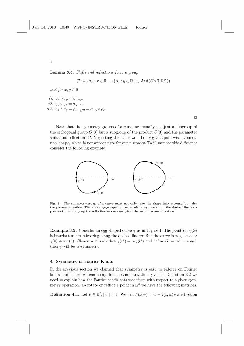
Note that the symmetry-groups of a curve are usually not just a subgroup ofthe orthogonal group O(3) but a subgroup of the product O(3) and the parametershifts and reflections P. Neglecting the latter would only give a pointwise symmet-rical shape, which is not appropriate for our purposes. To illuminate this differenceconsider the following example.

γ(t∗)

γ(0)

m

mγ(0)

mmγ(t∗)

Fig. 1. The symmetry-group of a curve must not only take the shape into account, but alsothe parameterization: The above egg-shaped curve is mirror symmetric to the dashed line as apoint-set, but applying the reflection m does not yield the same parameterization.

Example 3.5. Consider an egg shaped curve γ as in Figure 1. The point-set γ(S)is invariant under mirroring along the dashed line m. But the curve is not, becauseγ(0) 6= mγ(0). Choose a t∗ such that γ(t∗) = mγ(t∗) and define G := {id,m ◦ %t∗}then γ will be G-symmetric.

4. Symmetry of Fourier Knots

In the previous section we claimed that symmetry is easy to enforce on Fourierknots, but before we can compute the symmetrization given in Definition 3.2 weneed to explain how the Fourier coefficients transform with respect to a given sym-metry operation. To rotate or reflect a point in R3 we have the following matrices.

Definition 4.1. Let v ∈ R3, ||v|| = 1. We call Mv(w) = w − 2〈v, w〉v a reflection


5

along v. The linear map Mv mirrors on the hyperplane orthogonal to v. We call

Dv,α =

cosα+ v21 (1− cosα) v1v2 (1− cosα)− v3 sinα v1v3 (1− cosα) + v2 sinα

v2v1 (1− cosα) + v3 sinα cosα+ v22 (1− cosα) v2v3 (1− cosα)− v1 sinα

v3v1 (1− cosα)− v2 sinα v3v2 (1− cosα) + v1 sinα cosα+ v23 (1− cosα)

a rotation around v by α ∈ R.

The next lemma describes how the coefficients in the Fourier representationtransform when we reflect or rotate a Fourier knot or shift its parameterization.

Lemma 4.2. Let γ(t) =∑i (ai cos(fit) + bi sin(fit)) be a Fourier knot.

• Let M ∈ O(3) be an orthogonal matrix. Then

(Mγ)(t) =∑i

(ai cos(fit) + bi sin(fit)

)with

ai = Mai, bi = Mbi,

or block-wise (aibi

)= U

(aibi

), where U =

(M 00 M

).

• Let σx be a parameter shift by some x ∈ R. Then

(σxγ)(t) =∑i


)with

ai = cos(fix)ai + sin(fix)bi, bi = − sin(fix)ai + cos(fix)bi,

or block-wise(aibi

)= Sx

(aibi

), where Sx =

(cos(fix)I sin(fix)I− sin(fix)I cos(fix)I

).

• Let %x be a parameter reflection around x ∈ R. Then

(%xγ)(t) =∑i


)with

ai = cos(2fix)ai + sin(2fix)bi, bi = sin(2fix)ai − cos(2fix)bi,

or block-wise(aibi

)= Rx

(aibi

), where Rx =

(cos(2fix)I sin(2fix)Isin(2fix)I − cos(2fix)I

).

• A composition g of orthogonal maps, parameter shifts and reflections acts onthe Fourier coefficients of frequency fi by a matrix Fg,i that is a product of thecorresponding block matrices U, Sx and Rx above.


6

2

Note that matrices Sx and Rx corresponding to the parameter shifts and reflectionscommute with the orthogonal matrices U as expected.

A priori we do not know a symmetry group for an ideal knot since there is noanalytic expression for most of them. However studying approximately ideal shapesobtained by the numerical computations suggests possible symmetries.

Conjecture 4.1. After a reparametrization, a translation and a rotationthe following symmetry-groups are suggested by the numerical data :

• Trefoil (31) [1,4,8,20]:

G31 = {(D(0 0 1)t,2π/3 ◦ σ1/3)i ◦ (D(1 0 0)t,π ◦ %0)j : i = 0, 1, 2, j = 0, 1}.

This group has six elements and is isomorphic to the symmetric groupof degree 3.

• Figure eight knot (41) [1,8,20]:

G41 = {(D(0 1 0)t,π ◦ σ1/2)i ◦ (M(0 1 0)t ◦D(0 1 0)t,π/2 ◦ σ1/4)j : i, j = 0, 1}.

This group has |G41 | = 4 elements.• The 51-knot[1] has only two elements in its symmetry group given by

G51 = {(D(0 1 0)t,π ◦ %0)j : j = 0, 1}.

• The 818-knot[1] appears to be highly symmetric with 32 elements inits symmetry group given by

G818 = { (D(0 0 1)t,π/2 ◦ σ−1/4)i ◦ (M(0 0 1)t ◦D(0 0 1)t,π/4 ◦ σ5/8)j

: i = 0, . . . , 3, j = 0, . . . , 7}.

• The 10123-knot[1] also appears to be highly symmetric with 50 elementsin its symmetry group :

G10123 = { (D(0 0 1)t,2π/5 ◦ σ−3/5)i ◦ (M(0 0 1)t ◦D(0 0 1)t,π/5 ◦ σ−3/10)j

: i = 0, . . . , 4, j = 0, . . . , 9}.

The symmetries for these knots are visualized in Figures 2, 3, 4, 5 and 6. Thetrefoil has a 3-symmetry by rotating the knot by an angle of 2π/3 around a firstsymmetry axis. The second set of symmetries is a rotation by π around the axisfrom the center of the knot through the middle of an ear as seen in Figure 2. Thegenerators of the symmetry group are one of each type stated before. Figure 7illustrates the symmetrization process on a perturbed trefoil knot γ31 , the 6 inter-mediate shapes gγ31 for g ∈ G31 and the final symmetrized trefoil knot. The figureeight knot has a slightly less obvious symmetry group. A rotation by π about thesymmetry axis in Figure 3 is a first symmetry. Another symmetry is obtained byrotating the knot by π/2 around the same axis and reflecting it through the trans-parent plane. Together they generate a symmetry group with four elements. Finally


7

the 51-knot can be mapped to itself by a rotation by π around the only symmetryaxis as depicted in Figure 4. The authors in [1] briefly discuss the symmetries forthe 818 and 10123 knots. They do not explicitly state the symmetries which arefirst, a rotation by π/2 (2π/5 for the 10123) around the central symmetry axis andsecond, a rotation by π/8 (π/10 for the 10123) followed by a reflection on the planeorthogonal to the symmetry axis. Note that we did not include the reparametriza-tion in our explanation since it is intrinsic to the curve and not visualized in thefigures.

Theorem 4.3. Let γ(t) =∑ki=1 (ai cos(fit) + bi sin(fit)) , t ∈ [0, 1] be a curve in

C∞(S,R3) with coefficients ai, bi ∈ R3, frequencies fi = 2πi and let G be a finitesubgroup of actions such that each action g can be represented for each frequencyfi by a block-matrix Fg,i as in Lemma 4.2. Then γ is G-symmetric iff(

aibi

)= Fi

(aibi

)for all i = 1, . . . , k (4.1)

where

Fi :=

∑g∈G Fg,i

|G|∈ R6×6 (4.2)

is the frequency-wise average.

Proof. First, we note that two Fourier knots describe the same curve iff all coef-ficients coincide, since sin(fit) and cos(fit) form an orthogonal basis. Second, wenote that some curve γ is G-symmetric iff γ = γG pointwise. Consequently, we have(

aibi

)= Fi

(aibi

)(4.3)

for each frequency fi iff γ is G symmetric as claimed.

Lemma 4.4. Let G = {g1, . . . , gn} be a finite subgroup of R3×3 × P.

(i) Then each element gj ∈ G can be represented either as gj = αj ◦ σpjor

gj = αj ◦ %qj with αj ∈ R3×3 and pj ∈ Q, qj ∈ R.(ii) If all parameter reflections occur around rational parameters, i.e. qj ∈ Q as in

(i) for all j, then there exists some k ∈ N such that kqj and kpj are integersfor all j and

Fi :=

∑g∈G Fg,i

|G|= Fi+k for all i ∈ N.

Proof.

(i) The representation is a direct consequence of Lemma 3.4. It remains to showthat pj is rational. Assume pj was irrational. Then {gij : i ∈ N} ⊂ G would beinfinite contradicting the finiteness of G.


8

(ii) Since pj and qj are rational, define k as the least common multiple of all denom-inators. Then kqj and kpj are integers. Consequently in Lemma 4.2 we havecos(fipj) = cos(2πipj) = cos(2πix + 2πkpj) = cos(2π(i + k)x) = cos(fi+kx)and likewise sin(fipj) = sin(fi+kpj) which implies Fi = Fi+k.

Remark 4.5. If a curve γ is G-symmetric and Fi are the frequency-wise averagesthen σxγ is σxGσ−x-symmetric and the identity (4.3) becomes(

aibi

)= SxFiS−x

(aibi

).

In particular the identity remains unchanged if G does not contain parameter re-flections. Similarly the coefficients of %xγ satisfy(

aibi

)= RxFiRx

(aibi

).

As suggested in Conjecture 4.1, the trefoil knot, the figure eight, the 51, 818

and the 10123 are believed to have particular symmetry groups. We now derive thecoefficient relations for these knots using equation 4.1 and the different matricesintroduced in Lemma 4.2.

Example 4.6. Assume that symmetry Conjecture 4.1 is true. Then the Fouriercoefficients must fulfill the following equations:

(i) Trefoil: Computing (4.2) yields :

F3i+1 =

1/2 0 0 0 −1/2 00 0 0 0 0 00 0 0 0 0 00 0 0 0 0 0

−1/2 0 0 0 1/2 00 0 0 0 0 0

, F3i+2 =

1/2 0 0 0 1/2 00 0 0 0 0 00 0 0 0 0 00 0 0 0 0 0

1/2 0 0 0 1/2 00 0 0 0 0 0

, F3i+3 =

0 0 0 0 0 00 0 0 0 0 00 0 0 0 0 00 0 0 0 0 00 0 0 0 0 00 0 0 0 0 1

,

for i ∈ N and by Lemma 4.4 it is enough to compute the first three matrices.By Theorem 4.3 we deduce that the only non-zero coefficients are :

a3i+1,1 = −b3i+1,2, a3i+2,1 = b3i+2,2, b3i+3,3,

with the notation af,k, where f is the frequency and k the coordinate index.These conventions will also be used for the following knots. For the trefoil, thismeans that there are 3 independent, non-zero coefficients out of 18.

(ii) 41: For i ∈ N:

a4i+1,1 = b4i+1,3, a4i+1,3 = −b4i+1,1,

a4i+2,2, b4i+2,2,

a4i+3,1 = −b4i+3,3, a4i+3,3 = b4i+3,1,

with 6 independent coefficients out of 24.(iii) 51: For i ∈ N:

ai,2, bi,1, bi,3,

with 3 independent coefficients out of 6.


9

(iv) 818: For i ∈ N :

a8i+3,1 = b8i+3,2, a8i+3,2 = −b8i+3,1,

a8i+4,3, b8i+4,3,

a8i+5,1 = −b8i+5,2, a8i+5,2 = b8i+5,1,

with 6 independent coefficients out of 48.(v) 10123: For i ∈ N :

a10i+3,1 = −b10i+3,2, a10i+3,2 = b10i+3,1,

a10i+5,3, b10i+5,3,

a10i+7,1 = b10i+7,2, a10i+7,2 = −b10i+7,1,

with 6 independent coefficients out of 60.

5. Conclusion

We saw in Lemma 2.3 that ideal knots can be approximated by Fourier knots merelyas a consequence of standard Fourier approximation theory. We then presented aprocedure to symmetrize approximately symmetric ideal knot shapes for a Fourierrepresentation. Specifically, for a curve with a certain symmetry group, we havederived a way to compute the characteristic pattern in the Fourier coefficients dueto the symmetries (Lemma 4.6). In practice, the original shape used in the sym-metrization process has to be close to ideal and close to the enforced symmetries,otherwise the resulting knot might not even be in the same isotopy class. A circlefor example is an ideal shape, has all the above symmetries, and its Fourier coeffi-cients do fulfill the relations in Lemma 4.6, however it is none of the knot types wediscussed.

In Example 4.6 we have seen that symmetries of a curve imply identities of itsFourier coefficients. This could, for example, be used as a measure of how symmetrica curve is. More important, the converse is also true: if we enforce the identities,then we enforce the symmetry on the Fourier knot and at the same time reduce thedegrees of freedom. For example only one sixth of the Fourier trefoil (31) coefficientsare non-zero compared to the original shape without enforcing the symmetry. Weused this to speed up the approximation of an ideal trefoil[7,10], improving thenaturally slow simulated annealing algorithm[8].

6. Acknowledgements

Research supported by the Swiss National Science Foundation SNSF No. 117898and SNSF No. 116740. We would like to thank Professors Eric Rawdon and JohnH. Maddocks for interesting discussions and helpful comments.


10

References

[1] Ashton, T.; Cantarella, J.; Piatek, M.; Rawdon, E. Knot Tightening By ConstrainedGradient Descent. arXiv:1002.1723v1 [math.DG], (2010).

[2] Ashton, T.; Cantarella, J.; Piatek, M.; Rawdon, E. Self-contact sets for 50 tightlyknotted and linked tubes. math.DG/0508248 in prepation, (2005).

[3] J. Baranska, P. Pieranski, and E.J. Rawdon, Ropelength of tight polygonal knots, in[5], 293–321.

[4] J. Baranska, S. Przybyl, and P. Pieranski, Curvature and torsion of the tight closedtrefoil knot, Eur. Phys. J. B 66, 547–556 (2008).

[5] J.A. Calvo, K.C. Millett, E.J. Rawdon, A. Stasiak (eds.) Physical and NumericalModels in Knot Theory, Ser. on Knots and Everything 36, World Scientific, Singapore(2005).

[6] Cantarella, J.; Kusner, R.B.; Sullivan, J.M. On the minimum ropelength of knotsand links. Inv. math. 150 (2002), 257–286.

[7] Carlen, M. Computation and visualization of ideal knot shapes, PhD thesis No. 4621,EPF Lausanne (2010),http://library.epfl.ch/theses/?display=detail&nr=4621.

[8] Carlen, M.; Laurie, B.; Maddocks, J.H.; Smutny, J. Biarcs, Global Radius of Curva-ture, and the Computation of Ideal Knot Shapes in [5], 75–108.

[9] Folland, G. B., Fourier Analysis and Its Applications, Brooks/Cole Publishing Co.(1992).

[10] Gerlach, H. Ideal Knots and Other Packing Problems of Tubes, PhD thesis No. 4601,EPF Lausanne (2010),http://library.epfl.ch/theses/?display=detail&nr=4601.

[11] Gerlach, H.; von der Mosel, H. What are the longest ropes on the unit sphere? ReportNr. 32, Institut fur Mathematik, RWTH Aachen (2009).

[12] Gilbert, B. Ideal knot and link data. Accessed 3rd March 2010.http:

//katlas.math.toronto.edu/w/index.php?title=Ideal_knots&oldid=1692192

[13] Gonzalez, O.; de la Llave, R. Existence of Ideal Knots, Journal of Knot Theory andIts Ramifications 12, No. 1 (2003) 123–133.

[14] Gonzalez, O.; Maddocks, J.H. Global Curvature, Thickness and the Ideal Shapes ofKnots, Proc. Natl. Acad. Sci. USA 96 (1999), 4769–4773.

[15] Gonzalez, O.; Maddocks, J.H.; Schuricht, F.; von der Mosel, H. Global curvature andself-contact of nonlinearly elastic curves and rods, Calc. Var. 14 (2002), 29–68.

[16] Kauffman, L.H. Fourier Knots, in [19], 364–373.[17] Laurie B., Annealing Ideal Knots and Links: Methods and Pitfalls, in [19], 42–51.[18] Pieranski P., In Search of Ideal Knots, in [19], 20–41.[19] A. Stasiak, V. Katritch, L.H. Kauffman (Eds.), Ideal Knots, Series on Knots and

Everything Vol. 19, World Scientific, Singapore (1998).[20] Smutny, J. Global radii of curvature and the biarc approximation of spaces curves:

In pursuit of ideal knot shapes, PhD thesis No. 2981, EPF Lausanne (2004),http://library.epfl.ch/theses/?display=detail&nr=2981.

[21] Stein, E. M. and Weiss, G., Introduction to Fourier Analysis on Euclidean Spaces,Princeton University Press, (1971).

[22] Trautwein, A.K. An introduction to harmonic knots, in [19], 353–363.

http://library.epfl.ch/theses/?display=detail&nr=4621


http://katlas.math.toronto.edu/w/index.php?title=Ideal_knots&oldid=1692192

http://katlas.math.toronto.edu/w/index.php?title=Ideal_knots&oldid=1692192



11

Fig. 2. Trefoil symmetry axes for two different views. The axis with the prism on top is the 3-symmetry with rotation angles of 2π/3. The three ellipsoid ended axis give the second symmetry,which is a rotation of angle π. The generators of the symmetry group are one element of bothtypes[4].

Fig. 3. Three different views of the figure-eight knot symmetries. The first symmetry is a rotationof angle π around the symmetry axis visualized in the image. The second generator of the symmetrygroup is a reflection through the plane and then a rotation of angle π/2 around the symmetryaxis.

Fig. 4. The symmetry group for the 51 knot has only a single generator, which is a rotation ofangle π about the symmetry axis shown in the image.


12

Fig. 5. The symmetries of the 818 are generated by a π/2 rotation and the composition of areflection and a π/4 rotation.

Fig. 6. The symmetries of the 10123 are generated by a 2π/5 rotation and the composition of areflection and a π/5 rotation..

Fig. 7. The symmetrization process of Definition 3.2 visualized. Starting from a not completelysymmetric trefoil in the left corner, we apply each element of the presumed symmetry group to itand take the average to receive a symmetric shape in the lower right corner.

fourier approximation of symmetric ideal knots - …lcvm · july 14, 2010 10:49 wspc/instruction...

Documents