fourier analysis on the lorentz group and relativistic quantum mechanics
TRANSCRIPT

FOURIER ANALYSIS ON THE LORENTZ GROUPAND RELATIVISTIC QUANTUM MECHANICS
A Thesis Submitted tothe Graduate School of Engineering and Sciences of
Izmir Institute of Technologyin Partial Fulfillment of the Requirements for the Degree of
MASTER OF SCIENCE
in Mathematics
byZahide OK
June 2008IZMIR

We approve the thesis of Zahide OK
Prof. Dr. Rıfat MIRKASIMSupervisor
Prof. Dr. Recai ERDEMCommittee Member
Assoc. Prof. Dr. Gamze TANOGLUCommittee Member
19 June 2008Date
Prof. Dr.Oguz YILMAZ Prof. Dr. M. Hasan BOKEHead of the Mathematics Department Dean of the Graduate School of
Engineering and Sciences

ACKNOWLEDGEMENTS
I would like to thank my advisor Prof. Dr. Rıfat Mirkasım for his continual advice,
supervision and understanding in research and writing of this thesis. I would also like to
thank my family; Ok, Ozsan, Aktas and Tuna Bayrakdar for their love and infinite moral
support.
ABSTRACT
FOURIER ANALYSIS ON THE LORENTZ GROUP AND
RELATIVISTIC QUANTUM MECHANICS
The non-relativistic Schrodinger and Lippman-Schwinger equations are de-
scribed. The expressions of these equations are investigated in momentum and configura-
tion spaces, using Fourier transformation. The plane wave, which is generating function
for the matrix elements of three dimensional Euclidean group in spherical basis, expanded
in terms of Legendre polynomials and spherical Bessel functions. Also explicit calcula-
tion of Green’s function is done.
The matrix elements of the unitary irreducible representations of Lorentz group
are used to introduce Fourier expansion of plane waves. And the kernel of Gelfand-
Graev transformation, which is the relativistic plane wave, is expanded in to these matrix
elements. Then relativistic differential difference equation in configuration space is con-
structed.
Lippman-Schwinger equations are studied in Lobachevsky space (hyperbolic
space). An analogous to the non-relativistic case, using the finite difference Schrodinger
equation, one dimensional Green’s function is analyzed for the relativistic case . Also the
finite difference analogue of the Heavyside step function is investigated.
iv
OZET
LORENTZ GRUBU UZERINE FOURIER ANALIZI VE
ROLATIVISTIK KUANTUM MEKANIGI
Rolativistik olmayan Schrodinger ve Lippman-Schwinger denklemleri
tanımlandı. Bu denklemlerin hem momentum hem de konfigurasyon uzayındaki
ifadeleri Fourier donusumu kullanılarak incelendi. Uc boyutlu Oklid grubunun kuresel
bazlarca ifade edilen matris elemanlarının doguranı olan ”duzlem dalga” nın seri acılımı,
Legendre polinomları ve kuresel Bessel fonksiyonları cinsinden yapıldı. Bunun yanısıra,
dalga denkleminde kullanılmak uzere, Green fonksiyonunun hesabı gerceklestirildi.
Lorentz grubunun birimsel indirgenemez temsillerinin matris elemanları tanıtıldı
ve bu elemanlar kullanılarak Gelfand-Graev donusumlerinin cekirdegi olan rolativistik
dalga fonksiyonunun seri acılımı gerceklestirildi. Bu bakıs acısıyla, konfigurasyon
uzayında, sonlu fark Schrodinger denklemi yapılandırıldı.
Rolativistik olmayan denklemlerin benzeri olan rolativistik Lippman-Schwinger
denklemlerini yapılandırmak uzere uc boyutlu Lobachevsky uzayında calısıldı. Son
olarak, sonlu fark Schrodinger denklemi kullanılarak, rolativistik dalga denkleminde kul-
lanılmak uzere, bir boyutlu Green fonksiyonun hesabı gerceklestirildi.
v
TABLE OF CONTENTS
CHAPTER 1 . INTRODUCTION . . . . . . . . . . . . . . . . . . . . . . . . . viii
CHAPTER 2 . A BRIEF REVIEW OF NON-RELATIVISTIC
SCATTERING THEORY . . . . . . . . . . . . . . . . . . . . . 1
2.1. Non-Relativistic Two Body Problem . . . . . . . . . . . . . . 1
2.2. General Formalism of Non-Relativistic Scattering Theory . . 3
2.3. Partial Wave Analysis . . . . . . . . . . . . . . . . . . . . . . 6
2.3.1. The plane wave expansion and related relations . . . . . . 6
2.3.2. Wave function expansion . . . . . . . . . . . . . . . . . . 9
CHAPTER 3 . RELATIVISTIC Q.M. BASED ON THE CONCEPT OF THE
RELATIVISTIC CONFIGURATION SPACE . . . . . . . . . . . 15
3.1. Lorentz Group Representations and Relativistic Position
Operator . . . . . . . . . . . . . . . . . . . . . . . . . . . . . 15
3.2. Relativistic Plane Wave Partial Expansion . . . . . . . . . . . 18
3.3. Relativistic Differential Difference Schrodinger Equation . . . 21
CHAPTER 4 . RELATIVISTIC TWO-BODY PROBLEM AND
RELATIVISTIC SCATTERING THEORY . . . . . . . . . . . . 30
4.1. General Theory . . . . . . . . . . . . . . . . . . . . . . . . . 30
4.2. Evaluation of Green Function . . . . . . . . . . . . . . . . . 35
4.3. Finite Difference Analogue of the Heavyside Step Function
and Bernoulli Numbers . . . . . . . . . . . . . . . . . . . . . 39
4.4. Scattering Theory . . . . . . . . . . . . . . . . . . . . . . . . 42
4.5. The Jost Functions . . . . . . . . . . . . . . . . . . . . . . . 45
CHAPTER 5 . CONCLUSION . . . . . . . . . . . . . . . . . . . . . . . . . . 47
REFERENCES . . . . . . . . . . . . . . . . . . . . . . . . . . . . . . . . . . . 50
APPENDICES . . . . . . . . . . . . . . . . . . . . . . . . . . . . . . . . . . . 51
vi

APPENDIX A. BESSEL FUNCTIONS . . . . . . . . . . . . . . . . . . . . . . 51
A.1. Bessel Differential Equation . . . . . . . . . . . . . . . . . . 51
A.2. Spherical Bessel Functions . . . . . . . . . . . . . . . . . . . 52
A.3. A Fundamental System of Solutions of Bessel’s Equation . . 52
APPENDIX B. LEGENDRE FUNCTIONS . . . . . . . . . . . . . . . . . . . . 54
B.1. Legendre Differential Equation . . . . . . . . . . . . . . . . . 54
B.2. Rodrigues’ Formula . . . . . . . . . . . . . . . . . . . . . . . 55
APPENDIX C. LORENTZ GROUP . . . . . . . . . . . . . . . . . . . . . . . . 56
APPENDIX D. GROUP REPRESENTATIONS . . . . . . . . . . . . . . . . . . 58
vii

CHAPTER 1
INTRODUCTION
The description of the two-particle relativistic system is one of the central prob-
lems of the Quantum Field Theory. Traditionally for studying this problem in the frame-
work of the four-dimensional Feynman-Dyson’s formalism the covariant equation was
used known under the name ”Bethe and Salpeter equation”. This equation being advan-
tageous in many senses is nevertheless not completely satisfactory. In particular, in the
4-dimenional Bethe-Salpeter approach the clear treatment of the wave function depen-
dence of the relative time of two particles is absent.( Salpeter, et al. 1951, Landau and
Lifshitz 1958, Davydov 1963, Kadyshevsky, et al. 1968, Kadyshevsky 1988, Kagra-
manov, et al. 1989, Mir-Kasimov , et al. 1990, Mir-Kasimov 1991, Thaller 1992,
Nagiev 1995, Mir-Kasimov 2000, Mir-Kasimov 2002, Mir-Kasimov, et al. 2003)
The natural question arises: does in the framework of the covariant field theory
such formalism exist, which is from the one hand side three dimensional and admits the
probabilistic interpretation of the wave function and from the other hand side possesses
all main advantages (renormalisibility, analyticity) of the completely covariant approach.
There exist several formulations (unified under common title ”quasi-potential approach”)
of the 3-dimensional relativistic 2-body problem which give a positive answer to this
question. In the momentum representation the equations of quasi-potential approach are
the direct relativistic generalizations of the standard (non-relativistic) Schrodinger and
Lippmann-Schwinger equations. The goal of this Thesis is to consider and apply to
solution of scattering theory the concept of the relativistic configurational space in the
framework of the quasi-potential approach.
The concept of relativistic configurational space is based on the simple observation
that a free motion of a relativistic particle can be described on the basis of the Gelfand-
Graev transformation , i.e., expansion in relativistic spherical functions. ( Kontorovich
and Lebedev 1938, Bateman 1953, Gel’fand, et al. 1966, Vilenkin 1968, Biedenharn
1989). We start with the well-known fact that the equation describing the relativistic
relation between energy and momentum of the particle ( mass shell equation), describes
at the same time the three-dimensional momentum space of constant negative curvature
viii

or the Lobachevsky space. The isometry group of this space is the Lorentz group. To
introduce an adequate Fourier expansion, we must find the matrix elements of the unitary
irreducible representations of this group. These matrix elements are the eigen-functions
of the Casimir operator, or the Laplace-Beltrami operator in the Lobachevsky space
Later on it became clear that the geometry of relativistic configurational space
carries the non-commutative geometry (its ”Snyder version”). ( Carlitz 1957, Witten
1986, Deser, et al. 1988 , Witten 1988, Kadyshevsky and Fursaev 1990, Wess and
Zumino 1990, Dubois-Violette, et al.1990, Mir-Kasimov 1991, Connes 1994, Madore
1995, Dimakis and Muller 1998, Mir-Kasimov 2000, Guven, et al. 2001).
It is important to stress also the connection of given approach with q-deformations.
( Kulish 1981, Manin 1988, Woronowich 1989, Kulish 1991, Floreanini, et al. 1991,
Mir-Kasimov 1996). The oscillator model in relativistic configurational space is an ex-
plicit realization of the q-oscillator. ( Macfarlane 1989, Mir-Kasimov 1991, Rajagopal
1993).
C =1
2MµνMµν µ, ν = 0, 1, 2, 3 (1.1)
Eigenfunctions of C are unitary irreducible representations of the Lorentz group and can
be written in a form of the Gelfand - Graev kernels
< r | p >=
(p0 − p · n
mc
)−1−i rλ
(1.2)
r = rn n2 = 1 0 ≤ r <∞ (1.3)
λ =~mc
Compton wave length of the particle (1.4)
Note that r in (1.3) does not transform as the spatial component of a four vector.
There are several strong arguments for considering r as a relativistic position vec-
tor of the particle:
1. The range of variation of r (1.3) coincides with that of the standard non-relativistic
coordinate vector.
2. The magnitude r of r is Lorentz invariant in full analogy with the non-relativistic
relative distance, which is Galilean invariant.
ix

3. ”Relativistic plane wave” < r | p > in the non-relativistic limit
|p| mc r λ p0 ' mc+p2
2mc(1.5)
goes over into the standard non-relativistic plane wave
< r | p >' exp(irp·n
~
)= exp
(ip·x~
)(1.6)
In the last expression x denotes the standard non-relativistic position vector.
4. The most important physical argument is that there exists in r-space the differential
– difference operator H0 of free energy
H0 = mc2cosh iλ∂
∂r+ i
λ
rsinh iλ
∂
∂r− λ2
r2∆ϑ,φ e
λ ∂∂r (1.7)
such that
(H0 − E
)< r | p >= 0 (1.8)
The last two equations show that the plane wave < r | p > is the wave function of
the relativistic free particle, i.e. the state with a fixed value of the relativistic energy
and momentum. It is worthwhile to stress that (1.8) can be considered as a solution
of the problem of extracting the square root in the expression for the relativistic
energy
E =p0
c=√
p2c2 +m2c4 (1.9)
in a form of differential – difference operator (1.7)
The ”price” for this extraction is the presence of the exponential derivation which
amounts to a finite-difference character of the Hamiltonian operator (1.7). The interac-
tion can be described in terms of a potential function V (r). On this basis, the quantum
theory in the relativistic configurational space had been developed. This theory will be
called hereafter the Relativistic Quantum Mechanics (RQM). It proved to be an efficient
approach to solving problems in a wide range: from analytic properties of relativistic
x

wave functions and amplitudes to relativistic confinement models of composite hadrons.
We refer the reader further references therein where this theory is presented.
In chapter two the non-relativistic Schrondinger and Lippman-Schwinger equa-
tions are described in both momentum and configuration spaces, using Fourier transfor-
mation. The plane wave expansion and it’s group theoretical meaning is described.
In chapter three the matrix elements of the unitary irreducible representations of
Lorentz group are used to introduce Fourier expansion of plane waves. Then relativistic
differential difference equation in configuration space is constructed.
Finally in chapter four relativistic two-body problem and general formalism of the
scattering theory and related equations are described. Lippman-Schwinger equations are
described in Lobachevsky (hyperbolic)space.
xi

CHAPTER 2
A BRIEF REVIEW OF NON-RELATIVISTIC
SCATTERING THEORY
2.1. Non-Relativistic Two Body Problem
This chapter in a sense is introductory. We analyze here the non-relativistic two-
body problem giving the group-theoretical interpretation of a number of aspects of this
well established theory keeping in mind to generalize these properties if possible from the
non-relativistic (Galilean) case to the relativistic (Lorentz) case.
It is well known from classical mechanics that in the non-relativistic theory, the
problem of the scattering of a particle of mass m1 by a particle of mass m2, when the
interaction V (r) between the particles depends on the relative coordinate, amounts to a
problem of the scattering of a single effective particle with reduced mass in a potential
field V (r). This reduction of the problem of the elastic scattering of two particles to the
motion of a fictitious particle with reduced massm in the potential field V (r) is realized by
the simple change to a system of coordinates fixed in the center of mass of the colliding
particles,( Davydov 1963). Now let us show this reduction. The Hamiltonian of two
particles with masses m1 and m2 for the stationary state has the form;
H =p2
1
2m1
+p2
2
2m2
+ V (r1, r2) (2.1)
We introduce new variables; the center of mass radius vector R and the relative position
vector r defined by
R =m1r1 +m2r2
M, r = r1 − r2 (2.2)
where M = m1 +m2 is total mass and
P = p1 + p1, p =m2p1 −m1p2
m1 +m2
(2.3)
P and p are total and relative momenta respectively.
Now considering the relation
−i~ ∂
∂ri
= pi (i = 1, 2) (2.4)
1
we can determine the equation which describes the motion of the center of mass. Let’s
write r1 and r2 as;
r1 =m2
Mr + R
r2 = −m1
Mr + R (2.5)
and determine the following
∂
∂r1
=∂R∂r1
∂
∂R+
∂r∂r1
∂
∂r=m1
M
∂
∂R+
∂
∂r∂
∂r2
=∂R∂r2
∂
∂R+
∂r∂r2
∂
∂r=m2
M
∂
∂R− ∂
∂r. (2.6)
Now we insert these relations into Hamiltonian equation;
H = − ~2
2m1
(m1
M
∂
∂R+
∂
∂r
)2
− ~2
2m2
(m2
M
∂
∂R− ∂
∂r
)2
+ V (R, r) (2.7)
= − ~2
2M
(∂
∂R
)2
− ~2
2
(1
m1
+1
m2
)(∂
∂r
)2
+ V (R, r) (2.8)
and substitute1
m1
+1
m2
=m1 +m2
m1m2
=1
m, m =
m1m2
M(2.9)
where m is the reduced mass and M is the total mass of the system. Then equation (2.8)
can be written in the form
H = − ~2
2M∇2
R −~2
2m∇2
r + V (R, r) (2.10)
=P2
2M+
p2
2m+ V (R, r) (2.11)
= Hcm + H (2.12)
This equation represents the separation of H into the Hamiltonian of the center of mass,
Hcm, and the Hamiltonian of the, relative motion H .
For an isolated system, relative coordinate r is invariant in respect to translations,
time shifts and pure Galilean transformations. Therefore if the potential does not depend
on the coordinate of center of mass, then the motion of center of mass and relative motion
are separated i.e. in respect to full inhomogeneous Galilean group. So we can write,
Hcm = − ~2
2M∇2
R (2.13)
2

H = − ~2
2m∇2
r + V (r). (2.14)
We stress that transfer to the center of mass reference system is an Galilean trans-
formation. Separating the motion of the center of mass of two body system we can con-
sider the relative motion as a motion of an effective particle in the field of potential V (r).
2.2. General Formalism of Non-Relativistic Scattering Theory
Now we will concentrate on the time independent formulation of relative motion
of free particle with momentum q and energy Eq = q2/2m, (2/~2V (r) = V (r))which is
determined by Schrodinger equation
[− 1
m∇2
r + V (r)− 2Eq
]Ψq(r) = 0 (2.15)
where r is the relative distance of the particles with respect to each others. The solution
of the free Schrodinger equation ϕoq, corresponding to the case
V (r) = 0 (2.16)[− 1
m∇2
r − 2Eq
]ϕoq(r) = 0 (2.17)
where
ϕoq(r) = eiq.r. (2.18)
We stress again that the plane waves ϕoq(r) are the free motion of the non-relativistic
particle, i.e. the motion with definite momentum q and energy Eq. At the same time
ϕoq(r) are generating functions for the unitary irreducible representations of the isometry
group of the Euclidean space of relative (non-relativistic) momenta.
Using the free solution (2.18) of equation (2.15), then with the following equation,
(1
m∇2
r + 2Eq
)Ψq(r) =
∫V (r′)Ψq(r′)dr′ (2.19)
the Schrodinger equation can be written as
Ψq(r) = exp[iq.r] +
∫G+
q (r, r′)V (r′)Ψq(r′)dr′ (2.20)
where the Green’s function G+q (r, r′) satisfying the equation
3
(∇2 + q2)G+q (r, r′) = δ(r, r′) (2.21)
is given by
G+q (r, r′) = 〈r|(2Eq + iε−H0)
−1|r′〉
=1
(2π)3
∫exp[ik.r]
dk2Eq − 2Ek + iε
exp[−ik.r′]. (2.22)
and Eq = q2/2m , Ek = k2/2m defines the energy shell.
The scattering amplitude A(p,q) in momentum space is defined as the Fourier
transform of the product −m/4πV (r)Ψq(r′) which is
A(p,q) =−m4π
∫V (r)Ψq(r) exp[−ip.r]dr (2.23)
=−m4π
1
(2π)3
∫V (p− k)Ψq(k)dk (2.24)
where the Fourier transform of the potential is
V (p,k) =
∫exp[−ip.r]V (r, r′) exp[ik.r′]drdr′. (2.25)
If the potential is local,
V (r, r′) = V (r)δ(r− r′) (2.26)
then we can write
V (p,k) = V (p− k) =
∫exp[−i(p− k).r]V (r)dr. (2.27)
To obtain the Lippmann-Schwinger equation for the off energy-shell scattering
amplitude we multiply both sides of equation (2.20) by (−m/4π)V (r) and take the
Fourier transform, using (2.22) and (2.24) we get
A(p,q) =−m4π
V (p− q) +1
(2π)3
∫V (p− k)
dkA(k,q)
2Eq − 2Ek + iε. (2.28)
Its off-shell extrapolation is dictated by the boundary conditions of the
Schrodinger equation. We note that on the energy shell, the denominator of the inte-
grand in equation (2.28) vanishes. It can be proved that if V(r) decreases at infinity fast
enough so that
4

∫|V (r)|dr <∞ (2.29)
then Ψq(r) has the following asymptotic behavior:
Ψq(r) = exp[iq.r] + Aq(θ, ϕ)eiqr
r(2.30)
where Aq(θ, ϕ) is the on energy-shell scattering amplitude in the spherical coordinates
which are described by
x = r sin θ cosφ,
y = r sin θ sinφ,
z = r cos θ
(2.31)
with the range of variables 0 < θ < π and 0 ≤ ϕ < 2π. The amplitude A(p,q) is
normalized to the elastic-scattering (Eq = Ep) differential cross-section by
dσ
dwk
= |A(p,q)|2 (2.32)
where dwk = sin θdθdϕ
In the absence of absorption (ImV=0), the unitarity condition can be obtained from
equation (2.28)
ImA(p,q) =|p|4π
∫A(p,k)A∗(k,q)dwk (2.33)
for |p| = |k| = |q|.
Then if we take the Fourier transform of equation (2.20) directly, we get the
Lippmann-Schwinger equation for the wave function of the continuous spectrum in mo-
mentum space
Ψq(p) = (2π)3δ(3)(p− q)− 4π
m
1
2Eq − 2Ep + iεA(p,q) (2.34)
which together with (2.24) gives the following Schrodinger equations in momen-
tum space:
Ψq(p) = (2π)3δ(3)(p− q) +1
(2π)3
1
2Eq − 2Ep + iε
∫V (p− k)Ψq(k)dk (2.35)
(2Eq − 2Ep)Ψq(p) =1
(2π)3
∫V (p− k)Ψq(k)dk. (2.36)
5

2.3. Partial Wave Analysis
2.3.1. The plane wave expansion and related relations
The solution of free Schrodinger equation in Cartesian coordinate system is
ϕoq(r) = exp[iq.r] (2.37)
whereas in spherical coordinate system it is possible to express the plane wave in the form
ϕoq(r) =∞∑l=0
l∑m=−l
alPml (cos θ) exp[imϕ] (2.38)
where m = −l,−l + 1, ..., l − 1, l. For simplicity we choose the z axis along q, then the
free solution becomes symmetric with respect to the z axis and onlym = 0 terms survive.
Thus, the associated Legendre polynomials Pml reduced to the Legendre polynomials1
Pl(x) so we can write the solution in the form
ϕoq(r) =∞∑l=0
alPl(q.rqr
) (2.39)
By substituting x = q.r/qr and y = qr, we have
exp[ixy] =∞∑l=0
al(y)Pl(x). (2.40)
To find the coefficients al(y), let us multiply both sides of equation (2.40) by Pl′ and then
integrate with respect to x
∫ 1
−1
exp[ixy]Pl′(x)dx =∞∑l=o
al(y)
∫ 1
−1
Pl′(x)Pl(x)dx (2.41)
Then by using the fact that Legendre polynomials form a complete set of orthogonal
polynomials in the interval x ∈ [−1, 1]
∫ 1
−1
Pl(x)Pl′(x)dt =2
2l + 1δll′ (2.42)
we can write
al(y) =2l + 1
2
∫ 1
−1
exp[ixy]Pl(x)dx. (2.43)
1see Appendix B
6

If we substitute the Rodrigues formula (see Appendix B)
Pl(x) =1
2l
1
l!
dl
dxl(x2 − 1)l, (2.44)
for the Legendre Polynomial Pl(x), we get
al(y) =2
2l + 1
∫ 1
−1
exp[ixy]1
2l
1
l!
dl
dxl(x2 − 1)ldx (2.45)
and
al(y) =2
2l + 1
∫ 1
−1
exp[ixy]1
2l
1
l!d
[dl−1
dxl−1(x2 − 1)l
]. (2.46)
By applying the partial integration, we can write
al(y) =2
2l + 1
1
2l
1
l!
[exp[ixy]
dl−1
dxl−1(x2 − 1)l|1−1 −
∫ 1
−1
d exp[ixy]dl−1
dxl−1(x2 − 1)l
]. (2.47)
The function (x2−1)l has zeros of the lth order at x = ±1. If we differentiate l−1
times it still has zeros at x = ±1. Therefore, the integrated term (dl−1/dxl−1) vanishes.
After l − 1 times partial integration we can write
al(y) =2
2l + 1
1
2l
1
l!(−1)lilyl
∫ 1
−1
(x2 − 1)l exp[ixy]dx. (2.48)
Recalling the integral representation of the Bessel functions Jl+ 12(y) and the relation be-
tween Bessel and spherical Bessel functions jl(y): (see Appendix A)
Jl+ 12(y) =
1√πl!
(y2
)l+ 12
∫ 1
−1
(1− x2)l exp[ixy]dx (2.49)
jl(y) =
√π
2yJl+1/2(y). (2.50)
Therefore, the coefficients al(y) can be written as
al(y) = (2l + 1)iljl(y) (2.51)
and we conclude that
7

eiq.r =∞∑l=o
(2l + 1)iljl(qr)Pl
(q.r
qr
). (2.52)
The expansion of the plane wave in terms of Legendre polynomials and the spher-
ical Bessel functions has a clear group theoretical meaning. An incoming or outgoing
plane wave is a generating function for the matrix elements of the three dimensional
Euclidean group in spherical basis. This group can be defined in both the configuration
space and the momentum space because of the fact that the expression of a plane wave is
symmetric with respect to r and q. The group of motion of the three dimensional Euclid-
ean space E3 has some sub-group such as three dimensional rotation group O3 and three
dimensional translation group T3. Since, the spherical harmonics Ylm are the matrix ele-
ments of the 2l + 1 dimensional representation of the group O3 and the spherical Bessel
functions are the matrix elements of the the group T3, the above expansion is clear. The
plane wave can also be expanded in terms of other sub-groups of E3 and it plays the role
of kernel in Fourier transformation for the group E3. ( Gel’fand, et al. 1966)
Let’s start from the free Schrodinger equation
(2Eq +∇2
m) exp[iq.r] = 0 (2.53)
which is in spherical coordinates (2.31),
[2Eq +
1
mr2
∂
∂r(r2 ∂
∂r) +
1
mr2∆θ,ϕ
]exp[iq.r] = 0 (2.54)
where
∆θ,ϕ =1
sin θ
∂
∂θ
(sin θ
∂
∂θ
)+
1
sin2 θ
∂2
∂ϕ2. (2.55)
The wave functions then separates into radial part and angular part
ϕoq(r) = R(r)Ylm(θϕ) (2.56)
where Ylm(θϕ) is a spherical harmonic, that is the eigenfunction of angular momentum
operator.
Now it is possible to write a differential equation for the solution of the radial part
d2jl(rq)
dr2+
2
r
d
drjl(rq)−
l(l + 1)
r2jl(rq) + q2jl(rq) = 0 (2.57)
8

satisfied by the spherical Bessel functions. These functions also have following complete-
ness and orthogonality relations:
2qq′
π
∫ ∞
0
r2drjl(rq)jl(rq′) = δ(q − q′),
2rr′
π
∫ ∞
0
r2drjl(rq)jl(r′q) = δ(r − r′). (2.58)
Using the relations (2.58), completeness and orthogonality relations for the spher-
ical functions
∫dΩYlm(Ω)Y ∗
l′m′(Ω) = δll′δmm′ (2.59)
(dΩ = dn = sin θdθdϕ)∑lm
Ylm(θϕ)Y ∗lm(θ′ϕ′) =
δ(θ − θ′)δ(ϕ− ϕ′)
sin θ(2.60)
we obtain the standard orthogonality and completeness relations for the plane waves
1
(2π)3
∫eiq.re−iq.r′dq = δ(r− r′) (2.61)
1
(2π)3
∫eiq.re−iq′.rdr = δ(q− q′). (2.62)
(See corresponding relativistic relations.)
2.3.2. Wave function expansion
If the potential of the field producing the scattering is spherically symmetric, we
can expand the solution of the Schrodinger equation with the potential
Ψq(r) =∞∑l=0
(2l + 1)ilfl(r, q)Pl
(q.rqr
). (2.63)
Hence, the functions fl(r, q) introduced here satisfies a similar differential equation with
previous one
d2fl(r, q)
dr2+
2
r
d
drfl(r, q)−
l(l + 1)
r2fl(r, q) + q2fl(r, q) = mV (r)fl(r, q). (2.64)
9

which means that in the spherically symmetric potential case, the states corresponding to
different values of angular momentum take part independently in the scattering. We can
also write Lippmann-Schwinger type equation for fl(r, q)
fl(r, q) = jl(rq) +
∫ ∞
0
Glq(r, r′)V (r′)r′2dr′ (2.65)
where Glq(r, r′) is the partial wave Green’s function defined by
Gq(r, r′) =1
4π
∞∑l=0
(2l + 1)Glq(r, r′)Pl
(r.r’rr′
), (2.66)
Glq(r, r′) =
2
π
∫ ∞
0
jl(rk)jl(r′k)
2Eq − 2Ek + iεk2dk, (2.67)
and satisfies the equation
1
m
[d2
dr2+
2
r
d
dr− l(l + 1)
r2
]Glq(r, r
′) + 2EqGlq(r, r′) =
1
r2δ(r − r′). (2.68)
To prove this, let’s insert Eq = q2/2m and Ek = k2/2m into equation (2.67) where
q = |q| and k = |k|. Then we get the integral
Glq(r, r′) =
2m
π
∫ ∞
0
jl(kr)jl(kr′)
q2 − k2 + iεk2dk (ε = εm). (2.69)
Now we can insert this integral into the equation (2.68)
d2
dr2
2
π
∫ ∞
0
jl(kr)jl(kr′)
q2 − k2 + iεk2dk +
2
r
d
dr
2
π
∫ ∞
0
jl(kr)jl(kr′)
q2 − k2 + iεk2dk−
l(l + 1)
r2
2
π
∫ ∞
0
jl(kr)jl(kr′)
q2 − k2 + iεk2dk + q2 1
π
∫ ∞
0
jl(kr)jl(kr′)
q2 − k2 + iεk2dk (2.70)
and perform the differentiation
2
π
∫ ∞
0
jl(r′k)
q2 − k2 + iε
[d2jl(kr)
dr2+
2
r
d
drjl(kr)−
l(l + 1)
r2jl(kr)
]k2dk +
+1
π
∫ ∞
0
jl(kr′)
q2 − k2 + iεq2jl(kr)k
2dk. (2.71)
By using the equation (2.57)and orthogonality relation (2.58), we can write
2
π
∫ ∞
0
jl(kr′)
q2 − k2 + iε(−k2 + q2)jl(kr)dk =
δ(r − r′)
r2(2.72)
10

and see that equation (2.68) holds.
Now, to determine the integral of partial wave Green’s function (2.69) we will
use the spherical Hankel functions (see Appendix A) of first and second kind, which are
defined respectively as
h(1)l (z) = jl(z) + inl(z)
h(2)l (z) = jl(z)− inl(z) (2.73)
and also have a relation
h(1)l (−z) = (−1)lh
(2)l (z) h
(2)l (−z) = (−1)lh
(1)l (z). (2.74)
So we can write the integral (2.69) in terms of spherical Hankel functions as,
2m
π
1
4
∫ ∞
0
[h(1)l (kr) + h
(2)l (kr)][h
(1)l (kr′) + h
(2)l (kr′)]
−k2 + q2k2dk. (2.75)
By using equation (2.74) we get
m
2π
∫ ∞
0
[h(1)l (kr)− (−1)lh
(1)l (−kr)][h(1)
l (kr′)− (−1)lh(1)l (−kr′)]
−k2 + q2k2dk. (2.76)
After multiplying the terms and substituting k → −k we can separate the integral in the
following form,
m
2π
∫ ∞
−∞
h(1)l (kr)h
(1)l (kr′)
−k2 + q2k2dk + (−1)l
∫ ∞
−∞
h(1)l (kr)h
(1)l (−kr′)
−k2 + q2k2dk (2.77)
Now we can apply the Jordan’s lemma and Cauchy’s residue theorem to the both
integral by considering the behavior of the Hankel functions at r →∞ which are,
h(1)l (kr) ∼ 1
krei(kr− l+1
2π) (2.78)
h(1)l (kr)h
(1)l (kr′) ∼ 1
k2rr′ei(k(r+r′)−(l+1))π
h(1)l (kr)h
(1)l (−kr′) ∼ 1
k2rr′ei(k(r−r′)−(l+1))π.
In equation (2.77) we shift the poles of the integrand from the real axis as,
m
2π
∫ ∞
−∞
h(1)l (kr)h
(1)l (kr′)
−k2 + q2 + iεk2dk + (−1)l
∫ ∞
−∞
h(1)l (kr)h
(1)l (−kr′)
−k2 + q2 + iεk2dk (2.79)
and find the poles
k1 = q + iε
11

k2 = −q − iε.
In general Cauchy’s residue theorem defined as,
∮C
f(z)dz = 2πiΣjRes(zj) (2.80)
where∮
Cdefines the closed contour in the complex z plane and Res(zj) is the residues
of the poles, zj .
To determine the integral, as a first step we choose a closed contour. Then we
apply the Cauchy’s residue theorem with the help of the Jordan’s lemma. Jordan’s lemma
states that; If CR is a closed semicircle in the upper half of the complex plane, then the
condition
limR→∞
(∫CR
eiazf(z)dz
)= 0 (2.81)
satisfies. Where lim|z|→∞ f(z) = 0.
Now we can turn back to integral (2.79). For the first integral, considering the
asymptotic values, for r + r′ > 0 and k > 0 we close the contour in the upper half plane.
For the second integral,
if r − r′ > 0 we close the contour in the upper half plane and,
if r − r′ < 0 we close the contour in the lower half plane.
Then we apply the Cauchy’s residue theorem for both cases.
For r − r′ > 0, for the first integral,
limε→0
Res(q + iε) = limε→0
m2π.2πi
(h
(1)l (kr)h
(1)l (kr′)k2
−2k
)∣∣∣∣∣k=q+iε
= −iqmh
(1)l (qr)h
(1)l (qr′)
2(2.82)
and for the second integral
limε→0
Res(q + iε) = limε→0
m2π.2πi(−1)l
(h
(1)l (kr)h
(1)l (−kr′)k2
−2k
)∣∣∣∣∣k=+q+iε
= −iqm(−1)lh
(1)l (qr)h
(1)l (−qr′)2
. (2.83)
For r − r′ < 0
limε→0
Res(−q − iε) = limε→0
[m
2π.2πi(−1)lh
(1)l (−qr)h(1)
l (qr′)
2
]
12

= −iqm(−1)lh(1)l (−qr)h(1)
l (qr′)
2. (2.84)
With combining these results we can introduce here step function θ(r − r′) which is ,
θ(r − r′) =
0 , r − r′ < 0
1 , r − r′ > 0(2.85)
and arrange the equations as;
−iqm[h
(1)l (qr)h
(1)l (qr′)
2+ (−1)lθ(r − r′)
h(1)l (qr)h
(1)l (−qr′)2
+
+(−1)lθ(r′ − r)h
(1)l (−qr)h(1)
l (qr′)
2
]. (2.86)
As a conclusion by using the identities
h∗l (z) = (−1)lhl(−z) (2.87)
jl(z) =1
2[hl(z) + h∗l (z)]
we determine the radial Green’s function in the following form,
Glq(r, r′) = −iqm[jl(qr)h
(1)l (qr′)θ(r − r′)− jl(qr
′)h(1)l (qr)θ(r′ − r)]. (2.88)
Let us substitute this function into equation (2.68)
−iq ddr
[j′l(qr)h
(1)l (qr′)θ(r − r′) + jl(qr
′)h(1)l (qr)θ(r − r′)
]−
iqd
dr
[jl(qr)h
(1)l (qr′)− jl(qr
′)h(1)l (qr)
]δ(r′ − r)−
2iq
r
[j′l(qr)h
(1)l (qr′)θ(r − r′) + jl(qr
′)h(1)l (qr)θ(r − r′)
]−
2iq
r
[jl(qr)h
(1)l (qr′)δ(r − r′)− jl(qr
′)h(1)l (qr)δ(r′ − r)
]+
l(l + 1)
r2iq[jl(qr)h
(1)l (qr′)θ(r − r′)− jl(qr
′)h(1)l (qr)θ(r − r′)]−
iq3[jl(qr)h(1)l (qr′)θ(r − r′)− jl(qr
′)h(1)l (qr)θ(r − r′)]. (2.89)
In this equality we will cancel the δ(r− r′) terms, because of continuity of Green’s Func-
tion.
13

Then;
−iqh(1)l (qr′)
[d2jl(rq)
dr2+
2
r
d
drjl(rq)−
l(l + 1)
r2jl(rq) + q2jl(rq)
]θ(r − r′)−
iqjl(qr)
[d2hl(rq)
dr2+
2
r
d
drhl(rq)−
l(l + 1)
r2hl(rq) + q2hl(rq)
]θ(r − r′)−
iq[j′l(qr)h
(1)l (qr′)− jl(qr
′)h′l(1)(qr)
]δ(r − r′)
=δ(r − r′)
r2. (2.90)
We convinced that equation (2.88) also is a solution of equation (2.68).
14
CHAPTER 3
RELATIVISTIC Q.M. BASED ON THE CONCEPT OF
THE RELATIVISTIC CONFIGURATION SPACE
3.1. Lorentz Group Representations and Relativistic
Position Operator
In this section we expand the kernel of the Gelfand-Graev transformation in the
matrix elements of the unitary representations of the Lorentz group1. The Gelfand-Graev
transformation links the curved p space (Lobachevsky space) and a new relativistic con-
figuration space to each others.
Let us consider the hyperboloid
p20 − p2 = m2 (3.1)
which from the geometrical point of view realizes the three dimensional Lobachevsky
space.
We consider the Gelfand-Graev transformation (which was introduce by Gelfand,
Shapiro, Graev and other mathematicians) in a form
f(p) =1
(2π)3
∫ξ(p; n, r)f(r)dr (3.2)
f(r) =1
(2π)3
∫ξ∗(p; n, r)f(p)dΩp (3.3)
where f(p) is the function determined on the hyperboloid (3.1), f(r), is the function
determined in the relativistic configurational r-space. (r=rn)
In hyperpolar coordinates
p0 = m coshχ
p = m sinhχn
n =p|p|
= (sin θ cosφ, sin θ sinφ, cos θ)
(3.4)1See Appendix C, D
15

kernels of the Gelfand-Graev transformation on the hyperboloid (3.1) are
ξ(p; n, r) =
(p0 − p.n
m
)−1−irm
. (3.5)
The parameter r appearing in the kernel of the Gelfand-Graev transformation
plays the main role in describing the new r space. Therefore, before the expansion, we try
to get more familiar to the parameter r. The Casimir operators of the Lorentz group are
x2 − 1
m2L2
and
L.x
where L is the angular momentum operator, x is the coordinate operator in Lobachevsky
space.
The second Casimir operator L.x is identical to zero in the spinless case. Let the
eigenvalue of the first one be defined by
(x2 − 1
m2L2)Ψq(p) = (
1
m2+ r2)Ψq(p), 0 < r <∞ (3.6)
where Ψq(p) is the relativistic wave function.
As is well known, the relation (3.6) selects the so called principal series of the
unitary representations of the Lorenz group. The functions ξ(p; n, r) used in the Gelfand-
Graev transformations are the matrix elements of these representations, thus, (3.6) con-
nects the square of the coordinate operator x to the parameter r.
Since, we are dealing with the quantity r2 instead of x2 in the relativistic case, we
should specify the relations between these two. First, let us find the non-relativistic limit
of the operator x2 − 1m2 L2
limm→∞
x2 − 1
m2L2 = lim
m→∞x2, (3.7)
in virtue of (4.12)
limm→∞
x2 = − ∂2
∂p2= ρ2 (3.8)
where ρ2 is the eigenvalue of the operator ρ2 which should be equal the non-relativistic
limit of the eigenvalue of the first Casimir operator of the Lorentz group and ρ is the radial
part of the non-relativistic coordinates. The non-relativistic limit of 1/m2 + r2 is
limm→∞
(1/m2 + r2) = r2 = ρ2 (3.9)
16
Second, r2 with the eigenvalue r2 is the Casimir operator of the group of motions of
the curved p-space, just as ρ2 is the Casimir operator of the group of motions of the flat
p-space. Therefore, the range of r2 is independent of the angular quantum number l (com-
pare with the range of x2) and the entire relativistic formalism becomes very similar to the
non-relativistic one. If the parameter r plays the role of a relativistic distance, is it possible
to construct the vector r? In this connection let us consider the Gelfand-Graev transfor-
mation, which is expansion in relativistic spherical functions with generating functions
(relativistic plane waves) ξ(p; n, r) satisfies the following completeness and orthogonal-
ity conditions:
1
(2π)3
∫ξ(p; n, r)ξ∗(p; n, r′)dΩp = δ(r− r′) (3.10)
r = rn, r′ = rn, dΩp =dp√
1 + p2
m2
.
1
(2π)3
∫ξ(p; n, r)ξ∗(p′; n, r) = δ(p(−)p′) = δ(p− p′)
√1 +
p2
m2. (3.11)
(Compare these formula with non-relativistic plane waves orthogonality and complete-
ness equations (2.61) and (2.62)).
Let’s find the non-relativistic limit (rm 1 and χ 1) of Gelfand-Graev trans-
formation. In this limit, one has
p = m sinhχ ∼= mχ
χ ∼=pm
p0
m∼=√
1 +p2
m2∼= 1 +
p2
2m2(p0 − p.n
m
)−1−irm
∼= (1 +p2
2m2− p.n
m)−1−irm
exp
[ln(1 +
p2
2m2− p.n
m)−1−irm)
]∼= exp
[(−1− irm) ln(1 +
p2
2m2− p.n
m)
], (3.12)
ln(1 + x) = x− x2
2+ ......
17
for−1 < x ≤ 1,
exp
[(−1− irm)(
p2
2m2− p.n
n)
]∼= exp
[−(
p2
2m2+
p.nm
)− irp2
2m+ irp.n
],
∼= exp[ip.r].
The vector r = rn in ξ(p; n, r) appears as a variable canonically conjugated to the
momentum p. Therefore, the unit vector n = (sin θ cosφ, sin θ sinφ, cos θ) is exactly the
angular part which we wanted to find. From the four dimensional point of view n is the
space part of the isotropic 4-vector
n = (1,n). (3.13)
Therefore, the modulus of the radius vector r is a relativistic invariant, and its
direction is transformed as the three-dimensional part of (3.13)2.
3.2. Relativistic Plane Wave Partial Expansion
Now, we can determine the expansion. Since, the Lorentz group has the rotation
group O3 as a sub-group and since, the Legendre functions are the matrix elements of
2l + 1 dimensional unitary representation of the group O3 in spherical coordinates, it is
possible to expand the Gelfand-Graev functions in terms of the Legendre functions in the
same coordinate system.
The coefficients of the expansion can be found by a similar integration of the one
in the non-relativistic quantum mechanics. In this case we substitute x = p.n/pn where
n = 1 into the Gelfand-Graev function and proceed as the following:
(p0 − px
m
)−1−irm
=∞∑l=0
al(p0, p)Pl(x) (3.14)
2
2l + 1al(p0, p) =
∫ 1
−1
(p0 − px
m
)−1−irm
Pl(x)dx (3.15)
Thus;
al(po, p) =2l + 1
2
∫ 1
−1
(p0 − px
m
)−1−irml
2l.l!
dl
dxl(1− x2)ldx
=2l + 1
2
∫ 1
−1
(p0 − px
m
)−1−irml
2l.l!d(dl−1
dxl−1(1− x2)l)
2Note that r does not transform as the spatial component of o four vector
18

=2l + 1
2
l
2l.l!
[(p0 − px
m
)−1−irmdl−1
dxl−1(x2 − 1)l
]1
−1
−2l + 1
2
l
2l.l!
[∫ 1
−1
[dl−1
dxl−1(x2 − 1)l
]d
(p0 − px
m
)−1−irm]
(3.16)
We get,
al(po, p) = −2l + 1
2
l
2l.l!
∫ 1
−1
(−1− irm)(−p/m)
(p0 − px
m
)−1−irmdl−1
dxl−1(x2 − 1)ldx
=2l + 1
2
l
2l.l!(p/m)l Γ(1 + irm+ l)
Γ(1 + irm)
∫ 1
−1
(p0 − px
m
)−1−irm−l
(x2 − 1)ldx. (3.17)
By taking the following formulas into the consideration
Γ(z + n)
Γ(z)= z(z + 1)(z + 2)...(z + n− 1), (3.18)
P µν (z) =
π−1/22µ(z2 − 1)−µ/2
Γ(1/2− µ)
∫ π
0
[z + (z2 − 1)1/2 cos t]ν+µ(sin t)−2µdt, (3.19)
and substituting the equalities z = p0/m, (z2 − 1)1/2 = p/m, x = cos t, µ = −l − 1/2
and ν = −irm− 1/2 into the equation (3.17), it can be written as
al(po, p) = (2l + 1)
√π
2 sinhχ
Γ(1 + irm+ l)
Γ(1 + irm)P−l−1/2−irm−1/2(coshχ) (3.20)
where we’ve used the hyperpolar coordinates (3.4) for p0/m = coshχ and p/m = sinhχ.
So, the expansion of the Gelfand-Graev function in terms of the generalized associated
Legendre function is
ξ(p; n, r) =
√π
2 sinhχ
∞∑l=o
(2l + 1)Γ(1 + irm+ l)
Γ(1 + irm)P−l−1/2−irm−1/2(coshχ)Pl
(p.n
pn
)
=∞∑l=o
il(2l + 1)pl(coshχ, r)Pl
(p.n
pn
). (3.21)
ξ∗(p; n, r) =∞∑l=o
(−i)l(2l + 1)p∗l (coshχ, r)Pl
(p.n
pn
). (3.22)
or by other words the Kernel of the Gelfand-Graev transformation (the relativistic
plane wave) ξ(p; n, r) is the generating function for the relativistic spherical functions
pl(coshχ, r).
19

In the non-relativistic limit rm 1 and χ 1,
pl(coshχ, r) =∞∑l=o
(−i)l
√π
2 sinhχ
Γ(1 + irm+ l)
Γ(1 + irm)P−l−1/2−irm−1/2(coshχ) → jl(qr) (3.23)
p∗l (coshχ, r) =∞∑l=o
(i)l
√π
2 sinhχ
Γ(1− irm+ l)
Γ(1− irm)P−l−1/2−irm−1/2(coshχ) → jl(qr) (3.24)
The functions pl(coshχ, r), like the spherical Bessel functions jl(qr), can be ex-
pressed in terms of elementary functions:
p0(coshχ, r) =sin(rmχ)
rm sinhχ,
pl(coshχ, r) =ilΓ(−irm+ l)
Γ(−irm+ l + 1)(sinhχ)l
(d
d coshχ
)l
p0(coshχ, r). (3.25)
The analogues of the relations (2.58) can be obtained as
2 sinhχ sinhχ′
πm3
∫ ∞
0
r2drpl(coshχ, r)p∗l (coshχ′, r) = δ(χ− χ′)
2rr′
πm3
∫ ∞
0
sinhχ2dχpl(coshχ, r)p∗l (coshχ, r′) = δ(r − r′). (3.26)
Further, in complete analogy with (2.66) and (2.67) we have
Gp =1
4πΣ∞
l=0(2l + 1)Glp(r, r′)Pl
(r, r′
r, r′
),
Glp(r, r′) =
2m2
π
∫ ∞
0
pl(coshχ, r)p∗l (coshχ, r′) sinhχ2dχ
2 coshχp − 2 coshχ+ iε. (3.27)
20
3.3. Relativistic Differential Difference Schrodinger Equation
Now, we are ready to write the relativistic relations in configuration space. Defin-
ing the Green’ s function Gp(r; r′)
Gp(r; r′) =1
(2π)3
∫ξ(k; n, r)
dΩk
2Ep − 2Ek + iεξ∗(k; n′, r′) (3.28)
we can write an integral equation for the wave function Ψp(r) in relativistic configuration
space:
Ψp(r) = ξ(p; n, r) +
∫Gp(r; r′)V (r′;Ep)Ψp(r′)dr′. (3.29)
When we want to write the corresponding differential equation, we can use the
following recursion formulae for the generalized associated Legendre functions :
(2ν + 1)zP µν (z) = (ν − µ+ 1)P µ
ν+1(z) + (ν + µ)P µν−1(z). (3.30)
For values
µ→ −l − 1/2
ν → −irm− 1/2
we construct the P µν+1(z) and P µ
−ν−1(z) as;
P µν+1(z) = P
−l−1/2irm−1/2+1(z) = P µ
i(rm−i)−1/2(z) = e−i ddrP
−(l+1/2)irm+1/2 (z) = e−i d
drP µν (z) (3.31)
P µν−1(z) = P
−l−1/2irm−1/2−1(z) = P µ
i(rm+i)−1/2(z) = e−i ddrP
−(l+1/2)irm−1/2 (z) = e−i d
drP µν (z).
(3.32)
In equations (3.31) and (3.32) the terms e±i ddr are the finite difference opera-
tors(see chapter 4.3). To see how these operators act to any function f(r), we use the
Taylor series expansion of e±i ddr which is
ei ddr =
(1 + i
d
dr+i2
2!
d2
dr2+ ...+
in
n!
dn
drn+ ...
)=
∞∑n=0
1
n!in(d
dr
)n
. (3.33)
For the function f(r) this expression becomes
ei ddr f(r) =
(f(r) + i
df(r)
dr+i2
2!
d2f(r)
dr2+ ...+
in
n!
dnf(r)
drn+ ...
)(3.34)
21

ei ddr f(r) = f(r + i). (3.35)
Correspondingly
cosh id
drf(r) =
ei ddr + e−i d
dr
2f(r) (3.36)
=f(r + i) + f(r − i)
2(3.37)
sinh id
drf(r) =
ei ddr − e−i d
dr
2f(r) (3.38)
=f(r + i)− f(r − i)
2. (3.39)
Then with the equation (3.31) and (3.32), recursion relation (3.30) can be written in the
form
−2ir. coshχ.P−l−1/2−irm−1/2(coshχ) =
= (−irm+l+1)e−i ddrP
−l−1/2−irm−1/2(coshχ)+(−irm−l−1)ei d
drP−l−1/2−irm−1/2(coshχ). (3.40)
From equation (3.23) we can also construct the following relations
e−i ddrP
−l−1/2−irm−1/2(coshχ) = (−i)−l
√2 sinhχ
π
Γ(irm+ 2)
Γ(irm+ l + 2)e−i d
dr pl(coshχ, r) (3.41)
ei ddrP
−l−1/2−irm−1/2(coshχ) = (−i)−l
√2 sinhχ
π
Γ(irm)
Γ(irm+ l + 1)ei d
dr pl(coshχ, r). (3.42)
And if we insert them into formulae (3.40), we get[2irm coshχ
Γ(irm+ 1)
Γ(irm+ l + 1)− (irm+ l + 1)
Γ(irm+ 2)
Γ(irm+ l + 2)e−i d
dr +
+(irm− l − 1)Γ(irm)
Γ(irm+ l)e−i d
dr
]pl(coshχ, r). (3.43)
With these constructions, it is easy to see that the function pl(coshχ, r) introduced
in (3.23) satisfy the following differential equation :[2m coshχq − 2m cosh
(i1
m
d
dr
)− 2i
rsinh
(i1
m
d
dr
)− l(l + 1)
mr2exp
[i1
m
d
dr
]]×
× pl(coshχ, r) = 0 (3.44)
From here, taking into account (3.21), we obtain the finite-difference analogue of
the free Schrondinger equation in the relativistic domain
(2Ep −H0)ξ(p; n, r) =
22

=
[2Ep − 2m cosh
(i1
m
∂
∂r
)− 2i
rsinh
(i1
m
∂
∂r
)+
∆θ,ϕ
mr2exp
[i1
m
∂
∂r
]].ξ(p; n, r) = 0.
(3.45)
In the non-relativistic limit, using the Taylor expansion of the functions
cosh
(i1
m
∂
∂r
)=ei 1
m∂∂r + e−i 1
m∂∂r
2≈
(2− 1m2 (
∂∂r
)2 + ...)
2
sinh
(i1
m
∂
∂r
)=ei 1
m∂∂r − e−i 1
m∂∂r
2≈
(2i 1m
∂∂r
+ ...)
2(3.46)
and considering the non-relativistic analogue of energy term,
E
c= p0 =
√m2c2 + p2 = mc(1 +
1
2
p2
m2c2+ ...) (3.47)
equation (3.45) obviously reduces to (2.54). From the derivation of (3.44) and (3.45)
it is clear that these equations are recursion relations for the functions pl(coshχ, r) and
ξ(q; n, r). For instance, (3.45) may be written in the form
H0ξ(p; n, r) =
m
[((1 +
1
mr)ξ(p; n, r +
i
m) + (1− 1
mr)ξ(p; n, r − i
m)− ∆θ,ϕ
mr2ξ(p; n, r +
i
m)
]= Epξ(p; n, r). (3.48)
The function ξ∗(p; n, r) also satisfies (3.44) and(3.45) . We shall write down two more
equations, without explanations since their analogy with the non-relativistic formalism is
quite evident.
a ) The Schrondinger equation with quasi-potential
[2Ep − 2m cosh
(i1
m
∂
∂r
)− 2i
rsinh
(i1
m
∂
∂r
)+
∆θ,ϕ
mr2exp
[i1
m
∂
∂r
]]Ψp(r)
= V (r;Ep)Ψp(r), (3.49)
b ) The equation for the partial wave Green’ s function (3.27)[−2m cosh
(i1
m
d
dr
)− 2i
rsinh
(i1
m
d
dr
)− l(l + 1)
mr2exp
[i1
m
d
dr
]].Glp(r, r
′)+
+2EpGlp(r, r′) =
1
r2δ(r − r′). (3.50)
23

The recursion form of these relations must not be discouraging since the recursion
formulae are often as the differential equations for defining the functions.
We continue our consideration to the case of spherically symmetric real potential.
Equation for the radial wave function is;
[Hr
0 − 2E + V (r)] ψql(r) = 0, (3.51)
where
Hr0 = 2 cosh(i
d
dr) +
l(l + 1)
r(r + 1)ei d
dr . (3.52)
The free solutions of equation (3.51) are analogues of spherical Bessel, Neumann
and Hankel functions (see Appendix A) which appear in the non-relativistic partial-wave
analysis. They defined as;3
sl(r, χ) =
√π sinhχ
2(−1)l+1(−r)(l+1)P
−l− 12
ir− 12
(coshχ) (3.53)
cl(r, χ) = s−l−1(r, χ) =
√π sinhχ
2(−r)(−l)P
l+ 12
ir− 12
(coshχ) (3.54)
e(1,2)l (r, χ) =
√2 sinhχ
π(−1)l+1(−r)(l+1)Q
−l− 12
ir− 12
(coshχ) (3.55)
e(1,2)l = cl ± isl
where E = coshχ, r(λ) is the ”generalized degree”which is defined as;
r(λ) = iλΓ(−ir + λ)
Γ(−ir)(3.56)
and P µν (coshχ) and Qµ
ν (coshχ)are the Legendre functions of first and second kinds.
Remembering that the equation (3.23) we see that we can write the following
relation
sl(r, χ) = r sinhχpl(coshχ, r). (3.57)
Then, as an analogue of the equation (3.26), function sl(r, χ) satisfies the follow-
ing completeness and orthogonality relations
2
π
∫drsl(r, χ)s∗l (r, χ
′) = δ(χ− χ′) (3.58)
3we will use the unit system in which ~ = m = c = 1
24

2
π
∫drsl(r, χ)sl(r
′, χ) = δ(r − r′). (3.59)
Now let us insert the function sl(r, χ) into equation (3.52)
Hr0sl(r, χ) =
(2 cosh(i
d
dr) +
l(l + 1)
r(2)ei d
dr
)sl(r, χ) (3.60)
By using the definition of cosh(i ddr
) we can write the equation as;
Hr0sl(r, χ) =
[ei d
dr sl(r, χ) + e−i ddr sl(r, χ) +
l(l + 1)
r(2)ei d
dr sl(r, χ)
]and inserting the definition of the function sl(r, χ) into previous equation,
√π sinhχ
2(−1)l+1i(l+1)
[ei d
drΓ(ir + l + 1)
Γ(ir)P−l− 1
2
ir− 12
(coshχ)+e−i ddr
Γ(ir + l + 1)
Γ(ir)P−l− 1
2
ir− 12
(coshχ)+
+l(l + 1)
r(r + i)ei d
drΓ(ir + l + 1)
Γ(ir)P−l− 1
2
ir− 12
(coshχ)
]
=
√π sinhχ
2(−1)l+1 i(l+1)
[Γ(ir + l)
Γ(ir − 1)P−l− 1
2
ir− 32
(coshχ) +Γ(ir + l + 2)
Γ(ir + 1)P−l− 1
2
ir+ 12
(coshχ)+
+l(l + 1)
r(r + i)
Γ(ir + l)
Γ(ir − 1)P−l− 1
2
ir− 32
(coshχ)
]we get;√
π sinhχ
2(−1)l+1i(l+1) 1
ir
[(ir − l − 1)P
−l− 12
ir− 32
(coshχ) + (ir + l + 1)P−l− 1
2
ir+ 12
(coshχ)]
(3.61)
Now recall the recursion formulae (3.30) for the Legendre functions which can be
written,
(2ir) coshχP−l− 1
2
ir− 12
(coshχ) = (ir + l + 1)P−l− 1
2
ir+ 12
(coshχ) + (ir − l − 1)P−l− 1
2
ir− 32
(coshχ)
(3.62)
then we see that with (3.61) following equation holds
Hr0sl(r, χ) ≡
(2 cosh(i
d
dr) +
l(l + 1)
r(2)ei d
dr
)sl(r, χ) = 2Esl(r, χ). (3.63)
25

We can also consider the asymptotic behavior of the functions (3.53), (3.54) and
(3.55) when r →∞ which are given by
sl(r, χ) ∼ sin(rχ− 1
2lπ) (3.64)
cl(r, χ) ∼ cos(rχ− 1
2lπ) (3.65)
e(1,2)l (r, χ) ∼ e±i(rχ− 1
2lπ). (3.66)
The functions sl, cl, e(1)l and e(2)l are all two-by-two linearly independent. It is
known that two solutions of a second order finite difference equation are linearly inde-
pendent4 iff
W (φ1, φ2) 6= 0, (3.67)
where W (φ1, φ2) is the ”Wronskian”
W (φ1, φ2) =
∣∣∣∣∣∣ φ1 φ2
∆φ1 ∆φ2
∣∣∣∣∣∣ (3.68)
and
∆ =e−id/dr − 1
−i(3.69)
is the finite difference ”derivative” operator.
It can be shown that
W [sl(r, χ), cl(r, χ)] =1
2iW [e
(1)l (r, χ), e
(2)l (r, χ)] (3.70)
= sinhχ(−1)l (−r)(l+1)
(r)(l+1). (3.71)
We can also consider the non-relativistic limit of these functions. First let us give
the definition of Legendre function in terms of hypergeometric series.
P µν (z) =
(z + 1)−12
µ(z − 1)12µ
Γ(1− µ)F (−ν, 1 + ν; 1− µ;
1− z
2) (3.72)
which is with suitable indices takes the form,
P−l− 1
2
ir+ 12
(coshχ) =(coshχ+ 1)
−12
µ(coshχ− 1)12µ
Γ(l + 32)
∞∑n=0
(−ir + 12)n(ir + 1
2)n
(l + 32)n
1
n!
(1− coshχ
2
)n
.
(3.73)
where (z)n = Γ(z + n)/Γ(z).
4see Appendix A
26

Now we insert the relation (3.73) into function sl(r, χ) and get,
sl(r, χ) =
√π sinhχ
2(−1)l+1(i)l+1 Γ(ir + l + 1)
Γ(ir)×
×(coshχ+ 1)−12
µ(coshχ− 1)12µ
Γ(−l + 12)
∞∑n=0
(−ir − 12)n(ir + 3
2)n
(−l + 12)
1
n!
(1− coshχ
2
)n
.
So in the non-relativistic limit, for χ 1 , r 1;
sl(r, χ) −→√πpr
2Jl+ 1
2(pr). (3.74)
If we do the same calculation for the function cl(r, χ) and e(1,2)l (r, χ) we find the following
relations
cl(r, χ) −→ −√πpr
2Nl+ 1
2(pr) (3.75)
e(1,2)l (r, χ) −→ ±i
√πrq
2H
(1,2)
l+ 12
(pr) (3.76)
where Jl+ 12(pr), Nl+ 1
2(pr) and H
(1,2)
l+ 12
(pr) are spherical Bessel, Neumann and Hankel
functions respectively.
Arbitrary Green’s function of equation (3.51) can be obtained if a solution of the
homogeneous equation, i.e., linear combination of (3.53), (3.54) with coefficients in gen-
eral depending on r′, is added to Gl(r, r′;Eq). We introduce now a Green’s function
Gl(r, r′;Eq) =
sl(r, χ)cl(r′, χ)− cl(r, χ)sl(r
′, χ)
W [sl(r′, χ), cl(r′, χ)]θ(r − r′) (3.77)
which satisfies the equation
(H0 − 2Eq)Gl(r, r′;Eq) =
[2 coshχ− 2 cosh(i
d
dr)− l(l + 1)
r(2)ei d
dr
]Gl(r, r
′;Eq)
= δ(r − r′). (3.78)
To show that the previous equality holds, let’s write the terms explicitly. By using
the finite difference derivative operator (3.69) we can write
cosh(id
dr) =
1
2i(∆−∆∗) + 1 (3.79)
and inserting into equation (3.78) we get
27

cl(r′, χ)
W [sl(r′, χ), cl(r′, χ)]
[2 coshχ+ (∆−∆∗)− 2− l(l + 1)
r(2)ei d
dr
]sl(r, χ)θ(r − r′)
+sl(r
′, χ)
W [sl(r′, χ), cl(r′, χ)]
[2 coshχ+ (∆−∆∗)− 2− l(l + 1)
r(2)ei d
dr
]cl(r, χ)θ(r − r′).
(3.80)
Now we need to determine the relation when the finite difference derivative operator
(3.69) acts to the multiplication of two functions. For given functions f(r) and g(r)
we have
∆(f(r)g(r)) = i(ei ddr − 1)(f(r)g(r)) = i(ei d
dr f(r)g(r)− f(r)g(r)) (3.81)
= i(f(r − i)g(r − i)− f(r)g(r)). (3.82)
When we write the expression f(r − i) as
f(r − i) = f(r)− i∆f(r) (3.83)
and the same for g(r − i), then we have the following relation
∆(f(r)g(r)) = f(r)∆g(r)− g(r)∆f(r)− i(∆f(r))(∆g(r)). (3.84)
We can also determine the similar relation for ∆∗(f(r)g(r)) which is
∆∗(f(r)g(r)) = f(r)∆∗g(r)− g(r)∆∗f(r) + i(∆∗f(r))(∆∗g(r)). (3.85)
By using the equations (3.84), (3.85) and the following relations (see chapter 4.3)
∆θ(r − r′) = δ(r − r′) and ei ddr ∆ = ∆∗ (3.86)
(3.87)
we can arrange our equation as,
1
W [sl(r′, χ), cl(r′, χ)]
[cl(r
′, χ)ei ddr sl(r, χ)− isl(r
′, χ)ei ddr cl(r, χ)
]δ(r − r′)+
−[
icl(r′, χ)
W [sl(r′, χ), cl(r′, χ)](ei d
dr +l(l + 1)
r(2)ei d
dr )sl(r, χ)
]ei d
dr δ(r − r′)+
+
[isl(r
′, χ)
W [sl(r′, χ), cl(r′, χ)](ei d
dr +l(l + 1)
r(2)ei d
dr )cl(r, χ)
]ei d
dr δ(r − r′). (3.88)
28

From definition of δ(r − r′) function we consider the case r − r′ = 0. So the the second
and the third terms give no input in integration over real r’s and must be omitted. Then
from equation (3.68) and (3.69) we have,
W [sl(r′, χ), cl(r
′, χ)] = sl(r′, χ)∆cl(r
′, χ)− cl(r′, χ)∆sl(r
′, χ)
= isl(r′, χ)e−i d
dr cl(r′, χ)− icl(r
′, χ)e−i ddr sl(r
′, χ). (3.89)
which is the relation in the first bracket in equation (3.88). So we get
1
W [sl(r′, χ), cl(r′, χ)]
[cl(r
′, χ)ei ddr sl(r, χ)− isl(r
′, χ)ei ddr cl(r, χ)
]δ(r − r′)
= δ(r − r′). (3.90)
and convinced that equality (3.78) holds.
Then, it is possible to write the following integral equation
ψql(r) = A(r)sl(r, χ) +B(r)cl(r, χ)−∫ ∞
0
Gl(r, r′;Eq) ˜V (r′)ψql(r
′)dr′, (3.91)
which is a direct generalization of the corresponding non-relativistic equation (2.20). In
equation (3.91) A(r) and B(r) are i periodic functions
e±i ddrA(r) = A(r + i) = A(r) (3.92)
e±i ddrB(r) = B(r + i) = B(r) (3.93)
which play the role of constants in the finite-difference calculus.
29

CHAPTER 4
RELATIVISTIC 2-BODY PROBLEM AND
RELATIVISTIC SCATTERING THEORY
4.1. General Theory
Although in the relativistic quantum mechanics, as in the non-relativistic one, the
two body problem can be reduced to the problem of the behavior of one relativistic particle
in a quasi-potential field within the framework of quasi potential approach.
The quasi-potential approach is a diagram technique in the old fashioned (non-
covariant) perturbation theory. It is a rearrangement of the ordinary Feynman diagrams.
This technique allows us to write a Lippmann-Schwinger type, on mass-shell equation
with a quasi potential field for the scattering of two relativistic particles, in the center of
mass frame of these particles. The specific features of such a quasi-potential equation are:
a) it is a three-dimensional equation,
b) all quantities in it are defined in the Lobachevsky space modelled by the hyper-
boloid p20 − p2 = m2 (the mass shell of the particle of mass m)
c) it is satisfied order by order by the Feynman perturbation expansion of the
scattering amplitude,
d) for a hermitian potential it implies the elastic unitarity condition.
The derivation of these features of the quasi-potential equations is not the theme
of this thesis.
In this thesis, we shall use the following quasi-potential equation to develop our
own considerations (we recall that p, q, k, ... denote the spatial part of the 4-vectors
belonging to the hyperboloid (3.1)):
A(p, q) = −m
4πV (p, q;Eq) +
1
(2π)3
∫V (p, k;Eq)
dk√1 + k2/m2
A(k, q)2Eq − 2Ek + iε
.
(4.1)
All variables in this equation are in the center of mass frame and the masses
of the relativistic particles are considered to be identical and equal to m. The quantity
30
V (p,q;Eq) called quasi-potential is in general a complex function of momenta and of
energy and in the weak coupling case it can be constructed with the help of perturbation
theory.
Each of the p and k denotes the relative three-momenta of the particles with re-
spect to each others in the center of mass frame. A(p,q) is the relativistic scattering
amplitude and Eq and Ek are the relativistic energies Eq =√
q2 +m2, Ek =√
k2 +m2.
When we compare the Lippmann-Schwinger equation (4.1) and (2.28) of the rel-
ativistic and non-relativistic quantum mechanics, we can see that if we take the geomet-
rical relations (the volume elements and the energies), which are different in relativistic
and non-relativistic cases, out of these equations they become indistinguishable by their
forms. This means that their dynamical features are the same but their geometrical rela-
tions are different. Therefore, to get the analogues of the relations listed in the section 2,
it is enough to study on the geometry of the space of the relativistic Lippman-Schwinger
equation which is the Lobachevsky space.
To study the Lobachevsky geometry we should parametrize it. To parametrize
the Lobachevsky space, it is useful to project the hyperboloid (3.1) on some Euclidean
hyperplane and to assign to the points (3.1) the Cartesian coordinate of their projections.
If we project the hyperboloid from the point (∞, 0) onto the hyperplane k0 = 0, the entire
three dimensional k-space will be a model of the Lobachevsky space with metric
ds2 =(k.dk)2
m2 + k2 − dk2 = gijdkidkj (4.2)
and volume element
dΩk =√g(k)dk =
dk√1 + k2/m2
(4.3)
where g(k) is the determinant of the metric gij . Thus, we can study the Lobachevsky
space as the momentum space of a spinless relativistic particle with the metric (4.2)
Now, we want to define the operators of the angular momentum L and the coor-
dinate x in Lobachevsky space. Let Ψ(p) be the wave function of a particle with spin 0,
mass m and momentum p, which is a vector in Lobachevsky space. The group of motions
of Lobachevsky space-the Lorentz group-contains O3 as a sub-group and the operator L
has the ordinary form
31

Lk =1
iεklmpl
∂
∂pm
(4.4)
In the non-relativistic theory, the coordinates x are generators of translations in the
Euclidean p-space. In the curved p-space the boosts Λk play the role of translations and
we could try to introduce the operators x as generators of these transformations. A boost
Λ(χ) in the direction pl is
Λ(χ) =
coshχ sinhχ 0 0
sinhχ coshχ 0 0
0 0 1 0
0 0 0 1
(4.5)
It contains a single real parameter χ and value of χ in the range
−∞ < χ < ∞ corresponds to a different transformation Λ(χ). The transformed vector
p′ is given by
p′ = Λ(χ)p = (p0 coshχ+ p1 sinhχ, p1 coshχ+ p0 sinhχ, p2, p3) (4.6)
We may clearly define a similar boost transformation in an arbitrary direction
defined by a unit three-vector k:
p′ = p + k[(coshχ− 1)p.k + p0 sinhχ], (4.7)
p′0 = p0 coshχ+ k.p sinhχ. (4.8)
If we use the following ” spherical ” co-ordinates for the curved momentum space
k0 = m coshχ
k1 = m sinhχ sin θ cosϕ
k2 = m sinhχ sin θ sinϕ
k3 = m sinhχ cos θ (4.9)
where the range of the variables are −∞ < χ <∞, 0 < θ < π and
0 < ϕ < 2π, the equation (4.7) can be written as
32

p′ = Λkp = p(+)k = p + k
[√1 + p2/m2 +
p.km2[1 +
√1 + k2/m2]
](4.10)
For the infinitesimal momentum dk the transformation (4.10) becomes
p′ = p +√
1 + p2/m2dk (4.11)
and we can introduce the operator x as
x = i√
1 + p2/m2∂
∂p. (4.12)
Although the operator (4.12) is hermitian in the metric
(Ψ,Φ) =
∫Ψ∗(p)Φ(p)
dp√1 + p2/m2
, (4.13)
since it components do not commute amongst themselves and cannot be reduced to di-
agonal form simultaneously, the transformations (4.10) do not form a group, in contrast
to the Euclidean shifts. However, being elements of the Lorentz group they have certain
group theoretical properties. In particular,
p(+)0 = p and p(−)p = 0 (4.14)
0(+)k = k and [p(+)k](−)k = p (4.15)
where
p(−)k = p− k
[√1 + p2/m2 − p.k
m2[1 +√
1 + k2/m2]
]. (4.16)
Evidently the volume element (4.3) is invariant with respect to the transformation
(4.10). Thus, we have
dΩk(+)q = dΩp. (4.17)
This property of dΩk allows a convolution to be defined for functions on
Lobachevsky space:
Ψ1(p) ∗Ψ2(p) =
∫dΩkΨ1(k)Ψ2(−k(+)p). (4.18)
It is evident that
33

Ψ1(p) ∗Ψ2(p) = Ψ2(p) ∗Ψ1(p) (4.19)
Putting Ψ1(p) = δ(3)(p) and Ψ2(p) = Ψ(p) in (4.18) and taking into account
(4.14) and (4.19), we obtain
δ(p) = Ψ(p) =√g(0)Ψ(p) =
∫δ(3)(k(−)p)Ψ(k)dΩk (4.20)
Hence,
δ(3)(k(−)p) =δ(3)(k - p)√
g(k)=√
1 + k2/m2δ(3)(k - p). (4.21)
Now, we are ready to write the analogues of the corresponding non-relativistic
relations. First, in the case of a real quasi-potential, from (4.1) follows a relation which
coincides exactly with the non-relativistic unitarity condition (2.33):
ImA(p, q) =|q|4π
∫A(p, k)A∗(k, q)dwk (4.22)
where Ep = Eq = Ek. The relativistic wave function of the continuous spectrum ( See
the equations (2.34) and (4.21)) can be introduced as
Ψq(p) = (2π)3δ(3)(p(-)q)− 4π
m
A(p, q)Eq − 2Ep + iε
. (4.23)
Using the Gelfand-Graev transformations(3.2) and (3.3) for the quasi-potential
V (p;Eq) and applying the addition theorem for ξ(p; n, r) function
∫ξ∗(p(−)k; n, r)dwn =
∫ξ∗(p; n, r)ξ(k; n, r)dwn (4.24)
dwn = sin θdθdϕ, (4.25)
we can generalize the equation (2.23) in an evident way:
A(p, q) = −m
4π
∫ξ∗(p; n, r)V (r;Eq)Ψq(r)dr (4.26)
= −m
4π
1
(2π)3
∫V (p(−)k;Eq)Ψq(k)dΩk. (4.27)
Then, we can obtain the following relativistic Schrodinger equation for the quan-
tity Ψq(p)( compare with (2.35) and (2.36)):
34
Ψq(p) = (2π)3δ(3)(p(−)q)+1
(2π)3
1
2Eq − 2Ep + iε
∫V (p(−)k;Eq)Ψq(k)dΩk, (4.28)
(2Eq − 2Ep)Ψq(p) =1
(2π)3
∫V (p(−)k;Eq)Ψq(k)dΩk, (4.29)
In the spherically symmetric potential case we have, in addition
V (p(−)k;Eq) = V ((p(−)k)2;Eq) (4.30)
=
∫ξ∗(p; n, r)V (r, Eq)ξ ∗ (k; n, r)dr
=
∫r2drV (r, Eq)
∫ξ∗(p; n , r)ξ(k; n, r)dwn (4.31)
4.2. Evaluation of Green Function
In this chapter we will analyze the one dimensional Green’s function for the rel-
ativistic case by using finite difference Schrodinger equation. With the potential V (x),
finite difference Schrondinger equation defined as;[cosh i
d
dx− coshχ
]ψ(x) = −V (x)ψ(x). (4.32)
and Green’s function is defined as a solution of the equation[cosh i
d
dx− coshχ
]G(x− x′, χ) = −δ(x− x′). (4.33)
So, if we determine solution of the previous equation, then we can write the Schrodinger
equation in a form of integral equation as,
ψ(x) = eixχ +
∫ ∞
−∞G(x− x′, χ)V (x′)ψ(x′)dx′. (4.34)
Let’s define δ function in relativistic configuration space in the following form;
δ(x− x′) =1
2π
∫ ∞
−∞eiα(x−x′)dα (4.35)
then the Fourier integral representation of Green’s function can be written as
G(x− x′, χ) =1
2π
∫ ∞
−∞g(α, χ)eiα(x−x′)dα. (4.36)
35

Inserting the equation (4.36) into equation (4.32)(ei d
dx − e−i ddx − coshχ
)G(x− x′, χ) = −δ(x− x′) (4.37)
1
2π
∫ ∞
−∞
(ei d
dx − e−i ddx − coshχ
)g(α, χ)eiα(x−x′)dα = −δ(x− x′) (4.38)
=1
2π
∫ ∞
−∞g(α, χ)(2 coshα− coshχ)eiα(x−x′)dα = − 1
2π
∫ ∞
−∞eiα(x−x′)dα (4.39)
then we get
g(α, χ) =1
coshχ− coshα. (4.40)
Substituting equation (4.40) into equation (4.36) we can find the integral representation
of Green’s function, which is
G(x− x′, χ) =1
2π
∫ ∞
−∞
eiα(x−x′)
coshχ− coshαdα (4.41)
In analogy with the non-relativistic scattering theory formalism we can shift the
poles as
χ→ χ+ iε (4.42)
and by using x−x′ = x for simplification, the integral representation of Green’s function
becomes
G(x, χ) =1
2π
∫ ∞
−∞
eiαx
cosh(χ+ iε)− coshαdα. (4.43)
We can find the poles of the integrand from the equation
cosh(χ+ iε)− coshα = 0. (4.44)
Considering the periodicity of the hyperbolic functions with respect to imaginary axis,
the poles are find as
α = χ+ iε+ 2πin
α = −χ− iε− 2πin,
(4.45)
n = integer
Now we can apply the Cauchy’s residue theorem and Jordan’s lemma by recalling
the equations (2.80) and (2.81) from non-relativistic theory.
36

Then we turn back to the integral equation (4.43). If we close the contour in the
upper half plane,
for x > 0 and large imaginary values of α
eiαx → 0
and if we close the contour in the lower half plane,
for x < 0 and large imaginary values of α
eiαx → 0
then we can apply the Cauchy’s residue theorem for both cases.
For x > 0 Green’s function is
G(x, χ)x>0 =1
2π2πi lim
ε→0
∞∑n=0
eiαχ
− sinhα
∣∣∣∣∣α=χ+iε+2πin
+∞∑
n=1
eiαχ
− sinhα
∣∣∣∣∣α=−χ+iε+2πin
= −i
[∞∑
n=0
eixχ e−2nπx
sinh(χ+ 2πin)+
∞∑n=1
e−ixχ e−2nπx
sinh(−χ+ 2πin)
]. (4.46)
Take into account that periodicity of the hyperbolic functions with respect to imag-
inary axis, we can write
sinh(χ+ 2πin) = sinhχ sinh(−χ+ 2πin) = − sinhχ (4.47)
If we insert these expression into equation (4.46) we get
G(x, χ)x>0 =−i
sinhχ
[eixχ
∞∑n=0
e−2nπx − e−ixχ
∞∑n=1
e−2nπx
]. (4.48)
The series expansion
∞∑n=0
e−2nπx = 1 + e−2πx + e−4πx + e−6πx + ... (4.49)
is a geometric series which is in the form; Sn =∑∞
n=0 arn. And if |r| < 1 then the series
is convergent and Sn = a/(1− r).
In our case a = 1 and |e−2nπx| < 1 for n > 0, so series is convergent also. Then
the summation of the first series in equation (4.48) is
37

∞∑n=0
e−2nπx =1
1− e−2πx(4.50)
and the summation of the second series in equation (4.48) is
∞∑n=1
e−2nπx =e−2πx
1− e−2πx. (4.51)
If we combine these two results and insert into equation (4.48), we get
G(x, χ)x>0 =−i
sinhχ
[eixχ 1
1− e−2πx− eixχ e−2πx
1− e−2πx
]. (4.52)
For x < 0 Green’s function is
G(x, χ)x<0 = − 1
2π2πi
∞∑n=1
eiαχ
− sinhα
∣∣∣∣∣α=χ+iε+2πin
+∞∑
n=1
eiαχ
− sinhα
∣∣∣∣∣α=−χ−iε−2πin
(4.53)
= −i
[∞∑
n=1
eixχ e−2nπ
− sinh(χ− 2πin)+
∞∑n=0
e−iχx e−2nπx
sinh(−χ− 2πin)
]. (4.54)
using the equalities
sinh(χ− 2πin) = sinhχ sinh(−χ− 2πin) = − sinhχ (4.55)
we can write
G(x, χ)x<0 =i
sinhχ
[∞∑
n=0
eiχxe2nπ −∞∑
n=1
e−iχxe2nπx
]. (4.56)
And for the summation of the two geometric series in previous equation we can write
respectively
∞∑n=0
e2nπx =1
1− e2πx=
e−2πx
e−2πx − 1. (4.57)
∞∑n=1
e2nπx =1
1− e2πx=
e2πx
1− e2πx. (4.58)
And substituting these results into equation (4.56) we get
G(x, χ)x<0 =−i
sinhχ
[eixχ 1
1− e−2πx− e−ixχ e−2πx
1− e−2πx
]. (4.59)
38

Then with the equations (4.52) and (4.56) relativistic Green’s function can be defined as
G(x, χ) =−2i
sinhχ
[eixχ 1
1− e−2πx− e−ixχ e−2πx
1− e−2πx
]. (4.60)
In the last equation corresponding to Green’s function, the expressions 11−e−2πx and
− e−2πx
1−e−2πx are called finite difference step operators that will be defined in the following
chapter. These operators have different property from step functions which are used in
non-relativistic formalism. This property is continuity for the following definition
θ(x) =1
1− e−2πx(4.61)
θ(−x) = − e−2πx
1− e−2πx= 1− 1
1− e−2πx. (4.62)
So with these equalities relativistic Green’s function can be expressed by;
G(x, χ) =−2i
sinhχ
[eixχθ(x)− e−ixχθ(−x)
]. (4.63)
4.3. Finite Difference Analogue of the Heavyside Step Function
and Bernoulli Numbers
Now, we can analyze the step function and finite difference step function together.
Let us start with the step function which is defined in equation (2.85). Derivative of this
function defined as
d
dxθ(x) = δ(x). (4.64)
From this relation we can find the integral representation of θ function. So let’s
define the θ function by using its Fourier image
θ(x) =
∫ ∞
−∞g(q)eiq(x)dq (4.65)
and insert this relation into equation (4.64)
d
dxθ(x) =
∫ ∞
−∞g(q).iqeiqxdq =
1
2π
∫ ∞
−∞eiqxdq (4.66)
where the relation on the right hand side is the Fourier image of the δ function.
Then we find
39

g(q) =1
2πi
1
q. (4.67)
If we insert this relation into equation (4.65) then we get
θ(x) =1
2πi
∫ ∞
−∞
eiqx
q − iε(4.68)
which is the integral representation of θ function. And the derivative of the equation
(4.79) is the δ function for x′ = 0.
The integral equation (4.79) has a single pole at q = iε. And for x > 0 the
conditions of the Jordan’s lemma are fulfilled in the upper half plane. So we can apply
the Cauchy’s residue theorem. Then the θ function is determined as
θ(x) =1
2πi2πi lim
ε→0[Res(iε)] = lim
ε→0
eiqx
1
∣∣∣∣∣q=iε
= 1 (4.69)
for x < 0 the contour in the lower half plane doesn’t enclose the pole so integral is
zero. So, as in the definition, we convinced that the θ function is a partial function. Now
let’s turn back to the relativistic case.
Finite difference step operator can be expressed as
∆θ(x) = δ(x) (4.70)
which is the analogue of the derivative operator in the non-relativistic form. Then if we
introduce the integral representation of finite difference step operator as
θ(x) =1
2πi
∫ ∞
−∞
eiαx
eα−iε − 1dα (4.71)
and insert this into equation (4.70), then together with equation (4.35) we can see that
∆θ(x) = limε→0
[i
1
2πi
(e−i d
dx − 1)∫ ∞
−∞
eiαx
eα−iε − 1dα
]
= limε→0
[1
2π
∫ ∞
−∞
eiαx(eα − 1)
eα−iε − 1dα
]=
1
2π
∫ ∞
−∞eiαxdα = δ(x). (4.72)
In the same way as in the usual analysis, θ(x) is a constant at r 6= 0, i.e., a periodic
function
θ(x) =1
1− e−2πx. . (4.73)
40

The singularity at r = 0 is connected with the basic property (4.70). The relation
θ(x) + θ(−x) = 1 (4.74)
is also satisfied.
From equation (4.71) we can write
limx→∞
θ(x) = 1
limx→−∞
θ(x) = 0. (4.75)
For the equation (4.71) we find the pole α = iε and the contour is the semicircle in the
upper half plane. For x > 0
θ(x) =1
2πi
∫ ∞
−∞
eiα(x)
eα−iε − 1dα =
1
2πi2πi lim
ε→0[Res(iε)] = lim
ε→0
(eiαx
eα
∣∣∣∣∣α=iε
)= 1 (4.76)
for x < 0 in the lower half plane pole is outside the contour so integral is zero.
Now if we insert the equation (4.63) into equation (4.34) and substitute x→ x−x′
then we get the wave equation as
ψ(x) = eixχ− 2i
sinhχ
∫ ∞
−∞(ei(x−x′)χθ(x−x′)+e−i(x−x′)χθ(x′−x))V (x′)ψ(x′)dx′. (4.77)
We can also define the finite difference step function (4.71) in different way that
is in terms of Bernoulli numbers.
If Bν denotes the Bernoulli numbers then that can be defined by the generating
function as;
t(et − 1)−1 =∞∑
ν=o
Bνtν
ν!. (4.78)
Now, we introduce expression of θ(r − r′) such as
θ(r − r′) =
[θ(r − r′)−
∞∑ν=1
Bν
ν!(iν)
dν−1
drν−1δ(r − r′)
](4.79)
If we substitute here representations for θ(r − r′) and δ(r − r′) as an analogue of one
dimensional case,
θ(r − r′) =1
2πi
∫ ∞
−∞
eiz(r−r′)
z − iεdz (4.80)
41
δ(r − r′) =1
2π
∫ ∞
−∞eiz(r−r′)dz (4.81)
then the right side of equation (4.79) becomes
=1
2πi
∫ ∞
−∞eiz(r−r′)
[1
z − iε+
∞∑ν=1
Bν
ν!(−1)ν−1zν−1
]dz. (4.82)
From relation (4.78) we can write,
z(ez − 1)−1 − 1 +z
2=
∞∑ν=2
Bνzν
ν!(4.83)
where B0 = 1 and B1 = 1/2. Then if we arrange the terms as,
(ez − 1)−1 − 1
z+
1
2=
∞∑ν=1
Bν+1zν
(ν + 1)!. (4.84)
with ν → ν − 1 we get,
(ez − 1)−1 − 1
z=
∞∑ν=1
Bν
ν!zν−1. (4.85)
Finally, substituting this relation into equation (4.82) we obtain
θ(r − r′) =1
2πi
∫ ∞
−∞
eiz(r−r′)
ez−iεdz (4.86)
which is the integral representation of finite difference step operator.
4.4. Scattering Theory
In this section section we collect the formulae related to the relativistic two-body
scattering theory based on the differential difference Schrodinger equation .
We stress the remarkable fact that all essential formulae (scattering phase shifts
from the asymptotics of the wave function, unitary condition-in integral and partial form,
etc.) can be obtained in the framework of the relativistic Quantum Mechanics. Even
relativistic analogues of the Jost functions using which the problem of study of analytic
properties of the scattering matrix can be reduced to study these properties of the wave
function, exists in the relativistic r space approach.
The differential cross section is expressed through the amplitude A(p,q), in a
non-relativistic formdσ
dΩ= |A(p,q)|2. (4.87)
42
The wave function is connected to the amplitude by
A(p,q) = − 1
4π
∫ξ∗(p, r)V (r)ψq(r)dr. (4.88)
Using the partial-wave expansion of the functions ξ(p, r) and the wave function
ψq(r),
ξ∗(p, r) =1
r sinhχp
∞∑l=0
(2l + 1)(−i)ls∗l (r, χq)Pl
(p.rpr
), (4.89)
ψq(r) =1
r sinhχq
∞∑l=0
(2l + 1)(i)lψlq(r)Pl
(q.rqr
)(4.90)
and the well-known equality for Legendre polynomials,∫dΩrPl
(p.rpr
)Pl′
(q.rqr
)=
4π
2l + 1Pl
(p.qpq
)δll′ , (4.91)
we obtain the decomposition of the amplitude
A(p,q) =1
sinhχp sinhχq
∞∑l=0
(2l + 1)Al(p, q)Pl
(p.qpq
)(4.92)
where the partial amplitudes are defined by the formula
Al(p, q) = −∫ ∞
0
drs∗l (r, χq)V (r)ψlq(r). (4.93)
The wave function ψ+q (r) of continuous spectrum, describing the scattering on a potential
V (r) satisfies the equation
ψ+q (r) = ξ(q, r) +
∫dr′G(+)(r, r′;Eq)V (r′)ψ(+)
q (r′), (4.94)
where G(+)(r, r′;Eq) is connected with the partial wave Green’s functions
G(+)l (r, r′;Eq) =
1
π
∫ ∞
0
sl(r, χk)s∗l (r
′, χk)dχk
coshχq − coshχk + iε(4.95)
by the decomposition
G(+)(r, r′;Eq) =1
4πrr′
∞∑l=0
(2l + 1)G(+)l (r, r′;Eq)Pl
(r.r’rr′
). (4.96)
Combining equation (4.89), (4.90), (4.93), (4.94) and (4.96), we obtain the following
expression for ψ(+)ql (r):
ψ(+)ql (r) = sl(r, q)−
1
π
∫ ∞
0
dχksl(r, χk)Al(k, q)
coshχq − coshχk + iε(4.97)
43
The asymptotic form of equation (4.97) at r →∞ can be found using equation (3.64):
ψ(+)asql (r) = sin(rχ− πl
2)− 1
π
∫ ∞
0
dχk
sin(rχk − πl2)Al(k, q)
coshχq − coshχk + iε(4.98)
Then using the symbolic equality
1
2πi
eir(χq−χk)
coshχq − coshχk − iε=
δ(coshχq − coshχk) at r →∞
0 at r → −∞,(4.99)
one gets
ψ(+)asql (r) = sin(rχq −
πl
2) + ei(rχq−πl
2)Al(q, q)
sinhχq
. (4.100)
Introducing now, in analogy with the non-relativistic theory, the phase shifts δl
ψ(+)asql (r) = al(q)sl(rχ−
πl
2+ δl) (4.101)
we have
al(q) = eiδl , (4.102)
e2iδl = 1 +2iAl(q, q)
sinhχq
≡ Sl(q). (4.103)
Equality (4.103) is the definition of the scattering matrix Sl(q). Using equations (4.102),
(4.103) and (4.92), we obtain the expression for ψ(+)q (r) in the form
ψ(+)asq (r) = ξas(q, r) +
eirχq
rA(q,p)
∣∣∣∣Ep=Eq
(4.104)
where
A(p,q)
∣∣∣∣Ep=Eq
=1
sinh2 χq
∞∑l=0
(2l + 1)Al(q, q)Pl
(p.qpq
)=
1
2i sinhχq
∞∑l=0
(2l + 1)[Sl(q)− 1]Pl
(p.qpq
). (4.105)
The asymptotic partial-wave expansion of the wave function in terms of the scat-
tering matrix is
ψ(+)asq (r) =
1
2ir sinhχq
∞∑l=0
(2l + 1)[Sl(q)eirχq + (−1)l+1e−irχq ]Pl
(r.qrq
). (4.106)
To conclude this section, let us note that in the scheme under consideration the
relation between the total cross section and phase shifts is valid in a non-relativistic form
σ =4π
sinh2 χq
∞∑l=0
(2l + 1) sin2 δl. (4.107)
The optical theorem also holds:
ImA(q,q) =sinhχq
4πσ. (4.108)
44

4.5. The Jost Functions
Now we shall construct solutions, satisfying different boundary conditions. Let us
consider, together with equation (4.95), the Green’s function
G(−)l (r, r′;Eq) =
1
π
∫ ∞
0
sl(r, χk)s∗l (r
′, χk)dχk
coshχq − coshχk + iε. (4.109)
Let us also introduce the functions G(0)l (r, r′;Eq) and G(J)
l (r, r′;Eq) with the help of the
non-relativistic relations
G(0)l (r, r′;Eq) =
1
2[G
(+)l (r, r′;Eq) +G
(−)l (r, r′;Eq)]−
sl(r, χqcl(r′, χq)
W [sl(r′, χqcl(r′, χq)], (4.110)
G(J)l (r, r′;Eq) = G
(0)l (r, r′;Eq)−
e1l (r′, χq)e
2l (r, χq)− e2l (r
′, χq)e1l (r, χq)
W [e1l (r′, χq), e2l (r
′, χq)](4.111)
The corresponding wave functions satisfy the equations
ψ(±,0)ql (r) = sl(r, χq) +
∫ ∞
0
G(±,0)l (r, r′;Eq)V (r′)ψ
(±,0)ql (r′)dr′, (4.112)
(solutions regular at the origin)
ψ(1,2)ql (r) = ± 1
2ie(1,2)l (r, χq) +
∫ ∞
0
G(J)l (r, r′;Eq)V (r′)ψ
(1,2)ql (r′)dr′, (4.113)
(Jost solutions). Insofar as G(J)l (r, r′;Eq) → 0 when r → ∞, the asymptotics
of the solutions ψ(1,2)ql (r) coincide with the asymptotic of the free partial spherical waves
(3.66).
Let us introduce then the Jost functions f (±)l (q) as the coefficient of the expansion
of ψ(0)ql (r) in terms of Just solutions ψ(0)
ql (r):
ψ(0)ql (r) = f
(−)l (q)ψ
(1)ql (r) + f
(+)l (q)ψ
(0)ql (r). (4.114)
A simple calculations gives
f(±)l (r) = 1−
∫ ∞
0
e(1,2)l V (r′)ψ
(0)ql (r′)
W [sl(r′, χq)cl(r′, χq)]dr′ (4.115)
From here it follows that if one defines the partial S-matrix as
Sl(q) =f
(−)l (q)
f(+)l (q)
(−1)l+1, (4.116)
45

then in the case of a real potential the unitary condition holds:
S∗l (q)Sl(q) = 1. (4.117)
Moreover, passing in equation (4.114) to the asymtotic form of ψ(0)ql (r) and ψ(1,2)
ql (r), it is
possible to obtain Sl(q) as a function of the phase shifts δl, which coincides with equation
(4.103).
Just as in the case of non-relativistic potential scattering, it is possible to express
the Jost function f (±)l (q) in terms of Wronskian of the solutions ψ(0,1,2)
ql (r). Indeed, cal-
culating W [ψ(0)ql (r), ψ
(1)ql (r)] and W [ψ
(0)ql (0), ψ
(2)ql (r)] we have
f(+)l (q) =
W [ψ(0)ql (r), ψ
(1)ql (r)]
W [ψ(2)ql (r), ψ
(1)ql (r)]
, (4.118)
f(−)l (q) = −
W [ψ(0)ql (r), ψ
(2)ql (r)]
W [ψ(2)ql (r), ψ
(1)ql (r)]
. (4.119)
Formulae (4.118) and (4.119) allow us to reduce the problem of investigating the analyti-
cal properties of the wave functions.
46

CHAPTER 5
CONCLUSION
In this thesis, we describe the general formalism of the non-relativistic scattering
theory as a brief review. Non-relativistic Schrondinger and Lippman-Schwinger equations
are described and the expressions of these equations are investigated in momentum and
configuration spaces, using Fourier transformation. The plane wave, which is generating
function for the matrix elements of three dimensional Euclidean group in spherical basis,
is expanded in terms of Legendre polynomials and spherical Bessel functions.
Then, to get the analogues of the relations in non-relativistic theory we study
on the geometry of the space of the relativistic Lippman-Schwinger equation which
is Lobachevsky space. We start with the well-known fact that the equation describ-
ing the relativistic relation between energy and momentum of the particle , describes
at the same time the three-dimensional momentum space of constant negative curvature
or the Lobachevsky space. The isometry group of this space is the Lorentz group. We
find the matrix elements of the unitary irreducible representations of this group which
are the eigen-functions of the Casimir operator, or the Laplace-Beltrami operator in the
Lobachevsky space.
And we restricted our attention to the most important physical argument is that
there exists in r-space the differential difference operator of free energy. On this basis,
the quantum theory in the relativistic configurational space in the framework of the quasi-
potential approach had been developed.
47

REFERENCES
Anchishkin, D. V., A. M. Gravrilik and N. Z. Iorgov. 2000. q-Boson approach to multi-particle correlations. Modern Physics Letters A15: 1637.
Arik, M. and D. D. Coon. 1975. Hilbert spaces of analytic functions and generalizedcoherent states. Jurnal of Mathematical Physics 17(4): 524-527.
Arik, M. and D. D. Coon. 1969. - Physics Letters 29: 669.
Bateman, H. 1953. Manuscript Project, Higher transcendental functions. New-York,Toronto, London : Mc Graw Hill.
Biedenharn, L. C. 1989. The quantum group SUq(2) and a q-analague of the boson oper-ators. Journal of Physics A 22: L873–L878.
Carlitz, Duke L. 1957 . Some polynomials related to Theta functions. Mathematical Jour-nal 41:359.
Connes, A. 1994. Non-commutative Geometry. Academic Press.
Davydov, A. S. 1963. Quantum Mechanics. (English Translation): Pergamon Press.
Deser, S., R., Jackiw and G. ’t Hooft. 1988. Non-perturbative two particle amplitudes in2+1 dimensional quantum gravity. Communications in Mathematical Physics 117:685-700.
Dimakis, A. and F. Muller-Hoissen. 1998. Discrete Riemannian Geometry. Journal ofMathematical Physics 40: 1518-1548.
Dubois-Violette, M., R. Kerner and J. Madore. 1990. Noncommutative differential geom-etry and new models of gauge theory. Journal of Mathematical Physics 31: 323.
Floreanini, R., V. P. Spiridonov and L. Vinet. 1991. q-Oscillator realizations of thequantum su-peralgebras slq(m,n) and ospq(m,2n). Communications in MathematicalPhysics.137: 149-160.
Fursaev, D. V. and V. G. Kadyshevsky. 1990. On a generalization of the gauge principleat high-energies. Theoretical and Mathematical Physics 83: 474-480.
Gasper, G. and M. Rahman. 1990. Basic Hypergeometric Series. Cambridge: CambridgeUniversity Press.
Gel’fand, I. M., M. I. Graev, and N. Ja. Vilenkin. 1966. Integral Geometry and RelatedProblems in the Theory of Representations, (Generalized Functions). New York:Academic Press.
G. t’ Hooft. 1996. Quantization of point particles in (2 + 1)-dimensional gravity and space-time discreteness. Class. Quant. Grav. 13: 1023-1040.
Guven, Z. Z.Can, R. M. Mir-Kasimov, Oguz. 2001. Poincare-Lie algebra and noncom-mutative differential calculus . Physics of Atomic Nuclei 64: 2143-2155.
48
Jackiw, R. 2002. Observations on noncommuting coordinates and on fields depending onthem. Center for Theoretical Physics.
Kadyshevsky, V. G. and A. S. Sorin. 2002. Theoretical and Mathematical Physics 132:1079
Kadyshevsky, V. G. 1988. Nuclear Physics B 141: 477-489.
Kadyshevsky, V.G., R. M. Mir-Kasimov, and N.B.Skachkov. 1968. Quasi-potential ap-proach and the expansion in relativistic spherical functions. Nuovo Cimento, 55A:233-257
Kagramanov, E. D., R. M. Mir-Kasimov, and S. M. Nagiyev. 1989. Can we treat confine-ment as a pure relativistic effect?. Physics Letters A140(1): 1-4.
Kagramanov, E.D., R.M. Mir-Kasimov and S.M.Nagiyev. 1990. The covariant linear os-cillator and generalized realization of the dynamical SU(1,1) symmetry algebra.Journal of Mathematical Physics 31: 1733-1738.
Koekoek, R. and R. F. Swarttouw. 1998. The Askey-scheme of hypergeometric orthogonalpolynomials and its q-analogue. (Report no. 98–17, Delft University of Technology,Delft).
Kontorovich, M. I. and N. N. Lebedev . 1938. On a method for solution of some problemsof diffraction and related problems. Soviet Physics JETP 8: 1192.
Kulish, P.P. 1981. Quantum difference nonlinear Schrodinger equation. Letters in Mathe-matical Physics 5: 191-197.
Kulish, P.P. 1991. Quantum groups and quantum algebras as symmetries of dynamicalsystems. Yukawa Institute for Theoretical Physics-959.
Landau L. D. and Lifshitz E. M. 1958. Quantum Mechanics. (Translated from Russian),London: Pergamon Press.
Macfarlane, A. J. 1989. On q-analagues of the quantum harmonic oscillator and the quan-tum group SUq(2). Journal of Physics A Mathematical and General 22: 4581-4588.
Madore, J. 1995. - An introduction to Noncommutative Geometry and its Physical Appli-cations. Cambridge University Press.
Manin, Yu.I. 1988. Quantum groups and non-commutative geometry. Les publications duCentre de Recherches Mathematimatique. Universite de Montreal.
Mir-Kasimov, R. M. 2000. Physics of Elementary Particles and Atomic Nucleus. 31(1):44-64.
Mir-Kasimov, R. M. 2002. Relation Between Relativistic and Non-Relativistic QuantumMechanics as Integral Transformation. Foundations of Physics 32(4): 607-626.
Mir-Kasimov, R. M., K. Koizumi, and I. S. Sogami. 2003. q -Deformed and c-DeformedHarmonic Oscillators. Progress of Theoretical Physics 110(4): 819-840.
Mir-Kasimov, R. M. 1991. SUq(1, 1) and the relativistic oscillator. Journal of Physics A24: 4283-4302.
49
Mir-Kasimov, R. M. 1998. Space-time quantization and geometry of momentum space.Physics of Atomic Nuclei 61: 1837-1841.
Mir-Kasimov, R. M. 1997. Snyder’s Space-Time Quantization, Lorentz and de SitterGroups as Symmetries in Momentum Space and Ultraviolet Divergences. TurkishJournal of Physics 21: 472-477.
Mir-Kasimov, R. M. 1991 . On the principle of gauge invariance in the field theory withcurved momentum space. Physics Letters B 259: 79-83.
Mir-Kasimov, R. M. 1997. Singular functions in quantum field theory with de Sitter mo-mentum space. International Journal of Modern Physics A 12:255-258.
Mir-Kasimov, R.M. 1996. The factorization method for the differential -difference relativistic schrodinger equation and q-deformations. Centre de Recherches Mathe-matiques CRM Proceedings and Lecture Notes 9: 209.
Nagiev, S.M. 1995. Difference Schrodinger equation andq-oscillator model. Theoreticaland Mathematical Physics 102(2): 247-257.
Nikiforov, A.F., S. K. Suslov and V. B. Uvarov. 1991. Classical Orthogonal Polynomialsof a Discrete Variable. Springer, Verlag, Berlin: Heidelberg.
Rajagopal, A.K. 1993. Coordinate and momentum representations of the q-deformed os -cillator and their interpretation. Physical Review A 47: R3465.
Salpeter, E. E., H. Bethe and V. De Alfaro. 1951. Physical Review 84: 1239.
Szego, G. in Gabor Szego. (1915-1927). Unified description of q-deformed harmonic os-cillators. Collected Papers 1926-6 Vol 1. Basel: Brikhauser.
Thaller, B. 1922. The Dirac Equation. Berlin: Springer-Verlag.
Vilenkin, N.Ja. 1968. Special Functions and the Theory of Group Representations.American Mathematical Society, Providence.
Wess, J. and B. Zumino. 1990. Covariant differential calculus on the quantum hyperplane.Nuclear Physics (Proc.Suppl.) B18: 302-312.
Witten, E. 1986. Noncommutative Geometry And String Field Theory. Nuclear PhysicsB268: 253.
Witten, E. and N.Seiberg. 1999. String theory and noncommutative geometry. JHEP 9909,032 [hep-th/9908142].
Witten, E. 1988. 2+1 dimensional gravity as an exactly soluble system. Nuclear PhysicsB 311: 46-78.
Woronowich, D.V. 1989. The covarient linear oscillator and generalized realization of thedynamical SU(1,1)symmetry algebra . Communications in Mathematical Physics122: 125.
Woronowich, S.L. 1989. Difference shcrodinger equation and q-oscillator model.Communications in Mathematical Physics 122: 125.
50

APPENDIX A
BESSEL FUNCTIONS
A.1. Bessel Differential Equation
Bessel functions are solutions of the Bessel’s differential equation which is given
as
z2d2w
dz2+ z
dw
dz+ (z2 − ν2)w = 0 (A.1)
where ν, z are unrestricted (apart from condition that, for the present ν is not an integer.
For brevity the differential operator which occurs in (A.1) will be called ∇ν so that
∇ν ≡ z2 d2
dz2+ z
d
dz+ z2 − ν2. (A.2)
The standard method of obtaining solutions of a linear differential equation in the neigh-
borhood of a regular singularity (z=0)lead to the solution
Jν(z) =∞∑
m=0
(−1)m( 12z
)2m+ν
[m!Γ(m+ ν + 1)](A.3)
and J−ν(z).
The first solution Jν(z) is called the Bessel function of first kind. The linear
combinations
Nν(z) = (sin νπ)−1[Jν(z) cos νπ − J−ν(z)],
H(1)ν (z) = Jν(z) + iNν(z) = (i sin νπ)−1[J−ν(z)− Jν(z)e
−iνπ],
H(2)ν (z) = Jν(z)− iNν(z) = (i sin νπ)−1[Jν(z)e
iνπ − J−ν(z)]
(A.4)
are likewise solution of (A.1). Nν is called the Neumann’s function, H(1)ν and H(2)
ν are
called first and second kind Hankel functions respectively.
51

A.2. Spherical Bessel Functions
The Bessel functions reduced to combinations of elementary functions if and only
if ν is half of an odd integer. When l = 0, 1, 2... and ν = l + 1/2 we can write;
jl(z) = (π
2z)1/2Jl+ 1
2(z),
nl(z) = (π
2z)1/2Nl+ 1
2(z),
h(1)l (z) = jl(z) + inl(z) = (
π
2z)1/2H
(1)
l+ 12
(z)
h(2)l (z) = jl(z)− inl(z) = (
π
2z)1/2H
(2)
l+ 12
(z)
(A.5)
where jl(z), nl(z), h(1,2)l (z) are called spherical Bessel, Neumann and Hankel functions
respectively.
A.3. A Fundamental System of Solutions of Bessel’s Equation
It is well known that, if y1 and y2 are two solutions of a linear differential equation
of the second order, and if y′1 and y′2 denote their derivatives with respect to the inde-
pendent variable, then the solution are linearly independent if the Wronskian determinant
does not vanish identically; and if the Wronskian does vanish identically then either one
of the two solutions vanishes identically, or else the ratio of the two solutions is a constant.
If the Wronskian does not vanish identically, then any solution of the differential
equation is expressible in the form c1y1 + c2y2 where c1, c2 are constants depending on
the particular solution under consideration; then solutions y1 and y2 are then said to form
a fundamental system.
Now we proceed to evaluate
W [Jν, J−ν ]. (A.6)
If we multiply the equations
∇νJν(z) = 0, ∇νJ−ν(z) = 0 (A.7)
by Jν(z) and J−ν(z) respectively and subtract these results, we obtain an equation which
may be written in the formd
dzzW [Jν, J−ν ] = 0, (A.8)
52

and hence, on integration
W [Jν, J−ν ] =C
z, (A.9)
C is a determinate constant. To evaluate C, we observe that when ν is not an integer, and
|z| is small, we have
Jν(z) =(1
2z)ν
Γ(ν + 1)1 + 0(z2)J ′ν(z) =
(12z)ν−1
2Γ(ν)1 + 0(z2) (A.10)
with similar expressions for J−ν(z) and J ′−ν(z) and hence
Jν(z)J′−ν(z)− J−ν(z)J
′ν(z) =1
z
[1
Γ(ν + 1)Γ(−ν)− 1
Γ(ν)Γ(−ν + 1)
](A.11)
= −2 sin νπ
πz+ 0(z). (A.12)
Since sin νπ is not zero the functions Jν(z) and J−ν(z) form a fundamental system of
solutions of equation (A.1).
A variety of Wronskian formulas can be developed:
Jν(z)J−ν+1(z) + J−ν(z)Jν−1(z) =2 sin νπ
πz,
Jν(z)N′ν(z) + J ′ν(z)Nν(z) =
2
πz,
Jν(z)Nν+1(z) + Jν+1(z)Nν(z) = − 2
πz,
Hν(z)(2)H
(1)ν+1(z) +H(1)
ν (z)H(2)ν+1(z) =
4
iπz,
Jν−1(z)H(1)ν (z)− Jν(z)H
(1)ν−1(z) =
2
iπz,
Jν−1(z)H(2)ν−1(z)− Jν−1(z)H
(2)ν (z) =
2
iπz.
(A.13)
53

APPENDIX B
LEGENDRE FUNCTIONS
B.1. Legendre Differential Equation
Associated Legendre differential equation is given by
(1− z2)d2
dz2w − 2z
dw
dzw + [ν(ν + 1)− µ2(1− z2)−1]w = 0. (B.1)
where z, ν and µ are unrestricted. Solutions of this equation
w = P µν (z) =
1
Γ(1− µ)(z2− 1)
−12
µF (1− µ+ ν,−µ− ν; 1− µ;1
2− 1
2z), |1− z| < 2
(B.2)
w = Qµν (z) = eµiπ2−ν−1π1/2 Γ(ν + µ+ 1)
Γ(ν + 3/2)z−1−ν+µ(z2 − 1)
−12
µ
×F (1
2+
1
2ν − 1
2µ, 1 +
1
2ν − 1
2µ; ν +
3
2; z−2) (B.3)
are called associated Legendre functions or associated Legendre functions of first and
second kind respectively.
Associated Legendre’s differential equation remains unchanged if µ is replaced
by −µ and z by −z, and ν by −ν − 1. Therefore P±µν (±z), Q±µ
ν (±z), P±µ−ν−1(±z),
Q±µ−ν−1(±z) are solutions of equation (B.1).
For the case µ = 0 and ν is an integer we have Legendre’s differential equation,
which is
(1− z2)d2s
dz2− 2z
ds
dz+ ν(ν + 1)s = 0. (B.4)
Solutions of this equation are Pν(z) andQν(z) which are called Legendre functions. From
equation (B.2) and (B.3) we have,
s = Pν(z) = F (1 + ν,−ν; 1; 1
2− 1
2z). (B.5)
s = Qν(z) = 2−ν−1π1/2 Γ(ν + 1)
Γ(ν + 3/2)z−1−ν × F (
1
2+
1
2ν, 1 +
1
2ν; ν +
3
2; z−2). (B.6)
If we differentiate (B.5) m times with respect to z (m=1,2,...)it follows that
Pmν (z) = (z2 − 1)
12md
mPν(z)
dzm(B.7)
and also
Qmν (z) = (z2 − 1)
12md
mQν(z)
dzm. (B.8)
54

B.2. Rodrigues’ Formula
In particular case; µ = 0 and ν is an integer, P µν (z) becomes
P2n(z) =(−1)n(2n)!
22n(n!)2F (−n, n+ 1/2; 1/2; z2)
P2n+1(z) =(−1)n(2n+ 1)!
22n(n!)2z.F (−n, n+ 3/2; 3/2; z2) (B.9)
or together which can be written as
Pn(z) =(2n)!
22n(n!)2×[zn − n(n− 1)
2(2n− 1)zn−2 +
n(n− 1)(n− 2)(n− 3)
2.4(2n− 1)(2n− 3)zn−4 + ...
].
(B.10)
It can be written also in compact form
Pn(z) =1
2nn!
dn
dzn(z2 − 1)n. (B.11)
which is Rodrigues’ formula.
55
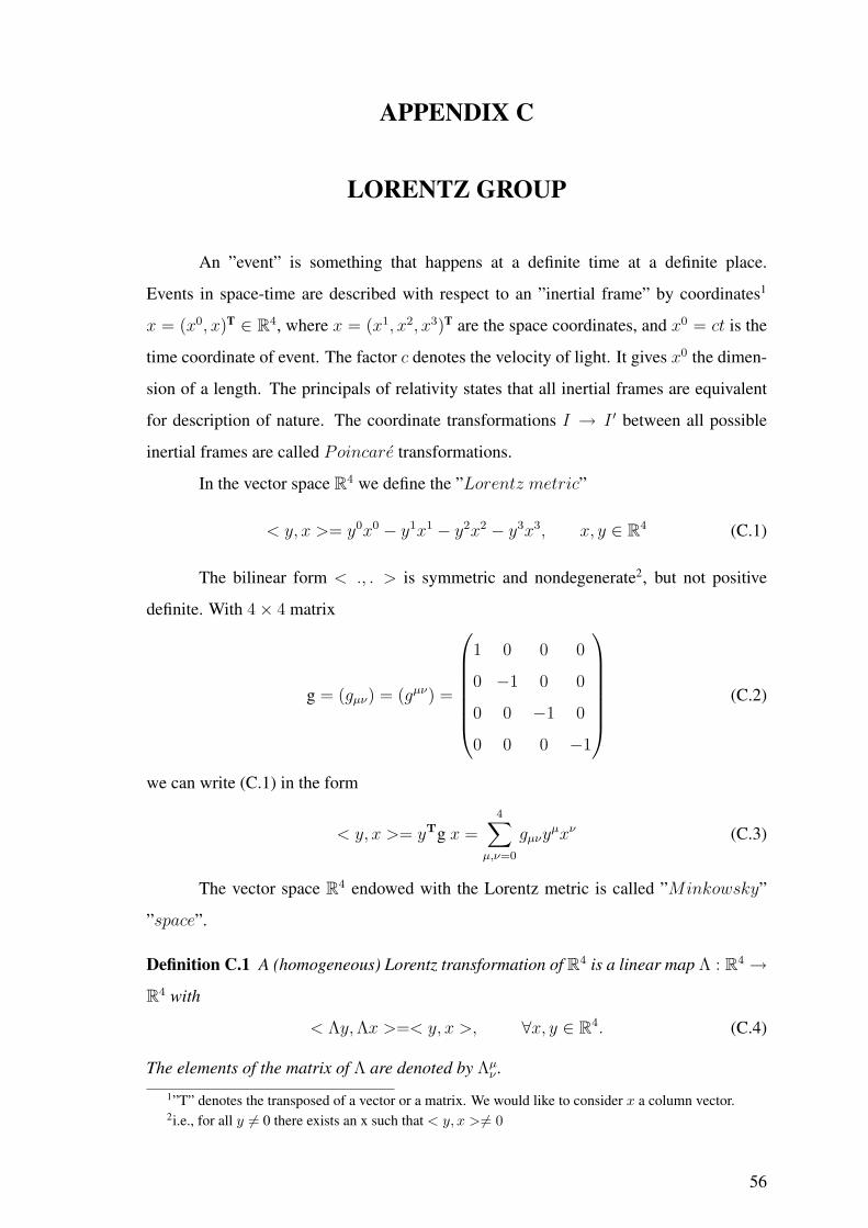
APPENDIX C
LORENTZ GROUP
An ”event” is something that happens at a definite time at a definite place.
Events in space-time are described with respect to an ”inertial frame” by coordinates1
x = (x0, x)T ∈ R4, where x = (x1, x2, x3)T are the space coordinates, and x0 = ct is the
time coordinate of event. The factor c denotes the velocity of light. It gives x0 the dimen-
sion of a length. The principals of relativity states that all inertial frames are equivalent
for description of nature. The coordinate transformations I → I ′ between all possible
inertial frames are called Poincare transformations.
In the vector space R4 we define the ”Lorentz metric”
< y, x >= y0x0 − y1x1 − y2x2 − y3x3, x, y ∈ R4 (C.1)
The bilinear form < ., . > is symmetric and nondegenerate2, but not positive
definite. With 4× 4 matrix
g = (gµν) = (gµν) =
1 0 0 0
0 −1 0 0
0 0 −1 0
0 0 0 −1
(C.2)
we can write (C.1) in the form
< y, x >= yTg x =4∑
µ,ν=0
gµνyµxν (C.3)
The vector space R4 endowed with the Lorentz metric is called ”Minkowsky”
”space”.
Definition C.1 A (homogeneous) Lorentz transformation of R4 is a linear map Λ : R4 →
R4 with
< Λy,Λx >=< y, x >, ∀x, y ∈ R4. (C.4)
The elements of the matrix of Λ are denoted by Λµν .
1”T” denotes the transposed of a vector or a matrix. We would like to consider x a column vector.2i.e., for all y 6= 0 there exists an x such that < y, x > 6= 0
56

Eq. (C.4) is equivalent to
ΛTg Λ = g or ΛµρgµνΛ
ντ = gρτ , (C.5)
which consists of ten independent quadratic equations for the components of Λ, e.g.,
(Λ00)
2 − (Λ10)
2 − (Λ20)
2 − (Λ30)
2 = 1. (C.6)
The composition of two Lorentz transformation Λ is again a Lorentz transformation. We
find
1 = −det g = −detΛTg Λ = −detΛTdet g detΛ = (detΛ)2 (C.7)
and hence det Λ = ±1 for any Lorentz transformation Λ. Therefore Λ is invertible and
set of all Lorentz transformations forms a group which is called ”Lorentz group”.
57

APPENDIX D
GROUP REPRESENTATIONS
Definition D.1 An m-dimensional matrix group D(G) is called a representation of the
given group G, if G is homomorphic to D(G). The element D(R) in D(G), which
is nonsingular, is called the representation matrix of the group element R ∈ G in the
representation D(G).
Definition D.2 If all matrices D(R) in D(G) are unitary, D(G) is called unitary
representation.
Definition D.3 Two representations D(G) and D(G) with the same dimension are called
equivalent to each other if there is a similarity transformation X relating two representa-
tion matrices for each element R in the group G, D(R) = X−1D(R)X .
The concept of equivalence of representations is reflexive, symmetric and transi-
tive: every representation is equivalent to itself; if a representation D(G) is equivalent to
a representation D(G), then D(G) is equivalent to D(G); if D(G) is equivalent to D(G)
and D(G) is equivalent to D(G), then D(G) is equivalent to D(G). Therefore the set
off all representations of the group G can be divided into equivalence classes of represen-
tations. Henceforth we shall not distinguish between equivalent representations, i.e. we
shall study the properties of equivalence classes of representations.
Definition D.4 A representationD(G) of the groupG is said to be reducible if the repre-
sentation matrix D(R) of any elementR of G in D(G) can be transformed into the same
form of the echelon matrix by a common similarity transformation X ,
X−1D(R)X =
D(1)(R) T (R)
0 D(2)R
. (D.1)
Otherwise, it is called an irreducible representation.
The necessary and sufficient condition for a reducible representation is that there is a
nontrivial invariant subspace with respect to D(G) in its representation space. That is,
if a representation possesses only trivial invariant subspaces it is called irreducible. A
representation with nontrivial invariant subspaces is reducible.
58