Four simplified gradient elasticity models for thesimulation of dispersive wave propagation

Harm Askes1∗, Andrei V. Metrikine2, Aleksey V. Pichugin3 and Terry Bennett1

1 Department of Civil and Structural Engineering,University of Sheffield, Sheffield, U.K.

2 Faculty of Civil Engineering and Geosciences,Delft University of Technology, Delft, Netherlands

3 Department of Mathematical Sciences,Brunel University, Uxbridge, U.K.

Philosophical Magazine, 88(28–29), pp. 3415–3443 (2008).

Abstract

Gradient elasticity theories can be used to simulate dispersive wave propagation as it occurs in heterogeneousmaterials. Compared to the second-order partial differential equations of classicaly elasticity, in its most generalformat gradient elasticity also contains fourth-order spatial, temporal as well as mixed spatial-temporal deriva-tives. The inclusion of the various higher-order terms has been motivated through arguments of causality andasymptotic accuracy, but for numerical implementations it is also important that standard discretisation tools canbe used for the interpolation in space and the integration in time. In this paper, we will formulate four differentsimplifications of the general gradient elasticity theory. We will study the dispersive properties of the models,their causality according to Einstein and their behaviour in simple initial/boundary value problems.

1 IntroductionWave propagation through a heterogeneous material is normally dispersive, that is, each harmonic wave componenttravels with a different velocity. In most materials, waves with larger wave numbers travel slower than waves withsmaller wave numbers. Indeed, such dispersive wave propagation has been observed experimentally in a rangeof materials and through a range of scales, as for instance phonon dispersion in Bismuth [1]. When dispersivewave propagation is simulated, the analyst needs to balance accuracy and efficiency of the model. The classicalequations of elasticity are non-dispersive, thus describing the material as homogeneous using classical elasticity isnot an option. A detailed modelling of every heterogeneity in detail is normally prohibitive, but instead so-calledgeneralised continuum theories can be used as an alternative.

Generalised continuum theories describe the material as homogeneous yet they contain additional terms thatcapture the heterogeneities. An important class of generalised continuum theories are the so-called gradient elas-ticity theories, in which the classical stress-strain relations are extended with additional gradients. These theoriesbuild upon the theories of elasticity with microstructure of Mindlin [2] and Toupin [3]. Simplified formats havebeen popularised in the 1990s through the works of Aifantis, e.g. [4] suggested the following constitutive relationwhich was motivated for use in statics

σi j =Ci jkl(εkl − ℓ2εkl,mm

)(1)

where σ and ε are the Cauchy stress and the infinitesimal strain, respectively, C contains the elastic moduli andthe additional parameter ℓ is an internal length scale. The format of Equation (1) has been used successfully to

∗corresponding author; University of Sheffield, Department of Civil and Structural Engineering, Sir Frederick Mappin Building, MappinStreet, Sheffield S1 3JD, email h.askes@sheffield.ac.uk

1

dispose of strain singularities in crack tip analysis [5–8] and dislocation analysis [9–11]. Another class of gradientelasticity theories have been formulated whereby the response of a discrete material model is continualised in orderto capture the dynamic behaviour of heterogeneous materials [12–15]. The commonly obtained format reads

σi j =Ci jkl(εkl + ℓ2εkl,mm

)(2)

where the only difference with Equation (1) concerns the sign of the higher-order term. The advantages of such ap-proaches are that the the internal length scale ℓ is normally straightforwardly identified in terms of the geometry ofthe heterogeneity, e.g. particle spacing, and the dispersive properties of discrete material models are approximatedwith more accuracy compared with classical elasticity. Unfortunately, however, models according to Equation (2)are unstable [16–18]; while they possess some merit in predicting the dispersive properties of materials they shouldnot be used in boundary value problems.

Gradient elasticity theories that can be used in statics (e.g. removal of strain singularities) as well as in dynamics(e.g. realistic prediction of dispersion) should combine the advantages of Equations (1) and (2). Gradient theorieswith higher-order inertia terms fulfill this requirement; a generic format that is an extension of Equation (1) reads[19–24]

σi j =Ci jkl(εkl − ℓ2

s εkl,mm)+ρℓ2

mui, jtt (3)

where two length scales are included: ℓs accompanies the higher-order stiffness term and ℓm accompanies thehigher-order inertia term. The double time derivative of the last term in Equation (3) denotes inertia and should notbe confused with viscosity (which would have been indicated with an odd time derivative). In fact, Equation (3)follows the generic formulation of Mindlin, who proposed a simultaneous extension of the potential energy andthe kinetic energy [2]. Note that the static counterpart of Equation (3) follows Equation (1), not Equation (2).

Although Equation (3) predicts a realistic dispersion of propagating waves, nevertheless further improvementsof Equation (3) have been suggested recently, namely the inclusion of a fourth-order time derivative in the equationsof motion. The case has been argued indepedently in two different ways, namely:

• Metrikine [25] demonstrated that the model according to Equation (3) is non-causal in the sense that energycan propagate faster than the speed of light (albeit with infinitesimal amplitude). To mitigate this, i.e. toretain causality of the formulation, a fourth-order time derivative is required alongside fourth-order spatialderivatives and mixed fourth-order derivatives (twice with respect to time, twice with respect to the spatialcoordinates). It was furthermore shown that such a model can be derived by continualisation of a two-phasematerial.

• Pichugin et al. [26] compared various series expansions and explored their asymptotic equivalence in theconstruction of gradient elasticity theories. The various higher-order derivatives are asymptotically equiv-alent but upon truncation give different approximation errors when compared to the response of a discretemodel. The inclusion of the fourth-order time derivative can be used to improve the asymptotic accuracy ofthe resulting theory.

Independently of the above arguments of causality and asymptotic accuracy, a number of studies have addressedthe formulation of gradient elasticity theories that lend themselves to straightforward numerical implementation,e.g. with finite element methods and standard time integration techniques. The equilibrium equations accordingto Equation (1) are fourth-order and would thus require C 1-continuity of the spatial interpolation. While someprogress in C 1-continuous implementations for gradient theories has been made using Hermitian finite elements[27] and meshless methods [28, 29], another line of research has been to re-formulate gradient elasticity prior todiscretisation such that the usual C 0-continuous shape functions can be used. Ru and Aifantis have suggested anoperator split for gradient elasticity by which two second-order equations are solved sequentially, rather than theoriginal fourth-order equations [6]. Numerical implementations of this approach have been pursued in [30] forstatics and in [31] for dynamics. Other C 0-implementations of gradient elasticity that have been suggested arebased on Pade approximations of Equation (2) [32] and an implementation of the Mindlin theory in which thedifference between micro-displacements and macro-displacements is penalised [33].

This paper focusses on gradient elasticity theories for dispersive wave propagation and their subsequent finiteelement implementation. First, we will briefly revisit in Section 2 a generalised gradient elasticity that includes theterms of Equation (3) as well as the fourth-order time derivative of the displacements. Next, in Section 3 we willfocus on four particular versions of the general model that lend themselves to straighforward implementations,

2

in particular formats that can be implemented using standard finite elements with C 0-continuous interpolationfunctions. In the next three sections we will study the following properties of the four special gradient elasticitymodels, namely dispersion properties (Section 4), causality (Section 5) and the variationally consistent boundaryconditions (Section 6). Numerical examples are presented in Section 7.

2 Formulation of the generic modelIn order to keep this contribution self-contained, the formulation of the generic model that includes all fourth-orderterms is recapped briefly by revisisting the derivations of Pichugin et al. [26]. Starting point is the simple discretemodel depicted in Figure 1. All particles have mass M and all springs have stiffness K. Note that we only considerlongitudinal displacement — this leads to the gradient elasticity models mentioned above, whereas the inclusionof rotational degrees of freedom would result in Cosserat-type models [13, 34, 35].

The equation of motion of the central particle reads

M∂ 2un(t)

∂ t2 = K(

un−1(t)−2un(t)+un+1(t))

(4)

where M and K are the particle mass and the spring stiffness, respectively, both of which are assumed to be uniform.The discrete particle displacements un−1(t), un(t) and un+1(t) are replaced by their continuous counterparts u(x−ℓ, t), u(x, t) and u(x+ ℓ, t). Taylor series are applied to u(x± ℓ, t), by which up to order O

(ℓ2)

the equations ofmotion read

∂ 2u(x, t)∂ t2 = c2

e∂ 2u(x, t)

∂x2 +O(ℓ2) (5)

where ce =√

E/ρ is the elastic bar velocity, while the mass density ρ = M/Aℓ, the Young’s modulus E = Kℓ/Aand A is the cross sectional area. A higher-order approximation of Equation (4) is obtained by including the nextterms of the Taylor series [13, 14, 36], that is

∂ 2u(x, t)∂ t2 = c2

e∂ 2u(x, t)

∂x2 +1

12c2

eℓ2 ∂ 4u(x, t)

∂x4 +O(ℓ4) (6)

As is well-known, Equation (6) is unstable for wave numbers k >√

12/ℓ [16, 20, 37, 38] and should not be usedto solve boundary value problems [16]. The unstable higher-order term in Equation (6) can be replaced by sta-ble higher-order terms as follows: the second derivative with respect to x is taken of Equation (5); the result ismultiplied with C1ℓ

2 and substracted from Equation (6), by which

∂ 2u(x, t)∂ t2 −C1ℓ

2 ∂ 4u(x, t)∂ t2∂x2 = c2

e∂ 2u(x, t)

∂x2 −(

C1 −1

12

)c2

eℓ2 ∂ 4u(x, t)

∂x4 +O(ℓ4) (7)

The resulting equation of motion is stable for all wave numbers provided that the model parameter C1 >112 . Note

that the truncation errors of Equations (6) and (7) are the same, namely O(ℓ4).

Remark 1 The asymptotic equivalence of Equations (6) and (7) has been explored in [37, 38] who used C1 =112 .

Similarly, in [20, 21] a modified relation between the kinematic variables of the discrete model and the continuummodel was defined in the transition from Equation (4) to Equation (7).

xn−2 xn−1 xn xn+1 xn+2

Figure 1: One-dimensional array of particles connected by springs

3

Another asymptotically equivalent formulation was obtained by Pichugin et al. [26] by taking the second timederivative of Equation (5) and multiplying the result with C2ℓ

2/c2e . Adding the obtained expression to Equation (7)

yields

∂ 2u(x, t)∂ t2 +C2

ℓ2

c2e

∂ 4u(x, t)∂ t4 − (C1 +C2)ℓ

2 ∂ 4u(x, t)∂ t2∂x2 =

c2e

∂ 2u(x, t)∂x2 −

(C1 −

112

)c2

eℓ2 ∂ 4u(x, t)

∂x4 +O(ℓ4) (8)

Equation (8) is yet again asymptotically accurate up to O(ℓ4).

Instead of the particle spacing ℓ and the two model parameters C1 and C2, one can also interpret the coefficientsof the higher-order terms as three separate internal length scales. A reformulation of Equation (8) to this extentwould read

∂ 2u(x, t)∂ t2 − c2

e∂ 2u(x, t)

∂x2 +ℓ2

1c2

e

∂ 4u(x, t)∂ t4 − ℓ2

2∂ 4u(x, t)∂ t2∂x2 + c2

eℓ23

∂ 4u(x, t)∂x4 = 0 (9)

where ℓ1 = ℓ√

C2, ℓ2 = ℓ√

C1 +C2 and ℓ3 = ℓ√

C1 − 112 . While these three internal length scales cannot be chosen

independently if the behaviour of Equation (4) is to be approximated, more complicated material models may allowfor independent values of the three length scales, see for instance the continualisation of a three-phase material asstudied by Metrikine [25].

3 Formulation of the special modelsIt is desirable to have a higher-order elasticity theory that not only describes wave dispersion realistically, butthat can also be implemented straightforwardly, i.e. using standard numerical discretisation tools. Here, we willinvestigate special cases of Equation (9) that lend themselves to straightforward finite element implementations.To this end, fourth-order spatial derivatives require special care, and should ideally be replaced by second-orderspatial derivatives. Fourth-order time derivatives can in principle be handled but require an extension of existingnumerical time integration schemes.

3.1 Special model 1: ℓ1 = ℓ3 = 0

The simplest reduction of Equation (9) that is still dispersive can be obtained by setting ℓ1 = 0 (thus avoidingcomplications in the time integration a priori) as well as ℓ3 = 0 (thus avoiding complications with the continuityof the spatial discretisation a priori). The resulting model reads

∂ 2u(x, t)∂ t2 − c2

e∂ 2u(x, t)

∂x2 − ℓ22

∂ 4u(x, t)∂ t2∂x2 = 0 (10)

and this particular format has been suggested by many researchers before in the context of dispersive wave propa-gation, e.g. [37–40]. The only higher-order term is second-order in space (thus, standard finite element techniquescan be used) and second-order in time (this, standard numerical time integration schemes can be used). The dis-persive properties of this model are somewhat unusual in that the phase and group velocities of the shorter wavesapproaches zero and there is a cut-off frequency above which the waves do not propagate (see Section 4). The orig-inal model also acts as a low-pass filter that does not propagate waves with frequencies above a cut-off. Therefore,special model 1 can be considered to capture the filtering property of the original model.

3.2 Special model 2: ℓ3 = 0

As an extension of the previous model, the fourth-order time derivative may be retained. Only the fourth-orderspatial derivative is eliminated by setting its coefficient equal to zero, by which

∂ 2u(x, t)∂ t2 − c2

e∂ 2u(x, t)

∂x2 +ℓ2

1c2

e

∂ 4u(x, t)∂ t4 − ℓ2

2∂ 4u(x, t)∂ t2∂x2 = 0 (11)

The spatial discretisation of this model is straightforward but the time integration algorithm needs adaptations,which are discussed in detail in Appendix B.

4

Remark 2 Pichugin et al. [26] argued that two extra orders of accuracy can be gained for Equation (8) through aspecific choice for C1 and C2, namely C1 =

112 and C2 =

120 . With this parameter choice, special model 2 is obtained

with ℓ1 = ℓ/√

20 and ℓ2 = ℓ√

2/15. Note that there is no clear physical meaning of the numerical coefficients1/√

20 and√

2/15; they merely follow from exploring the equivalence of two asymptotic series.

Remark 3 Due to the presence of two (rather than one) propagating modes as explained in Section 4, specialmodel 2 may produce high-frequency oscillations that are not present in the original chain-model, especially whenthe loading contains substantial high-frequency component. As an approximation of Equation (4) this theory isonly valid for modelling motions dominated by frequencies below the second mode cut-off.

3.3 Special model 3: ℓ1 = 0

Another specialisation of Equation (9) is obtained by omitting the fourth-order time derivative but keeping thefourth-order spatial derivative. Thus,

∂ 2u(x, t)∂ t2 − c2

e∂ 2u(x, t)

∂x2 − ℓ22

∂ 4u(x, t)∂ t2∂x2 + c2

eℓ23

∂ 4u(x, t)∂x4 = 0 (12)

In fact, this model is the one-dimensional equivalent of Equation (3) and its wave propagation characteristics havebeen studied before in [2, 19–22, 24]. The presence of the fourth order spacial derivative means that this modelassociates two wave numbers to each frequency, one of which does not exist in the original model [26]. Thisbecomes particularly important when formulating boundary conditions for this model.

The development of a finite element implementation of this model has been hampered by the inclusion of thefourth-order spatial derivative. To overcome this, an operator split has been developed by which the fourth-orderdifferential equation (12) is rewritten as a set of two second-order differential equations [18, 31], as follows:

• a new displacement-type variable u(x, t) is defined through

u(x, t) = u(x, t)− ℓ23

∂ 2u(x, t)∂x2 (13)

by which Eq. (12) can be rewritten as

∂ 2u(x, t)∂ t2 − ℓ2

2∂ 4u(x, t)∂ t2∂x2 − c2

e∂ 2u(x, t)

∂x2 = 0 (14)

• Take the second time derivative of Equation (13) and multiply with ℓ22/ℓ

23. The result is used to replace the

second term in Equation (14).

• Take the second time derivative of Equation (13) and multiply with 1−ℓ22/ℓ

23. The result is to be used instead

of Equation (13).

• The resulting set of equations is symmetric, fully coupled and contains at most second-order spatial deriva-tives and at most second-order time derivatives:

ℓ22

ℓ23

∂ 2u(x, t)∂ t2 −

ℓ22 − ℓ2

3

ℓ23

∂ 2u(x, t)∂ t2 − c2

e∂ 2u(x, t)

∂x2 = 0 (15)

together with

−ℓ2

2 − ℓ23

ℓ23

∂ 2u(x, t)∂ t2 +

ℓ22 − ℓ2

3

ℓ23

∂ 2u(x, t)∂ t2 −

(ℓ2

2 − ℓ23) ∂ 4u(x, t)

∂ t2∂x2 = 0 (16)

The symmetry issue relates to the coefficient of u in the first equation being equal to the coefficient of u(x, t)in the second equation — this facilitates identifying the underlying energy densities and, in turn, naturalboundary conditions [31].

5

In the derivations the assumption was made that ℓ2 = ℓ3. In case ℓ2 = ℓ3 a model is obtained that is not dispersive(see also Remark 5 below). The fact that the space and time derivatives are at most of order two means that stan-dard discretisation techniques can be used (e.g. the usual C 0-continuous finite elements for spatial discretisationand the standard Newmark scheme for the time integration). From a comparison with Mindlin’s 1964 theory thesecond displacement-type variable u(x, t) has been identified as the microscopic displacement whereas the originaldisplacement variable u(x, t) is the macroscopic displacement [41].

3.4 Special model 4: ℓ22 = ℓ2

1 + ℓ23

The case ℓ22 = ℓ2

1 + ℓ23 allows Equation (9) to be rewritten as(

∂ 2

∂ t2 − c2e

∂ 2

∂x2

)(1+

ℓ21

c2e

∂ 2

∂ t2 − ℓ23

∂ 2

∂x2

)u(x, t) = 0 (17)

In going from Equation (9) to Equation (17), all fourth-order derivatives have been factorised as products of second-order derivatives. Equation (17) can be seen as an operator split in which firstly the equations of classical elasticityare solved, that is

∂ 2uc(x, t)∂ t2 − c2

e∂ 2uc(x, t)

∂x2 = 0 (18)

where uc(x, t) is the displacement according to classical elasticity. The solution of Equation (18) then serves as thesource term for a second equation, i.e.

u(x, t)+ℓ2

1c2

e

∂ 2u(x, t)∂ t2 − ℓ2

3∂ 2u(x, t)

∂x2 = uc(x, t) (19)

In contrast to Equations (15–16), the resulting equations of special model 4 are uncoupled: u(x, t) does not appearin Equation (18). Thus, Equations (18) and (19) can be solved sequentially which is less time-consuming thansolving the fully coupled system of Equations (15) and (16).

Remark 4 In contrast to the previous 3 special models, special model 4 cannot be obtained from Equation (8)through an appropriate choice for C1 and C2. Thus, as an approximation of Equation (4) it is only accurate toorder O(ℓ2). This can be interpreted physically as follows: the first factor in Equation (17) assumes non-dispersivepropagation of the fundamental mode, whereas O(ℓ4) asymptotic accuracy of the dispersion relation of the chaindictates that the fundamental mode must be dispersive [26].

Remark 5 In case ℓ1 = 0 it follows that ℓ2 = ℓ3. This further particularisation of special model 4 is non-dispersive.This can easily be seen as follows: Equation (18) is non-dispersive, and without time derivatives Equation (19)provides merely a smooting of uc(x, t) in the spatial domain, not in the time domain. Equation (23) in the nextSection illustrates this point: the angular frequency would be a linear function of the wave number for such amodel.

4 Dispersion propertiesTo investigate the dispersive properties of the various models, a trial solution u(x, t) = Bexp(i(kx−ωt) is substi-tuted into Equation (9), whereby B is the amplitude, k is the wave number and ω is the angular frequency. Thisresults in

ℓ21

c2e

ω4 −(1+ ℓ2

2k2)ω2 + c2ek2 (1+ ℓ2

3k2)= 0 (20)

For the various models the angular frequency ω can be resolved as

Model 1: ω = cek · 1√1+ ℓ2

2k2(21)

6

0 0.5 1 1.5 2 2.5 3 3.5 4 4.5 50

0.2

0.4

0.6

0.8

1

1.2

1.4

1.6

1.8

2

k [1/mm]

ω [r

ad/s

]

Figure 2: Angular frequency versus wave number for Model 1 (dotted), Model 2 (solid), Model 3 (dash-dotted)and Model 4 (dashed)

Model 2: ω = cek ·

√√√√1+ ℓ22k2 ±

√(1+ ℓ2

2k2)2 −4ℓ2

1k2

2ℓ21k2 (22)

Model 3: ω = cek ·

√1+ ℓ2

3k2

1+ ℓ22k2 (23)

Model 4: ω = cek∨

ω = cek ·

√1+ ℓ2

3k2

ℓ21k2 (24)

These curves of ω versus k are plotted in Figure 2 for ce = 1 m/s and ℓ2 =√

2 m; furthermore ℓ1 = 1 m in Models 2and 4 and ℓ3 = 1 m in Models 3 and 4. All four models have a primary branch in the ω−k plane that passes throughthe origin; these branches were called acoustical branches by Mindlin. In addition, the models with a fourth-ordertime derivative (i.e. Models 2 and 4) also have a secondary branch that starts at a finite cut-off frequency; Mindlindenoted these the optical branches. Three cases can be distinguished concerning the primary (acoustical) branches:

• the curve attains a horizontal asymptote: this happens in case ℓ3 = 0, that is for Models 1 and 2. The impli-cations are that the phase velocity c = ω/k will vanish for the larger wave numbers, i.e. the high-frequencywaves do not propagate. This mimics the low-pass behaviour of the original problem governed by Equa-tion (4), but may be undesirable in the context of other physical problems. However, this must be judgedagainst the fact that spatial discretisation filters out all frequencies higher than a threshold value set by thediscretisation (e.g. by the finite element size).

• the curve attains a non-horizontal asymptote: in case ℓ3 = 0 a non-horizontal asymptote is attained for thelarge wave numbers, the slope of which is governed by the ratio ℓ3/ℓ2. This means that the correspondingphase velocities will be finite for all wave numbers. Such is the case for the present Model 3.

• the curve is a straight line through the origin: for the particular combination of ℓ1, ℓ2 and ℓ3 of Model 4the primary branch is given by ω = cek which happens to be the same as classical elasticity. As such, theprimary branch of Model 4 is associated with the first of the factorised equations, that is expression (18).This particular branch is non-dispersive.

7

As regards the secondary (optical) branches, they start at a cut-off frequency given by ω = ce/ℓ1, and they attainnon-horizontal asymptotes with slopes ceℓ2/ℓ1 (Model 2) and ceℓ3/ℓ1 (Model 4). It is noted that the secondarybranch of Model 4 corresponds to Equation (19).

5 CausalityIt is desirable that mechanical models observe the principle of causality [42] according to which the cause has toprecede its effect. In fact, all models that are formulated in the time domain do satisfy this principle. The causalitymay be violated if the frequency-domain formulation is adopted and the Kramers-Kroenig relations [43] are notobserved. All the above-introduced models are formulated in the time-space domain and, therefore, satisfy thecausality principle.

A stricter requirement than the causality principle is the so-called Einstein’s causality that postulates that signalscan not propagate faster than the speed of light. In classical mechanics, all disturbances propagate with much lowerspeeds and Einstein’s causality may seem to be of no significance. In our view, however, it is desirable that alsoclassical mechanical models observe Einstein’s causality and do not allow signals to propagate energy infinitelyfast. In this section, it is investigated whether the above-introduced gradient elasticity models satisfy Einstein’scausality.

5.1 The wave equationThe wave equation is considered here to demonstrate a method that will be applied to check whether the above-introduced gradient elasticity models observe Einstein’s causality. The method makes use of the Laplace andFourier integral transforms that are defined as follows:

us (x,s) =∞∫

0

u(x, t)exp(−st) dt and us,k (k,s) =∞∫

−∞

us (x,s)exp(ikx) dx (25)

Consider the wave equation with the right-hand side representing a point pulse load:

∂ 2u∂ t2 − c2

e∂ 2u∂x2 = Fδ (x)δ (t) (26)

where F is a constant and δ (...) is the Dirac delta-function. Applying the integral transforms defined by Equation(25) to Equation (26), one obtains

us,k(s2 + c2

ek2)= F ⇒ us,k =F

s2 + c2ek2 (27)

First, the Fourier inversion is applied to Equation (27). Facilitated by the contour integration and the residuetheorem [44], it results in

us =1

2π

∞∫−∞

us,k exp(−ikx) dk =F

2πc2e

∞∫−∞

exp(−ikx)(k− is

/ce)(

k+ is/

ce) dk =

F2sce

exp(− s |x|

ce

)(28)

Next, the inverse Laplace transform [45] is applied:

u(x, t) =1

2πi

a+i∞∫a−i∞

us (x,s)exp(st) ds (29)

where a is a positive real number that is larger than the real parts of all singularities of us (x,s). Insertion of Equation(28) into Equation (29) gives

u(x, t) =F

4πcei

a+i∞∫a−i∞

1s

exp(− s

ce(|x|− cet)

)ds =

12πi

a+i∞∫a−i∞

Z (s) ds (30)

8

s

a

C

leftC

s

a

rightC C

Figure 3: Integration contours in the complex s-plain for |x|> cet (left) and |x|< cet (right)

The integral in Equation (30) can be evaluated using the contour integration and the residue theorem. The integra-tion contours are chosen in the manner shown in Figure 3. Let us first consider |x|< cet and use the contour shownin the left part of Figure 3. According to Cauchy’s residue theorem [44], the following holds

∮Cleft

Z (s) ds =a+i∞∫

a−i∞

Z (s) ds+∫

C−∞

Z (s) ds = 2πi Ress=0

(Z (s)) (31)

where Ress=0

(Z (s)) is the residue of Z (s) at s = 0. Due to Jordan’s lemma [44], the integral over the semicircle C−∞

vanishes as its radius tends to infinity. Therefore,

u(x, t)|x|<cet =1

2πi

a+i∞∫a−i∞

Z (s) ds = Ress=0

(Z (s)) =F

2ce(32)

For |x|> cet, the contour shown in the right part of Figure 3 can be used. As this contour surrounds no singularity,Cauchy’s residue theorem gives

∮Cright

Z (s) ds =a+i∞∫

a−i∞

Z (s) ds+∫

C+∞

Z (s) ds = 0 (33)

Due to Jordan’s lemma, the integral over the infinite semicircle C+∞ is zero and, therefore,

u(x, t)|x|>cet =1

2πi

a+i∞∫a−i∞

Z (s) ds = 0 (34)

Equations (32) and (34) reproduce a well-known result that propagation of disturbances in a medium describedby the one-dimensional wave equation is bounded by two propagating fronts located at |x| = cet. This result isreproduced here to show that existence of the fronts (and, consequently, Einstein’s causality) can be concludedupon by a relatively simple analysis of the argument of the exponent in the inverse Laplace transform, Equation(30). Indeed, the fronts can be associated with the transition of the contour closure (the semicircles in Figure 3)from the left half-plane of the complex s-plain to its right half-plane. This transition, in turn, is associated withthe possibility to close the contour such that the integral along the closure vanishes as its radius tends to infinity.The latter is one-to-one related to the argument of the exponent in the inverse Laplace transform. If in the limitRe(s) → +∞ the real part of this argument tends to minus infinity for |x| > Ct, C > 0 then the fronts exist at|x|=Ct and Einsteins causality is satisfied. This criterion will be used in the following subsections to conclude onEinstein’s causality of special models 1–4.

9

5.2 Special model 1Application of the integral transforms defined by Equation (25) to Equation (10) enriched by Fδ (x)δ (t) on theright-hand side, results in

us,k(s2 + c2

ek2 + ℓ22s2k2)= F ⇒ us,k =

Fs2 + c2

ek2 + ℓ22s2k2 (35)

The inverse Fourier transform is accomplished as follows

us =F2π

∞∫−∞

exp(−ikx)s2 + c2

ek2 + ℓ22s2k2 dk =

F2π

(c2

e + ℓ22s2

) ∞∫−∞

exp(−ikx)(k− k1)(k− k2)

dk (36)

where

k1 =is√

c2e + ℓ2

2s2and k2 =

−is√c2

e + ℓ22s2

(37)

Choosing the branch of the square root in Equation (37) such that the real part of this root is positive in the wholes-plane, one can use the contour integration and evaluate Equation (36) as

us =−2πiF

2π(c2

e + ℓ22s2

) exp(−ik2 |x|)(k2 − k1)

=1

2s√

c2e + ℓ2

2s2exp

− s |x|√c2

e + ℓ22s2

(38)

Application of the inverse Laplace transform to Equation (38) gives

u(x, t) =F

4πi

a+i∞∫a−i∞

1

s√

c2e + ℓ2

2s2exp

−s |x|√c2

e + ℓ22s2

+ st

ds (39)

In the limit Re(s)→+∞ the argument of the exponent in Equation (39) tends to −|x|/ℓ2+ st which makes it clearthat the integral over the infinite semicircle in the right half-plane of the complex s-plane does not vanish for anyx. This means that there are no fronts in model 1 and this model does not observe Einstein’s causality.

Note that the Laplace solution given by Equation (38) differs significantly from that given by Equation (28). Thedifference consists in the existence of the branch points and branch cuts in the complex s-plane that are associatedwith the chosen branch of the square root in Equation (38). However, as the branch points and the branch cuts arelocated at the left of the inverse-Laplace integration contour (the straight vertical line in Figure 3), the criterionbased on the argument of the exponent remains applicable.

5.3 Special model 2The Laplace-Fourier solution of Equation (11) that is subjected to Fδ (x)δ (t) at its right-hand side reads

us,k =F

s2 + c2ek2 + ℓ2

1s4/

c2e + ℓ2

2s2k2(40)

The Fourier inversion can be accomplished in the same manner as for model 1 to give

us =1

2s√

c2e + ℓ2

2s2√

1+ ℓ21s4

/c2

e

exp

−s |x|

√1+ ℓ2

1s4/

c2e√

c2e + ℓ2

2s2

(41)

where the branches of the square roots are chosen such that the real parts of both roots are positive in the wholes-plane. In the limit Re(s)→+∞ the argument of the exponent in the inverse Laplace transform of Equation (41)reads

Arg∞ =

st − s |x|

√1+ ℓ2

1s4/

c2e√

c2e + ℓ2

2s2

Re(s)→+∞

=− sce

(|x| ℓ1

ℓ2− cet

)Re(s)→+∞

(42)

The above argument tends to minus infinity provided that |x| > cetℓ2/ℓ1. Thus, this model observes Einstein’scausality as it predicts signals to propagate no faster than with the speed ceℓ2/ℓ1.

10

5.4 Special model 3The Laplace-Fourier solution for this model is given as

us,k =F

s2 + c2ek2 + ℓ2

2s2k2 + ℓ23c2

ek4 (43)

In contrast to the preceding models, the denominator of this solution has four k-roots. Let us write the expressionsfor these roots directly in the limit Re(s)→+∞. In this limit

k1 =iℓ2, k2 =− i

ℓ2, k3 = i

sce

ℓ2

ℓ3and k4 =−i

sce

ℓ2

ℓ3(44)

Accordingly, the inverse Fourier transform of Equation (43) in this limit can be evaluated as

us =F

2πℓ23c2

e

∞∫−∞

exp(−ikx)(k− k1)(k− k2)(k− k3)(k− k4)

dk

= − iFℓ2

3c2e

(exp(−ik2 |x|)

(k2 − k1)(k2 − k3)(k2 − k4)+

exp(−ik4 |x|)(k4 − k1)(k4 − k2)(k4 − k3)

)Re(s)→+∞

=12

Fs2ℓ2

exp(−|x|

l2

)− 1

2Fceℓ3

s3ℓ32

exp(− s |x|

ce

ℓ3

ℓ2

)(45)

Thus, the inverse Laplace transform should be taken of the two terms, which correspond to the following argumentsof the exponents in the limit Re(s)→+∞:

Arg1∞ = st − |x|ℓ2

and Arg2∞ =− sce

(|x| ℓ3

ℓ2− cet

)(46)

Although Arg2∞ ensures a certain abrupt change at |x|= cetℓ2/ℓ3, Arg1∞ does not tend to minus infinity as Re(s)→+∞. Therefore, this model allows signals to spread infinitely fast and, consequently, it does not observe Einstein’scausality.

5.5 Special model 4The Laplace-Fourier solution for this model is given as

us,k =F

(s2 + c2ek2)

(1+ ℓ2

1s2/

c2e + ℓ2

3k2) (47)

The k-roots of the denominator in the limit Re(s)→+∞ read

k1 =isce, k2 =− is

ce, k3 =

isce

ℓ1

ℓ3and k4 =− is

ce

ℓ1

ℓ3(48)

Accordingly, the inverse Fourier transform of Equation (47) in the limit Re(s)→+∞ can be evaluated as

us =F

2πℓ23c2

e

∞∫−∞

exp(−ikx)(k− k1)(k− k2)(k− k3)(k− k4)

dk

= − iFℓ2

3c2e

(exp(−ik2 |x|)

(k2 − k1)(k2 − k3)(k2 − k4)+

exp(−ik4 |x|)(k4 − k1)(k4 − k2)(k4 − k3)

)Re(s)→+∞

= −12

Fce

s3(ℓ2

3 − ℓ21

) exp(− s |x|

ce

)+

12

Fceℓ3

s3ℓ1(ℓ2

3 − ℓ21

) exp(− s |x|

ce

ℓ1

ℓ3

)(49)

The arguments of the exponents in the inverse Laplace transform, as follows from Equation (49) with Re(s)→+∞,have the following form:

Arg1∞ =− sce

(|x|− cet) , Arg2∞ =− sce

(|x| ℓ1

ℓ3− cet

)(50)

As Re(s)→ +∞, the first and the second arguments tend to minus infinity at |x| > cet and |x| > cetℓ3/ℓ1, respec-tively. Thus, as for the physical validity of this model ℓ3/ℓ1 must be not smaller than unity (see the dispersionanalysis of Section 4), the signals are always confined within the leading fronts |x| = cetℓ3/ℓ1 and the modelobserves Einstein’s causality.

11

6 Boundary conditionsIn order to formulate the consistent boundary conditions of the various models, a variational approach will be takenthat later on straigtforwardly leads to the associated finite element equations. Assuming a domain x ∈ [0,L], theweak form of Equation (9) reads

L∫0

w(x)(

∂ 2u(x, t)∂ t2 +

ℓ21

c2e

∂ 4u(x, t)∂ t4

)dx+

L∫0

∂w(x)∂x

(c2

e∂u(x, t)

∂x+ ℓ2

2∂ 3u(x, t)

∂ t2∂x

)dx

+

L∫0

∂ 2w(x)∂x2 c2

eℓ23

∂ 2u(x, t)∂x2 dx =

[w(x)

(c2

e∂u(x, t)

∂x+ ℓ2

2∂ 3u(x, t)

∂ t2∂x− ℓ2

3c2e

∂ 3u(x, t)∂x3

)]L

0+

[∂w(x)

∂xℓ2

3c2e

∂ 2u(x, t)∂x2

]L

0(51)

where w(x) is an appropriate test function and integration by parts has been applied once and twice for terms withfirst-order spatial derivatives and second-order spatial derivatives, respectively. The right-hand-side of Equation(51) reveals the format of the boundary conditions, namely

either prescribe u(x, t) or prescribe c2e

(∂u(x, t)

∂x− ℓ2

3∂ 3u(x, t)

∂x3

)+ ℓ2

2∂ 3u(x, t)

∂ t2∂x(52)

either prescribe∂u(x, t)

∂xor prescribe ℓ2

3c2e

∂ 2u(x, t)∂x2 (53)

Note that the natural boundary conditions can be expressed in terms of stress-type variables, that is a Cauchy stressσ as

σ = E(

ε − ℓ23

∂ 2ε∂x2

)+ρℓ2

2∂ 2ε∂ t2 (54)

where ε = ∂u(x, t)/∂ t is the uniaxial strain, and a higher-order stress τ as

τ = Eℓ23

∂ε∂x

(55)

As regards the non-standard higher-order boundary conditions, most researchers employ homogeneous naturalboundary conditions, that is setting τ = 0. Essential boundaries were analysed in [46], where it was shown that theboundary conditions of expressions (52) and (53) may result in O(ℓ2) error caused by the presense of boundarylayers in theories with higher-order spacial derivatives. An asymptotic procedure that can reduce this error belowO(ℓ3) is also suggested in [46].

6.1 Special models 1 and 2Special models 1 and 2 are retrieved from the original model by a specific choice of parameters, without furthermanipulations. Thus, the boundary conditions for these two models can be retrieved as well from the boundaryconditions of the original model. Note that there is only one essential boundary condition and only one naturalboundary conditions in these two models, that is, expression (53) does not apply.

6.2 Special model 3In the formulation of special model 3, a few manipulations have been made by which the boundary conditions areaffected. To find their appropriate format, the weak form of Equations (15–16) is taken, that is

L∫0

w(x)(ℓ2

2

ℓ23

∂ 2u(x, t)∂ t2 −

ℓ22 − ℓ2

3

ℓ23

∂ 2u(x, t)∂ t2

)dx+

L∫0

∂ w(x)∂x

c2e

∂ u(x, t)∂x

dx =[

w(x)c2e

∂ u(x, t)∂x

]L

0(56)

12

andL∫

0

w(x)(−ℓ2

2 − ℓ23

ℓ23

∂ 2u(x, t)∂ t2 +

ℓ22 − ℓ2

3

ℓ23

∂ 2u(x, t)∂ t2

)dx+

L∫0

∂w(x)∂x

(ℓ2

2 − ℓ23) ∂ 3u(x, t)

∂ t2∂xdx

=

[w(x)

(ℓ2

2 − ℓ23) ∂ 3u(x, t)

∂ t2∂x

]L

0(57)

where again integration by parts has been applied to terms with spatial derivatives. From the right-hand-sides ofEquations (56) and (57) the boundary conditions are found as

either prescribe u(x, t) or prescribe c2e

∂ u(x, t)∂x

= c2e

(∂u(x, t)

∂x− ℓ2

3∂ 3u(x, t)

∂x3

)(58)

either prescribe u(x, t) or prescribe(ℓ2

2 − ℓ23) ∂ 3u(x, t)

∂ t2∂x(59)

Note that the two natural boundary conditions of special model 3 together constitute the Cauchy stress as given inEquation (54), albeit with a different factor accompanying the higher-order inertia term.

Although the model is derived from a format that includes a fourth-order spatial derivative, there are no higher-order stresses present in this model and expression (53) does not apply. However, it is possible to emulate theeffects of the higher-order stresses by setting a tying between the degrees of freedom u and u. That is, by settingu(x, t) = u(x, t) on the boundary it is implicitly set through Equation (13) that

ℓ23

∂ 2u(x, t)∂x2 = 0 (60)

on the boundary, which is equivalent to setting the higher-order stress τ equal to zero on the boundary.

6.3 Special model 4In special model 4, the mechanical equations are treated in two consecutive steps. Firstly, Equation (18) is solvedand it is accompanied by the usual boundary conditions of classical elasticity, that is

either prescribe uc(x, t) or prescribe c2e

∂uc(x, t)∂x

(61)

To retrieve the boundary conditions corresponding to the second step, the weak form of Equation (19) is taken.Integration by parts of the term with spatial derivatives yields

L∫0

w(x)(

u(x, t)+ℓ2

1c2

e

∂ 2u(x, t)∂ t2

)dx+

L∫0

∂w(x)∂x

ℓ23

∂u(x, t)∂x

dx =[

w(x)ℓ23

∂u(x, t)∂x

]L

0+

L∫0

w(x)uc(x, t)dx (62)

so that the boundary conditions are found as

either prescribe u(x, t) or prescribe ℓ23

∂u(x, t)∂x

(63)

This model is the only special model to retain all terms that appear in the original model of Equation (9). It is thusof interest to compare the boundary conditions given through expressions (52–53) with those in expressions (61)and (63). The first essential and natural boundary conditions in both models are stated in terms of a displacementand a Cauchy-type stress. However, the second essential boundary condition contains a strain-type variable inexpression (53) in contrast to the displacement variable in expression (63). Similarly, the second natural boundarycondition contains a higher-order stress in expression (53) in contrast to a strain-type variable in expression (63).

Clearly, there is a mismatch between the two sets of boundary conditions. A simple way to amend this is totake the spatial derivative of Equation (19), that is

ε(x, t)+ℓ2

1c2

e

∂ 2ε(x, t)∂ t2 − ℓ2

3∂ 2ε(x, t)

∂x2 =∂uc(x, t)

∂x(64)

in which the strain ε is the primary unknown. The boundary conditions accompanying Equation (64) are

either prescribe ε(x, t) or prescribe ℓ23

∂ε(x, t)∂x

(65)

which are compatible with those given in expression (53).

13

F

Figure 4: One-dimensional dynamic bar problem — geometry and loading conditions

0 10 20 30 40 50 600

0.5

1

1.5

x [mm]

ε [−

]

40 50 60 70 80 90 1000

0.5

1

1.5

x [mm]

ε [−

]

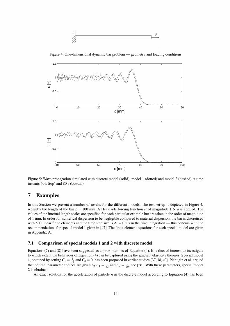
Figure 5: Wave propagation simulated with discrete model (solid), model 1 (dotted) and model 2 (dashed) at timeinstants 40 s (top) and 80 s (bottom)

7 ExamplesIn this Section we present a number of results for the different models. The test set-up is depicted in Figure 4,whereby the length of the bar L = 100 mm. A Heaviside forcing function F of magnitude 1 N was applied. Thevalues of the internal length scales are specified for each particular example but are taken in the order of magnitudeof 1 mm. In order for numerical dispersion to be negligible compared to material dispersion, the bar is discretisedwith 500 linear finite elements and the time step size is ∆t = 0.2 s in the time integration — this concurs with therecommendations for special model 1 given in [47]. The finite element equations for each special model are givenin Appendix A.

7.1 Comparison of special models 1 and 2 with discrete modelEquations (7) and (8) have been suggested as approximations of Equation (4). It is thus of interest to investigateto which extent the behaviour of Equation (4) can be captured using the gradient elasticity theories. Special model1, obtained by setting C1 =

112 and C2 = 0, has been proposed in earlier studies [37, 38, 40]. Pichugin et al. argued

that optimal parameter choices are given by C1 =112 and C2 =

120 , see [26]. With these parameters, special model

2 is obtained.An exact solution for the acceleration of particle n in the discrete model according to Equation (4) has been

14

0 50 1000

1

2

0 50 1000

1

2

0 50 1000

1

2

0 50 1000

1

2

0 50 1000

1

2

0 50 1000

1

2

0 50 1000

1

2

0 50 1000

1

2

Figure 6: Wave propagation simulated with model 3 — microscopic strain (left) and macroscopic strain (right)across bar for times 20 s, 40 s, 60 s and 80 s. Boundary conditions have not been corrected. Dotted lines indicatethe analytical solution for classical elasticity.

given in [48] and reads

an(t) =2n−1

tJ2n−1(2t) (66)

where J is the Bessel function of the first kind of order 2n− 1. In Figure 5 this exact solution is compared to thesolutions of special models 1 and 2 for time instants 40 s and 80 s, whereby we have taken a particle spacingℓ = 1 mm. Thus, ℓ1 = 0 and ℓ2 = 1/

√12 mm for model 1, whereas for model 2 we have ℓ1 = 1/

√20 mm and

ℓ2 =√

2/15 mm. Generally, there is a good correspondence between the three solutions, especially around thewave front. Compared to special model 1, special model 2 captures the slow travelling higher frequencies of thediscrete model somewhat better.

7.2 Influence of boundary conditions in models 3 and 4Next, the importance of using homogeneous higher-order natural boundary conditions is demonstrated for specialmodels 3 and 4. Whereas models 1 and 2 are found from the original model of Equation (9) through a suitableselection of values for the various length scales, models 3 and 4 are obtained through a number of mathematicalmanipulations. As a result, the natural consistent boundary conditions of models 3 and 4 are different from thoseof the original model, although amendments have been suggested in Section 6. These boundary conditions andtheir suggested improvement are studied in the same problem as above, whereby the length of the bar L = 100m, Young’s modulus E = 1 N/m2 and mass density ρ = 1 kg/m3. The length scales ℓ2 = 2 m and ℓ3 = 1 m for

15

0 50 1000

1

2

0 50 1000

1

2

0 50 1000

1

2

0 50 1000

1

2

0 50 1000

1

2

0 50 1000

1

2

0 50 1000

1

2

0 50 1000

1

2

Figure 7: Wave propagation simulated with model 3 — microscopic strain (left) and macroscopic strain (right)across bar for times 20 s, 40 s, 60 s and 80 s. Boundary conditions have been corrected by setting u = u. Dottedlines indicate the analytical solution for classical elasticity.

model 3, while ℓ1 = ℓ3 = 1 m for model 4. The bar is discretised with 200 linear finite elements and for the timeintegration a time step size of 0.5 s is used.

Firstly, special model 3 is considered. At the free end, the natural boundary conditions of expressions (58)and (59) are used, that is ∂ u/∂x = 1 and ∂ 3u/∂ t2∂x = 0. It was suggested in Section 6 to emulate zero higher-order stresses on the boundary by setting a relation between the microscopic displacement u and the macroscopicdisplacement u as u(x, t) = u(x, t). Without this amendment, the microscopic and macroscopic strain profiles asdepicted in Figure 6 are obtained, whereby the two strain fields are plotted along the bar for successive timeinstants. It can be seen that the microscopic strain (depicted on the left of Figure 6) attains realistic values at theboundary where the force is applied. In contrast, the macroscopic strain (depicted on the right) unrealistically tendsto zero at the left end of the bar. If the amendment u(x, t) = u(x, t) is adopted, the results of Figure 7 are obtained.It can be seen that for this case, the value of the macroscopic strain at the left end is realistic. This demonstrates theimportance of using zero higher-order stress on the boundaries in special model 3. Interestingly, the microscopicstrains are affected as well: compared to Figure 6, the microscopic strains in Figure 7 are much smoother.

Next, special model 4 is considered. For every time step, two sets of equations must be solved consecutively.The first set of equations are those of classical elasticity, and for the second set two options exist, either in termsof displacements as in Equation (19) or in terms of strains as in Equation (64). Figures 8 and 9 show the strainprofiles along the bar for successive time instants. The results of Equation (18) are also shown — they do not differin the two Figures. Yet again, the importance of using zero higher-order stresses on the boundaries is evident. InFigure 8 the strains following from Equation (19), and using ∂u/∂x = 0 as a boundary condition, attain unrealistic

16

0 50 1000

1

2

0 50 1000

1

2

0 50 1000

1

2

0 50 1000

1

2

0 50 1000

1

2

0 50 1000

1

2

0 50 1000

1

2

0 50 1000

1

2

Figure 8: Wave propagation simulated with model 4 — strains for classical elasticity (left) and gradient elasticity(right) across bar for times 20 s, 40 s, 60 s and 80 s. Boundary conditions have not been corrected. Dotted linesindicate the analytical solution for classical elasticity.

values at the left end of the bar. In contrast, the strains according to Equation (64), and obtained with the boundarycondition ∂ε/∂x = 0, are realistic as is demonstrated in Figure 9.

7.3 Parameter restriction in model 4In Section 4 the dispersive properties of the various special models were presented. For model 4, the existenceof two branches prohibits certain combinations of parameters. In particular, ambiguities arise if the two branches

cross. This may happen if ℓ1 > ℓ3, in which case the ambiguous wave number k = 1/√

ℓ21 − ℓ2

3. The correspondingwave length λ is found as

λ =2πk

= 2π√ℓ2

1 − ℓ23 (67)

Figure 10 shows the strain profile evolution for an admissible set of parameters, that is ℓ1 = 1 m and ℓ3 = 2 m.Compared to the case ℓ1 = ℓ3 (such as the case depicted in Figure 9), the strain profiles for ℓ3 > ℓ1 are extremelysmooth. However, the situation changes dramatically for an inadmissible set of parameters. In Figure 11 the resultsare shown for ℓ1 = 2 m and ℓ3 = 1 m. The response is dominated by a single harmonic, of which the amplitude istwice the amplitude of the input signal and the wavelength is given by Equation (67) — in this case, λ ≈ 11 m whichis in excellent correspondence with the wave length of the signal observed in Figure 11 (right). This phenomenonis sometimes denoted “internal resonance” and it is emphasized that its occurrence here is completely unphysical.

17

0 50 1000

1

2

0 50 1000

1

2

0 50 1000

1

2

0 50 1000

1

2

0 50 1000

1

2

0 50 1000

1

2

0 50 1000

1

2

0 50 1000

1

2

Figure 9: Wave propagation simulated with model 4 — strains for classical elasticity (left) and gradient elasticity(right) across bar for times 20 s, 40 s, 60 s and 80 s. Boundary conditions have been corrected by using Equation(64). Dotted lines indicate the analytical solution for classical elasticity.

7.4 Comparison of special models 1–4Finally, the four special models will be compared against one another. The parameter choice of Figure 2 is adoptedhere, that is ℓ1 = ℓ3 = 1 m and ℓ2 =

√2 m. The same bar problem as above is taken, and in Figure 12 the strain

profiles are depicted for all four models and for time instants t = 40 s and t = 80 s. The most important observationis the qualitative differences between models 1–3 on the one hand and model 4 on the other hand. The higherwave numbers are travelling faster in model 4 than in the other models — in fact, they are travelling with virtuallythe same velocity as the lower frequencies. Thus, the dispersive properties of model 4 are much less pronouncedthan those of models 1–3, as already seen in Section 4. The other three models, special models 1–3, differ mainlyquantitatively from each other. In all these three models, the lower wave numbers travel faster than the higher wavenumbers. The flattening of the wave front is most visible in special model 3.

8 Concluding remarksWe have presented four simplified gradient elasticity models that can be used to simulate dispersive wave prop-agation. The four models are obtained through specific values of the various internal length scales of a genericgradient elasticity formulation that contains three higher-order terms: a fourth-order spatial derivative, a fourth-order time derivative and a mixed fourth-order derivative. The special models are formulated such that they can beimplemented using standard finite element procedures.

18

0 50 1000

1

2

0 50 1000

1

2

0 50 1000

1

2

0 50 1000

1

2

0 50 1000

1

2

0 50 1000

1

2

0 50 1000

1

2

0 50 1000

1

2

Figure 10: Wave propagation simulated with model 4 — strains for classical elasticity (left) and gradient elasticity(right) across bar for times 20 s, 40 s, 60 s and 80 s with ℓ1 = 1 m and ℓ3 = 2 m.

The four models have been compared in terms of their dispersive behaviour and whether they fulfil Einstein’scausality. The dispersive properties of special model 4 are limited in that only the secondary (optical) branch ofthe curve frequency versus wave number is dispersive; the primary (acoustical) branch is non-dispersive. The otherthree models exhibit realistic dispersion behaviour. Special models 2 and 4 are strictly causal whereas specialmodels 1 and 3 are not. The causality of the various models is related to the existence of a secondary dispersioncurve; if this secondary, optical branch exists and positive real frequencies are obtained for the limit of infinitelylarge wave numbers, then the model is causal. The variationally consistent boundary conditions have also beenpresented. For the two special models that are based on a fourth-order spatial derivative (special models 3 and 4),particular attention has been paid to the higher-order boundary conditions. For both models, straightforward andsimple amendments have been suggested so as to emulate the effects of zero higher-order stress on the boundary.The importance of such boundary conditions has been demonstrated for both models — failure to impose thecorrect boundary conditions leads to remarkably similar unrealistic results in the two models.

A final verdict depends on which property is deemed most important. Special model 1 is the simplest from thepoints of view of implementation and formulation of boundary conditions. Special model 2 is to be preferred ifcausality is a critical issue. Compared to these two models, special model 3 offers the attractive feature that thepropagation velocity of the higher frequency components can be controlled. Although special model 4 retains allthree length scales that are present in the original formulation, its dispersive properties are minimal compared tothe other three models.

19

0 50 1000

1

2

0 50 1000

1

2

0 50 1000

1

2

0 50 1000

1

2

0 50 1000

1

2

0 50 1000

1

2

0 50 1000

1

2

0 50 1000

1

2

Figure 11: Wave propagation simulated with model 4 — strains for classical elasticity (left) and gradient elasticity(right) across bar for times 20 s, 40 s, 60 s and 80 s with ℓ1 = 2 m and ℓ3 = 1 m.

AcknowledgementsFinancial support of the Engineering and Physical Sciences Research Council to the first author and the fourthauthor (contract number EP/D041368/1) is gratefully acknowleged.

A Spatial discretisation aspectsAll special models have been rewritten as partial differential equations that are second-order in space, hence spatialdiscretisation is straightforward. In this section, the spatially discretised systems of equations are treated briefly.

A.1 Special model 1The spatial discretisation of special model 1 has been treated in [49] and results in[

M0 + ℓ22M1

] ∂ 2u∂ t2 +Ku = f (68)

in which u and f contain the nodal displacements and the externally applied nodal forces, respectively. Moreover,two mass matrices are defined as

M0 =

L∫0

NT ρNdx (69)

20

0 10 20 30 40 50 600

0.5

1

1.5

x [mm]

ε [−

]

40 50 60 70 80 90 1000

0.5

1

1.5

x [mm]

ε [−

]

Figure 12: Wave propagation simulated with model 1 (dotted), model 2 (solid), model 3 (dash-dotted) and model4 (dashed) at time instants 40 s (top) and 80 s (bottom)

M1 =

L∫0

∂NT

∂xρ

∂N∂x

dx (70)

and the stiffness matrix is given through

K =

L∫0

∂NT

∂xE

∂N∂x

dx (71)

A.2 Special model 2The spatially discretised version of special model 2 is a straightforward extension of Equation (68), i.e.[

M0 + ℓ22M1

] ∂ 2u∂ t2 +

ℓ21

c2e

M0∂ 4u∂ t4 +Ku = f (72)

A.3 Special model 3The spatial discretisation of special model 3 has been treated in detail in [31]; in its final version it reads

ℓ22

ℓ23

M0 −ℓ2

2 − ℓ23

ℓ23

M0

−ℓ2

2 − ℓ23

ℓ23

MT0

ℓ22 − ℓ2

3

ℓ23

M0 +(ℓ2

2 − ℓ23)

M1

∂ 2u∂ t2

∂ 2u∂ t2

+

[K 00 0

][uu

]=

[f0

](73)

where it has been assumed that the same shape functions are used for the interpolation of u and u.

21

A.4 Special model 4Special model 4 consists of two steps. Firstly, the discretised nodal displacements of classical elasticity uc areobtained from

M0∂ 2uc

∂ t2 +Kuc = f (74)

Afterwards, this solution is used as input in the second equation by which the gradient-dependent nodal displace-ments u are found:[

H0 + ℓ23H1

]u+

ℓ21

c2e

H0∂ 2u∂ t2 = H0uc (75)

where

H0 =

L∫0

NT Ndx (76)

H1 =

L∫0

∂NT

∂x∂N∂x

dx (77)

In case the second step of the model is expressed in terms of strains rather than displacements, cf. Equation (64),the right-hand-side of Equation (75) is replaced by

∫NT ∂N

∂x dx uc.

B Numerical time integration of special model 2For the numerical time integration of Equation (11) an extension of the average acceleration variant of the Newmarkscheme is developed. It is assumed that, within the time interval [t, t+∆t] an average value of the nodal fourth-ordertime derivatives c can be defined as

cav ≡12(ct + ct+∆t) (78)

This quantity is then used in successive integration to obtain the nodal third-order time derivatives b, the nodalaccelerations a, the nodal velocities v and, ultimately, the nodal displacements u as

bt+∆t = bt + cav∆t (79)

at+∆t = at +bt∆t +12

cav∆t2 (80)

vt+∆t = vt +at∆t +12

bt∆t2 +16

cav∆t3 (81)

ut+∆t = ut +vt∆t +12

at∆t2 +16

bt∆t3 +124

cav∆t4 (82)

References[1] Y.L. Yarnell, J.L. Warren, R.G. Wenzel, and S.H. Koenig. Phonon dispersion curves in bismuth. IBM J. Res.

Dev., 8:234–240, 1964.

[2] R.D. Mindlin. Micro-structure in linear elasticity. Arch. Rat. Mech. Analysis, 16:52–78, 1964.

[3] R.A. Toupin. Theories for elasticity with couple-stress. Arch. Rat. Mech. Analysis, 17:85–112, 1964.

[4] E.C. Aifantis. On the role of gradients in the localization of deformation and fracture. Int. J. Engng. Sci.,30:1279–1299, 1992.

22

[5] S.B. Altan and E.C. Aifantis. On the structure of the mode III crack-tip in gradient elasticity. Scripta Metall.Mater., 26:319–324, 1992.

[6] C.Q. Ru and E.C. Aifantis. A simple approach to solve boundary-value problems in gradient elasticity. ActaMech., 101:59–68, 1993.

[7] D.J. Unger and E.C. Aifantis. The asymptotic solution of gradient elasticity for mode-III. Int. J. Fract.,71:R27–R32, 1995.

[8] B.S. Altan and E.C. Aifantis. On some aspects in the special theory of gradient elasticity. J. Mech. Behav.Mat., 8:231–282, 1997.

[9] M.Y. Gutkin and E.C. Aifantis. Screw dislocation in gradient elasticity. Scripta Mater., 35:1353–1358, 1996.

[10] M.Y. Gutkin and E.C. Aifantis. Edge dislocation in gradient elasticity. Scripta Mater., 36:129–135, 1997.

[11] M.Y. Gutkin and E.C. Aifantis. Dislocations in the theory of gradient elasticity. Scripta Mater., 40:559–566,1999.

[12] C.S. Chang and J. Gao. Wave propagation in granular rod using high-gradient theory. ASCE J. Engng. Mech.,123:52–59, 1997.

[13] H.-B. Muhlhaus and F. Oka. Dispersion and wave propagation in discrete and continuous models for granularmaterials. Int. J. Solids Struct., 33:2841–2858, 1996.

[14] A.S.J. Suiker, de Borst R., and Chang C.S. Micro-mechanical modelling of granular material. Part 1: Deriva-tion of a second-gradient micro-polar constitutive theory. Acta Mech., 149:161–180, 2001.

[15] H. Askes and A.V. Metrikine. Higher-order continua derived from discrete media: continualisation aspectsand boundary conditions. Int. J. Solids Struct., 42:187–202, 2005.

[16] H. Askes, A.S.J. Suiker, and L.J. Sluys. A classification of higher-order strain gradient models — linearanalysis. Arch. Appl. Mech., 72:171–188, 2002.

[17] J.S. Yang and S.H. Guo. On using strain gradient theories in the analysis of cracks. Int. J. Fract., 133:L19–L22, 2005.

[18] H. Askes and E.C. Aifantis. Gradient elasticity theories in statics and dynamics — a unification of approaches.Int. J. Fract., 139:297–304, 2006.

[19] H.G. Georgiadis, I. Vardoulakis, and G. Lykotrafitis. Torsional surface waves in a gradient-elastic half-space.Wave Mot., 31:333–348, 2000.

[20] A.V. Metrikine and H. Askes. One-dimensional dynamically consistent gradient elasticity models derivedfrom a discrete microstructure. Part 1: Generic formulation. Eur. J. Mech. A/Solids, 21:555–572, 2002.

[21] H. Askes and A.V. Metrikine. One-dimensional dynamically consistent gradient elasticity models derivedfrom a discrete microstructure. Part 2: Static and dynamic response. Eur. J. Mech. A/Solids, 21:573–588,2002.

[22] H.G. Georgiadis. The mode III crack problem in microstructured solids governed by dipolar gradient elastic-ity: static and dynamic analysis. ASME J. Appl. Mech., 70:517–530, 2003.

[23] I.M. Gitman, H. Askes, and E.C. Aifantis. The representative volume size in static and dynamic micro-macrotransitions. Int. J. Fract., 135:L3–L9, 2005.

[24] A.V. Metrikine and H. Askes. An isotropic dynamically consistent gradient elasticity model derived from a2D lattice. Phil. Mag., 86:3259–3286, 2006.

[25] A.V. Metrikine. On causality of the gradient elasticity models. J. Sound Vibr., 297:727–742, 2006.

23

[26] A.V. Pichugin, H. Askes, and A. Tyas. Asymptotic equivalence of homogenisation procedures and fine-tuningof continuum theories. J. Sound Vibr., 313:858–874, 2008.

[27] A. Zervos, P. Papanastasiou, and I. Vardoulakis. A finite element displacement formulation for gradientelastoplasticity. Int. J. Numer. Meth. Engng., 50:1369–1388, 2001.

[28] H. Askes and E.C. Aifantis. Numerical modeling of size effect with gradient elasticity — formulation,meshless discretization and examples. Int. J. Fract., 117:347–358, 2002.

[29] Z. Tang, S. Shen, and S.N. Atluri. Analysis of materials with strain-gradient effects: A Meshless LocalPetrov-Galerkin(MLPG) approach, with nodal displacements only. Comp. Mod. Engng. Sci., 4:177–196,2003.

[30] L.T. Tenek and E.C. Aifantis. A two-dimensional finite element implementation of a special form of gradientelasticity. Comp. Model. Engng. Sci., 3:731–741, 2002.

[31] H. Askes, T. Bennett, and E.C. Aifantis. A new formulation and C0-implementation of dynamically consistentgradient elasticity. Int. J. Numer. Meth. Engng., 72:111–126, 2007.

[32] H. Askes and M.A. Gutierrez. Implicit gradient elasticity. Int. J. Numer. Meth. Engng., 67:400–416, 2006.

[33] A. Zervos. Finite elements for elasticity with microstructure and gradient elasticity. Int. J. Numer. Meth.Engng., 72:564–595, 2008.

[34] A.S.J. Suiker, A.V. Metrikine, and R. de Borst. Comparison of wave propagation characteristics of theCosserat continuum and corresponding lattice models. Int. J. Solids Struct., 38:1563–1583, 2001.

[35] E. Pasternak and H.-B. Muhlhaus. Generalised homogenisation procedures for granular materials. J. Engng.Math., 52:199–229, 2005.

[36] C.S. Chang and J. Gao. Second-gradient constitutive theory for granular material with random packingstructure. Int. J. Solids Struct., 32:2279–2293, 1995.

[37] M.B. Rubin, P. Rosenau, and O. Gottlieb. Continuum model of dispersion caused by an inherent materialcharacteristic length. J. Appl. Phys., 77:4054–4063, 1995.

[38] W. Chen and J. Fish. A dispersive model for wave propagation in periodic heterogeneous media based onhomogenization with multiple spatial and temporal scales. ASME J. Appl. Mech., 68:153–161, 2001.

[39] Z.-P. Wang and C.T. Sun. Modeling micro-inertia in heterogeneous materials under dynamic loading. WaveMot., 36:473–485, 2002.

[40] I.V. Andrianov, J. Awrejcewicz, and R.G. Barantsev. Asymptotic approaches in mechanics: new parametersand procedures. ASME Appl. Mech. Rev., 56:87–110, 2003.

[41] T. Bennett, I.M. Gitman, and H. Askes. Elasticity theories with higher-order gradients of inertia and stiffnessfor the modelling of wave dispersion in laminates. Int. J. Fract., 148:185–193, 2007.

[42] M. Bunge. Causality; the place of the causal principle in modern science. Harvard University Press, 1959.

[43] J.S. Toll. Causality and the dispersion relation: Logical foundations. Physical Review, 104:1760–1770, 1956.

[44] B.A. Fuchs, B.V. Shabat, and J. Berry J. Functions of complex variables and some of their applications.Pergamon, 1964.

[45] M. Abramowitz and I.A. Stegun. Handbook of mathematical functions; with formulas, graphs, and mathe-matical tables. Dover, 1970.

[46] J.D. Kaplunov and A.V. Pichugin. On rational boundary conditions for higher-order long-wave models. InF.M. Borodich, editor, IUTAM Symposium on Scaling in Solid Mechanics, pages 81–90. Springer, 2008. ISBN978-1-4020-9032-5.

24

[47] H. Askes, B. Wang, and T. Bennett. Element size and time step selection procedures for the numericalanalysis of elasticity with higher-order inertia. J. Sound Vibr., 314:650–656, 2008.

[48] H. Bavinck and H.A. Dieterman. Closed-form dynamic response of damped massspring cascades. J. Comput.Appl. Math., 114:291–303, 2000.

[49] J. Fish, W. Chen, and G. Nagai. Non-local dispersive model for wave propagation in heterogeneous media:one-dimensional case. Int. J. Numer. Meth. Engng., 54:331–346, 2002.

25