fouling of exhaust gas recirculation coolers · 2019-07-13 · fouling of exhaust gas recirculation...
TRANSCRIPT

Fouling of Exhaust Gas
Recirculation Coolers
DEUTZ AG
Sara Raquel Gonçalves Guedes de Pinho Guerra
A thesis submitted for the degree of
Master of Science in Mechanical Engineering to the
Faculty of Engineering, University of Porto
Porto, July 2017
Supervisor at FEUP: Prof. Dr. Carlos Pinho
Supervisor at DEUTZ AG: Dr.-Ing. Andreas Boemer

[Blank Page]
“Das Gleiche läßt uns in Ruhe, aber der Widerspruch ist es, der uns
produktiv macht.“
„Uniformity gives us serenity, but contradiction is what makes us
productive”
Johann Wolfgang von Goethe


Abstract As the human species faces aggravating climate changes and the world’s natural
resources are being consumed at an incredibly fast rate, government policies struggle to
find ecological and economical solutions that can prevent catastrophic outcomes.
In this scope, engine exhaust gas emissions are one of the biggest concerns in the
current days, as the use of fossil fuels and non-renewable energy sources is taking a toll
on our planet. Therefore, these legal policies are aimed to reduce the level of greenhouse
gas emissions that contribute to the climate alterations.
The introduction of Exhaust Gas Recirculation (EGR) coolers in the functioning of diesel
engines plays a very important role in reducing exhaust gas emissions and has for
several decades been a theme of deep study. Contributing for the study of these
components is DEUTZ AG, the company that manufactured the first motor engine, back
in 1864.
This work focuses on a detailed study of the effect of fouling in Exhaust Gas
Recirculation (EGR) coolers, its causes and the consequences that it has on the
performance of these components. This analysis was achieved by the performance of
simulations in the Computation Fluid Dynamics (CFD) Software ANSYS Fluent, with the
contribution of C-routines provided by ATLANTING GmbH. These simulations allowed to
conclude which factors have a greater impact in the functioning of these heat exchangers
and also to assess the validity of the routines provided for this study.
This dissertation was carried out at DEUTZ AG in Cologne, Germany, within the
framework of the Dissertation for the Master Degree in Mechanical Engineering at the
Faculty of Engineering of the University of Porto (FEUP), Portugal, with a specialization
in the field of Thermal Energy.

Resumo A espécie humana tem vindo a enfrentar alterações climáticas cada vez mais agravantes
e os recursos naturais to planeta têm vindo a ser consumidos a uma velocidade
alarmante. Como tal, políticas governamentais têm sido desenvolvidas de modo a
encontrar soluções ecológicas e económicas que possam prevenir resultados
catastróficos.
Neste âmbito, as emissões de gases provenientes dos motores de combustão interna são
uma das maiores preocupações atuais, uma vez que o uso de combustíveis fósseis e de
recursos energéticos não renováveis tem um severo impacto no nosso planeta.
A introdução de EGR coolers no funcionamento dos motores a diesel desempenha um
papel muito importante na redução de emissões de gases de combustão e tem vindo a
ser tema de grande estudo nas últimas décadas. Um dos contribuidores para o estudo
destes componentes é a DEUTZ AG, a primeira empresa a fabricar motores a combustão
interna, em 1864.
Este trabalho foca-se no estudo detalhado do efeito do sujamento nos EGR coolers, as
suas causas e as consequências que provoca no desempenho destes componentes. Esta
análise foi conseguida através da realização de simulações com o software de CFD ANSYS
Fluent, com a contribuição de rotinas em código C fornecidas pela empresa ATLANTING
GmbH. Estas simulações permitiram concluir que fatores têm maior influência no
funcionamento destes permutadores de calor e também discernir a validade das rotinas
fornecidas para este estudo.
Esta dissertação foi realizada nas infraestruturas da DEUTZ AG em Colónia, na
Alemanha, no âmbito da Dissertação para obtenção do grau de Mestre em Engenharia
Mecânica, pela Faculdade de Engenharia da Universidade do Porto (FEUP), com uma
especialização em Energia Térmica.

Acknowledgments I would like to take an opportunity to express my gratitude to the following
persons, who contributed for the achievement and completion of this dissertation:
First and foremost, to my parents and my brother, who made me the person I am
today and always empowered and impelled me to pursue my dreams and ambitions;
without whom I would not have had the chance to come abroad and fulfil my goals; for
their unconditional support; for their joy to live and see me thrive.
To my close friends in Porto, whose support was remarkable, tireless and crucial,
even miles apart; I am so glad to have you by my side.
To my javalis, the ones who walked alongside me for these last five years, which
were, so far, the best ones of my life. To the memories I will never remember with
people I will never forget. For all that we have shared, I am glad to have shared it with
you; I wouldn’t have had it with anyone else. It has been a hell of a ride!
To my German girls, for being the most welcoming and warm-hearted people I
could have asked for; Köln acquired a special beauty thanks to you. To my Jule, for being
so tireless and supportive; my everyday saviour.
I would like to express my utmost gratitude to Professor Dr. Carlos Pinho, whose
guidance was the solid basis that allowed me to properly structure my work and do not
lose sight of what is important; for his encouragement and dedication.
A special thanks to Dr. -Ing. Andreas Boemer and his team, from DEUTZ AG, for
providing me with the chance to write my Master Thesis in an industrial context, and to
Mr. Vedder from Atlanting GmbH; whose dedication and patience made this work
possible and made me grow and overcome the obstacles I encountered.
A word of appreciation to Dr. -Ing. Peter Völk, for having the kindness to answer
my many questions and for providing me with his thesis, which granted me a better
foundation for the completion of my dissertation.
To the city of Porto, my hometown, for being a paradise by the ocean and the best
place to have grown in; no matter how beautiful the world is, there is nothing like home.

Finally, a word of appreciation to the Faculty of Engineering, at the University of
Porto (FEUP), which has been my second home throughout this entire journey, and has
provided me with the chance to become an Engineer and to follow my dreams.
Obrigada!

Index of Contents
1. Introduction .............................................................................................................................................. 1
2. Literature Review ................................................................................................................................... 5
2.1. DEUTZ AG – Company Overview ............................................................................................. 5
2.2. EGR Coolers ...................................................................................................................................... 6
2.2.1. European Legislation for Gas emissions ...................................................................... 6
2.2.2. Technology Overview .......................................................................................................... 7
2.3. Fouling ............................................................................................................................................. 11
2.4. Fouling Mechanisms .................................................................................................................. 13
2.4.1. Thermophoresis ................................................................................................................. 13
2.4.2. Diffusiophoresis .................................................................................................................. 17
2.4.3. Condensation ....................................................................................................................... 18
2.4.4. Impaction............................................................................................................................... 19
2.4.5. Diffusion ................................................................................................................................. 20
2.5. Influence of Flow State .............................................................................................................. 22
2.6. Deposit Characteristics and Fouling Consequences ...................................................... 23
2.7. Removal Mechanisms ................................................................................................................ 26
2.7.1. Condensation ....................................................................................................................... 27
2.7.2. Gas flow shear stress......................................................................................................... 28
2.7.3. Kinetic Energy ..................................................................................................................... 29
2.7.4. Oxidation/Evaporation .................................................................................................... 30
3. Thermodynamic Analysis of Fouling ............................................................................................ 31
4. Computational Fluid Dynamics ...................................................................................................... 33
4.1. Introduction – Fluent Approach ............................................................................................ 33
4.1.1. Governing Equations ......................................................................................................... 34
4.2. Turbulence Analysis .................................................................................................................. 35
4.2.1. k-ε model ............................................................................................................................... 37
4.2.2. k-ω model .............................................................................................................................. 38
4.3. Wall Treatment ............................................................................................................................ 39
4.4. Conjugate Heat Transfer .......................................................................................................... 42
4.5. CFD Coupling using UDF .......................................................................................................... 43
4.6. Errors in CFD Calculations ...................................................................................................... 46
5. Method – Model Validation .............................................................................................................. 47
5.1. Geometry ........................................................................................................................................ 47
5.2. Mesh Characteristics and Influence ..................................................................................... 48
5.3. Exhaust Gas Composition ........................................................................................................ 50
5.4. Sulphur Concentration .............................................................................................................. 50
5.5. Soot Particles in Exhaust Gas ................................................................................................. 52
5.6. Motor Test Bench ........................................................................................................................ 60
5.7. Model Test Bench ........................................................................................................................ 61
6. Simulation Parameters ...................................................................................................................... 63
6.1. Features obtained by the UDFs .............................................................................................. 64
6.1.1. Deposit Thickness .............................................................................................................. 64
6.1.2. Deposition Rates ................................................................................................................. 65
6.1.3. Deposition Efficiency ........................................................................................................ 65
6.1.4. Condensation Rates ........................................................................................................... 67
6.1.5. Fouling Factor ...................................................................................................................... 67
6.1.6. Thermal Conductivity ....................................................................................................... 67
6.2. Influence of Particle Size .......................................................................................................... 68
6.3. Influence of Layer Increment Parameter ........................................................................... 69
7. Simulations and Results .................................................................................................................... 73
7.1. Simulations – Model Test Bench ........................................................................................... 73
7.2. Results of Single Effect Variation .......................................................................................... 75
7.2.1. Variation of water temperature .................................................................................... 76
7.2.1. Variation of exhaust gas temperature ........................................................................ 77
7.2.2. Variation of HC concentration ....................................................................................... 82
7.2.3. Variation of H2O concentration ..................................................................................... 85
7.2.4. Variation of SO2 concentration...................................................................................... 88
7.2.5. Variation of the exhaust mass flow ............................................................................. 93
7.2.6. Variation of the soot mass flow .................................................................................... 96
7.3. Sticking Factor .............................................................................................................................. 97
7.4. Simulations – Motor Test Bench .........................................................................................100
7.4.1. Verification of Reynolds number ...............................................................................108
7.4.2. Comparison with time-dependent results ..............................................................108

8. Conclusions and Future Work ......................................................................................................113
8.1. Conclusions .................................................................................................................................113
8.2. Future Work ................................................................................................................................115
References .....................................................................................................................................................117

Index of Figures
Figure 2.1 - Evolution of the Emission Standards in Europe, regarding PM and NOx levels
for Diesel HD engine (Johnson, 2008) ..................................................................................................... 7
Figure 2.2 - SFOC, NOx, HC and CO as a function of EGR rate (Lamas et al., 2013) ................ 9
Figure 2.3 - (A) - High pressure EGR system; (B) - Low pressure EGR system
(Ghassembaglou and Torkaman, 2016) .............................................................................................. 10
Figure 2.4 - Description of the thermal resistance evolution with fouling (Abd-Elhady et
al., 2011) .......................................................................................................................................................... 11
Figure 2.5 - Scheme of fouling process on the cooler wall (Ford, 2011) ................................ 12
Figure 2.6 - Scheme of the thermophoresis effect (Priesching et al., 2015) .......................... 13
Figure 2.7 – Two correlations between the Knudsen number and thermophoretic
coefficient (Völk and Hörnig, 2011) ...................................................................................................... 16
Figure 2.8 - Scheme of the diffusiophoresis caused by a concentration gradient (adapted)
(Völk and Hörnig, 2012) ............................................................................................................................ 17
Figure 2.9 - Scheme of deposition due to impaction (Atlanting, 2016) .................................. 19
Figure 2.10 - Scheme of deposition through diffusion (Atlanting, 2016) ............................... 20
Figure 2.11 - Comparison of deposition velocities for submicron particles at 600K ........ 22
Figure 2.12 - Result of the plugging effect with a lacquer-like deposit for a half-lifetime
used cooler (Lance et al., 2014) .............................................................................................................. 25
Figure 2.13 - Scheme of the forces acting on a particle sticking to the surface (Abarham
et al., 2010) ..................................................................................................................................................... 26
Figure 2.14 - Evolution of the critical flow velocity per particle diameter regarding
removal by shear stress (Abd-Elhady et al., 2011) ......................................................................... 29
Figure 2.15 - Evolution of the fouling resistance of an EGR cooler as a function of gas
velocity (through Re number) ................................................................................................................. 30
Figure 2.16: Scheme of the evolution of particle removal through evaporation (Han et al.,
2015) ................................................................................................................................................................. 30
Figure 3.1 - Scheme of concentric tubes forming a heat exchanger and the associated
thermal resistances (Çengel, 2003) ....................................................................................................... 32
Figure 4.1 - Turbulent flow with highlight on the small and large eddies (Sofialidis,
2013) ................................................................................................................................................................. 36
Figure 4.2 - Scheme of the three different layers composing the near-wall region (ANSYS,
2016b) .............................................................................................................................................................. 40
Figure 4.3 - Scheme of the two near-wall treatment methods (ANSYS, 2016b) .................. 41
Figure 4.4: Example of CHT calculation (Huc, 2014) ...................................................................... 42
Figure 5.1: Layout of the cooler design for field tests used by Völk and Hörnig (2012) .. 47
Figure 5.2 - Screenshot of the mesh used in Fluent for the chosen cooler geometry ........ 49
Figure 5.3 - Zoom-in on the final mesh used for the inside of the tube, 1/4 of the radial
cross-section displayed .............................................................................................................................. 49
Figure 5.4 - Distribution of the concentration of the number of particles for the different
types of soot emitted, per mobility diameter (Völk and Hörnig, 2011) .................................. 53
Figure 5.5 - Frequency and cumulative distribution of a normal distribution (Stieß,
2008) ................................................................................................................................................................. 54
Figure 5.6 - Scheme of the calculation of the area of each of the classes chosen to obtain
the cumulative mass particle distribution .......................................................................................... 56
Figure 5.7 - Cumulative Mass Fraction Curves for Diesel and Flame Soot ............................. 57
Figure 5.8 - Approximation curves to the cumulative mass fractions of the model test
bench ................................................................................................................................................................. 58
Figure 5.9 - Approximation curves to the cumulative mass fractions of the motor test
bench ................................................................................................................................................................. 59
Figure 5.10 - Schematic setup of the model test bench (adapted) (Völk and Hörnig, 2011)
............................................................................................................................................................................. 61
Figure 6.1 - Vapor pressure curves for every single species considered for the exhaust
gas in the routines (Atlanting, 2016) .................................................................................................... 64
Figure 6.2 - Graphic displaying the evolution of deposition rate for particle class P3 with
three different layer increments ............................................................................................................ 70
Figure 6.3 - Evolution of the deposition rate of particle class P3 for operating point K .. 71
Figure 6.4 - Evolution of the deposition rate of particle class P3 in the first six iterations
for operating point K ................................................................................................................................... 71
Figure 7.1 - Evolution of the deposit thickness and deposition efficiency with the
variation of water temperature for test case K ................................................................................. 76
Figure 7.2 - Evolution of the deposit thickness and deposition efficiency with the
variation of exhaust gas temperature at 20 °C of water temperature and constant mass
flow for test case K ....................................................................................................................................... 78

Figure 7.3 - Evolution of the deposit thickness and deposition efficiency with the
variation of exhaust gas temperature at 20 °C of water temperature with respective
mass flow variation for test case K ........................................................................................................ 80
Figure 7.4 - Evolution of the deposit thickness and deposition efficiency with the
variation of HC concentration for test case K .................................................................................... 83
Figure 7.5 - Evolution of the deposit thickness and deposition efficiency with the
variation of H2O concentration for test case K .................................................................................. 85
Figure 7.6 - Evolution of the deposit thickness and deposition efficiency with the
variation of exhaust mass flow for test case K .................................................................................. 94
Figure 7.7 - Evolution of the deposit thickness and deposition efficiency with the
variation of soot mass flow for test case K ......................................................................................... 97
Figure 7.8 - Evolution of the sticking factor with the variation of HC concentration, for
test case K, after 6 iterations .................................................................................................................... 99
Figure 7.9 - Results of Deposit Thickness for Test Case 1 (adapted to English) ................100
Figure 7.10 - Results of Deposit Thickness for Test Case 2 (adapted to English) .............100
Figure 7.11 - Deposited mass for the four water temperature cases of Test Case 1 in
motor test bench from Völk and Hörnig (2011) .............................................................................101
Figure 7.12 - Plot of the simulated evolution of deposit thickness throughout the entire
cooler length for Test Case 1 at 20 °C of water temperature, with 350 ppm of HC and 2%
of H2O .............................................................................................................................................................102
Figure 7.13 - Plot of the evolution of deposit thickness throughout the entire cooler
length for test case 1 at 20 °C of water temperature, with 450 ppm of HC and 11% of H2O
...........................................................................................................................................................................104
Figure 7.14 - Evolution of the deposit thickness for 4.5 kg/h mass flow, with exhaust
temperature of 300 °C and water temperature of 80 °C .............................................................106
Figure 7.15 - Evolution of the thermal conductivity with the exhaust mass flow
throughout the time in the measurements of Völk (2014) ........................................................111

Fouling of Exhaust Gas Recirculation Coolers
Index of Tables
Table 2.1 - Main constituents of diesel exhaust gas (Hörnig, 2012, Völk and Hörnig,
2012) .................................................................................................................................................................... 6
Table 2.2 - EU Emission Standards for heavy-duty Diesel engines in g/kWh (Abd-Elhady
et al., 2011) ........................................................................................................................................................ 7
Table 2.3 - Coefficients of the Antoine equation for the four condensate forming species
............................................................................................................................................................................. 28
Table 4.1 – Property values of pure soot for the deposits ............................................................ 44
Table 5.1 - Description of the values adopted for the thermal conductivity, specific heat
capacity and dynamic viscosity of the exhaust gas for a piece-wise linear evolution ....... 50
Table 5.2 - Values of sulphur and respective conversions to SO2 and H2SO4 used in both
test benches .................................................................................................................................................... 51
Table 5.3 - Mass fractions associated to flame soot – model test bench - to be used as
input for the UDFs ........................................................................................................................................ 58
Table 5.4 - Mass fractions associated to diesel soot from motor test bench to be used as
input for the UDF .......................................................................................................................................... 59
Table 5.5 - Exhaust gas data for the three different EGR-Rates used in model test bench
by Völk and Hörnig (2011) ....................................................................................................................... 60
Table 5.6 - Description of the main input parameters for Test Cases 1 and 2 of motor test
bench ................................................................................................................................................................. 61
Table 5.7 - Description of the several operating points used at the motor test bench by
Völk and Hörnig (2011) ............................................................................................................................. 62
Table 6.1 - Parameters introduced in the UDFs................................................................................ 63
Table 6.2 - Values of the molecular weight of the condensate forming species used in the
routines ............................................................................................................................................................ 67
Table 6.3 - Thermal conductivity associated with each of the condensate species
(Atlanting, 2017) .......................................................................................................................................... 68
Table 7.1- Operating points from the model test bench chosen to perform simulations 73
Table 7.2 - Result values for the deposition efficiency obtained in the measurements by
Völk and Hörnig (2011) for the five chosen operating points .................................................... 74

Fouling of Exhaust Gas Recirculation Coolers
Table 7.3 - Results obtained for the simulations of the five chosen operating points from
the model test bench and the values of deposition efficiency and outlet temperature
from Völk and Hörnig (2011) .................................................................................................................. 74
Table 7.4 - Original results obtained for the simulations of point K ........................................ 75
Table 7.5 - Results on the variation of the water-side temperature for test case K ........... 76
Table 7.6 - First results on the variation of the exhaust gas temperature for test case K 77
Table 7.7 - Values for the mass and volume flows and density for point K ........................... 78
Table 7.8 - Density and mass flow values at constant volume flow from test case K at 400
°C ......................................................................................................................................................................... 79
Table 7.9 - Results of the mass flow change pursued regarding the exhaust gas
temperature variation for test case K ................................................................................................... 79
Table 7.10 - Results on the single variation of HC concentration for point K ....................... 82
Table 7.11 - Ratio between the values of the thermal conductivity and deposit thickness
for the HC different concentrations ....................................................................................................... 84
Table 7.12 - Results on the single variation of H2O concentration for point K ..................... 85
Table 7.13 - Condensation rates from the variations of water concentration values........ 86
Table 7.14 - Results on the interface temperature between deposit layer and the flow, for
variation of water concentration............................................................................................................ 87
Table 7.15 - Display of the different variation attempts regarding the sulphur
concentration ................................................................................................................................................. 88
Table 7.16 - Results of the variation of sulfuric acid concentration on point K, with an
inlet temperature of 100 °C ...................................................................................................................... 89
Table 7.17 - Results of the variation of sulfuric acid concentration on point K, with an
inlet temperature of 150 °C ...................................................................................................................... 89
Table 7.18 - Results of the variation of sulfuric acid concentration on point K, with an
inlet temperature of 200 °C ...................................................................................................................... 90
Table 7.19 - Results of the forces acting in the cooler for the different sulphur
concentrations at 100 °C of exhaust gas inlet temperature ......................................................... 90
Table 7.20 - Results of the mass flow rates from the deposition mechanisms in the cooler
for the different sulphur concentrations at 100 °C of exhaust gas inlet temperature, for
particle size P3............................................................................................................................................... 91
Table 7.21 - Condensation rates of the four different species for the variation of sulphur
concentration at 100 °C with the presence of water ...................................................................... 91

Fouling of Exhaust Gas Recirculation Coolers
Table 7.22 - Results for the variation of sulphur concentration values, with null
concentration of water vapor in the exhaust gas ............................................................................. 92
Table 7.23 - Results on the single variation of exhaust mass flow for point K ..................... 93
Table 7.24 - Condensation rates of the HC present in the flow, for exhaust mass flow
variation of test case K ............................................................................................................................... 95
Table 7.25 - Results on the single variation of soot mass flow for point K ............................ 96
Table 7.26 - Determined values for the sticking factor concerning solely SO2
concentration, after six iterations, for test case K ........................................................................... 98
Table 7.27 - Determined values for the sticking factor concerning solely HC
concentration, after six iterations, for test case K ........................................................................... 99
Table 7.28 - Results for Test Case 1 from motor test bench, with 350 ppm of HC and 2%
of H2O, and the respective results from Völk and Hörnig (2011) ............................................102
Table 7.29 - Results for Test Case 1 from motor test bench, with 450 ppm of HC and 11%
of H2O ..............................................................................................................................................................104
Table 7.30 - Simulation results for 4.5 kg/h mass flow, with exhaust temperature of 300
°C and water temperature of 80 °C ......................................................................................................107
Table 7.31 - Results of the values of Re obtained from the simulations ...............................108
Table 7.32 – Comparison of the simulated values and the measurement values from a
20-hour study for the temperature at the wall and the transferred heat for Test Case 1
...........................................................................................................................................................................109
Table 7.33 - Comparison of the simulated values and the measurement values from an 8-
hour study for the thermal conductivity for Test Case 1, with variation of water
temperature between 60 °C and 80 °C ...............................................................................................110
Table 7.34 - Results obtained from the simulations for the values of thermal conductivity
on the variation of exhaust mass flow, for 80 °C on Test Case 1 ..............................................112
Table 7.35 - Analysis of the ratios between soot and exhaust mass flow .............................112

Fouling of Exhaust Gas Recirculation Coolers
Nomenclature
Symbol Designation Units
A Cooler cross-section area m2
𝐶𝑐 Cunningham correction factor
CFD Computational Fluid Dynamics
CHT Conjugate heat transfer
𝑐𝑝 Specific heat capacity at constant pressure [J/(kg K)]
𝑑𝑝 Particle diameter [m]
𝐷𝑝 Diffusion coefficient
DPF Diesel Particulate Filter
EGR Exhaust Gas Recirculation
𝐹𝐷 Drag force [N]
𝐹𝐿 Lift force [N]
𝐹𝑡ℎ Thermophoretic force [N]
𝐹𝑉 Van der Waals force [N]
𝐹𝑊 Weight of the particle [N]
HC Hydrocarbon
ℎ𝑖 Convective heat transfer coefficient in the flow [W/(m2 K)]
k Thermal conductivity of a given material [W/(m K)]
Kn Knudsen number
𝐾𝑡ℎ Thermophoretic coefficient
l Molecular mean free path [m]
L Macroscopical physical length of interest [m]
𝐿𝑐𝑜𝑜𝑙𝑒𝑟 Cooler characteristic length [m]
�̇� Mass flow rate [kg/s]
M Molecular weight [kg/kmol]
Nu Nusselt number
P Perimeter [m]
PM Particulate Matter
Pr Mean flow Prandtl number
�̇� Transferred heat flux [W]
Q(x) Cumulative particle distribution
q(x) Frequency particle distribution
𝑝𝑣𝑎𝑝 Vapour pressure [kPa]

Fouling of Exhaust Gas Recirculation Coolers
Re Reynolds number
Rf Thermal resistance of fouling layer [m2K/W]
𝑟𝑝 Particle radius [m]
Sc Schmidt number
St Stokes number
SFOC Specific Fuel Oil Consumption [g/kWh]
SST Shear Stress Transport
𝑇𝑖𝑛𝑡𝑒𝑟𝑓𝑎𝑐𝑒 Temperature at the interface of the deposit layer [°C, K]
U Overall heat transfer coefficient [W/(m2 K)]
u Particle velocity [m/s]
𝑉𝐷 Velocity of deposition due to eddy diffusion [m/s]
𝑉𝐷𝑃 Velocity of deposition due to diffusiophoresis [m/s]
𝑉𝑡 Velocity of deposition due to impaction [m/s]
𝑉𝑡ℎ Thermophoretic drift velocity [m/s]
𝑦𝑔𝑖 Molar fraction at the interface of the deposit layer
y+ Dimensionless height of the first cell at the wall
List of Greek Symbols
Symbol Designation Units
δ Deposit layer thickness [m]
ε Soot deposition efficiency [-,%]
휀𝑐𝑜𝑜𝑙𝑒𝑟 Effectiveness of the heat exchanger [-,%]
휀(𝑑𝑝) Deposition efficiency for each particle diameter [-,%]
휀𝑛 Deposition efficiency on the cooler length [-,%]
𝜆, 𝜆𝑓𝑜𝑢𝑙𝑖𝑛𝑔 Deposit layer thermal conductivity [W/(m K)]
𝜆𝑝 Mean free path of gas molecules [m]
𝜆𝑡𝑢𝑏𝑒 EGR cooler tube thermal conductivity [W/(m K)]
μ Dynamic viscosity of the mean flow [kg/(m s)]
υ Gas kinematic viscosity [m2/s]
ρ Density of the mean flow [kg/m3]
𝜏 Particle Relaxation time [s]

Fouling of Exhaust Gas Recirculation Coolers
[Blank Page]

Fouling of Exhaust Gas Recirculation Coolers
1
1. Introduction
Background
The development of the industry throughout the centuries has led to a stage where the
engine industry is subdued to ever stricter gas emission laws, which lead the engine
manufacturers to develop and enhance their engines’ performances, where DEUTZ AG
stands and is propelled to take action. Particularly in diesel engines, the requirements
are high regarding the emission of nitrogen oxides and particulate matter.
The exhaust gas recirculation stands as a possibility to reduce NOx emissions in order to
abide the legal standards on its emissions. And to optimize the engine performance and
increase its efficiency, the introduction of a cooling device becomes necessary, as the
recirculated exhaust gas needs to be cooled before re-entering the cylinders. The
increasing volume specific performance of modern engines requires a better cooling
performance in increasingly smaller spaces (Morsch, 2016).
On the one hand, the cooling of the exhaust gas to be introduced in the engine leads to
lower combustion temperatures, which decreases the amount of NOx emissions. On the
other hand, the high EGR rates will also lead to a higher production of soot components,
so a compromise has to be met (Völk and Hörnig, 2011).
This device that cools down the exhaust gases – EGR cooler –, before they re-enter the
engine, is a heat exchanger which commonly uses water as the cooling fluid. Due to the
temperature gradient between the hot exhaust gases and the wall of the cooler,
condensate forming species such as hydrocarbons and acids lead to the appearance of an
adhesive isolative layer at the wall of the cooler, where particulate matter and ashes also
get attached. This deposit layer reduces the efficiency of the EGR cooler throughout its
lifetime and ought, therefore, to be studied (Hörnig, 2012).

Fouling of Exhaust Gas Recirculation Coolers
2
The physical effective mechanisms that lead and contribute to the emerging of the
isolative layer in this cooling device – the fouling effect - are studied in detail throughout
this dissertation.
The study of these phenomena and the optimization of the performance of the EGR
coolers has had a great contribution due to the Computational Fluid Dynamics (CFD)
analysis. DEUTZ AG uses this type of software to develop its EGR coolers and improve
the ultimate performance of its engines. In this ambit, this dissertation was developed at
DEUTZ AG in Cologne, Germany, for the study of the fouling of EGR coolers through the
help of the CFD software ANSYS Fluent.
Objectives
The primal objective of this dissertation was to analyse several C-routines provided by
Atlanting GmbH and ascertain their validity and applicability at DEUTZ AG, as
customized functions to associate with Fluent in a CFD analysis of the fouling of EGR
coolers. This will be accomplished by testing the routines with several test cases from a
detailed source for boundary conditions, having as a foundation a single basic geometry
to validate the functions to be associated with the CFD simulation. Several more specific
objectives can be outlined, for a better understanding of the conducting line of this
thesis:
• Detailed study of the fouling phenomenon and the causes that lead to it or
attenuate it along with the effects of its occurrence;
• Limitations and software features that improve the study of the particular case
of heat exchangers;
• Characterization of the C-routines and their particular contribution for this
work;
• Definition of a valid and simple geometry for simulation and validation of the
routines in question for the assessment of fouling effects;
• Ascertaining all the boundary conditions necessary for the correct conduction of
the simulations;
• Study of the parameters that play a big role in the final results, and how to
faithfully replicate them, such as the particle distribution in the exhaust gas and
empirical factors embedded in the code that alter the final results;

Fouling of Exhaust Gas Recirculation Coolers
3
• Simulation of the test cases provided with several approaches regarding single
variable variations in order to understand their behavior and influence on the
evolution of the fouling effect.
The consequent results obtained from these simulations will be then compared to the
experimental values from the sources provided, in order to estimate their accuracy and
usability for the study of EGR coolers at DEUTZ AG.
Throughout the simulation phase the fluid used in the cooling process was always water;
consequently, it will not be continually specified. The routines provided allow for the
calculation of the final state of equilibrium, which represents the fouling effect under
long term condition, that is, at an infinite length of time, where the time no longer plays
any role. This is valid for the CHT and Fouling analysis, as later will be explained.
All the CFD simulations performed in the scope of this study were executed in the
commercial Software ANSYS Fluent, version 17.0. The underlying objective of this thesis
was to develop solid knowledge on CFD simulations and the behavioral analysis of fluid
flows.
Thesis Outline
The outline of this thesis consists of nine main chapters: [1] introduction, [2] a brief
review on the company where this dissertation was developed and the work achieved
by it throughout the years and a literature review, [3] a thermodynamic analysis of the
fouling effect, [4] an introduction to CFD and the parameters associated to it that are
more relevant for this thesis, [5] a layout of the model used for the simulations and its
prime features which allowed a correct replication of the values provided from the main
sources, [6] the simulation parameters used and the ones that generated a greater
influence in the final results, which were the biggest concern throughout this thesis, in
order to accomplish viable results, [7] the display of the simulations performed and the
respective achieved results, [8] the assessment of all the work done and final remarks,
with an insight of what could the future work contemplate regarding the theme of this
thesis.

Fouling of Exhaust Gas Recirculation Coolers
4
[Blank Page]

Fouling of Exhaust Gas Recirculation Coolers
5
2. Literature Review
2.1. DEUTZ AG – Company Overview
DEUTZ AG takes the pride in being the first founded engine company, back in 1864,
having developed the first combustion engine to be produced in a large scale: an
atmospheric gas engine. Looking back on over 150 years of history, DEUTZ AG has
produced cars, trucks, locomotives, tractors and, of, course, their engines (DEUTZ,
2017).
Nowadays it has specialized in the production of Diesel and Gas combustion engines for
several fields of application, such as industrial and construction machinery, gensets,
agricultural machinery, marine and automobile engines. Its engines’ power output
ranges from 12 to 500 kW, either with air, water or oil-cooling systems.
As the legislations regarding gas emissions become ever stricter, DEUTZ AG is put under
pressure to develop better, more effective and more compact engines, emitting fewer
emissions. For that to happen, the cooling system of the engines must be improved, and
for modern combustion engines, smaller and more compact coolers with better
performance are requested. This stands on the fact that a better cooling performance
leads to a better usage of the heat produced by the engine (Morsch, 2016).
Therefore, one of the great investments DEUTZ AG undertakes is in the study and
development of the coolers’ performance with the aid of Computational Fluid Dynamics
(CFD) software. In this line of thought, this work was a contribution for this process, as a
study of the heat transfer and consequent fouling effect occurring in the EGR-Coolers for
Diesel engines.

Fouling of Exhaust Gas Recirculation Coolers
6
Although air used to be the main cooling fluid for combustion engines, today the state of
the art are water-cooled engines. The advantages of the latter one are undeniable, as it
provides a higher heat transfer coefficient and therefore, more heat can be dissipated
from the exhaust gas; also, being beneficial when developing more compact coolers, as
the water properties are much more suitable than air properties to endure the thermal
strains occurring in this process.
2.2. EGR Coolers
2.2.1. European Legislation for Gas emissions
Diesel engine emissions are a major threat agent to the environment and human health,
both in terms of global warming and carcinogenic action of these elements. This is
especially critical concerning nitrogen oxides NOx, CO2 and particulate matter (PM). The
common emissions from a Diesel engine are depicted in Table 2.1,
Exhaust gas component At idle At high load
Nitrogen oxide (NOx) 50 – 100 ppm 600 – 2000 ppm
Hydrocarbon (HC) 50- 500 ppm < 50 ppm
Carbon monoxide (CO) 100 – 450 ppm < 300 ppm
Carbon dioxide (CO2) until 3.5 Vol-% about 12 Vol.-%
Water vapor (H2O) 2 – 4 Vol.-% until 11 Vol-%
Oxygen (O2) 18 Vol.-% 4 - 8 Vol.-%
Soot content - passenger
vehicles < 50 mg m-3 50 – 120 mg m-3
Table 2.1 - Main constituents of diesel exhaust gas (Hörnig, 2012, Völk and Hörnig, 2012)
Therefore, stricter limits regarding these emissions have been issued throughout the
years, requiring the engine manufacturing industry a great effort to meet them, Table 2.2
(Walenbergh, 2003).

Fouling of Exhaust Gas Recirculation Coolers
7
Figure 2.1 - Evolution of the Emission Standards in Europe, regarding PM and NOx levels for Diesel HD engine
(Johnson, 2008)
Year Reference CO HC NOx PM
2005 EURO IV 1.5 0.46 3.5 0.02
2008 EURO V 1.5 0.46 2.0 0.02
2013 EURO VI 1.5 0.13 0.4 0.01
Table 2.2 - EU Emission Standards for heavy-duty Diesel engines in
g/kWh (Abd-Elhady et al., 2011)
Comparing the current emission standard with EURO V, a 75% reduction in NOx
emissions has been demanded. In order to meet these strict demands, a technique to
reduce NOx emissions has since the 1970s been a subject of development: the Exhaust
Gas Recirculation (EGR) (Jääskeläinen and Khair, 2016). This technique will be
described in the following chapters.
Figure 2.1 shows the narrowing of the diesel emission limits in Europe, regarding a
compromise between particulate matter and nitrogen oxides, for a high duty engine, as
getting lower NOx values means higher PM emissions.
2.2.2. Technology Overview
As a highly populated and industrialized society, Europe faces increasingly stricter laws
regarding gas emissions, as mentioned above. The most important gas pollutants of
Diesel engines are nitrogen oxides (NOx) and grime particles. In addition, most of the
Fouling of Exhaust Gas Recirculation Coolers
8
NOx produced by Diesel engines is thermal. Therefore, increasing combustion
temperature will heighten the rate at which NOx is produced. As a consequence, the
temperature of the exhaust gases going into the cylinder must be reduced
(Ghassembaglou and Torkaman, 2016).
EGR is a widely-used technology to reduce NOx emission levels. A portion of the inert
exhaust gases is taken and mixed again with fresh air, forming a new mixture with an
overall low oxygen concentration, decreasing the air-fuel ratio. This happens because
EGR displaces oxygen and dilutes the intake air for the new upcoming cycle. It also
increases the specific heat capacity of the mixture, leading to lower flame temperatures.
However, the lower temperature and oxygen concentration caused by the EGR will lead
to an increase in hydrocarbon and CO production, as they endorse slow combustion and
partial burning (Kumar et al., 2013, Lamas et al., 2013, Priesching et al., 2015).
For that matter and bearing in mind the products developed at DEUTZ AG, which are
continually being studied and improved, EGR Coolers play a big role in meeting these
emission limits. In order to achieve the European standards for gas emissions, the
engine systems ought to be restructured and designed to reach optimal conditions of
inlet temperature and pressure, time and amount of fuel injection, as well as quantity
and timing of EGR input (Ghassembaglou and Torkaman, 2016).
The main factors influencing NOx emission levels are the concentrations of oxygen and
nitrogen, alongside with local temperatures in the combustion process.
Hereby the decrease in the combustion temperature will cause a remarkable reduction
of NOx levels (Lamas et al., 2013).
Kumar et al. (2013) also concluded that even a small amount of EGR rate, about 15%, is
enough to significantly reduce the NOx emissions, without interfering with engine
performance when it comes to thermal efficiency.
This thermal efficiency or just effectiveness can be easily determined, as it only depends
on the temperature values. It is, therefore, defined as the ratio of the real heat transfer
and the maximum possible heat transfer in a determined setup of working conditions
(Sluder et al., 2014),

Fouling of Exhaust Gas Recirculation Coolers
9
Theoretically, the higher the amount of EGR used in a cycle, the steeper the NOx
reduction will be. However, in practice it is usually used no more than 50% of the EGR
rate since particles in the exhaust gases will damage the engine. This can be seen in
Figure 2.2, where NOx lowers with increasing EGR rate.
The same does not happen to HC, CO and SFOC (Specific Fuel Oil Consumption), which
keep continuously rising (Lamas et al., 2013).
In order to meet the NOx emission requirements, the exhaust gases recirculated to the
cylinders must undergo a heat transfer to lower their temperature. For this purpose,
there is the EGR Cooler, which is going to be the focus of this dissertation, regarding its
behavior and performance, as it will be later explained.
Another possible way to reduce NOx is by delaying the injection timing. This change
leads to lower peak pressures and, consequently, lower temperatures. It also means less
burning time, therefore less NOx is produced. It decreases the amount of fuel burnt
before the peak pressure as well (Lamas et al., 2013).
The emissions originated from the combustion process, which include hydrocarbons and
soot, appear as a big problem for the performance of the EGR Cooler, as they can form a
휀𝑐𝑜𝑜𝑙𝑒𝑟 =
Tgas,in − Tgas,out
Tgas,in − Tcoolant,in=
∆Tgas
∆Tgas,max ( 2.1 )
Figure 2.2 - SFOC, NOx, HC and CO as a function of EGR rate (Lamas et al., 2013)

Fouling of Exhaust Gas Recirculation Coolers
10
layer on the cooler’s walls, tampering with the heat transfer that is occurring (Priesching
et al., 2015).
On the other hand, it is noteworthy that the suspended carbon particles result from
imperfect combustion and reduction of temperature (Ghassembaglou and Torkaman,
2016).
There are two separate types of EGR in Diesel engines, Figure 2.3:
• Cool or high pressure EGR;
• Low pressure EGR.
The first, also known as short circuit EGR, is defined as a synthesis of high pressure
exhaust gases and high-pressure air input. This method needs a variable Venturi with
increased injection pressure and turbocharger usage. The exhaust gas is collected
upstream of the turbocharger turbine, thus operating at boost pressures (Abd-Elhady et
al., 2011). The low pressure EGR is merely the synthesis of hot engine-out gases with air
input before going through the turbocharger compressor (Ghassembaglou and
Torkaman, 2016). Therefore, this system works basically at atmospheric pressure. It
has a great upside: it can take the EGR gas after the DPF (Diesel Particulate Filter),
providing a recirculated flow free of particles and unburnt HC (Abd-Elhady et al., 2011).
It is more effective to use the cold EGR in order to achieve the NOx emission reduction
and to obtain minimum amount of increased specific fuel consumption.
In addition, this type of EGR system obstructs any eventual sediment in the compressor
Figure 2.3 - (A) - High pressure EGR system; (B) - Low pressure EGR system (Ghassembaglou and Torkaman, 2016)

Fouling of Exhaust Gas Recirculation Coolers
11
and intercooler. Besides, the reduction of input load temperature leads to a rise in
combustion retardation and consequently induces a more homogenous synthesis
between oxygen and the fuel steam (Ghassembaglou and Torkaman, 2016). Hence the
use of EGR coolers.
2.3. Fouling
The EGR cooler’s efficiency decreases during its lifetime. This is due to the fouling effect.
Fouling can be defined as the deposition of particles or other components, originated
from the exhaust gases of combustion, when they are recirculated through the EGR
cooler (Priesching et al., 2015). The driving force for the formation of EGR deposits is the
temperature difference between the hot exhaust gases and the cold metal wall of the
cooler, Figure 2.4. This causes particulate matter to deposit on the wall through
thermophoresis and diffusion and the hydrocarbons to condense. This deposit forms a
rather resistive layer that deteriorates the performance of the heat exchanger (Lance et
al., 2014, Sluder et al., 2014). The formed deposit inhibits the heat exchange between the
exhaust gas and the cooling fins, which is due to the addition thermal resistance this
layer imposes. It can also cause a significant pressure drop in the cooler (Priesching et
al., 2015).
The fouling phenomenon is defined by a fast growth of the deposit at an initial stage and
then it suffers a progressively slower growth, eventually reaching stable asymptotic
conditions (Paz et al., 2013).
Figure 2.4 - Description of the thermal resistance evolution with fouling (Abd-Elhady et al., 2011)

Fouling of Exhaust Gas Recirculation Coolers
12
The fouling to which the EGR coolers are subjected is so severe that it can reduce their
thermal efficiency as much as 30% in a very short period of time. It is utterly important
to underline that the deposit that is created in the cooler’s surface is a mixture of
particulate matter and unburned hydrocarbons, which are extremely hard to remove
from the surface.
This layer is less thermally conductive than the cooler’s metal, resulting in a lower heat
transfer coefficient (Kumar et al., 2013). Figure 2.5 displays a scheme of the fouling
process with the phenomena involved and the particulates that play a role in it, as it will
be later explained.
The fouling has become even a greater problem throughout the years because the EGR
coolers have improved: they have become smaller and more efficient, with a better
performance and more economic due to packing. However, less space heightens the
danger of plugging due to fouling (Kumar et al., 2013). These authors refer that there is
still too little knowledge about the thermal properties of the deposits formed and how
they change with different engine conditions and with time. Therefore, there is still
much more modelling to do in order to fully understand this phenomenon and to reduce
its impacts.
Fouling occurs mainly due to the presence of (Sluder et al., 2014):
• Soot;
• Condensable species (hydrocarbons and water vapor in the gas stream).
Figure 2.5 - Scheme of fouling process on the cooler wall (Ford, 2011)

Fouling of Exhaust Gas Recirculation Coolers
13
The soot deposits in EGR coolers are in fact particulate matter (PM) aggregates that
form a rather porous deposit layer, with thermal conductivities of about 0.04 W/(m K)
(could be compared to expanded polystyrene foam insulation) (Kumar et al., 2013).
The soot particles (PM) are the most important component of the diesel exhaust gas
concerning the effect of fouling, as they are a consequence of incomplete fuel burning
inside the engine (Völk and Hörnig, 2012).
2.4. Fouling Mechanisms
2.4.1. Thermophoresis
Thermophoresis is a physical phenomenon in which, due to a temperature gradient, the
suspended particles existing in a gas stream migrate in the direction of lower
temperature. In the specific case of an EGR cooler, they migrate to the cooler’s wall (Tsai
et al., 2004). This happens because the hot exhaust gas which is far from the wall has
more energy content than the one near the wall; thermophoresis is by far the force that
weighs the most on the particles (Atlanting, 2016).
This energy difference in the particles generates a force that moves the particles
towards the cooling wall, and not along the streamlines, as it is shown in Figure 2.6
(Priesching et al., 2015). After being attached to the wall, the particles remain so mainly
due to Van der Waals forces (Han et al., 2015). It is, by far, the dominant force for the
deposition of EGR soot particles (Abarham et al., 2010).
The thermophoretic force arises from the fact that hotter gas molecules display higher
velocity, creating a net force toward the cooler area (Abarham et al., 2009). The
Figure 2.6 - Scheme of the thermophoresis effect (Priesching et al., 2015)

Fouling of Exhaust Gas Recirculation Coolers
14
transportation of particles is benefitted by a high temperature difference and low
velocity of the flow of exhaust gas. There are two correlations commonly used to obtain
the drift velocity due to thermophoresis (Abarham et al., 2010, Warey et al., 2012). They
are the following:
Brock-Talbot-Correlation (Völk and Hörnig, 2011):
Vth = −Kth
v
T∇⃗⃗ T = −Kth
v
T
∂T
∂r ( 2.2 )
being 𝐾𝑡ℎthe thermophoretic coefficient, defined as:
𝐾𝑡ℎ =2𝐶𝑠𝐶𝑐
(1 + 3𝐶𝑚𝐾𝑛)∙
𝑘𝑔
𝑘𝑝+ 𝐶𝑡𝐾𝑛
1 +2𝑘𝑔
𝑘𝑝+ 2𝐶𝑡𝐾𝑛
( 2.3 )
and the respective Cunningham correction factor, 𝐶𝑐, described as follows:
Cc = 1 + Kn(A + Be
−CKn) ( 2.4 )
All the other coefficients A, B, 𝐶𝑚, 𝐶𝑠, C and 𝐶𝑡 are empirical and respectively: 1.257, 0.4,
1.1, 1.14, 1.17 and 2.18.
Modified Cha-McCoy-Wood (MCMW) Correlation: instead of determining the
thermophoretic velocity, this method introduces an equation to obtain the
thermophoretic force (Völk and Hörnig, 2011):
𝐹𝑡ℎ = 1.15𝐾𝑛
4√2𝛼 (1 +𝜋1
2 𝐾𝑛)𝐴 = 𝜋𝑟2 [−𝑒𝑥𝑝 (−
𝛼
𝐾𝑛)] (
4
3𝜋𝜃𝜋1𝐾𝑛)
12 𝑘𝑚
𝑑𝑚2
∇𝑇𝑑𝑝2 ( 2.5 )
where:
𝜋1 = 0.18
36𝜋
(2 − 𝑆𝑛 + 𝑆𝑙)4𝜋 + 𝑆𝑛
; 𝛼 = 0.22 [
𝜋6 𝜃
1 +𝜋1
2 𝐾𝑛]
12
( 2.6 )
and
𝜃 =𝜖𝐺 − 𝜖𝑡𝑙
𝜖𝐺 + 𝜖𝑡𝑙 ( 2.7 )

Fouling of Exhaust Gas Recirculation Coolers
15
𝜖𝐺 = 15 (Graphite) ( 2.8 )
𝜖𝑡𝑙 = 1.00059 (Dry air) ( 2.9 )
With the previous equations, the thermophoretic drift velocity can be obtained with:
𝑉𝑡ℎ =
𝐹𝑡ℎ𝜏
𝑚𝑝=
𝐹𝑡ℎ𝜏
𝜌𝑝𝜋𝑑𝑝3/6
( 2.10 )
knowing that 𝜏 is the particle relaxation time:
𝜏 = (
𝜌𝑝𝑑𝑝2𝐶𝑐
18𝜇) ( 2.11 )
The determination of 𝐾𝑡ℎ is facilitated by the assumption of ideal spherical particles as a
function of the Knudsen number, being this latter one defined as the dimensionless
ratio between the molecular mean free path l and any macroscopic physical length of
interest L for a gas, as follows:
𝐾𝑛 = 𝑙/𝐿 ( 2.12 )
The Knudsen number asses the flow regime of a gas around a particle. Therefore, in the
interval where 𝐾𝑛 <<1 the gas behaves by the Navier-Stokes equations – a free-
molecular regime -, whilst where 𝐾𝑛 >>1 it obeys rarefied gas dynamics – a continuum
regime (DeCarlo et al., 2004). This means that this number helps to identify the
formulation to be used to model the situation: either continuum mechanics or fluid
mechanics (Trusler, 2011).
When the Knudsen number is very small, intermolecular collisions are dominant and the
kinetic approximation becomes valid. On the other hand, when this number has a large
value, the dominant effect are the collisions with the boundaries, as the molecules move
almost freely (Bardos, 2011).
According to Abarham et al. (2010) and Völk and Hörnig (2011), when the particles are
small under a Kn = 2, the Brock-Talbot equation deviates from the experimental values,
which is the point where the particle diameter equals the mean free path of gas
molecules 𝜆𝑝, as according to Equation (2.13).

Fouling of Exhaust Gas Recirculation Coolers
16
𝐾𝑛 =
2𝜆𝑝
𝑑𝑝 ( 2.13 )
This can be corroborated by the following graphic:
This graphic shows the thermophoretic coefficient as a function of the Knudsen number,
displayed for both mathematical models. From Kn = 2 onwards, the correlations evolve
differently. Therefore, it is possible to determine the thermophoretic coefficient in the
entire particle size spectrum, by combining these two methods.
When Kn < 2 the Brock-Talbot-Correlation is applicable, and when Kn > 2 the MCMW-
Correlation is used (Völk and Hörnig, 2011).
As seen in Equation (2.13), the particle diameter has an influence in the thermophoretic
deposition. The smaller the particle, the higher will be the Knudsen number, thus
decreasing the absolute thermophoretic velocity. This validates the statement that
smaller particles have more energy than bigger particles, allowing them to proceed with
the flow instead of depositing on the wall.
Figure 2.7 – Two correlations between the Knudsen number and thermophoretic coefficient (Völk and Hörnig, 2011)

Fouling of Exhaust Gas Recirculation Coolers
17
2.4.2. Diffusiophoresis
Besides thermophoresis, diffusiophoresis also plays a big role regarding the EGR cooler
fouling. They are analogous concepts since the diffusiophoresis is a phenomenon that
takes place when a particle is placed inside a solution with different macroscopic
concentration levels: the particle will migrate to the area of higher or lower
concentration, depending on its charge and on the solution charge (Anderson and
Prieve, 1984).
The migration of the particles is induced by the concentration gradient caused by the
condensed components, which reduce the concentration near the wall (diffusion)
(Atlanting, 2016). These condensed components emerge when the temperature of the
cooler wall is lower than the dew point of the species involved (at its own partial
pressure). The condensation can be either of water vapour, acid or organic if it involves
hydrocarbon (Han et al., 2015). During the movement towards the wall by the water
vapour or HC unburnt molecules, they mix together with soot particles, diverting these
towards the cooler wall as well. Therefore, it can be stated that the diffusion effect is
enhanced by the diffusiophoresis (Völk and Hörnig, 2011, Völk and Hörnig, 2012).
Conditions such as low coolant and gas temperatures enable diffusiophoresis to act. If
high condensation rates are to occur, they exacerbate the effect of diffusiophoresis. In
fact, when they are too high they can even cause as much particulate deposition as
thermophoresis (Atlanting, 2016). This is evidenced by the Equation 2.14 (Atlanting,
2016), that describes the velocity of deposition due to diffusiophoresis:
Figure 2.8 - Scheme of the diffusiophoresis caused by a concentration gradient (adapted) (Völk and Hörnig, 2012)

Fouling of Exhaust Gas Recirculation Coolers
18
𝑉𝐷𝑃 =
1
𝑥𝑣𝑎𝑝𝑜𝑟 ∙ √𝑀𝑣𝑎𝑝𝑜𝑟 + 𝑥𝑔𝑎𝑠 ∙ √𝑀𝑔𝑎𝑠
∙ (𝑅 ∙ 𝑇𝑔𝑎𝑠
√𝑀𝑣𝑎𝑝𝑜𝑟
∙�̇�𝑐𝑜𝑛𝑑𝑒𝑛𝑠𝑎𝑡𝑒
𝐴𝑡𝑢𝑏𝑒,𝑖,𝑝𝑎𝑙𝑙
) ( 2.14 )
However, it is stated that thermophoresis is more dominant than diffusiophoresis
regarding a particle range of rp <1 μm, being rp the radius of the particle present in the
flow (Carstens and Martin, 1982).
2.4.3. Condensation
Water vapor condensation
A lower wall temperature will lead to water vapor condensation at the cooler wall on the
gas side, once it allows the decrease of flow temperature below the water dew point. The
concentration gradient it provokes enables the diffusion of soot particles towards the
wall, in the areas of the cooler where the water vapor condensed. The current density of
particles diverted to the wall is directly proportional to the current density of water
vapor condensate (Völk and Hörnig, 2011).
HC and SO2 condensation
The sulphur contained in the diesel exhaust gas is transformed into SO2 during the
combustion and, depending on the amount of sulphur in the diesel fuel, until 3% of this
oxide may be transformed into SO3. This compound will easily react with the water
vapor present in the exhaust gas, creating the sulphuric acid H2SO4. When the
temperature inside the cooler goes below the dew point of this acid, then condensation
occurs. The unburnt hydrocarbons remaining from the combustion process, due to their
high boiling point, are also a major agent contributing to the deposition of soot when
they condense, increasing the Diffusiophoresis effect (Völk and Hörnig, 2011).
Besides, two types of condensation can be distinguished (Hörnig, 2012):
• Film condensation: happens mostly in clean surfaces. A cohesive liquid film is
formed at the cooled wall;
• Drops condensation: single condensation drops with the ability to move are
formed on the surface, and become bigger with progressing condensation
process. They occur predominantly on dirty surfaces, which inhibit full
moistening and thus, creation of a condensation film.

Fouling of Exhaust Gas Recirculation Coolers
19
Through this mechanism a sticky layer emerges, in which the soot particles get
embedded, thus promoting the rise of the fouled deposit. The condensation effect
decreases with the rise in deposit thickness as the temperature at the wall – now upper
layer of the deposit – rises, and the conditions to promote condensation no longer verify.
There are other mechanisms that are also responsible for fouling, such as: particulate
sedimentation caused by gravity, solidification and spinning; electrostatic precipitation,
interception and impaction (Völk and Hörnig, 2012, Kumar et al., 2013).
2.4.4. Impaction
This phenomenon consists of the acting of the moment of inertia on the particles
whenever the streamlines change their direction, for example, when hitting a surface. Its
influence is higher on bigger particulates, which then do not have enough energy to
move along with the flow (Atlanting, 2016). Therefore, both the velocity of the flow
(turbulence is relevant) and the geometry of the EGR cooler have a large influence on
the deposit by impaction (Völk and Hörnig, 2011). This effect is especially effective for
particles bigger than 100 nm. Small particles have short relaxation times and, therefore,
follow the flow instead of depositing.
In order to determine the contribution of the impaction effect on the deposition rate, the
Stokes number 𝑆𝑡 needs to be assessed, as it characterizes the behavior of particles
suspended in a fluid flow (Völk and Hörnig, 2011):
𝑆𝑡 =
𝜌𝑝 ∙ 𝑑𝑝2 ∙ 𝑢𝑔 ∙ 𝐶𝐶
9 ∙ 𝜇 ∙ 𝑑𝐶 ( 2.15 )
Figure 2.9 - Scheme of deposition due to impaction (Atlanting, 2016)

Fouling of Exhaust Gas Recirculation Coolers
20
This number depends on the density and diameter of the particle, the velocity of the
flow, the kinematic viscosity of air, the Cunningham correction factor 𝐶𝐶 and the
characteristic dimension of the flow deviation/obstacle. When St > 1, the impaction
effect has a considerable impact on particle deposition (Völk and Hörnig, 2011).
The corresponding deposition velocity due to impaction is obtained by:
𝑉𝑡 = 4.5×10⁻⁴𝑢∗ (
𝜏
(𝑣/𝑢∗2))2
( 2.16 )
2.4.5. Diffusion
This is a rather weak deposition mechanism that can occur when the particles suffer a
change in trajectory due to the Brownian movement. The diffusion is the transportation
process for particles through the influence of a concentration difference.
For a given gas flow rate, the particle diffusion is independent from the diameter of the
tube: what is crucial is the time it takes for the particle to be transported to the cooler
wall. In conclusion, with increasing flow rate, if the transportation time decreases, so
does the deposition through diffusion (Völk and Hörnig, 2011).
Small particles, with diameter size of 100 nm and less, can be easily moved toward the
wall by the effect of eddy diffusion. Its deposition velocity can be described by the
following equation, for turbulent flows (Abarham et al., 2010):
Figure 2.10 - Scheme of deposition through diffusion (Atlanting, 2016)

Fouling of Exhaust Gas Recirculation Coolers
21
𝑉𝐷 = 0.057𝑢∗𝑆𝑐−
23 ( 2.17 )
which is dependent on the particle Schmidt number 𝑆𝑐, defined as the ratio of gas
kinematic viscosity to the particles diffusion coefficient:
𝑆𝑐 =
𝑣
𝐷𝑝 ( 2.18 )
This mechanism too is dependent from the particle’s diameter, through the diffusion
coefficient:
𝐷𝑝 =
𝑘𝑏 ∙ 𝑇 ∙ 𝐶𝑐
3𝜋 ∙ 𝜇 ∙ 𝑑𝑝 ( 2.19 )
Therefore, as smaller particles (10 - 50 nm) have lower Schmidt numbers, the higher
diffusion velocities occur in this particle range, being this mechanism more effective in
these particles rather than in bigger particles.
However, diffusion is a rather weak deposition mechanism, as the diffusion velocity for
small particles (smaller than 50 nm) has one less order of magnitude than the
thermophoretic deposition velocity, and it is not at all comparable with the
thermophoretic velocity for bigger particles (Abarham et al., 2010).
Even though these last phenomena can also occur, it can be stated that fouling is mainly
caused by (Lance et al., 2014):
• Thermophoresis (due to particulate matter);
• Diffusiophoresis (hydrocarbon condensation).

Fouling of Exhaust Gas Recirculation Coolers
22
This can be corroborated by the following figure from Abarham et al. (2010), a
comparison of the deposition velocities, Figure 2.11:
2.5. Influence of Flow State
Besides the deposition mechanisms, also the conditions of the flow take a toll on the
deposition efficiency, that is, whether the flow is laminar or turbulent. In laminar
conditions, the mechanism that has bigger impact on particles smaller than 100 nm is
the Brownian diffusion, contrarily to the impaction, that increases its influence with
larger particle sizes. Therefore, there is a transition area where both effects have an
impact, but none is more dominant than the other (Hörnig, 2012).
As for a turbulent state, there is a greater deposition of particles because the particle
mass flow increases with increasing Reynolds number. Nonetheless, a higher velocity
can also lead to a reduction of the deposition, since the particles take less time to flow
through the cooler.
Bigger particles (𝑑𝑝 > 100 𝑛𝑚) are also more easily deposited in turbulent conditions as
they have more inertia, which can prevent them from following the flow and, thus,
depositing on the cooler wall. Adding to this, also smaller particles (𝑑𝑝 < 100 𝑛𝑚) have
a higher deposition efficiency than in the laminar state, as the characteristic turbulent
behavior may lead them directly to the wall (Hörnig, 2012).
Figure 2.11 - Comparison of deposition velocities for submicron particles at 600K

Fouling of Exhaust Gas Recirculation Coolers
23
2.6. Deposit Characteristics and Fouling Consequences
The stricter the emission regulations are, the higher are the needed flow rates and
cooling stages. Therefore, the greater is the fouling effect and the deposition of soot
(Kumar et al., 2013). The soot particles are usually very small primary particles that will
later evolve to fractal agglomerates, due to sticking and intertwining to each other.
These agglomerates are very prompt for the adsorption of hydrocarbons (Han et al.,
2015). The deposit density is a great influence factor in the heat transfer process,
because it affects both the deposit thermal conductivity and the deposit thickness.
Usually in most conditions for EGR fouling, the non-volatile species (soot particles)
occupy the most part of the space, whereas the condensed volatile species amount to
just a small part of the total volume. Therefore, their influence on the densification effect
is rather small, not displaying a significant change on the deposit properties (Sluder et
al., 2014).
Sluder et al. (2014) concluded with their study that the thermal resistance increases at a
fairly constant rate with the deposit mass as this latter one develops. Since the thermal
resistance displays a linear relation with the deposit thickness, it can be stated that the
temperature at the interface between gas and deposit comes as a function of the deposit
thermal conductivity, deposit thickness and the rate for heat transfer occurring in the
deposit.
Fouling can lead to one of the following outcomes:
“Stabilization” of the Effectiveness
This phenomenon occurs when the deposit is mainly made up of soot, with minor
deposition of HC; when the stable point is reached there will be no further degradation
in effectiveness. To understand this concept, it is necessary to establish the definition of
effectiveness: It is known as the temperature gradient undertaken by the gas from the
inlet to the outlet of the cooler, divided by the maximum gradient of temperature the gas
could have experienced.
Bearing in mind that Newton’s Law of Cooling (Equation 2.20) sets the relationship
between inlet and outlet temperatures and the overall heat transfer coefficient 𝑈, it is
known that the effectiveness is connected to this latter coefficient in a non-linear way.
This relationship is a consequence of the exponential decay of temperature gradient
Fouling of Exhaust Gas Recirculation Coolers
24
between gas and coolant. 𝑃 is the inner perimeter and L is the length of the tube, 𝑐𝑝 is
the specific heat of the gas at constant pressure, and �̇� is the mass flow rate. At last, ∆𝑇𝑜
and ∆𝑇𝑖 are the temperature differences between gas and coolant at the outlet and inlet,
respectively (Sluder et al., 2014).
∆𝑇𝑜
∆𝑇𝑖= 𝑒𝑥𝑝 (−
𝑃 ∙ 𝐿𝑐𝑜𝑜𝑙𝑒𝑟
�̇� ∙ 𝑐𝑝∙ 𝑈) ( 2.20 )
Consequently, stabilization can happen even in the presence of a finite temperature
gradient, that is, a thermophoretic driving force is still in place. However, it may seem to
have stabilized but in truth it continues to rise, although at a lower rate. This is due to
the reduced deposition rates that result in relatively small gains in thermal resistance
with time (Sluder et al., 2014).
With the increase in deposit thickness, the surface temperature increases due to the
inability of the low thermal conductivity deposit to transfer the heat from the gas to the
metal. This reduces the temperature difference between the gas and the deposit surface
thus reducing the rate of thermophoretic deposition. Therefore, a higher deposit
thermal conductivity results in a greater deposit thickness, for a given surface
temperature rise (Lance et al., 2014). When this above-mentioned thickness exceeds the
available space in the cooler gas channel, a plug is formed.
Plugging
Plugging occurs when the deposit becomes too thick to allow the flow of the exhaust gas
through the cooler; this happens when the deposit thermal resistance is lower due to the
existence of large amounts of condensed species. In this case, the deposit will not
experience a measurable growth in temperature as it gets thicker (Sluder et al., 2014).
The effect of plugging is much more frequent when the engine is subjected to a cold
environment or to light loads. It is also more common in closely-spaced internal fins.
In this phenomenon both the volatile portion of the deposit and the deposition method
play a big role (Sluder et al., 2014).
According to the experiments performed by Lance et al. (2014), in several coolers with
different characteristics of the exhaust gases, they observed the following result on a

Fouling of Exhaust Gas Recirculation Coolers
25
cooler whose flow had high fraction of volatile species and practically no soot, with
already half-lifetime use.
The volatile species of interest for this phenomenon are:
• Unburned hydrocarbons;
• Water;
• Other species such as organic acids and anhydrides that are a result of partial
combustion of fuel-related hydrocarbons.
The above-mentioned species are drawn to the cooler interface by diffusion instead of
thermophoresis. As seen before about the diffusiophoresis, if the surface of the cooler
can adsorb or condense a meaningful amount of the volatile species, then it will cause a
concentration gradient which will lead more species to diffuse towards the interface. It
can be stated that there is relation of proportion between the diffusion rate and the
concentration gradient (Sluder et al., 2014).
The thickening of the deposit will cause the diffusion to slow down, as it increases the
distance of the porous layer, where the volatile particles must diffuse in order to reach
the cooler cold wall. This will induce higher concentration of volatile species at the
Figure 2.12 - Result of the plugging effect with a lacquer-like deposit for a half-lifetime used cooler (Lance et al., 2014)

Fouling of Exhaust Gas Recirculation Coolers
26
deposit surface. However, it only happens as long as the deposit’s temperature rises
(Sluder et al., 2014).
Also, according to Kumar et al. (2013), in the experiences they have conducted they
observed that the deposited soot layer in single-tube devices is much larger when there
is a high flow rate condition, that is, a turbulent flow. Also, the thickness of the deposit
was much larger, restricting the flow area by up to 75% over a 4-diameter length.
2.7. Removal Mechanisms
Firstly, in order to understand what kind of causes can lead to removal of the deposit
layer, it is essential to understand what forces the particles are subjected to, as displayed
in Figure 2.13. The previous balance is composed by: drag force 𝐹𝐷 , lift force 𝐹𝐿 , weight
of the particle 𝐹𝑊, and the Van der Waals force 𝐹𝑉 . These forces are defined as:
𝐹𝐷 = 8𝜌𝑣2 (
𝑢∗𝑑𝑝
𝑣)
2
= 8𝜌𝑣2𝑅𝑒𝑝2 ( 2.21 )
𝐹𝐿 = 0,076 𝜌𝑣2 (
𝑑𝑝𝑢∗
𝑣)
3
( 2.22 )
𝐹𝑊 =𝜋
6(𝜌𝑝 − 𝜌)𝑔𝑑𝑝
3 ( 2.23 )
𝐹𝑉 =
𝐴𝐻𝑑𝑝
12𝑍02 ( 2.24 )
Regardless of any other technical assumptions, it is shown that particulate fouling can be
reduced through (Kumar et al., 2013):
Figure 2.13 - Scheme of the forces acting on a particle sticking to the surface (Abarham et al., 2010)

Fouling of Exhaust Gas Recirculation Coolers
27
• Increased gas velocity;
• Low temperature difference between inlet gas and coolant, that is, preventing
excessive cooling of the exhaust gases, especially at the start of the operation;
• Complex cooler geometry that would rise the local area for heat transfer;
• Using DOC (Diesel Oxidation Catalyst) together with DPF (Diesel Particulate
Filter).
According to Han et al. (2015), only the heavier hydrocarbons present in the fuel can be
characterized by having dew points in a range relevant to EGR cooler fouling, which
allows to conclude that only a small part of HC will contribute to the deposit formation.
Nonetheless, when high levels of HC are in order, the result will be a very wet soot,
which is not affected by any removal mechanisms, potentially leading to plugging.
The approach of a final state of equilibrium is related to the reduction of the cooler
cross-section and, consequently, the increase in flow velocity, which causes a rise in the
flow shear stress. As previously referred, higher turbulence in the narrower tube
improves the heat transfer. Furthermore, the increase in heat transfer leads to a higher
surface temperature, which reduces the condensation rates on the upper layer of the
deposit. Therefore, with increasing thickness, fewer hydrocarbons can be deposited,
inhibiting the fouling process (Völk, 2014).
If the emerging removal mechanisms are characterized by a mass removal rate
proportional to the total deposit mass, then an exponential approach to the steady state
value occurs, meaning that the removal rate matches the deposition rate (Abarham et al.,
2010). Here follow the main removal mechanisms for the deposition of particles:
2.7.1. Condensation
This phenomenon can occur whenever the following condition applies: the mole fraction
of the component (water, hydrocarbons, sulphuric acid) contained in the inlet gas is of
higher value than on the deposit layer, as shown in equation (2.25), being 𝑦𝑔𝑖 the mole
fraction at the interface:
𝑦𝑔𝑖 =
𝑃𝑣𝑎𝑝
𝑃𝑡𝑜𝑡𝑎𝑙 ( 2.25 )
and the vapor pressure values can be determined through the Antoine coefficients
(Abarham et al., 2010):

Fouling of Exhaust Gas Recirculation Coolers
28
𝑙𝑜𝑔10𝑃𝑣𝑎𝑝 = 𝐴𝐴 −
𝐵𝐵
𝑇𝑖𝑛𝑡𝑒𝑟𝑓𝑎𝑐𝑒 + 𝐶𝐶 ( 2.26 )
with the following values for the coefficients (Hörnig, 2012):
AA BB CC
H2O [kPa, °C] 7.07406 1657.5 227.02
H2SO4 [atm, K] 16.259 ± 0.437 10156 ± 175 0
n-Dodecan [bar, K] 4.10549 1625.928 -92.839
n-Hexadecan [bar, K] 4.17312 1845.672 -117.054
Table 2.3 - Coefficients of the Antoine equation for the four condensate forming species
Water has the ability to permeate the porous layer and induce separation of the deposit
from the cooler; it can create a wash-out effect. However this is only significant when the
deposit layer does not contain an excessive amount of condensed hydrocarbons (Han et
al., 2015). It seems that water is more critical and effective in removing particles
through flaking, rather than other organic solvents (Abarham et al., 2010).
2.7.2. Gas flow shear stress
This is not a decisive mechanism for the removal of deposit, but it still may take a toll,
nonetheless. The typical range for the velocity in EGR coolers is between 10 to 30 m/s.
However, for particle removal to happen, the gas velocity would have to be around 42
m/s (and 0,03 kPa of shear stress), as shown in the studies held by Han et al. (2015).
This suggests that removal would not happen under normal operating conditions.

Fouling of Exhaust Gas Recirculation Coolers
29
In addition to this, Han et al. (2015) show that the particle size with the peak number for
removal through shear stress is around 200 nm. As the normal diesel size particle
distribution ranges from 10 to 300 nm, one can conclude that only the larger particles
are prone to suffer removal by this mechanism, as demonstrated on Figure 2.14. The
critical flow velocity – the main stream velocity above which rolling of the deposited
particles will take place, avoiding the fouling effect – is a function of particle size and it
decreases greatly with increasing particle size, being nearly too high to reach for the
smaller particles (in the order of magnitude 10-8) (Abd-Elhady et al., 2011). As the shear
stress is directly influenced by the density of the fluid, it is clear that this mechanism has
a greater effect on liquids rather than on gases (Völk, 2014).
This can also be confirmed by the analysis performed by Abd-Elhady et al. (2011), which
shows clearly that the fouling resistance decreases with the increase in Reynolds
number, that is, with the increase in gas velocity (Figures 2.14 and 2.15).
2.7.3. Kinetic Energy
When the particles are attached to each other, it happens that Van der Waals force has a
greater influence between them than thermal forces do. Therefore, particle removal can
be achieved if their kinetic energy is higher than the Van der Waals force. This is
possible for the particles situated at the gas-deposit interface, as they are subjected to a
higher temperature and, consequently, their kinetic energy is greater than that of
Figure 2.14 - Evolution of the critical flow velocity per particle diameter regarding removal by shear stress (Abd-Elhady et al., 2011)

Fouling of Exhaust Gas Recirculation Coolers
30
Figure 2.15 - Evolution of the fouling resistance of an EGR cooler as a function of gas velocity
(through Re number)
particles nearer the wall of the cooler. If the temperature is high enough, it will allow the
thermal force to overcome the Van der Waals force and remove the particle from the
deposit. The interface temperature acts like a removing agent for the particles (Abarham
et al., 2010).
2.7.4. Oxidation/Evaporation
Evaporation of the volatile components of the deposit may occur if the temperature is
high enough to allow it. It may also provoke oxidation of soot particles, which will
improve the cooler performance. Having an Oxidation Catalyst can help incite this effect
(Abd-Elhady et al., 2011, Sobh, 2011).
Figure 2.16: Scheme of the evolution of particle removal through evaporation (Han et al., 2015)

Fouling of Exhaust Gas Recirculation Coolers
31
3. Thermodynamic Analysis of Fouling
The heat flow can be determined either through the water cooling or the exhaust gas
side, as is observed in the following equations (Völk and Hörnig, 2011):
�̇�𝑒𝑥ℎ𝑎𝑢𝑠𝑡
= �̇�𝑒𝑥ℎ𝑎𝑢𝑠𝑡 ∙ 𝑐𝑝,𝑒𝑥ℎ𝑎𝑢𝑠𝑡(𝑇𝑒𝑥ℎ𝑎𝑢𝑠𝑡,𝑜𝑢𝑡 − 𝑇𝑒𝑥ℎ𝑎𝑢𝑠𝑡,𝑖𝑛) ( 3.1 )
�̇�
𝑤𝑎𝑡𝑒𝑟= �̇�𝑤𝑎𝑡𝑒𝑟 ∙ 𝑐𝑝,𝑤𝑎𝑡𝑒𝑟(𝑇𝑤𝑎𝑡𝑒𝑟,𝑜𝑢𝑡 − 𝑇𝑤𝑎𝑡𝑒𝑟,𝑖𝑛) ( 3.2 )
The transfer coefficient of the cooler to describe the fouling effect in the form of the
deposition layer, on a cylindrical tube, as the one used on this dissertation (described in
the next chapters), is obtained by:
𝑘𝐴 =
�̇�
∆𝑇2 − ∆𝑇1
𝑙𝑛 (∆𝑇2
∆𝑇1)
( 3.3 )
being:
∆𝑇2 = 𝑇𝑒𝑥ℎ𝑎𝑢𝑠𝑡,𝑜𝑢𝑡 − 𝑇𝑤𝑎𝑡𝑒𝑟,𝑖𝑛 ( 3.4 )
∆𝑇1 = 𝑇𝑒𝑥ℎ𝑎𝑢𝑠𝑡,𝑖𝑛 − 𝑇𝑤𝑎𝑡𝑒𝑟,𝑜𝑢𝑡 ( 3.5 )
The stationary heat conduction through the fouled tube can also be described by the
Péclet equation, taking into consideration the isolative layer (Völk and Hörnig, 2012):
�̇� = (2𝜋𝑙 ∙ (𝑇𝑚 − 𝑇∞)
1ℎ𝑖(𝑟𝑖 − 𝑠)
+1
𝜆𝐹𝑜𝑢𝑙𝑖𝑛𝑔𝑙𝑛 (
𝑟𝑖𝑟𝑖 − 𝑠) +
1𝜆𝑡𝑢𝑏𝑒
𝑙𝑛 (𝑟𝑜𝑟𝑖) +
1ℎ𝑜𝑟𝑜
) ( 3.6 )
where 𝑇𝑚 is the adiabatic mixing temperature, 𝑇∞ is the ambient temperature and 𝑠 is
the thickness of a constant and homogeneous deposit layer built on the tube’s inner wall.
This Péclet equation for inner flow cylindrical tubes is valid only for stationary systems

Fouling of Exhaust Gas Recirculation Coolers
32
and it sets the foundation of the modelling of fouling mechanisms. The mentioned
temperatures should be measured at the centre of the flow, in order to reduce the
influence of the temperature profile. The equation can be better understood by the
scheme from on Figure 3.1, which depicts stationary heat conduction along a cross-
section of the clean tube without deposition, in a configuration of concentric tubes, as
later will be used in the performed simulations. Figure 3.1 and Equation (3.6) also show
the thermal resistances that oppose the cooling of the flow: convection on the inside of
the tube, conduction on the deposit layer, conduction on the tube wall and convection on
the outside of the tube, in ambient conditions. The build-up of the isolative deposit layer
leads to a deflection of the initial heat transfer coefficients, contributing for the following
effects:
• Changing of the deposit surface smoothness;
• Changing of the Reynolds number due to the narrowing of the flow diameter;
• Appearance of condensation
• Rise of the temperature on the area of the tube where the deposit layer is
thicker.
Figure 3.1 - Scheme of concentric tubes forming a heat exchanger and the associated thermal resistances (Çengel, 2003)

Fouling of Exhaust Gas Recirculation Coolers
33
4. Computational Fluid Dynamics
4.1. Introduction – Fluent Approach
Computational Fluid Dynamics (CFD) is a computational tool that through numerical
methods, using finite volume elements, allows to solve the governing equations for fluid
flow and heat and mass transfer, obtaining a solution for each of those elements, defined
as cells. ANSYS Fluent is the CFD solver software used in the work of this dissertation. It
allows the performing of simulations either in serial or in parallel mode, using multiple
CPUs simultaneously, in order to speed up the calculations. Mass transport equation and
3D momentum conservation equations are the foundation of CFD analysis (Yan, 2011).
This software is extremely useful as it enables the study of a wide range of engineering
flows, with all types of boundary conditions, dealing with compressibility of flows,
viscosity, laminar and turbulent conditions, etc.
The CFD process is fundamentally divided into 3 steps:
- Pre-processing: the CFD model is set up along with the mesh and boundary
conditions for each single operating condition
- Solving: the simulations are undertaken and the numerical solutions obtained,
through a process of discretization of the variables;
- Post-processing: the obtained data is analysed through plots and pictures
depicting contours, vectors, etc.
Besides the three fundamental Navier-Stokes equations, in order to assess the turbulent
behavior, turbulence models require transport equations with the turbulence flow
variables. Also, additional equations are necessary to describe and analyse multiphase
models, but they are not referred as they will not be approached during this dissertation.
The Navier-Stokes equations are very important for the study of fundamental dynamics,
as they describe the flow of a Newtonian fluid quite accurately. They are, however, very

Fouling of Exhaust Gas Recirculation Coolers
34
difficult to solve analytically, as they are non-linear and coupled equations; thus, the use
of numerical methods. An approximate numerical solution can be obtained by the
discretization process that approximates the differential equations by a set of algebraic
equation. This approximation is applied in space or time to small domains, thus
obtaining discrete solution values at every small domain considered (Ferziger and Peric,
2001).
4.1.1. Governing Equations
The set of equations that describe the full flow behavior – the Navier-Stokes equations –
are now described:
Mass Conservation Equation
𝜕𝑝
𝜕𝑡+ ∇ ∙ (𝜌�⃗� ) = 𝑆𝑚 ( 4.1 )
This equation is applicable for both compressible and incompressible flows and it is
time dependent, being 𝑆𝑚 the mass source term. It defines the mass variation inside a
control volume, executing the balance between mass leaving and entering this last one
(Oliveira, 2012).
Momentum Equation
The momentum conservation lies on the principles of the second Newton’s law: the
momentum variation in all directions is equal to the summation of all the forces acting in
the same directions (Oliveira, 2012). The microscopic momentum fluxes across a surface
are the forces due to pressure and stress that these surfaces are subjected to, from a
molecular perspective (Ferziger and Peric, 2001). Equation (4.2) is the set of Navier-
Stokes equations that describe the momentum conservation:
𝜕
𝜕𝑡(𝜌�⃗� ) + ∇ ∙ (𝜌�⃗� ∙ �⃗� ) = −∇𝑝 + ∇ ∙ (𝜏̿) + 𝜌𝑔 + 𝐹 ( 4.2 )
𝜏̿ = 𝜇 [(∇�⃗� + ∇�⃗� 𝑇) −2
3∇ ∙ �⃗� ∙ 𝐼]̿ ( 4.3 )
being 𝑝 the static pressure, 𝜏̿ the tensor that describes the molecular rate of transport of
momentum (specified in equation X), 𝜌𝑔 the term corresponding to the gravitational
body force, and 𝐹 an external body force (Yan, 2011).

Fouling of Exhaust Gas Recirculation Coolers
35
Energy Conservation Equation
The conservation of energy is based on the physical law that the rate of change of energy
in one control volume equals the balance of energy transferred to and from the particle
by heat and work (Henningson and Berggren, 2005). The following equation describes
the energy transport along the fluid flow:
𝜕
𝜕𝑡(𝜌𝐸) + ∇ ∙ (�⃗� (𝜌𝐸 + 𝑝)) = ∇ ∙ (𝑘𝑒𝑓𝑓∇T − ∑ℎ𝑗𝐽 𝑗
𝑗
+ (𝜏�̿�𝑓𝑓 ∙ �⃗� )) + 𝑆ℎ ( 4.4 )
in which 𝑘𝑒𝑓𝑓 stands for the effective conductivity (altered by the turbulence model), ℎ𝑗
corresponds the enthalpy of species j and 𝐽 𝑗 is the diffusion flux of species j. The term 𝐸
corresponds to the internal energy of an element:
𝐸 = ℎ −𝑝
𝜌+
𝑢2
2 ( 4.5 )
The three terms in brackets on the right hand side of equation (4.4) correspond to,
respectively: energy transfer by conduction, species diffusion and viscous dissipation;
the last term stands for all of the volumetric heat sources. (Yan, 2011)
This equation is essential for any problems having heat transfer or compressible flows
in their scope.
4.2. Turbulence Analysis
The analysis of turbulent flow is extremely important as it is ruled by unpredictability
(Sofialidis, 2013). It occurs at high values of Reynolds number, and is caused by the
complex interaction between the inertial and viscous terms in the momentum
equations (Bakker, 2006a). The main characteristics of a turbulent flow are (Oliveira,
2012):
• It is unsteady, irregular and chaotic due to random movements of the fluid;
• Turbulence can be described as a 3D system of diffusive transport of mass,
momentum and energy, by means of vortexes – they are rotational, that is, they
have non-zero vorticity;

Fouling of Exhaust Gas Recirculation Coolers
36
• It fluctuates in a broad scale of both time and space, which makes direct
numerical simulation very difficult;
• In order to execute the modelling of the turbulence phenomenon, additional
terms are required to the Navier-Stokes equations.
In turbulent flow, the energy is transferred from larger eddies (vortexes) to smaller
ones, where the turbulent energy is converted into internal energy by viscous
dissipation (Sofialidis, 2013). The large eddies interact with the mean fluid flow and
extract energy from it by a process designated vortex stretching (Versteeg and
Malalasekera, 2007).
One of the most important characteristics of a turbulent flow is its diffusivity: it enables
rapid mixing and higher rates of momentum, energy and mass transfer – turbulence
brings together fluids of different momentum concentrations. They also have a
dissipative behavior: the kinetic energy is reduced due to the action of viscosity. The
conversion of the turbulent energy to internal energy of the fluid is irreversible.
Therefore, these flows “die out” fast when no energy is supplied to them (Ferziger and
Peric, 2001).
Turbulence is a very important factor regarding heat and mass exchange transfer, as
the mixing that takes place is much stronger and faster than in a laminar condition
flow. This is due to the macroscopic level of the randomness in the turbulent flow,
which makes the its shear stress far larger than the one in laminar flow (Munson et al.,
2012).
In order to ensure a better and more precise simulation of the turbulent flow, an
adequate turbulence model needs to be picked, which will influence greatly the final
Figure 4.1 - Turbulent flow with highlight on the small and large eddies (Sofialidis, 2013)

Fouling of Exhaust Gas Recirculation Coolers
37
results, as it regards different mesh definitions and computational effort. The goal is to
develop equations that will be able to predict the time-averaged velocity, pressure and
temperature fields without having to calculate the complete turbulent flow as a
function of time. Nonetheless, one needs to keep in mind that the time-averaged
characteristic of the flow pattern is a statistical property, as it is never possible to
predict exactly how the flow is going to develop. The simplest way to start the
modelling of turbulence is to introduce a turbulent viscosity, which is a proportionality
relationship between the Reynolds stress components and the strain or deformation
rate tensor (Henningson and Berggren, 2005).
The turbulent viscosity needs to be modelled and most of the numerical methods use
to solve the Navier-Stokes equations use some kind of model to describe the turbulent
viscosity (Henningson and Berggren, 2005). From the existing turbulence models
available with Fluent software, the subsequent ones are the more adequate one to the
flow studied in the scope of this dissertation:
• k-ε model
• k-ω model
The k-ε and k-ω turbulence models are two-equation models inserted in the group of
Reynolds Averaged Navier-Stokes (RANS) turbulence models, which introduces extra
variables to characterize the turbulence. This group of turbulence models is highly
used as they supply good results with the advantage of needing very low computation
effort. The k-ε and k-ω models are able to obtain precise results regarding stationary
regime conditions, while simultaneously being the fastest in terms of calculation time
(Oliveira, 2012).
4.2.1. k-ε model
This model is based on model transport equations for the turbulence kinetic energy k
and the corresponding dissipation rate ε. There are three versions of the k-ε model:
Standard, Realizable and RNG; they allow the determination of a turbulent length and
time scale, by solving two different equations (ANSYS, 2016b). The main difference
between the Standard and Realizable models lies on the fact that the first determines the
k variable from exact equations and ε from empirical ones, and the latter derives them
both from exact equations. The Realizable k-ε model allows a more precise result

Fouling of Exhaust Gas Recirculation Coolers
38
regarding the separation of the boundary layer flows depicting a high swirling
component, adverse pressure gradients and recirculation areas. It also predicts very
accurately the spreading rate of both planar and round jets. It is commonly chosen over
the Standard k-ε model as this latter one, despite being robust, computationally
economic and showing a reasonable precision of the results in most applications, it is
only valid for fully developed turbulent flows and the influence of molecular viscosity is
neglected (Oliveira, 2012).
The RNG k-ε model was derived through a statistical technique designated
renormalization group theory (RNG). This model was developed as an improvement of
the standard model. It possesses an enhanced accuracy regarding rapidly strained flows,
swirling flows; while the standard model is simply a model designed for high-Reynolds
numbers, this model also accounts for the low-Reynolds effects.
All in all, the RNG k-ε model and the Realizable k-ε model are far more accurate and
broad than the standard model. However, the realizable model has proven to be the one
to deliver the best performance of all the k-ε models for flows defined by separation and
complex flow characteristics (ANSYS, 2016b).
4.2.2. k-ω model
In this model, the transport equation for the turbulent dissipation rate ε is replaced by
an equation for the specific dissipation rate ω. These models show much better
performance than k-ε models regarding boundary layer flows, as they account more
accurately for separation, transition, low-Re effects (Sofialidis, 2013). They are better at
predicting equilibrium adverse pressure flows. There are three versions of this model:
Standard, Baseline (BSL) and Shear Stress Transport (SST). All three of them have
transport equations for k and ω. Despite being substantially more accurate than the k-ε
models near wall layers and with adverse pressure gradients, its standard model failed
for flows with pressure induced separation and the ω-equation show a high sensitivity
to the values of ω in the freestream outside the boundary layer. Hence the need to
develop the BSL and SST versions (Menter et al., 2003)
The main additional complexity with these two models lies on computing the distance
from the wall, since there is a gradual change from the standard k-ω in the inner area of

Fouling of Exhaust Gas Recirculation Coolers
39
the boundary layer to a high-Re number version of the k-ε model in the outer region of
the boundary layer (ANSYS, 2016b).
The standard k-ω model incorporates modifications for low-Re number effects,
compressibility and shear flow spreading, as it is based on the Wilcox k-ω model. The
standard version is an empirical model with fundaments on model transport equations
for the turbulence kinetic energy k and the specific dissipation rate ω. This specific
dissipation rate is defined as the ratio between ε and k (ANSYS, 2016b)
Concerning solely the SST version, it exhibits a modified turbulent viscosity formulation
that accounts for the transport effects of the main turbulent shear stress, which does not
happen in the BSL model. This model is a hybrid 2-equation model that combines the
advantages from both k-ω and k-ε, since the first one shows much better performance
than the k-ε when it comes to boundary layer flows, and due to the great sensitivity of
the k-ω model to the free stream value of the specific dissipation rate ω, which does not
occur in the other model. Accordingly, the SST model works as the k-ω model near the
wall and as the k-ε in the freestream. Subsequently, this improved near-wall
formulation has had a great contribution for the industrial heat transfer problems, as it
has reduced the requirements for the near-wall grid resolution (Menter et al., 2003).
All these features together make the SST model more accurate and reliable for a broader
specter of flows that the standard and BSL models do not contemplate. Therefore, due to
all of the above described, the turbulence model used in the simulations performed
throughout this dissertation was the SST k-ω model.
4.3. Wall Treatment
The existence of walls in flows severely affects the behavior and prediction of turbulent
flows, as they are the major source of vorticity and turbulence. Here is where large
gradients of the variables occur and there is a greater transport of momentum and
scalar quantities. The walls induce variations in pressure and velocity, mainly because
the main velocity field is affected by the no-slip condition at the wall. In addition to that,
close to the wall an effect of viscous damping is induced in the flow that reduces
tangential velocity fluctuations. At the periphery of the near-wall region, the turbulent
effects are heightened by the production of the turbulent kinetic energy (ANSYS, 2016b).

Fouling of Exhaust Gas Recirculation Coolers
40
Therefore, a more rigorous study has to be undertaken at the wall, in order to permit a
more successful prediction of the behavior of the flow in this region. In Figure 4.2, a
scheme of the three different layers that can be distinguished in the near-wall region is
displayed:
The inner layer, designated viscous sublayer, the flow is nearly laminar, where viscosity
is the dominant factor regarding momentum, heat and mass transfer. The outer layer, on
the other hand, is called the fully turbulent layer and the turbulence plays a major part
in it. Here the influence of both molecular viscosity and turbulence is important (ANSYS,
2016b). As the behavior of the flow near the wall is extremely influential and highly
difficult to predict, one needs to introduce a new parameter designated y+, which
indicates the dimensionless height of the first cell at the wall. The value of parameter
depends on the density 𝜌, the velocity 𝑢, and the dynamic viscosity of the fluid 𝜇, as
follows in equation (4.6) (Oliveira, 2012):
𝑦+ =𝜌𝑢𝑦
𝜇 ( 4.6 )
It is the ratio between the turbulent and laminar influences within a cell and so it will
highly influence the number of cells used for the modelling analysis of the near-wall
Figure 4.2 - Scheme of the three different layers composing the near-wall region (ANSYS, 2016b)

Fouling of Exhaust Gas Recirculation Coolers
41
region and help choose the better wall treatment method, as values of 𝑦+ = 1 require
extremely refined meshes, and higher values will require far coarser meshes.
As one can see in Figure 4.2, in the viscous sublayer one ought to have 𝑦+ < 5, since this
is a region dominated by molecular viscous effects. In the outer layer, the value of the
parameter should be 𝑦+ > 60, and vary between 5 and 60 in the intermediate region,
which is a transition area between laminar and turbulent conditions (Oliveira, 2012).
There are two different approaches for the treatment of Wall Heat Transfer (Oliveira,
2012):
• Wall Function approach;
• Near-wall model approach.
In the Wall Function method, the viscous-affected region is not at all solved, but rather
analysed by resorting to empirical formulations to assess the different flow variables in
this zone, designated “wall functions”. These make a connection between the viscous-
affected zone and the fully turbulent region, without the need to change the turbulence
models to account for the presence of the wall. They go around the inability of the k-ε
model to predict a logarithmic velocity profile near the wall (ANSYS, 2016b).
The Near-wall model approach is the one recommended by the software, as it is more
precise, particularly at low Re-numbers. By adapting the turbulence models to the
viscous-affected region, it solves the governing equations for the whole mesh without
the use of wall functions because it uses a very refined mesh closer to the wall. They
have to be adapted because the high Reynolds numbers models may fail when predicting
the behavior in the near-wall region.
Figure 4.3 - Scheme of the two near-wall treatment methods (ANSYS, 2016b)
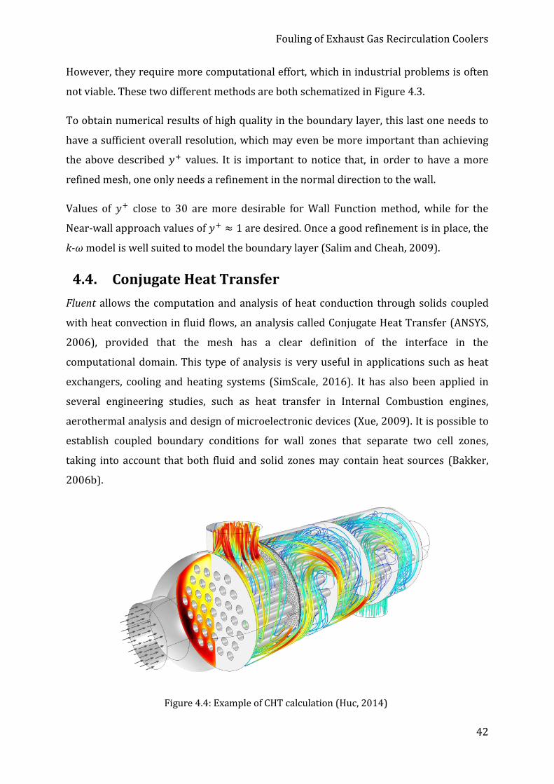
Fouling of Exhaust Gas Recirculation Coolers
42
However, they require more computational effort, which in industrial problems is often
not viable. These two different methods are both schematized in Figure 4.3.
To obtain numerical results of high quality in the boundary layer, this last one needs to
have a sufficient overall resolution, which may even be more important than achieving
the above described 𝑦+ values. It is important to notice that, in order to have a more
refined mesh, one only needs a refinement in the normal direction to the wall.
Values of 𝑦+ close to 30 are more desirable for Wall Function method, while for the
Near-wall approach values of 𝑦+ ≈ 1 are desired. Once a good refinement is in place, the
k-ω model is well suited to model the boundary layer (Salim and Cheah, 2009).
4.4. Conjugate Heat Transfer
Fluent allows the computation and analysis of heat conduction through solids coupled
with heat convection in fluid flows, an analysis called Conjugate Heat Transfer (ANSYS,
2006), provided that the mesh has a clear definition of the interface in the
computational domain. This type of analysis is very useful in applications such as heat
exchangers, cooling and heating systems (SimScale, 2016). It has also been applied in
several engineering studies, such as heat transfer in Internal Combustion engines,
aerothermal analysis and design of microelectronic devices (Xue, 2009). It is possible to
establish coupled boundary conditions for wall zones that separate two cell zones,
taking into account that both fluid and solid zones may contain heat sources (Bakker,
2006b).
Figure 4.4: Example of CHT calculation (Huc, 2014)

Fouling of Exhaust Gas Recirculation Coolers
43
In this kind of analysis, the Navier-Stokes equations are solved for the fluid domain,
whereas as the heat conduction is solved in the solid domain; the temperature and heat
transfer coefficients at the interface between the two domains will be determined by a
local energy balance, at every cell. It is of extreme importance to define correctly the
boundary conditions – existing heat sources and conditions of the flow, such as effects of
buoyancy, natural or mechanic convection, laminar or turbulent flow, etc. – and make
sure the meshing on the interface between the two domains is properly defined.
The interface boundary conditions require the same heat flux and temperature for both
the fluid and the solid at all boundary points, on each grid node along the interface. The
information on each neighboring node (from both sides) is saved and updated at every
iterative step, for all the variables (temperature, pressure, etc) (Xue, 2009).
𝑘𝑓𝑙𝑢𝑖𝑑
𝜕𝑇
𝜕𝑛|𝑓𝑙𝑢𝑖𝑑
= 𝑘𝑠𝑜𝑙𝑖𝑑
𝜕𝑇
𝜕𝑛|𝑠𝑜𝑙𝑖𝑑
( 4.8 )
However, regarding this dissertation, the interest lies only on the results for the fluid
side, as the objective is to assess the fouling effect on the gas-side of the cooler.
4.5. CFD Coupling using UDF
User defined functions (UDF) are programmed routines in C language that allow to
customize Fluent, enhancing its modelling capabilities. It permits the tailoring of the CFD
for special applications, which otherwise would not be obtainable with standard Fluent
interface. (Yan, 2011, ANSYS, 2016a)
Regarding this dissertation, several UDFs were supplied by Atlanting GmbH in order to
allow the simulation of the EGR Cooler studied at DEUTZ AG, enabling the gathering of
results concerning deposit thickness, heat fluxes, condensation rates, etc. inside the
cooler. The UDFs are identified by a “.c” extension and a header file designated by “.h”
that allows to direct and include the function in the compilation process.
The simulation process is divided into two stages:
• CHT analysis – basic Fluent analysis;
𝑇𝑓𝑙𝑢𝑖𝑑 = 𝑇𝑠𝑜𝑙𝑖𝑑 ( 4.7 )

Fouling of Exhaust Gas Recirculation Coolers
44
• Fouling analysis – running of the UDFs.
The UDFs are initially introduced (but not hooked) in Fluent software when all the
boundary conditions are set for the CHT calculation. They should be compiled and not
interpreted. Then the file is saved and again reopened, for the header file that associates
the user defined memories names to load the renamed fouling routines. This way the
fouling model will be able to run properly.
The simulation is then started until one obtains converged values (generally around
1000 iterations are necessary). This step is purely the steady state CHT analysis, without
the fouling; that is, only the cooling performance of the (clean) cooler is analysed – that
is, the heat transferred between gas and coolant -, along with the evolution of the
exhaust gas flowing within (pressure drop, temperature difference, etc.), with basic
Fluent settings. This stage is of extreme importance as the calculated flow, the turbulent
behavior and temperature fields will be used as input information for the determination
of the fouling analysis. However, in this initial simulation for CHT analysis, the option for
layer conduction model must be already activated (at the gas side of the cooler wall) and
with the limit value defined, as it is essential for the fouling model. If it is not initially
activated, the solution will lose the values of the CHT analysis when starting the fouling
model.
The value defined for the maximum layer thickness in the model depends on the cooler.
It was actually fixed (but never reached) 1.3 mm, as a recommendation from the
routines supplier, and it cannot be later changed in the fouling analysis. Also, the
characteristics of the deposits need to be inserted as a new solid material, with the
following values:
Property Value
Density [kg/m3] 17
Specific heat capacity [J/(kg K)] 100
Thermal Conductivity [W/(m K)] 10
Table 4.1 – Property values of pure soot for the deposits
However, the value that has a bigger influence is the thermal conductivity, which is
chosen to make the effect on heat transfer negligible for the CHT analysis.

Fouling of Exhaust Gas Recirculation Coolers
45
This stage of simulation is run with the turbulence model SST k-ω model. Residual
convergence should be turned off and the actual convergence should be assessed based
on the values obtained.
When starting the fouling analysis, three steps must be executed:
• Hooking the UDFs;
• Turning off the unnecessary equations;
• Changing the dependence of the deposits’ thermal conductivity.
Thoroughly explained, after assessing the CHT results, it is necessary to hook the UDFs
to Fluent’s interface, i.e. to activate them. This simulation stage is only about evaluating
the temperature evolution inside the cooler and in the exhaust gas due to the soot
deposit layer, and the final state of equilibrium in the deposited layer. Consequently, in
the menu Solving ⟶ Solution Controls ⟶ Equations the equations for Flow and
Turbulence ought to be disabled, only remaining the Energy equation enabled to
proceed with the heat transfer calculation. The flow no longer plays a role in the fouling
results; the only goal is to determine the heat conduction. As in this stage the values of
the layer will change according to the operating conditions and along the iteration
process, different values will be obtained for its thermal conductivity. Therefore, this
property of the deposits (solid material) ought to be changed in the Fluent’s settings
from constant to user-defined. From now on, this value with differ according to the
boundary conditions introduced by the UDFs.
In the running of the C-routines, two conditions are assumed by them for deposit
calculation:
• The walls are on fluid side and connected to solid;
• The layer thickness activated in the shell conduction model is mandatorily > 0.
Depending on the local boundary conditions, the deposition and removal mechanisms
are calculated until they come to a balance, i.e. until they reach a state of equilibrium and
there is no longer a variation of the results. During this work, only a steady state solution
was sought out, as the routines used provided only the results after reaching a steady
state, that is, the values obtained are not time dependent. This is valid both for the
Conjugate Heat Transfer (CHT) and the Fouling solutions.

Fouling of Exhaust Gas Recirculation Coolers
46
4.6. Errors in CFD Calculations
In CFD analysis (and every other numerical analysis) it is important to keep in mind that
the numerical results are always approximate, because errors may arise from several
sources, and it is not possible to eliminate them all. Therefore, the difference between
reality and computed results lies in simple reasons, such as the following:
• The differential equation may contain approximations, to simplify and make the
calculations possible (considering inviscid flow, irrotational flow, etc.);
• Approximated numerical simulations are based on a discretization process;
• When solving the equations for each discretized domain, iteration processes are
used, which also comes with errors as only running them for an infinite amount
of time, would the exact solution be reached.
The visualization of the numerical solutions through the display of vectors, contours, etc.
that describe the flows is a powerful tool and helps to better understand and have a 3D
view of the flow. However, one needs to be very careful using these methods of post-
processing the information, as many times the errors are not perceptible. The solution
may look good but simultaneously be quantitatively erroneous, and not correspond to
the actual values, boundary conditions, etc. (Ferziger and Peric, 2001). Residuals are the
error magnitudes for the equations as the iterations proceed. They measure the local
imbalance of a conserved variable in each control volume. They include the following
governing equations:
- Navier-Stokes momentum equations;
- Continuity equations (for mass conservation);
- Energy equations (for heat transfer);
- Turbulence model equations.
The objective of running a very high number of iterations (usually > 1000) is to make
the solution converge: that means the errors get smaller and smaller, the equation
values change ever less.
Regarding heat transfer calculations usually a deep convergence is required: the scale
residuals should be of the order of 1e-06 and even lower (Bakker, 2006b).

Fouling of Exhaust Gas Recirculation Coolers
47
5. Method – Model Validation As main objective of this work, a few studies were used as source for validation of the
routines supplied for this dissertation. Thence, a basic geometry is described in these
documents, where several test bench experiments were performed according to it,
obtaining values to be compared with the simulation analysis performed in this
dissertation.
5.1. Geometry
Figure 5.1 depicts the geometry of the cooler used by Völk and Hörnig (2011; 2012) in
their study and measurements. It has a double tube construction (concentric tubes) and
the flows of the exhaust gas and the cooling fluid (water) run in opposite directions
(Völk, 2014).
However, it must be stated that the scheme contains an incorrect value: the total length
of the cooler cannot be 290 mm, as 225 plus 65 mm already performs the 290 mm.
Therefore, it will be assumed that the outlet part of the cooler also measures 65 mm.
80
Figure 5.1: Layout of the cooler design for field tests used by Völk and Hörnig (2012)
Fouling of Exhaust Gas Recirculation Coolers
48
The cooler tube is made of aluminium, with a length of 160 mm, outer diameter of
12mm and wall thickness of 1 mm (Hörnig, 2012). The control volume used for the
simulations performed in this dissertation is defined by the blue rectangle, that is,
specifically just the cooler tube, excluding the inlet and outlet funnels.
The entrance geometry plays a big role in the fouling occurrence, as sudden changes in
geometry are very likely to induce fouling by impaction or interception of soot particles.
Consequently, for legitimate values to be obtained with this geometry, the entrance was
designed based on previous tests on EGR coolers, with the goal of minimizing the fouling
effect (Hörnig et al., 2011).
The equations of mass and energy conservation of the flow inside the cooler are
simplified, as the following assumptions are made:
• Coolant temperature is constant and corresponds to the wall temperature (the
water flow is not considered for this dissertation – and for that matter, nor in
the sources used);
• Soot properties do not vary with deposit thickness or temperature.
As previously stated, the water-side flow was not considered in the study of Völk and
Hörnig (2011, 2012). The water flow was setup in such conditions that the boundary
condition defined at the outer wall of the inner tube was of constant temperature: the
water flow was so high that the difference between the water temperature at the inlet
and outlet is practically irrelevant, thus eliminating the need to study this flow.
With this geometry, two different test benches were set by Völk and Hörnig (2011) to
perform the measurements. They are described in sections 5.6 and 5.7.
5.2. Mesh Characteristics and Influence
It is important to focus on the importance of the definition of the mesh used to perform
the simulations, as it has a great impact on the final results. A coarse grid will cause poor
spatial resolution of the gas phase results and, consequently, lead to a poor prediction of
the interactions between gas and liquid phases (Xue, 2009). A refined mesh, with equal
cell-wall distance along the entire radial cross-section of the tube was used, for a good
accuracy of the simulations.

Fouling of Exhaust Gas Recirculation Coolers
49
The mesh was developed and after the values of 𝑦+ were tested to see if they fitted the
recommended values for the near-wall treatment. One can only know the values of 𝑦+
after running an initial simulation, since this value depends on the local fluid velocity
and on the mesh; therefore, it is not possible to know it beforehand. The zoom on the
mesh depicted in Figure 5.3 shows clearly the equal wall-cell distance, along the whole
radial cross-section.
Figure 5.3 - Zoom-in on the final mesh used for the inside of the tube, 1/4 of the radial cross-section displayed
Figure 5.2 - Screenshot of the mesh used in Fluent for the chosen cooler geometry

Fouling of Exhaust Gas Recirculation Coolers
50
This mesh is extremely refined and uniform near the inner wall of the cooler, at the
interface with the gas, where the deposit layer will set in, as it can be seen in Figure 5.3.
5.3. Exhaust Gas Composition
The simulations performed in this dissertation used several properties indicated by the
supplier of the C-routines, Atlanting GmbH. The exhaust gas composition follows an
ideal gas behavior. However, some properties such as the thermal conductivity, specific
heat capacity and thermal conductivity are temperature dependent values, hence its
introduction in Fluent as a piece-wise linear evolution, with the extreme points at 100 °C
and 400 °C. The values presented in the next tables match the ones for ideal gas air, as
mentioned. The properties of the cooler side are not important, even though one knows
water is the fluid used. It is, nonetheless, not contemplated in the simulations in the
scope of this thesis, as previously mentioned. The only needed parameter is the
temperature on the water side, which will be considered constant temperature as a
boundary condition.
Temperature
[°C]
Thermal Conductivity
[W/(m K)]
Specific heat capacity
[J/(kg K)]
Dynamic Viscosity
[kg/(m s)]
100 0.03139 1012 2.194E-05
400 0.04996 1069 3.335E-05
Table 5.1 - Description of the values adopted for the thermal conductivity, specific heat capacity and dynamic viscosity of the exhaust gas for a piece-wise linear
evolution
5.4. Sulphur Concentration
As it can be seen on Table 5.2 the sulfur content is described in concentration of H2SO4.
Therefore, a conversion needs to be done in order to have the value for the SO2 content,
as this is the one to be inserted as input in the routines.
During the combustion, most of the sulphur is transformed into SO2, from which around
2% will be oxidized to SO3. Then the emerging SO3 quickly reacts with the water vapor
existing in the exhaust gas, thus forming H2SO4. This can reinforce the particle
deposition, through the condensation of the sulfuric acid, when the dew point of 112 °C –
120 °C is reached in the exhaust gas flow through the cooler (Völk, 2014).

Fouling of Exhaust Gas Recirculation Coolers
51
According to Atlanting (2016), the conversion relationship between SO2 and H2SO4 used
in their code is:
𝐻2𝑆𝑂4𝑐𝑜𝑛𝑡𝑒𝑛𝑡
= 𝑆𝑂2𝑐𝑜𝑛𝑡𝑒𝑛𝑡×0.03 ( 5.1 )
Nowadays, sulphur plays an ever-smaller role in combustion and gas emissions. Ever
since 2009, the European Union has set the sulphur level to a maximum of 10 ppm (as a
mass ratio) in diesel fuel for passenger vehicles and light commercial vehicles. For non-
road vehicles and machines the maximum value was set on 1000 ppm until the end of
2011, when the study used as source was produced (Völk and Hörnig, 2011); since then
and until the present this value is also at a maximum of 10 ppm (Völk, 2014). The 1000
ppm content of sulphur corresponds to a 3.6 ppm amount of H2SO4 in the gas phase.
For the motor test bench, the value adopted by Völk and Hörnig (2011) was 18 ppm of
sulphur in the diesel fuel, which coincides with 0.065 ppm of H2SO4 in the gas phase,
according to the existing proportion.
In the following table are depicted the values for the conversions for both motor and
model test bench used sulphur contents, according to the proportion stated and to the
conversion relationship used by Atlanting (2016). These concentrations in ppm refer to
a mass ratio of sulphur per mass of fuel.
Table 5.2 - Values of sulphur and respective conversions to SO2 and H2SO4 used in both test benches
Fuel Exhaust gas
Sulphur [ppm] SO2 [ppm] H2SO4 [ppm]
1000 120 3.6
18 2.17 0.065
55.6 6.67 0.2
2777.8 333.3 10

Fouling of Exhaust Gas Recirculation Coolers
52
5.5. Soot Particles in Exhaust Gas
Soot is an extremely variable and changeable component. Its properties depend on
several factors in the combustion cycle, such as: air-fuel ratio, oxygen content in the
intake air, fuel composition, the mixture between air and fuel, loading charge, EGR rate
and cylinder temperature (Hörnig, 2012). The particle size distribution is a critical
factor for the growth rate and different constitutions of particulate fouling, as during the
combustion not only coarse particles emerge but also aerosols (microscopic particles)
(Abd-Elhady et al., 2011); therefore, particle concentration distribution was a
thoroughly studied and meticulously analysed topic throughout the production of this
dissertation.
The graphic displayed in Figure 5.4 is a continuous lognormal distribution curve for the
soot emitted both on the motor test bench, as on the model test bench. As a continuous
distribution, the total area under each curve corresponds to the total number of
particles emitted by each diesel source, according to the integral (Park et al., 2014):
∫d𝑛
d𝑑d𝑑 = 𝑛 ( 5.2 )
The unit depicted on the ordinate is a differential particle number concentration, that is:
the particle number is normalized by range of particle diameter of the interval, which
shows that the curve works in particle size (diameter) intervals. For this reason, we
cannot determine the concentration of particle number for one specific particle
diameter, but instead for a class of several diameters.
As the number of particles is the dependent variable it is described as a number
distribution; if dN is the number of particles in a certain size interval from 𝑑𝑝 to 𝑑𝑝 +
d𝑑𝑝, then the number distribution function 𝑛(𝑑𝑝) can be described as (Kulkarni et al.,
2011):
𝑑𝑁 = 𝑛(𝑑𝑝)d𝑑𝑝 ( 5.3 )

Fouling of Exhaust Gas Recirculation Coolers
53
and since it typically ranges over several orders of magnitude, it is useful to describe the
size interval as d log(𝑑𝑝), and the size distribution will transform to:
𝑑𝑁 = 𝑛(log𝑑𝑝)d log (𝑑𝑝) ( 5.4 )
In addition to this, the particle size distribution can be viewed in two different ways: as
frequency of distribution of the number of particles, such as displayed in Figure 5.4 and
the exemplary curve for the function 𝑞𝑟(𝑥) in Figure 5.5, or as the cumulative
distribution, corresponding to the curve of 𝑄𝑟(𝑥) (Stieß, 2008). They both contain the
same information but the differential plot gives a better presentation of the distribution
shape, and any effect of bias is not propagated throughout the entire size plot, as it
happens with the cumulative plot. However, this last one provides a better estimate of
the median diameter of the aerosol. The cumulative distribution is a percentage
distribution of the variable displayed, which indicates always its value below a certain x
value, between 𝑥𝑚𝑖𝑛 and 𝑥𝑚𝑎𝑥 . It can be described by the following equation:
𝑄𝑟(𝑥𝑖) =
𝑝𝑎𝑟𝑡𝑖𝑎𝑙 𝑎𝑚𝑜𝑢𝑛𝑡 𝑜𝑓 𝑣𝑎𝑟𝑖𝑎𝑏𝑙𝑒 𝑥𝑚𝑖𝑛 …𝑥𝑖
𝑡𝑜𝑡𝑎𝑙 𝑎𝑚𝑜𝑢𝑛𝑡 𝑜𝑓 𝑣𝑎𝑟𝑖𝑎𝑏𝑙𝑒 𝑥𝑚𝑖𝑛 …𝑥𝑚𝑎𝑥 ( 5.5 )
The curve of 𝑄𝑟(𝑥) cannot decrease because the proportion of the quantity below a
particle size 𝑥𝑏 cannot be lower as the one below 𝑥𝑎, if 𝑥𝑎 < 𝑥𝑏 , since this curve
Electrical mobility diameter dm [mm]
Par
ticl
e n
um
ber
con
cen
trat
ion
Figure 5.4 - Distribution of the concentration of the number of particles for the different types of soot emitted, per mobility diameter (Völk and Hörnig, 2011)

Fouling of Exhaust Gas Recirculation Coolers
54
represents the cumulative values of the frequency distribution curve (Stieß, 2008). The
following is also to be noted:
• for 𝑥 ≤ 𝑥𝑚𝑖𝑛, then 𝑄𝑟(𝑥) = 0;
• for 𝑥 > 𝑥𝑚𝑎𝑥, then 𝑄𝑟(𝑥) = 1.
On the other hand, the frequency distribution shows the total amount of the variable
inserted in one specific interval of sizes, a specific class, and can be defined by (Stieß,
2008):
𝑞𝑟(𝑥𝑖) =
𝑎𝑚𝑜𝑢𝑛𝑡 𝑜𝑓 𝑣𝑎𝑟𝑖𝑎𝑏𝑙𝑒 𝑥𝑖−1 …𝑥𝑖
𝑡𝑜𝑡𝑎𝑙 𝑎𝑚𝑜𝑢𝑛𝑡 𝑜𝑓 𝑣𝑎𝑟𝑖𝑎𝑏𝑙𝑒 ∙ 𝑤𝑖𝑑𝑡ℎ 𝑜𝑓 𝑡ℎ𝑒 𝑖𝑛𝑡𝑒𝑟𝑣𝑎𝑙 ( 5.6 )
The frequency distribution can be obtained from the cumulative distribution through
the following relationship:
𝑞𝑟,𝑖 =
𝑄𝑟(𝑥𝑖) − 𝑄𝑟(𝑥𝑖−1)
∆𝑥𝑖=
∆𝑄𝑟,𝑖
∆𝑥𝑖 ( 5.7 )
Thus, sustaining the differential:
𝑞𝑟(𝑥) =
𝑑𝑄𝑟(𝑥)
𝑑𝑥 ( 5.8 )
Finally, it is possible to conclude that:
∫ 𝑞𝑟(𝑥)𝑑𝑥 =
𝑥𝑚𝑎𝑥
𝑥𝑚𝑖𝑛
𝑄𝑟(𝑥𝑚𝑎𝑥) = 1 ( 5.9 )
Figure 5.5 - Frequency and cumulative distribution of a normal distribution (Stieß, 2008)

Fouling of Exhaust Gas Recirculation Coolers
55
From the equations above the following ought to be highlighted:
• for 𝑥 ≤ 𝑥𝑚𝑖𝑛, then 𝑞𝑟(𝑥) = 0;
• for 𝑥 ≥ 𝑥𝑚𝑎𝑥, then 𝑞𝑟(𝑥) = 0;
• for 𝑥 = 𝑥𝐼𝑃, at the inflection point IP of the function 𝑄𝑟(𝑥), then 𝑞𝑟(𝑥) has a
maximum value.
This relationship described verifies for every type of particle variable depicted on the y-
axis, such as: number, length, area, volume and mass. Particle number is the variable
type addressed in this chapter and it is the only one of interest for the scope of this
dissertation and simulations.
In order to assess the influence of the particle size distribution in the soot deposition
along the cooler, the mass fractions of several particle classes were calculated. As
indicated by the routine supplier, five different particle classes should be introduced as
input parameters in the UDF code in order to perform the simulation. Therefore, the
mass fractions were calculated both for the Motor test bench, as for the Model test
bench, respectively: the curve for 2000 1/min@5bar and the Flammruß (flame soot)
curve in Figure 5.4. However, the cumulative curve allows the acquirement of a better
feeling of the distribution of the particles, reason why the curves of Figure 5.4 were
integrated in order to obtain their respective cumulative displays, and regarding the
particles mass. They provided a clearer view of the weight of the different particle
diameters in the total soot mass and sped up the determination of the mass fractions for
each source, and for the different particle size classes, whose influence will be analysed
in further chapters. This was achieved with the use of 20 points in both the diesel and
flame soot curves, allowing the obtaining of a smoother and more precise curve, than if
using a smaller number of points. The curves in the following graphic were obtained by
converting the distribution curve from Figure 5.4 in a finite number of zones (histogram
view of the distribution): whose middle values correspond to the 20 points. Thus, 20
different columns were drawn, as the example sketched in Figure 5.6.
In every column, a medium diameter (corresponding to the chosen point) is defined as:
𝐷𝑚𝑒𝑑 =
𝐷𝑖 + 𝐷𝑖+1
2 ( 5.10 )

Fouling of Exhaust Gas Recirculation Coolers
56
based on the extreme diameters of every column. The value of particle number
concentration corresponding to that medium diameter is then read on the y-axis.
Therefore, the area of one column/rectangle will be given by:
𝐴𝑟𝑒𝑎1𝑐𝑜𝑙𝑢𝑚𝑛 = [
# 𝑝𝑎𝑟𝑡𝑖𝑐𝑙𝑒𝑠
𝐷 ∙ 𝑣𝑜𝑙𝑢𝑚𝑒] ∙ [𝐷𝑖+1 − 𝐷𝑖] ( 5.11 )
and the approximate total area under the curve of particle number concentration is
given by the sum of the areas of the columns, since the unit of the values read on the y-
axis of the graphic are [#/(diameter×m3)]. As it is a continuous distribution, the number
concentration is proportional to the area of each column. Consequently, the mass of
particles (per unit volume) associated with one specific medium diameter is given by:
𝑚1𝑐𝑙𝑎𝑠𝑠 =
# 𝑝𝑎𝑟𝑡𝑖𝑐𝑙𝑒𝑠
𝐷 ∙ 𝑣𝑜𝑙𝑢𝑚𝑒∙ [𝐷𝑖+1 − 𝐷𝑖] ∙ 𝑚1𝑝𝑎𝑟𝑡𝑖𝑐𝑙𝑒 ( 5.12 )
The mass of one diesel particle was obtained by the equation (5.12) recommended by
Cambustion (2009) for size relationship with mass:
𝑚1𝑝𝑎𝑟𝑡𝑖𝑐𝑙𝑒 [𝜇𝑔] = 2.20 ∗ 10−15 ∙ 𝐷𝑝
2.65 [𝑛𝑚] ( 5.13 )
which was derived from the particle mass measurement with DMS spectrometers.
Figure 5.6 - Scheme of the calculation of the area of each of the classes chosen to obtain the cumulative mass particle distribution

Fouling of Exhaust Gas Recirculation Coolers
57
Finally, the mass fractions for one particular class with the respective medium diameter
are given by:
Above in Figure 5.7, the two cumulative mass fractions curves for both test bench soot
types are obtained, through the process explained. An approximation with a 3rd degree
polynomial and a Fourier transform was pursued, in order to determine the mass
fraction values for the diameter classes chosen for the model test bench. They are both
fairly precise in adjusting the curve with the original mass fraction values, as one can see
in Figure 5.8.
Hence, the 3rd degree polynomial curve was chosen for this effect. Through the use of the
equation that defines this polynomial, the values for every extreme point of each of the
five classes are introduced in the equation and the respective mass fractions are
obtained.
To obtain the mass fractions for the five chosen medium diameters, one simply has to
subtract the lower value of the class to the higher value of the class, for instance: to
determine the mass fraction matching the diameter of 125 nm one needs to subtract the
𝑚𝑎𝑠𝑠 𝑓𝑟𝑎𝑐𝑡𝑖𝑜𝑛1𝑐𝑙𝑎𝑠𝑠 =
𝑚𝑎𝑠𝑠 𝑜𝑓 𝑜𝑛𝑒 𝑐𝑙𝑎𝑠𝑠
𝑚𝑎𝑠𝑠 𝑜𝑓 𝑎𝑙𝑙 𝑐𝑙𝑎𝑠𝑠𝑒𝑠 ( 5.14 )
Figure 5.7 - Cumulative Mass Fraction Curves for Diesel and Flame Soot

Fouling of Exhaust Gas Recirculation Coolers
58
mass fraction from 100 nm to the one from 150 nm. The final mass fractions for both
model and motor test bench are displayed in Tables 5.3 and 5.4.
Table 5.3 - Mass fractions associated to flame soot – model test bench - to be used as input for
the UDFs
Regarding the motor test bench also two curves were used to approximate the original
cumulative mass fractions curve. However, in this one, one can conclude from Figure 5.9
that the Fourier transform approximates better the original curve than the polynomial
case does.
Class Medium Diameter
[nm] Mass Fraction
50 0.04
125 0.11
175 0.15
275 0.51
400 0.19
Figure 5.8 - Approximation curves to the cumulative mass fractions of the model test bench

Fouling of Exhaust Gas Recirculation Coolers
59
Class Medium Diameter
[nm] Mass Fraction
50 0.06
125 0.15
175 0.18
275 0.45
400 0.16
Table 5.4 - Mass fractions associated to diesel soot from motor test bench to be used as input for the UDF
Figure 5.9 - Approximation curves to the cumulative mass fractions of the motor test bench

Fouling of Exhaust Gas Recirculation Coolers
60
5.6. Motor Test Bench
This test bench consisted on using the exhaust gas from a real diesel engine and linking
it to the simple cooler geometry displayed above, where part of the exhaust gas can be
recirculated. The exhaust gas provided for this test bench assessment was procured
from a turbocharged BMW M57D30 TÜ2 diesel engine, in three different load operating
points: 1000 min-1 at 1 bar, 1500 min-1 at 3 bar and 2000 min-1 at 5 bar (mean effective
pressure 𝑝𝑚𝑒). For the simulations performed about the motor test bench, however, only
the highest load point was used, as it can be seen ahead in Figure 5.5., this is the point
with highest particle concentrations; for this reason, Völk and Hörnig (2011) chose it to
draw conclusions in their measurements.
The other two lower operating points generated very low deposition values (due to low
particle concentration) in order to allow a valid analysis of the fouling effect. As the
exhaust gas characteristics are fully defined for this engine, it is not possible to make
singular changes in its composition, such as, for example, increasing the particle or HC-
concentration, which would raise the propensity for soot deposition. For the chosen
operating point, three different EGR-Rates were used to perform the measurements.
Their values and corresponding exhaust gas data are displayed in Table 5.5:
EGR-Rate [kg/h] 4.5 9 15
Re [-] 5600 11000 16000
HC [ppm] 350-450 350-450 350-450
Soot mass flow [mg/h] 91.15 210.01 575.30
Table 5.5 - Exhaust gas data for the three different EGR-Rates used in model test bench by Völk and Hörnig (2011)
In this test bench, two different cases were picked from Völk and Hörnig (2011) to use
as basis for comparison with the simulations performed, from here on described as Test
Case 1 and Test Case 2. Their measurement results are described ahead in Chapter 7.
The concentrations in ppm refer to a mass ratio.

Fouling of Exhaust Gas Recirculation Coolers
61
Test Case 1 Test Case 2
Variable Description Value Value
Exhaust gas mass flow [kg/s] 9 15
Exhaust gas inlet temperature [°C] 300 380
Soot mass flow [mg/h] 210.01 575.3
Cooling water temperature [°C] 20, 40, 60, 80 20, 80
HC concentration [ppm] 350 - 450 350 - 450
SO2 concentration [ppm] 2.17 2.17
H2O concentration [kg/kg] 2% - 11% 2% - 11%
Table 5.6 - Description of the main input parameters for Test Cases 1 and 2 of motor test bench
5.7. Model Test Bench
In pursuance of isolating the different influences on the particle deposition in the motor
test bench, a new test bench was developed, where the exhaust aerosol constitution was
previously modelled, that is, it is fully customizable. Here follows a scheme of the setup
used to produce this modelled exhaust gas.
The model aerosol used for the model test bench was obtained by first heating dry
particulate free pressurized air up to a desired temperature, reaching values of 450 °C.
Amounts of water, sulphuric acid and diesel fuel were added to the aerosol in values
comparable to real diesel exhaust emissions. HC concentration levels were chosen based
on previous measurements, which places them between 200 and 450 ppm – relatively
high values. Thereafter, soot produced by a flame or diffusion burner is added to the
heated gas (Hörnig et al., 2011).
Figure 5.10 - Schematic setup of the model test bench (adapted) (Völk and Hörnig, 2011)

Fouling of Exhaust Gas Recirculation Coolers
62
In this test bench, different exhaust gas compositions can be created through the
variation in content of: water, adsorption of hydrocarbons and sulphur to the soot
particles. The soot used for this test bench was polydisperse flame soot from a propane
burner with �̇�𝑠𝑜𝑜𝑡 = 45 mg/h, defined by Völk and Hörnig (2011, 2012). Their study
also contemplated another type of soot; it had, however, too low particle concentration
to allow significant deposition that could have a valid analysis, as it can be seen in Figure
5.4 by the name of GfG-Ruß (soot from Graphite radio-aerosol). Furthermore, the soot
source chosen provides a rather high and constant mass flow, crucial for a good fouling
analysis in this test bench. Also, it is important to notice that both modelled types of soot
have a particle size distribution that is comparable the one of real diesel engine soot,
used in motor test bench, as can be verified by the Figure 5.4.
The exhaust gas flow (EGR-Rate) used for this test bench varied from 5 to 15 kg/h but
the one chosen for the simulations was �̇�𝑒𝑥ℎ𝑎𝑢𝑠𝑡 = 5.5 kg/h, which verified for every
operating point described in Table 5.7.
Table 5.7 - Description of the several operating points used at the motor test bench by Völk and Hörnig (2011)
Working
point
𝑇𝑖𝑛
[°C]
𝑇𝑤𝑎𝑡𝑒𝑟
[°C]
𝑇𝑜𝑢𝑡
[°C]
𝑇𝑖𝑛 − 𝑇𝑜𝑢𝑡
[°C]
𝑐𝐻𝐶
[ppm]
𝑐𝐻2𝑂
[%]
𝑐𝐻2𝑆𝑂4
[ppm]
E 300 20 240 60 0 0 0
F 150 20 110 40 430 2 0.2
G 150 80 130 20 430 2 0.2
I 150 20 110 40 430 2 10
J 400 20 320 80 230 0 0
K 400 20 320 80 430 0 0
L 400 20 330 70 0 2 0
M 400 20 290 110 0 5 0
N 400 20 310 90 430 2 0
O 400 20 320 80 430 2 10

Fouling of Exhaust Gas Recirculation Coolers
63
6. Simulation Parameters
Firstly, it will be made an approach to the study referred before, performed by Völk and
Hörnig (2011, 2012), using basic Fluent. Simulations will be made based on some of
their measurements and results obtained both for the motor and model test bench. The
first simulations performed were carried out using the above-mentioned geometry
(Chapter 5). The goal of this dissertation was to validate the routines with the described
model and then study the behavior of a real cooler from DEUTZ AG.
In order to perform the simulations, it is necessary to determine all the inputs for the
UDFs regarding the exhaust gas characteristics. According to the UDF code the following
values in the exhaust gas ought to be pre-established and inserted in the respective
parameter routine:
Table 6.1 - Parameters introduced in the UDFs
Parameter of Exhaust Gas Units
Soot concentration kg/kg
HC concentration ppm
SO2 concentration ppm
Water vapour concentration kg/kg
Soot particle for five diameter classes m
Soot particle mass fraction for five diameter classes -
Soot particle density kg/m3
Soot deposit density kg/m3
Molar fraction of short chain HC -
Mass fraction of SO2 converted to sulfuric acid -

Fouling of Exhaust Gas Recirculation Coolers
64
6.1. Features obtained by the UDFs
The routines used throughout this work at DEUTZ AG were provided by Atlanting GmbH
and they made possible to perform the calculations necessary to do a fouling analysis on
EGR coolers, as the Fluent software does not have such specific features. These routines
control whether the steady state or the maximal possible deposit thickness has been
reached. If the state of equilibrium is achieved, species concentrations do not vary
anymore over the cooler length.
Regarding the exhaust gas composition, all the relevant species for the fouling effect
were considered and contemplated in the User Defined Functions: particulate matter,
H2O, HC and H2SO4. It is important to highlight that the condensation of these species
depends on their respective vapour pressure curves, which are depicted in Figure 6.1.
Also, the particle mass fractions have to be introduced in the code, as calculated for the 5
different size classes in section 5.5.
6.1.1. Deposit Thickness
The maximum allowed deposit layer thickness has to be demarcated when defining the
setup for the CHT solution, and cannot be changed thereafter. The deposit thickness
obtained by the measurements of Völk (2014) in his additional work showed almost no
radial variation, that is, in a cross-section of the tube, the deposit thickness was
somewhat constant, even though the cooler was positioned horizontally during the
Figure 6.1 - Vapor pressure curves for every single species considered for the exhaust gas in the routines (Atlanting, 2016)

Fouling of Exhaust Gas Recirculation Coolers
65
experiments: this indicates a generally radial symmetric development of the deposit
layer along the cooler, as long as high amounts of condensate do not emerge.
Therefore, deposit thickness ought to be determined by an Area-Weighted Average (in
the Surface Integrals reports), in order to provide the averaged value of deposit
thickness in the entire cooler. The local consistency of the deposit layer depends on the
amount of soot and condensate that compose the layer.
Usually higher cooling temperatures lead to a faster attainment of a steady state, as the
fouling is dry and creates, therefore, a thinner ultimate deposit thickness. If the number
of adhesive components present in the exhaust gas is reduced, then so will the values of
the correspondent maximum deposition mass and thickness, as the fouling will be less
sticky (Völk and Hörnig, 2011).
6.1.2. Deposition Rates
The deposition rates concern only the soot deposition, that is, the deposition of the
particles of the five different classes, having nothing to do with the species condensation.
Obtaining these allows the direct determination of the deposition efficiency.
6.1.3. Deposition Efficiency
The deposition efficiency can be determined with Fluent and the routines, despite not
being one of the features obtained by the UDFs. In order to do that it is necessary to
firstly understand the concept of deposition efficiency: it describes how effective the
deposition mechanisms are, which allows taking conclusions regarding the propensity
for fouling to occur under the given circumstances in the EGR cooler. The equation (6.1)
by Völk and Hörnig (2011) describes the deposition efficiency for each particle diameter
through the entire cooler:
휀(𝑑𝑝) =𝑐𝑖𝑛(𝑑𝑝) − 𝑐𝑜𝑢𝑡(𝑑𝑝)
𝑐𝑖𝑛(𝑑𝑝) ( 6.1 )
On the other hand the equation (6.2) by Hörnig et al. (2011) describes the deposition
efficiency of a determined particle size depending on the position in cooler length.
휀𝑛 = 𝑁(𝑥 = 0) − 𝑁(𝑥)
𝑁(𝑥 = 0)∙ 100% ( 6.2 )
Fouling of Exhaust Gas Recirculation Coolers
66
The deposition efficiency matches the percentage of the integral of the five different
deposition rates (from the five diameter classes), in the total amount of soot mass flow
in the initially clean cooler. That is, after the CHT calculations have been performed and
the fouling simulation mode has been activated, with the hooking of the UDFs, the
deposition rates can be determined (Atlanting, 2016).
휀 =𝑆𝑢𝑚 𝑜𝑓 𝑡ℎ𝑒 𝑖𝑛𝑡𝑒𝑔𝑟𝑎𝑙𝑠 𝑜𝑓 𝑡ℎ𝑒 𝑓𝑖𝑣𝑒 𝑑𝑒𝑝𝑜𝑠𝑖𝑡𝑖𝑜𝑛 𝑟𝑎𝑡𝑒𝑠
𝑇𝑜𝑡𝑎𝑙 𝑠𝑜𝑜𝑡 𝑚𝑎𝑠𝑠 𝑓𝑙𝑜𝑤 ( 6.3 )
Because the routines provide the deposition rates in[𝑘𝑔
(𝑚2∙𝑠)], each deposition rate needs
to be read as the integral on the cooler inner surface (wall on the gas side), in order to
obtain the deposition rate in [kg/s]. Then the deposition efficiency can be calculated as
seen on Equation (6.3).
Regarding the Surface Integration available as a Fluent tool, one can read the values of
parameters through different types of reports, such as: Area-weighted average, Integral,
Mass-weighted average, etc. Depending on the parameter one wants to read, some
reports are better suited than others. Regarding the case of the deposition rates, an
Integral Surface Report was chosen, in detriment of the Area-Weighted Average. This
choice is supported by the statement that the integral on a surface is computed by
summing the product of the facet area and the selected field variable facet value. In
simpler words, it means that each cell value for - in this case - the deposition rate is
multiplied by the respective cell area, and then all values are summed, as expressed in
the Equation (6.4) (ANSYS, 2016b):
∫𝜙𝑑𝐴 = ∑𝜙𝑖|𝐴𝑖|
𝑛
𝑖=1
( 6.4 )
Each facet is associated with a cell in the mesh. Therefore, the values of a certain
variable on facets are the same as the cell values for the respective variable.
After a few iterations – here the simulation runs for about six iterations, as the first ones
have high peak values, which are inconsistent and may be the result of numerical errors
– the integral of the five deposition rates can be read as a Surface Integral Report in
Fluent. It must be referred that node values should not be enabled when post-processing

Fouling of Exhaust Gas Recirculation Coolers
67
any surfaces associated with shells (wall, shadow wall, etc.). The layers share nodes at
the edges, and thus the averaging of such nodes is erroneous.
6.1.4. Condensation Rates
The condensation rates are one of the features possible to obtain directly from the
routines. They contemplate the condensation rates for the following species:
hydrocarbons of long and short-chain – respectively C24H46 and C12H26 -, sulphur (SO2)
and water. They are an important indicator for the speed of the deposit formation under
the given operating conditions. The effect of diffusiophoresis calculated in the routines is
neglected if the mass fraction of all condensate forming species is less than 1.0e-14
kg/kg.
One important value that can help understand the impact of the different condensate
forming species is their molecular weight. The values used in the routines are displayed
on Table 6.2:
Species H2O H2SO4 C12H26 C22H46
Molecular weight
[kg/kmol] 18 98 170 310
Table 6.2 - Values of the molecular weight of the condensate forming species used in the routines
6.1.5. Fouling Factor
This parameter indicates the thermal resistance due to the deposit layer. It is
determined by:
𝐹𝑜𝑢𝑙𝑖𝑛𝑔 𝑓𝑎𝑐𝑡𝑜𝑟 =
𝐷𝑒𝑝𝑜𝑠𝑖𝑡 𝑡ℎ𝑖𝑐𝑘𝑛𝑒𝑠𝑠
𝑇ℎ𝑒𝑟𝑚𝑎𝑙 𝑐𝑜𝑛𝑑𝑢𝑐𝑡𝑖𝑣𝑖𝑡𝑦 [
(𝑚2𝐾)
𝑊] ( 6.5 )
6.1.6. Thermal Conductivity
The reduction of the cooling performance due to the fouling effect is determined by the
impact on local thermal conductivity. A lower thermal conductivity worsens the heat
transfer, thus decreasing the ultimate performance of the cooler. This parameter allows
to ascertain the composition of the deposit layer: when there is no condensation of
species, the thermal conductivity of the layer is 0.1 W/(m K), that is, it means that it is
composed by pure soot – therefore, it is the minimal value possible to have. On the other
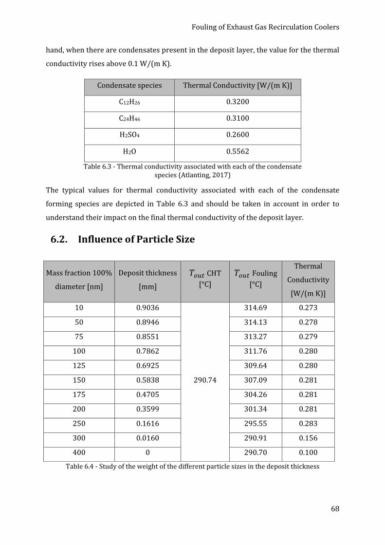
Fouling of Exhaust Gas Recirculation Coolers
68
hand, when there are condensates present in the deposit layer, the value for the thermal
conductivity rises above 0.1 W/(m K).
Condensate species Thermal Conductivity [W/(m K)]
C12H26 0.3200
C24H46 0.3100
H2SO4 0.2600
H2O 0.5562
Table 6.3 - Thermal conductivity associated with each of the condensate species (Atlanting, 2017)
The typical values for thermal conductivity associated with each of the condensate
forming species are depicted in Table 6.3 and should be taken in account in order to
understand their impact on the final thermal conductivity of the deposit layer.
6.2. Influence of Particle Size
Table 6.4 - Study of the weight of the different particle sizes in the deposit thickness
Mass fraction 100%
diameter [nm]
Deposit thickness
[mm]
𝑇𝑜𝑢𝑡 CHT
[°C]
𝑇𝑜𝑢𝑡 Fouling
[°C]
Thermal
Conductivity
[W/(m K)]
10 0.9036
290.74
314.69 0.273
50 0.8946 314.13 0.278
75 0.8551 313.27 0.279
100 0.7862 311.76 0.280
125 0.6925 309.64 0.280
150 0.5838 307.09 0.281
175 0.4705 304.26 0.281
200 0.3599 301.34 0.281
250 0.1616 295.55 0.283
300 0.0160 290.91 0.156
400 0 290.70 0.100

Fouling of Exhaust Gas Recirculation Coolers
69
To understand the weight and impact of the different soot particle sizes in the overall
fouling effect regarding the model test bench, several simulations were performed,
attributing 100% of the particles mass to one particular size class at a time.
As it can be seen in Table 6.4, the smaller particles have a much higher tendency to
deposit than particles of bigger size. Under the present circumstances, particles from
around 400 nm and above no longer deposit at the wall. The deposition forces depend,
therefore, on the size of the particle. As stated in Section 2.4.5 the smaller particles are
more easily driven towards the wall by eddy diffusion than the bigger ones. Also, as seen
by Figure 2.14 from Section 2.7.2, when the velocity of the flow is so high that the
particles at the wall are removed by gas shear stress, this critic velocity that determines
if they are indeed removed or not, increases with the decrease of particle diameter.
Therefore, it means that the bigger particles are much easier to remove. All these factors
explain how the bigger particles may not have any influence in the deposition
phenomenon – in this case, for the model used and in test case K, particles above 400 nm
of diameter do not play anymore a role in the fouling effect.
In the model defined by Atlanting, the size of the particle on the wall will be determined
as the average value of the deposited particles. There it can happen that, for
sensitive/empiric conditions, the deposition stops when the particle is in average too
big.
6.3. Influence of Layer Increment Parameter
The layer increment is a parameter portrayed in the routines which determines the
increase in the build-up of deposit layer in each iteration step. The smaller the value, the
higher the simulation accuracy will be, providing more precise results, however with
higher computational effort and more time; small increments lead to a more extensive
study and calculation of the deposit formation, which takes more time. The default value
used is 0.01 mm. In order to assess the influence of this parameter, an analysis was
conducted using the operating point K with three different layer increment values, for
the five different particle sizes, until the thickness of 0.1 mm was reached. However,
only P3 is displayed as the other particle classes follow the same tendency.
As observed in Figure 6.2, the layer increment value determines how fast the deposition
rate reaches an almost constant value, which induces a linear deposit thickness growth.

Fouling of Exhaust Gas Recirculation Coolers
70
The value cannot exactly be described as constant – as it is further ahead when the
simulation reaches the fouling steady state. The deposition rate will permanently
decrease until it reaches zero at the equilibrium state.
However, it can be considered to achieve a constant value in the first few iterations,
which is the value sought for the deposition rate that will allow to determine the
deposition efficiency. The correct deposition rate value is not exactly the one
corresponding the first iteration because initially the result oscillates considerably,
which might be indicative of numerical errors and may not match the reality, inducing
errors in the determination of the deposition efficiency. Therefore, an empiric analysis
was conducted to determine how many iterations would suffice to describe the initial
deposition efficiency correctly. The deposition rate in the first few iterations assumes
the highest value of deposition rate throughout the whole process, because it occurs
when the cooler is still clean and the heat transfer process is starting to take place, thus
having the highest level of thermophoretic effect and, consequently, a higher deposition
rate.
Figure 6.2 - Graphic displaying the evolution of deposition rate for particle class P3 with three different layer increments

Fouling of Exhaust Gas Recirculation Coolers
71
As it can be seen in Figures 6.3 and 6.4, where the point sought is highlighted in blue, it
reaches a semi-constant value at first, after six iterations of inconsistent values. Then, as
the deposition proceeds, the deposition rate will continuously decrease, until it reaches
zero or, as it is probably the case depicted in Figure 6.4, the removal rates equal the
deposition rates, and the final deposit thickness is obtained, as it no longer increases.
Figure 6.4 - Evolution of the deposition rate of particle class P3 in the first six iterations for operating point K
Dep
osi
tio
n R
ate
[kg/
s]
Figure 6.3 - Evolution of the deposition rate of particle class P3 for operating point K
Dep
osi
tio
n R
ate
[kg/
s]
Fouling of Exhaust Gas Recirculation Coolers
72
Bearing this in mind, the increment used for the execution of the simulations will be
0.001 mm, suggested by the routine supplier, whom advises to choose a smaller
increment value, so that almost no layer is built in each iteration, enabling the
integration of the deposition rate after a few iterations (six as determined by the
analysis of the graphics), once the value has slightly stabilized, thus determining the
most correct deposition efficiency that is possible to obtain.

Fouling of Exhaust Gas Recirculation Coolers
73
7. Simulations and Results
7.1. Simulations – Model Test Bench
The model test bench was the first to be studied. From the operating conditions for this
test bench enunciated previously, five points were chosen to execute the simulations. As
mentioned in section 5.7 the �̇�𝑒𝑥ℎ𝑎𝑢𝑠𝑡 for this test bench is 5.5 kg/h.
Working
point
𝑇𝑖𝑛
[°C]
𝑇𝑤𝑎𝑡𝑒𝑟
[°C]
𝑇𝑜𝑢𝑡
[°C]
𝑇𝑖𝑛 − 𝑇𝑜𝑢𝑡
[°C]
𝑐𝐻𝐶
[ppm]
𝑐𝐻2𝑂
[%]
𝑐𝐻2𝑆𝑂4
[ppm]
E 300 20 240 60 0 0 0
F 150 20 110 40 430 2 0.2
G 150 80 130 20 430 2 0.2
K 400 20 320 80 430 0 0
N 400 20 310 90 430 2 0
Table 7.1- Operating points from the model test bench chosen to perform simulations
From Völk and Hörnig (2011), the only result obtained from the measurements beside
the outlet temperature is the deposition efficiency for every one of the points described
above. Both the deposit thickness and the thermal conductivity are not provided in their
study, but they will be determined in this work, so that one can get a perception of the
relationship between these values and the deposition efficiency.
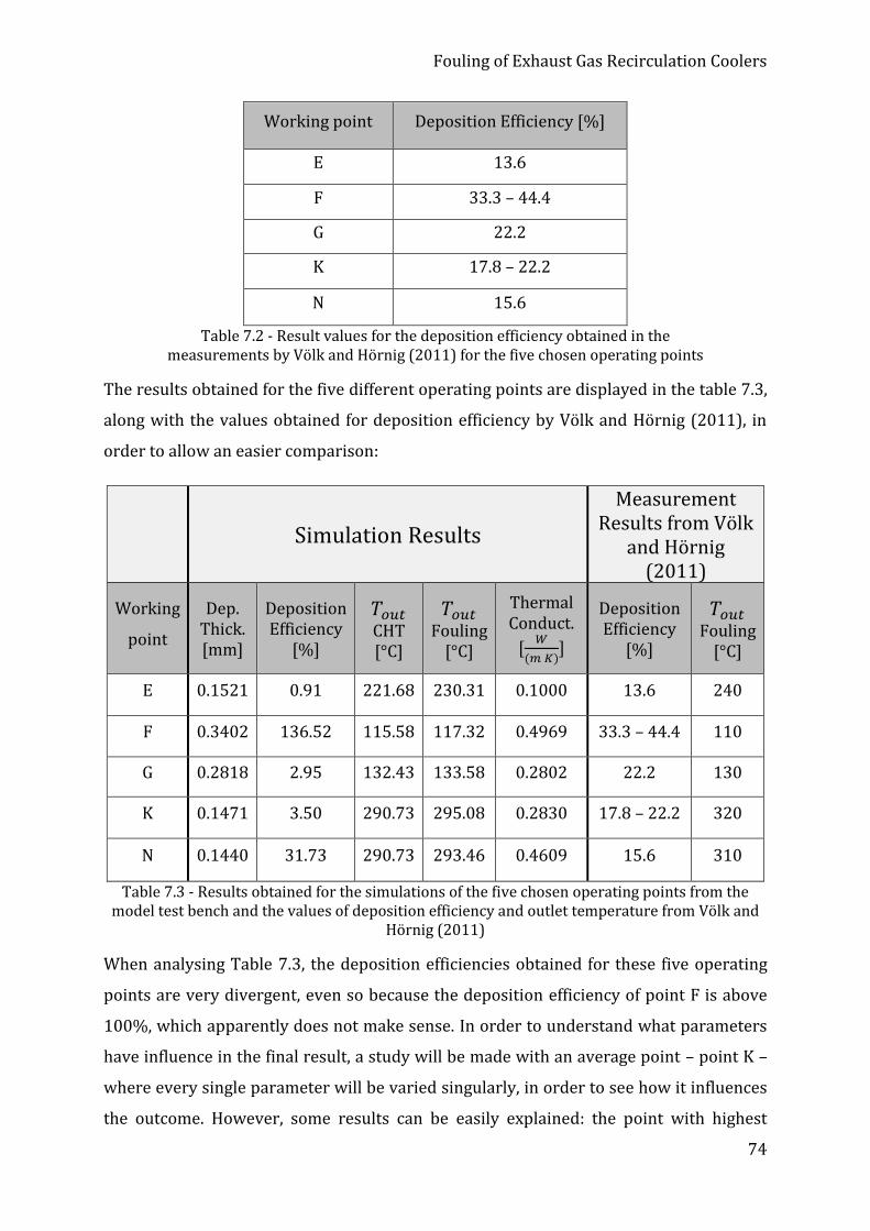
Fouling of Exhaust Gas Recirculation Coolers
74
Working point Deposition Efficiency [%]
E 13.6
F 33.3 – 44.4
G 22.2
K 17.8 – 22.2
N 15.6
Table 7.2 - Result values for the deposition efficiency obtained in the measurements by Völk and Hörnig (2011) for the five chosen operating points
The results obtained for the five different operating points are displayed in the table 7.3,
along with the values obtained for deposition efficiency by Völk and Hörnig (2011), in
order to allow an easier comparison:
Simulation Results
Measurement Results from Völk
and Hörnig (2011)
Working
point
Dep. Thick. [mm]
Deposition Efficiency
[%]
𝑇𝑜𝑢𝑡 CHT [°C]
𝑇𝑜𝑢𝑡 Fouling
[°C]
Thermal Conduct.
[𝑊
(𝑚 𝐾)]
Deposition Efficiency
[%]
𝑇𝑜𝑢𝑡 Fouling
[°C]
E 0.1521 0.91 221.68 230.31 0.1000 13.6 240
F 0.3402 136.52 115.58 117.32 0.4969 33.3 – 44.4 110
G 0.2818 2.95 132.43 133.58 0.2802 22.2 130
K 0.1471 3.50 290.73 295.08 0.2830 17.8 – 22.2 320
N 0.1440 31.73 290.73 293.46 0.4609 15.6 310
Table 7.3 - Results obtained for the simulations of the five chosen operating points from the model test bench and the values of deposition efficiency and outlet temperature from Völk and
Hörnig (2011)
When analysing Table 7.3, the deposition efficiencies obtained for these five operating
points are very divergent, even so because the deposition efficiency of point F is above
100%, which apparently does not make sense. In order to understand what parameters
have influence in the final result, a study will be made with an average point – point K –
where every single parameter will be varied singularly, in order to see how it influences
the outcome. However, some results can be easily explained: the point with highest

Fouling of Exhaust Gas Recirculation Coolers
75
thermal conductivity – point F - shows the highest deposit thickness, which makes sense
since a higher thermal conductivity enables a better heat transfer which, on its own,
generates a greater thermophoretic effect that will lead to a greater deposition of soot
and, therefore, to a thicker deposit. Accordingly, this same point is the one with the
highest deposition efficiency. The operating point E is one extreme point characterized
by pure soot, i.e. there are no condensate forming species, which indicates that the
thermal conductivity of the deposit thickness matches the one of pure soot, 0.1 W/(m K).
Nonetheless, the overall results are unsatisfying, as the values of the deposition
efficiencies do not match the same order of magnitude as the ones provided by Völk and
Hörnig (2011). In the next sections reasons for these discrepancies will be studied.
7.2. Results of Single Effect Variation
This section of Chapter 7 refers to a series of simulations that were performed for a
chosen intermediate point: point K in the model test bench. Several variables were
varied, one at a time, to assess the weight and influence of each one on the final results
of the CFD analysis. For this analysis, no data for comparison is available in the sources.
However, it allows one to have a perception of the influence of each of the variables in
the final results. Such variables were:
• 𝑇𝑤𝑎𝑡𝑒𝑟;
• 𝑇𝑒𝑥ℎ𝑎𝑢𝑠𝑡;
• HC concentration;
• H2O concentration;
• SO2 concentration;
• �̇�𝑒𝑥ℎ𝑎𝑢𝑠𝑡;
• �̇�𝑠𝑜𝑜𝑡.
The original results for point K, without any variable variation are showed on Table 7.4:
Deposit Thickness
[mm]
Deposition Efficiency [%]
𝑇𝑜𝑢𝑡 CHT [°C] 𝑇𝑜𝑢𝑡Fouling
[°C]
Thermal Conductivity
[𝑊
(𝑚 𝐾)]
0.1471 3.500 290.73 295.08 0.2830
Table 7.4 - Original results obtained for the simulations of point K

Fouling of Exhaust Gas Recirculation Coolers
76
7.2.1. Variation of water temperature
The first variation parameter consisted of changing the water temperature (constant
value of temperature on the water-side of the cooler), and keeping the exhaust gas at
400°C and all the species concentration at zero. From Table 7.5 one can conclude that
the tendency observed is that, with increasing water temperature, the deposit thickness
progressively decreases, and so does the deposition efficiency. This is due to a lower
temperature difference which reduces the thermophoretic effect.
Table 7.5 - Results on the variation of the water-side temperature for test case K
𝑇𝑤𝑎𝑡𝑒𝑟 [°C]
Deposit Thickness
[mm]
Deposition Efficiency [%]
𝑇𝑜𝑢𝑡 CHT [°C] 𝑇𝑜𝑢𝑡Fouling
[°C]
Thermal Conductivity
[𝑊
(𝑚 𝐾)]
20 0.1471 3.500 290.73 295.08 0.2830
40 0.1410 3.001 298.08 301.82 0.2818
60 0.1293 2.654 305.06 308.04 0.2844
80 0.1275 2.314 311.56 314.24 0.2862
Figure 7.1 - Evolution of the deposit thickness and deposition efficiency with the variation of water temperature for test case K

Fouling of Exhaust Gas Recirculation Coolers
77
On the other hand, the temperature at the outlet of the cooler progressively increases,
which is coherent with the fact that a higher deposit thickness worsens the heat transfer,
as the thermophoretic effect is endorsed by a higher temperature gradient. This
evidenced by the Figure 7.1, which shows a graphic of the data from Table 7.5.
In addition, the variation of thermal conductivity is very small, as no change is made in
the condensate or soot concentrations, which are the main factors to contribute to its
variation.
7.2.1. Variation of exhaust gas temperature
Regarding the exhaust gas temperature, two different temperatures below and one
above the 400°C from point K were used for the analysis of this parameter, in order to
allow a perception of the evolution of the deposit building when the temperature
gradient is higher and lower to the one of test case K. The results are shown in Table 7.6.
𝑇𝑒𝑥ℎ𝑎𝑢𝑠𝑡 [°C]
𝑇𝑤𝑎𝑡𝑒𝑟 [°C]
Deposit Thickness
[mm]
Deposition Efficiency
[%]
𝑇𝑜𝑢𝑡 CHT [°C]
𝑇𝑜𝑢𝑡 Fouling
[°C]
Thermal Conductivity
[𝑊
(𝑚 𝐾)]
200 20 0.2759 1.394 151.41 154.68 0.3000
80 0.2518 0.749 169.20 170.92 0.3018
300 20 0.2081 2.336 221.61 225.89 0.2917
80 0.1753 1.467 268.09 243.47 0.2944
400 20 0.1471 3.500 290.73 295.08 0.2830
80 0.1275 2.314 311.56 314.24 0.2862
500 20 0.0937 4.774 358.19 361.74 0.2753
80 0.0622 3.300 381.42 382.88 0.2759
Table 7.6 - First results on the variation of the exhaust gas temperature for test case K
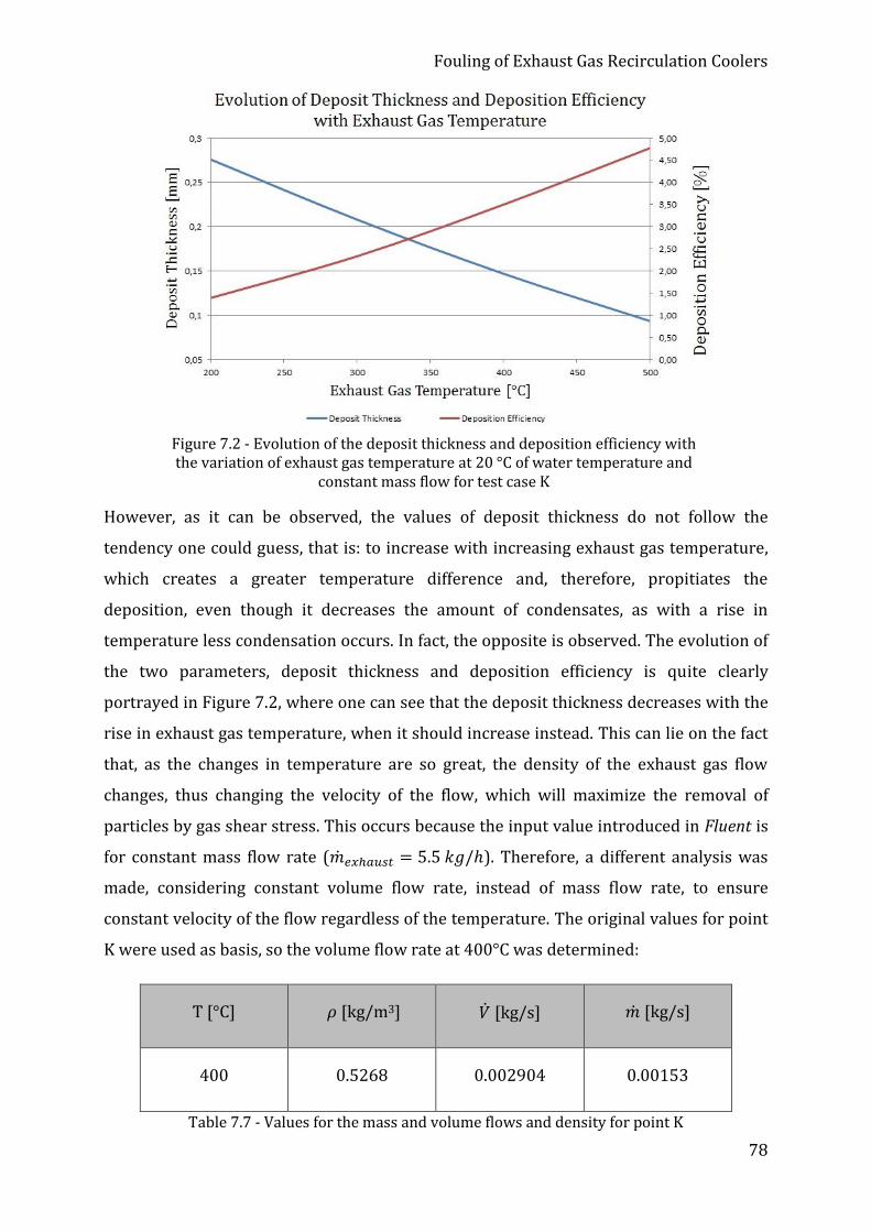
Fouling of Exhaust Gas Recirculation Coolers
78
However, as it can be observed, the values of deposit thickness do not follow the
tendency one could guess, that is: to increase with increasing exhaust gas temperature,
which creates a greater temperature difference and, therefore, propitiates the
deposition, even though it decreases the amount of condensates, as with a rise in
temperature less condensation occurs. In fact, the opposite is observed. The evolution of
the two parameters, deposit thickness and deposition efficiency is quite clearly
portrayed in Figure 7.2, where one can see that the deposit thickness decreases with the
rise in exhaust gas temperature, when it should increase instead. This can lie on the fact
that, as the changes in temperature are so great, the density of the exhaust gas flow
changes, thus changing the velocity of the flow, which will maximize the removal of
particles by gas shear stress. This occurs because the input value introduced in Fluent is
for constant mass flow rate (�̇�𝑒𝑥ℎ𝑎𝑢𝑠𝑡 = 5.5 𝑘𝑔/ℎ). Therefore, a different analysis was
made, considering constant volume flow rate, instead of mass flow rate, to ensure
constant velocity of the flow regardless of the temperature. The original values for point
K were used as basis, so the volume flow rate at 400°C was determined:
T [°C] 𝜌 [kg/m3] �̇� [kg/s] �̇� [kg/s]
400 0.5268 0.002904 0.00153
Table 7.7 - Values for the mass and volume flows and density for point K
Figure 7.2 - Evolution of the deposit thickness and deposition efficiency with the variation of exhaust gas temperature at 20 °C of water temperature and
constant mass flow for test case K

Fouling of Exhaust Gas Recirculation Coolers
79
Using the value of volume flow rate as constant, rather than the mass flow rate, the
following mass flow values for the other temperatures are depicted in Table 7.8.
T [°C] 𝜌 [kg/m3] �̇� [kg/s]
200 0.7487 0.002174
300 0.6184 0.001796
500 0.4589 0.001333
600 0.4066 0.001181
Table 7.8 - Density and mass flow values at constant volume flow from test case K at 400 °C
By the previous table one can verify that, the higher the temperature, the less dense
becomes the flow, which has a direct influence on the mass flow rate (and, per
correlation, on the velocity). Accordingly, the respective mass flows were introduced to
Fluent and the results obtained are displayed in Table 7.9. With these adjustments, it is
clearer the influence the exhaust gas temperature has on the soot layer deposition.
Table 7.9 - Results of the mass flow change pursued regarding the exhaust gas temperature variation for test case K
𝑇𝑒𝑥ℎ𝑎𝑢𝑠𝑡 [°C]
𝑇𝑤𝑎𝑡𝑒𝑟 [°C]
Deposit Thickness
[mm]
Deposition Efficiency
[%]
𝑇𝑜𝑢𝑡 CHT [°C]
𝑇𝑜𝑢𝑡 Fouling [°C]
Thermal Conductivity
[𝑊
(𝑚 𝐾)]
200 20 0.0615 2.649 153.78 154.70 0.2923
80 0.0634 1.249 170.59 171.16 0.2933
300 20 0.1147 3.008 223.30 226.00 0.2869
80 0.0884 1.891 242.36 243.69 0.288
400 20 0.1471 3.500 290.73 295.08 0.2830
80 0.1275 2.314 311.56 314.24 0.2862
500 20 0.1811 3.839 355.91 362.26 0.2796
80 0.1515 2.668 378.23 382.16 0.2831
600 20 0.1860 4.188 421.50 428.45 0.2771
80 0.1750 2.940 441.85 447.25 0.2808

Fouling of Exhaust Gas Recirculation Coolers
80
The higher the temperature, the thicker the deposit layer is, as the deposition is
endorsed by the thermophoresis effect, due to a greater temperature difference.
However the rise in deposit thickness is not too steep because condensation is reduced
with the increase in temperature, thus diminishing the amount of condensates in the
deposit layer.
From Figure 7.3 it is possible to have a better perception of the evolution of the deposit
thickness and deposition efficiency depicted in Table 7.9, for the cases related to 20 °C of
water temperature. After performing the adjustments of the mass flow, it is possible to
conclude that the density of the flow does take a big toll on the final results, because the
two parameters now evolve in the same direction. With increasing exhaust gas
temperature both deposit thickness and deposition efficiency increase, due to a greater
impact of thermophoresis, as previously stated. However, as temperatures of 600 °C are
reached, both variables begin to stagnate; they vary less with the same rise in
temperature. This fact can also be seen in Table 7.8, as the density decrease is steeper
from 300 °C to 500 °C than from 500 °C to 600 °C. This occurs because the air density
(the assumption of air properties for exhaust gas is made, as previously stated) has a
slower increase rate with the temperature rise.
Figure 7.3 - Evolution of the deposit thickness and deposition efficiency with the variation of exhaust gas temperature at 20 °C of water temperature with
respective mass flow variation for test case K

Fouling of Exhaust Gas Recirculation Coolers
81
Now taking a closer look at Table 7.9, one can also observe that with increasing exhaust
gas temperature, the deposition efficiency rises, being also in conformity with the water
side temperature. This corroborates the theoretical background from Section 2.4.1 that
states that, with increasing exhaust gas temperature – and, therefore, increasing
temperature gradient between exhaust gas and the wall -, the thermophoretic effect is
aggravated, thus increasing the amount of soot diverted to the wall which, by itself,
means higher deposition efficiency.
Regarding the relation to the water side temperature, when the 20 °C version is used,
the deposition efficiency is higher than the 80 °C version for the same exhaust gas
temperature. For the deposit thickness, the same tendency between temperatures is
observed, apart from the values for 200 °C, but as the values in question are very small,
one may assume that it might be due to the presence of numerical errors. Regarding the
values of the temperature at the outlet of the cooler, a thicker deposit decreases the heat
transfer and, therefore, the temperature at the exit of the cooler should be higher with
the increase in deposit thickness. This is true for every case. Nonetheless, one needs to
pay attention to the different boundary conditions for the temperatures. Therefore, it is
acceptable that the outlet temperature for 0.1471 mm of deposit is lower than for
0.1275 mm, because the first case is subjected to a temperature difference of 380 °C,
while the latter to one of 320 °C. In addition, one also needs to mind the temperature
without considering the fouling effect, that is, the temperature of the CHT analysis. The
one for the fouling case should always be higher since the deposit is now taken into
account, which indeed happens, as it can be observed; the temperature variations
between CHT and fouling analysis are not too great, but the deposit thickness does not
have very high values as well.
Finally, the performance of the cooler can be assessed by the evolution of the thermal
conductivity which, even though at a low rate, continuously decreases with the rise in
exhaust gas temperature. As stated in Section 2.6, with the increase in exhaust gas
temperature, there is a rise in the deposit thickness due to the fostering of
thermophoresis by a greater temperature difference. This rise in the deposit thickness
makes the surface temperature increase due to the inability of the low thermal
conductivity deposit to transfer the heat from the gas to the metal. The more deposit
there is, the worst becomes the thermal conductivity due to the present of more soot,

Fouling of Exhaust Gas Recirculation Coolers
82
which ultimately prevents the heat transfer, leading to a stabilization of the deposit
thickness - since the temperature at its surface comes near the temperature of flow,
decreasing the thermophoresis. This corroborates the fact that a higher temperature
difference of the fluids in question leads to a worse heat transfer performance, as the
cooler is subjected to the fouling effect that damages the cooler.
7.2.2. Variation of HC concentration
The variation of HC concentration was performed at 𝑇𝑒𝑥ℎ𝑎𝑢𝑠𝑡 = 400 °C, 𝑇𝑤𝑎𝑡𝑒𝑟 = 20 °C,
and both zero concentrations of SO2 and H2O, just like originally in operating point K.
According to Table 7.10 and Figure 7.4 one can observe that the deposit thickness rises
with the increase in HC concentration, which is the expected tendency, as the HC
condensation contributes to the diffusiophoresis effect, bringing more particles towards
the wall. The observed values for the deposit thickness are also in compliance with the
values of thermal conductivity.
Table 7.10 - Results on the single variation of HC concentration for point K
HC [ppm] Deposit
Thickness [mm]
Deposition Efficiency [%]
𝑇𝑜𝑢𝑡 CHT [°C] 𝑇𝑜𝑢𝑡 Fouling
[°C]
Thermal Conductivity [W/ (m K)]
0 0.0930 1.424
290.74
298.09 0.1000
200 0.1394 3.314 295.30 0.2533
300 0.1431 3.405 295.15 0.2697
350 0.1444 3.445 295.10 0.2755
430 0.1471 3.500 295.08 0.2830
450 0.1461 3.520 295.03 0.2842
750 0.1490 3.738 294.93 0.2976
1000 0.1502 3.917 294.90 0.3023
2000 0.1508 4.638 294.83 0.3086

Fouling of Exhaust Gas Recirculation Coolers
83
A bigger amount of HC condensates will lead to an increase in the overall thermal
conductivity - due to the higher thermal conductivity inherent to the hydrocarbons -,
which promotes a thicker deposit layer. It will also have an effect on the deposition
efficiency: a higher amount of condensates brings more particles more easily to the wall,
hence the increase in this value as well.
Through the analysis of Figure 7.4, which depicts the results from Table 7.10, it becomes
clear that, from approximately 700 ppm of concentration, the HC no longer has a
substantial influence on the deposition of soot; however, from around 300 ppm the
change in deposit thickness is only slight. This effect has to do with the influence of the
sticking effect, which is dependent on the amount of HC and SO2 condensates existing in
the exhaust gas. This will be further explained in Section 7.3, regarding the influence of
the sticking factor of the HC and SO2.
Concerning the temperature evolution, however, it does not seem to make sense that the
temperature at the outlet of the cooler (in the fouling analysis) decreases. In order to
understand that fact, the ratio between the thermal conductivity and the deposit
thickness will be ascertained.
Figure 7.4 - Evolution of the deposit thickness and deposition efficiency with the variation of HC concentration for test case K

Fouling of Exhaust Gas Recirculation Coolers
84
HC [ppm] λ/δ
0 1.075
200 1.817
300 1.885
350 1.908
430 1.924
450 1.945
750 1.997
1000 2.013
2000 2.046
Table 7.11 - Ratio between the values of the thermal conductivity and deposit thickness for the HC different concentrations
When analysing the heat transfer equation through the cooler:
�̇� = �̇�𝑒𝑥ℎ𝑎𝑢𝑠𝑡 ∙ 𝑐𝑝𝑒𝑥ℎ𝑎𝑢𝑠𝑡∙ (𝑇𝑖𝑛 − 𝑇𝑜𝑢𝑡) ( 7.1 )
And the respective heat being transferred to the deposit layer:
�̇� = 𝜆 ∙ 𝐴 ∙
(𝑇𝑖𝑛𝑡𝑒𝑟𝑓𝑎𝑐𝑒 − 𝑇𝑤𝑎𝑙𝑙)
𝛿 ( 7.2 )
It is easy to comprehend the relation between the thermal conductivity 𝜆 and the
deposit thickness 𝛿. Therefore, it means that with a higher ratio, the temperature
difference between the inlet and outlet of the cooler should be greater, which indeed
happens – assuming that all the other variables remain constant. As the HC
concentration rises, so does the ratio, as displayed in Table 7.11, and analogously the
outlet temperature decreases – in Table 7.10 – increasing the overall temperature
difference between inlet and outlet.

Fouling of Exhaust Gas Recirculation Coolers
85
7.2.3. Variation of H2O concentration
In Figure 7.5 it is possible to see that the water vapor condensation has a very big
influence in the deposition of soot, as the value of the deposit thickness is always rising
with the increase in H2O concentration. This maximum concentration value of 11% was
chosen for this study because Hörnig (2012) defines it as the common maximum value
for the water vapor in diesel engines, as already mentioned in Section 2.2.1.
Table 7.12 - Results on the single variation of H2O concentration for point K
H2O [-wt.%] Deposit
Thickness [mm]
Deposition Efficiency [%]
𝑇𝑜𝑢𝑡 CHT [°C] 𝑇𝑜𝑢𝑡 Fouling
[°C]
Thermal Conductivity [W/(m K)]
0% 0.1471 3.500
290.73
295.08 0.2830
2% 0.1522 32.088 293.59 0.4493
4% 0.2011 138.365 293.92 0.5484
8% 0.2061 315.337 293.98 0.5503
11% 0.6709 408.411 301.29 0.5420
Figure 7.5 - Evolution of the deposit thickness and deposition efficiency with the variation of H2O concentration for test case K
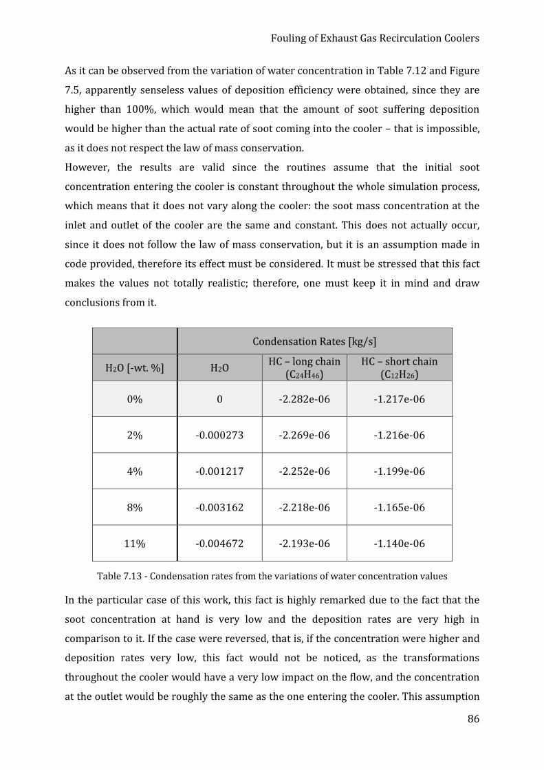
Fouling of Exhaust Gas Recirculation Coolers
86
As it can be observed from the variation of water concentration in Table 7.12 and Figure
7.5, apparently senseless values of deposition efficiency were obtained, since they are
higher than 100%, which would mean that the amount of soot suffering deposition
would be higher than the actual rate of soot coming into the cooler – that is impossible,
as it does not respect the law of mass conservation.
However, the results are valid since the routines assume that the initial soot
concentration entering the cooler is constant throughout the whole simulation process,
which means that it does not vary along the cooler: the soot mass concentration at the
inlet and outlet of the cooler are the same and constant. This does not actually occur,
since it does not follow the law of mass conservation, but it is an assumption made in
code provided, therefore its effect must be considered. It must be stressed that this fact
makes the values not totally realistic; therefore, one must keep it in mind and draw
conclusions from it.
Table 7.13 - Condensation rates from the variations of water concentration values
In the particular case of this work, this fact is highly remarked due to the fact that the
soot concentration at hand is very low and the deposition rates are very high in
comparison to it. If the case were reversed, that is, if the concentration were higher and
deposition rates very low, this fact would not be noticed, as the transformations
throughout the cooler would have a very low impact on the flow, and the concentration
at the outlet would be roughly the same as the one entering the cooler. This assumption
Condensation Rates [kg/s]
H2O [-wt. %] H2O HC – long chain
(C24H46) HC – short chain
(C12H26)
0% 0 -2.282e-06 -1.217e-06
2% -0.000273 -2.269e-06 -1.216e-06
4% -0.001217 -2.252e-06 -1.199e-06
8% -0.003162 -2.218e-06 -1.165e-06
11% -0.004672 -2.193e-06 -1.140e-06

Fouling of Exhaust Gas Recirculation Coolers
87
made by the supplier of the routines is valid as it performs the calculations solely for the
equilibrium state. They fundamentally “remove” the time component and, therefore, the
deposited particles obtained are not to be deposited “in every moment” but rather at an
infinite length of time, where a steady state is reached.
This is particularly evidenced by Table 7.13, which displays the condensation rates
corresponding to this water concentration variation – also after six iterations, just like
the deposition rates of the particles, where it displays a higher value.
From the observation of Table 7.13, one can conclude that the higher the water vapor
concentration, the greater its condensation is, and the smaller are the condensation
rates for the HC. In order to understand why this occurs, the temperature at the
interface between the deposit layer and the flow was determined. The results for the
heat flow that crosses the deposit layer was obtained with Fluent and then the matching
temperature was procured from the Equation (7.2), assuming that the temperature at
the wall is constant and equal to the water temperature. The results obtained are
displayed in Table 7.14.
As the interface temperature increases with the rise in water concentration, one can
understand why condensation of HC decreases: a higher temperature induces less
condensation of this species at the interface. However, despite the influence from the
HC, the water displays a much greater influence, as its condensation rate is of 3
magnitude orders higher. This has a great influence on the value of the deposition
efficiency, as more condensed water will divert many more particles to the surface, that
is, the diffusiophoresis effect is enhanced by a higher concentration gradient caused by
Table 7.14 - Results on the interface temperature between deposit layer and the flow, for variation of water concentration
H2O [-wt. %] Deposit
Thickness [mm]
Thermal Conduct.
[𝑊
(𝑚 𝐾)]
Area [m2] Heat
Transfer [W]
𝑇𝑖𝑛𝑡𝑒𝑟𝑓𝑎𝑐𝑒
[°C]
2% 0.1522 0.1522 0.004874 170.76 31.87
4% 0.2011 0.2011 0.004824 170.21 32.94
8% 0.2061 0.2061 0.004819 170.09 33.22
11% 0.6709 0.6709 0.004352 175.01 69.78
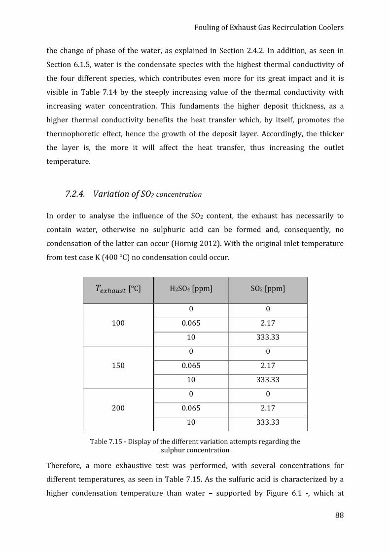
Fouling of Exhaust Gas Recirculation Coolers
88
the change of phase of the water, as explained in Section 2.4.2. In addition, as seen in
Section 6.1.5, water is the condensate species with the highest thermal conductivity of
the four different species, which contributes even more for its great impact and it is
visible in Table 7.14 by the steeply increasing value of the thermal conductivity with
increasing water concentration. This fundaments the higher deposit thickness, as a
higher thermal conductivity benefits the heat transfer which, by itself, promotes the
thermophoretic effect, hence the growth of the deposit layer. Accordingly, the thicker
the layer is, the more it will affect the heat transfer, thus increasing the outlet
temperature.
7.2.4. Variation of SO2 concentration
In order to analyse the influence of the SO2 content, the exhaust has necessarily to
contain water, otherwise no sulphuric acid can be formed and, consequently, no
condensation of the latter can occur (Hörnig 2012). With the original inlet temperature
from test case K (400 °C) no condensation could occur.
Table 7.15 - Display of the different variation attempts regarding the sulphur concentration
Therefore, a more exhaustive test was performed, with several concentrations for
different temperatures, as seen in Table 7.15. As the sulfuric acid is characterized by a
higher condensation temperature than water – supported by Figure 6.1 -, which at
𝑇𝑒𝑥ℎ𝑎𝑢𝑠𝑡 [°C] H2SO4 [ppm] SO2 [ppm]
100
0 0
0.065 2.17
10 333.33
150
0 0
0.065 2.17
10 333.33
200
0 0
0.065 2.17
10 333.33

Fouling of Exhaust Gas Recirculation Coolers
89
approximately 1 bar corresponds to 350 °C, one would understand why no condensation
was observed with such a high inlet temperature (400 °C). Thence, lower inlet
temperatures were used to attempt to observe the effect of sulfuric acid condensation,
as seen in Table 7.15. Nonetheless, all the other initial conditions from point K were
maintained.
𝑇𝑖𝑛𝑙𝑒𝑡 = 100 °𝐶
H2SO4 [ppm]
Deposit Thickness
[mm]
Deposition Efficiency
[%]
𝑇𝑜𝑢𝑡 CHT [°C]
𝑇𝑜𝑢𝑡 Fouling
[°C]
Thermal Conduct.
[𝑊
(𝑚 𝐾)]
0 0.4423 31.370
79.44
80.61 0.5411
0.065 0.4361 110.222 80.63 0.5230
10 0.4358 135.853 80.64 0.5202
Table 7.16 - Results of the variation of sulfuric acid concentration on point K, with an inlet temperature of 100 °C
𝑇𝑖𝑛𝑙𝑒𝑡 = 150 °𝐶
H2SO4
[ppm]
Deposit Thickness
[mm]
Deposition Efficiency
[%]
𝑇𝑜𝑢𝑡 CHT [°C]
𝑇𝑜𝑢𝑡 Fouling
[°C]
Thermal Conduct.
[𝑊
(𝑚 𝐾)]
0 0.3435 31.275
115.77
117.39 0.3917
0.065 0.3338 109.793 117.41 0.5023
10 0.3331 135.437 117.42 0.4999
Table 7.17 - Results of the variation of sulfuric acid concentration on point K, with an inlet temperature of 150 °C

Fouling of Exhaust Gas Recirculation Coolers
90
𝑇𝑖𝑛𝑙𝑒𝑡 = 200 °𝐶
H2SO4 [ppm]
Deposit Thickness
[mm]
Deposition Efficiency
[%]
𝑇𝑜𝑢𝑡 CHT [°C]
𝑇𝑜𝑢𝑡 Fouling
[°C]
Thermal Conduct.
[𝑊
(𝑚 𝐾)]
0 0.2967 31.183
151.42
153.68 0.4823
0.065 0.2849 109.336 153.70 0.4581
10 0.2846 134.909 153.71 0.4600
Table 7.18 - Results of the variation of sulfuric acid concentration on point K, with an inlet temperature of 200 °C
When looking at Tables 7.16, 7.17 and 7.18 one can see that a significant variation in
sulphur content leads to almost no variation of the final deposit thickness at the steady-
state. This can be explained by the fact that the concentration of sulfur, compared to the
concentration of water vapor existing in the exhaust gas is extremely small. However,
the values of the deposition efficiency suffer a much greater discrepancy. In order to
understand what caused this, an analysis of the forces in place was undertaken: the
values of forces and mass flow rates of the several deposition mechanisms were
obtained. The results are displayed in Tables 7.19 and 7.20. Regarding the forces acting
on the cooler, one can observe that, even though the sulphur concentration changes, no
change is visible in the forces. For the cases of 150 °C and 200 °C for the water
temperatures, no significant variation of these values was seen, so they are not shown.
Forces [N] at 𝑇𝑖𝑛𝑙𝑒𝑡 = 100 °𝐶
H2SO4 [ppm]
Drag Lift Thermal Sticking
0 5,00E-14 1,50E-14 1,22E-13 3,90E-13
0.065 5,00E-14 1,50E-14 1,22E-13 3,90E-13
10 5,00E-14 1,50E-14 1,22E-13 3,90E-13
Table 7.19 - Results of the forces acting in the cooler for the different sulphur concentrations at 100 °C of exhaust gas inlet temperature

Fouling of Exhaust Gas Recirculation Coolers
91
Mass Flow Rates [kg/s] at 𝑇𝑖𝑛𝑙𝑒𝑡 = 100 °𝐶
H2SO4 [ppm]
Thermophoresis Diffusiophoresis Impaction Diffusion
0 7,00E-07 5,00E-05 2,00E-10 5,00E-08
0.065 7,00E-07 5,00E-05 2,00E-10 5,00E-08
10 6,00E-07 5,00E-05 2,00E-10 5,00E-08
Table 7.20 - Results of the mass flow rates from the deposition mechanisms in the cooler for the different sulphur concentrations at
100 °C of exhaust gas inlet temperature, for particle size P3
This leads to the conclusion – since no remarkable variation was seen in the parameters
obtained in Tables 7.19 and 7.20 - that the impact of the sulfuric acid in the overall
fouling effect is almost non-existent. It displays no impact whatsoever on the variation of
the forces that cause the sticking of the particles to the wall. This relates to the sticking
factor, which will be further ahead mentioned and discussed.
Condensation Rates [kg/s]
H2SO4 [ppm] H2O HC – long chain
(C24H46) HC – short chain
(C12H26) H2SO4
0 -0.0002913 -2.336E-06 -1.277E-06 0.0
0.065 -0.0002912 -2.336E-06 -1.277E-06 -9.63E-10
10 -0.0002913 -2.336E-06 -1.277E-06 -1.48E-07
Table 7.21 - Condensation rates of the four different species for the variation of sulphur concentration at 100 °C with the presence of water
The condensation rates were also determined and analysed, to allow a perception of the
relationship between the amounts of the different condensate forming species, Table
7.21. As one can conclude by observing the table, with variation of sulfuric acid
concentration, only its condensation rate is altered. The other species remains the same,
as expected. Furthermore, it is clear that the condensation rate of the sulfuric is the one
that displays lower order values. This order difference is especially great when
compared to the water vapor, which shows and proves how small the impact of the

Fouling of Exhaust Gas Recirculation Coolers
92
sulphur in the overall deposition is. Regarding the other two temperature cases of 150
°C and 200 °C the condensation rates of HC and SO2 slightly increase, whereas the one of
water slightly decreases, as the exhaust temperature is increased - but keeping the same
relationship in the orders of magnitude.
In Table 7.22 are depicted the results of the variation of sulphur concentration, but this
time without the presence of water, in order to understand the difference between the
deposition efficiency values. By taking a closer look at it, one can see that the deposition
efficiency increases with rising sulphur concentration. The deposition efficiency
provides a measurement for the velocity of deposition, but it does not necessarily mean
that there will be more deposition and, therefore, a thicker layer in the state of
equilibrium. In both results, with or without the presence of water vapor, one can see
the influence of the sulphur in the deposition efficiency.
Table 7.22 - Results for the variation of sulphur concentration values, with null concentration of water vapor in the exhaust gas
𝑇𝑒𝑥ℎ𝑎𝑢𝑠𝑡 [°C]
H2SO4 [ppm]
Deposit Thickness
[mm]
Deposition Efficiency
[%]
𝑇𝑜𝑢𝑡 CHT [°C]
𝑇𝑜𝑢𝑡 Fouling
[°C]
Thermal Conductivity
[𝑊
(𝑚 𝐾)]
100
0 0.3928 0.633
79.44
81.21 0.3077
0.065 0.3867 3.153 81.28 0.2903
10 0.3857 3.216 81.28 0.2888
150
0 0.3184 0.991
115.77
118.28 0.3034
0.065 0.3092 4.928 118.43 0.2768
10 0.3086 4.972 118.43 0.2761
200
0 0.2946 1.358
151.42
154.97 0.2994
0.065 0.2827 6.754 155.25 0.2643
10 0.2825 6.792 155.25 0.2641

Fouling of Exhaust Gas Recirculation Coolers
93
However, this influence is magnified in the results from Tables 7.16 to 7.18 due to the
condensation of water. An influence in the deposit thickness is then visible when the
thermal conductivity obviously varies, which is also clear in both cases. A drop in the
thermal conductivity explains a slimmer deposition rate, because it impedes the heat
transfer, which will reduce the thermophoretic effect and, therefore, the soot deposition.
As one knows beforehand that the sulphur is expected to have no influence in the
deposition layer when the concentration of water is null, this is corroborated by the
information in Table 7.22. The variation of deposit thickness is very small for every used
exhaust gas temperature; therefore, the sulfuric acid plays almost no role in the
deposition. And when it is in the presence of water vapor its amount is so small
compared to the water, that its influence is almost non-existent. Furthermore, it is also
important to take notice of the sticking factor associated with the condensation of the
sulfuric acid, which explains why there is practically no influence of this species with the
variation of its concentration. This parameter is further explained in Section 7.3.
7.2.5. Variation of the exhaust mass flow
In order to assess the variation of the exhaust mass flow input, the other values chosen
for this study were values also used by Völk and Hörnig (2011) in other measurements,
which are not depicted in this thesis. The other boundary conditions are the original
values from test case K, apart from the �̇�𝑒𝑥ℎ𝑎𝑢𝑠𝑡.
Table 7.23 - Results on the single variation of exhaust mass flow for point K
�̇�𝑒𝑥ℎ𝑎𝑢𝑠𝑡 [kg/h]
Deposit Thickness
[mm]
Deposition Efficiency
[%]
𝑇𝑜𝑢𝑡 CHT [°C]
𝑇𝑜𝑢𝑡 Fouling [°C]
Thermal Conductivity
[𝑊
(𝑚 𝐾)]
Heat transfer
[kW]
2 0.7057 2.144 277.05 285.26 0.2931 262.87
4 0.3375 2.829 286.98 294.50 0.2871 483.27
5.5 0.1471 3.500 290.73 295.08 0.2830 642.45
7 0.0143 1.053 295.66 295.73 0.2064 780.78
9 0.0 0.000 298.19 298.19 - 979.51

Fouling of Exhaust Gas Recirculation Coolers
94
As it can be observed in Table 7.23 and Figure 7.6, the higher the exhaust mass flow, the
less deposit thickness is built, because a higher mass flow implies a higher flow velocity,
which impedes the heat transfer since the particles have less time to flow across the
cooler. Also, a greater velocity may cause higher removal forces, which in the case for 9
kg/h, they remove the entire deposit layer. As mentioned in Section 2.7.2, there is a
critical velocity for every particle size above which the particle is removed from the wall.
Looking at Figure 2.14 from the same section, one can see that in the particle range
existing in the EGR coolers the critical flow velocities range from 40 to 280 m/s. In fact,
the corresponding velocity for a 9 kg/h flow in the used geometry is around 60.4 m/s,
which already falls within this interval, explaining why the removal of the deposit layer
occurs. The lower the exhaust mass flow, the lower the velocity of the fluid, as long as
there is no variation of the density of the flow. The lower the velocity, the more heat
transfer occurs, thus favoring the deposition of soot by thermophoresis.
However, regarding the deposition efficiency, one would expect it to decrease with
decreasing deposit thickness, as the deposition is promoted from the beginning of the
deposition process, i.e. in the initial iterations. As explained in Section 2.5 when a
turbulent state is present, it helps to mix the particles, which promotes the formation of
the deposit layer, thus increasing the deposition efficiency. Nonetheless, when the
velocity in this turbulent state is too high, it will stop promoting soot deposition and will
begin to act as a removal mechanism, since the velocity has crossed the value for of
Figure 7.6 - Evolution of the deposit thickness and deposition efficiency with the variation of exhaust mass flow for test case K

Fouling of Exhaust Gas Recirculation Coolers
95
critical velocity defined in Section 2.7.2 – this is what happens between the cases for 5.5
kg/h and 9 kg/h in Table 7.23. As it can be seen, the deposition efficiency at 7 kg/h is
already decreasing and by 9 kg/h it has reached zero.
Concerning the temperature distribution, when looking at the 𝑇𝑜𝑢𝑡 of the CHT analysis,
one could question why the temperature at the outlet is approximately 21 °C higher for
the higher velocity case, comparing to the lower velocity case, even though the inlet
temperature is equal for all of the cases, 400 °C. The answer lies in determining the
amount of energy transferred in the CHT process. Through the thermal energy balance
𝑄 = �̇� ∙ 𝑐𝑝 ∙ ∆𝑇, one can easily determine the energy transfer in every process, assuming
the specific heat capacity of air at 400 °C. Even though the temperature is higher for the
9 kg/h case, the energy transfer is almost four times higher than in the 2 kg/h case. The
increase in velocity diminishes the overall heat transfer, thus increasing the outlet
temperature.
It can also be noted that the thermal conductivity decreases with increasing exhaust
mass flow. As previously mentioned, the amount of soot and condensates are the main
determining factors for the thermal conductivity of the final deposit layer. In this case, as
the exhaust mass flow is increased, the amount of condensate species flowing in
increases relatively to the soot amount, as the soot mass flow remains constant.
Therefore, in theory, the thermal conductivity should increase due to a bigger amount of
condensates present. However, due to the higher flow velocity, the temperatures in the
deposit layer decrease, thus decreasing the level of condensation - even though the
species concentration is higher.
�̇�𝑒𝑥ℎ𝑎𝑢𝑠𝑡[kg/h] Condensation Rates [kg/s]
HC – long chain (C24H46) HC – short chain (C12H26)
2 -2.525E-06 -1.365E-06
4 -2.333E-06 -1.238E-06
5.5 -2.282E-06 -1.217E-06
7 -2.277E-06 -1.233E-06
Table 7.24 - Condensation rates of the HC present in the flow, for exhaust mass flow variation of test case K

Fouling of Exhaust Gas Recirculation Coolers
96
This is verified in Table 7.24, where one can clearly see that the HC condensation rates
decrease – the only condensate forming species present in this section - as the flow
increases, hence explaining the decreasing value of thermal conductivity.
Fundamentally, a higher exhaust mass flow prevents the creation of a deposit layer,
which leads to the non-occurrence of the deterioration of the cooler’s performance, but
will also lead to higher outlet temperatures. When comparing the values for 2 kg/h and
9 kg/h one can see that the first has the highest deposit thickness but also the lowest
temperature at the outlet (in CHT and fouling analysis, after the deterioration of the
performance), while the latter has no deposit thickness and, however, has the highest
outlet temperature.
7.2.6. Variation of the soot mass flow
�̇�𝑠𝑜𝑜𝑡 [mg/h]
Deposit Thickness
[mm]
Deposition Efficiency [%]
𝑇𝑜𝑢𝑡 CHT [°C] 𝑇𝑜𝑢𝑡
Fouling [°C]
Thermal Conductivity
[𝑊
(𝑚 𝐾)]
20 0.1512 1.560
290.73
294.99 0.2976
45 0.1471 3.500 295.08 0.2830
90 0.1415 6.960 295.22 0.2619
150 0.1358 11.530 295.40 0.2407
Table 7.25 - Results on the single variation of soot mass flow for point K
The effect observed in the Table 7.25 and Figure 7.7 is that, with increasing soot mass
flow, the deposition efficiency is clearly increased, whereas the deposit thickness slightly
decreases. A higher soot mass flow means that, for the same amount of condensates,
there is a bigger amount of soot. This will decrease the thermal conductivity because, as
stated before in Section 6.1.6., the soot is characterized by a thermal conductivity of 0.1
W/(m K) whereas all the condensates possess higher values.
Therefore, with increasing soot mass flow, a thinner deposit layer will have the same
isolative effect as a thicker one with less overall soot, as both the final density of the
deposit layer and its thermal conductivity will be different.

Fouling of Exhaust Gas Recirculation Coolers
97
Figure 7.7 - Evolution of the deposit thickness and deposition efficiency with the variation of soot mass flow for test case K
The values obtained in this section are very satisfactory, as the thicker the deposit layer
is, the higher will be the thermal conductivity, which matches the theoretical expected
tendency. The more soot is present in the flow (compared to the existing condensates),
the thinner will the deposit layer be at the final steady-state in the cooler.
When analysing the temperature, it is visible that there is almost no variation. This may
lie on the fact that the flow boundary conditions are the same and the paired variation of
the deposit thickness and thermal conductivity changes in a way that provides the same
final temperature.
Finally, regarding the deposition efficiency, it is understandable that, with a higher
amount of soot particles, with all the other boundary conditions remaining unchanged,
the deposition efficiency will increase. Since there is a higher concentration of soot
particles flowing at every given point through the cooler, more particles will be easily
driven to the wall, as the deposition rate of each one of the particle classes will be
incremented.
7.3. Sticking Factor
One crucial factor for the deposition of soot is the sticking factor. It is an empirical value
used in the calculations of the routines which accounts for the impact of HC and H2SO4

Fouling of Exhaust Gas Recirculation Coolers
98
(but not H2O) condensation on the probability of soot to be deposited at the wall; it is yet
only relevant when soot deposition occurs. After being obtained, this parameter is then
multiplied by the sum of the deposition mass flow rates, thus influencing the overall
deposit building.
In order to understand the different impact caused by these two condensate forming
species, the sticking factor of each one of them was determined – after six iterations, for
an analogy with the deposition rates -: simulations were carried out with different
concentrations of SO2 and zero concentration of HC, and vice-versa. The results are
displayed in Tables 7.26 and 7.27:
SO2 [ppm] Sticking factor [-]
0 1
0.05 1 – 3.22
0.1 1.59 – 4.11
0.5 3.80 - 5
2.17 5
333.33 5
Table 7.26 - Determined values for the sticking factor concerning solely SO2
concentration, after six iterations, for test case K
Since the sticking factor depends on local soot deposition rate, it is not constant
throughout the entire cooler; therefore, in Table 7.26 the range of sticking factors
obtained for the SO2 concentration is shown. One can conclude that the variation of
sulphur does not play almost any influence in the results, as the only different noticed is
between 0 and 2.17 ppm, which are extremely low quantities, especially when compared
with the amount of water present, as seen before in section 7.3.5. As the value 5 is the
maximum possible for the sticking factor of this species, one can understand why from
2.17 ppm onwards there is no variation of its influence: the maximum sticking effect it
can provide to the deposit layer has already been reached. The maximum value of 5 has
empirically been derived by the supplier of the UDFs.

Fouling of Exhaust Gas Recirculation Coolers
99
When comparing the values from Tables 7.10 and 7.27 it is possible to conclude that the
sticking factor has an influence in the deposition due to the present of HC. From around
300 ppm the value of the deposit thickness begins to change very scarcely and from
around 700 ppm it has totally stagnated. Analogously, the same tendency is observed in
Table 7.27 for the result of the sticking factor due to the presence of HC. Since the
maximum value for the sticking factor from HC has been defined in the routines as 2.3,
one can see that the values obtained have stagnated because it has reached its
maximum. This is especially clear in Figure 7.8.
HC [ppm] Sticking factor [-]
0 1.000
200 2.270
300 2.289
350 2.290
430 2.298
450 2.293
750 2.296
1000 2.297
2000 2.298
Table 7.27 - Determined values for the sticking factor concerning solely HC concentration, after six iterations, for test case K
Figure 7.8 - Evolution of the sticking factor with the variation of HC concentration, for test case K, after 6 iterations

Fouling of Exhaust Gas Recirculation Coolers
100
According to Table 6.2 it is clear why, even though the HC has got a lower sticking factor
than the SO2, the impact of the first one in the deposit building is much greater as it
possesses a much higher molecular weight, thus having a greater influence in the
outcome of the fouling effect than the sulphur. Also, its thermal conductivity is slightly
higher, as seen in Table 6.3, which may promote the growth of the deposit thickness, as
it facilitates the heat transfer, thus increasing the effect of thermophoresis.
7.4. Simulations – Motor Test Bench
In this section, the two different test cases described in Section 5.6 are going to be
pursued. The results of the measurements from Völk and Hörnig (2011) for the variation
of 𝑇𝑤𝑎𝑡𝑒𝑟, Figures 7.9 and 7.10, depict the evolution of the deposit thickness along the
cooler for these two test cases.
Dep
osi
t T
hic
kn
ess
[mm
]
Figure 7.10 - Results of Deposit Thickness for Test Case 2 (adapted to English)
Figure 7.9 - Results of Deposit Thickness for Test Case 1 (adapted to English)
Dep
osi
t T
hic
kn
ess
[mm
]

Fouling of Exhaust Gas Recirculation Coolers
101
According to Völk and Hörnig (2011), in Test Case 1 of motor test bench, regarding the
curves for 20°C and 40 °C it is not possible to obtain a full picture of the soot deposition
by condensation throughout the entire cooler because of the deposit gaps seen in Figure
7.9. However, it allows to conclude that, in the final part of the cooler an effect of wash-
out is observed, due to the condensation of water. This strong water condensation and
the consequent areas of deposit removal in the cooler lead to an unsteady growth of the
deposit layer, as it can be seen in Figure 7.9. In Figure 7.11 the measured mass
deposition for each of the used water temperatures in Test Case 1 is displayed and the
results for 40 °C, 60 °C and 80 °C follow the trend that, with lower water temperatures,
higher condensation rates are observed which lead to an increased deposition growth.
The only case that does not verify this condition is the one of 20 °C, due to the fact that
the water condensation is so strong that it continuously resists the building of the
deposit layer (Völk, 2014). The case for 40 °C also experiences wash-out, reason why
there are gaps in the deposit layer and it is lower than for 60 °C and 80 °C in some cases;
however, as the condensate mass flow is lower than at 20 °C, it is not enough to
significantly decrease the overall deposited mass, as it can be concluded by Figure 7.11.
The obtaining of an equilibrium state of the fouling process sets up at thinner deposit
layers with increasing water temperature. This happens due to the smaller amount of
condensates in the layer, which makes it drier and with a lower adhesive behavior.
Analysing the results from Test Case 1 and Test Case 2 in their work, it is to conclude
that the tendency for greater deposit thickness with decreasing cooling temperature is
confirmed with the increase in exhaust mass flow rate.
Dep
osi
ted
mas
s [g
]
Figure 7.11 - Deposited mass for the four water temperature cases of Test Case 1 in motor test bench from Völk and Hörnig (2011)

Fouling of Exhaust Gas Recirculation Coolers
102
Regarding the Test Case 2 results presented in Figure 7.10, the increased mass flow rate
and the higher inlet temperature of 380 °C both contribute to the avoidance of
condensation water films forming at the wall. Therefore, it is clearly observed that, even
at water temperature of 20 °C, the wash-out effect does not take place; thus, increasing
the deposit thickness at lower temperature, verifying the above described tendency.
Furthermore, with the increase in moisture content in the layer – as it does not
condense to cause wash-out -, the adhesive force is strong enough to promote the
increase of the deposit layer, despite a greater gas shear stress caused by the higher flow
rate (Völk, 2014). The results for the simulations performed on Test Case 1 are
displayed in Tables 7.28 and 7.29, as follows:
Table 7.28 - Results for Test Case 1 from motor test bench, with 350 ppm of HC and 2% of H2O, and the respective results from Völk and Hörnig (2011)
Simulation Results Measurement
Results
𝑇𝑤𝑎𝑡𝑒𝑟
[°C]
Deposit Thick. [mm]
Dep. Eff. [%]
𝑇𝑜𝑢𝑡 CHT [°C]
𝑇𝑜𝑢𝑡 Fouling
[°C]
Thermal Conduct.
[𝑊
(𝑚 𝐾)]
Deposit
Mass [g]
Deposit
Thick.
[mm]
Dep.
Mass
[g]
20 0.00861 3.799 226.79 226.84 0.1790 7.56E-04 0 – 0.30 0.5805
40 0.00328 0.369 233.14 233.16 0.1175 2.88E-04 0 – 0.55 1.2125
60 0.00205 0.268 239.88 239.83 0.1226 1.80E-04 0.45 0.9656
80 0.00183 0.300 244.84 244.84 0.2114 1.61E-04 0.40 0.8495
Dep
osi
t T
hic
kn
ess
[mm
]
Figure 7.12 - Plot of the simulated evolution of deposit thickness throughout the entire cooler length for Test Case 1 at 20 °C of water temperature, with 350 ppm
of HC and 2% of H2O

Fouling of Exhaust Gas Recirculation Coolers
103
For the simulation of test case 1, according to Table 5.6, there is an interval of the values
for the input in HC and H2O concentration. Therefore, for the simulations performed,
two pairs of extreme values were adopted, and Table 7.28 displays the values for 350
ppm of HC and 2% of water, while Table 7.29 displays the values for 450 ppm of HC and
11% of water. In this section of the work accomplished by Völk and Hörnig (2011),
regarding the measurements of the motor test bench, no information is mentioned on
the contents of the water concentration. Therefore, as seen in Section 2.2.1, the interval
of the possible water extreme concentrations is between 2% and 11%; the simulations
performed in this dissertation took those values as the possible best and worst-case
scenario, when it comes to water content damaging the performance of the cooler.
Figure 7.12 displays a plot of the evolution of deposit thickness throughout the cooler
for the case of 20 °C from Table 7.28. It shows that the simulated evolution of the deposit
thickness is not constant throughout the cooler which, despite not showing the same
shape as the result from their measurements, is a plausible result. The greatest deposit
thickness is depicted at the entrance of the cooler - the area where the thermophoretic
force is at its highest -, because the temperature difference exhibits its maximum value.
From the geometry defined in Section 5.1, one knows that the entrance of the tube is 65
mm after the entrance in the cone. Knowing that the mesh defined in Fluent for the
simulations has the zero (beginning of the cone) at 28 mm in the z-axis, it is clear that
the tube starts at 93 mm, where the first point is depicted in Figure 7.12; and the end of
the tube is at 253 mm. From about 120 mm no deposit thickness is visible, which is due
to the high mass flow rate (which causes high shear stress) associated with a weakened
effect of thermophoresis, as the temperature difference is not as great as at the entrance.
Therefore, the removal forces surpass the deposition mechanisms. This occurs in both
Figure 7.12 and 7.13. However, this effect is much weaker in the experiment.

Fouling of Exhaust Gas Recirculation Coolers
104
Table 7.29 - Results for Test Case 1 from motor test bench, with 450 ppm of HC and 11% of H2O
In Table 7.29 and Figure 7.13 the results for the highest extreme pair of HC and H2O
values is shown, and they both display the same tendencies as the case before, however
with rather higher values, since the increased concentrations of HC and H2O promote the
condensation of these species, increasing the impact of the soot deposition.
The difference between Figures 7.12 and 7.13 is not great, but it can still be drawn.
Despite the fact that the first case reaches a higher thickness value, the second curve is
wider and the deposit layer is more spread through the length of the cooler than the first
one. For this reason, the second case – matching the higher HC and H2O concentration
values – displays an overall higher deposit thickness.
Simulation Results Measurement
Results
𝑇𝑤𝑎𝑡𝑒𝑟
[°C]
Dep. Thick. [mm]
Dep. Eff. [%]
𝑇𝑜𝑢𝑡 CHT [°C]
𝑇𝑜𝑢𝑡 Fouling
[°C]
Thermal Conduct.
[𝑊
(𝑚 𝐾)]
Deposit
Mass [g]
Deposit
Thick.
[mm]
Dep.
Mass
[g]
20 0.0169 31.151 226.79 226.90 0.3244 1.48E-03 0 – 0.30 0.5805
40 0.0144 20.271 233.14 233.21 0.2254 1.26E-03 0 – 0.55 1.2125
60 0.0023 0.4700 239.88 239.83 0.1159 2.02E-03 0.45 0.9656
80 0.0019 0.290 244.84 244.84 0.1251 1.67E-03 0.40 0.8495
Dep
osi
t T
hic
kn
ess
[mm
]
Figure 7.13 - Plot of the evolution of deposit thickness throughout the entire cooler length for test case 1 at 20 °C of water temperature, with 450 ppm of HC and 11% of H2O

Fouling of Exhaust Gas Recirculation Coolers
105
In addition, one can see that in both cases the maximum deposit thickness is,
respectively, 0.08 and 0.07 mm. Nonetheless, as the overall deposit thickness is
determined as an Area-Weighted Average, the value is averaged through the entire tube
area, and as in most of it there is no deposit, then one can easily understand why the
overall values are smaller and, respectively: 0.00861 and 0.0169 mm.
When analysing the deposit thickness evolution with the water temperature (in both
cases), a single tendency is perceived. With increasing water temperature, the deposit
thickness increases due to the higher amount of condensates. However, contrarily to the
results obtained by Völk and Hörnig (2011), in the case for 20 °C, no wash-out effect is
observed, because the routines do not contemplate this effect: a decrease of soot
deposition due to condensation is not possible. Therefore, the deposit thickness does not
decrease as it theoretically should.
In order for the deposited mass to be obtained, the approximate value of the deposit
layer is determined – as the deposit thickness is an approximate value, it is not possible
to acquire the exact value – and then multiplied by the density of the deposit layer. As
previously mentioned, in the routines a constant value for this density is assumed and it
is 17.5 kg/m3. As the deposit layers are extremely small for both results in Tables 7.28
and 7.29, it is understandable why the mass values are so small.
Regarding the results for the Test Case 2, the same approach was used. However, the
results obtained for the extreme highest concentration pair were of zero deposit
thickness and deposition efficiency, i.e. there is no occurrence of soot deposition. This
extreme point is the one corresponding to 20 °C on the water side, with 450 ppm of HC
and 11% of H2O, where the deposition would be reinforced by a greater thermophoretic
effect – grounded on a greater temperature difference - and higher condensation rates to
promote diffusiophoresis - due to greater condensate forming species concentration.
Therefore, since this is the point which would display stronger deposition efficiency, as
it occurs in Test Case 1, and nothing occurs, then it is safe to conclude that for the other
simulation points there is also no appearance of a soot deposit.
From the physical point of view, it is easy to comprehend why there is no formation of a
deposit layer in the simulation of Test Case 2. With a tube geometry as small as the one
used in this study and an exhaust mass flow of 15 kg/h the corresponding flowing

Fouling of Exhaust Gas Recirculation Coolers
106
velocity is of approximately 369 km/h, i.e. about 102 m/s. Keeping in mind what is
explained in Section 2.7.2, when the flow velocity increases and crosses the boundary of
critical velocity, removal by gas shear stress starts to occur. The interval of critical
velocities is dependent on the particle size and ranges from 40 m/s to 280 m/s. In this
particular case, the velocity of 102 m/s falls in the middle of that range, which, allied to
the fact that the particle distribution for this test bench displays a greater amount of
particles with bigger size, allows to explain why there is no soot deposition occurring at
all.
The visible difference between the deposit thickness results from the motor and model
test bench are easily explained by the great difference in exhaust mass flow. As seen in
Section 7.2.6, where this parameter was changed, one can see that by 9 kg/h – the mass
flow existing in the motor test bench - in the model test bench, no emerging of a deposit
layer was observed. However, despite the high value of exhaust mass flow in the present
Test Case 1, due to a higher value of soot mass flow it is still possible to observe the
appearance of the deposit layer, albeit being quite thin. Nonetheless, with a higher soot
mass flow, it is no longer possible to observe the emerging of the deposit layer in Test
Case 2, since the exhaust mass flow displays a value of 15 kg/h. The fact that it does
emerge in the experiments conducted by Völk and Hörnig (2011) might either be caused
by errors in their measurements or invalid model parameters.
Furthermore, the work accomplished by Völk (2014) shows a result for the lowest
exhaust mass flow, even though the result is time-dependent.
Dep
osi
t T
hic
kn
ess
[mm
]
Figure 7.14 - Evolution of the deposit thickness for 4.5 kg/h mass flow, with exhaust temperature of 300 °C and water
temperature of 80 °C

Fouling of Exhaust Gas Recirculation Coolers
107
However, as it will be later mentioned in Section 7.4.2, when the measurements are
endured for about 20 hours one can already consider the result to be in a state of
equilibrium. Concretely in the case exhibited in Figure 7.14, the experiment was pursued
for 8 hours and, carefully analysing the depicted curve, one can observe that from the
value of 0.3 mm the deposit thickness growth is slowly starting to decrease. The results
obtained for the simulations with the same boundary conditions are presented in Table
7.30. When comparing these results with the value from the curves in Figure 7.14, a
resemblance is seen. That is, for an exhaust mass flow as low as 4.5 kg/h, the results
obtained from the simulations with the user defined functions are very similar to the
ones form the experiment measures: the values obtained were around 0.3 mm and
through Figure 7.14 one can see that, even though the value has not yet stagnated, it is
starting to decrease the curvature, thus placing the constant value not much further.
This leads to the conclusion that the routines provided are valid and deliver fairly good
results at low exhaust mass flow conditions.
Deposit
Thickness
[mm]
Deposition
Efficiency
[%]
𝑇𝑜𝑢𝑡 CHT [°C]
𝑇𝑜𝑢𝑡 Fouling
[°C]
Thermal Conduct.
[𝑊
(𝑚 𝐾)]
450 ppm HC;
11% H2O 0.3143 7.349 239.42 244.43 0.2137
350 ppm HC;
2% H2O 0.3097 6.578 239.42 244.48 0.2072
Table 7.30 - Simulation results for 4.5 kg/h mass flow, with exhaust temperature of 300 °C and water temperature of 80 °C
After arriving to this conclusion, one may question why, with a low exhaust mass flow,
the results obtained by the simulations are similar to the values observed by Völk and
Hörnig (2011), whereas with higher values for the exhaust mass flow, extremely lower
values are obtained for the deposit that is built on the wall. In fact, the C-routines work
with several empirical parameters that have an influence in the final results, and were
not addressed in this scope of this work. A conclusion drawn from the analysis above
and from the values obtained both for model and motor test bench is that, as with
increasing exhaust mass flow the deposit built is always smaller, the removal
mechanisms calculated in the routines are far stronger and have a greater impact in the
final results. This is grounded in the fact that there are four empirical factors for the
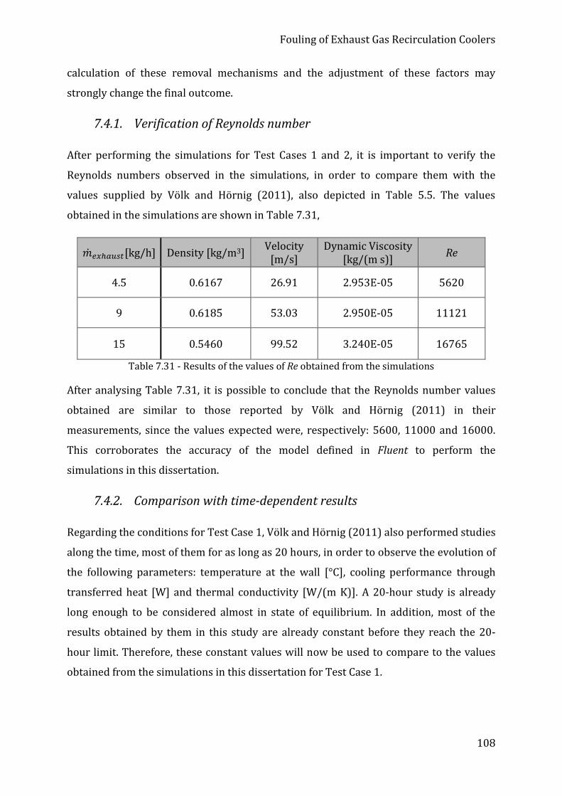
Fouling of Exhaust Gas Recirculation Coolers
108
calculation of these removal mechanisms and the adjustment of these factors may
strongly change the final outcome.
7.4.1. Verification of Reynolds number
After performing the simulations for Test Cases 1 and 2, it is important to verify the
Reynolds numbers observed in the simulations, in order to compare them with the
values supplied by Völk and Hörnig (2011), also depicted in Table 5.5. The values
obtained in the simulations are shown in Table 7.31,
�̇�𝑒𝑥ℎ𝑎𝑢𝑠𝑡[kg/h] Density [kg/m3] Velocity
[m/s] Dynamic Viscosity
[kg/(m s)] Re
4.5 0.6167 26.91 2.953E-05 5620
9 0.6185 53.03 2.950E-05 11121
15 0.5460 99.52 3.240E-05 16765
Table 7.31 - Results of the values of Re obtained from the simulations
After analysing Table 7.31, it is possible to conclude that the Reynolds number values
obtained are similar to those reported by Völk and Hörnig (2011) in their
measurements, since the values expected were, respectively: 5600, 11000 and 16000.
This corroborates the accuracy of the model defined in Fluent to perform the
simulations in this dissertation.
7.4.2. Comparison with time-dependent results
Regarding the conditions for Test Case 1, Völk and Hörnig (2011) also performed studies
along the time, most of them for as long as 20 hours, in order to observe the evolution of
the following parameters: temperature at the wall [°C], cooling performance through
transferred heat [W] and thermal conductivity [W/(m K)]. A 20-hour study is already
long enough to be considered almost in state of equilibrium. In addition, most of the
results obtained by them in this study are already constant before they reach the 20-
hour limit. Therefore, these constant values will now be used to compare to the values
obtained from the simulations in this dissertation for Test Case 1.

Fouling of Exhaust Gas Recirculation Coolers
109
Table 7.32 – Comparison of the simulated values and the measurement values from a 20-hour study for the temperature at the wall and the transferred heat for Test Case 1
Regarding the 60 °C and 80 °C cases in Table 7.32, no more occurrence of wash-out
effects due to condensation can be observed, which makes the evolution of both
parameters more constant and even throughout the time and the length of the cooler, as
seen in Figure 7.9. The process of deposit growth falls with increasing water
temperature and begins to show some parallelism to the wall of the cooler, due to the
decrease of the adhesive behavior of the condensates in the deposit. The fewer amounts
of condensates there is in the deposit, the more constant is the growth of the deposit.
Also, the difference between the result at 40 °C and 60°C regarding the transferred heat
is that the first reaches the level of 150 W only after 20 hours, while the latter is already
in constant heat transfer from about 12 hours. The 40 °C case possesses a water film
overlaid onto the deposit layer, which alters the overall heat transfer. The evolution of
the interface temperature at 80 °C case behaves like that of a clean cooler, due to the low
amount of condensates, which results in an extremely dry soot; the temperature at the
wall matches a state of an homogenous deposit layer (Völk and Hörnig, 2011).
However, the values obtained by simulation are far from matching the temperatures
shown in their measurements. But one cannot forget the disparity of the deposit
thickness values seen above. Taking into consideration the low values obtained in the
Simulation Results
450 ppm HC; 11% H2O
Simulation Results
350 ppm HC; 2% H2O
Measurement Results
Völk and Hörnig (2011)
𝑇𝑤𝑎𝑡𝑒𝑟
[°C]
𝑇𝑤𝑎𝑙𝑙
[°C]
Transferred
heat [W]
𝑇𝑤𝑎𝑙𝑙
[°C]
Transferred
heat [W]
𝑇𝑤𝑎𝑙𝑙
[°C]
Transferred
heat [W]
20 20.94 187.87 21.0 187.28 38 230
40 41.20 170.87 40.71 171.62 58 150
60 60.20 153.72 60.52 153.52 72 150
80 80.42 140.39 80.42 140.91 93 180

Fouling of Exhaust Gas Recirculation Coolers
110
simulations, the results displayed in Table 7.32 are correct and show the expected
tendency, with the evolution in water temperature.
Thermal conductivity
The variation of thermal conductivity in the motor test bench will be analysed in 2
different perspectives: regarding a water temperature variation and an exhaust mass
flow variation. As previously studied, the thermal conductivity increases with increasing
amount of condensates in the deposit layer. Also, the minimal value it can exhibit is 0.1
W/(m K), corresponding to dry soot. The studies from Völk (2014) that provide these
results had the duration of 8 hours.
Table 7.33 - Comparison of the simulated values and the measurement values from an 8-hour study for the thermal conductivity for Test Case 1, with variation of water
temperature between 60 °C and 80 °C
In order to avoid the creation of a condensate film that would increase the
inhomogeneity of the deposit layer, Völk (2014) pursued the measurements only for 60
°C and 80 °C, in order to prevent the overstepping of the dew point.
The value of thermal conductivity for 80 °C is almost constant throughout the entire
time evolution because it is the operating point with the lowest temperature difference;
in addition, its condensation rates of hydrocarbons are fare lower than the others and,
due to the smaller temperature gradient, the deposit thickness almost does not change
along the cooler (Völk and Hörnig, 2011). Therefore, the thermal conductivity is
essentially constant. The decrease in water temperature provides an increase of the
thermal conductivity, due to a lower temperature at the interface of the deposit layer
caused by a better convection transfer coefficient, increasing the deposition of
hydrocarbons. However, the values obtained in the simulations do not match this
Simulation Results
450 ppm HC; 11%
H2O
Simulation Results
350 ppm HC; 2%
H2O
Measurement Results
Völk and Hörnig
(2011)
𝑇𝑤𝑎𝑡𝑒𝑟
[°C] Thermal Conductivity [
𝑊
(𝑚 𝐾)]
Thermal Conductivity
[𝑊
(𝑚 𝐾)]
60 0.1159 0.1226 0.2900
80 0.1251 0.2114 0.2200

Fouling of Exhaust Gas Recirculation Coolers
111
tendency. The magnitude of the values is correct and similar to the ones reported by
Völk (2014), but the evolution observed is not correct, as they decrease with decreasing
water temperature. Nonetheless, this fact may be related to the concentrations
introduced for the simulations, as the values are not exactly known, reason why an
interval of possible values was sought. When carefully analysing the results for the case
with 450 ppm of HC and 11% of H2O in Table 7.33, one can conclude that the difference
between the values is minimal and, therefore, may be considered correct, as the
difference between the corresponding deposit thicknesses is also very small.
On the other hand, as it can be seen on Figure 7.15, the increase of exhaust mass flow
also promotes the increase in thermal conductivity, since the condensate forming
species concentrations flowing in are higher, thus increasing the amount of these
components that can condensate at a certain instant. Furthermore, with the high
thermal conductivity inherent to these components, the overall thermal conductivity of
the layer will increase. In addition, with higher mass flows it is observed that the growth
of thermal conductivity is faster, while by lower mass flow values it tends to stabilize
faster, as it can be noticed in Figure 7.15.
In this ambit, the values obtained for this mass flow variation in the simulations are
presented in Table 7.34. As one could see at the beginning of Chapter 7, the results for an
exhaust mass flow of 15 kg/h were of no deposit formation; therefore, the thermal
Time [h]
Th
erm
al c
on
du
ctiv
ity
[W
/(m
K)]
Texhaust = 300 °C
Twater = 80 °C
Figure 7.15 - Evolution of the thermal conductivity with the exhaust mass flow throughout the time in the measurements of Völk (2014)

Fouling of Exhaust Gas Recirculation Coolers
112
conductivity of this one cannot be assessed. Regarding the cases of 4.5 and 9 kg/h, it can
be observed that in both cases of species concentrations the tendency is the opposite of
what was expected. However, this difference is emphasized in the case for higher
species concentrations.
450 ppm HC;
11% H2O 350 ppm HC;
2% H2O
�̇�𝑒𝑥ℎ𝑎𝑢𝑠𝑡[kg/h] Thermal conductivity [W/(m K)]
4.5 0.2137 0.2072
9 0.1251 0.2114
15 - -
Table 7.34 - Results obtained from the simulations for the values of thermal conductivity on the variation of exhaust mass flow, for 80 °C on
Test Case 1 Notwithstanding, it is sensible to make a deeper analysis of the values. In order to
perform the simulations, the exhaust mass flow has to be directly inserted in Fluent
while in the routines the ratio between soot mass flow and exhaust mass flow is used as
input. In fact, as seen in Table 5.5, the soot mass flow for 9 kg/h is higher than for 4.5
kg/h, respectively the values: 210.01 mg/h and 91.15 mg/h. Accordingly, the ratio
between soot and exhaust mass flow is higher in the 9 kg/h than in the 4.5 kg/h case.
This analysis is made clearer in Table 7.35.
�̇�𝑒𝑥ℎ𝑎𝑢𝑠𝑡[kg/h] �̇�𝑠𝑜𝑜𝑡[mg/h] �̇�𝑠𝑜𝑜𝑡/�̇�𝑒𝑥ℎ𝑎𝑢𝑠𝑡
4.5 91.15 0.02026
9 210.01 0.02233
Table 7.35 - Analysis of the ratios between soot and exhaust mass flow
Finally, it can be concluded that, even though the tendency of thermal conductivity
increase with increase in exhaust mass flow is wrong, the level of the values is correct
and makes sense. In fact, the case of 9 kg/h ought to have higher value of deposit layer
conductivity, as it possesses a higher amount of condensates flowing in. However, the
amount of soot flow in comparison to the whole exhaust flowing in is higher in this case
than at 4.5 kg/h. As soot is the component with lower inherent thermal conductivity, it is
clear why the 9 kg/h case is characterized by lower overall thermal conductivity.

Fouling of Exhaust Gas Recirculation Coolers
113
8. Conclusions and Future Work
8.1. Conclusions
In this dissertation, the topic of study was the numerical simulation of the fouling
phenomenon occurring in the EGR coolers applied to diesel engines. The final goal was
to validate a set of User Defined Functions that, when paired with Fluent, allow for the
correct assessment of the fouling effect. This could be achieved by means of a detailed
study of the boundary conditions that these cooling components are subjected to and
the parameters that have an influence on its performance.
The routines provided have a great potential to describe the physical effects that take
place in the EGR coolers. In the studies that supplied the measurements used as basis of
comparison to the simulations performed, the following effects were reported as playing
a big role in the fouling effect: thermophoresis, condensation, diffusiophoresis,
impaction and diffusion. Through the simulations accomplished in the present
dissertation, it can be concluded that thermophoresis and diffusiophoresis display the
biggest influence in the final results. However, diffusion is also of great importance when
turbulence is present, as it occurs when there is a high value of exhaust mass flow rate,
which increases the flow velocity.
Regarding the model test bench, it is possible to conclude that, even though the final
values of deposition efficiency and outlet temperature did not match the ones from Völk
and Hörnig (2011), the expected tendency between the different operating points was
observed. Notwithstanding, a deeper study was pursued regarding the operating point
K, from the model test bench. A single-effect variation analysis was made, in order to
understand the tendencies observed when just one parameter was changed and all the
other boundary conditions remained unaltered. This analysis revealed itself of great

Fouling of Exhaust Gas Recirculation Coolers
114
importance. The values did not match quantitatively to the ones expected, but the
tendencies were correct and they were physically fundamented.
In addition, regarding the presence of water vapor, the great difference of values
observed in the results when this component exists was thoroughly justified. The
routines did not account for a variation of the concentration of soot in the exhaust gas
throughout the cooler, thus considering there would be always the same amount of soot
flowing inside the cooler at every length, from the inlet to the outlet. Knowing this, the
results obtained were justified and plausible.
One very important factor depicted in the routines is the sticking factor, which is
dependent on the condensation of HC and H2SO4 and it can, ultimately, have a great
influence on the final values of the deposition rates. It described how sticky the deposit
actually is, which will indicate how strongly it attaches to the wall.
The values obtained for the deposit thickness were far lower than the ones expected.
Nonetheless, when the analysis to the lowest exhaust mass flow was attended – 4.5kg/h
– and compared to the time-dependent value from Völk (2014), it allowed the
conclusion that, for low exhaust mass flows, the solution obtained by the use of the
routines approximates the value expected. However, when increasing the exhaust mass
flow – firstly to 9 kg/h -, the values showed far more disparity and, ultimately – at 15
kg/h – no deposit layer was even formed. This leads to the acknowledgement that, in the
simulations with the routines, the removal forces play a bigger role with the increase in
exhaust mass flow. As the routines use four empirical factors for the calculation of these
forces, it might be indicative that, when changing these empirical parameters, the final
results will also change greatly.
It is important to remark that the routines did not account for the wash-out effect that
also may occur due to condensation, which might also explain some of the disparity
observed and some of the results obtained.
The physical justification for the effects and evolutions observed allowed the conclusion
that the routines provide reasonable and plausible values, which allow a good analysis
and interpretation of the fouling behavior inside the EGR coolers.

Fouling of Exhaust Gas Recirculation Coolers
115
8.2. Future Work
Independently of the objectives reached in this work, there are many other paths that
ought to be explored and researched in order to improve the knowledge on EGR coolers
and on the exact functioning of the user defined functions provided by Atlanting GmbH.
In order to continue the study and development of the EGR coolers, a few indications are
drawn, regarding the use of the routines. One of the suggestions for future work is the
complete simulation of the cooler, including the flow on the water side, which could help
obtain more real and plausible results.
Another important approach to be taken in the future is the thorough study of the
empirical factors that have an influence in the deposition and removal mechanisms. As
previously seen, there are several empirical factors on the calculation of both the
deposition and removal mechanisms that may carry a great influence on the final
outcome, thus having a repercussion in the concluding analysis of the fouling effect in
EGR coolers.
Additionally, other sources of study should be used as comparison. During the
production of this work there was not enough time to address to other possible studies
that could help fundament the validity of the routines.

Fouling of Exhaust Gas Recirculation Coolers
116
[Blank Page]

Fouling of Exhaust Gas Recirculation Coolers
117
References
Abarham, M., Hoard, J., Assanis, D.N., Styles, D., Curtis, E.W. & Ramesh, N., 2010. Review
of soot deposition and removal mechanisms in EGR coolers. SAE International
Journal of Fuels and Lubricants, 3, 690-704.
Abarham, M., Hoard, J., Assanis, D.N., Styles, D., Curtis, E.W., Ramesh, N., Sluder, C.S. &
Storey, J.M., 2009. Modeling of thermophoretic soot deposition and hydrocarbon
condensation in EGR coolers. SAE International Journal of Fuels and Lubricants, 2,
921-931.
Abd-Elhady, M.S., Malayeri, M.R. & Müller-Steinhagen, H., 2011. Fouling problems in
exhaust gas recirculation coolers in the automotive industry. Heat Transfer
Engineering, 32, 248-257.
Anderson, J.L. & Prieve, D.C., 1984. Diffusiophoresis: migration of colloidal particles in
gradients of solute concentration. Separation and Purification Methods, 13, 67-103.
Ansys, 2006. Heat Transfer Modeling - Introductory FLUENT Training.
Ansys, 2016a. ANSYS Fluent Customization Manual 17.2.
Ansys, 2016b. ANSYS Fluent Theory Guide 17.2. In Ansys (ed.).
Atlanting, 2016. CAE analysis of EGR cooler fouling - Theory of Fouling and approach of
Atlanting. In Atlanting. Cologne.
Atlanting, 2017. CAE analysis of EGR cooler fouling - Implementation. In Atlanting.
Cologne.
Bakker, A., 2006a. Lecture 8 - Turbulence: Applied Computational Fluid Dynamics.
Bakker, A., 2006b. Lecture 13 - Heat Transfer: Applied Computational Fluid Dynamics.
Bardos, C., 2011. Knudsen number [online].
http://www.encyclopediaofmath.org/index.php?title=Knudsen_number&oldid=13
592 [Accessed 24/05/2017].
Fouling of Exhaust Gas Recirculation Coolers
118
Carstens, J. & Martin, J., 1982. In-cloud scavenging by thermophoresis, diffusiophoresis,
and Brownian diffusion. Journal of the Atmospheric Sciences, 39, 1124-1129.
Çengel, Y.A., 2003. Heat Transfer: A Practical Approach: McGraw-Hill.
Decarlo, P.F., Slowik, J.G., Worsnop, D.R., Davidovits, P. & Jimenez, J.L., 2004. Particle
morphology and density characterization by combined mobility and aerodynamic
diameter measurements. Part 1: Theory. Aerosol Science and Technology, 38, 1185-
1205.
Deutz, 2017. Technikum (Engine Museum) [online]. DEUTZ AG. Available from:
http://www.deutz.com/company/technikum.en.html [Accessed 25/05/2017].
Ferziger, J.H. & Peric, M., 2001. Computational Methods for Fluid Dynamics: Springer
Berlin Heidelberg.
Ford, 2011. EGR Cooler Fouling - Visualization of Deposition and Removal Mechanisms.
Detroit, MI. Ford Motor Company.
Ghassembaglou, N. & Torkaman, L., 2016. Efficient design of exhaust gas cooler in cold
EGR equipped diesel engine. Alexandria Engineering Journal, 55, 769-778.
Han, T., Booth, A., Song, S., Styles, D. & Hoard, J., Year. Review and A Conceptual Model of
Exhaust Gas Recirculation (EGR) Cooler Fouling Deposition and Removal
Mechanismed. Eds. Procceding of Internal Conference on Heat Exchanger Fouling
and Cleaning.
Henningson, D.S. & Berggren, M., 2005. Fluid Dynamics: Theory and Computation.
Hörnig, G., 2012. Untersuchungen zur Aerosolabscheidung in AGR-Wärmetauschern.
Dissertation Lehrstuhl für Analytische Chemie TU München, München.
Hörnig, G., Völk, P., Wachtmeister, G. & Niessner, R., Year. Fouling of EGR Heat
Exchangers-Investigations of Mechanisms Involved in Soot Particle Depositioned.
Eds. Proceedings of International Conference on Heat Exchanger Fouling & Cleaning
IX, Greece.
Huc, N., 2014. Conjugate Heat Transfer Applications [online].
https://www.comsol.com/blogs/conjugate-heat-transfer/ [Accessed
16/05/2017].
Jääskeläinen, H. & Khair, M.K., 2016. Exhaust Gas Recirculation [online].
https://www.dieselnet.com/tech/engine_egr.php [Accessed 26/05/2017].
Johnson, T.V., 2008. Diesel emission control in review. SAE international journal of fuels
and lubricants, 1, 68-81.

Fouling of Exhaust Gas Recirculation Coolers
119
Kulkarni, P., Baron, P.A. & Willeke, K., 2011. Aerosol measurement: principles,
techniques, and applications. John Wiley & Sons.
Kumar, N.P., Krishnan, S.S.J. & Thasan, N.S., 2013. Effects of fouling in EGR Coolers in
Automobiles - a Review Study.
Lamas, M., Rodríguez, C., Rodríguez, J. & Telmo, J., 2013. Internal modifications to reduce
pollutant emissions from marine engines. A numerical approach. International
Journal of Naval Architecture and Ocean Engineering, 5, 493-501.
Lance, M.J., Storey, J., Lewis, S. & Sluder, C.S., 2014. Analysis of Lacquer Deposits and
Plugging Found in Field-Tested EGR Coolers, 0148-7191.
Menter, F., Kuntz, M. & Langtry, R., 2003. Ten years of industrial experience with the SST
turbulence model. Turbulence, heat and mass transfer, 4, 625-632.
Morsch, P., 2016. CFD-Simulation von konvektivem und evaporativem Wärmeübergang
in Wassermänteln. RWTH Aachen University.
Munson, B.R., Rothmayer, A.P. & Okiishi, T.H., 2012. Fundamentals of Fluid Mechanics,
7th Edition. Wiley.
Oliveira, A.C.G., 2012. Modelação térmica e hidrodinâmica de escoamentos em
permutadores de calor. Universidade do Minho.
Park, J.-H., D, S., H., M.P. & H., C.I., 2014. Impactors and Particle Size Distribution (2)
[online].
http://www.industrialventilation.net/ClassDownloads/IHS_725/L11%20Impacto
r%20Data%20Reduction/Impactor_Park%20(2).pdf [Accessed 4/04/2017].
Paz, M., Suarez, E., Concheiro, M. & Portherio, J., Year. CFD transient simulation of fouling
in an EGR cooler in a diesel exhaust environmented. Proceedings of International
Conference on Heat Exchanger Fouling and Cleaning, 247-254.
Priesching, P., Žuniþ, Z. & Lucas, E., 2015. 3D SIMULATION OF AN EGR COOLER
INCLUDING FOULING EFFECTS. Internationaler Motorenkongress 2015: Mit
Nutzfahrzeugmotoren-Spezial, 249.
Salim, S.M. & Cheah, S., Year. Wall Y strategy for dealing with wall-bounded turbulent
flowsed. Proceedings of the international multiconference of engineers and computer
scientists. Hong Kong.
Simscale, 2016. Conjugate Heat Transfer Analysis [online].
https://www.simscale.com/docs/content/simulation/analysis_types/OF_conjugat
eHeatTransfer.html [Accessed 16/05/2017].

Fouling of Exhaust Gas Recirculation Coolers
120
Sluder, C.S., Storey, J.M.E. & Lance, M.J., 2014. Effectiveness Stabilization and Plugging in
EGR Cooler Fouling. SAE Technical Paper.
Sobh, A.J., 2011. The Aspects of Fouling on the Performance of Diesel Exhaust Gas
Recirculation Coolers.
Sofialidis, D., 2013. Turbulence Modeling, Heat Transfer & Transient Calculations.
Ljubljana, Slovenia.
Stieß, M., 2008. Mechanische Verfahrenstechnik-Partikeltechnologie 1. Springer-Verlag.
Trusler, J.P.M., 2011. KNUDSEN NUMBER [online].
http://www.thermopedia.com/de/content/908/ [Accessed 24/05/2017].
Tsai, C.-J., Lin, J.-S., Aggarwal, S.G. & Chen, D.-R., 2004. Thermophoretic deposition of
particles in laminar and turbulent tube flows. Aerosol Science and Technology, 38,
131-139.
Versteeg, H.K. & Malalasekera, W., 2007. An introduction to computational fluid
dynamics: the finite volume method. Pearson Education.
Völk, P. & Hörnig, G., 2011. Verschmutzung von AGR-Kühlern I – Untersuchung der
Ablagerungsmechanismen auf der gasseitigen Oberfläche von
Abgaswärmeaustauschern und die Entwicklung von Lösungsansätzen zu ihrer
Vermeidung und zum Ablösen der Anlagerung. Forschungsvereinigung
Verbrennungskraftmaschinen (FVV eV).
Völk, P. & Hörnig, G., 2012. Verschmutzung von AGR-Kühlern II – Modellbildung zum
Verständnis der an der Ablagerungsbildung im AGR-Kühler beteiligten
Mechanismen inklusive experimenteller Bestätigung. Forschungsvereinigung
Verbrennungskraftmaschinen (FVV eV).
Völk, P.M., 2014. Mechanismen der AGR-Kühlerverschmutzung: Modellbildung und
Simulation der Einflussgrößen auf die Ablagerungsbildung in
Abgaswärmetauschern. Technischen Universität München.
Walenbergh, J.G.J., 2003. Emission control on EGR/VTG engines. Eindhoven University of
Technology.
Warey, A., Balestrino, S., Szymkowicz, P. & Malayeri, M., 2012. A one-dimensional model
for particulate deposition and hydrocarbon condensation in exhaust gas
recirculation coolers. Aerosol Science and Technology, 46, 198-213.
Xue, Q., 2009. Development of adaptive mesh refinement scheme and conjugate heat
transfer model for engine simulations.

Fouling of Exhaust Gas Recirculation Coolers
121
Yan, Y., 2011. Development of a coupled CFD—system-code capability (with a modified
porous media model) and its applications to simulate current and next generation
reactors. University of Illinois at Urbana-Champaign.