forward price - 國立臺灣大學lyuu/finance1/2011/20110413.pdf · forward price † the payoﬁ...

Forward Price

• The payoff of a forward contract at maturity is

ST −X.

• Forward contracts do not involve any initial cash flow.

• The forward price is the delivery price which makes theforward contract zero valued.

– That is, f = 0 when X = F .

c©2011 Prof. Yuh-Dauh Lyuu, National Taiwan University Page 384

Forward Price (concluded)

• The delivery price cannot change because it is written inthe contract.

• But the forward price may change after the contractcomes into existence.

– The value of a forward contract, f , is 0 at the outset.

– It will fluctuate with the spot price thereafter.

– This value is enhanced when the spot price climbsand depressed when the spot price declines.

• The forward price also varies with the maturity of thecontract.


Forward Price: Underlying Pays No Income

Lemma 9 For a forward contract on an underlying assetproviding no income,

F = Serτ . (32)

• If F > Serτ :

– Borrow S dollars for τ years.

– Buy the underlying asset.

– Short the forward contract with delivery price F .

c©2011 Prof. Yuh-Dauh Lyuu, National Taiwan University 86

Proof (concluded)

• At maturity:

– Deliver the asset for F .

– Use Serτ to repay the loan, leaving an arbitrageprofit of F − Serτ > 0.

• If F < Serτ , do the opposite.


Example

• r is the annualized 3-month riskless interest rate.

• S is the spot price of the 6-month zero-coupon bond.

• A new 3-month forward contract on a 6-monthzero-coupon bond should command a delivery price ofSer/4.

• So if r = 6% and S = 970.87, then the delivery price is

970.87× e0.06/4 = 985.54.


Contract Value: The Underlying Pays No Income

The value of a forward contract is

f = S −Xe−rτ .

• Consider a portfolio of one long forward contract, cashamount Xe−rτ , and one short position in the underlyingasset.

• The cash will grow to X at maturity, which can be usedto take delivery of the forward contract.

• The delivered asset will then close out the short position.

• Since the value of the portfolio is zero at maturity, itsPV must be zero.


Forward Price: Underlying Pays Predictable Income

Lemma 10 For a forward contract on an underlying assetproviding a predictable income with a PV of I,

F = (S − I) erτ . (33)

• If F > (S − I) erτ , borrow S dollars for τ years, buythe underlying asset, and short the forward contractwith delivery price F .

• At maturity, the asset is delivered for F , and(S − I) erτ is used to repay the loan, leaving anarbitrage profit of F − (S − I) erτ > 0.

• If F < (S − I) erτ , reverse the above.


Example

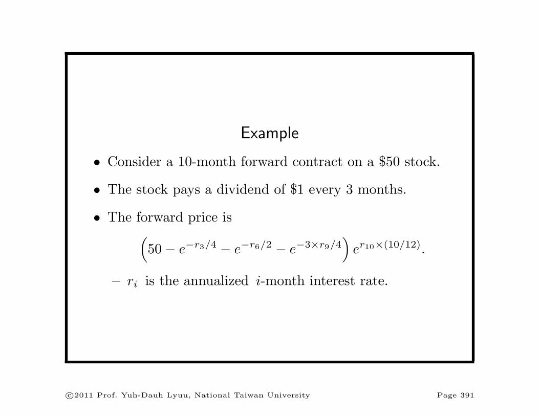
• Consider a 10-month forward contract on a $50 stock.

• The stock pays a dividend of $1 every 3 months.

• The forward price is(50− e−r3/4 − e−r6/2 − e−3×r9/4

)er10×(10/12).

– ri is the annualized i-month interest rate.


Underlying Pays a Continuous Dividend Yield of q

The value of a forward contract at any time prior to T is

f = Se−qτ −Xe−rτ . (34)

• Consider a portfolio of one long forward contract, cashamount Xe−rτ , and a short position in e−qτ units ofthe underlying asset.

• All dividends are paid for by shorting additional units ofthe underlying asset.

• The cash will grow to X at maturity.

• The short position will grow to exactly one unit of theunderlying asset.


Underlying Pays a Continuous Dividend Yield(concluded)

• There is sufficient fund to take delivery of the forwardcontract.

• This offsets the short position.

• Since the value of the portfolio is zero at maturity, itsPV must be zero.

• One consequence of Eq. (34) is that the forward price is

F = Se(r−q) τ . (35)


Futures Contracts vs. Forward Contracts

• They are traded on a central exchange.

• A clearinghouse.

– Credit risk is minimized.

• Futures contracts are standardized instruments.

• Gains and losses are marked to market daily.

– Adjusted at the end of each trading day based on thesettlement price.


Size of a Futures Contract

• The amount of the underlying asset to be deliveredunder the contract.

– 5,000 bushels for the corn futures on the CBT.

– One million U.S. dollars for the Eurodollar futures onthe CME.

• A position can be closed out (or offset) by entering intoa reversing trade to the original one.

• Most futures contracts are closed out in this way ratherthan have the underlying asset delivered.

– Forward contracts are meant for delivery.


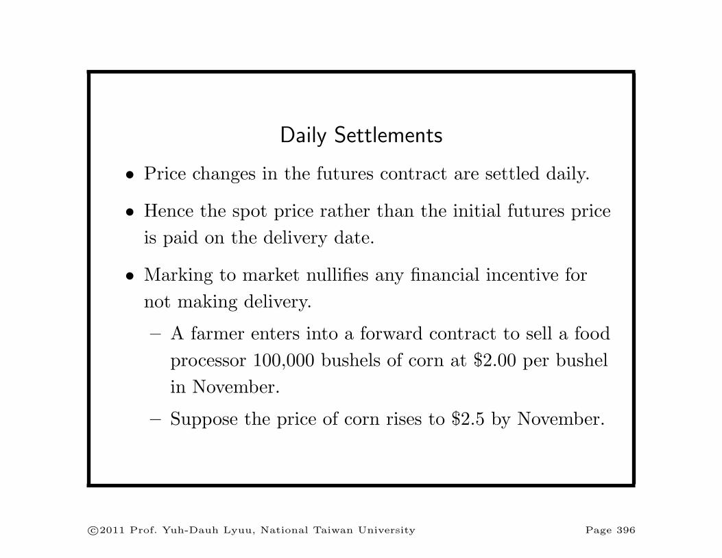
Daily Settlements

• Price changes in the futures contract are settled daily.

• Hence the spot price rather than the initial futures priceis paid on the delivery date.

• Marking to market nullifies any financial incentive fornot making delivery.

– A farmer enters into a forward contract to sell a foodprocessor 100,000 bushels of corn at $2.00 per bushelin November.

– Suppose the price of corn rises to $2.5 by November.


Daily Settlements (concluded)

• (continued)

– The farmer has incentive to sell his harvest in thespot market at $2.5.

– With marking to market, the farmer has transferred$0.5 per bushel from his futures account to that ofthe food processor by November.

– When the farmer makes delivery, he is paid the spotprice, $2.5 per bushel.

– The farmer has little incentive to default.

– The net price remains $2.00 per bushel, the originaldelivery price.


Delivery and Hedging

• Delivery ties the futures price to the spot price.

• On the delivery date, the settlement price of the futurescontract is determined by the spot price.

• Hence, when the delivery period is reached, the futuresprice should be very close to the spot price.a

• Changes in futures prices usually track those in spotprices.

• This makes hedging possible.aBut since early 2006, futures for corn, wheat and soybeans occasion-

ally expired at a price much higher than that day’s spot price.


Daily Cash Flows

• Let Fi denote the futures price at the end of day i.

• The contract’s cash flow on day i is Fi − Fi−1.

• The net cash flow over the life of the contract is

(F1 − F0) + (F2 − F1) + · · ·+ (Fn − Fn−1)

= Fn − F0 = ST − F0.

• A futures contract has the same accumulated payoffST − F0 as a forward contract.

• The actual payoff may differ because of the reinvestmentof daily cash flows and how ST − F0 is distributed.


Forward and Futures Pricesa

• Surprisingly, futures price equals forward price if interestrates are nonstochastic!

– See text for proof.

• This result “justifies” treating a futures contract as if itwere a forward contract, ignoring its marking-to-marketfeature.

aCox, Ingersoll, and Ross (1981).


Remarks

• When interest rates are stochastic, forward and futuresprices are no longer theoretically identical.

– Suppose interest rates are uncertain and futuresprices move in the same direction as interest rates.

– Then futures prices will exceed forward prices.

• For short-term contracts, the differences tend to besmall.

• Unless stated otherwise, assume forward and futuresprices are identical.


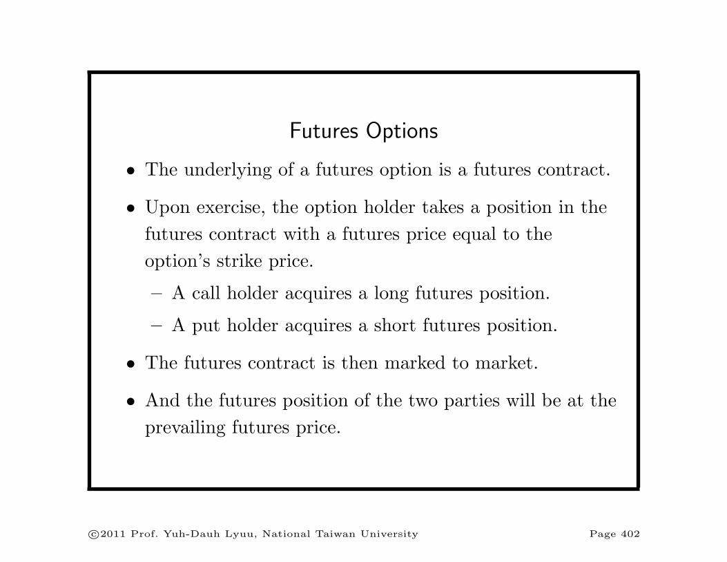
Futures Options

• The underlying of a futures option is a futures contract.

• Upon exercise, the option holder takes a position in thefutures contract with a futures price equal to theoption’s strike price.

– A call holder acquires a long futures position.

– A put holder acquires a short futures position.

• The futures contract is then marked to market.

• And the futures position of the two parties will be at theprevailing futures price.


Futures Options (concluded)

• It works as if the call holder received a futures contractplus cash equivalent to the prevailing futures price Ft

minus the strike price X.

– This futures contract has zero value.

• It works as if the put holder sold a futures contract forthe strike price X minus the prevailing futures price Ft.


Forward Options

• Similar to futures options except that what is deliveredis a forward contract with a delivery price equal to theoption’s strike price.

– Exercising a call forward option results in a longposition in a forward contract.

– Exercising a put forward option results in a shortposition in a forward contract.

• Exercising a forward option incurs no immediate cashflows.


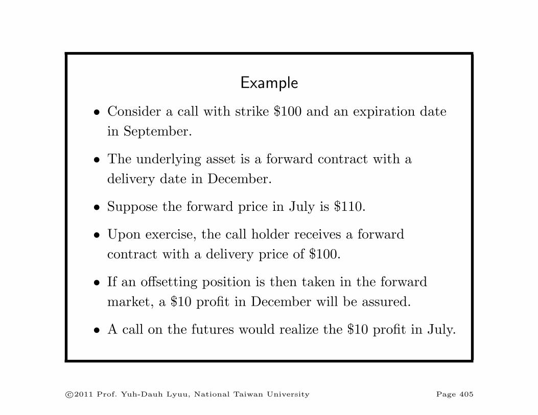
Example

• Consider a call with strike $100 and an expiration datein September.

• The underlying asset is a forward contract with adelivery date in December.

• Suppose the forward price in July is $110.

• Upon exercise, the call holder receives a forwardcontract with a delivery price of $100.

• If an offsetting position is then taken in the forwardmarket, a $10 profit in December will be assured.

• A call on the futures would realize the $10 profit in July.


Some Pricing Relations

• Let delivery take place at time T , the current time be 0,and the option on the futures or forward contract haveexpiration date t (t ≤ T ).

• Assume a constant, positive interest rate.

• Although forward price equals futures price, a forwardoption does not have the same value as a futures option.

• The payoffs of calls at time t are

futures option = max(Ft −X, 0), (37)

forward option = max(Ft −X, 0) e−r(T−t). (38)


Some Pricing Relations (concluded)

• A European futures option is worth the same as thecorresponding European option on the underlying assetif the futures contract has the same maturity as theoptions.

– Futures price equals spot price at maturity.

– This conclusion is independent of the model for thespot price.


Put-Call Parity

The put-call parity is slightly different from the one inEq. (19) on p. 186.

Theorem 11 (1) For European options on futurescontracts, C = P − (X − F ) e−rt. (2) For European optionson forward contracts, C = P − (X − F ) e−rT .

• See text for proof.


Early Exercise and Forward Options

The early exercise feature is not valuable.

Theorem 12 American forward options should not beexercised before expiration as long as the probability of theirending up out of the money is positive.

• See text for proof.

Early exercise may be optimal for American futures optionseven if the underlying asset generates no payouts.

Theorem 13 American futures options may be exercisedoptimally before expiration.


Black Modela

• Formulas for European futures options:

C = Fe−rtN(x)−Xe−rtN(x− σ√

t), (39)

P = Xe−rtN(−x + σ√

t)− Fe−rtN(−x),

where x ≡ ln(F/X)+(σ2/2) t

σ√

t.

• Formulas (39) are related to those for options on a stockpaying a continuous dividend yield.

• In fact, they are exactly Eqs. (25) on p. 274 with thedividend yield q set to the interest rate r and the stockprice S replaced by the futures price F .

aBlack (1976).


Black Model (concluded)

• This observation incidentally proves Theorem 13(p. 409).

• For European forward options, just multiply the aboveformulas by e−r(T−t).

– Forward options differ from futures options by afactor of e−r(T−t) based on Eqs. (37)–(38) on p. 406.


Binomial Model for Forward and Futures Options

• Futures price behaves like a stock paying a continuousdividend yield of r.

– The futures price at time 0 is (p. 386)

F = SerT .

– From Lemma 7 (p. 251), the expected value of S attime ∆t in a risk-neutral economy is

Ser∆t.

– So the expected futures price at time ∆t is

Ser∆ter(T−∆t) = SerT = F.


Binomial Model for Forward and Futures Options(concluded)

• Under the BOPM, the risk-neutral probability for thefutures price is

pf ≡ (1− d)/(u− d)

by Eq. (26) on p. 276.

– The futures price moves from F to Fu withprobability pf and to Fd with probability 1− pf.

• The binomial tree algorithm for forward options isidentical except that Eq. (38) on p. 406 is the payoff.


Spot and Futures Prices under BOPM

• The futures price is related to the spot price viaF = SerT if the underlying asset pays no dividends.

• The stock price moves from S = Fe−rT to

Fue−r(T−∆t) = Suer∆t

with probability pf per period.

• Similarly, the stock price moves from S = Fe−rT to

Sder∆t

with probability 1− pf per period.


Negative Probabilities Revisited

• As 0 < pf < 1, we have 0 < 1− pf < 1 as well.

• The problem of negative risk-neutral probabilities is nowsolved:

– Suppose the stock pays a continuous dividend yieldof q.

– Build the tree for the futures price F of the futurescontract expiring at the same time as the option.

– Calculate S from F at each node viaS = Fe−(r−q)(T−t).

• Of course, this model may not be suitable for pricingbarrier options (why?).


Swaps

• Swaps are agreements between two counterparties toexchange cash flows in the future according to apredetermined formula.

• There are two basic types of swaps: interest rate andcurrency.

• An interest rate swap occurs when two parties exchangeinterest payments periodically.

• Currency swaps are agreements to deliver one currencyagainst another (our focus here).


Currency Swaps

• A currency swap involves two parties to exchange cashflows in different currencies.

• Consider the following fixed rates available to party Aand party B in U.S. dollars and Japanese yen:

Dollars Yen

A DA% YA%

B DB% YB%

• Suppose A wants to take out a fixed-rate loan in yen,and B wants to take out a fixed-rate loan in dollars.


Currency Swaps (continued)

• A straightforward scenario is for A to borrow yen atYA% and B to borrow dollars at DB%.

• But suppose A is relatively more competitive in thedollar market than the yen market.

– That is, YB − YA < DB −DA.

• Consider this alternative arrangement:

– A borrows dollars.

– B borrows yen.

– They enter into a currency swap with a bank as theintermediary.


Currency Swaps (concluded)

• The counterparties exchange principal at the beginningand the end of the life of the swap.

• This act transforms A’s loan into a yen loan and B’s yenloan into a dollar loan.

• The total gain is ((DB −DA)− (YB − YA))%:

– The total interest rate is originally (YA + DB)%.

– The new arrangement has a smaller total rate of(DA + YB)%.

• Transactions will happen only if the gain is distributedso that the cost to each party is less than the original.


Example

• A and B face the following borrowing rates:

Dollars Yen

A 9% 10%

B 12% 11%

• A wants to borrow yen, and B wants to borrow dollars.

• A can borrow yen directly at 10%.

• B can borrow dollars directly at 12%.


Example (continued)

• The rate differential in dollars (3%) is different fromthat in yen (1%).

• So a currency swap with a total saving of 3− 1 = 2% ispossible.

• A is relatively more competitive in the dollar market.

• B is relatively more competitive in the the yen market.


Example (concluded)

• Figure next page shows an arrangement which isbeneficial to all parties involved.

– A effectively borrows yen at 9.5%.

– B borrows dollars at 11.5%.

– The gain is 0.5% for A, 0.5% for B, and, if we treatdollars and yen identically, 1% for the bank.


Party BBankParty A

Dollars 9% Yen 11%

Dollars 9%

Yen 11%Yen 9.5%

Dollars 11.5%


As a Package of Cash Market Instruments

• Assume no default risk.

• Take B on p. 423 as an example.

• The swap is equivalent to a long position in a yen bondpaying 11% annual interest and a short position in adollar bond paying 11.5% annual interest.

• The pricing formula is SPY − PD.

– PD is the dollar bond’s value in dollars.

– PY is the yen bond’s value in yen.

– S is the $/yen spot exchange rate.


As a Package of Cash Market Instruments (concluded)

• The value of a currency swap depends on:

– The term structures of interest rates in the currenciesinvolved.

– The spot exchange rate.

• It has zero value when

SPY = PD.

c©2011 Prof. Yuh-Dauh Lyuu, National Taiwan University 5

Example

• Take a two-year swap on p. 423 with principal amountsof US$1 million and 100 million yen.

• The payments are made once a year.

• The spot exchange rate is 90 yen/$ and the termstructures are flat in both nations—8% in the U.S. and9% in Japan.

• For B, the value of the swap is (in millions of USD)

1

90× (

11× e−0.09 + 11× e−0.09×2 + 111× e−0.09×3)

− (0.115× e−0.08 + 0.115× e−0.08×2 + 1.115× e−0.08×3

)= 0.074.


As a Package of Forward Contracts

• From Eq. (34) on p. 392, the forward contract maturingi years from now has a dollar value of

fi ≡ (SYi) e−qi −Die−ri. (40)

– Yi is the yen inflow at year i.

– S is the $/yen spot exchange rate.

– q is the yen interest rate.

– Di is the dollar outflow at year i.

– r is the dollar interest rate.


As a Package of Forward Contracts (concluded)

• For simplicity, flat term structures were assumed.

• Generalization is straightforward.


Example

• Take the swap in the example on p. 426.

• Every year, B receives 11 million yen and pays 0.115million dollars.

• In addition, at the end of the third year, B receives 100million yen and pays 1 million dollars.

• Each of these transactions represents a forward contract.

• Y1 = Y2 = 11, Y3 = 111, S = 1/90, D1 = D2 = 0.115,D3 = 1.115, q = 0.09, and r = 0.08.

• Plug in these numbers to get f1 + f2 + f3 = 0.074million dollars as before.


Stochastic Processes and Brownian Motion


Of all the intellectual hurdles which the human mindhas confronted and has overcome in the last

fifteen hundred years, the one which seems to meto have been the most amazing in character and

the most stupendous in the scope of itsconsequences is the one relating to

the problem of motion.— Herbert Butterfield (1900–1979)


Stochastic Processes

• A stochastic process

X = {X(t) }

is a time series of random variables.

• X(t) (or Xt) is a random variable for each time t andis usually called the state of the process at time t.

• A realization of X is called a sample path.

• A sample path defines an ordinary function of t.


Stochastic Processes (concluded)

• If the times t form a countable set, X is called adiscrete-time stochastic process or a time series.

• In this case, subscripts rather than parentheses areusually employed, as in

X = {Xn }.

• If the times form a continuum, X is called acontinuous-time stochastic process.


Random Walks

• The binomial model is a random walk in disguise.

• Consider a particle on the integer line, 0,±1,±2, . . . .

• In each time step, it can make one move to the rightwith probability p or one move to the left withprobability 1− p.

– This random walk is symmetric when p = 1/2.

• Connection with the BOPM: The particle’s positiondenotes the total number of up moves minus that ofdown moves up to that time.


20 40 60 80Time

-8

-6

-4

-2

2

4

Position


Random Walk with Drift

Xn = µ + Xn−1 + ξn.

• ξn are independent and identically distributed with zeromean.

• Drift µ is the expected change per period.

• Note that this process is continuous in space.


Martingalesa

• {X(t), t ≥ 0 } is a martingale if E[ |X(t) | ] < ∞ fort ≥ 0 and

E[ X(t) |X(u), 0 ≤ u ≤ s ] = X(s), s ≤ t. (41)

• In the discrete-time setting, a martingale means

E[Xn+1 |X1, X2, . . . , Xn ] = Xn. (42)

• Xn can be interpreted as a gambler’s fortune after thenth gamble.

• Identity (42) then says the expected fortune after the(n + 1)th gamble equals the fortune after the nthgamble regardless of what may have occurred before.

aThe origin of the name is somewhat obscure.


Martingales (concluded)

• A martingale is therefore a notion of fair games.

• Apply the law of iterated conditional expectations toboth sides of Eq. (42) on p. 437 to yield

E[Xn ] = E[ X1 ] (43)

for all n.

• Similarly, E[ X(t) ] = E[ X(0) ] in the continuous-timecase.


Still a Martingale?

• Suppose we replace Eq. (42) on p. 437 with

E[ Xn+1 |Xn ] = Xn.

• It also says past history cannot affect the future.

• But is it equivalent to the original definition (42) onp. 437?a

aContributed by Mr. Hsieh, Chicheng (M9007304) on April 13, 2005.


Still a Martingale? (continued)

• Well, no.a

• Consider this random walk with drift:

Xi =

Xi−1 + ξi, if i is even,

Xi−2, otherwise.

• Above, ξn are random variables with zero mean.aContributed by Mr. Zhang, Ann-Sheng (B89201033) on April 13,

2005.


Still a Martingale? (concluded)

• It is not hard to see that

E[ Xi |Xi−1 ] =

Xi−1, if i is even,

Xi−1, otherwise.

– It is a martingale by the “new” definition.

• But

E[ Xi | . . . , Xi−2, Xi−1 ] =

Xi−1, if i is even,

Xi−2, otherwise.

– It is not a martingale by the original definition.


forward price - 國立臺灣大學lyuu/finance1/2011/20110413.pdf · forward price † the payoﬁ...

Documents