forum for electromagnetic research · pdf filethe state-of-the-art direct digital synthesis...

FORUM FOR ELECTROMAGNETIC RESEARCH METHOD AND APPLICATION TECHNOLOGIES (FERMAT) 1

A Frequency-Modulated Continuous WavePhased Array Marine Radar System

Based on Smart Antenna TechnologyRuey-Bing (Raybeam) Hwang, Yi-Che Tsai, Chun-Fan Chien, Fang-Yao Kuo, Hsien-Tung Huang,

Wei-Hsiung Chen, Cherng-Chyi Hsiao, Chin-Cheng Chuang, Ke-Wen Lin, Yuan-Hao Sun

Abstract—We describe an X-band marine phased-arrayfrequency-modulated continuous-wave (FMCW) radar systembased on the smart antenna technology. Two main features,including the beam-forming and angles-of-arrival (AOA) estima-tion, are presented in this paper. Such a system is composed ofeight subarray antennas arranged linearly, each of which consistsof ten 1-D patch array antennas generating a directional patternalong the vertical plane. The hybrid analog-digital beam-formingscheme was implemented; specifically, the phased local oscillatorwas developed for manipulating the phase angle over the localoscillator rather than over the output X-band signal for trans-mission. Alternatively, by dynamically adjusting the amplitudeand phase of the FMCW signals generated by direct digitalsynthesis (DDS) device, we can also achieve the function of beam-forming. Additionally, the angles-of-arrival of the correlated echosignal scattering by targets are estimated by using the subspacemethod – space smooth multiple signal classification (MUSIC)algorithm. The AOA estimator, which includes the hardware fordown-converting the X-band signals to I/Q baseband and thesoftware for algorithm implementation, has been deployed. Themeasurements for range detection, angles of arrival estimation,and beam-forming has been carried out in this research work.

Keywords—FMCW, smart antenna system, phased-array system,angle-of-arrival estimation, beam-forming technique.

I. INTRODUCTION

FMCW radar has been widely used in civilian and mili-tary applications of surveillance, tracking, precision ranging,medical diagnosis, and automotive collision avoidance [1], [2],[3], [4]. FMCW radars transmit broadband linear FM signalin a periodic swept time. Radar range resolution is inverselyproportional to the FM bandwidth. The period of the swepttime is longer than the round-trip time of the most distanttarget. FMCW radar receiver is typically a simple homodynearchitecture that mixes the target echo with a replica of thetransmit waveform. The beat frequencies can be determinedthrough the fast Fourier Transform (FFT); the target rangesas well as speed can be obtained accordingly. As far as themixing process is concerned, the linearity of the linear FM

R. -B. Hwang, Y. -C. Tsai, C. -F. Chien, F. -Y. Kuo, H. -T. Huang, K. -W.Lin, C. -C. Hsiao, C. -C. Chung, and Y. -H. Sun are with the ECE Department,National Chiao Tung University, Hsinchu, 30010, Taiwan. W.-H. Chen is withthe ZyFlex Technology, Hsinchu 30075, Taiwan. Corresponding author: Prof.Ruey-Bing Hwang with his email: [email protected]. This researchis supported in part by the Ministry of Science and Technology, Taiwan underthe contract:NSC 101-2221-E-009-097-MY2

signals is an important factor affecting the system performance.Specifically, the non-linearity of the FMCW waveform intro-duces extra spurious beating signals, enabling the occurrenceof false alarms. The state-of-the-art direct digital synthesis(DDS) technique is now available to generate linear FM signalsthat simultaneously have acceptable linearity for required rangeresolution and spurious rejection.

Regarding the radar transmitter, the solid-state power am-plifier (SSPA) is frequently used now as a power transmitterfor some short range applications. Because the average trans-mitting power of SSPA, the FMCW radar can be comparableto that of a high peak-power and low duty-cycle pulse radar.Therefore, some short range pulse radars using cavity-resonantmagnetron may gradually be replaced by SSPA FMCW radars.One type of FMCW radar uses a single antenna and a circulatorto transmit and receive RF signals simultaneously. This typeof FMCW radar always needs a self-cancellation circuit infront of the receiver low-noise amplifier (LNA) to suppress theself-interference. Another useful method to suppress the self-interference is to add metallic baffles outside the transmittingand receiving antennas for enhancing the isolation betweenthem [5].

Beam-forming (or spatial filtering) technique entails anapplication of the phase weights to the element antennas ofan array. The angular spectrum of the directivity pattern canexhibit constructive interference at particular (desired) anglesbut destructive interference at the other angles. For the radarsystem exploiting a mechanically scanned antenna, the highdirectivity beam pattern is scanned by using a gimbal-typeservo. However, the phased-array radar system can steer itsmain beam with high directivity by using the beam-formingtechnique. The dynamic phased array has higher frame ratesand is more robust in comparison to the antennas with me-chanical beam steering. The beam-forming technique has beenextensively investigated using schemes that use analog phaseshifters and digital signal processing [6], [7]. From the viewpoint of radar receivers, beam-forming can improve the signal-to-noise ratio by combining the signals coherently (weighteddelay-and-sum), enabling the accuracy enhancement in targetrange- and direction- detection. On the other hand, beam-forming implemented in a transceiver is equivalent to spatialpower combining, which coherently combines each of thesignal radiating from the element antenna of an array. In ourresearch work, the beam-forming is merely applied in the radartransmitter for improving the gain of the transmitter.


It should be pointed out that the calibration process is criticalto synthesizing a desired array pattern achieved by realizing thedesired amplitude and phase distributions over the entire array.Some calibration techniques empoly the antenna pattern, andmodeling methods which include mutual coupling effects [8],[9] for this purpose. In this paper, calibration is implementedby tapping each transmitter output and down-converting intoI/Q baseband to calculate the correction factors to the weights.

Array radars usually incorporate angle-of-arrival (AOA) es-timation algorithms to search multiple targets. Eigen-structuremethod is widely used for AOA estimation in noisy environ-ments [10]. A variety of AOA estimation algorithms are avail-able for phased array systems; for example, Bartlet, Capon,Min-norm, MUSIC and ESPRIT [11], [12], [13], [14], [15].Among these algorithms, MUSIC provides high resolution aswell as accuracy, and is widely implemented in phased arrayradar systems. The Eigen-structure AOA algorithm forms acorrelation matrix from a number of samples (snapshots) ofthe array elements, and then decomposes the correlation matrixinto signal eigen-space and noise eigen-space. Based on theorthogonal property of these two sub-spaces, the angles of theincoming plane waves can be estimated through a search ofthe peaks of the pseudo-spectrum. The number of sources inthe system is usually limited to the number of array elements.Unfortunately, the traditional MUSIC algorithm cannot handlecorrelated signals that typically arise in a radar scenario, andreduce the rank of the correlation matrix. Smoothed MUSICalgorithm was reported to be able to remove the correlation bycalculating the smoothed correlation matrix, obtained by usingthe arithmetic mean of the correlation matrices correspondingto the overlapped subarrays subdivided from the original array[16], [17], [18].

This paper is organized as follows. Section II presents theprinciple of the FMCW radar, while Section III describesthe phased-array FMCW radar architecture. Next, the hybridanalog-digital beamformer is introduced in Section IV. SectionV discusses the angle-of-arrival estimation algorithm and itshardware implementation. Section VI presents the details ofradar performance evaluation, angle and range detection, andthose of the range resolution measurements. Finally, someconcluding remarks are presented in Section VII to summarizethe paper.

II. PRINCIPLE OF AN FMCW RADAR

Figure 1 shows the function block diagram of an FMCWradar system, including the transmitter, the receiver and twoisolated high-gain antennas. To obtain a highly linear FMCWsweep signal, we use a DDS to generate a linear up-down chirpFMCW signal with a swept frequency bandwidth B, which iscentered at fc, and has a sweep time Ts. The time-varyingFMCW signal is generally written as:

S(t) = A cos

(2πfct± π

B

Tst2)

(1)

where fc is the carrier frequency and A is the amplitude ofthe FMCW signal. Note that in our system, B and Ts are 50MHz (from 175 MHz to 225 MHz) and 0.25 ms, respectively.

DDS LNA

Phased LO

LNA Power Amp.

LNALPF

TX Ant

RX Ant

DAQ System and PC

Waveform Generator Up Converter

Down Converter

Power Amp.

DAQPC

BPF

BPF

I

Q LNA

Phase Calibration

LNA

Fig. 1. Function block diagram of a typical FMCW radar system.

Sweep time

Sweep frequency

TransmitterReceiver

sT

B

δt

δf

Fig. 2. The relation between the sweep frequency and sweep time for thetransmitted and received FMCW signals.

Note that the plus sign in (1) represents the up-chirp signal,whereas the minus sign is associated with the down-chirp one.

As shown in Fig. 1, the baseband signal is up-convertedto X-band centered at 9410 MHz by a 9210 MHz STALO(stable local oscillator). Following the up-conversion mixer isa bandpass filter to remove the lower sideband and unwantedsignals such as the leakage from the LO. The X-band FMCWsignal goes though a bandpass filter and a power amplifier,and is then delivered to a transmitting antenna for radiating.The echo signal from the target is received by the receivingantenna and is processed through a bandpass filter and a low-noise amplifier. Additionally, a homodyne receiver architectureis used; an IQ demodulator is used to convert the X-band echosignal directly to I and Q baseband through a local oscillatorsignal, which is a replica coupled from the transmitter (after thepower amplifier) via a directional coupler. After sampling theI and Q data by using a data acquisition (DAQ) system, whichis controlled by a personal computer system, we obtain thetarget information, including the range and speed of a movingtarget.

As shown in Fig. 2, the received waveform (blue) is simplya delay replica of the transmitted one. The frequency shiftbetween the transmitted and received waveforms, denoted asδf (beat frequency), can be directly read from the figure as faras the time delay is specified, which is prescribed as δt. Thus,


the relation between the delay time and beat frequency can bereadily obtained as:

δt =δfTsB

(2)

Note that δT is the round-trip time for the electromagneticwave launched from the transmitter, reflected by the target, andreturned to the receiver. The distance between the radar andtarget is then determined by:

R =CδfTs

2B(3)

, where C is the speed of light in vacuum.Furthermore, as mentioned previously the beat frequency

between the transmitted and received signals can be directlyobtained through a direct-conversion (zero-IF) receiver. There-fore, a multitude of pseudo-beat-frequencies will be exhibtedif nonlinearities are present. Additionally, the range resolution(∆R) of the FMCW radar system can be determined by usingthe equation below:

∆R =C

2B(4)

Thus, an increase in the sweep bandwidth (B) would en-hance the range resolution for an FMCW radar system.

III. PHASED-ARRAY FMCW RADAR ARCHITECTURE

In this work, we extend a commonly used single channelFMCW radar to a phased-array system containing 8 channels,each of which consists of a transmitter, a receiver, and subarrayantennas. The 8 subarray antennas are arranged in a one-dimensional periodic nature with a period of 15.6 mm alongthe horizontal direction. The architecture, which is comprisedof a transmitter and an array of 8 receivers was developed forthe AOA detection. For this operating mode, only the anglesof echo signals are detected. Once the angles of arrival hasbeen determined, the beamformer, consisting of array of 8transmitters and a receiver, is exploited to detect the rangewhile scanning in the vicinity of the angles of arrival. For thesingle channel transmitter or receiver, their system architec-tures are the same as those of the traditionally ones. The maindifference stems from the dynamic control and calibration ofthe amplitude as well as the phase angle on each channel.In this section, we will introduce the system architecture ofan FMCW radar transceiver, including the active and passivecomponents and antennas.

A typical FMCW radar system, shown in Fig. 1, contains atransmitter, a receiver, and two antennas for transmitting andreceiving signals. The design of an FMCW radar begins withthe link-budget calculation, which is dominated by the signal-to-noise ratio (SNR) of a receiver. The signal-to-noise ratio ofa radar receiver can be evaluated by using the formula givenbelow:

SNR =PtGtGrλ

2σ

(4π)3kBTBFnLsR4(5)

, where Pt is the transmitted power; Gt(Gr) is the transmitting(receiving) antenna gain; λ is the operating wavelength; σ isthe target radar cross section; kB is the Boltzmann’s constantequal to 1.38e−23Joule/oK; T is the temperature in oK; Bis the Fast Fourier Transform (FFT) resolution bandwidth; Fnis the noise figure of the receiver; Ls is the system loss; andR is the range between the target and radar. It is well knownthat not only the performance of range detection but also thatof the angle-of-arrival detection is strongly related to SNR ofeach receiver. Consequently, SNR is the most critical issue inan FMCW radar receiver design.

Additionally, the phase noise of the stable local oscillator isan important factor affecting the SNR of a radar system. Let theminimum detectable signal-to-noise ratio at a radar receiver –be denoted as SNR. The parameter ∆S is the power difference(in dB) between the unwanted and wanted signals, where theseparation in frequency is denoted by δf . The unwanted signaldefined here may be the result of direct coupling from thetransmitter or due to reflection from nearby scatterers. Thefollowing equation can be used to determine the phase noisespecification of a local oscillator.

S∆φ = −(SNR+ ∆S + 10 log10BW ) (6)

, where BW represents the FFT resolution bandwidth in Hz;the unit of the phase noise is dBc/Hz. For example, if weassume that ∆S = 60 dB, SNR = 12 dB, the FFT resolutionbandwidth is 1 KHz, and ∆f = 1 MHz, then the phase noisewill be −(12 + 60 + 10 log10 1000) = −102 dBc/Hz at 1MHz away from the center of the unwanted signal.

In a commonly used phased array system, a phase shifteris used to manipulate the phase angle of each RF signaldelivered to the element antenna. Therefore, for a signalwhich has a wide bandwidth, the frequency response of aphase shifter must be taken into account and a sophisticatedfeedback control for phase calibration is absolutely essential.To overcome this drawback, we manipulate the phase angleover the single frequency generated by the STALO (stable localoscillator) rather than directly on the broadband RF signal. Inthe following section, the design of the phased local oscillatorwill be described.

A. Phased STALO (stable local oscillator)The phased STALO is a phase adjustable stable local

oscillator. A voltage-controlled oscillator (Mini-Circuits MOS-2360-119+) operating at 2302.5 MHz is connected to a voltage-controlled phase shifter (Mini-Circuits JSPHS-2484+). It isfollowed by a multiplier made of an Infineon Silicon Ger-manium RF transistor, operating in the non-linear region, toobtain the harmonics of the input signal. A subsequent high-Qbandpass filter, which will be described later on, selects thedesired harmonic frequency, which is, 9210 MHz, and filtersout the other harmonics and fundamental from the output.The phase noise of the VCO at 2302.5 MHz is -122 dBc/Hzat 1 MHz offset. Through the ×4 multiplier, its phase noisedegrades to -110 dBc/Hz at 1 MHz offset. However, it is stillacceptable according to the rule of thumb mentioned in theprevious section.


B. Passive componentsThe microwave band-pass filter (BPF) is an essential com-

ponent for removing the unwanted signals and allowing the de-sired signals to pass. As far as a band-pass filter is concerned,we need to take three factors into account, namely the returnloss, the insertion loss, and the variation of the group delayin the passband. Additionally, to provide a sufficient imagerejection for the signal through a nonlinear device, frequencyselectivity is also an important factor to be considered forbandpass filter design. To enhance the frequency selectivity,many BPF stages are cascaded; however, the insertion loss isthen increased dramatically. Therefore, the design tradeoff isalways an issue, particularly for the receiver design (systemloss in the SNR equation in (5)).

1) Six-pole BPF: The six-pole Chebyshev bandpass filterwith a 0.01-dB ripple level was designed to suppress the lowerside-band signal from 8985 MHz to 9035 MHz, generated byan up-conversion mixer in the transmitter, as well as by the LOleakage. Since the LO (at 9210 MHz) and the upper side-band(from 9385 MHz to 9435 MHz) signals are very close to eachother, a BPF with high frequency selectivity is required. Herea six-pole BPF with the center frequency and bandwidth of9500 MHz and 320 MHz was synthesized based on the designrule [19], [20], with the coupling coefficients and the externalquality factor given below:

M12 = M56 = 0.033M23 = M45 = 0.022M34 = 0.021Qext = 23.19

(7)

0.6 0.8 1.0 1.2 1.4 1.6 1.80.03

0.04

0.05

0.06

0.07

0.08

0.09

c = 0.52 mm c = 0.86 mm

s (mm)

Coup

ling

Coef

ficie

nt

0.020

0.025

0.030

0.035

0.040

0.045

0.050

Cou

plin

g Co

effic

ient

Fig. 3. Simulated coupling coefficients versus the distances between theresonators.

Here, an open-loop resonator is taken as the basic unitcell for the BPF design. The open-loop resonator has a half-wavelength perimeter at a center frequency of 9500 MHz asshown in Fig. 3. The resonator was printed on a microwavesubstrate with a relative dielectric constant of 3.38, loss tangentof 0.0027, and a thickness of 32 mil. The coupling coefficientfor various separation distances between the two resonatorscan be extracted from numerical simulations by using theCST Microwave Studio [25]. Using Fig. 3, and the coupling

coefficients given in (7), we may determine the separationdistances between the two adjacent resonators that are givenby: d34 = 1.65 mm, d23 = d45 = 1.59 mm, d12 = d56 = 1.28mm, df = 0.51 mm, the other relevant parameters are c = 0.86mm and Lf = 4.43 mm. The physical circuit layout is shownin Fig. 4.

Fig. 5 shows the measured results with the photograph ofthe six-pole bandpass filter attached. The size of the filter is22.9 mm by 5.9 mm, i.e., 0.73 λg by 0.19 λg , where λg isthe guided-wave wavelength at the center frequency. Note thata 35 dB suppression for the lower sideband signal has beenachieved. Moreover, the reduction of LO leakage at 9210 MHzis up to 25 dB.

d34

d23

d12

d45

d56

c

df

df

LfLf

Fig. 4. Circuit layout of the Six-pole band-pass filter at a center frequencyand bandwidth of 9500 MHz and 320 MHz.

8.4 8.8 9.2 9.6 10.0 10.4

-40

-30

-20

-10

0

S-pa

ram

eter

(dB)

Frequency(GHz)

S11 S21 S22 S12

Fig. 5. Measured results of the six-pole bandpass filter.

2) Four-pole BPF: The next BPF to be presented is used forthe purpose of selecting the fourth harmonic of the input signalvia the ×4 multiplier. The four-pole Chebyshev bandpass filterwith a 0.01 dB ripple level was employed (see Fig. 6). Thecenter frequency of the bandpass filter is set to 9210 MHz, withthe bandwidth of 500 MHz. The coupling coefficients and theexternal quality factor corresponding to the design specificationare given below:

M12 = M34 = 0.058M23 = 0.043Qext = 13.12

(8)

Repeating the design procedure that we have presentedpreviously, the distance between the adjacent resonators canbe determined. They are: d23 = 1.1 mm, d12 = d34 = 0.94mm, df = 0.4 mm, c = 0.52 mm, and Lf = 4.5 mm. Themeasured S-parameters and the photograph of the four-poleband-pass filter was shown in Fig. 7. The length of the filter


d12 d34

df

df

LfLf

d23

c

Fig. 6. Four-pole bandpass filter at a center frequency 9.21 GHz.

8.0 8.5 9.0 9.5 10.0 10.5-40

-30

-20

-10

0

S-pa

ram

eter

(dB)

Frequency(GHz)

S11 S21 S22 S12

Fig. 7. Measured S-parameters and the photograph of the four-pole bandpassfilter.

is 13.7 mm and its width is 6.4 mm, i.e., its dimensions inwavelength are 0.42 λg by 0.20 λg , where λg is the guidedwavelength on the substrate at 9210 MHz.

3) Bandpass Filter with SIRs at a Center Frequency of2302.5 MHz: To filter out the spurious harmonics generated bythe VCO, a BPF based on the stepped-impedance resonators(SIRs) [21], [22], [23] was designed to achieve wide bandrejection for the unwanted harmonics. The center frequency ofthe BPF was designed to be 2302.5 MHz, with a bandwidth 50MHz. The impedance ratio (Z2/Z1) R = 0.3 and the lengthratio (θ2/(θ1+θ2)) u = 0.7 were chosen to extend the rejectionband to 3f0. Figure 9 shows the measured results with thestructure attached. The structure parameters of the BPF are:s = 1.3 mm, L1 = 2.8 mm, L2 = 6.9 mm, W1 = 0.3 mm andW2 = 6 mm. The size of the filter is 19.4 mm by 13.3 mm,i.e., 0.15 λg by 0.10 λg , where λg is the guided wavelengthat 2302.5 MHz. From the measured result shown in Fig. 9,the rejection bands was extended up to 7 GHz for a 17 dBattenuation.

C. Active components

The active components comprise of a low-noise amplifier, apower amplifier, and a voltage-controlled oscillator. The outputP1dB is 34 dBm at 9410 MHz, with a gain of 31.5 dB for thepower amplifier (Hittite HMC-952). The output P1dB is 18dBm at 9410 MHz, with the noise figure of 4.4 dB for the low-noise amplifier (Mini Circuit AVA-183A+). The output powerof the VCO (Mini Circuit ZX95-2490+) is 13.1 dBm at 2302.5MHz.

s

L2 ( 2)2L1

(2 1)

Z2

W1

W2

Z1

Fig. 8. Bandpass filter with SIRs at a center frequency 2302.5 MHz.

1 2 3 4 5 6 7-40

-30

-20

-10

0

S-pa

ram

eter

(dB)

Frequency(GHz)

S11 S21 S22 S12

Fig. 9. Measured S-parameters and the photograph of the SIRs basedbandpass filter.

D. Array antennas

The array antenna used in the beamformer and AOA esti-mator is comprised of 8 subarrays, each containing a uniformlinear array with 10 microstrip antennas, as shown in Fig. 10.The antenna array is implemented on a microwave dielectricsubstrate (RO4003) whose thickness is 0.8mm; the photo ofthe array antenna is shown in Fig. 10. The distance betweenthe two adjacent subarrays is 15.6 mm. The simulated andmeasured reflection coefficient (S11 in dB) of each subarrayantenna is shown in Fig. 11. The measured impedance band-width for S11 = −15dB is from 9350 MHz to 9520 MHz. Asimulation of the radiation angle of the main beam of the singlesubarray showed less than 1.5 degrees of angular variation dueto frequency scan from 9350 MHz to 9550 MHz. Figure 12and 13 show the simulated and measured radiation patternsof each subarray antenna at 9410 MHz in the x–z plane (H-plane) and y–z (E-plane) plane, respectively. Fig. 12 showsthat the measured antenna gain, the half-power beam-width,and the side-lobe level are 16 dBi, 9o, and -15 dB, respectively.The half-power beam-width and the side-lobe level on the y–zplane were 98◦ and -13.5 dB, respectively. Due to the angle-of-arrival application, a wide field-of-view is needed for eachsubarray in the y–z plane. It is apparent that generally theagreement between the measurement and simulation results is


good.

x

y

z

Fig. 10. Photograph of the array antennas consisting of 8 subarray antennasmade of 1D patches array; the x-axis is along the 1D micro-strip array andthe y-axis is along the direction of SMA connectors array.

9 9.2 9.4 9.6 9.8Frequency (GHz)

-30

-25

-20

-15

-10

-5

0

S 11 (

dB)

SimulationMeasurement

Fig. 11. Measured S11 of the subarray antenna (1D patches array).

IV. HYBRID ANALOG-DIGITAL BEAMFORMER

A. System architecture of the beam-forming networkFigure 14 shows the system block of the beam-former

consisting of an array with 8 transmitters, each of whichconverts a linear FM from IF (from 175 MHz to 225 MHz)to X-band, centered at 9410 MHz. Only a single receiveris presented in the figure. The aforementioned phased localoscillator was implemented in the design to serve as an analogbeam-former. The linear FM signal generated by the directdigital synthesizer (two pieces of AD9959) can provide 8independent channel signals, if necessary, with programmablephase angle and amplitude, and the digital beam-forming canbe achieved by using this system. Each of the transmitters hasan architecture similar to the single channel FMCW described

030

60

90

120

150180

210

240

270

300

330

-40 -20 0 20


Fig. 12. Simulated and Measured radiation pattern on the x–z plane (H-plane)of the antenna shown in Fig. 10.

030

60

90

120

150180

210

240

270

300

330

-40 -20 0 20


Fig. 13. Simulated and Measured radiation pattern on the y–z plane (E-plane)of the antenna shown in Fig. 10.

previously. To maintain the same phase angle among the eightphased local oscillators, the sinusoidal signal of 2302.5 MHzVCO is fed into a 1-to-8 power divider based on the Wilkin-son architecture. The phased local oscillator while operatingtogether with the phase shifter, frequency multipliers, band-pass filters and low-noise amplifiers, has the output power of+7 dBm and phase noise of -110 dBc/Hz at 1 MHz offset from9210 MHz carrier frequency. Specifically, for the purpose ofphase calibration, some of the X-band signal in each channel iscoupled (through a T-junction SMA connector) and convertedinto I/Q baseband through an IQ demodulator to measure theirphase angle and amplitude. In this manner, we can calibratethe phase angle of each channel by adjusting the angle of eachof the voltage-controlled phase shifter.


+5 dBm

+9 dBm

0 dBm

+7 dBm

+6 dBm

-10 dBm

0 dBm

-3 dBm

+7 dBm

-12 dBm

-2 dBm

-10 dBm

+0.2 dBm

-3.5 dBm

+23.1dBm

LNA

ChipBPF

Phaseshifter

Multiplier

LNA

LNA

Four-poleBPF

Mixer

LNA

Six-poleBPF

LNA

1-to-2SMA

Adapter

PA

Transmitted Antenna

-14 dBm

-1 dBm

-4 dBm

+7 dBm

I/QMixer

Received Antenna

Four-poleBPF

LNA

LNA

Four-poleBPF

Mixer

Fig. 14. System block diagram of the beamformer consisting of 8 FMCWtransmitters array.

Fig. 15. Photo of the beamformer module.

B. Radiation pattern measurement of the beamformer plussubarray antennas

Figures 16 and 17 show the simulated and measured radi-ation patterns for the phased-array antenna after the analogbeam-forming. Altering the progressive phase delay angleamong the phased local oscillators swings the main beampattern. The progressive phase delay angle corresponding toeach pattern is indicated in the legend. Each of the measuredpattern can generally agree with the simulated one except forthe sidelobe level. It is conjectured that the imperfect taperingover the amplitude distribution of the subarrays results in highsidelobe levels. However, the situation can be improved byusing digital beam-forming technology and letting the DDS

-60 -30 0 30 60Theta (deg.)

-20

-15

-10

-5

0

Am

plitu

de (d

B)

-90 deg.-60 deg.-30 deg.0 deg.30 deg.60 deg.90 deg.

Fig. 16. Simulated radiation pattern with beam-forming.

-60 -30 0 30 60Theta(deg.)

-20

-15

-10

-5

0

Am

plitu

de(d

B)

-90 deg.-60 deg.-30 deg.0 deg30 deg.60 deg.90 deg.

Fig. 17. Measured radiation pattern with beam-forming .

manipulate the amplitude and phase of the IF FMCW signal.Additionally, the measured (simulated) main beam angles are28o(30o), 18o(20o), 10o(10o), 0o(0o), -9o(-10o), -18o(-20o),and -29o(-30o), respectively. The measured 3 dB beam-widthis around 13o, on average.

V. ANGLE-OF-ARRIVAL ESTIMATOR

A. Multiple Signal Classification: MUSIC

An angle-of-arrival estimation algorithm was developed toestimate the direction of the incoming signals through pro-cessing the data received by each of the array antennas. Incomparison with the classical methods, which first computea spatial spectrum and then estimate the angles of arrivalby searching the local maxima of the spectrum, the multiplesignal classification (MUSIC) algorithm can achieve a higherangular resolution via the subspace method. The mathematicalformulation of the MUSIC algorithm is introduced as follows.


Assume an 1-D antenna array with N elements that arearranged along the y-axis with a spacing d. Let us assume thatthere are M (M<N ) incident electromagnetic waves arrivingfrom different angles. First of all, let us consider the casewhere the incident waves may have different angles alongthe elevation direction (θ), but have the same azimuthal angle(φ), which is set to zero. Therefore, the received signal ateach of the antennas, contributed by the M incident waves, isexpressed as:

xn(k) = ξn(k) +

M∑i=1

si(k)eikond sin θi (9)

with the index k representing the kth snapshot (or sample).The parameter ξn(k) is the noise amplitude received by the

nth antenna. The parameter si(k) is the amplitude of the ithincident wave, which is a complex number in general. Wecollect the received signals at each of the antenna and arrangethem in a column vector, which is written as follows:

x(k) = As(k) + ξ(k) (10)

The matrix A has the size N×M with its jth column a(θj)representing the steering vector of the jth signal with theincident angle θj , written below:

a(θj) = (1 eikod sin θj ei2kod sin θj ...ei(N−1)kod sin θj )T (11)

, where j ranges from 1 to M .The column vector s has the dimension M×1, and repre-

sents the incoming signals. The quantity ξ in (10) is a measureof the white Gaussian noise received by each antenna with thesize N×1.

Here, the noise in each channel is supposed to be highlyuncorrelated, enabling us to diagonalize the correlation matrix.Consequently, the correlation matrix of x(k) can be written as:

Rxx = E[x xH ] = ARssAH +Rnn (12)

, where H is the Hermitian operator (conjugate transpose), andE is the statistical average (expected value). The quantitiesRss and Rnn are the source and noise correlation matrices,respectively, and are defined as follows:

Rss = E[s sH ] (13)

Rnn = E[ξ ξH ] = σ2I (14)

The matrix Rxx has M eigenvectors associated with thevj signals with j=1,2,3,...M , and it has N−M eigenvectorsrelated to the noise. We can construct a new subspace by usingthe N−M noise eigenvectors, and write it as follows:

Vnoise = [vM+1 vM+2...vN ] (15)

It is possible to prove that the noise subspace eigenvector in(15) is orthogonal to the steering matrix in (11). Moreover, the

pseudo-spectrum Ppseudo (θ) defined by the MUSIC argorithmcan be written as:

Ppseudo(θ) =1∑N

m=M+1 | AH(θ)vm |2(16)

Owing to the orthogonality between the signal steering andnoise vectors, the denominator in (16) becomes zero when θcorresponds to a signal direction. Therefore, there would be Mpeaks in the pseudo-spectrum distribution, which correspondto the directions of arrival of the signal.

B. Spatial Smooth MUSICThe traditionally used MUSIC assumes that all arrival sig-

nals are uncorrelated (the signal correlation matrix in (13) is adiagonal matrix). In the radar detection scenario, the scatteringwaves are indeed correlated because they oringinate from thetransmitting antenna. The correlation reduces the rank of thesignal correlation matrix in (13), causing the number of noiseeigenvectors to be greater than N−M .

To overcome this problem, the spatial smoothing MUSICalgorithm is employed. First, the original array is subdividedinto 5 overlapped subarrays, each with 4 elements. For ex-ample, the first subarray contains the antennas (1, 2, 3, 4); thesecond one includes (2, 3, 4, 5); the third one is (3, 4, 5, 6);the fourth one is (4, 5, 6, 7); and the last one is (5, 6, 7, 8).The correlation matrix corresponding to each subarray can beobtained and denoted by Rj , whose dimensions are 4 × 4,where j varies from 1 to 5. The MUSIC algorithm is thenapplied for the smoothed correlated matrix, given below:

Rsmooth =1

5

j=5∑j=1

Rj (17)

The matrix Rsmooth above becomes full-rank once again.Consequently, the above formulation can detect the arrivalangles up to 4 correlated signals.

C. AOA Estimator ArchitectureThe system architecture for implementing the MU-

SIC/smooth MUSIC is shown in Fig. 18. The photo of thefabricated AOA estimator is shown in Fig. 19. Recall thatthe receiving antenna was shown earlier in Fig. 10. For eachof the subarrays, the main beamwidth is narrower along thevertical direction, whereas the beamwidth along the horizontaldirection is wider. The receiving antenna is connected to alow-noise amplifier and a band-pass filter. Furthermore, thereceived signal is converted into the baseband I and Q bybeating it with that of the local oscillator (the received signalis a complex number). The baseband signals of each channelcan be further sampled by using a data acquisition system.The arrival angles of the correlated signals can be estimatedby using the spatial smoothing MUSIC algorithm describedpreviously. It is worth mentioning that the calibration mustbe carried out initially to equalize the phases and amplitudesamong the eight channels. We may feed each channel by anin-phase signal to calibrate their amplitudes and phases at their


Signal 1

. . . . . . . . . . . .

LOLO LO

DAQ

. . . . . .

PC

LO

LO

x

y

z

I Q I Q I Q

#1 #2 #8

Signal 2Signal 3

Signal 4

Fig. 18. System block diagram of an AOA estimator.

Fig. 19. Photo of the module of AOA estimator.

baseband frequencies after their down-conversion. Specifically,the weighting factor of each channel is prescribed at baseband.

Figures 20 and 21 show the distribution of the pseudo spec-trum against the incident angle θ, derived by using the MUSICand spatially smoothed MUSIC algorithms, respectively. Thethree correlated signals have the same amplitude but differ-ent prescribed incident angles, namely 52o, 33o, and −10o.Apparently, in Fig. 20, the commonly used MUSIC algorithmcannot handle the correlated signals; however, the spatiallysmoothed MUSIC can correctly estimate the three incidentangles. The figures were obtained via computer simulation ofthe following example. We will demonstrate the use of the

-80 -40 0 40 800

1

2

3

4

5

6

Spat

ial S

pect

rum

(dB

)

Direction of Arrival (degree)

Fig. 20. Pseudo spectrum computed by traditionally used MUSIC

-80 -40 0 40 80

0

10

20

30

40

Spat

ial S

pect

rum

(dB)

Direction of Arrival (degree)Fig. 21. Pseudo spectrum computed by smoothed MUSIC

measured results obtained by processing the data through ourhardware and software systems.

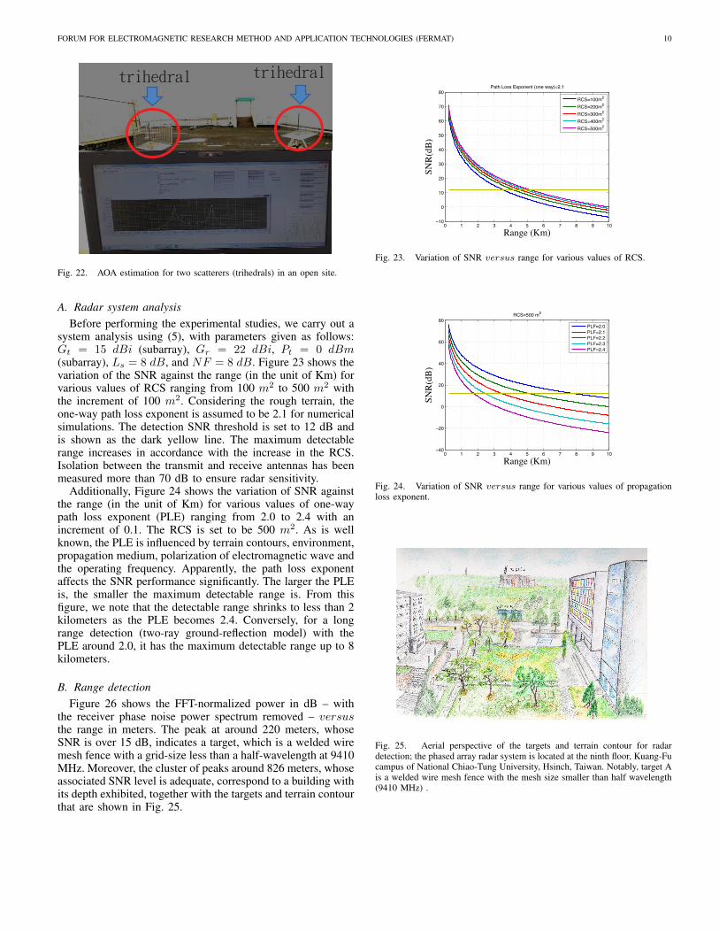
Figure 22 shows the measured results and the testing envi-ronment for the AOA estimation. Two trihedrals were placed infront of the receiving arrays, consisting of an 8 1-D patch array– the receiver architecture is shown in Fig. 18. A transmittingantenna, whose field-of-view is able to cover the two trihedrals,is taken as the illuminator, enabling the echo signals receivedby the array antennas. We employ the trihedral because its RCSis less sensitive to the variation of the incident angle withincertain range of the angular spectrum. It is obvious from theresult shown in this figure that the two targets can be correctlyidentified through our AOA estimator in a complex outdoorenvironment.

VI. RADAR PERFORMANCE EVALUATION

In the previous sections, we have discussed the theoreticaland experimental studies of the FMCW radar transmitter, re-ceiver, beamformer, AOA estimator and phased array antennas.In this section, we focus on the performance evaluation of theFMCW radar system incorporating the phased array system.Specifically, we demonstrate the detection of the range andazimuth angle of the echo signals reflecting from targets toevaluate the performance of the radar system. Additionally,the assessment of range resolution is also carried out by usingthe radar target simulator.


Fig. 22. AOA estimation for two scatterers (trihedrals) in an open site.

A. Radar system analysisBefore performing the experimental studies, we carry out a

system analysis using (5), with parameters given as follows:Gt = 15 dBi (subarray), Gr = 22 dBi, Pt = 0 dBm(subarray), Ls = 8 dB, and NF = 8 dB. Figure 23 shows thevariation of the SNR against the range (in the unit of Km) forvarious values of RCS ranging from 100 m2 to 500 m2 withthe increment of 100 m2. Considering the rough terrain, theone-way path loss exponent is assumed to be 2.1 for numericalsimulations. The detection SNR threshold is set to 12 dB andis shown as the dark yellow line. The maximum detectablerange increases in accordance with the increase in the RCS.Isolation between the transmit and receive antennas has beenmeasured more than 70 dB to ensure radar sensitivity.

Additionally, Figure 24 shows the variation of SNR againstthe range (in the unit of Km) for various values of one-waypath loss exponent (PLE) ranging from 2.0 to 2.4 with anincrement of 0.1. The RCS is set to be 500 m2. As is wellknown, the PLE is influenced by terrain contours, environment,propagation medium, polarization of electromagnetic wave andthe operating frequency. Apparently, the path loss exponentaffects the SNR performance significantly. The larger the PLEis, the smaller the maximum detectable range is. From thisfigure, we note that the detectable range shrinks to less than 2kilometers as the PLE becomes 2.4. Conversely, for a longrange detection (two-ray ground-reflection model) with thePLE around 2.0, it has the maximum detectable range up to 8kilometers.

B. Range detectionFigure 26 shows the FFT-normalized power in dB – with

the receiver phase noise power spectrum removed – versusthe range in meters. The peak at around 220 meters, whoseSNR is over 15 dB, indicates a target, which is a welded wiremesh fence with a grid-size less than a half-wavelength at 9410MHz. Moreover, the cluster of peaks around 826 meters, whoseassociated SNR level is adequate, correspond to a building withits depth exhibited, together with the targets and terrain contourthat are shown in Fig. 25.

0 1 2 3 4 5 6 7 8 9 10−10

0

10

20

30

40

50

60

70

80

Range (Km)

SNR(

dB)

Path Loss Exponent (one way)=2.1

RCS=100m2

RCS=200m2

RCS=300m2

RCS=400m2

RCS=500m2

Fig. 23. Variation of SNR versus range for various values of RCS.

0 1 2 3 4 5 6 7 8 9 10−40

−20

0

20

40

60

80

Range (Km)

SNR(

dB)

RCS=500 m2

PLF=2.0PLF=2.1PLF=2.2PLF=2.3PLF=2.4

Fig. 24. Variation of SNR versus range for various values of propagationloss exponent.

Fig. 25. Aerial perspective of the targets and terrain contour for radardetection; the phased array radar system is located at the ninth floor, Kuang-Fucampus of National Chiao-Tung University, Hsinch, Taiwan. Notably, target Ais a welded wire mesh fence with the mesh size smaller than half wavelength(9410 MHz) .


0 200 400 600 800 1000−5

5

15

25

35

Distance (m)

Pow

er R

atio

(dB

)

A

B

Fig. 26. FFT power ratio (normalized to the background signal) versusrange of detection.

Fig. 27. Echo signals from reflecting objects displayed in plane view withthe azimuth angle and range shown in polar coordinate system (plane-positionindicator) .

C. Range and azimuth angle detectionFor the detection of range and azimuth angle, beamformer

is controlled by a PC which tunes the voltage via a 14-bit DAC; the phase angle on each phased local oscillator isprogrammable. Consequently, the phased array system candynamically steer its main beam pattern. In the followingexample, the phased array radar scans over a field-of-viewranging from −10◦ to +10◦. Figure 27 shows the echosignals from reflecting objects displayed in plane view withthe azimuth angle and range depicted in a polar coordinatesystem (plane-position indicator or PPI). The information onthe range and azimuth angle of each red dot, corresponding toeach scatterer, can be readily extracted from this figure.

TABLE I. RADAR PERFORMANCE

Maximum Detection Range 37.5 km

Receiver Sensitivity −126 dBm

Field of View ±30◦

Array Scan Angle ±30◦

Range Resolution 3 m

AOA Resolution 0.6◦

8950 8975 9000 9025 9050Distance (m)

-88

-86

-84

-82

-80

-78

20 L

og(V

rms)

8997 m9000 m9003 m

Fig. 28. Range detection measurement via radar target simulator.

D. Range resolution measurement using a radar target simu-lator

Range resolution is one of the important factors we considerwhen evaluating the performance of an FMCW radar. Therange resolution is related to the bandwidth of the sweepfrequency, as indicated in (4). Based on the above formula,the range resolution is 3 meters for 50 MHz linear FMsignal bandwidth. Here, a target simulator is employed forthe measurement. The X-band FMCW signal generated byour radar transmitter is fed into a target simulator; the targetsimulator then manipulates the delay time (to simulate theround trip time) and return to our radar receiver accordingthe prescribed radar cross section and range. The radar crosssection is set to be 500 m2. The three target ranges at 8997 m,9000 m, and 9003 m are set, respectively. Figure 28 shows theFFT waveform versus the range, obtained by using our radarreceiver. With the waveform shown in the figure, we believethat we can resolve two targets that are 3 m apart by usingthis receiver.

VII. CONCLUSION

In this paper, we have described a 1-D phased-array FMCWmarine radar system, operating at the X band. Eight subarrayantennas, each consisting of uniform linear arrays that generatea narrow beamwidth along the vertical direction and a widebeamwidth along the horizontal direction, were developed forthe beamformer and the AOA estimator. The sweep frequencyand time of the FMCW signal are 50 MHz and 0.25 ms,respectively. The range resolution is 3 m, which is verifiedthrough the measurements carried out by using a target simula-tor. Specifically, a phased-stable local oscillator was exploitedin the analog beam-forming, whereas the digital beam-formingarchitecture which manipulates the amplitude and phase overthe baseband using direct digital synthesizers was reserved.Regarding the AOA estimator, the smooth-MUSIC algorithm


was employed for the purpose of detecting the correlated echosignal illuminated by a transmitter. The two aforementionedfunctions were separately verified and excellent performancewas demonstrated. Our future work will be directed toward theintegration of the two individual systems.

REFERENCES

[1] Merrill I. Skolnik, Introduction to Radar Systems . McGraw-Hill,2001.

[2] Fred E. Nathason, J. Patrick Reilly, Marvin N. Cohen, Radar DesignPrinciples . McGraw–Hill, 1991.

[3] Eli Brookner, Radar Technology . Artech House, 1977.[4] Martin Jahn, Reinhard Feger, Christoph Wagner, Ziqiang Tong, and

Andreas Stelzer, “ A Four-Channel 94-GHz SiGe-Based Digital Beam-forming FMCW Radar,” IEEE Transactions on Microwave Theory andTechniques, vol. 60, no. 3, pp. 861 – 869, Mar. 2012.

[5] F.-Y. Kuo and R.B. Hwang, “High-Isolation X-Band Marine RadarAntenna Design,” IEEE Transactions on Antennas and Propagation,vol. 62, pp. 2331–2337, May 2014.

[6] Barry D. Van Veen and Kevin M. Buckley, “ Beamforming: A versatileApproach to Spatial Filtering,” IEEE ASSP Magazine, vol. 5, no. 2,pp. 4 – 24, Apr. 1988.

[7] V U. Reddy, A. Paulraj, and T. Kailath, “ Performance analysis ofthe optimum beamformer in the presence of correlated sources and itsbehavior under spatial smoothing,” IEEE Trans. Acoust., Speech, SignalProcessing , vol. 35, no. 7, pp. 927 – 936, July 1987.

[8] D. Kelley and W. Stutzman, “ Array antenna pattern modeling methodsthat include mutual coupling effects,” IEEE Transactions on Antennasand Propagation , vol. 41, no. 12, pp. 1625 – 1632, Dec. 1993.

[9] H. Aumann, A. Fenn, and F. Willwerth, “ Phased array antennacalibration and pattern prediction using mutual coupling measurements,”IEEE Transactions on Antennas and Propagation , vol. 37, no. 7, pp.844 – 850, July 1989.

[10] A. Paulraj and T. Kailath, “ Eigenstructure method for direction ofarrival estimation in the presence of unknown noise field,” IEEE Trans.Acoust., Speech, Signal Processing , vol. 34, no. 1, pp. 13 – 20, Feb.1986.

[11] J. C. Liberti and T. S. Rappaport, Smart antennas for wireless commu-nications: IS-95 and third generation CDMA applications. PrenticeHall PTR, 1999.

[12] L. C. Godara, “ Application of Antenna Arrays to Mobile Commu-nications. II. Beamforming and Direction-of-Arrival considerations,”Proceedings of IEEE , vol. 85, no. 8, pp. 1195 – 1245, Aug. 1997.

[13] T. K. Sarkar, Michael C. Wicks, M. Salarzar-Palma, Robert J. Bonneau,Smart Antennas . John Wiley & Sons, 2005.

[14] Frank Gross, Smart antenna for wireless communications . McGraw-Hill, 2005.

[15] R. O. Schmidt, “ Multiple emitter location and signal parameterestimation,” IEEE Transactions on Antennas and Propagation , vol. 34,no. 3, pp. 276 – 280, Mar. 2003.

[16] S. U. Pillai, and B. H. Kwon, “ Performance Analysis of MUSIC-typeHigh Resolution Estimators for Direction Finding in Correlated andCoherent Scenes,” IEEE Transactions on Acoustics, Speech and SignalProcessing , vol. 37, no. 8, pp. 276 – 280, Aug. 1989.

[17] T. J. Shan, M. Wax, and T. Kailath, “ On spatial smoothing fordirection-of-arrival estimation of coherent signals,” IEEE Transactionson Acoustics, Speech and Signal Processing , vol. 33, no. 4, pp. 806 –811, Jan. 1985.

[18] H. Krim, J. G. Proakis, “ Smoothed Eigenspace-Based ParameterEstimation,” Automatica , vol. 30, no. 1, pp. 17 – 38, 1994.

[19] J.-S. Hong and M. J. Lancaster, Microstrip filters for RF/microwaveapplications. John Wiley & Sons, 2004, vol. 167.

[20] J.-S. Hong and M. J. Lancaster, “Couplings of microstrip squareopen-loop resonators for cross-coupled planar microwave filters,” IEEETransactions on Microwave Theory and Techniques, vol. 44, no. 11, pp.2099–2109, 1996.

[21] J.-T. Kuo, W.-H. Hsu, and W.-T. Huang, “Parallel coupled microstripfilters with suppression of harmonic response,” IEEE Microwave andWireless Components Letters, vol. 12, no. 10, pp. 383–385, 2002.

[22] J.-T. Kuo, S.-P. Chen, and M. Jiang, “Parallel-coupled microstrip filterswith over-coupled end stages for suppression of spurious responses,”IEEE Microwave and Wireless Components Letters, vol. 13, no. 10, pp.440–442, 2003.

[23] J. T. Kuo and E. Shih, “Microstrip stepped impedance resonatorbandpass filter with an extended optimal rejection bandwidth,” IEEETransactions on Microwave Theory and Techniques, vol. 51, no. 5, pp.1554–1559, 2003.

[24] D. M. Pozar, Microwave engineering, 3rd ed. New York: Wiley, 2004.[25] “CST studio suite 2012,” http://www.cst.com.

Ruey-Bing (Raybeam) Hwang earned his B.S. at Department of Commu-nications Engineering, National Chiao-Tung University in 1990, and M.S.at Department of Electrical Engineering, National Taiwan University in1992. He received the Ph. D. degree in Institute of Electronic Engineering,National Chiao-Tung University in 1996. From August 2004 to July 2005, hewas an Assistant Professor at the Communication Engineering Department,National Chiao-Tung University. He became a professor of ECE Departmentin August 2008. He is the director of Phased-Array Technology Laboratory,ECE Department, National Chiao Tung University. In August 2013, he wasappointed Director of the Graduate Institute of Communications Engineering,which is affiliated with the ECE Department. Currently Prof. Hwang isthe Chair of IEEE AP-S Taipei Chapter. Prof. Hwang has authored or co-authored over 100 journal and international conference publications in thearea of microwaves, optics and applied physics. Additionally, he authored abook entitled Periodic Structures: Mode-Matching Approach and Applicationsin Electromagnetic Engineering, published by Wiley-IEEE Press, 2013. Hisresearch interests include electromagnetic periodic structure theory, opticalgrating theory, phased array theory, antennas design, FMCW radar system,and electromagnetic compatibility. He is an honour member of Phi Tau Phi.

Yi-Che Tsai is currently working towards the Ph. D. degree in GraduateInstitute of Communications Engineering, National Chiao Tung University,Hsinchu, Taiwan.

Chun-Fan Chien is currently working towards the Master degree in GraduateInstitute of Communications Engineering, National Chiao Tung University,Hsinchu, Taiwan.

Fang-Yao Kuo is currently working towards the Ph. D. degree in GraduateInstitute of Communications Engineering, National Chiao Tung University,Hsinchu, Taiwan.

Hsien-Tung Huang is currently working towards the Ph. D. degree inGraduate Institute of Communications Engineering, National Chiao TungUniversity, Hsinchu, Taiwan.

http://www.cst.com


Wei-Hsiung Chen is a Assistant VP, PBU 1, ZyFlex Technology, Hsinchu30075, Taiwan. He earned his Ph. D. degree from Department of ElectricalEngineering, University of Southern California.

Cherng-Chyi Hsiao is a researcher in Phased-Array Technology Laboratory,ECE Department, National Chiao Tung University, Hsinchu, Taiwan. Hereceived his Ph. D. degree from Graduate Institute of CommunicationsEngineering, National Chiao Tung University, Hsinchu, Taiwan, in 2004.

Chin-Cheng Chuang is currently working towards the Master degree inGraduate Institute of Communications Engineering, National Chiao TungUniversity, Hsinchu, Taiwan.

Ke-Wen Lin is currently working towards the Master degree in GraduateInstitute of Communications Engineering, National Chiao Tung University,Hsinchu, Taiwan.

Yuan-Hao Sun is currently working towards the Master degree in GraduateInstitute of Communications Engineering, National Chiao Tung University,Hsinchu, Taiwan.

forum for electromagnetic research · pdf filethe state-of-the-art direct digital synthesis...

Documents