Forthcoming, Journal of Transport Economics and Policy, 1995

ON THE COSTS OF AIR POLLUTION FROM MOTOR VEHICLES Kenneth A. Small and Camilla Kazimi Department of Economics University of California at Irvine Irvine, CA 92717 September 14, 1994 This work was supported financially by a grant to the University of California Transportation Center. We are grateful to José Carbajo, Amihai Glazer, Inge Mayeres, Danilo Santini, Arthur Winer, and an anonymous referee for helpful comments on an earlier draft. The authors are solely responsible for the paper's contents.

ON THE COSTS OF AIR POLLUTION FROM MOTOR VEHICLES Kenneth A. Small and Camilla Kazimi ABSTRACT We present estimates of air pollution costs from various types of motor vehicles in the Los Angeles

region. The costs are dominated by mortality from particulate matter, including that formed from gaseous

emissions through secondary reactions. Our best estimate for the air pollution cost of the average

automobile on the road in California in 1992 is $0.03 per mile, falling to half that amount in the year

2000. A typical heavy-duty diesel vehicle is much more costly. Our cost estimates are sensitive to the

assumed value of life, to the measured health effects of particulates, and to assumptions about road dust.

1

1. Introduction

Air pollution is frequently the stated reason for special measures aimed at controlling motor

vehicles. In the United States, motor vehicle emissions standards are set explicitly in clean air legislation,

while policies at several levels of government are aimed at reducing automobile use for particular

purposes like commuting. In Europe, high fuel taxes and subsidies to urban mass transit and intercity rail

travel are in large part aimed at reducing automobile use.

Such measures are often justified by pointing to a gap between the private and social cost of

automobile travel, caused by subsidies and/or externalities such as noise and air pollution. This creates a

certain pressure to measure the true social cost of automobile travel (U.S. Federal Highway

Administration, 1982; Mayeres, 1992; Quinet, 1993; Delucchi et al., forthcoming). These efforts will

not produce consensus on a single social cost figure. The costs of air pollution, noise, and other

environmental insults are not precisely measureable, and even the principles of measurement are not

universally accepted. Nevertheless, estimates of pollution costs from motor vehicles can help shape the

broad outlines of policy toward pollution control.

This paper focuses on measuring the costs of regional (tropospheric) air pollution from motor

vehicles. We discuss some of the analytical and empirical issues involved in estimating such numbers,

and provide some estimates for the Los Angeles region under a variety of alternative assumptions. We

conclude that the measurable costs of air pollution are high enough to justify substantial expenditures to

control vehicle emission rates, but cannot by themselves justify drastic changes in the highway-oriented

transportation system that has evolved in most of the developed world. At present, it appears that

including greenhouse gases would leave this basic conclusion unchanged.

2. The Policy Context

Transportation accounts for substantial fractions of direct emissions (i.e., "inventories") of three

primary pollutants: volatile organic compounds (VOC), carbon monoxide (CO), and nitrogen oxides

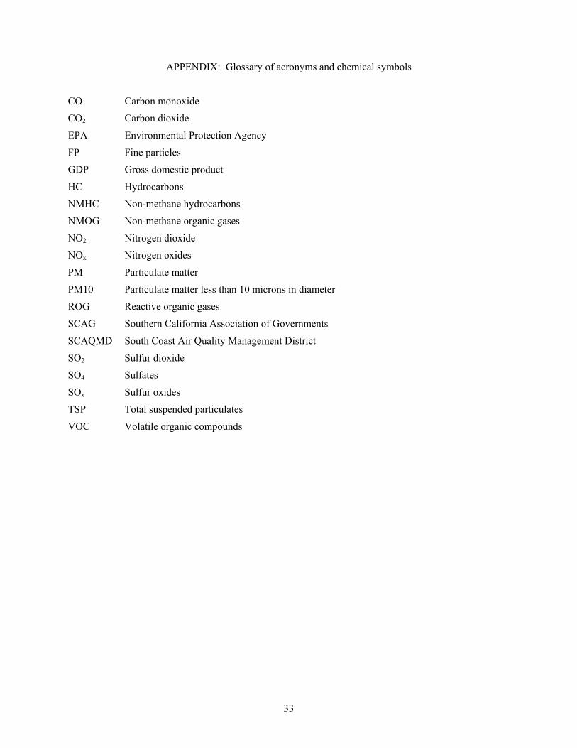
(NOx). (See the appendix for a glossary of acronyms and chemical formulae.) VOCs, also known as

2

reactive organic gases (ROG), give car exhaust its characteristic smell. VOCs react with NOx in the

atmosphere to form a variety of damaging oxidants such as ozone (O3), and they also produce secondary

carbon, a component of particulate matter (PM).

The main ingredient of VOCs is hydrocarbons (HC), which are emitted primarily as unburned

components of petroleum. Another ingredient is oxyhydrocarbon compounds, such as formaldehyde,

which are formed in the combustion process (National Research Council, 1991, p. 23). The lightest

hydrocarbon, methane, is less reactive than other components of VOC and is often excluded from

regulation; for these reasons, data are sometimes compiled as non-methane hydrocarbons (NMHC) or

non-methane organic gases (NMOG). For the most part we ignore these distinctions because the

quantitative differences among VOC, ROG, HC, NMOG, and NMHC are small for petroleum-based

motor vehicle emissions.

Motor vehicles, especially those using diesel fuel, emit some particulate matter directly and also

emit sulfur oxides (SOx), primarily sulfur dioxide (SO2). SO2 is an irritant and contributes to particulate

formation and acid rain. The same is true of nitrogen dioxide (NO2), which is formed in the atmosphere

from other NOx emissions and helps give smog its brown color. We do not explore the direct effects of

ambient SO2 and NO2 in this paper, but we do account for their role in particulate formation, which

appears to be more important to human health.

Table 1 shows the fractions for direct emissions of several pollutants that are estimated to come

from transportation activities. Figures such as these are sometimes summarized by the misleading

statement that half of all air pollution is from automobiles. Actually the fraction varies considerably by

pollutant and location, and tends to be much higher in urban areas as illustrated in the table by the figures

for Los Angeles.

In recent years, concern about motor vehicle emissions has broadened to include the global effects

of certain "greenhouse gases," mainly carbon dioxide (CO2), whose accumulation over decades or

centuries may cause a gradual warming of the earth's atmosphere (Cline, 1991). Such warming would be

accompanied by largely unknown but possibly dramatic changes in wind and rainfall patterns, and

possibly by rising sea levels. We return to the question of global warming at the end of the paper.

3

Emission Control Legislation

The primary legislation for controlling automobile emissions in the United States is the Clean Air

Act of 1963, amended in 1970, 1977 and 1990. The act provides a mechanism for setting ambient air

quality standards, which define the maximum acceptable concentrations of pollutants in the air. The

ambient standards apply to CO, O3, NO2, SO2, particulate matter of diameter less than 10 microns

(PM10), and lead. The act also specifies emission standards from motor vehicles, including tailpipe

emissions of CO, VOC, and NOx, and evaporative emissions of VOC. The state of California has even

stricter standards, mainly because its topography and climate tend to concentrate emitted pollutants and to

foster chemical reactions involving them.

Table 2 lists many of the past and future tailpipe standards for the United States and for California.

The new federal "tier I" and "tier II" standards, as well as the four newly specified vehicle classes for

California, are to be phased in starting in 1994. California has its own phase-in schedule, with the intent

of making motor vehicles account for only ten percent of ozone in the Los Angeles basin by the year

2010 (Calvert et al., 1993, p. 39).

In Europe, most countries prior to 1992 complied with emission standards set forth by the UN

Economic Commission for Europe. Exceptions include Austria, Denmark, Finland, Sweden, Norway,

and Switzerland, all of which have adopted somewhat stricter standards similar to those in the United

States. Beginning in 1992, nations in the European Community (now European Union) are required to

follow regulations promulgated by the Commission of the European Communities. Some of these

regulations are shown in Table 3. The standards are based on urban and "extra-urban" driving cycles

which differ from the U.S. federal test procedure. Overall the European restrictions are not as stringent as

in the United States: for example, the 1992 Euro I regulations for heavy-duty vehicles are similar to U.S.

standards in 1988, and the Euro II regulations effective 1995 are comparable to U.S. standards for 1991 (

).

On-Road Emissions

Actual on-road emissions are a different matter. Estimates and predictions of emissions in the U.S.

have mostly been made using either the federal MOBILE model or California's EMFAC model. These

4

models attempt to account for fleet composition, driving behavior, and aging of emission control devices.

However, three lines of evidence have recently cast doubt on the accuracy of these emissions

inventory models (Cadle et al., 1993; St. Denis et al., 1994). The first comes from measurements of

ambient concentrations in tunnels, where the volume of air and its rate of flow can be precisely measured.

Data from a tunnel under Van Nuys Airport near Los Angeles indicate that emissions of CO and NMHC

were 2.7 and 3.8 times higher than predicted by California's EMFAC model, version 7C (Ingalls, 1989;

Ingalls et al., 1989). Other tunnels show similar discrepancies with the U.S. federal MOBILE model

(Pierson et al., 1990). The second line of evidence is from airshed models that predict ambient

concentrations from an assumed spatial distribution of emissions. A comparison using version 7E of

EMFAC showed that ambient ratios of CO to NOx and of VOC to NOx were higher than could be

predicted, by factors of 1.5 for CO and 2-2.5 for NOx (Fugita et al., 1992). These discrepencies are

believed to represent under-estimation of CO and NMOG emissions. The third line of evidence is from

data collected to calibrate newly developed remote sensing devices that measure pollutants as they flow

out of tailpipes on moving vehicles (Lawson et al., 1990; Stephens and Cadle, 1991; Bishop et al., 1993).

At least two reasons have been offered as to why the models under-predict CO and VOC

emissions. First, they under-represent both the frequency and the severity of gross polluters. The remote

sensing experiments have shown that roughly 10 percent of the vehicles produce over 50 percent of CO

emissions, and there are strong indications that inspection programs are ineffective in maintaining

emission control systems (Glazer et al., 1995). Second, the models are based upon a federal test

prodedure that inadequately accounts for occasional hard accelerations (St. Denis et al., 1994).

As a result of this evidence, more recent versions of the models have been modified by raising the

assumed emissions rates from motor vehicles. The current version of EMFAC (EMFAC7F) has largely

eliminated the discrepancy for CO, but is still believed to under-predict VOC by a factor of approximately

2.1.1

Table 4 lists estimated average emission rates of CO, VOC, NOx, SOx, and PM10 for each of

1 Telephone conversation with Bart Croes, California Air Resources Board, Sacramento, August 1994.

See also Fujita and Lawson (1994), p. 1-4 and Table 3-11 for estimates of roughly the same magnitude.

5

sixteen vehicle types.2 These vehicle types include the fleet-average on-road emissions for gasoline

automobiles, light-duty diesel trucks, and heavy-duty diesel trucks for years 1992 and 2000.3 The figures

for CO are provided for completeness, but are not subsequently used in this paper. We have increased the

VOC estimates for gasoline automobiles by a factor of 2.1 to correct for the under-prediction problems

with EMFAC7F. (Later, we similarly increase the motor-vehicle portion of the total VOC inventory by

the same factor.) Other vehicle types shown in the table are recent model diesel cars and trucks, and new

cars meeting some of the new federal and California standards discussed earlier. These new car standards

are not adjusted for the VOC discrepancy or any type of deterioration. For comparison, we also show

emission rates for a composite of automobiles of various ages that met 1977 standards when new.

Throughout the table, diesel SOx emissions assume use of the low-sulfur diesel fuel now required in the

Los Angeles air basin.

3. Methodology of Damage Estimation

There are at least three ways to infer the costs of air emissions. The best developed, and the one

adopted here, is the direct estimation of damages. In this method, one traces the links between air

emissions and adverse consequences and attempts to place economic values on those consequences.

Examples include Small (1977), U.S. Federal Highway Administration (1982, p. E-47), Krupnik and

Portney (1991), and Hall et al. (1992). Other methods include hedonic price measurement, in which

2 For the sake of clarifying our calculations, we show figures in this and subsequent tables with more

significant digits than is justified by the precision of the estimates.

3 The fleet average consists of all types and ages of the appropriate vehicle category, weighted by vehicle-

miles traveled in the entire state of California as calculated by the EMFAC7F model. Total particulate

matter (PM) emissions are converted into PM10 based on the estimate that 99.4% of gasoline-powered

vehicle PM emissions and 96% of diesel-powered vehicle PM emissions are PM10 (telephone conversation

with Robert Effa, California Air Resources Board, Sacramento, May 1994).

6

observed price differentials are related to air quality; and revealed preference of policy makers, in which

pollution costs are inferred from the costs of meeting pollution regulations.

In the method of direct damage estimation, several links in the causal chain must be separately

measured (Hall et al., 1992). A pollutant emitted into the atmosphere changes the spatial and temporal

patterns of ambient concentrations of that pollutant and perhaps others. These patterns are determined by

atmospheric conditions, topographical features, and the presence of other natural or man-made chemicals

in the air. The resulting ambient concentrations then interact with people, buildings, plants, and animals

in a way that depends on their locations and activity levels. The results may be physical and/or

psychological effects: coughing, erosion of stone, retarded plant growth, injury to young, loss of

pleasurable views, and so forth. Finally, these effects have an economic value.

Most studies of direct damages find that human health effects are the dominant component of air

pollution costs. We therefore focus our efforts on the various causal links that lead to deterioration of

human health.

In any concrete application, there are several conceptual and practical issues to be resolved. We

discuss four in this section.

Willingness to Pay

Economists widely accept the principle that in market economies the social cost of a change in

economic outcomes is most usefully measured by the sum of individuals' willingness to pay for that

change, given their current economic circumstances. The underlying argument is that if public policy

consistently uses such valuations, most people will find that their overall welfare is improved (Hotelling,

1938; Hicks, 1941). Thus to measure the cost of increasing people's frequency of headaches, one tries to

determine how much they would be willing to pay to reduce that frequency, assuming they are presented

with full information and clear choices.

Similarly, the appropriate valuation of small increases in the risk of dying from lung disease is the

amount that people are willing to pay to marginally reduce that risk. It turns out that there many

situations in which one can observe such a quantity, particularly in the labor market where jobs with

varying risk levels command compensating wage differentials. Excellent reviews and conceptual

7

discussions include Kahn (1986), Fisher et al. (1989), Jones-Lee (1990), and Viscusi (1993). When

studies with clear biases are eliminated, the evidence consistently shows that people in nations with high

standards of living are willing to pay over one thousand dollars per year to reduce their annual mortality

risk by 1 in 1,000: that is, their average "value of life" is more than one million dollars. Fisher et al.

(1989) make an excellent case for a valuation between $2.1 million and $11.3 million at 1992 prices.4

We take this as the most reasonable range, and choose the geometric mean ($4.87 million) as our best

estimate. When price levels are adjusted for, this mean value is very close to the figure adopted by Hall et

al. (1992), and is about half the value recommended by Kahn (1986).5

Joint Costs and Nonlinear Effects

Nonlinear relationships may occur at several points in the chain of causality linking emissions to

costs: in the formation of ozone from VOC and NOx emissions, in the exposure of people to ambient

pollution concentration, and in the biological response to such exposure. This means that the cost of a

given emission depends on what pollutants are already in the air, and total costs cannot necessarily be

allocated among its constituents.

Ozone formation provides an especially difficult example (National Research Council, 1991).

Ozone in the lower atmosphere is created through complex chemical reactions involving volatile organic

compounds and nitrogen oxides. If the ratio of ambient levels of VOC to NOx is high, ozone formation is

said to by "NOx-limited," i.e., at the margin ozone depends just on NOx emissions. If the VOC/NOx ratio

4 We inflate by U.S. gross domestic product per capita, on the assumption that people's valuations grow

with income. GDP per capita grew 33.3 percent from 1986 to 1992, from U.S. Council of Economic

Advisors (1994), Table B-6.

5Krupnik and Portney (1991) argue that people place a lower value on risk of death from air pollution than

is inferred from labor market studies because deaths from air pollution occur on average to older people who

would have shorter life expectancies. Fisher et al. (1989), in contrast, point out that people demand greater

compensation for risks that are out of their control.

8

is low, ozone formation is "VOC-limited" so that reducing NOx has little marginal effect (and may even

increase ozone in the immediate vicinity of the sources). Recent evidence has led scientists to conclude

that VOC emissions from both natural and man-made sources are higher than previously believed; this

has raised estimates of VOC/NOx ratios, so there is a renewed interest in control of NOx (National

Research Council, 1991).

Most other relationships appear reasonably approximated by linear ones at the relatively low

chemical concentrations, measured in parts per million or parts per billion, with which we are concerned.

This is an important and essential simplification, so it is worth defending in some detail.

The ambient concentration of a primary (i.e., directly emitted) pollutant will be proportional to

emissions if it is removed from a given volume of air at a rate proportional to its concentration. This is

normally the case, and therefore a proportional linear relationship is widely used for primary pollutants

(Ball et al., 1991, p. 30). Even for secondary pollutants such as ozone, concentrations tend to be close to

linear functions of equiproportionate increases in precursor emissions over much of the range of interest.

For example, graphs relating predicted average ozone concentrations in the Los Angeles basin to

percentage regionwide cutbacks in VOC and NOx emissions show that ambient ozone declines very close

to linearly as its precursors are reduced by equal percentages (Milford et al., 1989, fig. 13).6 Secondary

pollutant formation appears more nonlinear if one measures it by extremes, such as the peak concentration

regardless of location in an air basin.7 Such a measure is appropriate for analyzing compliance with legal

air quality standards, but not for computing social costs throughout a region.

With respect to health effects, there are several reasons to accept linearity between concentrations

6 This can be seen by the nearly equal spacing between isopleths as one moves along a diagonal line

connecting the points representing no control and 100 percent control of both precursors. Note that our

argument for ozone is for linearily, not proportionality.

7 An example is Milford et al. (1989), fig. 11, reprinted in National Research Council (1991), p. 176.

Even this figure is very close to linear along a ray from baseline emissions down to about 50 percent

cutbacks in both precursors, and along several other rays as well.

9

and aggregate health costs as a good approximation for aggregate analysis. Numerous reviews of health

effects of various pollutants have found no convincing evidence of threshholds in most cases: for

example National Academies of Science and Engineering (1974, pp. 6, 190, 366-367, 400) and Schwartz

et al. (1988). Nonlinearities in dose-response relationships are sometimes assumed without evidence

because of the legal status of ambient air standards; yet these standards are determined more by the

sensitivity of the studies upon which they are based than by any evidence of thresholds (Horowitz, 1982,

pp. 113-115). Even when a threshold was thought to exist, further research has often uncovered evidence

of effects below that threshold, as described by Dockery et al. (1993) for particulates and Lippmann

(1993) for ozone. Finally, any nonlinearities that may exist for individuals or for specific locations will

be reduced or eliminated in aggregate populations by the effects of averaging over individual

susceptibilities, behavior patterns, and locations.

Exposure

While considerable scientific effort has gone into the atmospheric modeling necessary to predict

ambient air concentrations, far less has gone into understanding where and when people actually become

exposed to those concentrations. Yet concentrations vary widely over time and space, and people's

exposure depends heavily on whether they are indoors or outdoors, in or out of a vehicle, and how

strenuously they are exercising. Hall et al. (1992) pioneer the use of comprehensive models to quantify

this exposure, and some of our estimates make use of their results.

4. Estimates for the Los Angeles Region

In this section we estimate the per-mile costs of air emissions from various classes of motor

vehicles in the Los Angeles region. We do so within a framework that can be readily updated to reflect

new information or alternative assumptions. Unless otherwise stated, all monetary figures are in U.S.

dollars at 1992 prices.

Because the topography of Los Angeles tends to trap pollutants and the climate favors

photochemical reactions, the costs of a given amount of emission are likely to be higher than in most

10

areas. For example, Small (1977, pp. 123-124) assembles evidence that meteorological conditions

produce about six times as many days with low mixing heights and wind speeds in Los Angeles as in

other 12 U.S. cities outside California. In addition, our valuation of risk of death is applicable only to

developed nations.

Attempting to focus on the avenues of damage that current evidence suggests are most important,

we estimate three main categories of costs: mortality from particulates, morbidity from particulates, and

morbidity from ozone. We do not treat carbon monoxide despite its known adverse health effects and its

importance in pollution control strategies because there is little or no quantitative information suitable for

measuring its health costs (Hall et al., 1992). The only estimates available are extremely low and not

applicable to ground-level emissions (Davis and Chaudhry, 1993). Work in progress may remedy this

deficiency (Delucchi et al, forthcoming), but we believe it will show CO to be of less importance in

costing motor vehicle emissions than either particulates or ozone.

Mortality: Particulates

Evans et al. (1984) review the extensive statistical evidence linking mortality in U.S. metropolitan

areas to ambient pollution concentrations. They conclude:

We are of the opinion that the cross-sectional studies reflect a causal relationship between exposure to air-borne particles and premature mortality.... However, we are in the minority in taking this view. (p. 78)

They also conclude that "the apparent association is weak to moderate in strength, [and] that the specific

type of particle responsible has not been identified...." (p. 78)

Subsequent studies provide further support for their opinion that particulate matter causes

increased mortality. These studies also suggest that inhalable particles, i.e. particulate matter of diameter

less than 10 microns (PM10), are the most responsible. Among the components of PM10, the most

consistently found effects are from fine particles (FP), which are those with diameter less than 2.5

microns, and from sulfates (SO4), which are mainly aerosols of aluminum sulfate.8

8 Sulfate particles that are small enough in size are included in PM10 and FP.

11

Özkaynak and Thurston (1987) and Dockery et al. (1993) provide two of the most compelling such

studies. Özkaynak and Thurston use cross-sectional data from 1980, when pollution measurements were

much more complete and accurate than in earlier years. As in the studies reviewed by Evans et al. (1984),

they relate mortality in metropolitan areas to ambient pollutant concentrations in the downtown areas of

their central cities. They use four alternative measures of particulates: total suspended particulates (TSP),

PM10, FP, and SO4. The strongest and most consistent relationship is obtained using SO4, and the next

strongest using FP. The broader categories, PM10 and TSP, are not reliably correlated with mortality

when other control variables are taken into account. An effort to trace fine particulates to their source

type provides suggestive though inconclusive evidence that particulates arising from the metals and coal

industries are more damaging than those arising from automobiles, the oil industry, or windblown soil.

Dockery et al. (1993) describe the only study based on micro data to address these same issues.

They construct proportional hazard models to explain mortality among 8,111 adults in six U.S. cities,

each followed for up to 16 years. They find strong effects of lagged values of pollution as measured by

SO4, FP, or PM10. These effects are not greatly affected by controls for smoking, education,

occupational exposure, and other variables. The effects are so strong that adjusted mortality rates (i.e.,

rates after controlling for other factors) go up by 26 percent as particulate levels are raised from those in

the least polluted of the six cities to those of the most polluted. This magnitude seems implausibly large

to us, so it is not used in our quantitative estimates.

From the results reviewed here, it seems clear that sulfate aerosols cause increased mortality, and

that other components of PM10 may also. These findings are consistent with other evidence that finer

particles are more readily deposited on human and animal airways than coarser particles, and that acidic

aerosols are especially damaging (U.S. EPA, 1982; Lippmann and Lioy, 1985). (As a result of such

findings, the TSP ambient standard in the U.S. was replaced by a PM10 ambient standard during the

1980s.) These observations provide two alternative hypotheses for estimating the dose-response

relationship: one based on the coefficient of FP, the other based on that of SO4, when each is separately

included as the sole pollution-related independent variable explaining mortality. We choose the results of

Özkaynak and Thurston (1987), Table III, model M1. The relevant coefficients are measured as the

increased annual metropolitan-area deaths per 100,000 population for a unit increase in particulate

12

concentration in micrograms per cubic meter (µg/m3) as measured at a central monitoring station. The

coefficients (standard errors in parentheses) are 6.6 (1.5) for SO4 and 2.2 (0.8) for FP. If we assume that

all the constituents of PM10 (including FP) are equally harmful and that FP were a fixed proportion of

PM10 throughout the sample, then a coefficient for PM10 can be imputed. Lacking such data nationwide,

we use information for the Los Angeles region, where 59 percent of PM10 is FP (SCAQMD, 1994,

Appendix I-D); hence the imputed PM10 coefficient is 0.59x2.2 = 1.298.

An alternative and somewhat lower pair of coefficients is obtained by using the reanalysis by

Evans et al. (1984) of the 1960 data used by Lave and Seskin (1977). These estimates again show the

results of using one pollution measure at a time. The coefficients (standard errors in parentheses) are 3.72

(1.90) for SO4 and 0.338 (0.198) for TSP (Evans et al., 1984, Table 18). Based on the consensus that

PM10 rather than TSP causes health damages, we assume that among the constituents of TSP, only PM10

causes mortality; then the same coefficient (0.338) applies to changes in PM10.9

Another line of evidence comes from time series studies relating daily mortality rates to daily

concentrations of particulates. Schwartz (1994) performs a meta analysis of more than a dozen data sets,

finding that each increase in PM concentration of 1 µg/m3 increases total mortality by 0.06 percent.

Multiplying this by the current mortality rate in the Los Angeles region of about 870 deaths per 100,000

people (U.S. Department of Health and Human Services, 1993, p. 1), we obtain a coefficient of 0.522,

which lies between the higher and lower values just discussed. This is reassuring, although we believe

the time series evidence is less appropriate because one cannot separate the long-term causal effects of

interest from the short-term timing of the course of a fatal illness. For example, a single day of high

pollution might trigger the deaths of many people weakened by diseases unrelated to air pollution; or at

the other extreme, daily deaths might show no correlation with daily pollution levels even though chronic

illnesses are caused by long-term exposures.

9Alternatively, Hall et al. (1992) impute a higher coefficient to PM10 by implicitly assuming that all

components of TSP are equally harmful and that PM10 is serving as a proxy for all TSP, just as we assume

that FP is a proxy for all PM10.

13

PM10 concentrations result directly from emission of particulates and indirectly from emission of

VOC, NOx, and SOx. NOx and SOx react in the atmosphere, particularly in clouds, to form droplets of

nitric and sulfuric acid and also particles of ammonium nitrate and ammonium sulfate (Charlson and

Wigley, 1994). SCAQMD (1994, Appendix I-D) estimates that direct particulate emissions from motor

vehicles account for 10.6% of PM10, and that the indirect components from motor vehicle emissions are

as follows: 4.4% of PM10 is secondary carbon from VOC emissions, 10.5% is ammonium nitrate from

NOx, and 5.3% is ammonium sulfate from SOx.

Our calculations require estimates of ambient pollution levels and emissions, so that a given

reduction of emissions can be translated into a reduction in ambient levels. For the ambient PM10

concentration, which fluctuates from year to year due to weather, we average four years of annual-

average observations at the downtown Los Angeles monitoring site from 1987 through 1990 (Cohanim et

al., 1991, Tables 34-37). This gives a value of 57.8 µg/m3. We use the Los Angeles site because it is

most comparable to the downtown locations of the monitors used in the cross-sectional mortality studies

that underlie our mortality calculations. As an alternative scenario, we redo the calculation using the San

Bernardino monitoring site, whose annual average PM10 concentration of 77.75 µg/m3 is the highest in

the region.

For emissions, which are more stable, we use regionwide data for the year 1990.10 These data

include both natural (e.g. soil and marine salt) and human sources. For those scenarios in which all

components of PM10 are assumed to contribute equally to mortality, costs are allocated to precursor

emissions using source contribution percentages from SCAQMD (1994).11 We also compute a scenario

10 Originally estimated emissions in tons per day during 1990 were: VOC, 1,469; NOx, 1,290; SOx, 121;

and PM10, 838. Of these the following amounts were direct emissions from on-road vehicles: VOC, 761;

NOx, 762; SOx, 31; and PM10, 70. Source: SCAQMD (1994), Table 3-2A. Applying the correction factor

of 2.1 to on-road VOC emissions (see text) increases the VOC figures to 2,306 total and 1,598 on-road.

11For example, 10.5% of ambient PM10 at the downtown Los Angeles monitoring station is ammonium

nitrate traceable to on-road vehicle NOx emissions (calculated from SCAQMD, 1994, Appendix I-D, Table

14

in which only sulfates are assumed responsible for mortality, which as noted earlier is consistent with the

evidence; this is done by attributing all mortality to SOx emissions.12

The total PM10 inventory used as the basis for the above percentages includes geological sources

such as soil particles and road dust. We have not included road dust as a motor vehicle emission, partly

because its emissions inventory is thought to be especially unreliable and is currently under review.

Morbidity: Particulates and Ozone

Hall et al. (1992) report the results of an elaborate exposure model for the Los Angeles region in

which the spatial distributions of pollution and people's activity patterns are combined with estimated

hours of exposure under various locations (indoors, outdoors, and in-transit) and breathing rates (sleeping,

3-2). Therefore the 762 tons/day (278,130 tons/year) of on-road NOx emissions (see previous footnote) add

0.105x57.8 = 6.069 µg/m3 to the PM10 concentration. Applying Evan's mortality coefficient, for example,

these emissions are responsible for an increase in annual mortality of 0.338x6.069 = 2.0513 deaths per

100,000 people per year. In a region with 12 million people this means 2.0513x120 = 246 deaths caused by

278,130 tons of NOx emissions. Assuming a proportional rollback model and valuing deaths at our central

estimate of $4.87 million yields an estimate of cost of mortality of 246x($4.87 million)/278,130 =

$4,310/ton. Similar calculations were performed for VOC, SOx, and direct PM10 emissions.

12 The calculation is similar to the NOx example of the previous footnote except that ammonium sulfate is

the only component of PM10 that is assumed to contribute to mortality. An estimated 5.33% of ambient

PM10 at the downtown Los Angeles monitoring station is ammonium sulfate traceable to on-road SOx

emissions. Therefore the 31 tons/day (11,315 tons/year) of on-road SOx emissions add 0.0533x57.8 =

3.0807 µg/m3 to ambient sulfate concentrations. Applying the geometric average of Özkaynak-Thurston's

and Evan's sulfate coefficients, which is (6.6x3.72)1/2 = 4.955, these emissions are responsible for an increase

in annual mortality of 4.955x3.0807 = 15.265 deaths per 100,000 people. Given a population of 12 million,

this means 15.265x120 = 1,831.8 deaths from 11,315 tons of SOx emissions; valuing each statistical death at

$4.87 million yields a cost of $788,400/ton.

15

at rest, exercising). Dose-response functions for a variety of acute effects such as coughing and eye

irritation are applied to these exposures, and the resulting effects are valued according the results of

contingent valuation surveys. Certain details of their model have been criticized by Harrison and Nichols

(1989), who claim that Hall et al. overestimated the costs. As a result, Krupnick and Portney (1991)

apply their own less elaborate modeling scheme for the case of ozone effects, though not for particulates.

Krupnik and Portney also incorporate newer evidence on dose-response relationships, including many of

the studies recently reviewed by Ostro (1994).

Because we are unable to disentangle the many parts of these very detailed models, we use the

resulting costs reported by Hall et al. and by Krupnik and Portney as high and low estimates, respectively,

of morbidity costs. Their results appear to estimate the costs that would be saved if pollution levels in the

Los Angeles region were lowered according to the 1989 Air Quality Management Plan (SCAQMD and

SCAG, 1989). We estimate the precursor emissions with and without this plan and attribute the

morbidity costs to these precursors in accordance with simple models of how those precursors produce

ambient concentrations of PM10 and ozone.

Ozone is formed as a result of emissions of VOC and NOx. Suppose as an approximation that the

function f(EV,EN) relating them is homogeneous of degree one, so that doubling both types of emissions

would double ozone concentration. Then the total effect of the two types of emission is allocable to each

in amounts proportional to their marginal effects, fV�f/�EV and fN�f/�EN: that is, f(EV,EN) =

fVEV+fNEN. (This is an application of the Euler Theorem.) Equivalently, the elasticity of ozone

concentration with respect to VOC emissions, (EV/f)(�f/�EV), is the fraction EVfV/(EVfV+ENfN).

Empirical measurements of the function f indicate that in realistic situations it is entirely plausible

for this fraction to lie anywhere between zero (NOx-limited) and one (VOC-limited), or even to be greater

than one (when ozone declines as NOx increases). For example, Mayeres et al. (1993, fig. 6) present iso-

ozone curves for Belgium which imply that the ratio ranges from zero (under scenarios with 30 percent or

more NOx redution from present levels) to about 1.5 (under scenarios with 15 percent or more VOC

reduction from present levels). A similar range applies to the iso-ozone curves for several sites in the Los

Angeles region computed by Milford et al. (1989, figs. 4, 11). According to them, meeting U.S. federal

ozone standards would require very large reductions in both NOx and VOC, and ozone would then be

16

NOx-limited so that fV would be zero. (One reason for this is that there are substantial natural sources of

VOC.) Under current conditions, on the other hand, their graphs show modest NOx reductions to be

ineffective or even counter-productive in lowering ozone in the most heavily populated areas of the

region, so that fN is near zero or even negative. Between these extremes are many starting points for

which both VOC and NOx reductions are effective.

We therefore consider three alternative scenarios in which the elasticity of ozone with respect to

VOC emissions is zero, one, or one-half. This amounts to allocating the health benefits of ozone

reduction entirely to NOx, entirely to VOC, or equally to NOx and VOC.

For particulate morbidity, Hall et al. estimate an annual cost saving of $919 million in 1992

prices13 for meeting federal ambient air standards in the year 2010. The same estimate is used by

Krupnick and Portney. It is based on modeling done for the 1989 air quality management plan, which

shows a required reduction in PM10 concentrations, projected for the year 2010, of 48.3 µg/m3 (from

73.8 to 25.5) (SCAQMD and SCAG, 1989, Figure 5-7). This gives us a cost estimate of $19.03 million

per year for each one-unit change in PM10 concentration. We allocate this cost to the four primary

emissions in exactly the same way as for particulate mortality.14

For ozone morbidity, both Hall et al. (1992) and Krupnick and Portney (1991) estimate the annual

cost of failing to meet U.S. federal ozone standards. Their results, again in 1992 prices, are $3.2 billion

and $0.36 billion, respectively. Meeting those standards would require an 87.5% reduction in total VOC

emissions (including natural sources) and a 79.9% reduction in NOx emissions, or 1,275 and 813

13We have inflated their $775 million estimate, which was in 1988 prices, by the consumer price index,

consistent with their treatment of price levels. It makes virtually no difference if we instead inflate by GDP

per capita.

14Again using the ammonium nitrate portion of PM10 as an example, a 48.3 µg/m3 reduction in ambient

PM10 valued at $919 million leads to a value of NOx emissions of ($919,000,000/48.3 µg/m3) x (0.105 x

57.8 µg/m3)/(762x365 tons/year) = $415/ton.

17

tons/day, respectively.15 This enables us to allocate the health costs of morbidity to NOx, SOx, or a

combination of the two, as described earlier.16 Admittedly we are stretching the linearity assumptions by

applying them to such large reductions.

Results: Costs per Unit of Emission from Motor Vehicles

Our calculations of the cost per ton of emissions of various pollutants are shown in Table 5, for

alternative sets of assumptions. The table reveals that mortality from particulate matter is the dominant

component of costs of VOC, NOx, SOx, and PM10 emissions. For NOx, costs arising from the production

of secondary particulate matter are several times higher than those from the production of ozone, although

there are some combinations of assumptions for which this is not the case. For VOC, costs from

secondary particulate formation are about 50 percent higher than those from ozone production under

baseline assumptions. It appears likely, then, that particulate matter creates a more serious health problem

than ozone, even in Los Angeles with its notorious ozone concentrations.

Because mortality is the dominant cost, our cost estimates are sensitive to assumptions about

15The applicable air quality management plan shows emissions in a baseline scenario (1989 control

policies) for the year 2010, and reductions needed to meet the federal standards (SCAQMD, 1989, Tables 4-

1, 4-11, and 4-14). For VOC, baseline emissions are 1,130 tons/day; the reduction is 948 tons/day, of which

327 tons/day is from transportation sources. We assume that the transportation-related VOC reductions

required are underestimated by a factor of 2.0 (i.e, by 327 tons/day), and that total baseline VOC emissions

are underestimated by the same absolute amount (327 tons/day). Hence total baseline emissions of

1130+327=1457 tons/day would be reduced by 948+327=1275, or 87.5%. We use the factor 2.0 instead of

2.1, used elsewhere, because we apply it to all transportation sources instead of just gasoline-powered

vehicles.

16For example, using the higher ozone morbidity estimate of $3.2 billion from Hall et al., allocating the

cost equally to both types of emissions yields cost estimates for VOC of ($1.6 billion/year)/(1275x365

tons/year) = $3,438/ton, and for NOx of ($1.6 billion/year)/(813x365 tons/year) = $5,392/ton.

18

mortality coefficients and value of life. Using the lowest assumptions about both reduces our cost

estimates for SOx and PM10 by a factor of about 4.5; using the highest assumptions raises them by the

same factor. Cost estimates for VOC and NOx emissions are somewhat less sensitive. Cost estimates for

specific emissions are altered a great deal if particulate damage is assumed to be due only to sulfates.

Only the costs of VOCs, and to a lesser extent of NOx, are sensitive to how ozone damage is allocated.

Results: Costs of Motor Vehicle Emissions

Table 6 shows the results of applying these estimates of cost per ton to the emissions of a 1992

California fleet-average gasoline-powered automobile. (Those emissions were shown in Table 3.) Under

the baseline assumptions, total cost is just over 3 cents per vehicle-mile. Nearly half of this cost is from

NOx, due largely to its role in particulate formation. Close behind in damaging potential is VOC,

followed by SOx and finally directly emitted PM10.

Under various assumptions, costs range from 1.4 to nearly 12 cents per vehicle-mile. Surprisingly,

the cost goes up if we assume that mortality arises only from sulfates instead of all PM10; this result

would change if the sulfur content of gasoline were reduced. Whether ozone damage is allocated to VOC

or NOx makes little difference to these estimates.

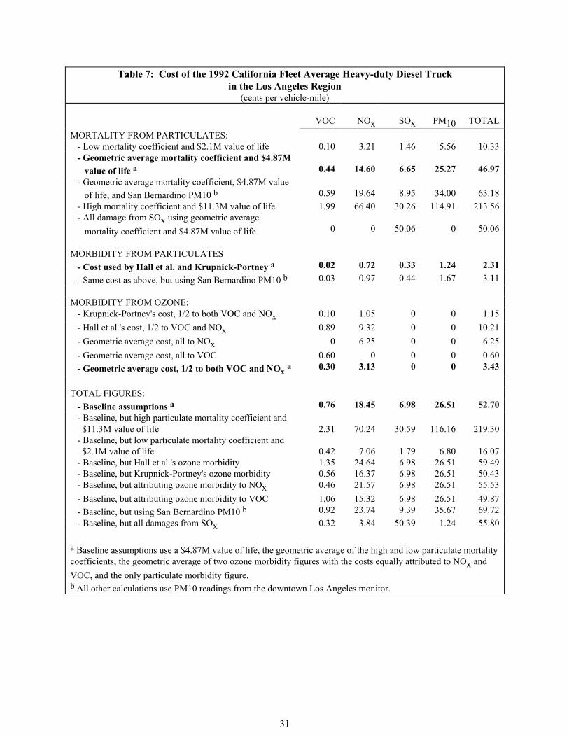
Table 7 shows a very different situation for a 1992 California fleet-average heavy-duty diesel truck

using the low-sulfur fuel required in Los Angeles. Its costs are very high: 53 cents per vehicle-mile

under baseline assumptions, with a range from 16 cents to $2.19. More than half the damage comes from

direct emissions of PM10, and another third from NOx. Total costs are slightly larger if all mortality is

assumed to be from sulfates.

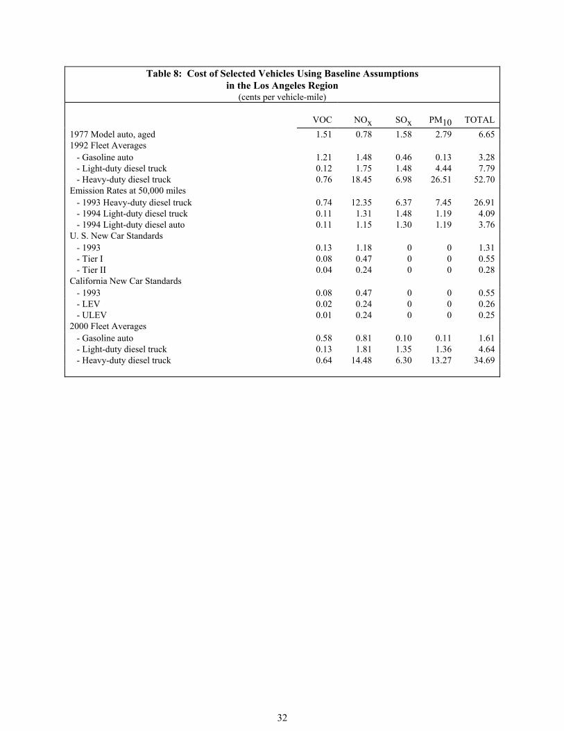
Table 8 shows our baseline cost estimates • that is, under intermediate assumptions • for each of

the vehicles whose emissions were previously presented in Table 3. Diesel cars, which differ little from

light-duty diesel trucks, are two to three times as costly as gasoline cars; this is mainly due to higher SOx

and PM10 emissions. New cars and trucks in 1993 are about half as costly as the 1992 fleet averages just

discussed. In the case of gasoline cars, the federal Tier I controls will reduce pollution cost from a new

vehicle by more than half compared to 1993 cars, to 0.6 cents per vehicle-mile. This remaining cost is

probably insignificant to vehicle use decisions, although it is equivalent to roughly half the total gasoline

19

taxes now paid by such a vehicle. These estimates for new cars are under the legally defined test cycle

and do not necessarily reflect on-road emissions.

Tighter standards will further reduce emissions from new trucks and buses after 1993; but slow

turnover produces a very high cost • 35 cents per mile • for the fleet average heavy-duty diesel truck in

the year 2000. This suggests that driving restrictions on heavy vehicles in urban areas may well be

justified, at least in areas like Los Angeles where the topography tends to concentrate pollutants.

As a sensitivity check, we recalculated these results under the assumptions that dust from paved

roads is attributable to motor vehicles and allocable on a per vehicle-mile basis. The result is to add about

4.3 cents/mile to the cost of all light-duty vehicles.17 As noted earlier, SCAQMD's inventory of road dust

is highly suspect so we do not give much credence to this estimate. Because paved road dust is not

reduced by current emissions control policies, is seems especially important to refine our knowledge

about this possibly large source of pollution costs.

Some Comparisons

How large is 3 cents per vehicle-mile, our baseline estimate for an average 1992 vehicle in

California? We can provide three useful points of comparison: earlier estimates of the same cost, likely

responses to internalizing the estimated costs, and estimates of other environmental costs of motor

vehicles.

An earlier estimate by Small (1977) of air pollution costs resulted in 0.61 cents/mile for a post-

1977 automobile operated in a California metropolitan area, stated in 1992 prices.18 This is only about

17Allocating SCAQMD's inventory of PM10 from paved road dust, which is 475.2 tons/day, among the

approximately 300 million daily vehicle-miles yields emissions of 1.23 g/mile.

However, the unit cost imputed to PM10 emitted as road dust is only about one-third that from other on-road motor-vehicle sources. The reason is that emitted quantities of PM10 in the SCAQMD inventory are about 6 times higher for road dust than for other motor-vehicle sources, whereas the fraction of ambient PM10 attributable to individual sources is only about twice as high; presumably this difference is because road dust settles out of the air more quickly than does other particulate matter from motor vehicles.

18 This inflates both health and materials costs by 3.466, the ratio of GDP per capital in 1992 to 1974 (U.S.

Council of Economic Advisers, 1994, Table B-6). California costs per unit of emissions, in $1000s per ton,

20

one-tenth of our estimate for the same vehicle shown in the top row of Table 8. The main reason for the

difference is that our baseline value of life is 29 times higher than the discounted lost earnings used by

Small (1977); that adjustment alone would bring the earlier estimate up to 5.34 cents/mile.19 The earlier

work also used different mortality estimates and a different method to allocate costs to specific emissions.

Next, consider what might happen if people were assessed charges or taxes of magnitude 3 cents

per vehicle-mile. At retail gasoline prices about $1.20 per gallon and fleet average fuel economy 23 miles

per gallon,20 this additional charge would be a bit more than half as large as current fuel cost per mile.

Past experience suggests that people pay attention to costs of such a magnitude, but not by altering their

amount of driving very much. For example, Greene (1992) estimates that raising the fuel cost per mile by

10 percent (either by raising fuel prices or by lowering fuel economy) reduces driving by 0.5-1.5 percent;

so if cars were charged a pollution tax equal to 50 percent of current fuel prices, people would drive just

2.5-7.5 percent fewer vehicle-miles. If the pollution tax varied with the vehicle's emission characteristics,

however, people would be given strong incentives to purchase cars with better pollution controls; so in

the long run the tax would decline and the effect on motor vehicle use would be even less, while adoption

of cleaner vehicles would be greatly facilitated.

In contrast to the case for automobiles, our baseline cost estimate of 53 cents per mile for the

average heavy-duty diesel truck is quite large. With fuel costs around 16 cents per mile and total

are: 0.06 for CO, 0.97 for VOC, 3.18 for NOx, 3.95 for SOx, and 1.87 for PM (at that time PM10 was not

distinguished either in data or regulations). These figures are computed as U.S. costs multiplied by 2.9 to

account for California topography and climate, as explained in Small (1977), pp. 123-124.

19Small (1977) included materials cost, and just under half of health costs were for premature deaths, so

raising value of life by a factor of 29 (4.87/0.166, to be exact) raises the final estimate only by a factor of 9.

The adjusted costs per unit emission in $1000s per ton are 0.88 for CO, 9.16 for VOC, 22.85 for NOx, 21.25

for SOx, and 26.45 for PM.

20The 1992 fleet average, from EMFAC7F input data.

21

operating expenses $1.30-$4.20 per mile,21 charging this pollution cost would cause a significant change

in trucking operations. Presumably, it would also greatly hasten the introduction of new lower-polluting

vehicles, thereby lowering the appropriate charges.

Finally, how much might global warming add to these cost estimates? The scientific basis for

estimating damage from global warming is especially shaky because its nature is so uncertain and its

anticipated effects, if they occur at all, will be cumulative and mostly far in the future. However, there is

considerable evidence from recent international agreements and negotiations about control measures that

may be adopted in the near term, and several analysts have estimated the costs of implementing them.

Manne and Richels (1992) estimate the lowest cost by which the United States could reduce emissions of

carbon dioxide along the following path: stabilization at 1990 levels up to the year 2000, then a gradual

20 percent reduction over the ensuing decade, followed by a maintenance of that reduced level

indefinitely. The marginal cost of emissions reduction eventually reaches about $208 per ton of carbon

(1990 prices), which is more than twice the size of a carbon tax proposed but never implemented in the

European Community. Updated to 1992 prices, this figure is equivalent to $0.67 per gallon of gasoline,

or 3.1 cents per vehicle-mile for an auto with U.S. average fuel economy.22

Such a cost would approximately double the pollution cost of the average automobile in Los

Angeles. Under the political scenarios underlying those hypothetical policies, global warming would

become the dominant air-pollution cost element as newer vehicles incorporating stricter pollution

standards are incorporated into fleets. It seems likely that a better assessment of future damage from

21The fuel cost assumes fuel price of $0.90 per gallon and fuel economy of 5.64 miles per gallon.

Operating expenses and intercity vehicle-miles for four classes of Class I intercity carriers are given in U.S.

Bureau of the Census (1993), Table 1047.

22Based on one ton carbon content for every 335 gal. refined petroleum product, calculated from Manne

and Richels (1992), p. 59; and 1991 average fuel consumption of 1 gal. per 21.7 miles, from U.S. Bureau of

the Census (1993), table 1037. Prices are deflated by the consumer price index for all items, from U.S.

Bureau of the Census (1993), table 756.

22

greenhouse gases will become increasingly important in determining the environmental damage from

motor vehicles.

5. Conclusion

Environmental policy frequently is forced into tradeoffs between cleaner air and economic

viability. We believe that the underlying basis for policy is clarified by making these tradeoffs explicit.

Accordingly we have estimated the air pollution costs from motor vehicles, focusing mainly on the Los

Angeles region. Our results probably give considerably higher estimates than would be obtained from

areas lacking the mountain barriers that trap pollutants in the Los Angeles air basin.

Our estimates measure the health costs from particulate matter and ozone. Although other costs

may be important, current evidence suggests that these constitute the bulk of the economic damage caused

by air pollution from motor vehicles in developed nations like the United States.

What these estimates suggest is that poorly controlled vehicles have significant pollution costs.

Costs are especially high for diesel cars and trucks, due to their high direct and indirect contributions to

ambient concentrations of particles. For most vehicles typical of the 1990s, however, air pollution costs

are not high enough so that internalizing them would alter automobile use very much. Our best estimate

for the cost of the average automobile on the road in Los Angeles in 1992 is $0.03, falling to half that

amount in the year 2000.

These findings make a strong prima facia case for policies that reduce the emissions from

individual vehicles. Changes to both vehicles and fuel can offer substantial aggregate cost savings. But

our findings do not provide much support for policies to reduce motor vehicle use overall. Such policies

might be justified on other grounds, but with good technological measures in place they cannot be

justified from the known costs of air pollution.

We do not address whether the particular pollution control policies now in place are good ones, a

question cogently discussed by Calvert et al. (1993). The kinds of cost estimates derived here can

contribute to the assessment of how stringent control policies should be.

Estimates of environmental costs are inherently uncertain. Among the many refinements that

23

would improve ours are measuring the health effects from carbon monoxide, nitrogen dioxide, and sulfur

dioxide; including damage to vegetation and building materials; and providing more sophisticated

modeling of the formation and transport of secondary pollutants. Probably the most important is

clarifying the role of road dust.

Nevertheless, we believe that estimates such as ours put the burden of proof on those who argue

that automobile use is greatly reducing the quality of life. It is not sufficient to simply point out that

motor vehicles are polluting; unless researchers can find quantitative links to economic loss that are

much stronger than those we have found, motor vehicle pollution seems best addressed by measures that

reduce the emissions associated with a given amount of motor vehicle use. Our estimates provide one

source of guidance as to which emissions it is most important to reduce.

24

Table 1: Proportion of Emissions Inventories Accounted for by Transportation Activities

Country CO VOCa NOx SOx

U.S.A. 66 48 43 N.A.

Los Angeles region 98 75b 83 68

Europe 78 50 60 4

U.K. 86 32 49 2

France 71 60 76 10

Germany 74 53 65 6

a Inventory for Europe is for hydrocarbons (HC). b Adjusted for assumption that motor vehicle emissions are 2.1 times those assumed in the

source (see text). Sources: Ball et. al (1991), Whitelegg (1993),

SCAQMD (1994).

25

Table 2: Exhaust Emission Standards for Gasoline-Powered Light-Duty Vehiclesa

(grams/mile)

Model Year U.S. Federal Standard California Standard

CO VOCb NOx CO VOCb NOx

Average pre-control car 84.0 10.6 4.1 84.0 10.6 4.1

1968-69 51.0 6.30 --c 51.0 6.30 --c

1970 34.0 4.10 -- 34.0 4.10 --

1971 34.0 4.10 -- 34.0 4.10 4.0

1972 28.0 3.00 -- 34.0 2.90 3.0

1973 28.0 3.00 3.0 34.0 2.90 3.0

1974 28.0 3.00 3.0 34.0 2.90 2.0

1975-76 15.0 1.50 3.1d 9.0 0.90 2.0

1977-79 15.0 1.50 2.0 9.0 0.41 1.5

1980 7.0 0.41 2.0 9.0 0.41e 1.0

1981-82 3.4 0.41 1.0 7.0 0.41e 0.7

1983-92 3.4 0.41 1.0 7.0 0.41e 0.4

1993 3.4 0.41 1.0 3.4 0.25f 0.4

Tier I (Calif.: TLEV) 3.4 0.25g 0.4 3.4 0.125f 0.4

Tier II (Calif.: LEV) 1.7 0.125g 0.2 3.4 0.075f 0.2

ULEV 1.7 0.040f 0.2

ZEV 0 0f 0

a Through 1993 the standard applies to new vehicles. Later standards apply at 5 years or 50,00 miles (10 years or 100,000 miles for federal tier II). Diesel vehicles must also meet standards for particulate matter starting in 1984 (California) or 1986 (U.S. federal).

b The standard is for hydrocarbons (HC), unless otherwise noted. c NOx emissions increased when left uncontrolled as HC and CO emissions were reduced. d New federal test procedure. e Optionally, can instead meet standard of 0.39 g/mi NMHC. f The standard is for NMHC. g The standard is for non-methane organic gases. Pollutants: California Vehicles: CO = Carbon monoxide TLEV = Transitional low emission vehicle VOC = Volatile organic compounds LEV = Low emission vehicle NOx = Nitrogen oxides ULEV = Ultra-low emission vehicle NMHC = Non-methane hydrocarbons ZEV = Zero emission vehicle Sources: Calvert, et al (1993, Tables 1-2); California Air Resources Board (1986; 1994, Table 2.).

26

Table 3: European Emissions Standards

Effective year

CO HC NOx Particulates Evaporative HC

Passenger Vehicles (g/km)

- 91/441/EECa 1992 2.72 0.97b 0.14 2.0 g/test

- 94/12/EC (proposed)

- gasoline powered 1997 2.2 0.5b N.A. N.A.

- diesel powered 1997 1.0 0.7b 0.08 N.A.

Heavy-Duty Diesels (g/kwh)

- Euro I 1992 4.5 1.1 8.0 0.36c N.A.

- Euro II 1995 4.0 1.1 7.0 0.15 N.A.

- Euro III (proposed) 1999 2.5 0.7 < 0.5

< 0.12 N.A.

a Standard shown is for "type approval." Applies to both gasoline and diesel cars. b A single standard applies to the sum of HC and NOx emissions. c For engines smaller than 85 kW, particulate emissions may be 1.7 times higher, or 0.612 g/kwh. N.A.: not available Source: CONCAWE (1992); and Inge Mayeres, personal communication, June 1994.

27

Table 4: Emission Factors for Selected Vehicles (grams per mile)

CO VOC NOx SOx PM10

1977 Model auto, aged a,b 3.900 4.700 0.660 0.130 0.248 1992 Fleet Averages c - Gasoline auto b 13.000 3.757 1.260 0.038 0.011 - Light-duty diesel truck d 1.607 0.362 1.492 0.122 0.395 - Heavy-duty diesel truck d 9.326 2.356 15.683 0.576 2.359 Emission Rates at 50,000 miles e - 1993 Heavy-duty diesel truck d 11.620 2.290 10.500 0.526 0.662 - 1994 Light-duty diesel truck d 1.220 0.351 1.110 0.122 0.106 - 1994 Light-duty diesel auto d 1.120 0.351 0.980 0.107 0.106 U. S. New Car Standards f - 1993 3.400 0.410 1.000 0 0 - Tier I 3.400 0.250 0.400 0 0 - Tier II 1.700 0.125 0.200 0 0 California New Car Standards f - 1993 3.400 0.250 0.400 0 0 - LEV 3.400 0.075 0.200 0 0 - ULEV 1.700 0.040 0.200 0 0 2000 Fleet Averages b,c - Gasoline auto 5.946 1.804 0.688 0.008 0.010 - Light-duty diesel truck 1.825 0.401 1.535 0.111 0.121 - Heavy-duty diesel truck 8.815 1.978 12.307 0.520 1.181 a From Small (1977), Table 5, row 9. PM10 is assumed to be 99.4% of PM (see footnote 2). b VOC emissions for gasoline automobiles are adjusted by a factor of 2.1 to reflect under estimation (see text). c EMFAC7F estimates from the California Air Resources Board. d The assumed SOx emissions from diesels in the EMFAC model overstate those for the Los Angeles region in the early 1990 because the sulfur content of fuel is lower in the region than elsewhere in California. We recalculated the emissions by assuming 0.05% elemental sulfur (S) content by weight, the legal standard in the region. We assume that fuel density is 3,249 grams/gallon and that each gram of S generates 2 grams of SO2: then SOx emissions = 0.0005 x 6498 = 3.249 grams/gallon of fuel. The 1992 fleet average light-duty and heavy-duty diesel trucks have fuel economy of 26.62 and 5.64 mpg from EMFAC. We assume that 1993 and 1994 diesel vehicles have the same fuel economy as the projected year 2000 fleet averages for the same vehicle types (e.g. 6.18 mpg for heavy-duty trucks and 26.5 mpg for light-duty trucks). For the year 2000 fleet averages, the EMFAC model is accurate for Los Angeles because by then most of the state will have the same sulfur standard for fuel content as Los Angeles currently has. e Air Resources Board's exhaust emission rates which are used as input to the EMFAC7F model. f From Table 2.

28

Table 5: Costs for the Los Angeles Region (1992 1000's $ per ton of emission)

VOC NOx SOx PM10 MORTALITY FROM PARTICULATES: $2.1M value of life - Low mortality coefficient 0.37 1.86 23.1 21.4 - Geometric average mortality coefficient 0.73 3.64 45.2 41.9 $4.87M value of life - Low mortality coefficient 0.86 4.31c 53.5 49.6 - High mortality coefficient 3.31 16.55 205.4 190.5 - Geometric average mortality coefficient a 1.69 8.45 104.8 97.2 - Geometric average mortality coefficient using San Bernardino PM10 b

2.27

11.36

141.0

130.7

$11.3M value of life - High mortality coefficient 7.67 38.41 476.5 442.0 - Geometric average mortality coefficient 3.92 19.60 243.2 225.5 All damage from SOx, $4.87M value of life - Geometric average mortality coefficient 0 0 788.4d 0.0 MORBIDITY FROM PARTICULATES - Cost used by Hall et al. and Krupnick-Portney a 0.08 0.42e 5.2 4.8 - Same cost as above, but using San Bernardino PM10 b 0.11 0.56 6.9 6.4 MORBIDITY FROM OZONE: Krupnick-Portney's cost figure - Attributing 1/2 to NOx, 1/2 to VOC 0.39 0.61 0 0 Hall et al.'s cost figure - Attributing 1/2 to NOx, 1/2 to VOC 3.44f 5.39f 0 0 Geometric average of Krupnick-Portney and Hall et al. - Attributing all damage to NOx 0 3.62 0 0 - Attributing all damage to VOC 2.31 0 0 0 - Attributing 1/2 to NOx, 1/2 to VOC a 1.15 1.81 0 0

TOTAL FIGURES: - Baseline Assumptions a 2.92 10.67 109.9 102.0 - Baseline, but attributing ozone morbidity to NOx 1.77 12.48 109.9 102.0 - Baseline, but attributing ozone morbidity to VOC 4.08 8.86 109.9 102.0 - Baseline, but attributing particulate mortality to SOx 1.24 2.22 793.6 4.8

- Baseline, but using San Bernardino PM10 b 3.53 13.73 147.9 137.1 a Baseline assumptions use a $4.87M value of life, the geometric average of the high and low particulate mortality coefficients, the geometric average of two ozone morbidity figures with the costs equally attributed to NOx and VOC, and the only particulate morbidity figure. b All other calculations use PM10 readings from the downtown Los Angeles monitor. c For the derivation of this estimate, see footnote 11. d For the derivation of this estimate, see footnote 12. e For the derivation of this estimate, see footnote 14. f For the derivation of this estimate, see footnote 16

29

30

Table 6: Cost of the 1992 California Fleet Average Gasoline Automobile in the Los Angeles Region

(cents per vehicle-mile) VOC NOx SOx PM10 TOTAL MORTALITY FROM PARTICULATES: - Low mortality coefficient and $2.1M value of life 0.15 0.26 0.10 0.03 0.54 - Geometric average mortality coefficient and $4.87M value of life a

0.70

1.17

0.44

0.12 2.43

- Geometric average mortality coefficient, $4.87M value of life, and San Bernardino PM10 b

0.94

1.58

0.59

0.16

3.27

- High mortality coefficient and $11.3M value of life 3.18 5.33 2.00 0.55 11.06 - All damage from SOx using geometric average mortality coefficient and $4.87M value of life

0

0

3.30

0

3.30

MORBIDITY FROM PARTICULATES - Cost used by Hall et al. and Krupnick-Portney a 0.03 0.06 0.02 0.01 0.12 - Same cost as above, but using San Bernardino PM10 b 0.07 0.08 0.03 0.01 0.16 MORBIDITY FROM OZONE: - Krupnick-Portney's cost, 1/2 to both VOC and NOx 0.16 0.08 0 0 0.24 - Hall et al.'s cost, 1/2 to VOC and NOx 1.42 0.75 0 0 2.17 - Geometric average cost, all to NOx 0 0.50 0 0 0.50 - Geometric average cost, all to VOC 0.96 0 0 0 0.96 - Geometric average cost, 1/2 to both VOC and NOx a 0.48 0.25 0 0 0.73

TOTAL FIGURES: - Baseline assumptions a 1.21 1.48 0.46 0.13 3.28 - Baseline, but high particulate mortality coefficient and $11.3M value of life

3.69

5.64

2.02

0.56

11.91

- Baseline, but low particulate mortality coefficient and $2.1M value of life

0.67

0.57

0.12

0.03

1.38

- Baseline, but Hall et al.'s ozone morbidity 2.16 1.98 0.46 0.13 4.72 - Baseline, but Krupnick-Portney's ozone morbidity 0.89 1.32 0.46 0.13 2.80 - Baseline, but attributing ozone morbidity to NOx 0.73 1.73 0.46 0.13 3.05 - Baseline, but attributing ozone morbidity to VOC 1.69 1.23 0.46 0.13 3.51 - Baseline, but using San Bernardino PM10 b 1.49 1.91 0.62 0.17 4.16 - Baseline, but all damages from SOx 0.51 0.31 3.32 0.01 4.15 a Baseline assumptions use a $4.87M value of life, the geometric average of the high and low particulate mortality coefficients, the geometric average of two ozone morbidity figures with the costs equally attributed to NOx and VOC, and the only particulate morbidity figure. b All other calculations use PM10 readings from the downtown Los Angeles monitor.

31

Table 7: Cost of the 1992 California Fleet Average Heavy-duty Diesel Truck in the Los Angeles Region

(cents per vehicle-mile) VOC NOx SOx PM10 TOTAL MORTALITY FROM PARTICULATES: - Low mortality coefficient and $2.1M value of life 0.10 3.21 1.46 5.56 10.33 - Geometric average mortality coefficient and $4.87M value of life a

0.44

14.60

6.65

25.27 46.97

- Geometric average mortality coefficient, $4.87M value of life, and San Bernardino PM10 b

0.59

19.64

8.95

34.00

63.18

- High mortality coefficient and $11.3M value of life 1.99 66.40 30.26 114.91 213.56 - All damage from SOx using geometric average mortality coefficient and $4.87M value of life

0

0

50.06

0

50.06

MORBIDITY FROM PARTICULATES - Cost used by Hall et al. and Krupnick-Portney a 0.02 0.72 0.33 1.24 2.31 - Same cost as above, but using San Bernardino PM10 b 0.03 0.97 0.44 1.67 3.11 MORBIDITY FROM OZONE: - Krupnick-Portney's cost, 1/2 to both VOC and NOx 0.10 1.05 0 0 1.15 - Hall et al.'s cost, 1/2 to VOC and NOx 0.89 9.32 0 0 10.21 - Geometric average cost, all to NOx 0 6.25 0 0 6.25 - Geometric average cost, all to VOC 0.60 0 0 0 0.60 - Geometric average cost, 1/2 to both VOC and NOx a 0.30 3.13 0 0 3.43

TOTAL FIGURES: - Baseline assumptions a 0.76 18.45 6.98 26.51 52.70 - Baseline, but high particulate mortality coefficient and $11.3M value of life

2.31

70.24

30.59

116.16

219.30

- Baseline, but low particulate mortality coefficient and $2.1M value of life

0.42

7.06

1.79

6.80

16.07

- Baseline, but Hall et al.'s ozone morbidity 1.35 24.64 6.98 26.51 59.49 - Baseline, but Krupnick-Portney's ozone morbidity 0.56 16.37 6.98 26.51 50.43 - Baseline, but attributing ozone morbidity to NOx 0.46 21.57 6.98 26.51 55.53 - Baseline, but attributing ozone morbidity to VOC 1.06 15.32 6.98 26.51 49.87 - Baseline, but using San Bernardino PM10 b 0.92 23.74 9.39 35.67 69.72 - Baseline, but all damages from SOx 0.32 3.84 50.39 1.24 55.80 a Baseline assumptions use a $4.87M value of life, the geometric average of the high and low particulate mortality coefficients, the geometric average of two ozone morbidity figures with the costs equally attributed to NOx and VOC, and the only particulate morbidity figure. b All other calculations use PM10 readings from the downtown Los Angeles monitor.

32

Table 8: Cost of Selected Vehicles Using Baseline Assumptions in the Los Angeles Region

(cents per vehicle-mile) VOC NOx SOx PM10 TOTAL 1977 Model auto, aged 1.51 0.78 1.58 2.79 6.65 1992 Fleet Averages - Gasoline auto 1.21 1.48 0.46 0.13 3.28 - Light-duty diesel truck 0.12 1.75 1.48 4.44 7.79 - Heavy-duty diesel truck 0.76 18.45 6.98 26.51 52.70Emission Rates at 50,000 miles - 1993 Heavy-duty diesel truck 0.74 12.35 6.37 7.45 26.91 - 1994 Light-duty diesel truck 0.11 1.31 1.48 1.19 4.09 - 1994 Light-duty diesel auto 0.11 1.15 1.30 1.19 3.76U. S. New Car Standards - 1993 0.13 1.18 0 0 1.31 - Tier I 0.08 0.47 0 0 0.55 - Tier II 0.04 0.24 0 0 0.28California New Car Standards - 1993 0.08 0.47 0 0 0.55 - LEV 0.02 0.24 0 0 0.26 - ULEV 0.01 0.24 0 0 0.252000 Fleet Averages - Gasoline auto 0.58 0.81 0.10 0.11 1.61 - Light-duty diesel truck 0.13 1.81 1.35 1.36 4.64 - Heavy-duty diesel truck 0.64 14.48 6.30 13.27 34.69

33

APPENDIX: Glossary of acronyms and chemical symbols

CO Carbon monoxide

CO2 Carbon dioxide

EPA Environmental Protection Agency

FP Fine particles

GDP Gross domestic product

HC Hydrocarbons

NMHC Non-methane hydrocarbons

NMOG Non-methane organic gases

NO2 Nitrogen dioxide

NOx Nitrogen oxides

PM Particulate matter

PM10 Particulate matter less than 10 microns in diameter

ROG Reactive organic gases

SCAG Southern California Association of Governments

SCAQMD South Coast Air Quality Management District

SO2 Sulfur dioxide

SO4 Sulfates

SOx Sulfur oxides

TSP Total suspended particulates

VOC Volatile organic compounds

34

References Ball, D.J., R.S. Hamilton, and R.M. Harrison (1991): "The Influence of Highway-related Pollutants on

Environmental Quality," in R.S. Hamilton and R.M. Harrison, eds., Highway Pollution, Elsevier, Amsterdam, pp. 1-47.

Bishop, G. A., D. H. Stedman, J. E. Peterson, T. J. Hosick, and P. L. Guenther (1993): "A Cost-

Effectiveness Study of Carbon Monoxide Emissions Reduction Utilizing Remote Sensing", Journal of Air and Waste Management, vol. 43, pp. 978-988.

Cadle, S.H., R.A. Gorse, and D.R. Lawson (1993): "Real-World Vehicle Emissions: A Summary of the

Third Annual CRC-APRAC On-Road Vehicle Emissions Workshop". Air and Waste, vol. 43, pp. 1084-1099.

California Air Resources Board (CARB) (1986): California New Vehicle Standards Summary: Passenger

Cars, CARB, Sacramento, June. California Air Resources Board (CARB) (1994): "Zero-Emission Vehicle Update: Draft Technical

Document for the Low-Emission Vehicle and Zero-Emission Vehicle Workshop". CARB, Sacramento, March.

Calvert, J.G., J.B. Heywood, R.F. Sawyer and J.H. Seinfeld (1993): "Achieving acceptable air quality:

Some reflections on controlling vehicle emissions". Science, vol. 261, 2 July, pp. 37-45. Charlson, R.J. and T.M.L. Wigley (1994): "Sulfate Aerosol and Climatic Change". Scientific American,

vol. 270 (February), pp. 48-57. Cline, W.R. (1991): "Scientific basis for the greenhouse effect". Economic Journal, vol. 101, pp. 904-

919. Cline, W.R. (1992): Global Warming: The Economic Stakes. Institute for International Economics,

Washington. Cohanim, S., M. Hoggan, R. Sin, L.W. Jones, M. Hsu, and S. Tom (1991): Air Quality Trends in

California's South Coast and Southeast Desert Air Basin (1976-1990), South Coast Air Quality Management District, Diamond Bar, California, August.

CONCAWE (1992): "Motor Vehicle Emission Regulations and Fuel Specifications - 1992 Update",

Report No. 2/92, Brussels, Belgium. Davis, C. and S. Chaudhry (1993): "Transportation Air Emission Cost Analysis". Appendix E of

California Energy Commission (CEC), Transportation Policy Impacts Hearing: 1993 California Transportation Energy Analysis Report, CEC, Sacramento, October.

35

Delucchi, M.A., D. McCubbin, J. Kim, J. Murphy, and S. Hsu (forthcoming): "The Annualized Social

Cost of Motor-Vehicle Use, Based on 1990-1991 Data". Draft report, Institute of Transportation Studies, University of California, Davis.

Dockery, D.W., C.A. Pope, X. Xu, J.D. Spengler, J.H. Ware, M.E. Fay, B.G. Ferris, Jr., and F.E. Speizer

(1993): "An Association between Air Pollution and Mortality in Six U.S. Cities". New England Journal of Medicine, vol. 329 (December 9), pp. 1753-1808.

Evans, J.S., T. Tosteson, and P.L. Kinney (1984): "Cross-Sectional Mortality Studies and Air Pollution

Risk Assessment". Environment International, vol. 10, pp. 55-83. Fisher, A., L.G. Chestnut, and D.M. Violette (1989), "The Value of Reducing Risks of Death: A Note on

New Evidence". Journal of Policy Analysis and Management, vol. 8, no. 1, pp. 88-100. Fujita, E.M., and D.R. Lawson (1994): "Evaluation of the Emissions Inventory in the South Coast Air

Basin". Desert Research Institute, Reno, Nevada, August. Fujita, E. M., B. E. Croes, C. L. Bennett, D. R. Lawson, F. W. Lurmann, and H. H. Main (1992):

"Comparison of Emission Inventory and Ambient Concentration Ratios of CO, NMOG, and NOx in California's South Coast Air Basin", Journal of Air and Waste Management, Vvl. 42, pp. 264-276.

Glazer, A., D. Klein, and C. Lave (1995): "Clean for a Day: Troubles with Smog Check". Journal of

Transport Economics and Policy, vol. 29, this issue. Greene, D.L. (1992): "Vehicle Use and Fuel Economy: How Big is the 'Rebound' Effect?" Energy

Journal, vol. 13, no. 1, pp. 117-143. Hall, J.V., A.M. Winer, M.T. Kleinman, F.W. Lurmann, V.Brajer, and S.D. Colome (1992): "Valuing the

health benefits of clean air". Science, vol. 255, 14 February, pp. 812-817. Harrison, D., Jr., and A.L. Nichols (1989): "Preliminary Comments on 'Economic Assessment of the

Health Benefits from Improvements in Air Quality in the South Coast Air Basin'". National Economic Research Associates, Cambridge, Massachusetts, August.

Hicks, J.R. (1941): "The Rehabilitation of Consumers' Surplus". Review of Economic Studies, vol. 8,

February, pp. 108-116. Horowitz, J.L. (1982): Air Quality Analysis for Urban Transportation Planning. MIT Press, Cambridge,

Massachusetts. Hotelling, H. (1938): "The General Welfare in Relation to Problems of Taxation and of Railway and

Utility Rates". Econometrica, vol. 6, pp. 242-269.

36

Ingalls, M. N. (1989): "On-Road Vehicle Emission Factors and Measurements in a Los Angeles Area

Tunnel", Paper No. 89-137.3, Air and Waste Management Association 82nd Annual Meeting, Anaheim, CA.

Ingalls, M. N., L. R. Smith, and R. E. Kirksey (1989): "Measurements of On-Road Vehicle Emission

Factors in the California South Coast Air Basin - Volume I: Regulated Emissions", Report No. SwRI-1604, Southwest Regional Instititute for the Coordinating Research Council, Atlanta, GA.

Jones-Lee, M. (1990): "The Value of Transport Safety". Oxford Review of Economic Policy, vol. 6, pp.

39-60. Kahn, S.(1986): "Economic Estimates of the Value of Life". IEEE Technology and Society Magazine,

vol. 5, June, pp. 24-31. Krupnick, A.J.. and P.R. Portney (1991): "Controlling urban air pollution: A benefit-cost assessment".

Science, vol. 252, 26 April, pp. 522-528. Lave, L.B., and E.P. Seskin (1977): Air Pollution and Human Health. Johns Hopkins University Press,

Baltimore. Lawson, D. R., P. J. Groblicki, D. H. Stedman, G. A. Bishop, and P. L. Guenther (1990): "Emissions from

In-use Motor Vehicles in Los Angeles: A Pilot Study of Remote Sensing and the Inspection and Maintenance Program", Journal of Air and Waste Management, vol. 40, pp. 1096-1105.

Lippmann, M. (1993): "Health Effects of Tropospheric Ozone: Review of Recent Research Findings and

their Implications to Ambient Air Quality Standards". Journal of Exposure Analysis and Environmental Epidemiology, vol. 3, no. 1, pp. 103-129.

Lippmann, M., and P.J. Lioy (1985): "Critical Issues in Air Pollution Epidemiology". Environmental

Health Perspectives, vol. 62, pp. 243-258. Manne, A.S. and R.G. Richels (1992): "Buying Greenhouse Insurance: The Economic Costs of Carbon

Dioxide Emission Limits". MIT Press, Cambridge, Massachusetts. Mayeres, I. (1992): "The Social Costs of Road Transport". Working paper, Centre for Economic Studies,

Katholieke Universiteit Leuven, Belgium, June. Mayeres, I., S. Proost, and D. Miltz (1993): "The Geneva Hydrocarbon Protocol: Economic Insights

from a Belgian Perspective". Environmental and Resource Economics, vol. 3, pp. 107-127. Milford, J.B., A.G. Russell, and G.J. McRae (1989): "A New Approach to Photochemical Pollution

Control: Implications of Spatial Patterns in Pollutant Responses to Reductions in Nitrogen Oxides and

37

Reactive Organic Gas Emissions". Environmental Science and Technology, vol. 23, October, pp. 1290-1301.

National Academy of Science and National Academy of Engineering (1974): Air Quality and Automobile

Emission Control. U.S. Government Printing Office, Washington. National Research Council (1991): Rethinking the Ozone Problem in Urban and Regional Air Pollution.

National Academy Press, Washington. Ostro, B. (1944): "Estimating the Health Effects of Air Pollution: A Method with an Application to

Jakarta", Policy Research Working Paper 1301, The World Bank, May. Özkaynak, H., and G.D. Thurston (1987): "Associations Between 1980 U.S. Mortality Rates and

Alternative Measures of Airborne Particle Concentration". Risk Analysis, vol. 7, no. 4, pp. 449-461. Pierson, W.R., A.W. Gertler, and R.L. Bradow (1990): "Comparison of the SCAQS Tunnel Study with

Other On-Road Vehicle Emission Data". Journal of the Air and Waste Management Association, vol. 40, pp. 1495-1504.

Quinet, E. (1993): "The Social Costs of Transport: Evaluation and Links with Internalisation Policies".

Joint OECD/ECMT Seminar on Internalising the Social Costs of Transport, 30 September - 1 October. Organisation for Economic Co-operation and Development, Paris.

Schwartz, J. (1994): "Air Pollution and Daily Mortality: A Review and Meta Analysis". Environmental

Research, vol. 64, pp. 36-52. Schwartz, J., V. Hasselblad, and H. Pitcher (1988): "Air Pollution and Morbidity: A Further Analysis of

the Los Angeles Student Nurses Data". Journal of the American Pollution Control Association, vol. 38, February, pp. 158-162.

Small, K.A. (1977): "Estimating the Air Pollution Costs of Transport Modes". Journal of Transport

Economics and Policy, vol. 11, May, pp. 109-132. South Coast Air Quality Management District (SCAQMD) and Southern California Association of

Governments (SCAG) (1989): Air Quality Management Plan: South Coast Air Basin. SCAQMD, El Monte, California, March.

South Coast Air Quality Management District (SCAQMD) and Southern California Association of

Governments (SCAG) (1994): Air Quality Management Plan: Meeting the Clean Air Challenge. SCAQMD, Diamond Bar, California, August.

St. Denis, M. J., P. Cicero-Fernández, A. M. Winer, J. W. Butler, and G. Jesion (1994): "Effects of In-Use

Driving Conditions and Vehicle/Engine Operating Parameters on 'Off-Cycle' Events: Comparison with

38

the Federal Test Procedure Conditions", Journal of Air and Waste Management, vol. 44, pp. 31-38. Stephens, R. D. and S. H. Cadle (1992): "Remote Sensing Measurements of Carbon Monoxide Emissions

from On-Road Vehicles", Journal of Air and Waste Management, vol. 41, pp. 39-46. U.S. Bureau of the Census (1993): Statistical Abstract of the United States. U.S. Government Printing

Office, Washington. U.S. Council of Economic Advisers (1994): Annual Report. With U.S. President, Economic Report of

the President. U.S. Government Printing Office, Washington. U.S. Department of Health and Human Services (1993): Monthly Vital Statistics Report: Births,

Marriages, Divorces, and Deaths, vol. 42, no. 6. U.S. Environmental Protection Agency (EPA) (1982): Air Quality Criteria for Particulate Matter and

Sulfur Oxides, vol. 3. EPA, Research Triangle Park, North Carolina. U.S. Federal Highway Administration (1982): Final Report on the Federal Highway Cost Allocation

Study. U.S. Government Printing Office, Washington. Viscusi, V.K. (1993): "The Value of Risks to Life and Health". Journal of Economic Literature, vol. 31,

no. 4, pp. 1912-1946. Whitelegg, J. (1993): Transport for a Sustainable Future: The Case for Europe. Belhaven Press, London.