0

Does Remedial Education at Late Childhood Pay Off After All? Long-Run Consequences for

University Schooling, Labor Market Outcomes and Inter-Generational Mobility*

Victor Lavy

University of Warwick

Hebrew University and NBER

Assaf Kott

Brown University

Genia Rachkovski

Northwestern University

Forthcoming Journal of Labor Economics

Abstract

We analyze the long-term effects of a high school remedial education program almost two decades after its

implementation. Treated students experienced an 11% increase in completed years of post-secondary schooling, a 4%

increase in annual earnings, and a significant increase in intergenerational income mobility. These gains mainly reflect

improvement of students from below median income families. We conclude that the program had gains beyond the

short term significant improvements in high-school matriculation exams. A cost benefit analysis of the program

suggests that the government will recover its cost within 7-8 years, implying a very high rate of return.

* Special thanks go to the Social Security Administration of Israel for use of their secure research lab and for help

with data in the lab. We benefitted from comments and suggestions of participants at seminars and conferences. Lavy

thanks the European Research Council for financial support, through ERC Advanced Grant 323439, and the Falk

Institute for Research in Israel.

1

1. Introduction

Remedial education programs have become a popular instrument to increase high-school

matriculation and to prepare underperforming students for college level course work (Calcagno and Long,

2008). So far research on the casual effect of remedial programs and on its cost-effectiveness focused on

short-term outcomes, mainly on test scores and high school completion. In this paper, we study the long-

term effects of a remedial education program targeted for underperforming high school students,

implemented in Israel in 1999-2003. The objective of the program was to increase the percentage of students

who earn matriculation certificates (hereinafter, the “matriculation rate”), mainly by means of a targeted

increase in instruction time. The program was rapidly expanded and at its pick in included one-third of all

high schools countrywide. Lavy and Schlosser (2005) show that this program had a large positive short

term impact on treated students, causing a 13 percentage points increase in their probability of achieving a

matriculation diploma at end of high school, equivalent to a 22 percent increase relative to counterfactual.

Almost two decades after the program was first implemented, we set out to explore the program's effect on

adulthood outcomes. Specifically, on post-secondary schooling, labor-market and personal status outcomes.

The gradual implementation of the program allows us to use a propensity score matching design in which

participants in the program are matched with non-participants from schools that adopted the program one

two year later. We observe students' outcomes every year from high school graduation (2000-2001), until

age 33 (in 2015). Thus, we can estimate the treatment effects for every year in the period and trace the

dynamic evolution of the program effects.

This paper contributes to the ongoing debate over the relative merit of early versus late childhood

intervention with the unique perspective of investigating the effect on adulthood outcomes. By looking at

how remedial education affects adulthood outcomes, this article addresses the question of whether

investments in the later stages of a child’s development have sustained long-term positive payoffs. Evidence

in support of early childhood interventions is documented in Currie (2001), Currie and Thomas (2001),

Krueger and Whitmore (2001), and Garces et al. (2002). Carneiro and Heckman (2003) suggest that there

is a consensus among practitioners in the field that early childhood interventions are preferred, mainly

2

because it is much more difficult to improve an individual’s cognitive and non-cognitive abilities later in

life. The evidence on high school interventions is mostly based on randomized trials in the United States,

where an array of service-oriented dropout-prevention programs for American teens has failed to increase

graduation rates (Dynarski and Gleason 2002). Our evidence in this paper, in contrast, shows positive

returns at adulthood for an intervention implemented at a relatively late stage of schooling. Our research is

also related to the recent debate on the effects of school inputs and expenditures on student success and

achievement. For a discussion of this issue, see Carneiro and Heckman (2003). The evidence we provide

in this article concerns a relatively neglected form of intervention, that of augmenting instruction time for

targeted students rather than for an entire class. These remedial instruction sessions are scheduled in the

afternoon, after the regular schooling day is completed, in small groups so class size is much smaller than

in regular classes.

To our knowledge, this is the first study to link participation in an educational remedial program in

high-school to achievements in adulthood. Recent studies have mainly focused on the short-term effect of

remediation programs on academic outcomes. A considerable amount of work has centered on remediation

programs that were carried in elementary or high schools. On the other hand, there are some studies that

examine remediation programs for college students. Both strands of the literature focused on the short-term

effects of these programs.1 Banerjee et al. (2007) have studied a remedial program in India in which students

at grade 3 or 4 received targeted instruction from an informal teacher and find that it was successful in the

short run with an increase of 0.14 and 0.28 standard deviations in average test scores during the first and

second year, respectively. Banerjee et al. (2010) show that a remedial education program in NGO’s schools,

based on carefully monitored but lightly trained community volunteers in India significantly improved the

reading ability of children who attended the program. Banerjee et al. (2016) evaluate a similar scale-up

randomized experiment of targeted remedial education in government schools in four Indian States and find

1 There are a few exceptions, for example, Martorell and McFarlin (2011) which examines the long term effects of

college remediation. However, the program we study is very different from college remediation programs.

3

gains in language of 0.15-0.70 standard deviations. Battistin and Schizzerotto (2012) have assessed an

upper secondary remedial education summer school reform in Italy in which underperforming students had

to take remedial courses over the summer. They find heterogeneous treatment effect, with mildly positive

effects on performance for students enrolled in the academic track, and negative effects for students in

technical and vocational oriented schools. Angrist et al. (2009) find that a college program combining

academic support service with financial incentives had a positive effect on study skills of women with no

effect on men. Martorell and McFarlin (2011) study the effect of a college remediation program and find

that the program had little effect on academic and job-market outcomes. Scrivener et al. (2015) examines

the effect of the City University of New York's Accelerated Study in Associate Program. This program

required students to attend college full time and encourages them to take developmental courses. Their

findings suggest that the program had a positive effect on participants' academic outcomes over the course

of three-year studies.

By combining high school records with National Social Security administrative data, we

supplement to this literature an examination of the effects of a full year of high school remediation on

longer-term outcomes (when students were in their early 30s) such as post-secondary schooling attainment,

marriage and fertility, employment and earnings. Treated students experienced economically meaningful

gains in terms of post-secondary schooling attainment. Post-secondary ever enrollment of treated students

increased by 13.7 percent and completed years of education increased by 11 percent. These gains were

mainly driven by gains in academic and teachers’ colleges, a lower quality tier of academic institutions in

Israel while there was no significant change in university schooling. Moreover, we find an increase in

annual earnings of 4 percent and an increase of 1.5 percent in months employed though these estimates are

less precisely estimated. We find heterogeneous treatment effects with the gains in post-secondary

education and in earnings among the treated group stemming mostly from the individuals from lower SES

households. We find a significant increase in income inter-generational mobility among the treated group

4

as compared to the control. We also find an increase in marriage rates and number of children which might

be explained by assortative matching and increased exposure to post-secondary institutions2.

There are several potential mechanisms through which the program might affect long term

outcomes. We present suggestive evidence showing that the long-run effects are driven both by a direct

effect of the program on human capital and by an effect that is transmitted by gaining a high-school diploma.

Finally, falsification tests show that our results are not driven by systematic difference across participating

and non-participating schools.

The paper proceeds as follows, in section 2 we describe the remedial education program, in section

3 we present the data and in section 4 we present the identification strategy and the econometric model. In

section 5 we present the results on the variety of long-term outcomes discussed above, present our analysis

of potential mechanisms, address implications on intergenerational mobility and present our falsification

analysis, in section 6 we conclude.

2. Background and the Bagrut 2000 Program

The analysis of the short term effect presented in Lavy and Schlosser (2005) indicated that the

remedial education program led to 3-4 percentage point increase in the schools’ average matriculation rate

and to an increase of 13 percentage points in participating students probability of earning matriculation

certificate. The latter implies a 22 percent improvement. We first summarize below the main features of the

remedial education program and then examine whether these gains were translated into economically

meaningful improvements in adulthood.

Israeli post-primary education consists of junior high school (grades 7–9) and high school (grades

10–12). High school students are enrolled either in an academic track leading to a matriculation certificate

(Bagrut in Hebrew) or in an alternative track leading only to a high school diploma. The Bagrut is completed

by passing a series of national exams in core and elective subjects beginning in tenth grade, with more tests

2 A comprehensive discussion of marriage and fertility results, including results on the age at first marriage and age

at first birth, as well as a discussion on potential mechanisms can be found in the online appendix.

5

taken in eleventh grade and most taken in twelfth grade. Students choose to be tested at various levels of

proficiency, with each test awarding from one to five credit units per subject, depending on difficulty. Some

subjects are mandatory, and for many the most basic level is three credits. A minimum of 20 credits is

required to qualify for a matriculation certificate. About 52% of high school graduates and 46% of members

of the relevant age cohort received matriculation certificates in 2002. The Israel Ministry of Education has

singled out as its top priority the need to raise the matriculation rate, especially among disadvantaged

students and students in peripheral communities (Ministry of Education, Culture, and Sport 2001). The

ministry instituted several programs toward this goal: achievement awards for high school students (Angrist

and Lavy 2009), school incentives (Lavy 2002), teacher incentives (Lavy 2009), and the large-scale

remedial education program investigated here. These initiatives provide an opportunity to gauge the

effectiveness of interventions in high school. Moreover, since all the interventions were implemented

during the same period and share similar goals, their effectiveness may be compared. Whereas the first

three interventions cited above were aimed at improving the incentives for teachers and students, the

intervention analyzed in this study is based on the concept of injecting added school resources in the form

of extra instructional hours for underperforming students. The program we study, called Bagrut 2000,

targets low-achieving high schools. In its first phase, which began in October 1999, it included 10 schools.

During that academic year, nine additional schools were added to the program. In the following year, there

were 42 participating schools in total. The program continued to expand; in 2002, it included 130 schools.

The gradual implementation was due mainly to budget constraints. Schools were enrolled into the program

in no particular order, although the schools participating in the first year include a higher proportion of

disadvantaged students and have lower tests scores and matriculation rates. Table A1 in the online appendix

presents the program timeline, the dates of the matriculation examinations that constitute the basis for the

pre- and post-program cohorts used in the evaluation and the number of participating schools. Table A2

presents the number of students enrolled in the program in 2001

The intervention included individualized instruction in small study groups of up to five students

for tenth, eleventh, and twelfth graders. The aims of the intervention were (1) to design individualized

6

instruction based on students’ needs; (2) to increase the matriculation rate; (3) to enhance the scholastic and

cognitive abilities, self-image, and leadership aptitudes of underperforming students. Participants were

chosen by their teachers based on the likelihood of their passing the matriculation exams. Although no

single quantifiable measure was used to apply this guideline, teachers were instructed to select students

who had up to three potentially failing subjects. The additional tutoring was focused on these subjects; the

remedial classes were held during after-school hours and were taught by the classroom teachers.

3. The Data

In this study we use data from administrative files for students who studied in high schools that

implemented the remedial education program between 1999 and 2001. The students in the sample

completed high school in 2001, and in 2015 they are adults, age 33. We use several panel datasets available

from Israel’s National Insurance Institute (NII). The NII is responsible for social security and mandatory

health insurance in Israel. NII allows restricted access to this data in their protected research lab. The

underlying data sources include: (1) the population registry data, which contains information on marital

status, number of children and their birth dates; (2) NII records of postsecondary ever enrollment from 2000

through 2013 based on annual reports submitted to NII by all post-secondary education institutions, from

which we calculated the number of years of post-secondary schooling3; (3) Israel Tax Authority information

on income and earnings of employees and self-employed individuals for 2000-2015, for students and their

parents; (4) NII records on post-secondary schooling until 2013, marriage and fertility data until 2016. The

NII linked this data set to the students’ background data that was used in Lavy and Schlosser (2005) to

study the effect of the remedial education program on high school academic outcomes. This information

comes from administrative records of the Ministry of Education on the universe of Israeli primary schools

during the 1997-2002 school years. In addition to an individual identifier, and a school and class identifier,

3 The NII, which is responsible for the mandatory health insurance tax in Israel, tracks postsecondary enrollment

because students pay a lower health insurance tax rate. Postsecondary schools are therefore required to send a list of

enrolled students to the NII every year. For the purposes of our project, the NII Research and Planning Division

constructed an extract containing the 2001–2013 enrollment status of students in our study.

7

it also included the following family-background variables: parental schooling, number of siblings, country

of birth, date of immigration if born outside of Israel, ethnicity and a variety of high school achievement

measures. This file also included a treatment indicator and cohort of study. We had restricted access to this

data in the NII research lab at the NII headquarters in Jerusalem.

a. Post-high school outcomes

In this data, we observe two sets of post-secondary outcomes for each of the students in our sample.

First, we observe post-secondary schooling attainment, including the type of post-secondary schooling

institution attended, if any, and the number of years of schooling completed in each type of institution. The

post-high school outcome variables of interest are indicators of ever having enrolled in a university or in an

academic college, and the number of years of schooling completed in these two types of academic

institutions. Even after accounting for compulsory military service, we expect that most students who

enrolled in post-high school education, including those who continued schooling beyond undergraduate

studies, to have graduated by age 30. As can be seen in the figures presenting the evolution in post-

secondary education (Figures 1-6), changes in ever enrolled rates and years of schooling are very small

beyond the age of 30 (between 2012 and 2013 changes are 0.7% in the treatment group and 0.6% for the

control in ever enrollment and 0.088 added years of education for the treatment group and 0.074 in the

control). The similarity in magnitude of the rates in the treatment and the control group during the most

recent years suggest as well that there is no understatement or "catch-up" elements in measuring the effects

of the program on post-secondary education

Second, we observe year-by-year labor market outcomes from high school graduation to 2015,

including employment status, information on unemployment benefits and annual earnings. Individual

earnings data come from the Israel Tax Authority (ITA). Filing tax forms in Israel is compulsory only for

individuals with non-zero self-employment earnings but ITA has information on annual gross earnings from

salaried and non-salaried employment and they transfer this information annually to NII, including number

of months of work in a given year. Using this data, NII produces an annual series of total annual earnings

8

from salaried and self-employment. Following NII practice, individuals with positive (non-zero) number

of months worked and zero or missing value for earnings are assigned zero earnings.

Definitions of Outcomes in Adulthood: In this subsection, we describe the outcomes in adulthood for

students in the sample.

Education. University schooling: is an indicator for being enrolled for at least one year in university

schooling and years of university schooling is the number of years of attendance during the period 2000-

2013. Academic college schooling: is an indicator for being enrolled for at least one year in any academic

college and years of college schooling is the number of years of attendance. We code in a similar way the

two respective outcomes for the other types of post-secondary schooling, in particular teachers colleges,

vocational non-academic colleges, and other non-academic institutions

Labor Market Outcome. Earnings: Individual earnings data comes from the Israel Tax Authority (ITA).

Only individuals with non-zero self-employment earnings are required to file tax returns in Israel, but the

ITA has information on annual gross earnings from salaried and non-salaried employment, and they transfer

this information, including the number of months of work in a given year, annually to the NII. The NII

produces an annual series of total annual earnings from salaries and self-employment and we used this

variable for 2000-2015. Following NII practice, individuals with a positive (non-zero) number of months

of work and zero or missing value for earnings are assigned zero earnings. Three percent of individuals

have such zero earnings in 2015 in our basic sample. To account for earnings data-outliers we dropped from

the sample all observations that are six or more standard deviations away from the mean. Very few

observations are dropped from the sample in each of the years and the results are not qualitatively affected

by this sample selection procedure. The same earnings data is also available for the parents of the students

in our sample, for the years 2000-2002 and 2008-2012. We compute the average earnings of each parent

and of the household for 2000-2002 and use it as an additional control for the analyses in this paper. This

data were not available for the analysis of the effect of the program on short-term outcomes. Employment:

9

An indicator with value 1 for individuals with non-zero number months of work in a given year, 0 otherwise.

Months worked: The total number of months an individual worked in a calendric year.

Personal Status Outcomes: The data on marital status and having children is available for 2016. Marriage:

is an indicator for ever being married and we also define as outcome Age at First Marriage. Children: is an

indicator for having at least one child and we also define as an outcome Age at Birth of First Child. Number

of Children: is the number of children until 2016.

4. Identification and Estimation

The average school level effect of the program may be broken down into two parts: the effect on

the participants and the effect on the participants’ peers through externalities and spillover.4 At the school

level the natural comparison group are the schools that enrolled in the program in the following year. At

the student level we do not have a natural comparison group for the treated students and therefore we resort

to a model where selection is based on observables but the control group students are selected from the

schools that enrolled in the following year. The central identifying assumption in this case is that treatment

status is independent of potential achievements conditioned on being from a later enrolled school and on

student’s observable covariates and lagged achievements. Although this assumption is hardly satisfied in

most non-experimental studies, choosing students from schools who enroll into the program a year later

and the availability of a wealth of data on student characteristics and student achievement on matriculation

exams taken before the program was implemented make this a credible approach in our case.5 As Smith

4 Students in treated schools who were not in the program could have been affected in various ways. For example, the

program may have freed some of the classroom teacher’s time, which could then be directed to untreated students.

Another possibility is that the improved learning of program participants reduced the frequency of disruptions during

regular class sessions. On the other hand, negative externalities may have ensued if the close relationship between

teachers and treated students that developed during treatment resulted in attention in regular classes being diverted

from nonparticipants to participants. 5 The claim that the program itself may have changed the students’ behavior and achievement on the examinations

taken before participation in the program is not a concern in this case for two reasons: first, for most schools, it was

the first year of implementation of the program, making it highly unlikely that the students were aware of the program

before they were given the opportunity to participate. Second, the preprogram achievements are based on the

matriculation examinations, which have a strong influence on opportunities for higher education and jobs. Thus, it

does not stand to reason that students would risk future opportunities and underperform on these exams in order to be

admitted to the program.

10

and Todd (2005) note, a critical condition for reducing selection bias is to have data containing a rich set

of variables that affect both program participation and student achievement.

A comparison group was selected from among the students in the comparison schools. We avoided

choosing students from treated schools because, first, they might have been exposed to treatment through

potential externalities of the program and second, they might be different from program participants in

observable and unobservable characteristics, as hinted by the fact that they were not chosen for the program.

As a benchmark, we first estimated OLS regressions using a sample that includes the program participants

and all the students in comparison schools. We controlled for the following student and school covariates:

gender, ethnic origin, parents’ education, number of siblings, immigration status, number of matriculation

credits earned in grades 10 and 11, average weighted score on these credits, school size, its square, twelfth-

grade ever enrollment, religious status of school, parental earnings, and school matriculation rate in 1999.

Although this method controls for a large set of covariates and preprogram achievements, we might have

been comparing dissimilar populations, since the achievements for treated students would be contrasted

with the achievements for the whole sample of students from comparison schools.6 An alternative approach

is to implement a nonparametric matching method, as in Angrist (1998). This would assure that the subsets

of students that form the treated and comparison groups have similar distributions of covariates. It also

reduces the need to rely on model extrapolations and functional form. However, this procedure has a major

problem in that as the number of covariates increases, the probability that both treated and comparison

students will have the same set of covariates approaches zero. Rosenbaum and Rubin (1983) proposed an

alternative approach that circumvents the curse of dimensionality. They provide a proof that states that if

treatment assignment can be ignored given x, then it can be ignored given any balancing score that is a

function of x, in particular the propensity score. We provide more details below on the propensity matching

method that we implement in this paper.

6 Because some of the covariates are non-discrete, OLS estimates will be based on the whole sample even if for some

values of the covariates there are only treated or comparison students.

11

4.1 Empirical Model

We first specify the following linear regression model which we estimate using Ordinary Least Squares:

(1) 𝑌𝑖 = 𝛼𝑖 + 𝛽`𝑋𝑖 + 𝜏 ∙ 𝑇𝑖 + 𝜀𝑖

Where 𝑌𝑖 is the long term outcome (years of post-secondary education, earnings, etc.) of student I, 𝑋𝑖 is a

vector of student and school characteristics, 𝑇𝑖 is a dummy variable indicating the treatment status of the

student and 𝜀𝑖 is the error term , which we cluster at the school level because many students are treated in

each school. We first estimated equation (1) as an OLS regression and in a second step estimated it as a

Weighed Ordinary Least Squares regression which is a mixed propensity score matching and OLS

regression.7 We use the following four step algorithm:

1. Estimating the propensity score using a Probit specification

𝑝1(𝑋𝑖) ≡ Pr (𝑇𝑖 = 1|𝑋𝑖)

𝑝0(𝑋𝑖) ≡ Pr (𝑇𝑖 = 0|𝑋𝑖)

2. Matching treated individuals to the comparison groups using both the nearest neighbor and Kernel

matching algorithms with replacement and on common support

a. Nearest neighbor matching was preformed using 3 neighbors matched on the log of the odds ratio.

b. Kernel matching was performed using the Biweight kernel function and a 0.06 bandwidth.

3. Weights were allocated to individuals in the comparison group according to the matching algorithm and

normalized:

a. Nearest neighbor:

∑ 1{𝐿𝑜𝑔(

𝑗|𝑇𝑗=0

𝑝1(𝑋𝑗)

𝑝0(𝑋𝑗)) − 𝐿𝑜𝑔(

𝑝1(𝑋𝑖)

𝑝0(𝑋𝑖)) ≤ 𝐿𝑜𝑔(

𝑝1(𝑋𝑙)

𝑝0(𝑋𝑙)) − 𝐿𝑜𝑔(

𝑝1(𝑋𝑖)

𝑝0(𝑋𝑖))} = 𝑚

𝑊𝑖 = 1{𝑚 ≤ 3}

b. Kernel matching:

𝑊𝑗 =15

16(1 − (

𝑝1(𝑋𝑗)−𝑝1(𝑋𝑖)

0.06)

2

)2

7 The entire procedure was performed in Stata using the psmatch2 function, Leuven and Sianesi (2003)

12

Where i is the treated individual to be matched.

4. Using the same controlled regression as in the simple OLS and applying the weights calculated in (every

treated individual receives 𝑊𝑖 = 1)

(2) 𝑌𝑖 = 𝛼𝑖 + 𝛽`𝑋𝑖 + 𝜏 ∙ 𝑇𝑖 + 𝜀𝑖

This combination of the methods of propensity score matching weighting and regression allows for

enhanced robustness to misspecification, as long as the parametric model for either the propensity score or

the regression functions is specified correctly, the resulting estimator for the average treatment effect is

consistent. A notion discussed and termed as ‘double robustness’ in Robins and Ritov (1997) and Imbens

(2004).8

The propensity score was estimated on the basis of all the aforementioned student covariates, including

preprogram achievements, and school characteristics. We tried various specifications in which we omitted

one of the preprogram achievements from the propensity score equation and checked whether the matched

sample was balanced for this covariate. The similar achievement of treated and comparison students in

preprogram data omitted from the propensity score equation reinforces the credibility of the assumption

that treated and comparison students would have done similarly afterward, too, if the treated students had

not been treated. The standard errors of the estimates of the program effects were computed using two-

stage bootstrap methods that preserve the clustered structure of the data. In the first stage, we sampled

schools with replacement; in the second stage we sampled students with in schools. For each generated

sample, we estimated a propensity score function, and we then applied matching procedures to generate the

estimates. The standard errors were derived from the results obtained in these replications. For the

theoretical context, see Davison and Hinkley (1997); for an application of this procedure, see Subramanian

and Deaton (1996).

8 See Abadie and Imbens (2002) for details regarding the use of OLS with the matching procedure weighting.

13

A point to emphasize is that the matching of the propensity score is not meant to emulate the selection

process used in the program; it is based mainly on the same central assumption of selection on observables

that underlies the linear regression. The main purpose of propensity score matching is to restrict the non-

experimental comparison group to a sample that has the same distribution of covariates as the treated

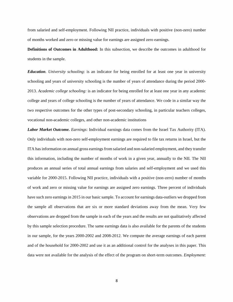
students.9 For example, Table 1 compares the characteristics of treated and comparison students matched

by nearest neighbor matching.10 A total of 1,168 students from comparison schools were matched with

1,789 treated students. We were able to find a match for every treated student. The matched comparison

students were selected from all comparison schools, reinforcing the argument that treated and comparison

schools have similar characteristics. The comparison of treated and matched students shows no significant

differences between the two groups in any of the student or school covariates.

To identify the program effects on non-treated students, we applied the same methodology described

for treated students. Non-treated students in treated schools are compared to students from comparison

schools, using linear regressions and the alternative matching methods.

4.2 Descriptive Statistics

The first year of the study (1999–2000) was a pilot in which only twelfth-grade students from a few

schools participated. Therefore, the evaluation focuses on students who were in 12th grade during the first

year in which the program was fully operational, 2000–2001. Thus, 1998–99 is considered a pretreatment

year. Online appendix Table A2 (reproduced from Lavy and Schlosser 2005) presents the treated

population, 1,789 students which accounted for 28% of all 12th grade students in the treated schools.

However, this rate varied across schools, from 11% to 79%, as a result of a rule that allowed each school

to include up to 100 students in the program irrespective of school size. Although this rule was not strictly

enforced, it led to a negative correlation between the proportion enrolled in the program and school size

9 See Abadie and Cattaneo (2018) for a survey of econometric methods for program evaluation and a useful

comparison of matching/propensity score models with other methods. 10 We first limited the sample to those treated and control students having propensity scores in the region of common

support. Each treated student was matched with a student from comparison schools that had the nearest propensity

score. Some comparison students were matched to more than one treated student. Nevertheless, most comparison

students were used a maximum of two times.

14

(see online appendix Figure A1, reproduced from Figure 2 in Lavy and Schlosser 2005). Online appendix

Figure A2 (reproduced from Figure 4 Lavy and Schlosser 2005) show the relationship between the

preprogram school matriculation rate and the program participation rate. Clearly the figure shows that there

was no correlation between the program participation rate and the preprogram school matriculation rate.

Schools and students were not chosen randomly to participate in the program. However, the gradual

implementation of the program offers a natural comparison group that includes schools that enrolled in the

program at a later year (2001–02). Therefore, we base the identification strategy on a comparison of treated

and untreated students from early and late enrolled schools into the program. The mean characteristics of

the schools that enrolled later strongly resemble those of the schools that enrolled first. Since this similarity

is found both for the pretreatment cohort of seniors and for the treated cohort, it provides support for our

claim that, during the first few years of the program, schools were enrolled in no particular order. Online

appendix Table A3 (appeared as Table 2 in Lavy and Schlosser 2005) presents descriptive statistics and

balancing tests based on data for the 1999 graduating cohort among two groups of schools: schools that

were treated in the first year of the program (col. 1) and schools to be enrolled in the second year (col. 2).

The table shows only a few minor differences between treated and comparison schools. These differences

are presented in column 3 and in parenthesis we present the standard errors. Table 1 presents an equivalent

analysis to table A3 but is based on the 2001 graduating cohort. We discuss these results in more detail in

the next section and we only highlight here the same similarity between treated and comparison schools

that we observed based on the pre-treatment baseline sample of the 1999 cohort. For the 2001 graduating

cohort of Table 1, it is also worth emphasizing the lack of significant differences in terms of lagged

achievements (number of credits earned before twelfth grade and average score), which suggests that

students from treated and comparison schools had similar achievements before the program started. On the

other hand, the comparison of the treated schools with all other high schools in the country (i.e., those that

are neither treated nor comparison schools) reveals a very different pattern. Results not shown in the paper

clearly reveal that the two groups are significantly different in almost all student characteristics. Student

15

achievements during the pretreatment period were also considerably higher in this sample of other schools

than in treated schools.

4.3 Propensity Score and Treated-Comparison Group Comparison

Table 1, columns 1-2, presents detailed summary descriptive statistics for the variables that we use

in the propensity score estimation, by treated students and their matched counterparts which we use as a

comparison group. In column 3 we present the respective mean differences and in parenthesis the

differences standard errors. Panel A presents evidence for student’s demographic characteristics. Mean

mother and father years of schooling are perfectly balanced, the differences being very small (-0.18 and -

0.12) and not statistically different from zero. This pattern of close similarity between the two groups is

also evident for the number of siblings, immigration status, and gender. In panel B we report this sort of

balancing tests for parental average annual earnings in 2000-2002 and their ethnic origin. Father average

annual earnings in this period is 101,363 NIS in the treated group and 98,340 NIS in the comparison group,

the difference of 3,022 NIS is small and not statistically different from zero. Similar evidence is seen for

mother’s annual earnings, and there are no significant differences in parental ethnic origin as well. We note

that data on parental earnings were not available when we studied the effect of the program on short term

outcomes and therefore the treatment-control group balancing evidence is additional support for the close

similarity between the treatment group and the chosen control group.

In panel C we present evidence on lagged schooling outcomes, the average score in matriculation

exams taken prior to 12th grade and number of credits gained through these exams. These two outcomes are

perfectly balanced. For example, the difference between the two groups in lagged average test scores is

0.84 is about one percent of the treatment group mean and is not statistically different from zero. Panel D

includes means of two school characteristics which we include in the propensity score regression,

enrollment in 12th grade and enrollment in 10th through 12th grades. The first of the two is better balanced

with a very small treat-comparison group difference, but in both measures the difference is not statistically

different from zero.

16

4.4 Extensions of Estimation Effect of Remedial Education on High School Outcomes

In this section we present estimates of the program on end of high school matriculation diploma

status. The first row of Table 2 presents estimates based on a specification that includes family earnings as

an additional control variable in the Bagrut outcome regression. As noted above, the family income variable

was not available at the time when Lavy and Schlosser (2005) studied the effect of the program on the

Bagrut rate. We note, however, that adding these family income variables as controls leaves the results

unchanged. In columns 1-3 we present the treatment effect estimates on program participants and in

columns 4-6 we present the (placebo) effect of the program on non-participants from schools that

participated in the program. Columns 1 and 4 present OLS estimates, columns 2 and 5 present nearest

neighbor matching estimates and columns 3 and 6 present kernel matching estimates. In addition to

evidence based on the full sample of participants and non-participants, we also add evidence based on

stratifying the sample by median parental income in the years 2002-2002. Evidence by this sample division

were not reported in Lavy and Schlosser (2005) and therefore they are new evidence presented in this paper.

Several broad conclusions can be drawn from the evidence presented in Table 2. First, using family

income in the propensity score regression does not change the result that the program increased the

matriculation rate of participants by 13 percentage points. Similarly, the zero effect on non-participants is

unchanged as a result of this addition. Secondly, remedial education led to an increase in matriculation rates

of the two sub groups defined by family income but the strongest estimated effect is on the below median

family income students. The program effect on Bagrut rate of this group (panel B) increased by 20

percentage points, about 42 percent increase relative to the ex-post mean of 46 percent of the control group.

The effect on students with family income above the mean is significantly lower, as it is only 5-6 percentage

points relative to an ex-post mean of 65 percent. It could be that students with above median family income

could afford private tutoring, a very common practice towards the high stake matriculation exams, reducing

the effectiveness of additional remedial instruction in school, while those below median could not afford

such private tutoring.

17

5. Effect of Remedial Education on Long Term Outcomes

5.1 Post-Secondary Schooling

We first examine the effect of the remedial education program on post-secondary schooling

attainment. Table 3 presents the treatment effect on ever enrollment and on completed years of schooling

on any type of post-secondary education. In each panel we also present the means of outcome variables for

the treated group. We report estimates based on an OLS regression and on the two different methods of

propensity score matching, nearest neighbor and kernel. All regressions include the original covariates used

in Lavy and Schlosser (2005) and in addition also average family income in the years 2000-2002. Estimates

without this additional control are very similar and therefore we report only the estimates with this control

included. We present estimates of treatment effect on program participants (columns 1-3) for 2013, twelve

years since high school graduation. Similarly, for non-participants, in columns 4-6.

The point estimates in the different columns of Table 3 are consistently similar across the three

methods of estimation. The OLS and the two propensity score matching methods yield positive treatment

effects on ever enrollment and on years of post-secondary schooling. For example, based on kernel

matching, ever enrollment in post-secondary schooling in 2013 is up by a statistically significant 7.6

percentage points (SE=1.9) and the estimates based on the other two methods are 7.2 percent (OLS) and

8.1 percent (nearest neighbor). The effect on completed years of schooling based on kernel matching is

positive and precisely measured, an effect of 0.227 years (se=0.089).

We also use the same three estimation strategies based on a sample of non-participant students and

their matched comparison group and obtain very different results that suggest zero and statistically

insignificant effects of the program on non-participant students in schools that participated in the program.

These estimates which are presented in Table 3 columns 4-6 can be viewed as placebo treatment effects11

though we can also see them as suggesting zero spillover effects within schools. The kernel matching

11 We can frame the analysis for nonparticipants as a placebo analysis. Of course it is not a perfectly clean placebo

since there may be spillovers to the nonparticipants, but the small estimates for non-participants strikes us as

compelling evidence that the estimates for program participants are causal effects.

18

estimate of the effect on post-secondary schooling ever enrollment in 2013 is -0.007 (se=0.017) and

importantly it is statistically different than the estimated effect on the treated. The kernel matching estimate

of the effect on years of post-secondary schooling is 0.064 (se=0.074) and it is also statistically different

then the respective treatment effect on the treated presented in column 3. Both of these placebo estimates

also assure that our estimates are not driven by any school level confounders.

The overall effect on post-secondary schooling can be derived from different effects on the various

types of post-secondary education institutions. Since the program was targeted to relatively underachieving

students we expect to find some effect also through schools that do not confers academic degrees such as

vocational and other non-academic colleges. Table 4 presents estimations of the treatment effect on

completed years of schooling by various types of post-secondary education. The first type, shown in panel

B, includes the seven research universities in Israel that confer BA, MA and PhD degrees. The second sub-

sector is made up of more than 50 academic colleges that mostly confer a BA degree and predominantly

offer social sciences, business and law degrees. The remainder sub-sectors are: teachers' academic colleges,

vocational non-academic colleges, and other non-academic institutions. Table 4 suggests that the positive

effect on post-secondary education is mainly due to increased enrollment and years of schooling in non-

university post-secondary schooling. The effect is largest and most significant on attainment in academic-

colleges. These institutions in Israel are similar to 4-years community colleges in the US. The effect on

completed years of academic college is positive and significant under all three methods. Completed years

of academic college education increased by about a fifth of a year and this change is precisely measured (t

statistic over 4). Relative to a mean of 1.047 for the control group in 2013, these results suggest an effect

of approximately 20% increase. The respective effect on schooling in teachers, vocational and other

institutions are also positive but small and not precisely measured.

The fact that the effects are concentrated on the lower end of the quality of academic education in

Israel is perhaps expected since participants in the remedial education program are at the margin of passing

the matriculation exams and obtaining a bagrut diploma and therefore they are also likely marginal in

admission to post-secondary institutions, especially at one of the seven research universities where

19

admission criterions are much higher. Furthermore, it is interesting to note that the evidence presented in

Table 4 suggest a decline in years of university education of about 0.085 of a year of schooling. This implies

that the program led to some change in the composition of post-secondary schooling, away from the higher

quality university schooling into other, somewhat less lucrative, post-secondary institutions. Several

possible explanations for this result. First, students that improve their average matriculation score can now

choose more desired fields of study but in colleges and not in universities, for example law and business

administration, and they might prefer it over a field of study at a university that they would have chosen

otherwise, for example in humanities or social science. Second, this could be a consequence of peer effect,

for example the students who are affected by the program and as a result get to attend post-secondary

schooling, perhaps ‘pool’ their friends to attend academic colleges instead of universities that they would

have attended otherwise.

In Figures 1-6, we measure the treatment effect for each year since high school graduation and trace

the dynamic pattern for each of the university and college schooling outcomes. To do so, we run a separate

regression for each of the outcomes and for each of the years since high school graduation. We then plot

the coefficients of these regressions around a 90% confidence interval. Note that both the ever-enrolled

variable and the years of schooling are cumulative variables.

We find that the effect on academic colleges ever enrollment rate is flat after six years. This pattern

likely reflects the fact that students who do not enroll in post-secondary schooling in the first six years are

unlikely to return to school later in life. In contrast, the effect on years of schooling accumulates over time.

Most of the increase happens in the first six years and there are very minor changes after 12 years since

graduation. However, the fact that the increase is spread over several years after high school graduation

suggests that measuring outcomes too close to high-school graduation might underestimate the long-term

effects.

The substitution over time from university into academic colleges can be seen graphically in

Figures 4 and 5. The divergence starts early on, suggesting differences in the initial choice of academic

20

institutions and it accumulate over time as students spend time in these institutions. By year 12 after high

school graduation, treated students had accumulated on average 0.2 extra years of academic college

education and 0.085 less years of university education than the control group.

As noted earlier, the remedial education program led also to a positive treatment effect on post-

secondary schooling in other forms of post-secondary schooling. These gains follow the same dynamic

pattern and timing as the gains in academic college education, reaching a pick in the increase in completed

years in teachers’ colleges increased by 0.06 at year 11-12 after high school graduation and an increase in

non-academic schooling and vocational years of schooling of 0.025 each earlier on.

Heterogeneity of Effect of Remedial Education by Socio-Economic Background of Students: The full

sample results might be masking heterogeneous effects by economic background of students. Such

heterogeneity in treatment effect is relevant in this context for understanding the policy implications of our

findings, in particular for considerations of targeting the remedial education treatment to sub-populations

that can mostly benefit from it. In section 4.4 we reported much larger effect on the matriculation rate of

students from families with below median family income and below we present results on the effect on

post-secondary schooling again by stratifying the sample by family income. As noted earlier, we use

average parental income in 2000-2002 as the measure of family income. In columns 4-5 of Table 4 we

report estimates based on samples stratified by family income. Students with below median family income

experienced an increase of 0.3 years in total post-secondary education, compared to their matched control

group. This effect is coming from marginally significant increases of 0.17 and 0.09 years of education in

academic college and teachers’ colleges respectively. In the subgroup with above median family income

we observe a gain of 0.2 years in academic college education and a decrease of 0.16 in university years of

education, both are precisely measured and therefore no gain for this group’s overall post-secondary

schooling attainment.

5.2 Effect on Employment and Earnings

21

We start with a graphical presentation of the dynamic impact of the remedial education program

on labor market outcomes: Earnings, Employment and Months worked. For each outcome we present

estimates from the two different methods of propensity score matching which we use. The labor market

outcomes' data are available until 2015.

Figures 7 and 7A present the estimated effect on employment based on the nearest neighbor and

kernel matching propensity score, respectively. The estimates for the first three years are not meaningful

because most of the students in our sample were still in military service. In the fourth year after high school

graduation, about 90 percent of the individuals in the sample were employed (according to our definition

of employment, which is employed at least for one month during the year and had positive earnings). For

almost all years the estimates are not precisely measured with the exception of 2006, 2010 and 2015 where

the estimates are positive, 2%, 2.3% and 1.7% respectively, and they are statistically significant. These

imprecise and inconclusive employment dynamics imply that they do not play an important role in

determining the effect of the remedial education program on earnings. We gain further insight about the

employment effect of the program by estimating its effect on the total number of months worked in a year.

These estimates are presented in Figures 8 and 8A and they are positive and significant throughout most of

the period. Ignoring the first three years, the estimates for 2006 to 2012 are between 0.2 and 0.3 of a month.

In 2013-2015 the estimates are smaller and no longer statistically different from zero. The small or zero

effect on annual employment status is probably due to a ceiling effect given the high employment rate in

Israel and in our sample as well throughout this period. The positive effect of the program on months of

work suggest that the program increased the likelihood of keeping a job once employed. However, our data

does not allow to test this hypothesis.

We next turn to the time series of estimated effects on annual earnings, which are presented in

Figures 9 and 9A. These treatment estimates are positive throughout the period. They increase over time

monotonically with the exception of 2009 and 2013. Similarly, average annual earnings in the sample also

increase monotonically until the end of the period, from NIS 33,000 (about $8,000) in 2005 to just below

22

NIS 90,000 in 2015. The estimated treatment effects in 2012 and in 2015 (nearest neighbor and kernel) are

significantly different from zero at the 10 percent level and are around 3,400 to 4,000 NIS. In the rest of

the period the treatment effect on earnings is positive and of similar magnitude but it is less precisely

measured. To improve estimation efficiency, especially given that earnings data are noisier than other

outcomes, we run regressions with stacked data for several years at the later part of the study period. We

present these results in Table 5, using panel data for the four last available years. The estimated effect on

average annual earnings during this four-year period are as follows: the kernel earnings effect estimate is

NIS 2,812 with a standard error of 1,750; the nearest neighbor earnings effect estimate is NIS 3,656 with a

standard error of 1,908. The two estimates are not statistically different and are not precisely estimated

though the former is almost significant at 10 percent level of significant.

Another way of examining how significant are the gains in earnings is to focus on earnings’

percentile rank as an outcome because this is a more stable and less noisy measure than absolute earnings.

It might also capture more reliably the permanent long term effect in the labor market. For example, recent

papers in the intergenerational mobility literature have shown that movements across ranks in the income

distribution are uncorrelated with parental income conditional on rank at age 30 while movements in log

earnings are correlated with parental income conditional on log income at age 30 — in particular, rich

offspring have higher earnings growth, so that age 30 measurements are biased predictors of later-life

earnings. However, the rank forecasts appear to be less biased. For example, Nybom and Stuhler (2017)

show with data from Sweden that the relationship between a child’s income rank and their parental income

rank stabilizes by about age 30; in contrast, the relationship in log earnings is less stable. Chetty et al. (2014)

find a similar pattern in the US tax data, reporting that percentile rank predict well where children of

different economic backgrounds will fall in the income distribution later in life. Using log earnings instead

leads to inferior predictions because of the growth path expansions at the top of the income distribution.

Panel D of Table 5 presents estimates of the effect of the remedial program on percentile rank of earnings,

where the rank is computed separately for each cohort. The estimates are fully consistent with the estimated

23

effects on earnings that are presented in Panel C, being positive but much more precisely estimated. The

program increased the rank in the earning distribution by 2.12 percentiles (nearest neighbor estimate) or by

1.8 percentiles based on the kernel matching.

Turning to the effect on other labor market outcomes, the effect on months of work is positive and

marginally significant and the effect on employment status is also positive though not precisely measured.

The positive effect on these two employment outcomes suggest that increased employment in the extensive

and intensive margin contribute to the increase in earnings and so the latter is not solely due to the increase

in schooling attainment.

In columns 4-6 we present the effect on non-participants’ peers in treated schools. The estimated

effects on the three labor market outcomes of non-participants are smaller than the treatment effect on the

treated and are imprecisely measured.

Heterogeneity of Effect on Labor Outcomes by Socio-Economic Background: The above evidence on the

effect of remedial education raise the important question of which segments in the treated population

benefited most from this effect on earnings and relative rank in the income distribution. In particular, from

a policy perspective, it is important to know if the remedial education program was able to move up the

income and rank of the students who come from the lower socio-economic segment of the studied

population, namely those with below median family income. It is also important to examine if the effect on

labor market outcomes by family income square with the effect on post-secondary schooling. In Table 6,

we present results for the effect of remedial education on labor market outcomes based on two sub-samples,

students above and below median family income. The results are similarly polar to the estimates we

obtained for the effect of remedial education on post-secondary schooling. The sample of students with

below median family income experienced statistically significant increase in earnings and in percentile rank

with less precise positive effects on employment and months worked. The above-median family income

group on the other hand shows no observable gains from the program in any of the four labor market

outcomes. In panel E of Table 6 we present estimates of program effect on two unemployment related

24

outcomes: whether an individual experienced a spell of unemployment in a given year (panel E) and the

amount of unemployment annual benefits received (panel F). The mean unemployment rate in the sample

of individuals with below median income is 11.1 percent and in the sample of above median family income

it is 8.7 percent. The estimates for the two outcomes in both sub-samples are small and not significantly

different from zero.

Considering all evidence presented based on samples by family income, these results suggest that

remedial education was very effective for high school students who are below median socio-economic

status in the sample. This group’s post-secondary schooling attainment improved significantly and so did

their labor market outcomes, in particular employment and earnings. We note that in the context of the

remedial program these students might have been those with high likelihood of failing 2-3 exams while

students in the high income group had difficulties in only 1-2 matriculation subjects.

5.3 Mechanisms for the Effect on Long Run Outcomes

There are several channels through which the program could have affected the aforementioned long-run

outcomes. First, through a direct effect on participants’ human-capital. For example, participants might

have gained better learning habits and a sense of accomplishment, which positively affected their post-

secondary and labor market outcomes.

Next, the program could have affected these long-run outcomes through its effect on earning a

matriculation certificate. A matriculation certificate is a prerequisite in virtually all post-secondary

programs in Israel. In addition, a matriculation certificate is a requirement in many early-career jobs which

do not require a college degree. Thus, the matriculation channel of the program effect on labor market is

twofold. Intuitively, in order to decompose the effect, we need to know the effect of matriculation on post-

secondary outcomes, the labor market returns to a matriculation certificate, and the labor market returns to

the different types of post-secondary schooling. Unfortunately, our research design does not allow getting

25

unbiased estimates for these returns12. Therefore, given the threat of endogeneity, we can only provide some

suggestive and correlative evidence on the importance of each mechanism.

We use the logic of the Sobel-Goodman mediation test to test whether getting a matriculation

certificate is an important pathway for the influence of the program on long term post-secondary and labor

market outcomes13. If this is indeed the case, we should observe a reduction in the coefficient of the program

when adding high school matriculation outcomes as a control in the regression. As similar logic follows

when estimating the mediation effects of post-secondary education on labor outcomes. A recent application

of the procedure can be found in Satyanath et al. (2017). In panel A of Table 7 we show the estimated

treatment effect on our main long-run outcomes, when high-school graduation and post-secondary

outcomes are included as controls in the matching procedure. When high-school graduation controls are

added, the effect on post-secondary ever enrollment falls by 44% and the effect on completed years of post-

secondary education falls by 74%. The effect of the program on earnings goes down by 40% when

controlling for high school graduation. When high-school and post-secondary controls are added, the effect

on earnings falls by 50%. Together, these results suggest that a substantial portion, but not all, of the effect

of the program on long-run outcomes is transmitted by its effect on high-school outcomes. Thus also leaving

room for the mechanisms of a direct effect of the program on human capital and the effects of acceptance

to post-secondary education.

A different way to estimate the possible mechanisms for the effects of the program, is, using the

control sample, to first estimate the returns of receiving a high school matriculation diploma on post-

secondary enrolment and labor market outcomes, and the returns to post-secondary schooling on labor

market outcomes. Then, to estimate whether the program had an effect beyond the effects on matriculation

rates and post-secondary enrolment, given the predicted effects of these outcomes. In panel B of Table 7,

we use the sample of students in control schools to create a prediction formula for each of the long-run

12 We are also unaware of any reliable studies on the direct effect of receiving a matriculation degree on labor market

outcomes in Israel. 13 See Baron and Kenny (1986) for a canonical reference of the Sobel-Goodman test.

26

outcomes and then use our original matching procedure to estimate the effect of the program on the

predicted outcome. The prediction formula includes our baseline controls as well as high-school graduation

controls (column 2), post-secondary controls (column 3), and both high-school and post-secondary controls

(column 4). When we add high-school graduation variables to predict the long-run outcome, we get effects

of the program that are around 46% (for post-secondary ever enrollment), 62% (for the completed years of

post-secondary education) and 45% (for annual earning) of the original estimates. When we use both high-

school graduation and post-secondary controls to predict earnings, we get estimates that are about 50% of

the original estimate. Since there is a large portion of the original effect that is not explained by the predicted

outcomes, this suggests that the program might have had a direct effect on human capital.

To conclude, the analysis in this section suggests that there is evidence that the long-run effect of the

program is driven both by a direct effect of the program on human capital and an indirect effect of the

program through earning a matriculation certificate and acceptance into post-secondary institutions. We

caution once more that this analysis is only suggestive as the high-school graduation and the post-secondary

controls are endogenous.

5.4 Effect on Inter-Generational Mobility

To shed further light on the effect of the program on earnings, in Table 8 we present estimates of

its effect on intergenerational earnings mobility. A significant gain in earnings among treated children

should ‘loosen’ the link between child and parent income, therefore enhancing intergenerational income

mobility. The estimates we present in this table are from a regression of children earnings on parental

earnings. Children’s earnings are measured by the earnings average in 2013-2015 years since treatment and

parental earnings are measured as the average family earnings in 2000-2002, while their treated children

were in high school. We estimate the intergenerational income regressions separately for four different

groups. We first compare the results obtained from the sample of the program participants to those in the

matched control group. Secondly, we replicate this analysis for the samples of non-participants in treated

schools and their control group. We then compare within each pair of samples the estimated

27

intergenerational coefficients and use F tests to test whether they are significantly different. We prefer this

approach over estimating the child-parents’ income relationship while pooling the pair of samples and

allowing the income mobility parameter to vary by group. This approach allows all parameters to be

different for the two groups within each pair and it permits the program effect on intergenerational mobility

to be more transparent.

In columns 1-3 we present estimates for sample of program participants and the control group from

other schools (those who entered the program a year later) and in columns 4-6 we present estimates based

on the sample of the non-participants in treated schools and their control group from other schools. Based

on each sample we estimate three different regressions: in the first we use as variables the log of actual

earnings of children and parents. Therefore, observations with zero child or parental earnings are dropped

from the sample in this regression. In the second row we present a regression with the same specification

but the variables used are residuals from regressions that control for age of parents. Note that all children

are of the same age so there is no need to control for their age. In the second specification the variables we

use are percentile rank of children and family earnings. Here again we report results first by using actual

rank and secondly using parental age-residual rank. We note that the advantage of the rank-rank regressions

is that we do not drop from the sample observations with zero earnings.

A consistent pattern emerges in comparing the respective estimates that we obtain from each pair

of samples. First, we note that all the four estimates that are derived based on program’s participants

(column 1) are much smaller than the estimates obtained from the control group sample (column 2). The

regression estimate of log parental earnings on long term child earnings, noted in this literature as the

elasticity of intergenerational mobility, is 0.048 in the treated group, less than half of the respective estimate

(0.114) in the matched control group and the two are significantly different from each other as shown by

the P value of F-test of difference of these two estimates (presented in column 3).14 The implied difference

14 The magnitude of the intergenerational mobility coefficients in Table 7 for the control group are in the mid-range

of what other studies of intergenerational mobility have found in Israel. The most recent evidence is presented in a

Ministry of Finance working paper (Aloni and Krill 2017) which reports an intergenerational elasticity (IGE) of 0.204,

28

represents a sharp increase in intergenerational mobility. The regression’s estimates when using age-

residual variables reported in the second row are identical to the estimates presented in the first row.

A similar pattern is seen in the intergenerational relationship based on percentile rank (third row of

the table), 0.066 in the treated group and 0.130 in the control group, and a P value for the difference between

these two estimates of 0.073. We note that the rank-rank regression includes the full sample without

dropping observations with zero earnings.

In sharp contrast with the estimates presented in column 1-3, the pairwise comparison among non-

participants yields identical intergenerational mobility estimates. The two log earnings regression

parameters in the first row columns 4-5 are 0.102 and 0.106 (P value for difference of these parameters =

0.875). When controlling for parental age the two estimates are even more similar, 0.106 and 0.108 and the

P value for their difference is 0.923. The two percentile rank regression parameters are 0.139 and 0.140 (P

value for difference of these parameters = 0.957).

In summary, the remedial education program reduced sharply the link between child and parents’

income and allowed the treated children to get on a steeper trajectory of income dynamics relative to their

parents. This evidence strengthens further our claim that the remedial education program led to positive

effect on earnings of participants. Even though the direct estimates on earnings are not too precise, the

statistically positive effect of the program on rank of participants in the earning distribution and the negative

effect of the program on the intergenerational earnings elasticity form convincing evidence that the gains

in the bagrut outcome which led to significant gains in post-secondary schooling, led to an increase in

earnings at adulthood.

5.5 Falsification Tests

a higher estimate than the one we report above, Earlier studies (Beenstock, 2008; Frish & Zussman, 2009) use census

data with administrative earnings records. Beenstock reports a very low IGE estimate (approximately 0.04), and Frish

& Zussman focus on the Jewish population and estimate an IGE of 0.2.

29

The main threat to the identification method we use in this paper is the concern that there are unobserved

factors which affect our outcomes and are correlated with either the assignment of the program to different

schools or the assignment of treatment to students within schools. In other words, our results will not be

valid if the program was administered in schools whose population of students with high propensity to be

targeted by the program was different than the same population in comparison schools.

As mentioned in section 2 and described in table A1, the program was not rolled out in any

particular order. To address the concerns about unobserved differences between participants in treated

schools to their control group in non-participating schools, we perform a falsification test in which we

implement our method on a sample of students from the same schools but who are two years older and thus

were not exposed to the program. If there is a meaningful difference between the students with a high

propensity to be treated in treated schools versus those in control schools, we would expect to see this

difference for previous cohorts as well. Table 9 shows the results of this falsification test. Using our original

propensity score estimation, we match our treated students in 2001 with students from the same schools

who graduated in 1999, these matched students will serve as our placebo treated sample. Next, in order to

identify our placebo control sample of students who graduated from our original control schools in 1999,

we employ two different methods. In the first method we take our 1999 placebo treatment students and

match them with the students who graduated from our original control schools in 1999. In the second

method we use the original treatment propensity formula to directly match the students who were treated

in 2001 with students who graduated from our original control schools in 1999. All estimates for the

differences between the placebo treated and control samples for both methods are, reassuringly, not

significantly different than zero. For example, using the first method, the estimated effect on annual

earnings is 430 NIS with SE of 3,495 while the estimated effect on ever enrolling to post-secondary studies

is -0.04 with SE of 0.037.

6. Conclusions

30

Remedial interventions in high school are under scrutiny in most OECD countries. For example, in

the US the focus is on the cost and place of remediation policies within the higher education system, given

the growing demand for skilled labor (Bettinger and Long 2009, Bettinger and Baker 2011). In England

this debate has gained particular relevance recently given the policy changes that require students who do

not get at least a grade C in English or math in GCSE (mid high school high stake exams) to repeat exams

in these subjects. However, remediation policies are often costly and their efficiency in boosting student

performance has been questioned (Schwartz 2012, Van Effenterre 2017), especially given the limited

evidence on the longer term outcomes. Banerjee et al. (2007), Banerjee et al. (2010) and Banerjee et al.

(2016) discuss remedial education programs and their effectiveness in developing countries, finding

evidence that suggests that targeted remedial interventions can address effectively children’s learning gaps.

In this paper we study a successful remedial education program that improved short term outcomes of under

achieving high school students and examine whether these gains are long lasting and whether the

intervention has a high internal rate of return. We consider several long run outcomes, including

continuation to higher education and subsequent labor market earnings.

The gradual implementation of the program allows us to use a propensity score matching design in

which participants in the program are matched with non-participants from schools that adopted the program

a year later. We combine high school records with National Social Security administrative data to examine

longer-term outcomes when students were in their early 30s. Our evidence suggests that treated students

experienced economically meaningful gains in post-secondary schooling enrollment which increased by

13.7 percent and in completed years of education which increased by 11 percent. These gains were driven

by gains in lower quality tier of academic institutions in Israel, mainly academic and teachers’ colleges,

with no significant change in university schooling. Annual earnings of treated participants increased by 4

percent, partly explained by an increase of 1.5 percent in months employed and the rest accounted by higher

education. The gain in income is also shown in an increase in income mobility among the treated group as

31

compared to the control group. We find significant heterogeneity in these treatment effects, with most of

the gains occurring to students from families with below median family income.

The average cost of the program was $1,100 per participant. Average Yearly added earnings from

program participation around age 30 was about $750. Assuming that participants pay about 20 per cent

income tax rate on these earnings suggest that the government will recover its cost within 7-8 years,

implying a very high rate of return to this remedial education program. Naturally this return depends on

how permanent is the effect on earnings. First, we note that we measure the effect on earnings at about age

30-31, when individuals had already completed their post-secondary schooling. Second, based on a sample

of older cohorts, we find that earnings at age 30-35 is a strong predictor of earnings at an older age. Third,

we estimated also a significant effect on percentile rank of individuals in the distribution of their cohort, a

measure believed to be a more stable predictor of later life earnings (Nybom and Stuhler 2017, Chetty et al

2014). A note of caution is warranted however as this cost-benefit comparison is not taking into account

possible general equilibrium consideration that might reduce the rate of return to schooling when remedial

education is expanded at scale.

7. References

Abadie, Alberto, and Matias D. Cattaneo. 2018. Econometric methods for program

evaluation. Annual Review of Economics 10 (1): 465–503.

Abadie, Alberto, and Guido W. Imbens. 2011. Bias-corrected matching estimators for average

treatment effects. Journal of Business & Economic Statistics: A Publication of the American Statistical

Association 29 (1): 1–11.

Angrist, Joshua D. 1998. Estimating the labor market impact of voluntary military service using

social security data on military applicants. Econometrica 6, no. 2:249–88.

32

Angrist, Joshua, Daniel Lang, and Philip Oreopoulos. 2009. Incentives and services for college

achievement: Evidence from a randomized trial. American Economic Journal. Applied Economics 1 (1):

136–63.

Angrist, Joshua, and Victor Lavy. 2009. The effects of high stakes high school achievement awards:

evidence from a randomized trial. The American Economic Review 99 (4): 1384–1414.

Abadie, Alberto, and Guido W. Imbens.2002. Simple and bias-corrected matching estimators for

average treatment effects. No. t0283. National Bureau of Economic Research, 2002.

Aloni, Tslil, and Zeev Krill. 2017. Intergenerational income mobility in Israel—international and

sectoral comparisons. Ministry of Economics, Office of Chief Economist.

Banerjee, Abhijit V., Shawn Cole, Esther Duflo, and Leigh Linden. 2017. "Remedying education:

Evidence from two randomized experiments in India. The Quarterly Journal of Economics 122, no. 3:1235-

1264.

Banerjee, Abhijit, Rukmini Banerji, James Berry, Esther Duflo, Harini Kannan, Shobhini Mukherji,

Marc Shotland, and Michael Walton. 2016. Mainstreaming an effective intervention: Evidence from

randomized evaluations of ‘Teaching at the Right Level’ in India. NBER Working Paper 22746, National

Bureau of Economic Research, Cambridge, MA.

Banerjee, Abhijit V., Rukmini Banerji, Esther Duflo, Rachel Glennerster, and Stuti Khemani. 2010.

Pitfalls of participatory programs: Evidence from a randomized evaluation in education in India. American

Economic Journal: Economic Policy 2, no. 1: 1-30.

Banerjee, Abhijit V., Shawn Cole, Esther Duflo, and Leigh Linden. 2007. Remedying education:

Evidence from two randomized experiments in India. The Quarterly Journal of Economics 122, no. 3:1235-

1264.

33

Baron, Reuben M., and David A. Kenny. 1986. The moderator–mediator variable distinction in

social psychological research: Conceptual, strategic, and statistical considerations. Journal of personality

and social psychology 51, no. 6: 1173.

Battistin, Erich, and Antonio Schizzerotto. 2012. Threat of grade retention, remedial education and

student achievement: Evidence from upper secondary schools in Italy. IZA DP No. 7086.

Beenstock, Michael. 2008. Deconstructing the sibling correlation: How families increase

inequality. Journal of family and economic issues 29, no. 3: 325-345.

Eric, Bettinger, and Rachel Baker. 2011. The Effects of Student Coaching in College: An

Evaluation of a Randomized Experiment in Student Mentoring. NBER Working Paper 16881, National

Bureau of Economic Research, Cambridge, MA.

Bettinger, Eric P., and Bridget Terry Long. 2009. Addressing the needs of underprepared students

in higher education does college remediation work? Journal of Human resources 44, no. 3: 736-771.

Calcagno, Juan Carlos, and Bridget Terry Long. 2008. The impact of postsecondary remediation

using a regression discontinuity approach: Addressing endogenous sorting and noncompliance. NBER

Working Paper 14194. National Bureau of Economic Research, Cambridge, MA.

Chetty, Raj, Nathaniel Hendren, Patrick Kline, and Emmanuel Saez. 2014. Where is the land of

opportunity? The geography of intergenerational mobility in the United States. The Quarterly Journal of

Economics 129, no. 4: 1553-1623.

Currie, Janet. 2001. Early childhood education programs. The Journal of Economic Perspectives:

A Journal of the American Economic Association 15 (2): 213–38.

Currie, Janet, and Thomas Duncan. 2001. Early test scores, school quality and SES: Long run

effects on wage and employment outcomes. In Worker wellbeing in a changing labor market, ed. Polachek,

Solomon. Research in labor economics. Emerald group publishing limited.

34

Davison, Antony C., and David Hinkley. 1997. Bootstrap methods and their application.

Cambridge: Cambridge University Press.

Dynarski, Mark, and Philip Gleason. 2002. How can we help? What we have learned from recent

federal dropout prevention evaluations. Journal of Education for Students Placed at Risk, 7(1): 43–69.

Frish, Roni, and Noam Zussman. 2009. The Causal Effect of Parents' Childhood Environment and

Education on Their Children's Education. Bank of Israel discussion paper 2009.02. Bank of Israel.

Garces, Eliana, Duncan Thomas, and Janet Currie. 2002. Longer-term effects of head start. The

American Economic Review 92 (4): 999–1012.

Heckman, James, and Pedro Carneiro. 2003. Human capital policy. NBER Working Paper 9495.

National Bureau of Economic Research, National Bureau of Economic Research, Cambridge, MA.

Krueger, Alan B., and Diane M. Whitmore. 2001. The effect of attending a small class in the early

grades on college-test taking and middle school test results: evidence from project STAR. The Economic

Journal 111 (468): 1–28.

Imbens, Guido W. 2004. Nonparametric estimation of average treatment effects under exogeneity:

A review. Review of Economics and statistics 86, no. 1: 4-29.

Lavy, Victor. 2002. Evaluating the effect of teachers’ group performance incentives on pupil

achievement. Journal of Political Economy 110, no. 6:1286–1317.

———. 2009. Performance Pay and Teachers’ Effort, Productivity, and Grading Ethics. The

American Economic Review 99 (5): 1979–2011.

Lavy, Victor, & Schlosser, Analia. 2005. Targeted Remedial Education for Underperforming

Teenagers: Costs and Benefits. Journal of Labor Economics, 23(4), 839–874.

35

Leuven, Edwin, and Barbara Sianesi. 2003. PSMATCH2: Stata module to perform full

Mahalanobis and propensity score matching, common support graphing, and covariate imbalance testing.

Martorell, Paco, and Isaac McFarlin Jr. 2011. Help or hindrance? The effects of college remediation

on academic and labor market outcomes. The Review of Economics and Statistics 93, no. 2: 436-454.

Ministry of Education, Culture, and Sport. 2001. Facts and figures about education in Israel.

Jerusalem: Publications Department, Ministry of Education, Culture, and Sport.

Nybom, Martin, and Jan Stuhler. 2017. Biases in standard measures of intergenerational income

dependence. Journal of Human Resources 52, no. 3:800-825.

Robins, James M., and Ya'acov Ritov. 1997. Toward a curse of dimensionality appropriate (CODA)

asymptotic theory for semi‐parametric models. Statistics in medicine 16, no. 3:285-319.

Rosenbaum, Paul R., and Donald B. Rubin. 1983. The central role of the propensity score in

observational studies for causal effects. Biometrika 70, no. 1:41–55.

Satyanath, Shanker, Nico Voigtländer, and Hans-Joachim Voth. 2017. Bowling for fascism: Social

capital and the rise of the Nazi Party. Journal of Political Economy 125, no. 2:478-526.

Schwartz, Analice C. Remedial Education Programs to accelerate learning for All. World Bank,

2012.

Scrivener, Susan, Michael J. Weiss, Alyssa Ratledge, Timothy Rudd, Colleen Sommo, and Hannah

Fresques. 2015. Doubling Graduation Rates: Three-Year Effects of CUNY’s Accelerated Study in

Associate Programs (ASAP) for Developmental Education Students. SSRN Scholarly Paper ID 2571456.

Rochester, NY: Social Science Research Network.

Smith, Jeffrey A., and Petra E. Todd. 2005. Does matching overcome LaLonde’s critique of

nonexperimental estimators? Journal of Econometrics 125 (1): 305–53.

36

Subramanian, Shankar, and Angus Deaton. 1996. The demand for food and calories. Journal of

Political Economy 104, no. 1:133–62.

Van Effenterre Clémentine. 2017. Post 16 remedial policies: a literature review. Centre for

Vocational Educational Research London School of Economics & Political Science, Research Discussion

Paper 005.

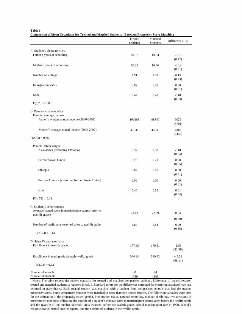
37

Treated

Students

Matched

StudentsDifference (1-2)

A. Student’s characteristics

Father’s years of schooling 10.37 10.54 -0.18

(0.42)

Mother’s years of schooling 10.63 10.76 -0.12

(0.51)

Number of siblings 2.51 2.38 0.13

(0.23)

Immigration status 0.02 0.02 0.00

(0.01)

Male 0.42 0.43 -0.01

(0.03)

F(5,73) = 0.03

B. Parental characteristics

Parental average income

Father’s average annual income (2000-2002) 101363 98340 3022

(8701)

Mother’s average annual income (2000-2002) 47537 45730 1807

(3435)

F(2,73) = 0.25

Parents’ ethnic origin

Asia-Africa (excluding Ethiopia) 0.32 0.33 -0.01

(0.04)

Former Soviet Union 0.20 0.21 0.00

(0.05)

Ethiopia 0.02 0.02 0.00

(0.01)

Europe-America (excluding former Soviet Union) 0.06 0.06 0.00

(0.01)

Israel 0.40 0.39 0.01

(0.04)

F(4, 73) = 0.13

C. Student’s achievements

Average lagged score in matriculation exams (prior to

twelfth grade)73.43 72.59 0.84

(0.90)

Number of credit units received prior to twelfth grade 6.84 6.84 0.00

(0.38)

F(2, 73) = 1.14

D. School’s characteristics

Enrollment in twelfth grade 177.65 179.51 -1.86

(21.56)

Enrollment in tenth grade through twelfth grade 544.34 589.92 -45.58

(68.11)

F(2,73) = 6.32

Number of schools 40 34

Number of students 1789 1168

Table 1

Comparison of Mean Covariates for Treated and Matched Students - Based on Propensity Score Matching

Notes.-The table reports descriptive statistics for treated and matched comparison students. Difference of means between

treated and matched students is reported in col. 3. Standard errors for the differences corrected for clustering at school level are

reported in parentheses. Each treated student was matched with a student from comparison schools that had the nearest

propensity score. Some comparison students were matched to more than one treated student. The following variables were used

for the estimation of the propensity score: gender, immigration status, parental schooling, number of siblings, two measures of

pretreatment outcomes indicating the quartile of a student’s average score in matriculation exams taken before the twelfth grade

and the quartile of the number of credit units awarded before the twelfth grade, school matriculation rate in 1999, school’s

religious status, school size, its square, and the number of students in the twelfth grade.

38

OLS

Nearest

Neighbor

Matching

Kernel

MatchingOLS

Nearest

Neighbor

Matching

Kernel Matching

(1) (2) (3) (4) (5) (6)

A. Full Sample

Mean for the treated group

Estimate 0.131*** 0.131*** 0.126*** 0.006 -0.008 -0.005

(0.025) (0.017) (0.015) (0.017) (0.013) (0.011)

B. Below Median Family Income

Mean for the treated group

Estimate 0.172*** 0.195*** 0.193*** 0.009 0.000 -0.003

(0.032) (0.024) (0.021) (0.019) (0.018) (0.016)

C. Above Median Family Income

Mean for the treated group

Estimate 0.091*** 0.056** 0.051** 0.002 -0.013 -0.014

(0.025) (0.023) (0.020) (0.018) (0.018) (0.016)

(0.456) (0.496)

Notes.-The table reports estimated treatment effects on the student matriculation status for program participants (cols. 1–3) and for students that studied in

treated schools but did not participate in the program (cols. 4–6). Columns 1 and 4 present OLS estimates from models that control for student’s and

school’s characteristics. Estimates for cols. 2, 3, 5, and 6 are based on nearest neighbor matching and kernel matching methods and were computed using

Stata procedures developed by Becker and Ichino (2002). The following variables were used for the estimation of the propensity score in each panel:

gender, immigration status, parental schooling, number of siblings, two measures of pretreatment outcomes indicating the quartile of a student’s average

score in matriculation exams taken before the twelfth grade and the quartile of the number of credit units awarded before the twelfth grade, school

matriculation rate in 1999, school’s religious status, school size, its square, the number of students in the twelfth grade and the average family income in

2000-2002. Standard errors (in parentheses) are corrected for clustering at the school level in OLS regressions. Panel A presents the estimation for the

entire sample while in panel B, C, D and E the sample is stratified to students with above median matriculation scores prior to 12th grade and students

below the median, students with family income below median and students with family income above median, respectively. The stratification is carried by

removing the students in treated schools who don't belong to the selected group.

** Significant at the 5% level.

*** Significant at the 1% level.

0.654 0.372

(0.476) (0.484)

0.705 0.561

(0.466) (0.499)

Table 2

Estimates of the Effect of Additional Targeted Individualized Instruction on Bagrut Eligibility

Participants Nonparticipants

0.681 0.465

39

OLS

Nearest

Neighbor

Matching

Kernel

MatchingOLS

Nearest

Neighbor

Matching

Kernel Matching

(1) (2) (3) (4) (5) (6)

Enrollment

Mean for the treated group

Estimate 0.072*** 0.081*** 0.076*** -0.003 -0.008 -0.007

(0.019) (0.021) (0.019) (0.016) (0.017) (0.017)

Years of Schooling

Mean for the treated group

Estimate 0.220** 0.231** 0.227** 0.087 0.046 0.064

(0.093) (0.093) (0.089) (0.074) (0.074) (0.074)

(0.483) (0.500)

Table 3

Estimates of the Effect of Additional Targeted Individualized Instruction on Post Secondary Schooling by 2013

Participants Nonparticipants

0.631 0.508

2.293 1.997

(2.281) (2.452)

Notes.-The table reports estimated treatment effects on the student's post-secondary enrollment and years of schooling for program participants (cols.

1–3) and for students that studied in treated schools but did not participate in the program (cols. 4–6). Columns 1 and 4 present OLS estimates from

models that control for student’s and school’s characteristics. Estimates for cols. 2, 3, 5, and 6 are based on nearest neighbor matching and kernel

matching methods and were computed using Stata procedures developed by Becker and Ichino (2002). The following variables were used for the

estimation of the propensity score are gender, immigration status, parental schooling, number of siblings, two measures of pretreatment outcomes

indicating the quartile of a student’s average score in matriculation exams taken before the twelfth grade and the quartile of the number of credit units

awarded before the twelfth grade, school matriculation rate in 1999, school’s religious status, school size, its square, the number of students in the

twelfth grade and the average family income in 2000-2002. Standard errors (in parentheses) are corrected for clustering at the school level.

** Significant at the 5% level.

*** Significant at the 1% level.

40

OLS

Nearest

Neighbor

Matching

Kernel

MatchingAbove Median Below Median

(1) (2) (3) (4) (5)

A. Post Secondary Schooling

Mean for the treated group 2.564 2.004

(2.274) (2.255)

Estimate 0.220** 0.231** 0.227** 0.145 0.297**

(0.093) (0.093) (0.089) (0.112) (0.124)

B. University Schooling

Mean for the treated group 0.610 0.410

(1.540) (1.304)

Estimate -0.080 -0.075 -0.085 -0.157** 0.004

(0.064) (0.063) (0.055) (0.068) (0.066)

C. College Schooling

Mean for the treated group 1.420 1.065

(1.843) (1.675)

Estimate 0.212*** 0.235*** 0.202*** 0.205** 0.168*

(0.075) (0.086) (0.078) (0.095) (0.094)

D. Teacher Colleges

Mean for the treated group 0.266 0.261

(0.954) (0.939)

Estimate 0.059* 0.060 0.063* 0.032 0.093**

(0.035) (0.040) (0.035) (0.044) (0.044)

E. Vocational Two Year College

Mean for the treated group 0.160 0.170

(0.550) (0.648)

Estimate 0.006 0.026 0.025 0.040 0.008

(0.032) (0.033) (0.032) (0.032) (0.038)

F. Other

Mean for the treated group 0.096 0.090

(0.489) (0.491)

Estimate 0.021 0.029* 0.023 0.019 0.032

(0.016) (0.016) (0.015) (0.020) (0.020)

Number of Observation 7,008 4,326 7,006 3,543 3,462

0.165

(0.599)

0.093

(0.490)

Notes.-The table reports estimated treatment effects on the student's post-secondary years of schooling in a specific type of post-secondary

institution for program participants (cols. 1–3) and for subgroups by ability as measures by matriculation scores prior to 12th grade (cols. 4-5)

and by family income (cols. 6-7). Column 1 present OLS estimates from models that control for student’s and school’s characteristics. Estimates

for Column 2 is based on nearest neighbor matching and Columns 3-6 are based on kernel matching methods and were computed using Stata

procedures developed by Becker and Ichino (2002). The following variables were used for the estimation of the propensity score: gender,

immigration status, parental schooling, number of siblings, two measures of pretreatment outcomes indicating the quartile of a student’s average

score in matriculation exams taken before the twelfth grade and the quartile of the number of credit units awarded before the twelfth grade,

school matriculation rate in 1999, school’s religious status, school size, its square, the number of students in the twelfth grade and the average

family income in 2000-2002. Standard errors (in parentheses) are corrected for clustering at the school level.

* Significant at the 10% level.

** Significant at the 5% level.

*** Significant at the 1% level.

(0.947)

Table 4

Estimates of the Effect of Additional Targeted Individualized Instruction on Years of Schooling by Institution Type and by Groups by

2013Participants By Family Income (Kernel Matching)

2.293

(2.281)

0.514

(1.434)

1.249

(1.772)

0.264

41

OLS

Nearest

Neighbor

Matching

Kernel

MatchingOLS

Nearest

Neighbor

Matching

Kernel Matching

(1) (2) (3) (4) (5) (6)

A. Employmet

Mean for the treated group

Estimate 0.010 0.0131* 0.008 -0.007 -0.007 -0.009

(0.008) (0.008) (0.007) (0.007) (0.007) (0.007)

B. Months Worked

Mean for the treated group

Estimate 0.173** 0.248*** 0.143* -0.096 -0.093 -0.105

(0.088) (0.095) (0.082) (0.080) (0.086) (0.085)

C. Earnings (NIS)

Mean for the treated group

Estimate 3116 3656* 2812 1046 1538 1722

(1958) (1908) (1750) (1358) (1288) (1318)

D. Percentile Ranking of Earnings

Estimate 1.813** 2.122** 1.802** 0.072 0.122 0.375

(0.797) (0.864) (0.751) (0.559) (0.598) (0.578)

Number of Observations 28,016 17,166 28,008 39,286 33,316 39,262

(0.304) (0.327)

Table 5

Estimates of the Effect of Additional Targeted Individualized Instruction on Earnings and Employment, Stacked 2012-2015

Participants Nonparticipants

0.897 0.878

Notes.-The table reports estimated treatment effects on the student's labor market outcomes for program participants (cols. 1–3) and for students that studied in treated

schools but did not participate in the program (cols. 4–6). Columns 1 and 4 present OLS estimates from models that control for student’s and school’s characteristics.

Estimates for cols. 2, 3, 5, and 6 are based on nearest neighbor matching and kernel matching methods and were computed using Stata procedures developed by Becker

and Ichino (2002). The following variables were used for the estimation of the propensity score: gender, immigration status, parental schooling, number of siblings, two

measures of pretreatment outcomes indicating the quartile of a student’s average score in matriculation exams taken before the twelfth grade and the quartile of the

number of credit units awarded before the twelfth grade, school matriculation rate in 1999, school’s religious status, school size, its square, the number of students in the

twelfth grade and the average family income in 2000-2002. Standard errors (in parentheses) are corrected for clustering at the school level.

* Significant at the 10% level.

** Significant at the 5% level.

*** Significant at the 1% level.

9.781 9.488

(3.964) (4.222)

76913 76042

(62927) (70392)

42

Above Median Below Median

(1) (2)

A. Employment

Mean for the treated group 0.899 0.895

(0.301) (0.307)

Estimate -0.003 0.016

(0.010) (0.012)

B. Months Worked

Mean for the treated group 9.860 9.695

(3.910) (4.020)

Estimate -0.023 0.256*

(0.125) (0.142)

C. Earnings (NIS)

Mean for the treated group 82198 71245

(66208) (58691)

Estimate 612 4111*

(2502) (2134)

D. Percentile Ranking of Earnings

Estimate 0.856 2.389**

(1.030) (1.085)

E. Annual Unemployment Insurance Benefits (Binary Indicator)

Mean for the treated group 0.087 0.111

(0.282) (0.314)

Estimate -0.001 0.012

(0.007) (0.008)

F. Annual Unemployment Insurance Benefits (NIS)

Mean for the treated group 969 1179

(3766) (4114)

Estimate -47 116

(79) (90)

Number of Observations 14,176 13,842

Table 6

Estimates of the Effect of Additional Targeted Individualized Instruction on Employment Outcomes By

Ability and Family Income, stacked 2012-2015 - Based on Kernel Matching

By Family Income

Notes.-The table reports the heterogeneous treatment effects on the student's labor market outcome for participants

by matriculations scores prior to 12th grade and by average family income in 2000-2002. Columns 1 thru 4 present

estimates based on kernel matching using Stata procedures developed by Becker and Ichino (2002). The following

variables were used for the estimation of the propensity score: gender, immigration status, parental schooling,

number of siblings, two measures of pretreatment outcomes indicating the quartile of a student’s average score in

matriculation exams taken before the twelfth grade, the quartile of the number of credit units awarded before the

twelfth grade, school matriculation rate in 1999, school’s religious status, school size, its square, the number of

students in the twelfth grade and the average family income in 2000-2002. The stratification to boys and girls was

carried by removing the students in treated schools who don't belong to the selected group. Standard errors (in

parentheses) are corrected for clustering at the school level.

* Significant at the 10% level.

** Significant at the 5% level.

43

High School

Matriculation

Controls

Post

Secondary

Controls

All

Education

Controls

(1) (2) (3)

A. Adding Endogenous Controls

Enrollment in any Post-secondary Institution 12 years after High School Graduation (1 = Yes, 0 = No) 0.043** - -

(0.020)

Completed Years of Post-secondary Schooling 12 years after High School Graduation 0.059

(0.093) - -

Annual Earnings 2012-2015 1,661 2,032 1,399

(1,820) (1,754) (1,801)

B. Effect on Predicted Outcome

Enrollment in any Post-secondary Institution 12 years after High School Graduation (1 = Yes, 0 = No) 0.035*** - -

(0.006)

Completed Years of Post-secondary Schooling 12 years after High School Graduation 0.141***

(0.028) - -

Annual Earnings 2012-2015 1279*** 1220*** 1517***

(250) (291) (328)

Table 7

Effect of Additional Targeted Individualized Instruction when High School and Post-Secondary Educational Outcomes are Added As

Controls in the Propensity Matching Procedure

Notes.-Panel A assesses the sensitivity of the treatment effects presented in tables 2-6 when adding high school and post-secondary educational outcomes as

control in the propensity matching kernel procedure. Panel B assesses the treatment effect on predicted long-run outcomes, where the prediction formula is

estimated only on comparison schools students. Columns 1-3 present the estimated treatment effects when the high school and post-secondary educational

outcome variable mentioned in the column header are controlled for (Panel A) or are used in estimating the outcome prediction formula (Panel B). High school

controls in column 1 include a dummy variable for matriculation and average matriculation score. Post-secondary controls in column 2 include a dummy for

enrollment to post-secondary institution and years of post-secondary schooling. Standard errors are clustered at the school level. Number of observations in post-

secondary regressions is 7,005 and the number of observations in annual earnings regressions is 28,012.

* Significant at the 10% level.

** Significant at the 5% level.

*** Significant at the 1% level.

Added Control Variables

44

Treated

Group

Control

Group

P-Value for Differences

Between Groups

(Chi Square in Parentheses)

From Treated

Schools

Control

Group

P-Value for Differences

Between Groups

(Chi Square in Parentheses)

(1) (2) (3) (4) (5) (6)

Paternal Earnings (Avg. 2000-2002)

Log Earnings (IGE) 0.049*** 0.109*** 0.037 0.102*** 0.106*** 0.875

(0.019) (0.023) (4.357) (0.014) (0.019) (0.025)

Log Earnings (IGE) (Residuals on Age) 0.048** 0.114*** 0.028 0.106*** 0.108*** 0.923

(0.019) (0.024) (4.819) (0.014) (0.019) (0.009)

Percentile Ranking 0.066*** 0.130*** 0.073 0.139*** 0.140*** 0.957

(0.026) (0.025) (3.207) (0.015) (0.020) (0.003)

Percentile Ranking (Residuals on Age) 0.071*** 0.135*** 0.069 0.143*** 0.144*** 0.977

(0.025) (0.025) (3.314) (0.015) (0.020) (0.001)

Number of Observations 1,435 4,036 3,590 4,036

Table 8

Estimates of the Effect of Additional Targeted Individualized Instruction on Earning Mobility Outcomes Based on Kernel Matching

Individual Earnings (Avg. 2013-2015)

Participants Non Participants

Notes.-The table reports the differences between the treated and matched control groups in estimated earning mobility as measured by regressing parental earnings

on individual earnings. We exclude individuals that have 0 as their or the father's avg. earnings. Columns 1-2 and 4-5 present regression estimates of the average

income of the fathers of the students in our sample in 2000-2002 on the individual earnings of the students in 2013-2015. Columns 1 displays results for the treated

group and column 2 presents results for the matched control group based on kernel matching using Stata procedures developed by Becker and Ichino (2002).

Column 4 presents results for students that studied in treated schools but did not participate in the program and column 5 the results for their matched control group

using kernel matching. Columns 3 and 6 present the p value and the Chi squared of the test comparing the mobility coefficient between the treated and control

groups. The following variables were used for the estimation of the propensity score: gender, immigration status, parental schooling, number of siblings, two

measures of pretreatment outcomes indicating the quartile of a student’s average score in matriculation exams taken before the twelfth grade, the quartile of the

number of credit units awarded before the twelfth grade, school matriculation rate in 1999, school’s religious status, school size, its square, the number of students in

the twelfth grade and the average family income in 2000-2002. Standard errors (in parentheses) are corrected for clustering at the school level.

* Significant at the 10% level.

** Significant at the 5% level.

*** Significant at the 1% level.

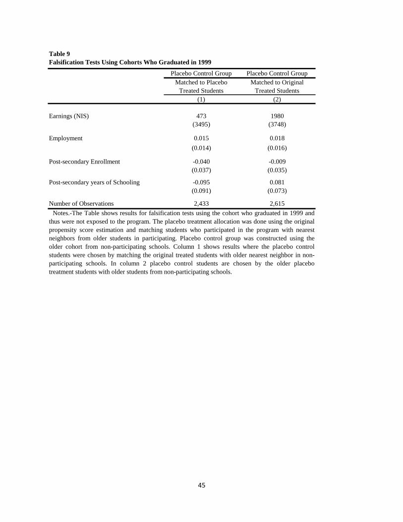
45

Placebo Control Group Placebo Control Group

Matched to Placebo

Treated Students

Matched to Original

Treated Students

(1) (2)

Earnings (NIS) 473 1980

(3495) (3748)

Employment 0.015 0.018

(0.014) (0.016)

Post-secondary Enrollment -0.040 -0.009

(0.037) (0.035)

Post-secondary years of Schooling -0.095 0.081

(0.091) (0.073)

Number of Observations 2,433 2,615

Table 9

Falsification Tests Using Cohorts Who Graduated in 1999

Notes.-The Table shows results for falsification tests using the cohort who graduated in 1999 and

thus were not exposed to the program. The placebo treatment allocation was done using the original

propensity score estimation and matching students who participated in the program with nearest

neighbors from older students in participating. Placebo control group was constructed using the

older cohort from non-participating schools. Column 1 shows results where the placebo control

students were chosen by matching the original treated students with older nearest neighbor in non-

participating schools. In column 2 placebo control students are chosen by the older placebo

treatment students with older students from non-participating schools.

46

-0.2

-0.1

0

0.1

0.2

0.3

0.4

0.5

0.6

0.7

0.8

-0.04

-0.02

0

0.02

0.04

0.06

0.08

0.1

0.12

0.14

0.16

2002 2003 2004 2005 2006 2007 2008 2009 2010 2011 2012 2013

Ever

En

rollm

en

t R

ate

Ever

En

rollm

en

t R

ate

Years

Figure 1: Mean and Treatment Effect: Any Post-Secondary Schooling Ever Enrollment (Nearest Neighbor)

Treatment Effect Estimate

Mean for Treated

*Shaded area indicates two sided confidence intervals, 10% significance level.

47

-0.2

-0.1

0

0.1

0.2

0.3

0.4

0.5

0.6

0.7

0.8

-0.04

-0.02

0

0.02

0.04

0.06

0.08

0.1

0.12

0.14

0.16

2002 2003 2004 2005 2006 2007 2008 2009 2010 2011 2012 2013

Ever

En

rollm

en

t R

ate

Ever

En

rollm

en

t R

ate

Years

Figure 1A: Mean and Treatment Effect: Any Post-Secondary Schooling Ever Enrollment (Kernel Matching)

Treatment Effect Estimate

Mean for Treated

*Shaded area indicates two sided confidence intervals, 10% significance level.

48

-0.18

-0.15

-0.12

-0.09

-0.06

-0.03

0

0.03

0.06

0.09

0.12

0.15

0.18

-0.04

-0.03

-0.02

-0.01

0

0.01

0.02

0.03

0.04

2002 2003 2004 2005 2006 2007 2008 2009 2010 2011 2012 2013

Ever

En

rollm

en

t R

ate

Ever

En

rollm

en

t R

ate

Years

Figure 2: Mean and Treatment Effect: University Ever

Enrollment (Nearest Neighbor)

Treatment Effect Estimate

Mean for Treated

*Shaded area indicates two sided confidence intervals, 10% significance level.

49

-0.18

-0.15

-0.12

-0.09

-0.06

-0.03

0

0.03

0.06

0.09

0.12

0.15

0.18

-0.04

-0.03

-0.02

-0.01

0

0.01

0.02

0.03

0.04

2002 2003 2004 2005 2006 2007 2008 2009 2010 2011 2012 2013

Ever

En

rollm

en

t R

ate

Ever

En

rollm

en

t R

ate

Years

Figure 2A: Mean and Treatment Effect: University Ever Enrollment (Kernel Matching)

Treatment Effect Estimate

Mean for Treated

*Shaded area indicates two sided confidence intervals, 10% significance level.

50

-0.2

-0.1

0

0.1

0.2

0.3

0.4

0.5

0.6

-0.04

-0.02

0

0.02

0.04

0.06

0.08

0.1

0.12

2002 2003 2004 2005 2006 2007 2008 2009 2010 2011 2012 2013

Ever

En

rollm

en

t R

ate

Ever

En

rollm

en

t R

ate

Years

Figure 3: Mean and Treatment Effect: College Ever Enrollment (Nearest Neighbor)

Treatment Effect Estimate

Mean for Treated

*Shaded area indicates two sided confidence intervals, 10% significance level.

-0.2

-0.1

0

0.1

0.2

0.3

0.4

0.5

0.6

-0.04

-0.02

0

0.02

0.04

0.06

0.08

0.1

0.12

2002 2003 2004 2005 2006 2007 2008 2009 2010 2011 2012 2013

Ever

En

rollm

en

t R

ate

Eve

r En

rollm

en

t R

ate

Years

Figure 3A: Mean and Treatment Effect: College Ever Enrollment (Kernel Matching)

Treatment Effect Estimate

Mean for Treated

*Shaded area indicates two sided confidence intervals, 10% significance level.

51

-0.5

0

0.5

1

1.5

2

2.5

-0.1

0

0.1

0.2

0.3

0.4

0.5

2002 2003 2004 2005 2006 2007 2008 2009 2010 2011 2012 2013

Ye

ars

of

Sch

oo

ling

Ye

ars

of

Sch

oo

ling

Years

Figure 4: Mean and Treatment Effect: Any Post-Secondary Years of Schooling (Nearest Neighbor)

Treatment Effect Estimate

Mean for Treated

*Shaded area indicates two sided confidence intervals, 10% significance level.

-0.5

0

0.5

1

1.5

2

2.5

-0.1

0

0.1

0.2

0.3

0.4

0.5

2002 2003 2004 2005 2006 2007 2008 2009 2010 2011 2012 2013

Ye

ars

of

Sch

oo

ling

Ye

ars

of

Sch

oo

ling

Years

Figure 4A: Mean and Treatment Effect: Any Post-Secondary Years of Schooling (Kernel Matching)

Treatment Effect Estimate

Mean for Treated

*Shaded area indicates two sided confidence intervals, 10% significance level.

52

-0.6

-0.4

-0.2

0

0.2

0.4

0.6

-0.25

-0.2

-0.15

-0.1

-0.05

0

0.05

0.1

0.15

0.2

0.25

2002 2003 2004 2005 2006 2007 2008 2009 2010 2011 2012 2013

Ye

ars

of

Sch

oo

ling

Ye

ars

of

Sch

oo

ling

Years

Figure 5: Mean and Treatment Effect: University Years of Schooling (Nearest Neighbor)

Treatment Effect Estimate

Mean for treated

*Shaded area indicates two sided confidence intervals, 10% significance level.

-1

-0.8

-0.6

-0.4

-0.2

0

0.2

0.4

0.6

0.8

1

-0.2

-0.15

-0.1

-0.05

0

0.05

0.1

0.15

0.2

2002 2003 2004 2005 2006 2007 2008 2009 2010 2011 2012 2013

Ye

ars

of

Sch

oo

ling

Ye

ars

of

Sch

oo

ling

Years

Figure 5A: Mean and Treatment Effect: University Years of Schooling (Kernel Matching)

Treatment Effect Estimate

Mean for treated

*Shaded area indicates two sided confidence intervals, 10% significance level.

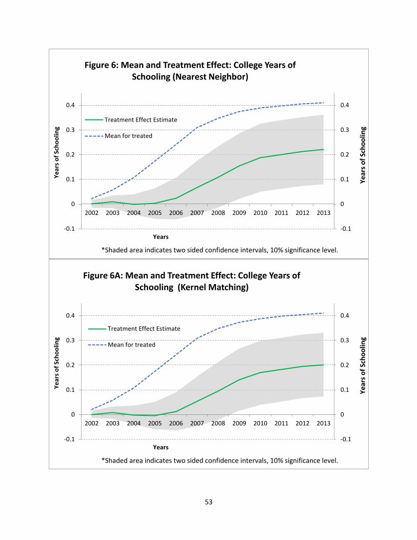
53

-0.1

0

0.1

0.2

0.3

0.4

-0.1

0

0.1

0.2

0.3

0.4

2002 2003 2004 2005 2006 2007 2008 2009 2010 2011 2012 2013

Ye

ars

of

Sch

oo

ling

Ye

ars

of

Sch

oo

ling

Years

Figure 6: Mean and Treatment Effect: College Years of Schooling (Nearest Neighbor)

Treatment Effect Estimate

Mean for treated

*Shaded area indicates two sided confidence intervals, 10% significance level.

-0.1

0

0.1

0.2

0.3

0.4

-0.1

0

0.1

0.2

0.3

0.4

2002 2003 2004 2005 2006 2007 2008 2009 2010 2011 2012 2013

Ye

ars

of

Sch

oo

ling

Ye

ars

of

Sch

oo

ling

Years

Figure 6A: Mean and Treatment Effect: College Years of Schooling (Kernel Matching)

Treatment Effect Estimate

Mean for treated

*Shaded area indicates two sided confidence intervals, 10% significance level.

54

-1

-0.8

-0.6

-0.4

-0.2

0

0.2

0.4

0.6

0.8

1

-0.06

-0.04

-0.02

0

0.02

0.04

0.06

2002 2003 2004 2005 2006 2007 2008 2009 2010 2011 2012 2013 2014 2015

Years

Figure 7: Mean and Treatment Effect: Employment Rate (Nearest Neighbor)

Treatment Effect

Mean for treated

*Shaded area indicates two sided confidence intervals, 10% significance level.

55

-1

-0.8

-0.6

-0.4

-0.2

0

0.2

0.4

0.6

0.8

1

-0.06

-0.04

-0.02

0

0.02

0.04

0.06

2002 2003 2004 2005 2006 2007 2008 2009 2010 2011 2012 2013 2014 2015

Years

Figure 7A: Mean and Treatment Effect: Employment Rate (Kernel Matching)

Treatment Effect

Mean for treated

*Shaded area indicates two sided confidence intervals, 10% significance level.

56

-12

-9

-6

-3

0

3

6

9

12

-0.8

-0.6

-0.4

-0.2

0

0.2

0.4

0.6

0.8

2002 2003 2004 2005 2006 2007 2008 2009 2010 2011 2012 2013 2014 2015

Years

Figure 8: Mean and Treatment Effect: Months Worked(Nearest Neighbor)

Treatment Effect

Mean for treated

*Shaded area indicates two sided confidence intervals, 10% significance level.

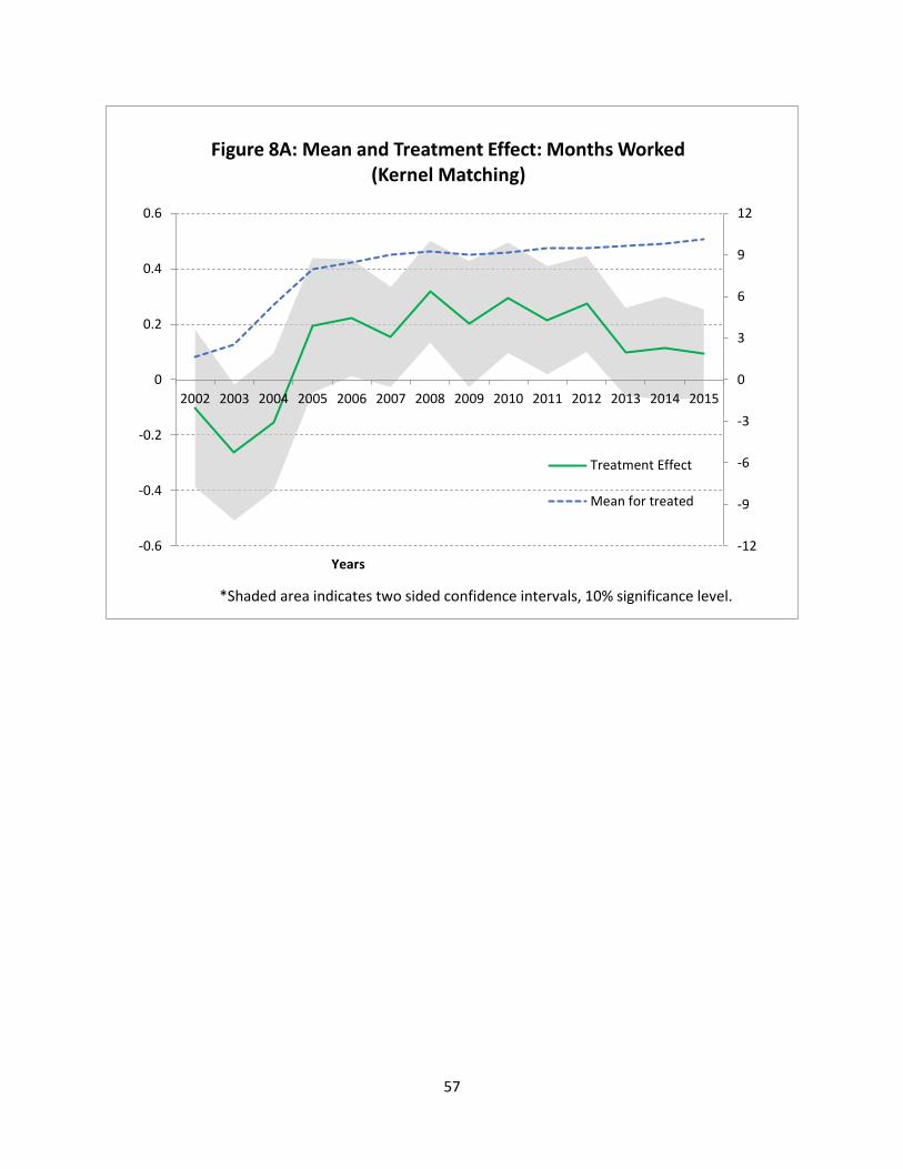
57

-12

-9

-6

-3

0

3

6

9

12

-0.6

-0.4

-0.2

0

0.2

0.4

0.6

2002 2003 2004 2005 2006 2007 2008 2009 2010 2011 2012 2013 2014 2015

Years

Figure 8A: Mean and Treatment Effect: Months Worked (Kernel Matching)

Treatment Effect

Mean for treated

*Shaded area indicates two sided confidence intervals, 10% significance level.

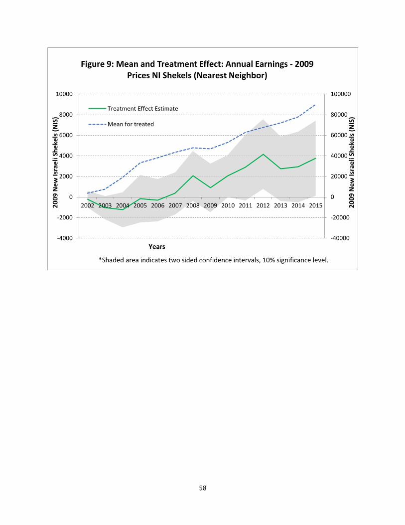
58

-40000

-20000

0

20000

40000

60000

80000

100000

-4000

-2000

0

2000

4000

6000

8000

10000

2002 2003 2004 2005 2006 2007 2008 2009 2010 2011 2012 2013 2014 2015 20

09

New

Isra

eli S

hek

els

(NIS

)

20

09

New

Isra

eli S

hek

els

(NIS

)

Years

Figure 9: Mean and Treatment Effect: Annual Earnings - 2009 Prices NI Shekels (Nearest Neighbor)

Treatment Effect Estimate

Mean for treated

*Shaded area indicates two sided confidence intervals, 10% significance level.

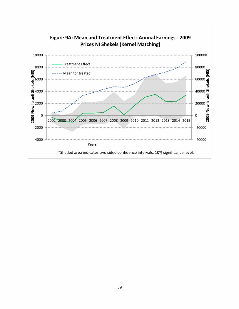
59

-40000

-20000

0

20000

40000

60000

80000

100000

-4000

-2000

0

2000

4000

6000

8000

10000

2002 2003 2004 2005 2006 2007 2008 2009 2010 2011 2012 2013 2014 2015 20

09

New

Isra

eli S

hek

els

(NIS

)

20

09

New

Isra

eli S

hek

els

(NIS

)

Years

Figure 9A: Mean and Treatment Effect: Annual Earnings - 2009 Prices NI Shekels (Kernel Matching)

Treatment Effect

Mean for treated

*Shaded area indicates two sided confidence intervals, 10% significance level.