formulation of consistent finite volume schemes for...
TRANSCRIPT

Full Terms & Conditions of access and use can be found athttps://www.tandfonline.com/action/journalInformation?journalCode=tjhr20
Journal of Hydraulic Research
ISSN: 0022-1686 (Print) 1814-2079 (Online) Journal homepage: https://www.tandfonline.com/loi/tjhr20
Formulation of consistent finite volume schemesfor hydraulic transients
Sara Mesgari Sohani & Mohamed Salah Ghidaoui
To cite this article: Sara Mesgari Sohani & Mohamed Salah Ghidaoui (2019) Formulation ofconsistent finite volume schemes for hydraulic transients, Journal of Hydraulic Research, 57:3,353-373, DOI: 10.1080/00221686.2018.1522377
To link to this article: https://doi.org/10.1080/00221686.2018.1522377
Published online: 20 Dec 2018.
Submit your article to this journal
Article views: 102
View Crossmark data
Journal of Hydraulic Research Vol. 57, No. 3 (2019), pp. 353–373https://doi.org/10.1080/00221686.2018.1522377© 2018 International Association for Hydro-Environment Engineering and Research
Research paper
Formulation of consistent finite volume schemes for hydraulic transientsSARA MESGARI SOHANI, Graduate MPhil Student, Civil Department, Hong Kong University of Science and Technology, HongKong, PR ChinaEmail: [email protected] (author for correspondence)
MOHAMED SALAH GHIDAOUI (IAHR Member), Chinese Estates Professor of Engineering and Chair Professor CivilDepartment, Hong Kong University of Science and Technology, Hong Kong, PR ChinaEmail: [email protected]
ABSTRACTIntentionally generated transient waves are used in the detection of defects in pipelines. Experience to date in these applications shows that the widerthe band of injected wave frequencies the better is the detection effectiveness. Thus, as these technologies develop further, models that can handle highfrequency waves will be required. Finite volume (FV) methods are well suited for high frequency wave phenomena, but their use in the water hammerfield has been limited to date compared with other fields such as open channel flow. A major reason for this is that FV methods are formulated forsimple boundary conditions such as no-flux or no-slip, but have not been well developed for the typically more complex boundary conditions found inpressurized pipeline systems (e.g. junctions, control valves, orifices, tanks and reservoirs). In those few instances in the literature where FV has beenapplied to water hammer problems, the approach has been to use FV for internal sections and method of characteristics (MOC) at the boundaries.The global order of accuracy of FV–MOC is governed by the MOC solution. To our knowledge, this paper constitutes a first attempt at handlingboundary conditions within the FV framework. The approach places the boundary element within a FV to enforce mass and momentum conservationwithin this volume. The fluxes between the FV and the adjacent elements are then formulated in the usual manner. The approach is illustrated for thecase of a valve, a reservoir and a junction. The finite volume method used is the Boltzmann-type scheme. The accuracy and efficiency of all schemeswith the proposed non-iterative FV formulation of the boundary conditions are demonstrated through the following test cases: (i) water hammerwave interactions with a junction boundary characterized by a geometric discontinuity, (ii) water hammer wave interactions with a junction boundarycharacterized by a discontinuity in the value of wave speed, and (iii) water hammer wave interactions with a junction characterized by a flow ratediscontinuity. The pure FV formulation guarantees mass and momentum conservation. The Boltzmann-based FV schemes capture discontinuity aswell as wave interactions with boundary elements accurately. The stability of the proposed FV schemes is satisfied when Cr < 0.5.
Keywords: Boltzmann method; boundary condition; finite volume; high frequency wave; water hammer
1 Introduction
Pressurized pipeline systems are key infrastructure in the water,oil, and gas industries. These systems transport fluids fromsource to treatment and from treatment to point(s) of con-sumption. In addition to the pipe components themselves, thesesystems include a large number of devices (e.g. valves, pumpsand tanks) whose role is to move, store or control flow and pres-sure and to maintain them at desired levels. These devices aredistinguishable from the pipes by their small length scale incomparison to the length scale of pipes. As a result, the tradi-tional approach to solving the flow equation in a pipe is to treatthe devices as localized boundary conditions (Chaudhry, 1979;Karney, 1984).
Sudden flow disturbances caused either accidentally or delib-erately by these devices or boundary conditions can trigger fast,large, and even destructive waves that propagate throughout thepipe system and continually interact with devices. From thestructural integrity point of view, engineers need to estimatehow large the potential amplitude of critical generated pressurewaves is in both the negative (pressure decrease) and positive(pressure increase) sense. Extreme positive pressure waves cancause catastrophic system failure , e.g. the Russian hydroelectricplant disaster (Hasler, 2010). Extreme negative pressure wavescan lead to cavitation-induced failures (Siemons, 1967) and mayincrease the cross-contamination risk through nearby cracksor pipeline joints (Ebacher, Besner, Prévost, & Allard, 2010;LeChevallier, Gullick, Karim, Friedman, & Funk, 2003).
Received 31 July 2016; accepted 7 September 2018/Open for discussion until 31 December 2019.
ISSN 0022-1686 print/ISSN 1814-2079 onlinehttp://www.tandfonline.com
353

354 S. Mesgari Sohani and M.S. Ghidaoui Journal of Hydraulic Research Vol. 57, No. 3 (2019)
Moreover, the occurrence of transient waves in water sup-ply systems may also adversely affect the quality of drinkingwater since sudden flow changes also may cause sedimentand biofilm detachment, leading to discoloration and loss ofresidual chlorine (Aisopou, Stoianov, & Graham, 2010). Otherpossible impacts of transient waves include excessive noise,fatigue, pitting due to cavitation, disruption of normal control,and a destructive resonant vibration associated with the inherentperiod of certain pipe systems.
Not all transient pressure waves are bad. Research conductedin the past 20 years shows that planned and controlled tran-sient waves are beneficially used in the detection of defectssuch as leakage and blockage in pipelines without disruptiveaccess to the pipe network. Defects such as leakages, which area major and widespread problem in pressurized pipe systems,contribute roughly 30% to water loss in water supply systems(Thornton, Sturm, & Kunkel, 2008). The detection attributes oftransient waves are: (i) rapidity, since they propagate at speedsof 400–1000 m s−1; (ii) efficiency, since they contain a wealth ofinformation on all parts of the system through which they prop-agate; and (iii) non-destructiveness, since they do not requiresystem alteration. The signature of different defects on tran-sient waves can be rapidly collected using a finite number oflocations (e.g. access-points to pipe networks) and can be usedto extract and identify defect parameters in a post-processingstep (Brunone, 1999; Duan, Lee, Ghidaoui, & Tung, 2012;Liou, 1998; Mohapatra, Chaudhry, Kassem, & Moloo, 2006;Stephens, Lambert, Simpson, Vítkovsky, & Nixon, 2004).
While research in the past 20 years has showed significantpotential of transient-based detection methods, only recentlyhas the importance of high frequency waves and model accu-racy to defect detection been pointed out (Duan et al., 2012;Stephens et al., 2004). Therefore, it would seem imperativethat the numerical models used have a higher order of accu-racy. Among the many numerical methods applied to transients(e.g. method of characteristics (MOC), wave plan (WP), finitedifference (FD), finite element (FE), finite volume (FV), andcorrective smoothed particle method (CSPM)), FV methodsare known to be well suited for high frequency waves (Luo& Xu, 2013; Luo, Xuan, & Xu, 2013). However, FV meth-ods have traditionally been formulated only for simple boundaryconditions such as the Neumann, Dirichlet or Robin conditions.FV methods have not been formulated for the more complex andubiquitous types of boundary conditions that are present in pipesystems such as valves, junctions and pumps. Such boundaryconditions are generally in the form of pressure-flow relationsthat are nonlinear, implicit, time-dependent and not renderedeasily amenable to the FV framework.
Conventionally, these boundary conditions are straightfor-wardly handled in the MOC framework by defining the mathe-matical expressions to relate pressure head and discharge. MOCwas first applied to water hammer by Streeter and Lai (1962).Streeter and Wylie (1967) extended MOC to handle bound-ary conditions for a few simple systems. Chaudhry (1968,
1979) developed boundary conditions for reservoirs, sprinklers,valves, surge tanks and air chambers. Karney (1984) devel-oped an algorithm to perform comprehensive transient analysisof networks with arbitrary complexity in which he presentsconcise terminology for describing pipe networks and bound-ary conditions. McInnis (1993) formulated a unified set ofboundary conditions that handles devices and layouts that arefound in practical water supply systems. Axworthy (1997)developed boundary conditions that are consistent with quasi-steady state, rigid water column, and water hammer theories.These developments led to comprehensive treatment of var-ious boundary conditions such as valves, pumps, turbines,accumulators, air valves and many others and helped cementthe key role of MOC in engineering practice. In fact, Ghi-daoui, Zhao, McInnis, and Axworthy (2005) reported that11 out of 14 commercially available water hammer soft-ware packages are based on MOC. Comprehensive treatmentof various boundary conditions can be found in researchpapers written by Streeter and Wylie (1967), Wylie, Streeter,and Suo (1993), Karney (1984), Chaudhry (1968), Chaudhryand Hussaini (1985), McInnis (1993), Axworthy (1997). How-ever, in spite of all the advantages of MOC, MOC is problematicwhere the wave speed variation is large, due to presence ofair or wall thinning. MOC, also, cannot be easily extendedto two-dimensional and three-dimensional models because thecharacteristic relationships are not lines but become surfaces ofcones and surfaces of spheres, respectively.
The treatment of boundary conditions in FV methodology isnot straightforward. Guinot (1998) used a high-order, mono-tonic numerical scheme of the Godunov method to simulatewater hammer waves in a FV framework. He proposed nineoptions to handle boundary conditions in a reservoir-pipe-valvesystem, and only one combination among the nine is shownto provide good results. Conventionally, a junction boundary istreated using either an iterative or non-iterative method to guar-antee a single value of pressure and momentum at the junction(Chae, Lee, Hwang, & Lee, 2006; Kriel, 2012). Guinot (1998)also suggested an iterative treatment for the junction boundaryconditions. Often, where FV has been applied to water hammerproblems, the approach has been to use FV for internal sectionsand MOC at the boundaries (Zhao & Ghidaoui, 2004). SuchFV–MOC hybridization means that the global order of accuracyis governed by the scheme with the lowest order of accuracy,which is invariably the MOC solution. The order of accuracy ofthe MOC solution degrades due to discretization problems thatrise when modeling multi-pipe systems.
A non-iterative FV method for junction boundary treat-ment was developed by Hong and Kim (2011). A ghost junc-tion cell was implemented while considering linear momen-tum interchange and wall effects. In their proposed model theRoeM scheme (i.e. the modified Roe scheme Kim, Kim, Rho,& Hong, 2003) is used to conserve mass and momentum and,at the same time, the stagnation enthalpy across the geometricdiscontinuity is preserved. In particular, their attempt to simulate
Journal of Hydraulic Research Vol. 57, No. 3 (2019) Formulation of consistent finite volume 355
wave–system interactions at a junction characterized by a geom-etry discontinuity was flawed. Their numerical results differfrom the analytical solutions and involve significant overshootsand undershoots. The origin of this discrepancy is likely due tothe way they enforce enthalpy conservation.
The major driving force behind the current study is the needfor a pure FV numerical model suitable for (i) high frequencywaves and (ii) high wave speed variation. Note that not all FVschemes are suitable for high frequency waves. For instance,Louati (2013) pointed that a two-dimensional Riemann-basedfinite volume scheme numerically dissipates high frequencywaves for transient flow in pipes. The mesoscopic-basedschemes used in the current study can be easily extended to anon-dissipative model of order three or higher (Luo & Xu, 2013;Luo et al., 2013).
In the next section, the numerical implementations of bound-ary conditions are developed within a Boltzmann-based finitevolume approach.
2 Governing equations
In the finite volume approach, the integral formulation of themass and momentum conservation laws is applied on a physicalspace as follows (Hirsch, 2007):
∂
∂t
∫CV
[ρ
ρu
]d –V +
∮CS
[ρu
ρu2 + P
]· �s dA = q (1)
where CV denotes control volume; CS denotes control surface;ρ is the density; A is the area; –V is the volume; u is the flowvelocity in x-direction which is equal to the average flow veloc-ity in x-direction (i.e. U) in the current one-dimensional waterhammer model; �s is the outward normal unit vector (perpendic-ular to surface area); q is designated sink/source terms, and Pis the pressure. For gas flow problems, P is coupled with flowdensity and temperature through the gas flow state equation. Inwater hammer, however, temperature is decoupled from pres-sure due to relatively large specific heat of water. Thus, the stateequation fitted for water hammer applications is dP/dρ = a2,where a is transient wave speed (Chaudhry, 1979). The time-dependent mass and momentum fluxes on the control surfacecan be obtained after integrating Eq. (1) with respect to t. The
time-dependent mass and momentum fluxes denotedMassF and
MomF , respectively are:
⎡⎣Mass
FMomF
⎤⎦ =
∫ [ρu
ρu2 + P
]dt (2)
Mesgari Sohani and Ghidaoui (2018) successfully formu-lated the second-order Bhatnagar–Gross–Krook (BGK) and thekinetic flux vector splitting (KFVS) schemes for a classicalreservoir-pipe-valve water hammer test case in a finite vol-ume framework. They calculated time-dependent fluxes on
surface volumes using Boltzmann-based equations. In order tocompare the classical water hammer solution to the proposedunified finite volume scheme, a map suggested by MesgariSohani and Ghidaoui (2018) to relate ρ and ρu to H and Q isrepresented below:
H = ρa2
9.81ρ0, Q = ρUA
ρ0(3)
where ρ0 is the density before any disturbance, and A is the pipecross-sectional area. Using the map, the numerical results asso-ciated with the KFVS and BGK schemes can be representedin the form of pressure head, notwithstanding that the originalgoverning equations solve density and mass flux. In the cur-rent paper all fluxes (i.e. at pipes and boundaries) are calculatedusing the BGK and KFVS schemes to solve transient wavesinside pipes.
It is worth mentioning that in the classical water hammermodel, wave speed includes both water and pipe wall effects inthe formulation (Chaudhry, 1979), whereas in the mesoscopic-based approaches, wave speed only bears the elasticity of fluidand excludes the wall effects (i.e. the rigid pipe assumption). Inother words, the mesoscopic-based models solve fluid in pipesand exclude any interaction between fluid and pipe wall. Toinclude the wall elasticity in the current formulation, however,the mesoscopic-based models are able to adopt the wall elas-ticity effect as external forces in formulation. Such a practiceis out of the scope of the current study and is left for futurestudies.
3 Numerical schemes
In the one-dimensional water hammer framework, Eq. (1)is traditionally applied to the flow inside a pipe (Zhao& Ghidaoui, 2004) and auxiliary relations are used at thedevices. In this paper, Eq. (1) is enforced everywhere in the pipesystem, where a device is contained within a control volume(CV). The fluxes between the CV that contains the boundaryelement and the adjacent cells are then formulated using a FVmethod. In the current paper the finite volume methods used arethe BGK and KFVS methods (i.e. mesoscopic-based methods)formulated by Mesgari Sohani and Ghidaoui (2018) for a clas-sical water hammer test case and are extended to moderatelycomplex pipe network systems.
Figure 1a sketches a pipe network including the boundaryelements (e.g. valve, junction, reservoir and pump) and defects(e.g. leak, blockage and thinning wall). In Fig. 1b, all bound-ary elements are replaced with CVs indicated by the red colour,and defects (i.e. a sort of boundary condition) are replaced withpurple-coloured CVs. The CV is able to take different geome-tries into account but is a lumped representation of a boundarycondition and does not provide the flow details within it.
The one-dimensional representation of the unified FVmethod is illustrated in Fig. 2a for a simple pipe network with no

356 S. Mesgari Sohani and M.S. Ghidaoui Journal of Hydraulic Research Vol. 57, No. 3 (2019)
Figure 1 (a) Pipe network with boundary elements and defects. (b) The conceptual model to handle boundary conditions
Figure 2 (a) Schematic of a pipe network with boundary elements. (b) Discrete space domain in pipes and control volumes associated with controlelements. (c) The unified FV approached in a discrete space
friction but with boundary elements such as a junction, a valveand a reservoir. The number of pipes and elements are denotedby NP and NE , respectively. The length of elements, generally,is quite small in comparison with the length scale of pipes (i.e.δk′/Lk � 1, where k ∈ [1, NP]; k′ ∈ [1, NE]; Lk is the length ofpipe k; and δk′ is the length of element k′).
Figure 2b shows a discrete space domain in which all pipesare uniformly discretized, so �xk = Lk/Nk, where k ∈ [1, NP];Nk is the number of cells in pipe k; and�xk is the cell size in pipek. For such a multi-pipe system, the number of numerical cellsin the entire computational domain is the sum of Nk where k ∈[1, NP] and is denoted by Nx. Geometrically flexible CVs shown
Journal of Hydraulic Research Vol. 57, No. 3 (2019) Formulation of consistent finite volume 357
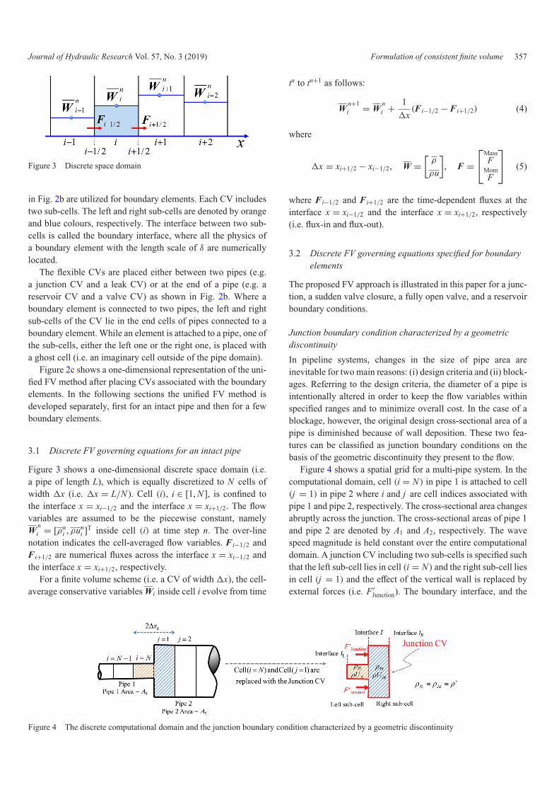
Figure 3 Discrete space domain
in Fig. 2b are utilized for boundary elements. Each CV includestwo sub-cells. The left and right sub-cells are denoted by orangeand blue colours, respectively. The interface between two sub-cells is called the boundary interface, where all the physics ofa boundary element with the length scale of δ are numericallylocated.
The flexible CVs are placed either between two pipes (e.g.a junction CV and a leak CV) or at the end of a pipe (e.g. areservoir CV and a valve CV) as shown in Fig. 2b. Where aboundary element is connected to two pipes, the left and rightsub-cells of the CV lie in the end cells of pipes connected to aboundary element. While an element is attached to a pipe, one ofthe sub-cells, either the left one or the right one, is placed witha ghost cell (i.e. an imaginary cell outside of the pipe domain).
Figure 2c shows a one-dimensional representation of the uni-fied FV method after placing CVs associated with the boundaryelements. In the following sections the unified FV method isdeveloped separately, first for an intact pipe and then for a fewboundary elements.
3.1 Discrete FV governing equations for an intact pipe
Figure 3 shows a one-dimensional discrete space domain (i.e.a pipe of length L), which is equally discretized to N cells ofwidth �x (i.e. �x = L/N ). Cell (i), i ∈ [1, N ], is confined tothe interface x = xi−1/2 and the interface x = xi+1/2. The flowvariables are assumed to be the piecewise constant, namelyW
ni = [ρn
i , ρuni ]T inside cell (i) at time step n. The over-line
notation indicates the cell-averaged flow variables. Fi−1/2 andFi+1/2 are numerical fluxes across the interface x = xi−1/2 andthe interface x = xi+1/2, respectively.
For a finite volume scheme (i.e. a CV of width �x), the cell-average conservative variables Wi inside cell i evolve from time
tn to tn+1 as follows:
Wn+1i = W
ni + 1
�x(Fi−1/2 − Fi+1/2) (4)
where
�x = xi+1/2 − xi−1/2, W =[ρ
ρu
], F =
⎡⎣Mass
FMomF
⎤⎦ (5)
where Fi−1/2 and Fi+1/2 are the time-dependent fluxes at theinterface x = xi−1/2 and the interface x = xi+1/2, respectively(i.e. flux-in and flux-out).
3.2 Discrete FV governing equations specified for boundaryelements
The proposed FV approach is illustrated in this paper for a junc-tion, a sudden valve closure, a fully open valve, and a reservoirboundary conditions.
Junction boundary condition characterized by a geometricdiscontinuity
In pipeline systems, changes in the size of pipe area areinevitable for two main reasons: (i) design criteria and (ii) block-ages. Referring to the design criteria, the diameter of a pipe isintentionally altered in order to keep the flow variables withinspecified ranges and to minimize overall cost. In the case of ablockage, however, the original design cross-sectional area of apipe is diminished because of wall deposition. These two fea-tures can be classified as junction boundary conditions on thebasis of the geometric discontinuity they present to the flow.
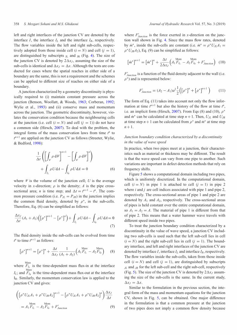
Figure 4 shows a spatial grid for a multi-pipe system. In thecomputational domain, cell (i = N ) in pipe 1 is attached to cell(j = 1) in pipe 2 where i and j are cell indices associated withpipe 1 and pipe 2, respectively. The cross-sectional area changesabruptly across the junction. The cross-sectional areas of pipe 1and pipe 2 are denoted by A1 and A2, respectively. The wavespeed magnitude is held constant over the entire computationaldomain. A junction CV including two sub-cells is specified suchthat the left sub-cell lies in cell (i = N ) and the right sub-cell liesin cell (j = 1) and the effect of the vertical wall is replaced byexternal forces (i.e. F ′
Junction). The boundary interface, and the
Figure 4 The discrete computational domain and the junction boundary condition characterized by a geometric discontinuity
358 S. Mesgari Sohani and M.S. Ghidaoui Journal of Hydraulic Research Vol. 57, No. 3 (2019)
left and right interfaces of the junction CV are denoted by theinterface I , the interface IL and the interface IR, respectively.The flow variables inside the left and right sub-cells, respec-tively adopted from those inside cell (i = N ) and cell (j = 1),are distinguished by subscripts JL and JR (Fig. 4). The size ofthe junction CV is denoted by 2�xJ , assuming the size of thesub-cells is identical and�xJ = �x. Although the tests are con-ducted for cases where the spatial reaches in either side of aboundary are the same, this is not a requirement and the schemescan be applied to different size of reaches on either side of aboundary.
A junction characterized by a geometry discontinuity is phys-ically required to (i) maintain constant pressure across thejunction (Benson, Woollatt, & Woods, 1963; Corberan, 1992;Wylie et al., 1993) and (ii) conserve mass and momentumacross the junction. The geometric discontinuity, however, vio-lates the conservation condition because the neighbouring cellsat the junction (i.e. cell (i = N ) and cell (j = 1)) do not havea common side (Hirsch, 2007). To deal with the problem, theintegral forms of the mass conservation laws from time tn totn+1 are applied on the junction CV as follows (Streeter, Wylie,& Bedford, 1998):
1�t
([∫–Vρ d –V
]n+1
−[∫
–Vρ d –V
]n)
+∫
IL
ρU dA −∫
IR
ρU dA = 0 (6)
where –V is the volume of the junction cell; U is the averagevelocity in x-direction; ρ is the density; A is the pipe cross-sectional area; n is time step; and �t = tn+1 − tn. The com-mon pressure condition (i.e. PJL = PJR) in the junction impliesthe common fluid density, denoted by ρ∗, in the sub-cells.Therefore, Eq. (6) can be simplified as follows:
�xJ
�t(A1 + A2)
([ρ∗]n+1 − [
ρ∗]n)+∫
IL
ρU dA−∫
IR
ρU dA= 0
(7)
The fluid density inside the sub-cells can be evolved from timetn to time tn+1 as follows:
[ρ∗]n+1 = [
ρ∗]n + �t�xJ
1(A1 + A2)
(A1
MassFIL − A2
MassFIR
)(8)
whereMassFIL is the time-dependent mass flux-in at the interface
IL; andMassFIR is the time-dependent mass flux-out at the interface
IR. Similarly, the momentum conservation law is applied to thejunction CV and gives:
([ρ∗UJLA1 + ρ∗UJRA2
]n+1 − [ρ∗UJLA1 + ρ∗UJRA2
]n)�xJ
�t
= A1MomFIL − A2
MomFIR + F ′
Junction (9)
where F ′Junction is the force exerted in x-direction on the junc-
tion wall shown in Fig. 4. Since the mass flow rates, denotedby m∗, inside the sub-cells are constant (i.e. m∗ = ρ∗UJLA1 =ρ∗UJRA2), Eq. (9) can be simplified as follows:
[m∗]n+1 = [
m∗]n + �t2�xJ
(A1
MomFIL − A2
MomFIR + F ′
Junction
)(10)
F ′Junction is a function of the fluid density adjacent to the wall (i.e.ρ∗) and is represented below:
F ′Junction = (A2 − A1)a2 1
2
([ρ∗]n + [
ρ∗]n+1)
(11)
The form of Eq. (11) takes into account not only the flow infor-mation at time tn+1 but also the history of the flow at time tn,i.e. an implicit form (Hirsch, 2007). From Eqs (8) and (10), ρ∗
and m∗ can be calculated at time step n + 1. Then, UJL and UJR
at time step n + 1 can be calculated from ρ∗ and m∗ at time stepn + 1.
Junction boundary condition characterized by a discontinuityin the value of wave speed
In practice, when two pipes meet at a junction, their character-istics such as material or thickness may be different. The resultis that the wave speed can vary from one pipe to another. Suchvariations are important in defect detection methods that rely onfrequency shifts.
Figure 5 shows a computational domain including two pipes,which is uniformly discretized. In the computational domain,cell (i = N ) in pipe 1 is attached to cell (j = 1) in pipe 2where i and j are cell indices associated with pipe 1 and pipe 2,respectively. The cross-sectional areas of pipe 1 and pipe 2 aredenoted by A1 and A2, respectively. The cross-sectional areasof pipes is held constant over the entire computational domain,so A1 = A2 = A. The material of pipe 1 is different from thatof pipe 2. This means that a water hammer wave travels withdifferent speed inside two pipes.
To treat the junction boundary condition characterized by adiscontinuity in the value of wave speed, a junction CV includ-ing two sub-cells is used such that the left sub-cell lies in cell(i = N ) and the right sub-cell lies in cell (j = 1). The bound-ary interface, and left and right interfaces of the junction CV aredenoted by interface I , interface IL and interface IR, respectively.The flow variables inside the sub-cells, taken from those insidecell (i = N ) and cell (j = 1), are distinguished by subscriptsJL and JR for the left sub-cell and the right sub-cell, respectively(Fig. 5). The size of the junction CV is denoted by 2�xJ assum-ing the size of the sub-cells is the same. In the current study,�xJ = �x.
Similar to the formulation in the previous section, the inte-gral form of the mass and momentum equations for the junctionCV, shown in Fig. 5, can be obtained. One major differencein the formulation is that a common pressure at the junctionof two pipes does not imply a common flow density because

Journal of Hydraulic Research Vol. 57, No. 3 (2019) Formulation of consistent finite volume 359
Figure 5 The discrete computation domain and the junction boundary condition characterized by a discontinuity in the value of wave speed
Figure 6 The discrete computation domain with junction boundary condition characterized by a flow rate discontinuity and the leak CV and thesub-CV
of the change in the wave speed magnitude across the junc-tion. Therefore, the flow density in the left and right sub-cellsbecomes:
ρJR = ρJL
(a1
a2
)2
(12)
where a1 is the value of wave speed in pipe 1 and a2 is thevalue of wave speed in pipe 2. By invoking Eq. (12) and takingsteps similar to the previous section, the mass and momen-tum equations for the junction CV shown in Fig. 5 become thefollowing:
[ρJL]n+1 = [
ρJL]n + �t
�xJ
1(A + (a1/a2)2A)
(A
MassFIL − A
MassFIR
)(13)[
m∗]n+1 = [m∗]n + �t
2�xJ
(A
MomFIL − A
MomFIR
)(14)
where m∗ = ρJLUJLA = ρJRUJRA. From Eqs (13) and (14), ρJL
and m∗ at time step n + 1 can be computed and then used tocalculate ρJR, UJL and UJR at time step n + 1.
Junction boundary condition characterized by flow ratediscontinuity
A change in the flow rate is commonly observed in a single pipesystem due to (i) the flow from a leak (i.e. an unplanned lossof fluid), and (ii) the flow distribution (i.e. consumptive flow orconveyed flow to other parts of the pipe system). Such exter-nal flows are denoted by QExt. Figure 6 shows a computationaldomain including two pipes of area A, which is uniformly dis-cretized. The external flow takes place at an interface locatedbetween the cell (i = N ) and the cell (j = 1). A leak CV
including two sub-cells is specified such that the left sub-celllies in cell (i = N ) and the right sub-cell lies in cell (j = 1). Theexternal flow is placed at the boundary interface. The boundaryinterface, and the left and right interfaces of the leak CV aredenoted by interface I, interface IL and interface IR, respectively.The flow variables inside the sub-cells, taken from those insidecell (i = N ) and cell (j = 1), are distinguished by subscripts JL
and JR for the left sub-cell and the right sub-cell, respectively(Fig. 6). The size of the leak CV is denoted by 2�xJ , assum-ing the size of the sub-cells is identical. In the current study,�xJ = �x.
The integral form of the mass conservation law appliedto the leak CV with an orifice-type side-flow as shown inFig. 6 gives (Nixon, 2005; Wang, Lambert, Simpson, Liggett,& Vítkovsky, 2002):
∂
∂t
∫–Vρ d –V +
∫IL
ρU dA −∫
IR
ρU dA − ρQExt = 0 (15)
where QExt is the external discharge. QExt is expressed by theorifice equation below:
QExt = sign(HL − H0)α√
2 × 9.81(HL − H0)+ β (16)
where α corresponds to both the leak size coefficient and theleak area size; β is a constant external flow rate; HL is the instantinternal pressure head; H0 is the instant external pressure head(i.e. the atmospheric pressure); and sign function represents thedirection of the flow, with + 1 for flow in the indicated positivedirection and − 1 for flow in the opposite direction. The generaldefinition of QExt (Eq. (16)) makes it easy to investigate scenar-ios such as a pure leak flow (i.e. β = 0) and a lateral flow (i.e.

360 S. Mesgari Sohani and M.S. Ghidaoui Journal of Hydraulic Research Vol. 57, No. 3 (2019)
α = 0). Integration of Eq. (15) from time tn to tn+1 gives:
([∫–Vρ d –V
]n+1
−[∫
–Vρ d –V
]n)
−∫ tn+1
tn[ρUA]IL dt
+∫ tn+1
tn[ρUA]IR dt − ρJ QExt�t = 0 (17)
where ρJ is the fluid density at the side-flow interface and isapproximated as follows:
ρJ = ρJL + ρJR
2(18)
By invoking Eq. (18), Eq. (17) becomes
[ρJL + ρJR]n+1 = [ρJL + ρJR]n + 1A�xJ
×(∫ tn+1
tn[ρUA]IL dt −
∫ tn+1
tn[ρUA]IR dt + ρJL + ρJR
2QExt�t
)
(19)
Similarly, the integral form of the momentum equation with anorifice-type external flow (Nixon, 2005; Wang et al., 2002) isapplied to the leak CV as follows:
∂
∂t
∫–VρU d –V −
∫IL
ρU2 dA +∫
IR
ρU2 dA − ρUQExt =∑
F ′x
(20)where
∑F ′
x = (PA)IL − (PA)IR is the net pressure force exertedon the leak CV in x-direction. ρUQExt in Eq. (20) is the amountof momentum flux taken out by the external discharge. Thedimensionless analysis of the mass and momentum equationswith an orifice-type external flow indicates that ρUQExt is neg-ligible (Appendix). Therefore, Eq. (20) after integrating withrespect to time and space becomes:
[ρJLUJL + ρJRUJR]n+1 = [ρJLUJL + ρJRUJR]n
+ 1A�xJ
(∫ tn+1
tn[ρU2A + PA]IL dt−
∫ tn+1
tn[ρU2A + PA]IR dt
)
(21)
The time-dependent integral terms in Eqs (19) and (21) aretime-dependent mass and momentum fluxes multiplied by pipearea across the interfaces IL and IR, shown in Fig. 6. The time-
dependent mass and momentum fluxes are denoted byMassF and
MomF , respectively. Therefore, Eqs (19) and (21) can be rewritten
as follows:
ρn+1 = ρn + 1�xJ
[MassFIL − Mass
FIR
]− �t
2A�xJρnQn
Ext (22)
ρUn+1 = ρU
n + 1�xJ
{MomFIL − Mom
FIR
}(23)
where
ρ = ρJL + ρJR, ρU = ρJLUJL + ρJRUJR (24)
From Eqs (22) and (23), ρ and ρU are determined at time tn+1.However, calculating four unknown flow variables (i.e. ρJL, UJL,ρJR and UJR at time tn+1) is impossible using only two derivedconservation equations (Eqs (22) and (23)). Therefore, two extraequations are required to preserve mass and momentum acrossthe external flow interface. To deal with the problem, the conser-vation laws are additionally applied on a sub-CV of width �x′
located between the interface I ′L and I ′
R shown in Fig. 6, such thatthe flow variables across the sub-CV interfaces are continuous.
The mass and momentum equations applied on the sub-CVare:
A�x′
2
{[ρJL + ρJR]n+1 − [ρJL + ρJR]n
}
=∫ tn+1
tn[ρUA]I ′
Ldt −
∫ tn+1
tn[ρUA]I ′
Rdt + ρJL + ρJR
2QExt�t
(25)
A�x′
2
{[ρJLUJL + ρJRUJR]n+1 − [ρJLUJL + ρJRUJR]n
}
=∫ tn+1
tn[ρU2A + PA]I ′
Ldt −
∫ tn+1
tn[ρU2A + PA]I ′
Rdt (26)
As �x′ tends to zero, Eqs (25) and (26) become:
ρJLUJL = ρJRUJR − ρJL + ρJR
2AQExt (27)
a2[ρJL − ρJR] = ρJLU2JL − ρJRU2
JR (28)
Eqs (27) and (28) are quasi-steady equations that are valid foreach time step. So by invoking Eq. (24), the mass fluxes at timestep n + 1 inside the left sub-cell and the right sub-cell are thendetermined as follows:
[ρJLUJL]n+1 = ρUn+1
2− ρn+1
4AQ n+1
Ext (29)
[ρJRUJR]n+1 = ρUn+1 − [ρJLUJL]n+1 (30)
where
Q n+1Ext = sign(H n+1
JL − H0)α
√2g(H n+1
JL − H0)+ β,
H n+1JL = a2ρ n+1
ρ0g, H0 = a2ρ0
ρ0g(31)
By coupling Eqs (22), (23), (28), (29), and (30), respectively,ρn+1
JL is determined from the cubic polynomial equation below:
θ1(ρn+1JL )3 + θ2(ρ
n+1JL )2 + θ3(ρ
n+1JL )+ θ4 = 0 (32)

Journal of Hydraulic Research Vol. 57, No. 3 (2019) Formulation of consistent finite volume 361
Figure 7 (a) The reservoir boundary condition. (b) The valve boundary condition
where
θ1 = −2, θ2 = 3ρn+1, θ3 =[(ρJLUJL)
n+1
a
]2
+[(ρJRUJR)
n+1
a
]2
− (ρn+1)2, θ4 = −ρn+1[(ρJLUJL)
n+1
a
]2
(33)
The coefficients of Eq. (32) (i.e. θ1, θ2, θ3 and θ4) are knownfrom Eqs (22), (29) and (30), so ρn+1
JL can be obtained byexplicitly solving Eq. (32). Once ρn+1
JL is determined, ρn+1RL is
calculated from Eq. (24). In short, ρ and ρU at time tn+1 areindividually updated at the left and right sub-cells from fluidinformation at time tn.
Reservoir boundary condition
Besides supplying or storing fluid, a reservoir maintains arequired supply pressure for the entire downstream pipe system.Fluid is driven by gravity into the pipe system from the reser-voir, which has high pressure relative to other portions of thesystem, to locations of lower pressure. The condition dictatedby the reservoir (i.e. an upstream constant pressure) is locallyimposed at the reservoir interface which is located between thereservoir and a numerical cell (i = 1) shown in Fig. 7a.
To treat the reservoir boundary condition, a reservoir CV,including two sub-cells, is considered. In the reservoir CV, theleft and right sub-cells are denoted by subscripts L and R, respec-tively and a cell interface separating two sub-cells is denoted bythe interface I. The reservoir CV is placed such that the cell (i =1) lies inside the right sub-cell shown in Fig. 7a. The left sub-cell lies inside the reservoir and is an imaginary cell. The flowvariables inside the left sub-cell need to be determined whilethose inside the right sub-cell are adopted from cell (i = 1).The constant pressure (P0) implies a constant density (ρ0) atthe reservoir interface from the state equation (P0 = ρ0a2), soa constant physical condition can be imposed on density ratherthan pressure. The mass flux in the left sub-cell is set identicalto that in the right sub-cell and is, thus, mathematically speak-ing a transmissive boundary condition. The reservoir boundary
condition is expressed in the following form:
∂(ρU)∂x
∣∣∣∣I= 0 → (ρU)L = (ρU)R,
ρ|I = ρ0 → ρL = 2ρ0 − ρR (34)
Sudden valve closure boundary condition
In Fig. 7b, the valve is locally placed at the valve interfacewhich is located in the right interface of cell (i = N ). A suddenvalve closure physically causes the flow rate (or the mass flux)to abruptly become zero at the valve location. To evaluate thevalve boundary condition, a valve CV is specified that includestwo sub-cells denoted by subscript L for the left sub-cell andsubscript R for the right sub-cell. The boundary interface locatedbetween the two sub-cells is denoted by the interface I as shownin Fig. 7b. The valve CV is placed in the numerical domain suchthat cell (i = N ) lies inside the left sub-cell and the right sub-cell lies outside of the numerical domain (Fig. 7b). The rightsub-cell is called an imaginary cell or a ghost cell. The flowvariables inside the right sub-cell need to be determined whilethose inside the left sub-cell are adopted from cell (i = N ).
A sudden valve closure imposes the zero-mass flux conditionright at the valve interface (i.e. the boundary interface). There-fore, the mass flux inside the left sub-cell can be approximatedfrom the mass flux at the right sub-cell using an extrapolationtechnique such that the zero-mass flux at the valve interface ismet (i.e. a zero-flux boundary condition). The fluid density at theleft sub-cell is held the same as that at the right sub-cell (i.e. atransmissive boundary condition). The pressure/density identityis physically implied from the classical water hammer equationwhen the flow velocity is zero. As linear extrapolation is used,the valve boundary condition treatment can be mathematicallyexpressed as follows:
∂ρ
∂x
∣∣∣∣I= 0 → ρR = ρL, ρU|I = 0 → (ρU)R = −(ρU)L
(35)The same boundary treatment can be used for a partially suddenvalve closure as follows:

362 S. Mesgari Sohani and M.S. Ghidaoui Journal of Hydraulic Research Vol. 57, No. 3 (2019)
∂ρ
∂x
∣∣∣∣I= 0 → ρR = ρL,
ρU|I = ρvalveUvalve → (ρU)R = 2(ρvalveUvalve)− (ρU)L (36)
where ρvalve = ρR = ρL; and Uvalve is the flow velocity at thevalve.
Fully open valve boundary condition
The same valve CV shown in Fig. 7b is considered for treat-ing a fully open valve boundary condition. The fully open valveboundary condition physically results in a non-zero mass flowrate at the valve interface. Mathematically, the mass flow rateinside the right sub-cell can be approximated from that insidethe left sub-cell such that the mass flow rate at the valve inter-face is held at a non-zero constant value. The fluid density at theright sub-cell is as same as that at the left sub-cell (i.e. a trans-missive boundary condition). Using a linear extrapolation, thefully open valve boundary conditions become:
∂ρ
∂x
∣∣∣∣I= 0 → ρR = ρL,
ρUA|I = mvalve → (ρUA)R = 2mvalve − (ρUA)L (37)
where mvalve is the mass flow rate at the valve.Reservoir and valve boundary conditions may also be con-
ceptualized as junctions characterized by a geometric disconti-nuity. A reservoir may be thought of as a junction where a pipeof fixed diameter connects to another pipe whose diameter tendsto infinity. A valve may be viewed as a junction where a pipe ofdiameter D1 connects to another pipe whose diameter may varyfrom D1 (i.e. fully open valve) to 0 (i.e. fully closed valve).
4 Numerical results validation and discussions
The objective of this section is to investigate the properties ofthe proposed unified finite volume schemes, i.e. the accuracyand efficiency of the schemes (Hirsch, 2007), under differentflow conditions. To achieve this goal, three numerical test casesinvolving different boundary conditions are designed. Throughthese test cases, the ability of the proposed schemes to capturewater hammer wave interactions with a junction is investigated.Table 1 represents the relevant flow features for each numericaltest case.
The analysis of the proposed framework is conductedthrough comparison with the analytical solution, and solutionof fixed-grid MOC with linear space-line interpolation (Ghi-daoui & Karney, 1994; Ghidaoui, Karney, & McInnis, 1998).The numerical dissipation is quantitatively measured using (i)the integrated energy method denoted by ξE (Karney, 1990),and (ii) the L2-norm method denoted by ξL2 (Chaudhry & Hus-saini, 1985; Ghidaoui et al., 2005).
In the next section, the accuracy and efficiency of the KFVSand BGK schemes are investigated for each test case. Note that
Table 1 Numerical test casesa
Test no. Flow feature
1 Wave interaction with a junction characterized by ageometric discontinuity
2 Wave interaction with a junction characterized by adiscontinuity in the value of wave speed
3 Wave interaction with a junction characterized by a flowrate discontinuity
a The discontinuous wave is evoked by a sudden valve closure of thedownstream valve.
Figure 8 The system configuration for test case 1
Table 2 Geometric and hydraulic parameters for test case 1a
Pipe no. L (m) a (ms−1) A (m2)
Pipe 1 500 1000 1Pipe 2 500 1000 1/0.7
a The discontinuous wave is evoked by a sudden valve closure of thedownstream valve. The initial mass flow rate (i.e. m0) in pipe 1 andpipe 2 is 1285.7 kgs−1 where the initial density is 1000 kgm−3.
all fluxes at boundary interfaces are approximated by 1st-ordermesoscopic-based models.
4.1 Test case 1: wave interaction with a junctioncharacterized by a geometric discontinuity
Test case 1, shown in Fig. 8, includes two pipes in series con-nected to an upstream reservoir and a downstream valve (i.e. areservoir-pipes-valve configuration). At the location where thetwo pipes are joined (i.e. the junction) the cross-sectional areaabruptly changes. A transient is generated by a sudden closure ofthe downstream valve. Test case 1 is designed to investigate howwell the mesoscopic-based schemes using the proposed bound-ary condition can simulate the wave interaction with the junctionwhere the pipe cross-sectional area abruptly changes. The valueof wave speed is a = 1000 ms−1 for both pipes. In addition, wallfriction and local losses at the junction are neglected; thus, anyobserved dissipation in results will be purely numerical. Rel-evant geometric and hydraulic parameters for test case 1 aregiven in Table 2.
KFVS scheme
The initial conditions (i.e. flow velocity and fluid density at timet = 0) cannot be easily determined for the proposed mesoscopic-based schemes which are fully compressible. One alternative toobtain steady state variables is to apply the unsteady model to
Journal of Hydraulic Research Vol. 57, No. 3 (2019) Formulation of consistent finite volume 363
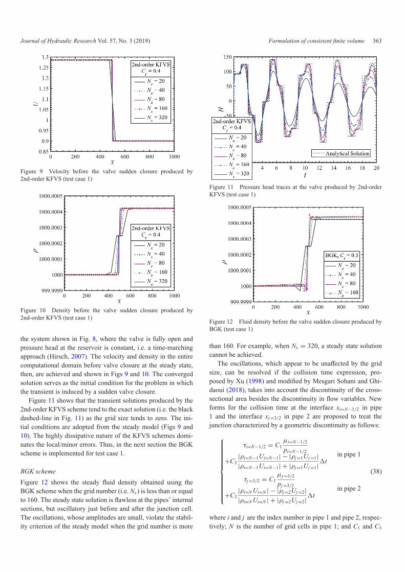
Figure 9 Velocity before the valve sudden closure produced by2nd-order KFVS (test case 1)
Figure 10 Density before the valve sudden closure produced by2nd-order KFVS (test case 1)
the system shown in Fig. 8, where the valve is fully open andpressure head at the reservoir is constant, i.e. a time-marchingapproach (Hirsch, 2007). The velocity and density in the entirecomputational domain before valve closure at the steady state,then, are achieved and shown in Figs 9 and 10. The convergedsolution serves as the initial condition for the problem in whichthe transient is induced by a sudden valve closure.
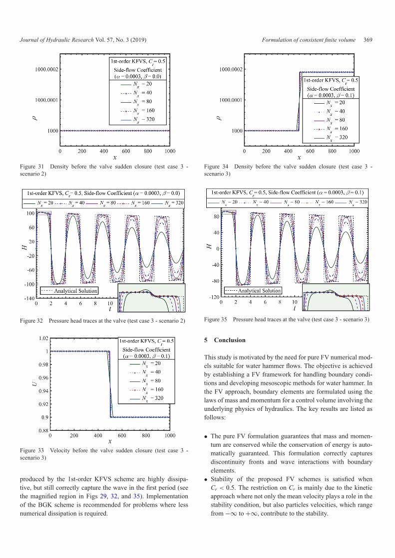
Figure 11 shows that the transient solutions produced by the2nd-order KFVS scheme tend to the exact solution (i.e. the blackdashed-line in Fig. 11) as the grid size tends to zero. The ini-tial conditions are adopted from the steady model (Figs 9 and10). The highly dissipative nature of the KFVS schemes domi-nates the local/minor errors. Thus, in the next section the BGKscheme is implemented for test case 1.
BGK scheme
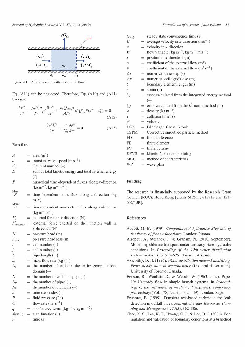
Figure 12 shows the steady fluid density obtained using theBGK scheme when the grid number (i.e. Nx) is less than or equalto 160. The steady state solution is flawless at the pipes’ internalsections, but oscillatory just before and after the junction cell.The oscillations, whose amplitudes are small, violate the stabil-ity criterion of the steady model when the grid number is more
Figure 11 Pressure head traces at the valve produced by 2nd-orderKFVS (test case 1)
Figure 12 Fluid density before the valve sudden closure produced byBGK (test case 1)
than 160. For example, when Nx = 320, a steady state solutioncannot be achieved.
The oscillations, which appear to be unaffected by the gridsize, can be resolved if the collision time expression, pro-posed by Xu (1998) and modified by Mesgari Sohani and Ghi-daoui (2018), takes into account the discontinuity of the cross-sectional area besides the discontinuity in flow variables. Newforms for the collision time at the interface xi=N−1/2 in pipe1 and the interface xj =3/2 in pipe 2 are proposed to treat thejunction characterized by a geometric discontinuity as follows:
⎧⎪⎪⎪⎪⎪⎪⎪⎪⎪⎪⎨⎪⎪⎪⎪⎪⎪⎪⎪⎪⎪⎩
τi=N−1/2 = C1μi=N−1/2
pi=N−1/2
+C3|ρi=N−1Ui=N−1| − |ρj =1Uj =1||ρi=N−1Ui=N−1| + |ρj =1Uj =1|�t
in pipe 1
τj =3/2 = C1μj =3/2
pj =3/2
+C3|ρi=N Ui=N | − |ρj =2Uj =2||ρi=N Ui=N | + |ρj =2Uj =2|�t
in pipe 2
(38)
where i and j are the index number in pipe 1 and pipe 2, respec-tively; N is the number of grid cells in pipe 1; and C1 and C3

364 S. Mesgari Sohani and M.S. Ghidaoui Journal of Hydraulic Research Vol. 57, No. 3 (2019)
Figure 13 Velocity before the valve sudden closure produced by BGKwith the modified collision term (test case 1)
Figure 14 Density before the valve sudden closure produced by BGKwith the modified collision term (test case 1)
are constants and determined from numerical experimentations.The modified numerical terms in Eq. (38) (i.e. the second termsin the right-hand side of Eq. (38)) determine the collision timeby coupling the flow variables of the last cell in pipe 1 and thoseof the first cell of pipe 2. For the computational experimentation,oscillation-free results are achieved when C1 and C3 are set to1.0 and 10.0, respectively. The obtained steady state solutionsproduced by the BGK scheme with the modified collision time(Eq. (38)) are shown in Figs 13 and 14.
Figure 15 presents the pressure head traces at the valve pro-duced by the BGK scheme for Cr = 0.5. In the BGK scheme,the collision time is calculated from Eq. (38) around the junc-tion and the initial conditions are adopted from the achievedsteady state shown in Figs 13 and 14. The results shown inFig. 15 converge to the analytical solution as �x and �t tend tozero. However, slight local discrepancies are observed at t = 8 s,t = 10 s, t = 17 s, and t = 19 s in Fig. 15. As the grid size isreduced, the amplitude of the discrepancies reduces but does notvanish (see the magnified region in Fig. 15). The origin of thediscrepancies is a local energy dissipation (hloss) at steady stateimposed by the junction boundary treatment (Eqs (8) and (10)).To illustrate how the local energy dissipation at the junction is
Figure 15 Pressure head traces at the valve produced by BGK withthe modified collision term (test case 1)
included in the boundary formulation, the mass and momentumconservation laws are formulated at the junction where pipe 1and pipe 2 are connected as follows:
U1A1 = U2A2 (39)
ρA2U22 − ρA1U2
1 = P1A1 + P′(A2 − A1)− P2A2 (40)
where P′ is the pressure acting on the vertical wall of the junc-tion (i.e. A2 − A1). It is found that P1 ∼= P′ for the small radialacceleration at the junction. From Eqs (39) and (40), the energyequation at the junction is derived as follows:
P1
9.81ρ+ U2
1
2 × 9.81= P2
9.81ρ+ U2
2
2 × 9.81+ hloss (41)
where
hloss = U22
2 × 9.81+ U2
1
2 × 9.81− U1U2
9.81(42)
In Eq. (42), hloss is the pressure head loss (i.e. the local energydissipation) at the junction. hloss is physically described by eddymotion formation near the junction. Such a local dissipationmechanism is also observed in the hydraulic jump, as discussedby Abbott (1979).
Comparison of the mesoscopic-based schemes
Figure 16 represents the head traces produced by themesoscopic-based schemes for Nx = 320. In spite of the highlydissipative nature of the KFVS schemes, they reproduce the cor-rect form of the transient waves, particularly during the firstwave cycle. In addition, E/E0 for different schemes is givenin Fig. 17 for Nx = 320, where E is the total energy (i.e. thesum of kinetic and internal energy) in the pipe proposed by Kar-ney (1990). In the pipe, the velocity and, thus, the work at thevalve are zero. In addition, the pressure wave and, thus, the work

Journal of Hydraulic Research Vol. 57, No. 3 (2019) Formulation of consistent finite volume 365
Figure 16 Pressure head traces at the valve produced by the meso-scopic-based schemes for Nx = 320 (test case 1)
Figure 17 Energy head traces for the mesoscopic-based schemeswhen Nx = 320 (test case 1)
at the reservoir are zero. Moreover, the friction and, thus, theenergy dissipation are zero. As result, the total energy is invari-ant with time: E/E0 = 1, where E0 is the total energy beforeany disturbance. Thus, any deviation of E/E0 from 1 is due tonumerical dissipations. ξE , shown in Fig. 17, indicates the errorscalculated from the integral energy equation as follows:
ξE = 1 − EE0
(43)
The numerical errors are measured from the energy equationof Karney (1990) (i.e. ξE) and the L2-norm method (i.e. ξL2 ) asthe functions of the number of grids and are shown in Figs 18and 19, respectively.
For test case 1, the computational time required to reach thesteady state solution denoted tsteady are reported in Table 3. Fromthe results of numerical experimentations, it is observed thatmesoscopic-based schemes require more time steps to reach asteady state as the grid cell size is reduced. For the BGK scheme,the required convergence time is enormously large when Nx =320. The poor convergence of the BGK scheme to steady state,as reported by Xu (1998), is due to time-dependent fluxes of the
Figure 18 ξE versus the number of grids (test case 1)
Figure 19 ξL2 versus the number of grids (test case 1)
BGK scheme. For the steady state calculation Xu (1998) sug-gested that the relaxation process must be simplified in order toyield time independent numerical fluxes. Testing the assertionof Xu (1998) will be left to a future study.
4.2 Test case 2: wave interaction with a junctioncharacterized by a discontinuity in the value of wavespeed
Figure 20 depicts the system configuration for test case 2, whichincludes two pipe segments in series connected to an upstreamreservoir and a downstream valve. The material and thickness ofpipe 1 are different from those of pipe 2, resulting in a change ofwave speed across the junction joining the two pipes. To eval-uate the effect of a discontinuity in wave speed, the flow insidethe pipe is subjected to a severe transient due to sudden closureof the downstream valve. Test case 2 is designed to investi-gate the capability of the mesoscopic-based schemes to simulatetransients when the value of the wave speed changes abruptly.
The relevant geometric and hydraulic parameters for thenumerical test case 2 are provided in Table 4. Wall frictionand local losses at the junction are neglected so any dissipa-tion observed will be purely numerical. In this way, numericaldissipation can be quantified.

366 S. Mesgari Sohani and M.S. Ghidaoui Journal of Hydraulic Research Vol. 57, No. 3 (2019)
Table 3 Converging time tsteady for test case 1
Nx 1st-KFVS scheme (Cr = 0.5) 2nd-KFVS scheme (Cr = 0.4) BGK scheme (Cr = 0.5)
tsteady (s) �t (s) tsteady (s) �t (s) tsteady (s) �t (s)
20 400 0.025 400 0.02 400 0.02540 400 0.0125 400 0.01 400 0.012580 400 0.00625 400 0.005 400 0.00625160 400 0.003125 400 0.0025 800 0.003125320 600 0.0015625 600 0.00125 20,000 0.0015625
Figure 20 The system configuration for test case 2
Table 4 Geometric and hydraulic parameters for test case 2a
Pipe no. L (m) a (ms−1) A (m2)
Pipe 1 500 1000 1Pipe 2 400 800 1
a The discontinuous wave is evoked by a sudden valve closure of thedownstream valve. The initial mass flow rate (i.e. m0) in pipe 1 andpipe 2 is 900 kgs−1 where the initial density is 1000 kgm−3.
Similar to test case 1, both steady and unsteady models arerequired in order to investigate transient behaviours. This testscenario uses the reservoir-pipe-valve system shown in Fig. 20,where the valve is fully opened and pressure head at the reser-voir is constant. In the unsteady models, the same discretetime-dependent model is used such that the converged flowvariables serve as the initial condition and the transient is ini-tiated by a sudden valve closure. The numerical results obtainedfrom the steady model and the unsteady model are discussedseparately in the next section.
The steady model
The converged flow variables for test case 2 produced by the1st-order KFVS are shown in Figs 21 and 22. The state flowvariables obtained from the 2nd-order KFVS and BGK schemesare similar to those variables produced by the 1st-order KFVSscheme.
The proposed compressible models cause a sharp change offluid density across the pipe junction (Fig. 22). To investigatewhy the proposed models impose such a large, unrealistic den-sity in the steady state, the conservation equations of mass andmomentum are applied at the junction, where pipe 1 and pipe 2are connected, as follows:
U1ρ1 = U2ρ2 (44)
Figure 21 Velocity before the valve sudden closure produced by1st-order KFVS (test case 2)
Figure 22 Density before the valve sudden closure produced by1st-order KFVS (test case 2)
ρ2U22 − ρ1U2
1 = P1 − P2 (45)
Starting from the mass and momentum conservation equations(Eqs (44) and (45)), the energy equation associated with the flowinside the pipes is obtained below:
P1
9.81ρ1+ U2
1
2 × 9.81= P2
9.81ρ2+ U2
2
2 × 9.81+�H (46)
where
�H =(
U1
U2− 1
)a2
2
9.81− (U2 − U1)
2
2 × 9.81(47)

Journal of Hydraulic Research Vol. 57, No. 3 (2019) Formulation of consistent finite volume 367
Figure 23 Stress–strain curves for pipe wall and fluid
In Eq. (47), �H is the energy (head) difference between twopipes. The second term in the right hand-side of Eq. (47) is neg-ligible. In addition, the momentum equation (Eq. (45)) impliesU2/U1 ∼= a2
2/a21. Thus, Eq. (47) becomes:
�H ∼= (a2 + a1)(a2 − a1)
9.81(48)
�H is considerably large, and so is the corresponding �E. Thelarge energy difference in two pipes is mainly because the cur-rent mesoscopic-based models solve fluid itself in pipes andexclude any interaction between fluid and pipe wall, so fluid inpipe 1 and pipe 2 stores the total energy. However, in a realisticflow-pipe system, part of the total energy is taken by the fluidand the remainder is taken by the pipe wall. Therefore, for thecase of two pipes in series, with no losses, the energy equationis represented as follows:
Efluid pipe1 + Ewall pipe1 = Efluid pipe2 + Ewall pipe2 (49)
Consider the case in which pipe 1 is more rigid than pipe 2 (i.e.a1 > a2). Hence, for the same deformation, the proportion ofenergy taken by the wall of pipe 1 is larger than that taken bythe wall of pipe 2. Thus, the energy stored in the fluid of pipe2 is larger than that in the fluid of pipe 1. Therefore, the energyequation associated with the fluid itself becomes:
Efluid pipe2 − Efluid pipe1 = �E (50)
where �E is the difference between Ewall pipe1 and Ewall pipe2 andis quantitatively similar to the corresponding �E obtained fromEq. (48). While�E taken by the pipe wall results in a relativelysmall strain in the pipe wall (i.e. εpipe wall), the same proportionof energy taken by fluid induces a large strain (i.e. εfluid). This isillustrated in Fig. 23 where the stress–strain curves correspond-ing to both the pipe wall and fluid are plotted. The hatched areasunder both curves are quantitatively represent �E.
Even though such an extreme partitioning of energy in thesteady state solution is observed in the numerical model atsteady state, the net pressure in the unsteady model gives quitereasonable numerical results. The unsteady results are discussedin the next section.
Figure 24 Pressure head traces at the valve for Nx = 360 (test case 2)
Figure 25 ξL2 versus the number of grid (test case 2)
The unsteady model
Figure 24 show the pressure head traces at the valve producedby the 1st-order KFVS scheme, the 2nd-order KFVS scheme,and the BGK scheme, respectively when Cr = 0.5.
Figure 24 is produced to compare the numerical results pro-duced by the mesoscopic-based schemes when Cr = 0.5 andNx = 320. The relation between the ξL2 and the number of grids,shown in Fig. 25, indicates that the convergence rate of the BGKscheme is significantly larger than that of the KFVS schemes.
4.3 Test case 3: wave interaction with a junctioncharacterized by a flow rate discontinuity
Figure 26 shows a reservoir-pipe-valve configuration for testcase 3. The pipe is connected to an upstream reservoir and adownstream valve. An external flow (i.e. QExt) takes place in themiddle of the pipe. A transient flow inside the pipe is inducedby the sudden closing of the downstream valve. Test case 3 isused to study the capability of the mesoscopic-based scheme tocapture the wave interaction with an external flow. The relevantgeometric and hydraulic parameters for numerical test case 3 aregiven in Table 5.

368 S. Mesgari Sohani and M.S. Ghidaoui Journal of Hydraulic Research Vol. 57, No. 3 (2019)
Figure 26 The system configuration for test case 3
Table 5 Geometric and hydraulic parameters for test case 3a
Pipe no. L (m) a (ms−1) A (m2)
Pipe 1 1000 1000 0.9
a The discontinuous wave is evoked by a sudden valve closure ofthe downstream valve. The initial mass flow rate (i.e. m0) driven bythe reservoir inside pipe 1 is 900 kgs−1 where the initial density is1000 kgm−3.
Figure 27 Velocity before the valve sudden closure (test case 3 -scenario 1)
Similar to the previous test cases, both the steady andunsteady models of compressible fluids are needed. Apart fromreplacing the junction boundary characterized by a change inwave speed by one characterized by a discontinuity in flow rate,the other boundary conditions imposed for test case 3 are sim-ilar to those for test case 2. Numerical experiments using the1st-order KFVS scheme are carried out and presented for testcase 3 in the next section.
1st-order KFVS scheme
Transient properties in a single pipe are affected by the amountof the external flow. Therefore, to investigate how a transientwave interacts with an arbitrary external flow, three scenariosare proposed for the coefficient of the external flow (Eq. (16)) asfollows:
Scenario 1: α = 0.0 m2 and β = 0.1 m3 s−1
Scenario 2: α = 0.0003 m2 and β = 0.0 m3 s−1
Scenario 3: α = 0.0003 m2 and β = 0.1 m3 s−1
Figure 28 Density before the valve sudden closure (test case 3 -scenario 1)
Figure 29 Pressure head traces at the valve (test case 3 - scenario 1)
Figure 30 Velocity before the valve sudden closure (test case 3 -scenario 2)
Figures 27–35 show the converged steady state solutions andtransient solutions corresponding to each scenario. In all scenar-ios the numerical solutions converge to the analytical solutionswhen �x → 0, �t → 0, and �xJ → 0. The numerical results
Journal of Hydraulic Research Vol. 57, No. 3 (2019) Formulation of consistent finite volume 369
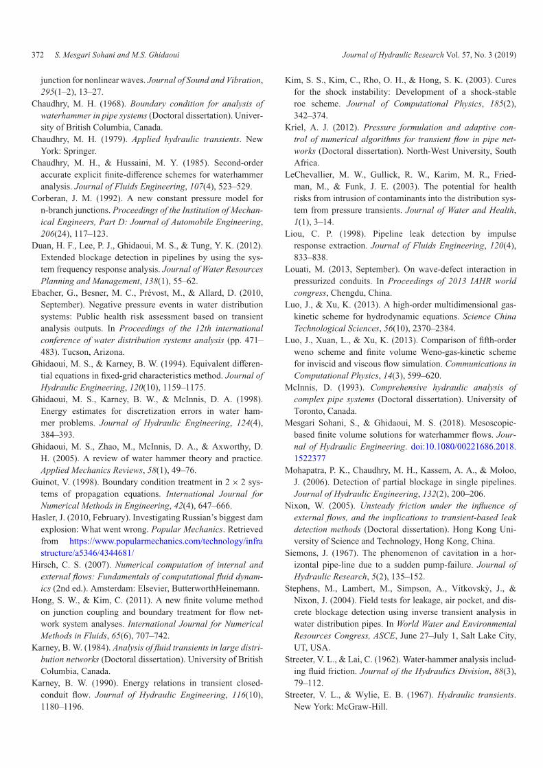
Figure 31 Density before the valve sudden closure (test case 3 -scenario 2)
Figure 32 Pressure head traces at the valve (test case 3 - scenario 2)
Figure 33 Velocity before the valve sudden closure (test case 3 -scenario 3)
produced by the 1st-order KFVS scheme are highly dissipa-tive, but still correctly capture the wave in the first period (seethe magnified region in Figs 29, 32, and 35). Implementationof the BGK scheme is recommended for problems where lessnumerical dissipation is required.
Figure 34 Density before the valve sudden closure (test case 3 -scenario 3)
Figure 35 Pressure head traces at the valve (test case 3 - scenario 3)
5 Conclusion
This study is motivated by the need for pure FV numerical mod-els suitable for water hammer flows. The objective is achievedby establishing a FV framework for handling boundary condi-tions and developing mesoscopic methods for water hammer. Inthe FV approach, boundary elements are formulated using thelaws of mass and momentum for a control volume involving theunderlying physics of hydraulics. The key results are listed asfollows:
• The pure FV formulation guarantees that mass and momen-tum are conserved while the conservation of energy is auto-matically guaranteed. This formulation correctly capturesdiscontinuity fronts and wave interactions with boundaryelements.
• Stability of the proposed FV schemes is satisfied whenCr < 0.5. The restriction on Cr is mainly due to the kineticapproach where not only the mean velocity plays a role in thestability condition, but also particles velocities, which rangefrom −∞ to +∞, contribute to the stability.

370 S. Mesgari Sohani and M.S. Ghidaoui Journal of Hydraulic Research Vol. 57, No. 3 (2019)
• The non-iterative boundary treatment for sudden valve clo-sure, fully open valve, reservoir, and junction boundaryconditions are successfully formulated.
Traditionally, FV solutions are designed with the premisethat there is a set of governing equations that are solved through-out the flow domain together with simple boundary conditions,such as zero velocities normal and tangential to a wall. Suchschemes are not readily applicable to open and closed conduitswhere the boundaries are more complex and often dynamic. Thispaper is a first attempt at showing that it is possible to designa consistent FV scheme for pipe flows by applying the lawsof mass and momentum to a control volume that contains theboundary elements. Future work needs to be carried out to gen-eralize the proposed framework to a wider range of devices anddiscontinuities in closed/open conduit applications.
Appendix. Derivation of one-dimensional equations for atransient flow with an orifice-type external flow
To derive the unsteady flow equations (i.e. mass and momen-tum equations) in a rigid pipe with a external flow, a controlvolume between x = x1 and x = x2, shown in Fig. A1, is con-sidered. The derivation closely follows the derivation of Wanget al. (2002). The pipe is assumed to be horizontal and friction-less with an external flow located in x = xL as shown in Fig. A1,where QExt is the external flow rate (Eq. (16)).
The conservation of mass in the control volume gives:
∂
∂t
∫ x2
x1
(ρA) dx +∫
x1
ρU dA −∫
x2
ρU dA = −ρQExt (A1)
where x is the distance along the pipe; t is the time; ρ is thefluid density; A is the pipe cross-sectional area; U is the averagevelocity in x-direction; and QExt is the external flow rate. Theintegral terms in Eq. (A1) can be simplified as:
∂(ρA)∂t
�x + (ρUA)x2 − (ρUA)x1 = −ρQExt (A2)
where �x is the horizontal distance between x = x1 and x = x2;and the last two terms in the left hand-side of Eq. (A2) are themass fluxes at x = x1 and x = x2. Dividing Eq. (A2) by �x andletting �x approach zero gives:
∂(ρ)
∂t+ ∂(ρU)
∂x+ ρQExtδ(x − xL)
A= 0 (A3)
where δ is the Dirac delta function (Nixon, 2005; Wanget al., 2002) and is defined:
δ(x − xL) ={
∞ if x = xL
0 otherwise, lim
ψ→∞
∫ xL+ψ
xL−ψδ(x − xL) dx = 1
(A4)where ψ is a small distance on the either side of the leak.Similarly, conservation of momentum in the control volume
gives:
∂
∂t
∫ x2
x1
(ρUA) dx +∫
x1
ρU2 dA +∫
x2
ρU2 dA + (PA)x2
− (PA)x1 − ρUQExt = 0 (A5)
where P is pressure. After simplification of the integral terms,Eq. (A5) becomes:
∂(ρUA)∂t
�x + (ρU2A + PA)x2 − (ρU2A + PA)x1 − ρUQExt = 0(A6)
After dividing Eq. (A6) by �x, Eq. (A6) as �x tends to zerogives:
∂(ρU)∂t
+ ∂(ρU2 + P)∂x
− ρUQExtδ(x − xL)
A= 0 (A7)
The external flow rate (Eq. (16)) is:
QExt = sign(HL − H0)α√
2 × 9.81(HL − H0)+ β (A8)
Equations (A3), (A7) and (A8) govern the unsteady flow insidea rigid pipe with an external flow such that the state equationis ∂P/∂ρ = a2, where a is wave speed. To non-dimensionalizeEqs (A3), (A7) and (A8), the following dimensionless quantitiesare used:
P∗ = PP0
, ρ∗ = ρ
ρ0, t∗ = t
L/a, x∗ = x
L,
U∗ = UU0
, Q∗Ext = QExt
QExt0, δ(x∗ − x∗
L) = δ(x − xL)L (A9)
where P0 is the reference pressure; ρ0 is the reference fluiddensity; L is the pipe length; a is the wave speed; QExt0 is thereference external flow rate and U0 is the reference flow rate.Applying the dimensionless quantities (Eqs (A9), Eqs (A3) and(A7) become:
∂P∗
∂t∗+ U0
aU∗ ∂P∗
∂x∗ + ρ0U0aP0
ρ∗ ∂U∗
∂x∗
+ aρ0QExt0
AP0ρ∗Q∗
Extδ(x∗ − x∗
L) = 0 (A10)
∂ρ∗U∗
∂t∗+ U0
a∂ρ∗U∗2
∂x∗ + aU0
∂ρ∗
∂x∗
+ −U0
aQExt0
AU0U∗ρ∗Q∗
Extδ(x∗ − x∗
L) = 0 (A11)
Because U0/a is normally so small in water hammer application,the second term in Eq. (A10) and the second and last terms in
Journal of Hydraulic Research Vol. 57, No. 3 (2019) Formulation of consistent finite volume 371
Ext
L
Figure A1 A pipe section with an external flow
Eq. (A11) can be neglected. Therefore, Eqs (A10) and (A11)become:
∂P∗
∂t∗+ ρ0U0a
P0ρ∗ ∂U∗
∂x∗ + ρ0QExt0 aAP0
ρ∗Q∗Extδ(x
∗ − x∗L) = 0
(A12)
∂ρ∗U∗
∂t∗+ a
U0
∂ρ∗
∂x∗ = 0 (A13)
Notation
A = area (m2)a = transient wave speed (m s−1)Cr = Courant number (–)E = sum of total kinetic energy and total internal energy
(J)F = numerical time-dependent fluxes along x-direction
(kg m−2, kg m−1 s−1)MassF = time-dependent mass flux along x-direction (kg
m−2)MomF = time-dependent momentum flux along x-direction
(kg m−1 s−1)F ′
x = external force in x-direction (N)F ′
Junction = external force exerted on the junction wall inx-direction (N)
H = pressure head (m)hloss = pressure head loss (m)i = cell number (–)j = cell number (–)L = pipe length (m)m = mass flow rate (kg s−1)Nx = the number of cells in the entire computational
domain (–)N = the number of cells in a pipe (–)NP = the number of pipes (–)NE = the number of elements (–)n = time step index (–)P = fluid pressure (Pa)Q = flow rate (m3 s−1)q = sink/source terms (kg s−1, kg m s−2)sign(·) = sign function (–)t = time (s)
tsteady = steady state convergence time (s)U = average velocity in x-direction (m s−1)u = velocity in x-directionW = flow variable (kg m−3, kg m−3 m s−1)x = position in x-direction (m)α = coefficient of the external flow (m2)β = coefficient of the external flow (m3 s−1)�t = numerical time step (s)�x = numerical cell (grid) size (m)δ = boundary element length (m)ε = strain (–)ξE = error calculated from the integrated energy method
(–)ξL2 = error calculated from the L2-norm method (m)ρ = density (kg m−3)τ = collision time (s)–V = volumeBGK = Bhatnagar–Gross–KrookCSPM = Corrective smoothed particle methodFD = finite differenceFE = finite elementFV = finite volumeKFVS = kinetic flux vector splittingMOC = method of characteristicsWP = wave plan
Funding
The research is financially supported by the Research GrantCouncil (RGC), Hong Kong [grants 612511, 612713 and T21-602/15R].
References
Abbott, M. B. (1979). Computational hydraulics-Elements ofthe theory of free surface flows. London: Pitman.
Aisopou, A., Stoianov, I., & Graham, N. (2010, September).Modelling chlorine transport under unsteady-state hydraulicconditions. In Proceeding of the 12th water distributionsystem analysis (pp. 613–625). Tucson, Arizona.
Axworthy, D. H. (1997). Water distribution network modelling:From steady state to waterhammer (Doctoral dissertation).University of Toronto, Canada.
Benson, R., Woollatt, D., & Woods, W. (1963, June). Paper10: Unsteady flow in simple branch systems. In Proceed-ings of the institution of mechanical engineers, conferenceproceedings (Vol. 178, No. 9, pp. 24–49). London: Sage.
Brunone, B. (1999). Transient test-based technique for leakdetection in outfall pipes. Journal of Water Resources Plan-ning and Management, 125(5), 302–306.
Chae, K. S., Lee, K. T., Hwang, C. J., & Lee, D. J. (2006). For-mulation and validation of boundary conditions at a branched
372 S. Mesgari Sohani and M.S. Ghidaoui Journal of Hydraulic Research Vol. 57, No. 3 (2019)
junction for nonlinear waves. Journal of Sound and Vibration,295(1–2), 13–27.
Chaudhry, M. H. (1968). Boundary condition for analysis ofwaterhammer in pipe systems (Doctoral dissertation). Univer-sity of British Columbia, Canada.
Chaudhry, M. H. (1979). Applied hydraulic transients. NewYork: Springer.
Chaudhry, M. H., & Hussaini, M. Y. (1985). Second-orderaccurate explicit finite-difference schemes for waterhammeranalysis. Journal of Fluids Engineering, 107(4), 523–529.
Corberan, J. M. (1992). A new constant pressure model forn-branch junctions. Proceedings of the Institution of Mechan-ical Engineers, Part D: Journal of Automobile Engineering,206(24), 117–123.
Duan, H. F., Lee, P. J., Ghidaoui, M. S., & Tung, Y. K. (2012).Extended blockage detection in pipelines by using the sys-tem frequency response analysis. Journal of Water ResourcesPlanning and Management, 138(1), 55–62.
Ebacher, G., Besner, M. C., Prévost, M., & Allard, D. (2010,September). Negative pressure events in water distributionsystems: Public health risk assessment based on transientanalysis outputs. In Proceedings of the 12th internationalconference of water distribution systems analysis (pp. 471–483). Tucson, Arizona.
Ghidaoui, M. S., & Karney, B. W. (1994). Equivalent differen-tial equations in fixed-grid characteristics method. Journal ofHydraulic Engineering, 120(10), 1159–1175.
Ghidaoui, M. S., Karney, B. W., & McInnis, D. A. (1998).Energy estimates for discretization errors in water ham-mer problems. Journal of Hydraulic Engineering, 124(4),384–393.
Ghidaoui, M. S., Zhao, M., McInnis, D. A., & Axworthy, D.H. (2005). A review of water hammer theory and practice.Applied Mechanics Reviews, 58(1), 49–76.
Guinot, V. (1998). Boundary condition treatment in 2 × 2 sys-tems of propagation equations. International Journal forNumerical Methods in Engineering, 42(4), 647–666.
Hasler, J. (2010, February). Investigating Russian’s biggest damexplosion: What went wrong. Popular Mechanics. Retrievedfrom https://www.popularmechanics.com/technology/infrastructure/a5346/4344681/
Hirsch, C. S. (2007). Numerical computation of internal andexternal flows: Fundamentals of computational fluid dynam-ics (2nd ed.). Amsterdam: Elsevier, ButterworthHeinemann.
Hong, S. W., & Kim, C. (2011). A new finite volume methodon junction coupling and boundary treatment for flow net-work system analyses. International Journal for NumericalMethods in Fluids, 65(6), 707–742.
Karney, B. W. (1984). Analysis of fluid transients in large distri-bution networks (Doctoral dissertation). University of BritishColumbia, Canada.
Karney, B. W. (1990). Energy relations in transient closed-conduit flow. Journal of Hydraulic Engineering, 116(10),1180–1196.
Kim, S. S., Kim, C., Rho, O. H., & Hong, S. K. (2003). Curesfor the shock instability: Development of a shock-stableroe scheme. Journal of Computational Physics, 185(2),342–374.
Kriel, A. J. (2012). Pressure formulation and adaptive con-trol of numerical algorithms for transient flow in pipe net-works (Doctoral dissertation). North-West University, SouthAfrica.
LeChevallier, M. W., Gullick, R. W., Karim, M. R., Fried-man, M., & Funk, J. E. (2003). The potential for healthrisks from intrusion of contaminants into the distribution sys-tem from pressure transients. Journal of Water and Health,1(1), 3–14.
Liou, C. P. (1998). Pipeline leak detection by impulseresponse extraction. Journal of Fluids Engineering, 120(4),833–838.
Louati, M. (2013, September). On wave-defect interaction inpressurized conduits. In Proceedings of 2013 IAHR worldcongress, Chengdu, China.
Luo, J., & Xu, K. (2013). A high-order multidimensional gas-kinetic scheme for hydrodynamic equations. Science ChinaTechnological Sciences, 56(10), 2370–2384.
Luo, J., Xuan, L., & Xu, K. (2013). Comparison of fifth-orderweno scheme and finite volume Weno-gas-kinetic schemefor inviscid and viscous flow simulation. Communications inComputational Physics, 14(3), 599–620.
McInnis, D. (1993). Comprehensive hydraulic analysis ofcomplex pipe systems (Doctoral dissertation). University ofToronto, Canada.
Mesgari Sohani, S., & Ghidaoui, M. S. (2018). Mesoscopic-based finite volume solutions for waterhammer flows. Jour-nal of Hydraulic Engineering. doi:10.1080/00221686.2018.1522377
Mohapatra, P. K., Chaudhry, M. H., Kassem, A. A., & Moloo,J. (2006). Detection of partial blockage in single pipelines.Journal of Hydraulic Engineering, 132(2), 200–206.
Nixon, W. (2005). Unsteady friction under the influence ofexternal flows, and the implications to transient-based leakdetection methods (Doctoral dissertation). Hong Kong Uni-versity of Science and Technology, Hong Kong, China.
Siemons, J. (1967). The phenomenon of cavitation in a hor-izontal pipe-line due to a sudden pump-failure. Journal ofHydraulic Research, 5(2), 135–152.
Stephens, M., Lambert, M., Simpson, A., Vítkovsky, J., &Nixon, J. (2004). Field tests for leakage, air pocket, and dis-crete blockage detection using inverse transient analysis inwater distribution pipes. In World Water and EnvironmentalResources Congress, ASCE, June 27–July 1, Salt Lake City,UT, USA.
Streeter, V. L., & Lai, C. (1962). Water-hammer analysis includ-ing fluid friction. Journal of the Hydraulics Division, 88(3),79–112.
Streeter, V. L., & Wylie, E. B. (1967). Hydraulic transients.New York: McGraw-Hill.

Journal of Hydraulic Research Vol. 57, No. 3 (2019) Formulation of consistent finite volume 373
Streeter, V. L., Wylie, E. B., & Bedford, W. (1998). Fluidmechanics. Boston, MA: WCB/McGraw-Hill.
Thornton, J., Sturm, R., & Kunkel, G. (2008). Water loss control(Vol. 2). New York: McGraw-Hill Professional.
Wang, X.-J., Lambert, M. F., Simpson, A. R., Liggett, J. A., &Vítkovsky, J. P. (2002). Leak detection in pipelines using thedamping of fluid transients. Journal of Hydraulic Engineer-ing, 128(7), 697–711.
Wylie, E. B., Streeter, V. L., & Suo, L. (1993). Fluid transientsin systems (Vol. 1). Englewood Cliffs, NJ: Prentice Hall.
Xu, K. (1998). Gas-kinetic schemes for unsteady compressibleflow simulations. Lecture Series- Van Kareman Institute forFluid Dynamics (VKI), 3, C1–C202.
Zhao, M., & Ghidaoui, M. S. (2004). Godunov-type solutionsfor water hammer flows. Journal of Hydraulic Engineering,130(4), 341–348.