form finding and structural analysis of cables with ... · approval of the thesis: form finding and...

FORM FINDING AND STRUCTURAL ANALYSIS OF CABLES WITH MULTIPLE SUPPORTS

A THESIS SUBMITTED TO THE GRADUATE SCHOOL OF NATURAL AND APPLIED SCIENCES

OF MIDDLE EAST TECHNICAL UNIVERSITY

BY

ABDULLAH DEMĐR

IN PARTIAL FULFILLMENT OF THE REQUIREMENTS FOR

THE DEGREE OF MASTER OF SCIENCE IN

CIVIL ENGINEERING

SEPTEMBER 2011

Approval of the thesis:

FORM FINDING AND STRUCTURAL ANALYSIS OF

CABLES WITH MULTIPLE SUPPORTS

Submitted by ABDULLAH DEMĐR in partially fulfillment of the requirements of the degree of Master of Science in Civil Engineering Department Middle East Technical University by,

Prof. Dr. Canan Özgen _____________________ Dean, Graduate School of Natural and Applied Sciences Prof. Dr. Güney Özcebe _____________________ Head of Department, Civil Engineering Assoc. Prof. Dr. M. Uğur Polat Supervisor, Civil Engineering Dept., METU _____________________ Examining Committee Members: Prof. Dr. Mehmet Utku _____________________ Civil Engineering Dept., METU Assoc. Prof. Dr. M. Uğur Polat _____________________ Civil Engineering Dept., METU Prof. Dr. Suha Oral _____________________ Mechanical Engineering Dept., METU Assoc. Prof. Dr. Afşin Sarıtaş _____________________ Civil Engineering Dept., METU Assist. Prof. Dr. Alp Caner _____________________ Civil Engineering Dept., METU Date: _____________________

iii

I hereby declare that all information in this document has been obtained and presented in accordance with academic rules and ethical conduct. I also declare that, as required by these rules and conduct, I have fully cited and referenced all material and results that are not original to this work.

Name, Last name : Abdullah Demir

Signature :

iv

ABSTRACT

FORM FINDING AND STRUCTURAL ANALYSIS OF

CABLES WITH MULTIPLE SUPPORTS

Demir, Abdullah

M.Sc. in Department of Civil Engineering

Supervisor : Assoc. Prof. Dr. Mustafa Uğur Polat

September 2011 ; 111 pages

Cables are highly nonlinear structural members under transverse loading. This

nonlinearity is mainly due to the close relationship between the final geometry under

transverse loads and the resulting stresses in its equilibrium state rather than the

material properties. In practice, the cables are usually used as isolated single-segment

elements fixed at the ends. Various studies and solution procedures suggested by

researchers are available in the literature for such isolated cables. However, not much

work is available for continuous cables with multiple supports.

In this study, a multi-segment continuous cable is defined as a cable fixed at the ends

and supported by a number of stationary roller supports in between. Total cable

length is assumed constant and the intermediate supports are assumed to be

frictionless. Therefore, the critical issue is to find the distribution of the cable length

among its segments in the final equilibrium state. Since the solution of single-

segment cables is available the additional condition to be satisfied for multi-segment

continuous cables with multiple supports is to have stress continuity at intermediate

support locations where successive cable segments meet. A predictive/corrective

iteration procedure is proposed for this purpose. The solution starts with an initially

assumed distribution of total cable length among the segments and each segment is

analyzed as an independent isolated single-segment cable. In general, the stress

v

continuity between the cable segments will not be satisfied unless the assumed

distribution of cable length is the correct distribution corresponding to final

equilibrium state. In the subsequent iterations the segment lengths are readjusted to

eliminate the unbalanced tensions at segment junctions. The iterations are continued

until the stress continuity is satisfied at all junctions. Two alternative approaches are

proposed for the segment length adjustments: Direct stiffness method and tension

distribution method. Both techniques have been implemented in a software program

for the analysis of multi-segment continuous cables and some sample problems are

analyzed for verification. The results are satisfactory and compares well with those

obtained by the commercial finite element program ANSYS.

Keywords: Single-segment cable, multi-segment continuous cable, continuous cable

with multiple supports, tension distribution for continuous cables, Newton-Raphson

iterations

vi

ÖZ

ÇOK MESNETLĐ KABLOLARIN

YAPISAL ANALĐZĐ VE ŞEKĐL TAYĐNĐ

Demir, Abdullah

Yüksek Lisans, Đnşaat Mühendisliği Bölümü

Tez Yöneticisi : Doç. Dr. Mustafa Uğur Polat

Eylül 2011 ; 111 Sayfa

Kablolar yanal yük altındaki davranışı yüksek derecede doğrusal olmayan yapı

elemanlarıdır. Bu durum kabloların malzeme özelliklerinden çok uygulanan yükler

altındaki denge koşulları ile son denge konumundaki geometrisi arasındaki direkt

ilişkiden kaynaklanmaktadır. Uygulamada kablolar genellikle uç noktalarından

sabitlenmiş tek bir eleman olarak kullanılmakta ve bu şekilde analiz edilmektedir.

Literatürde böyle iki ucundan mesnetli tek parça kabloların analizi için birçok

çalışma ve çözüm önerileri mevcuttur. Ancak çok mesnetli sürekli kablolar için

fazlaca bir çalışma bulunmamaktadır.

Bu çalışmada her iki ucundan mesnetlenmiş ve bu mesnetler arasına yerleştirilmiş

sabit makaralı mesnetler ile desteklenmiş çok açıklıklı ve çok mesnetli sürekli

kabloların analizi için bir çözüm yöntemi geliştirilmiştir. Kablo sisteminin toplam

boyunun sabit, ara mesnetlerin ise sürtünmesiz makaralar şeklinde olduğu kabul

edilmektedir. Uç noktalarından mesnetlenmiş ve sabit boydaki kablolar için çözüm

yöntemi bilindiğinden sürekli kablolar için çözülmesi gereken problem, sistemin son

denge konumunda, toplam kablo boyunun açıklıklar arasındaki dağılımının

belirlenmesidir. Bunun için sürekli kablo sisteminde tek açıklıklı izole kablo

çözümüne ilave olarak sağlanması gereken temel koşul ara mesnet noktalarındaki

kablo gerilmelerinin sürekliliğidir. Önerilen iteratif çözüm yönteminde analize kablo

vii

toplam boyunun açıklıklar arasına makul bir dağılımı ile başlanmakta ve herbir

açıklıktaki kablo izole tekil bir kablo olarak çözülmektedir. Daha sonra kablo

boyunun açıklıklar arasındaki dağılımı ara mesnet noktalarında ardaşık kablo

bölümleri arasında oluşan gerilme farkını sıfırlayacak şekilde yeniden belirlenmekte

ve iterasyonlara sistem denge konumuna ulaşana kadar devam edilmektedir. Bu

amaçla iki farklı yaklaşım önerilmektedir: Direkt rijitlik yöntemi ve gerilme dağıtma

yöntemi. Çok mesnetli sürekli kabloların analiz amacı ile her iki yöntemi de kullanan

bir yazılım geliştirilmiş ve değişik yapıdaki örnek kablo sistemler çözümlenmiştir.

Elde edilen sonuçlar tatmin edici olup ticari bir sonlu elemanlar yazılımı olan

ANSYS programı ile elde edilen sonuçlar ile uyum içinde olduğu görülmektedir.

Anahtar Kelimeler: Tek açıklıklı kablo, çok açıklıklı sürekli kablo, çok mesnetli

sürekli kablo, sürekli kablolar için gerilme dağıtma yöntemi, Newton-Raphson

iterasyonu

viii

To My Family

ix

ACKNOWLEDGEMENTS

The author wishes to express his appreciation to Assoc. Prof. Dr. Mustafa Uğur Polat

for his supervision and encouragement.

Thanks to my family DEMĐR; KERĐM, AYŞE, ÖZLEM, HAVVA NUR

x

TABLE OF CONTENTS

ABSTRACT ................................................................................................................ iv

ÖZ ............................................................................................................................... vi

ACKNOWLEDGEMENTS ........................................................................................ ix

TABLE OF CONTENTS ............................................................................................. x

LIST OF TABLES .................................................................................................... xiii

LIST OF FIGURES .................................................................................................. xiv

LIST OF SYMBOLS ................................................................................................ xvi

CHAPTERS ................................................................................................................. 1

1. INTRODUCTION ................................................................................................ 1

1.1 General .......................................................................................................... 1

1.2 Purpose .......................................................................................................... 3

1.3 Previous Studies ............................................................................................ 4

2. SINGLE-SEGMENT CABLE ............................................................................ 13

2.1 General ........................................................................................................ 13

2.2 Cable Equilibrium Equations ...................................................................... 13

2.3 Stiffness Matrix ........................................................................................... 15

2.4 Newton-Raphson Method ............................................................................ 20

3. MULTI-SEGMENT CONTINUOUS CABLE .................................................. 22

3.1 General ........................................................................................................ 22

3.2 Direct stiffness approach ............................................................................. 23

3.3 Relaxation (tension distribution) method .................................................... 26

3.4 Newton-Raphson iterations ......................................................................... 27

3.5 Comparison of Direct Stiffness and Relaxation Approaches. ..................... 30

xi

4. VERIFICATION FOR SINGLE-SEGMENT CABLES .................................... 34

4.1 General ........................................................................................................ 34

4.2 Description of the Problem .......................................................................... 34

4.3 Solution by CABPOS .................................................................................. 35

4.4 Solution by ANSYS .................................................................................... 39

4.5 Comparison of results .................................................................................. 41

5. VERIFICATION FOR MULTI-SEGMENT CONTINUOUS CABLES .......... 44

5.1 General ........................................................................................................ 44

5.2 Description of Problem ............................................................................... 44

5.3 Solution of CABPOS ................................................................................... 46

5.4 Solution of ANSYS ..................................................................................... 47

5.5 Comparison ................................................................................................. 48

6. COMPUTER PROGRAM: CABPOS (CABLE POSITIONING) ..................... 54

6.1 General ........................................................................................................ 54

6.2 Procedure ..................................................................................................... 54

6.3 Main Program .............................................................................................. 55

6.4 Subroutines .................................................................................................. 57

6.4.1 MSPFTC .............................................................................................. 57

6.4.2 MSPFSC ............................................................................................... 58

6.4.3 INPUT1 ................................................................................................ 59

6.4.4 INPUT2 ................................................................................................ 60

6.4.5 COTLOES ............................................................................................ 60

6.4.6 COSCLOES ......................................................................................... 60

6.4.7 DOS ...................................................................................................... 60

6.4.8 ALAI .................................................................................................... 61

6.4.9 AIOES .................................................................................................. 61

xii

6.4.10 COOS ................................................................................................... 61

6.4.11 GIFTFP ................................................................................................ 62

6.4.12 FEC ...................................................................................................... 62

6.4.13 FMEC ................................................................................................... 62

6.4.14 MATINV .............................................................................................. 63

6.4.15 MATMULT ......................................................................................... 63

6.4.16 OUTPUT1 ............................................................................................ 63

6.4.17 MODULUS .......................................................................................... 64

7. SUMMARY, CONCLUSIONS AND RECOMMENDATIONS ...................... 65

7.1 Summary ..................................................................................................... 65

7.2 Conclusions ................................................................................................. 66

7.3 Recommendations for future studies ........................................................... 67

REFERENCES ........................................................................................................... 69

APPENDICES ........................................................................................................... 72

A. CODE OF CABPOS ............................................................................................. 72

B. CODE OF ANSYS MODEL OF SINGLE-SEGMENT CABLE ....................... 104

C. CODE OF ANSYS MODEL OF MULTI-SEGMENT CONTINUOUS CABLE

.................................................................................................................................. 107

xiii

LIST OF TABLES

TABLES

Table 4.1 Support locations ....................................................................................... 35

Table 4.2 Data for cable A-B3 solved with 50 elements. .......................................... 36

Table 4.3 Data for cable A-B3 solved with 100 elements. ........................................ 36



Table 4.6 Data for cable A-B3 solved with 1000 elements. ...................................... 37

Table 4.7 Data for cable A-B3 solved with 10000 elements. .................................... 37

Table 4.8 Support reactions for A-B3 given by CABPOS......................................... 37

Table 4.9 Support reactions for cable A-B3 given by ANSYS.................................. 39

Table 4.10 Reaction results for different configurations. .......................................... 41

Table 4.11 Error of percentages for single-segment cable solutions. ........................ 42

Table 5.1 Coordinates of supports. ............................................................................ 46

Table 5.2 Support reactions of cable F1-F2c given by CABPOS. ............................. 46

Table 5.3 Support reactions of cable F1-F2c given by ANSYS. .............................. 47

Table 5.4 Support reactions for cable F1-F2a. ........................................................... 49

Table 5.5 Support reactions for cable F1-F2b. ........................................................... 49

Table 5.6 Support reactions for cable F1-F2c. ........................................................... 49

Table 5.7 Error of percentages for single-segment cable solution. ............................ 50

xiv

LIST OF FIGURES

FIGURES

Figure 1.1 Pre-stressing by draping the tendons. ......................................................... 2

Figure 1.2 Single-segment cable profile. ..................................................................... 3

Figure 1.3 Multi-segment continuous cable profile. .................................................... 4

Figure 1.4 Cross-section and layout of 7 wire strands ................................................. 4

Figure 1.5 Some types of strands ................................................................................. 5

Figure 1.6 Typical stress-strain relationship of cable .................................................. 6

Figure 1.7 Illustration of cable logging system by Charland J.W.[15] ........................ 9

Figure 1.8 Whole view of the bridge [17] .................................................................. 10

Figure 1.9 View of the saddle [17] ............................................................................ 11

Figure 1.10 Post-tensioned truss bridge [18] ............................................................. 11

Figure 2.1 Configuration of single-segment cable in space. ...................................... 14

Figure 2.2 Reactions on cable .................................................................................... 17

Figure 2.3 Newton Raphson Method in schematic form for single segment cable. .. 21

Figure 3.1 Configuration of multi-segment continuous cable. .................................. 23

Figure 3.2 Reactions (cable tensions) at support i. .................................................... 24

Figure 3.3 Newton Raphson method in schematic form for multi segment continuous

cable. .......................................................................................................................... 29

Figure 3.4 Typical slackness curve of a cable............................................................ 31

Figure 4.1 Reactions at first support given by CABPOS. .......................................... 38

Figure 4.2 Reactions at second support given by CABPOS. ..................................... 38

Figure 4.3 Reactions at first support given by ANSYS. ............................................ 40

Figure 4.4 Reactions at second support given by ANSYS. ....................................... 40

xv

Figure 4.5 Profile of cable A-B3 ................................................................................ 43

Figure 5.1 Sum of support reactions for cable F1-F2c given by CABPOS. .............. 47

Figure 5.2 Sum of support reactions for cable F1-F2c given by ANSYS. ................ 48

Figure 5.3 Profile of cable F1-F2a ............................................................................. 51

Figure 5.4 Profile of cable F1-F2b ............................................................................. 52

Figure 5.5 Profile of cable F1-F2c ............................................................................. 53

xvi

LIST OF SYMBOLS

UL : Unstressed length of cable

SL : Stressed length of cable

AP�

: Position vector of point A

BP�

: Position vector of point B

ul : Unstressed arc length form point A to M

sl : Stressed arc length from point A to M

ˆ( )ulτ : Unit tangent at point M

( )uR l�

: Reaction vector at point M

( )uT l : Reaction at point M

ul∆ : Elongation of the element at point M

( )ulε : Strain of the element at point M

[ ]S : Stiffness matrix

( )ext uF l�

: Total force applied to cable form point A to M

W�

: Distributed load on cable including self weight

E : Modulus of elasticity of cable material

A : Cross-sectional area of cable

υ : Cable constitutive constant

i , j , k : Unit vectors along global coordinate directions X, Y, Z respectively

xvii

[ ]F : Flexibility matrix

[ ]iM�

: Misclose vector

ERR : Target error or precision

[ ]iE : Error at ith iteration

( )u il , ( )s il : Unstressed and stressed length of cable on ith segment

( )iR∆�

: Reaction difference of cable on ith roller support

( )F iR�

: Reaction vector for the first node of the ith segment

( )L iR�

: Reaction vector for the last node of the ith segment

( )iT∆ : Tension difference of cable on ith roller support

( )segment

U iL∆ : Length adjustment applied on ith segment

( )U iL∆ : Length adjustment applied on ith roller support

( )iTδ : Change in unbalanced tension on ith roller support

( )U jLδ : Unstressed length adjustment on jth roller support

[ ]K : Stiffness matrix of multi segment continuous cable

f : Flexibility coefficient

[ ]( )m

u il : Unstressed length of cable on ith segment for mth iteration

1

CHAPTERS

CHAPTER 1

1. INTRODUCTION

1.1 General

Cables, having negligible shear, flexural and torsional rigidities and zero-buckling

load, are invaluable members for structural engineering. They are used in many

structures like guyed towers, cable-stayed bridges, marine vehicles, offshore

structures, cable roofs, transmission lines, pre-stressing applications and tensegrity

works. Mostly, cables are used for large span distances and/or pre-stressing works.

Nonlinearity is a problem for almost all structural elements. In basic, these

nonlinearities occur due to geometrical and material properties of the member. Both

of them are valid for almost all structures. If the member is adequately stiff in lateral

direction, the geometrical nonlinearity could be ignored due to small P-∆ effect.

However, cable is a structural element which has a very small stiffness in lateral

direction because of its tangential geometry. Steel is used as a material for

fabrication of cable. Therefore, cable has the nonlinearity of steel material. Besides,

tangential geometry of the cable gives the cable element another nonlinearity due to

squeeze which could not be classified as purely geometrical or material nonlinearity.

Thus, cable is a nonlinear structural element due to its geometry and material

properties. In this study, modulus of elasticity of the cable material is taken constant.

Only geometric nonlinearity is taken into account.

In structures, both in designing stage and application stage, cables are used as

supported between the two end points. According to this design, cables have a fixed

unstretched length between those supports. The lengthening is only due to stresses

applied on it. However, if cables are designed monolithically and supported by a

number of roller supports, there will be a change in unstretched length of cable for

2

each segment due to loads applied on it. This behavior of cable adds another

nonlinearity to the problem.

In practice, cables are designed as a single-segment and assumed to be linear

structural members. For example, a type of pre-stressing work, shown in Figure 1.1,

is a completely single-segment multi-support cable problem. A monolithic tendon

placed between two end points and supported by a number of roller supports along

its span is a truly nonlinear problem. However, the cable is usually assumed as a

linear member to ease the calculations for this pre-stressing work. Although, the

weight of the cable is negligible for small-scale problems like this example, the cable

cannot be classified as a linear structural member for large scale problems.

Figure 1.1 Pre-stressing by draping the tendons.

In brief, depending on the way they are used in structures, the cable behavior under

transverse loading is a nonlinear problem. In many situations, they are supported not

only at their end points but also at some points along their spans. This, in turn,

further increases the level of nonlinearity due to presence of contact problem.

However, in practice, they are usually treated as single-segment systems and

assumed as linear structural members supported at their end points. This research

gives a different point of view to the analysis of cables supported along their spans.

3

1.2 Purpose

Extensive research has been made under the constraint that loads are applied to some

predefined points on the cable or successive cables are designed separately. This

design logic restricts engineers to design more integrated systems. Because there

could be a number of cable elements in a structure and these cables are designed as

single-segment. All cable elements should be designed and lengths of them should be

determined individually. Besides that restriction of engineer aspect, there are many

structures designed as single-segment cable systems although being multi-segment

continuous cable systems. As an example, draglifts are systems having multi-

segments cable. Instead of the constraint of single-segment cable systems, research

was made to see the behavior of cables placed on roller supports. This approach will

give engineers a wide aspect for designs and research. Also it makes convenient

designs possible. Previous studies and objective study are illustrated in Figure 1.2

and Figure 1.3, respectively.

Figure 1.2 Single-segment cable profile.

4

Figure 1.3 Multi-segment continuous cable profile.

1.3 Previous Studies

Being a useful member for structural systems, make cables more attractive for

researchers. Despite being an important material, it is hard to analyze the cables

because cables are highly nonlinear structural components. These nonlinearities are

due to its material characteristic and behavior under applied loads. Although these

are denoted in different ways, they could not be distinguished. Also, this association

makes the problem more complex. Besides, having many types make cable analysis

harder. Convoluted geometry and some types of cables are shown in Figure 1.4 and

Figure 1.5. These complicated characteristics of cables have been studies of

researchers for a half century. Studies, which have been carried out previously, are

processed into that order; material characteristics of cable, equivalent modulus

approach, finite element approach, single-segment and multi-segment studies.

Figure 1.4 Cross-section and layout of 7 wire strands

5

Figure 1.5 Some types of strands

Stress - strain relationship of cables are hard to determine. Its response under some

stresses shows discrepancy between under low stresses and high stresses. Cables

show relaxation under stresses due to its tangential geometry. If a strain controlled

test is made for cables, it will be seen that relationship with stress is not linear and

the stress - strain graph shows typical inclinations for different types of cables. These

inclinations are illustrated in Figure 1.6. Analyses on stress-strain relationship of

cables were made by several authors. The earlier study was made by Costello [1],

then by Kumar and Cochran [2]. They tried some theoretical approaches related with

cables’ tangential geometry and found some formulas modeling the behavior of

cables. These formulas were compared with stress – strain analysis and accuracy of

them were determined.

6

Figure 1.6 Typical stress-strain relationship of cable

Behavior under applied loads and self weight is another nonlinearity of cable

analysis. Although there were studies made before 1950s, there was no tangible

research for cables and their nonlinear behavior. They assumed linear behavior for

cable. Some researchers tried to make cable analysis after 1950s, nevertheless studies

had not been solved the nonlinear behavior of cables, precisely, until 1980s.

Between 1950s and 1980s, researchers only made some assumptions to minimize the

nonlinear behavior. Researchers performed catenary cable analysis by some

approaches. Equivalent modulus of elasticity is an approach for reaching the catenary

behavior of the cables before computers. This approach was first discussed by F.

Dischinger [3]. Positioning the catenary cable’s shape as parabola instead of its real

shape and neglecting the cable weight are assumptions made in equivalent modulus

of elasticity approach. Equivalent secant modulus of elasticity is another approach,

formulated by Ernst [4]. Hajdin et al. [5] redefined the cables’ equivalent modulus in

1998.

7

Dischinger’s formula [3];

2

2

11

12z

EAEA

g lEAT

T

= +

(1.1)

Hajdin, Michaltsos and Konstantakopoulos [5] derivation result;

( )

( )

2

22

2

31

24

3 3

xz

x x

EAEA

T T g lEA g l

g l g lTT T T

= + − +

− + +

(1.2)

Computer, being a milestone for structural engineering in 1980s, makes some

calculations possible, easy and accurate. This is valid for cable analysis. Computer

makes nonlinear analysis easy and possible. Finite element modeling was used for

nonlinear analysis after the invention of computer.

Finite element method is a model, originally introduced by Turner et al. [6]. FEA is a

numerical technique for approximate solutions of complex problems. These

complexities were called as “real world” problems by Madenci et al. [7]. Some

material, shape and boundary condition properties of problem cause complexities.

All complexities or nonlinearities are valid for cable problem.

The basis of FEA is decomposition of system to find out the solution of the total

system. Each decomposed member of system is called as finite element. Although

Turner et al. [6] established the element matrix assembly; the “finite element” term

was first used by Clough [8]. Idea of FEA does not change; nevertheless there are

lots of finite element types and solution types for problems. The solution will be

approximate, changing with solution techniques e.g. finite element length and shape

function. However, the finite element solutions will approach to the correct result

with the mesh refinement.

The first realistic single-segment cable solution was made by Michalos and Brinstiel

[9]. Skop and O’Hara [10,11] made similar analysis. Approach of this study is a

finite element analysis having trial and error procedure. Procedure of the study is:

8

Cable having supports at both ends is an indeterminate structure, so system is

assumed as one end supported cable to make system statically determinate. Then,

cable layout is formed by finite element analysis procedures. First support’s reactions

are changed by some iterative procedures till cable’s other cusp ends on second

support.

The iterative procedure used by Skop and O’Hara [10,11] is called Method of

Imaginary Reactions. Some research were made on this iterative procedure

technique. Newton Raphson Method was introduced by Polat M.U. in his master

thesis [12] by the supervision of Yılmaz Ç.. Method of Imaginary Reactions and

Newton Raphson Method has same technique in positioning of cable, they differ in

iteration phase. Newton Raphson Method is used in this thesis to decreases the

number of iterations.

Various computer programs have been developed for analysis of cable till now.

Peyrot and Goulois developed one of them [13]. Also, Fleming J.F. [14] coded a

program for nonlinear static analysis of cable-stayed bridge structures which includes

cable analysis. Almost all of them were written by finite element modeling. Also,

CABPOS is finite element modeling computer program for cable analysis developed

within this theses. Except that affinity, CABPOS solves multi-segment continuous

cable systems, while others deal with single-segment cable solutions.

Multi-segment continuous cables are used in daily life. Cable lift, Barriers for

highways, ski tows and teleskis are systems work with cables having multi-segments.

These systems were analyzed by the logic of single-segment cable analysis. Charland

J.W. et all deal with multi-segment continuous cable problems [15] by breaking

cable into segments. They dealed with wood logging systems as seen in Figure 1.7.

There are two supports and a roller support. Charland J.W. called end supports as

Skyline anchor point and roller support as Intermediate support. They coped with this

cable problem by some assumptions. These assumptions are;

1- Cables are assumed to be massless and inextensible.

2- Friction is ignored in the formulation.

3- Tension in each cable is considered to be constant along the cable.

9

4- Intermediate support is a support which does not make any interaction

between two successive supports.

5- Length of cable at segments does not change.

Figure 1.7 Illustration of cable logging system by Charland J.W.[15]

Briefly, Charland J.W. [15] defined a multi-segment continuous cable problem in

1994; however solution of the system is not achieved correctly. The assumptions

made by Charland J.W. simplify the system and made it single-segment cable.

Aufaure M. [16] also defines a multi-segment continuous cable problem. Researcher

dealed with an electricity cable problem having three supports. In this study, a cable

element having three nodes N1, N2, N3 is defined. N1 and N2 are fixed nodes. N3 is

the node which coincides with roller support. This coincidence is found by the

continuity of the tension in the cable. Aufaure M. also made some assumptions. The

most important assumption is: Node N3 must remain between N2 and N1. If not,

convergence does not been reached and new length for an element must be selected.

So, this solution depends on cable element length. Therefore, longer elements will be

10

needed for slack cable problems. Another handicap of the solution is that; this

solution technique is valid for two segment cable systems.

Kwang Sup Chung et all [17] studied on a cable-stayed bridge which has multi-

segment continuous cable system. In their study, they worked on a bridge having

cable with a roller support. This bridge is a cable-stayed bridge having saddle

anchorage, which can be called roller support, in Austria. They used finite element

model for the solution of cable system. They consider the sliding effect on roller

support. Two type of sliding effect is defined by the authors. These are roller sliding

without friction and frictional sliding. Finally, they define a new problem faced on

cable-stayed bridges and solve it. This problem is a nonlinearity of usage of multi-

segment continuous cables on structures. However this solution was also a single-

segment cable solution. They did not deal with the interchange of the cable on the

roller support. Their solution is for friction problem.

The photos of that bridge taken by the author of that study are shown in Figure 1.8

and Figure 1.9. This type of roller supports could be seen on lots of structures mostly

in bridges. For instance, pylons of suspension bridges commonly consist a roller

support. However the effect of roller support does not considered also for those

examples.

Figure 1.8 Whole view of the bridge [17]

11

Figure 1.9 View of the saddle [17]

Kyoung-Bong H. and Sun-Kyun P. [18] defined another multi-segment continuous

cable system. They tried to increase the load-carrying capacity of truss system. They

applied a multi-segment continuous cable system to truss system with the logic of

post-tensioning. A monolithic cable was used for those systems, because it was

applied to an existing structural system. Thus, post-tensioning should be applied by

one jacking operation. They made a parametric study on this system. Many types of

cable configurations were given in the study. One example of those is in Figure 1.10.

However, cable is assumed as a linear element and interchange on roller supports is

not considered.

Figure 1.10 Post-tensioned truss bridge [18]

12

Cable has two segments and/or the structural system is symmetric or cable is

assumed as linear element in almost all structural systems mentioned above.

Although there are various types of solutions and techniques for cable analysis, these

could only give a solution for single-segment cable or partially for multi-segment

continuous cable.

13

CHAPTER 2

2. SINGLE-SEGMENT CABLE

2.1 General

Cables are highly nonlinear in their response under applied transverse loading. The

nonlinearity is mainly due to interaction between its deformed geometry and the

resulting stresses in its final equilibrium state. Early researchers have tried to analyse

cables by adjusting the mechanical properties after some simplifying assumptions

and completely ignoring the geometric component of nonlinearity. However, the

resulting Equivalent Modulus Approach was, naturally, far from yielding satisfactory

results. Correct solutions were obtained by the Method of Imaginary Reactions [10]

and nonlinear finite element analysis using Newton-Raphson iterations. These

analysis techniques are the extension of the Theory of Consistent Deformations.

Although they give approximate solutions, these techniques use no simplifying

assumption and result in the final correct equilibrium state of the cable. Newton-

Raphson method is used in this study. Formulas related to this technique are briefly

explained below.

2.2 Cable Equilibrium Equations

A cable, having total unstressed length UL and stressed length SL , is supported

between points A and B. The view of the cable in space is shown in Figure 2.1.

As illustrated in Figure 2.1, AP�

and BP�

are the position vectors of cable supports. Let

M be any point on the cable defined by the following parameters;

ul ; unstressed arc length form point A to M .

sl ; stressed arc length from point A to M .

14

BP�

AP�

( )uP l�

( ) ( )u uP l dP l+� �

udl

ul

A B

M

X

Y

Z

Figure 2.1 Configuration of single-segment cable in space.

The unit tangent along the cable, ˆ( )ulτ , can be defined as;

( )ˆ( ) u

u

s

dP ll

dlτ =

�

(2.1a)

or

ˆ( ) ( )u u sdP l l dlτ= −�

(2.1b)

The unknowns in Eq. 2.1b are; ˆ( )ulτ and the differential stressed arc length of the

cable sdl .

The unit tangent along the cable can also be defined as

( )ˆ( )

( )u

u

u

R ll

T lτ =

�

(2.2)

where ( )uR l�

is reaction vector at ul , T(lu) is tension at ul and udl is the original

differential length of the cable.

So, the elongation of the differential element is

15

u s ul dl dl∆ = − (2.3)

The strain of this element is the elongation divided by the original length.

( ) s uu

u

dl dll

dlε

−= (2.4)

From Eq. 2.4 the stressed length of the element can be written as

[ ]1 ( )s u udl l dlε= + (2.5)

Substituting Eq. 2.5 into Eq. 2.1b

[ ]ˆ( ) ( ) 1 ( )u u u udP l l l dlτ ε= − +�

(2.6a)

[ ]( )ˆ( ) 1 ( )u

u u

u

dP ll l

dlτ ε= − +

�

(2.6b)

Finally, writing Eq. 2.6b in integral form

[ ]0

( )( ) (0) 1 ( )

( )

ul

u u

R xP l P l dx

T xε= − +∫

��

(2.7a)

Since (0) AP P=� �

,

[ ]0

( )( ) 1 ( )

( )

ul

u A u

R xP l P l dx

T xε= − +∫

��

(2.7b)

Consequently, AR�

, which is equal to 0( )R l�

, is the only unknown in this equation and

it can be regarded as the initial condition of the problem.

2.3 Stiffness Matrix

If a virtual displacement, BP∆�

, is given to support B, there will be a change in the

reactions at the other support, AR∆�

. The relation between these parameters are

explained by the stiffness matrix, [ ]S .

16

[ ]A BR S P∆ = ∆� �

(2.8)

The stiffness matrix is determined by using the variational approach as follows:

From variation of Eq. 2.7b, BP∆�

is determined.

[ ]0

( )1 ( )

( )

UL

uB u u

u

R lP l dl

T lε

∆ = − ∆ +

∫

��

0

1 ( ) 1 ( )( ) ( )

( ) ( )

UL

u uu u u

u u

l lR l R l dl

T l T l

ε ε + += − ∆ + ∆

∫

� � (2.9)

Unknowns are ( )uT l , ( )uR l∆�

and 1 ( )

( )u

u

l

T l

ε+∆ in Eq. 2.9.

[ ] [ ]2

1 ( ) ( ) 1 ( ) ( )1 ( )

( ) ( )u u u uu

u u

l T l l T ll

T l T l

ε εε ∆ + − + ∆+∆ =

[ ]2

( ) ( ) 1 ( ) ( )

( )u u u u

u

l T l l T l

T l

ε ε∆ − + ∆= (2.10)

Thus, unknowns are ( )uT l , ( )uT l∆ , ( )uR l∆�

, ( )ulε∆ in Eq. 2.9.

Tension in cable is

1/ 2

( ) ( ) ( )u u u

T l R l R l = � �i (2.11)

In variational form, ( )uT l∆

1/ 2

( ) ( ) ( )1( )

2 ( ) ( )

u u u

u

u u

R l R l R lT l

R l R l

∆ + ∆ ∆ =

� � �i� �i

(2.12)

Or

( ) ( )( )

( )u u

u

u

R l R lT l

T l

∆∆ =

� �i

(2.13)

17

A

M M

AR�

( )uR l−�

( )uR l�

W�

Figure 2.2 Reactions on cable

Many external forces e.g. wind force, could be applied to the cable. If no external

load is applied, there will be only self-weight of the cable.

( )ext u uF l Wl=� �

(2.14)

From the free body diagram of cable element shown in Figure 2.2, reaction at point

M is;

( ) ( )u A ext uR l R F l= +� � �

(2.15a)

For the whole cable

( ) ( )U A ext UR L R F L= +� � �

(2.15b)

( )B UR R L=� �

(2.16)

Substituting Eq. 2.16 into Eq. 2.15b

( )B A ext uR R F L= +� � �

(2.17)

From variation of Eq. 2.17

( )u A BR l R R∆ = ∆ = ∆� � �

(2.18)

18

The strain can also be expressed by the stress-strain relationship as

( )( ) uu

T ll

EAε υ= (2.19)

( )uT l is the tension at M and E , A and υ are material properties of cable.

The variational form of strain, ( )ulε∆ , from Eq. 2.4

1( ) ( )

( ) u uu

T l T ll

EA EA

υ

ε υ−∆ ∆ =

(2.20a)

2

( ) ( )( )

( )u u

u

u

R l R ll

T lυε

∆=

� �i

(2.20b)

So, substituting Eq. 2.11 Eq. 2.13 and Eq. 2.20b into Eq. 2.10

[ ]2

2

( ) ( ) ( ) ( )( ) ( ) 1 ( )

1 ( ) ( ) ( )

( ) ( )

u u u uu u u

u u u

u u

R l R l R l R ll T l l

l T l T l

T l T l

υε εε

∆ ∆− +

+∆ =

� � � �i i

( )

3

1 1 ( )( ) ( )

( )u

u u

u

lR l R l

T l

υ ε+ − = − ∆ � �i (2.21)

Finally, substituting Eq. 2.18 and Eq. 2.21 into Eq. 2.9

30

1 ( ) 1 (1 ) ( )( ) ( )

( ) ( )

UL

u uB A u A u u

u u

l lP R R l R R l dl

T l T l

ε υ ε + + − ∆ = − ∆ − ∆ ∫

� � � � �i (2.22)

In global coordinate directions Eq. 2.22 will be

1 2 3 4

0

ˆ ˆUL

BX AX uP i C R i C C C dl ∆ = − ∆ − ∫ (2.23a)

1 2 3 4

0

ˆ ˆUL

BY AY uP j C R j C C C dl ∆ = − ∆ − ∫ (2.23b)

19

1 2 3 4

0

ˆ ˆUL

BZ AZ uP k C R k C C C dl ∆ = − ∆ − ∫ (2.23c)

Where

1

1 ( )

( )u

u

lC

T l

ε +=

2 3

1 (1 ) ( )

( )u

u

lC

T l

υ ε + −=

[ ]3 ( ) ( ) ( )X u AX Y u AY Z u AZC R l R R l R R l R= ∆ + ∆ + ∆

4ˆˆ ˆ( ) ( ) ( )X u Y u Z uC R l i R l j R l k = + +

Writing Eq. 2.23a,b,c in the form of Eq. 2.8

[ ] 1BX AX

BY AY

BZ AZ

P R

P S R

P R

−

∆ ∆ ∆ = ∆

∆ ∆

(2.24)

Where the stiffness matrix is

[ ]

[ ] [ ]

[ ] [ ]

[ ] [ ]

21 2 2 2

0 0 0

22 1 2 2

0 0 0

22 2 1 2

0 0

( ) ( ) ( ) ( ) ( )

( ) ( ) ( ) ( ) ( )

( ) ( ) ( ) ( ) ( )

e e e

e e e

e e

L L L

X u u X u Y u u X u Z u u

L L L

Y u X u u Y u u Y u Z u u

L L

Z u X u u Z u Y u u Z u

C C R l dl C R l R l dl C R l R l dl

S C R l R l dl C C R l dl C R l R l dl

C R l R l dl C R l R l dl C C R l d

− − − −

= − − − −

− − − −

∫ ∫ ∫

∫ ∫ ∫

∫ ∫0

eL

ul

∫

Inverse of stiffness matrix is the flexibility matrix, [ ] [ ] 1F S

−= .

20

So, Eq. 2.8 can be rewritten as

[ ] 1

B AP S R

−∆ = ∆ (2.25a)

or

[ ]B AP F R∆ = ∆ (2.25b)

2.4 Newton-Raphson Method

The Newton-Raphson method is an iterative technique for solving equations

numerically. The solution procedure of this method is based on making linear

approximations to find a solution for nonlinear systems or equations in each step. It

is aimed to achieve the target linearly. Nevertheless, solutions are always

approximate. Newton-Raphson method is an appropriate method to find a solution

for cable positioning due to its nonlinear behavior.

It will be seen that the position of cable is a function of AR�

from Eq. 2.7b. However,

the reaction at support A for the solution case, ,A solR�

, is not know. Newton-Raphson

method is used to find that reaction. A linear approximation is made for each

iteration to reach the solution.

The step-by-step procedure to find the unknown support reactions of cable is

explained below and described schematically in Figure 2.3

1. Make an initial approximation for the reactions at support A , [ ]iAR�

,where [i]

shows the iteration number which is 0 for the initial guess.

2. Determine the cable configuration by Eq. 2.7b. The end of the cable position

is [ ] ( )i

UP L�

. Also calculate the stiffness matrix [ ]iS .

3. Determine the misclose vector and the error as

[ ] [ ]( )i i

B UM P P L= −� �

(2.27)

21

[ ] [ ]i iE M=

� (2.28)

4. Calculate a better approximation for the support reactions at A.

[ ] [ ] [ ] [ ]11i i i i

A AR R S M

−+ = + �

(2.29)

5. Go to step 2 and continue iterations until [ ]iE ERR≤ . where ERR is the target

error for approximate result.

It can be easily comprehended that initial guess for the support reactions is an

important step. A convenient initial support reaction will decrease the iteration

number considerably.

[0]AR�

[1]AR�

[2]AR�

[ ]actual

AR� AR

�

( )SP L�

[0]( )SP L�

[1]( )SP L�

[2]( )SP L� BP

�

[0]M�

[1]M�

[2]M�

[0]S�

[1]S�

Figure 2.3 Newton Raphson Method in schematic form for single segment cable.

22

CHAPTER 3

3. MULTI-SEGMENT CONTINUOUS CABLE

3.1 General

Similar to continuous beams, multi-segment continuous cables are monolithic cables

with multiple intermediate supports. It is assumed that the intermediate supports are

also stationary but the cable is free to slide over them without facing any frictional

resistance. There is a continuous interaction between the segments and a continuous

load path along the cable when it is loaded. As a result, the final equilibrium

configuration and the resulting stresses under loading are controlled by the behavior

of each segment. Therefore, the solution algorithm of previous chapter for a single

cable segment can also be used iteratively for the analysis of multi-segment

continuous cables. For this purpose, the cable segments are divided into a number of

elements and each segment is analyzed as an independent single-segment cable. The

stress continuity requirement between the adjacent cable segments is enforced in

each iteration until complete equilibrium is reached. The equilibrium state is reached

when the stress discontinuity between the adjacent segments is less than a preset

small value.

The only unknowns for the multi-segment continuous cable are the unstressed

lengths of each cable segment between the successive supports. In general, a

predictive/corrective iterative algorithm is employed for the nonlinear analysis. In

each iteration, a predictive solution is obtained based on the initially assumed

distribution of the unstressed length of cable between its segments. The unbalanced

reactions or cable tension at each internal support are then used in the corrective step

for a corrected distribution of cable length among the segments. If the reaction or

cable tension differences are reasonably small, the equilibrium state is said to be

reached for the given segment length distribution. Otherwise, prediction / correction

23

iterations are continued. Two alternative schemes are employed in this study for the

correction iterations. These are explained below.

3.2 Direct stiffness approach

A cable having an unstressed length UL and stressed length

SL is suspended between

two fixed supports at its ends and supported by a number of stationary roller supports

in between, as illustrated in Figure 3.1

In the equilibrium state of the cable, the stressed and unstressed lengths of its ith

segment are denoted by ( )s il and ( )u i

l , respectively.

Figure 3.1 Configuration of multi-segment continuous cable.

Therefore,

( )1

n

U u i

i

L l=

=∑ (3.1a)

( )1

n

S s i

i

L l=

=∑ (3.1b)

where; “n” is the number of segments in the continuous cable system.

In general, a predictive solution based on the initially assumed distribution of the

total unstressed cable length between its segments leads to some unbalanced

reactions or cable tensions at internal supports unless the system is in complete

(4)ul (3)ul (2)ul

(1)ul

1 2

3

24

equilibrium. The situation is shown in Figure 3.2 for support i where the unbalanced

reactions and cable tensions are

( ) ( 1) ( )i F i L iR R R+∆ = −� � �

(3.2a)

( ) ( 1) ( )i F i L iT R R+∆ = −� �

(3.2b)

in which

( 1)F iR +

� is the cable tension vector at start node of segment i+1

( )L iR�

is the cable tension vector at end node of segment i

( )iR∆�

is the unbalanced reaction vector at support i

( )iT∆ is the unbalanced cable tension at junction of cable segments (support i)

Figure 3.2 Reactions (cable tensions) at support i.

However, there is always a set of unstressed length adjustments { }UL∆ between the

neighboring segments which will bring the cable system into complete equilibrium.

Each of the unstressed length adjustment, ( )U iL∆ , is such that at any support i where

the cable segments i and i+1 are attached

( ) ( )segment

U i U iL L∆ = −∆ (3.3a)

( 1) ( )segment

U i U iL L+∆ = ∆ (3.3b)

( ) ( 1) 0segment segment

U i U iL L +∆ + ∆ = (3.3c)

( )L iR�

( 1)F iR +

�i

25

in which ( )segment

U iL∆ and ( 1)segment

U iL +∆ are the changes in unstressed lengths of segments i

and i+1, respectively, and ( )U iL∆ is the adjustment applied to cable segments at

support i.

In the course of iterative solution process for the equilibrium state of cable system,

there is always a need for some correction in the currently assumed distribution of

total cable length among its segments. This is necessary to move closer to the

equilibrium state by minimizing the unbalanced reactions between cable segments. It

can be achieved, if a quasi-linear behavior of the system is assumed at the end of

each predictive solution step. With this assumption, we can set up a relationship

between the anticipated unstressed length adjustment ( )U jLδ at any support j and the

corresponding change it would create in the unbalanced reactions at support i. This

change in unbalanced reactions, ( )iTδ , can be expressed as follows

( ) ( )i ij U jT K Lδ δ= ⋅ (3.7a)

or in a matrix form for adjustments at all internal supports as

{ } [ ] { }UT K Lδ δ= ⋅ (3.7b)

where

{ }

(1)

(2)

( )n

T

TT

T

δδ

δ

δ

=

⋮

{ }

(1)

(2)

( )

U

U

U

U n

L

LL

L

δδ

δ

δ

=

⋮

11 1

1

n

n nn

K K

K

K K

=

⋯

⋮ ⋱ ⋮

⋯

26

and the coefficient matrix [ ]K can be regarded as a stiffness matrix with each term

ijK giving the change in unbalanced reactions, ( )iTδ , at support i due to a change in

unstressed length ( )U jLδ at support j between cable segments j and j+1.

The tangential stiffness matrix [ ]K in Eq. 3.7b can be constructed column-by-

column by adjusting the unstressed lengths of cable segments at support j by a small

amount Lδ and calculating the resulting changes in the unbalanced reactions at all

support locations from the reanalysis of the cable system with the changed segment

lengths at support j. The jth column of [ ]K is then obtained as

( ) /ij iK T Lδ δ= ∆ ( 1, 2,..., )i n= (3.8)

In the correction step, the objective is to find the required amount of length

adjustment at each support to eliminate the current values of unbalanced reactions at

supports. This is obtained from Eq. 3.7b as

{ } [ ] { } [ ] { }1

UL K T F T−

∆ = ⋅ ∆ = ⋅ ∆ (3.9)

where the matrix [ ]F can be regarded as a kind of flexibility matrix giving the

changes in cable segment lengths for a set of axial forces applied along the cable at

internal supports (segment junctions). If the cable behavior were linear as assumed,

the length adjustments { }UL∆ of Eq. 3.9 would eliminate the unbalanced reactions at

internal supports and bring the cable system into true equilibrium. However, in

general, this will not be the case since the cable behavior is nonlinear and some

additional iterations will be needed before reaching the final equilibrium. Therefore,

Newton-Raphson iterations are continued in this predictive/corrective algorithm to

reach the final equilibrium state.

3.3 Relaxation (tension distribution) method

A relaxation approach similar to moment distribution method commonly used for the

analysis of continuous beams can also be used for the nonlinear analysis of multi-

segment continuous cables. This is a special form of the stiffness method described

27

above. The basic difference is in the way the cable segment lengths are adjusted for a

better approximation to equilibrium state. In the direct stiffness method, the influence

of segment length adjustment at a joint on every other joint is calculated first. Hence,

a coupled coefficient matrix is constructed for length adjustments and the adjustment

is applied at all joints simultaneously. Whereas, in the tension distribution approach,

the length adjustments are introduced at each internal support, in turn, while keeping

all other segment lengths as they are. Therefore, in the corrective stage following a

predictive solution, an influence (stiffness) coefficient is calculated at a selected joint

first by introducing a virtual adjustment at the joint and the actual amount of

adjustment required to eliminate the unbalanced reaction at the joint is determined

based on this information. The procedure is repeated cyclically for all internal joints

until an equilibrium state is reached where the unbalanced reactions at internal

supports become negligibly small.

Cable system is analyzed joint by joint at internal supports where cable segments

meet. Therefore, the set of equations in Eq. 3.9 reduces to a single equation as;

UL f T∆ = ⋅∆ (3.10)

where the unbalanced cable tension at the junction, T∆ , is as defined in Eq.3.2b. and

the joint flexibility coefficient f can be found from Eq. 3.8 as

/f L Tδ δ= ∆ (3.11)

Eq. 3.10 is used for each roller support to calculate the require amount of

adjustments. As explained in direct stiffness approach, the adjustments applied will

not yield the solution due to nonlinear characteristic of the cable. Therefore, Newton-

Raphson iterations are still needed to reach the final equilibrium state of the system.

3.4 Newton-Raphson iterations

The unknowns for the multi-segment continuous cables are the unstressed lengths for

the segments. Therefore, equilibrium state can be reached by adjusting the length of

each segment so that the unbalanced reactions at internal joints (supports) are

minimized.

28

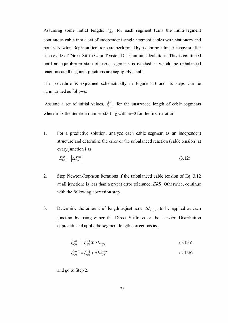
Assuming some initial lengths [0]( )u il for each segment turns the multi-segment

continuous cable into a set of independent single-segment cables with stationary end

points. Newton-Raphson iterations are performed by assuming a linear behavior after

each cycle of Direct Stiffness or Tension Distribution calculations. This is continued

until an equilibrium state of cable segments is reached at which the unbalanced

reactions at all segment junctions are negligibly small.

The procedure is explained schematically in Figure 3.3 and its steps can be

summarized as follows.

Assume a set of initial values, [ ]( )m

u il , for the unstressed length of cable segments

where m is the iteration number starting with m=0 for the first iteration.

1. For a predictive solution, analyze each cable segment as an independent

structure and determine the error or the unbalanced reaction (cable tension) at

every junction i as

[ ] [ ]( ) ( )m m

i iE T= ∆ (3.12)

2. Stop Newton-Raphson iterations if the unbalanced cable tension of Eq. 3.12

at all junctions is less than a preset error tolerance, ERR. Otherwise, continue

with the following correction step.

3. Determine the amount of length adjustment, ( )U iL∆ , to be applied at each

junction by using either the Direct Stiffness or the Tension Distribution

approach. and apply the segment length corrections as.

[ 1] [ ]( ) ( ) ( )m m

u i u i U il l L+ = ∆∓ (3.13a)

[ 1] [ ]( ) ( ) ( )m m segment

u i u i U il l L+ = + ∆ (3.13b)

and go to Step 2.

29

Plus or minus signs in Eq. 3.13a imply that if the unstressed length of cable

segment i is increased, that of the next segment i+1 is decreased by the same

amount. This way, the total unstressed length of cable system remains

unchanged.

Note that choosing the starting values for the unstressed length of each segment is a

crucial step. A good distribution of the cable length among its segments will decrease

the number of iteration considerably.

Figure 3.3 Newton Raphson method in schematic form for multi segment continuous

cable.

[2]M�

[1]M�

[0]M�

[ ]2T∆

[ ]1T∆

[ ]0T∆

T∆

[ ]2ul

[ ]1ul

[ ]0ul

ul

[ ]actual

ul

30

3.5 Comparison of Direct Stiffness and Relaxation Approaches.

In essence, both procedures described above can be used for the solution of multi-

segment continuous cables. They lead to an equilibrium state after a number of

iterations. However, as far as their effectiveness is concerned, there are certain

circumstances under which one of them is more effective than the other.

Tension distribution method is a discrete calculation method. A correction is applied

though a length adjustment at a joint to reduce the reaction imbalance at the relevant

support. The adjacent equilibrium states of cable segments are then recalculated.

After repeating similar length adjustments and calculations at all other internal

support locations, one round of calculations will be completed. At this point, the

cable system will be closer to its final equilibrium state. However, in general, the

cable system as a whole will not be in equilibrium since the correction applied at one

joint will upset the possible equilibrium state at the far ends of the cable segments

involved. Therefore, this predictive/corrective algorithm is applied cyclically at all

joints one by one until convergence is achieved at all support locations. On the other

hand, length adjustments in the correction phase are all applied simultaneously in the

Direct Stiffness approach. Then, all segments are reanalyzed and the convergence is

checked in the predictive phase for the next iteration.

Normally, if the length of a tight cable is decreased for a given segment, the end

reactions will increase. However if the length of a very slack cable is decreased, the

end reactions may also decrease. A cable having a changing length is supported

between two fixed supports will have minimum support reactions for a specific

length and the corresponding degree of slackness. The term very slack cable refers to

a cable with a degree of slackness beyond this limit. Therefore, based on this limit

state and for the purpose of analysis, a cable can be classified as either a tight or

slack cable or a very slack cable. These explanations could be easily seen in Figure

3.4. Curvature in Figure 3.4 is obtained for a cable having 0.05m diameter supported

at (0,0,0), (0,50,0) coordinates.

31

Figure 3.4 Typical slackness curve of a cable

Whether the Direct Stiffness or the Tension Distribution approach is used, a common

difficulty encountered in the analysis of slack cable systems is the overshooting

problem. The problem comes up when a cable segment turns into very slack cable

condition or just on the limit state in any iteration phase. In this case, the predicted

amount of length adjustment to be applied on these segments may become

excessively high since the calculations are based on the joint stiffnesses and

assumption of quasi-linear behavior of cable. This leads to oscillations between very

large corrections in either direction and finally divergence of the

prediction/correction iterations. In order to avoid the occurrence of such situations a

damping ratio of 0.5 is used in the correction step and half of the predicted

corrections are applied at the joints.

Although this damping ratio decreases the occurrence of those extreme situations, it

is still possible to see an extreme situation for some cable systems. So, corrections

should be checked in each iteration not to create a cable with a negative length.

Corrections are checked and revised for each joint in Tension Distribution method.

However, this revision is not possible for Direct Stiffness method, because Direct

Stiffness method finds corrections for the whole system. Therefore, if a problem is

32

encountered at a joint, revision of that joint correction should be distributed to all

segments. However, this could lead to problems at other joints and so on.

Stiffness matrix of the system will not be suitable if any one of the segments with the

highest degree of slackness turns into very slack cable state or around the limit state

in any iteration phase of calculation. Therefore stiffness method, which makes

calculations with the stiffness matrix of the whole system, is not appropriate for

systems which can have very slack cable segments. Tension distribution method is

better suited for such cable systems.

At the onset of analysis there are two options to choose as a solution procedure. One

choice is to start with the Direct Stiffness approach and switch to Tension

Distribution if a problem with the stiffness matrix and so corrections is detected.

Another choice is to decide on the degree of slackness of the cable system first

before proceeding with the initial cycle of corrections and continue accordingly. If

preliminary calculations reveal that the degree of slackness of multi-segment

continuous cable is less than a preset limit, the Direct Stiffness approach is utilized.

Otherwise, the subsequent iterations are continued with the Tension Distribution

approach.

Determination of the degree of slackness is not possible for multi segment

continuous cables although it is possible for single segment cables. Because

corrections and/or cable distribution to segments is not known in any iteration as

described above. In the software developed in this study for the analysis of multi-

segment continuous cable systems, CABPOS, the following approach is taken. Given

the total unstressed length of cable and the location of the support points, the total

length is distributed among the segments in proportion to their spans. An unstressed

length higher than 10% of the span is used as a limiting value for system to regard it

as a very slack cable This limit for the classification of a cable system as very slack

for the purpose of analysis appears to be a reasonable and safe value since no

difficulties are encountered with this assumed limit in the various sample analyses

carried out for verification.

33

The algorithm explained above for the solution of multi-segment continuous cables is

implemented in a FORTRAN program called CABPOS and used for the analysis of a

set of multi-segment continuous cable systems for verification.

34

CHAPTER 4

4. VERIFICATION FOR SINGLE-SEGMENT CABLES

4.1 General

Multi-segment continuous cable analysis algorithm is first used for the solution of

some single-segment cables for verification. The results obtained by the program

CABPOS are compared with those obtained by the widely used commercial finite

element program ANSYS [19]. The input data for ANSYS program of the sample

single-segment cable system is given in Appendix B1. The cable is analyzed in five

different configurations in space using a range of mesh densities. The final support

reactions and the cable geometry are used for comparison.

A numerical iterative algorithm is proposed for the solution of cable systems.

Consequently, the predicted solution will only be an approximation to the exact

equilibrium state. Therefore, the convergence characteristic of the algorithm as well

as its ability to produce the final equilibrium state accurately is of concern. The

convergence characteristic of the algorithm is verified by changing the cable

configuration in space and its degree of slackness. The accuracy of the predicted

results is checked by the mesh density used for the cable.

4.2 Description of the Problem

• Material properties of cable

Density of the cable : 7.85E3 kg/m3

Modulus of elasticity : 200E9 N/m

Thermal expansion coefficient : 1.2E-5 / ºC

35

• Physical properties of cable ;

Total cable length : 18 m

Diameter of cable : 0.05 m

• Environmental properties

Temperature change : +40 ºC

• Program constraint

Precision : 1E-6 m (ERR , the target error)

There are five different cable configurations. One of them is tight and the others are

slack cables. Support locations are given in Table 4.1. One end of cable is supported

at point A and other end is supported at point B. Each cable is solved for a range of

mesh densities of 50, 100, 250, 500, 1000 and 10000 elements.

Table 4.1 Support locations

Supports X coordinate

(m) Y coordinate

(m) Z coordinate

(m) A 0.0 0.0 0.0

B1 10.0 0.0 10.0

B2 9.0 3.0 11.0

B3 11.0 6.0 9.0

B4 11.0 9.0 11.0

B5 11.0 9.1 11.0

4.3 Solution by CABPOS

Data related with cable supported at A and B3 will be given in this section. Other

solutions will not be shown.

Final coordinates, length and reactions of cable A-B3 are shown in Table 4.2, Table

4.3, Table 4.4, Table 4.5, Table 4.6 and Table 4.7.

36

Table 4.2 Data for cable A-B3 solved with 50 elements.

Number of finite elements 50 Supports (m) A(0,0,0) B3(11,6,9)

X Coordinate (m) 0 10.9999994 Y Coordinate (m) 0 6.0000003 Z Coordinate (m) 0 8.9999996

Reactions (N) 1269.62 2216.84 Final Cable Length (m) 18.0087













37









The reaction data of cable A-B3 can be seen in Table 4.8.

Table 4.8 Support reactions for A-B3 given by CABPOS.

A-B3 Number of elements

First Support Reaction (N)

Second Support Reaction (N)

50 1269,62 2216,84 100 1277,81 2204,86 250 1282,75 2197,66 500 1284,40 2195,53 1000 1285,22 2194,05 10000 1285,97 2192,96

The convergence of the solution of cable A-B3 for different number of elements is

shown in Figure 4.1 and Figure 4.2.

38

Figure 4.1 Reactions at first support given by CABPOS.

Figure 4.2 Reactions at second support given by CABPOS.

39

It is seen in above figures that, reactions at supports converge to a value. There is a

0.6% error between 50 and 100 element solution. However, between 1000 and 10000

element solution, 0.06% error occurs. So, if this trend goes on, there would probably

be a 0.005% error for 100000 elements. Although it will converge a little to the real

value for reaction, this solution does not change reaction a lot.

4.4 Solution by ANSYS

ANSYS solve the problem as continuum between the end supports. Therefore, the

cable ends are always coincident with the supports.

Support reactions of cable A-B3 for different number of elements are given in Table

4.9

Table 4.9 Support reactions for cable A-B3 given by ANSYS.

A-B3 Number of Elements

First Support Reaction (N)


50 1285,97 2192,70 100 1286,03 2192,84 250 1286,04 2192,85 500 1286,05 2192,86 1000 1286,05 2192,86 10000 1286,05 2192,86

The convergence of the solution for different number of elements can be seen in

Figure 4.3 and Figure 4.4.

40

Figure 4.3 Reactions at first support given by ANSYS.

Figure 4.4 Reactions at second support given by ANSYS.

41

ANSYS gives approximately the correct results with a reasonable number of

elements. Slope of the convergence curve is zero from 1000 to 10000 elements, as

shown above. Zero slope means that there is no need to further refine the element

mesh.

4.5 Comparison of results

Comparison of solutions is made on reaction difference as said above. The

comparison could be made in a lot of different ways. However, stresses have much

importance for structural systems.

Convenient number of elements should be selected for each problem. It could be

made in a way that changing mesh density and comparing the results gotten from

each. 10000 elements is used for this problem, because, there won’t be much change

in result for further increase in finite element number.

Reaction results of each five configuration having 10000 elements are sorted in

Table 4.10.

Table 4.10 Reaction results for different configurations.

10000 elements First Support Reaction (N)


B1 CABPOS 1613,27 1613,50 ANSYS 1613,42 1613,42

B2 CABPOS 1416,98 1870,60 ANSYS 1417,06 1870,50

B3 CABPOS 1285,97 2192,96 ANSYS 1286,05 2192,86

B4 CABPOS 9993,01 11353,20 ANSYS 9993,24 11353,40

B5 CABPOS 302203,43 303577,66 ANSYS 302371,56 303744,94

42

Related error of percentages are tabulated in Table 4.11.

Table 4.11 Error of percentages for single-segment cable solutions.

Configurations First support error Second support error Maximum

error

A-B1 0,010% 0,005% 0,010%

A-B2 0,006% 0,006% 0,006%

A-B3 0,007% 0,005% 0,007%

A-B4 0,002% 0,002% 0,002%

A-B5 0,056% 0,055% 0,056%

It could be easily seen that there is very little difference between the solutions of

CABPOS and ANSYS. Average of maximum error of this problem is approximately

0.02%. It is known that both programs made errors related with finite element

number and rounding off. Another known matter is that structural systems are not

exquisite. So, 0.02% error is enough approximation for this type of problems.

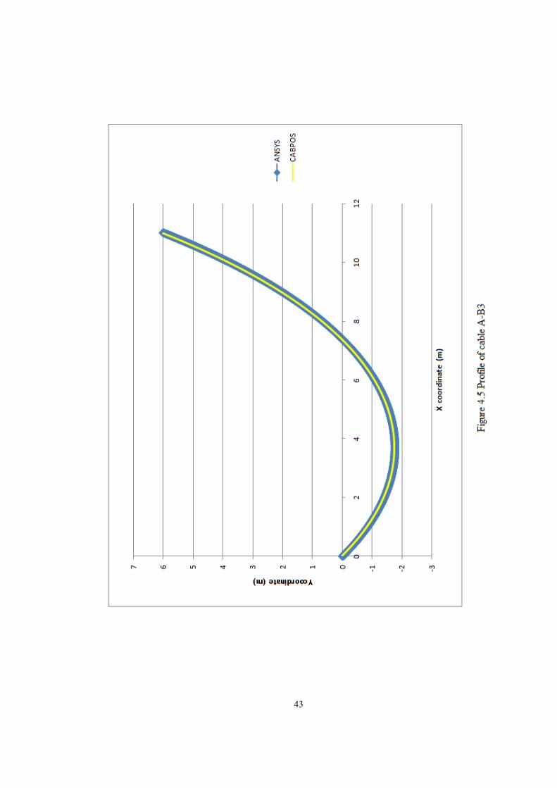
Profile of cable A-B3 is given in Error! Reference source not found. by the

coordinates obtained from both programs CABPOS and ANSYS.

43

Figure 4.5 Profile of cable A-B3

44

CHAPTER 5

5. VERIFICATION FOR MULTI-SEGMENT CONTINUOUS CABLES

5.1 General

The solution methods for multi-segment continuous cable are explained in Chapter 3.

According to these methods, if single-segment cable solution of CABPOS is correct

or approximately correct, the multi-segment continuous cable solution can be

verified by solving cable segment by segment. Reactions of each segment could be

found by single-segment cable solution of CABPOS with the lengths found from

multi-segment solution of CABPOS. Thus, reactions of successive segments can be

compared whether they are same. Although this technique could be called a valid

verification, ANSYS is used for verification.

Problem is solved in ANSYS by using contact elements. These contact elements

have zero tangent stiffness. Thus, these contacts could be classified as roller

supports. Monolithic cable is modeled as fixed supported at both ends and roller

supports are defined between these fixed supports. Different cable configurations are

obtained by displacing the one end of cable. Code of the program written in ANSYS

is given on Appendix B2.

The verification of multi-segment continuous cable solution is made on support

reactions as made in single-segment verification. All contact reactions and fixed

support reactions are compared.

5.2 Description of Problem

Cable having 0.05 m diameter was used in single-segment solution verification.

Cable is assumed 0.02 m diameter having an ice cover through the cable for multi-

segment continuous cable verification. The ice cover has a 0.05 diameter from the

45

center of the cable. So, this ice cover gives an extra load. This extra load is applied

by increasing density of cable which corresponds to 4 times density of steel.

• Material properties of cable ;

Weight of the cable : 4*7.85E3 kg/m3 (including ice)

Modulus of elasticity : 200E9 N/m

Thermal expansion coefficient : 1.2E-5 / ºC

• Physical properties of cable ;

Total cable length : 76.2 m

Diameter of cable : 0.02 m

• Environmental properties ;

Thermal change : +40 ºC

• Program constraint ;

Precision : 1E-6 m (ERR , the target error.)

There are 3 different cable configurations. One of them is tight and others are slack

cables. These different cable configurations are obtained by giving displacement to

one end of the cable. Coordinates of supports are shown in Table 5.1

Solutions of three different cable configurations are made for different number of

finite elements which are 100, 500, 1000 and 5000. Data related with cable supported

at F1 and F2c will be shown on this section.

46

Table 5.1 Coordinates of supports.

Supports Coordinates (m)

X Y Z

F1 0 0 0

R1 10 -1 0

R2 20 -3 0

R3 30 -6 0

R4 40 -10 0

R5 50 -15 0

R6 60 -21 0

F2a 70 -21 0

F2b 70 -27 0

F2c 70 -28 0

5.3 Solution of CABPOS

The reaction data of cable F1- F2c solved by CABPOS can be seen in Table 5.2.

Table 5.2 Support reactions of cable F1-F2c given by CABPOS.

F1-F2c Number of elements 100 500 1000 5000

Sup

port

rea

ctio

ns (

N) F1 224218,18 224219,66 224219,83 224219,97

R1 22846,55 22854,39 22855,37 22856,15 R2 22007,92 22015,76 22016,74 22017,52 R3 20861,23 20869,06 20870,04 20870,82 R4 19509,22 19517,046 19518,02 19518,80 R5 18051,54 18059,36 18060,33 18061,11 R6 16571,70 16579,51 16580,49 16581,27 F2c 221520,18 221521,53 221521,69 221521,81

The convergence of the solution for different mesh densities is shown in Figure 5.1.

Sum of the reactions vs. number of finite elements is graphed instead of showing

graph for each support.

47

Figure 5.1 Sum of support reactions for cable F1-F2c given by CABPOS.

The reaction difference between 1000 and 5000 element solution is approximately 5

N. This difference corresponds to 0.0006% error which means that 5000 element is

enough for this problem.

5.4 Solution of ANSYS

The reaction data of cable F1- F2c solved by ANSYS can be seen in Table 5.3.

Table 5.3 Support reactions of cable F1-F2c given by ANSYS.

F1-F2c Number of elements 100 500 1000 5000

Sup

port

Rea

ctio

ns (

N) F1 226230,43 224685,73 224448,29 224270,94

R1 23037,47 22980,46 22920,09 22867,71 R2 22689,94 22053,53 22058,93 22021,56 R3 20718,40 20975,65 20870,25 20878,30 R4 19763,40 19510,54 19548,75 19527,77 R5 18350,37 18049,64 18042,16 18059,45 R6 16624,45 16686,45 16648,23 16591,25 F2c 223536,87 221968,07 221744,43 221583,08

48

The convergence of the solution for different number of elements is shown in Figure

5.2.

Figure 5.2 Sum of support reactions for cable F1-F2c given by ANSYS.

There is 481N difference between 1000 and 5000 element solution. This corresponds

to 0.085% error.

5.5 Comparison

Comparison is made in the same way as in chapter 4. Maximum number of element,

which is 5000, is used for solution of both programs. Reactions at supports are

compared for all configurations.

Reaction results of each three configuration having 5000 elements are sorted in Table

5.4, Table 5.5 and Table 5.6.

49

Table 5.4 Support reactions for cable F1-F2a.

F1-F2a Solution types CABPOS ANSYS

Sup

port

rea

ctio

ns (

N) F1 2861,03 2859,14

R1 1239,51 1240,29 R2 1212,78 1212,07 R3 1177,38 1177,65 R4 1139,48 1139,42 R5 1118,15 1118,53 R6 596,13 596,49 F2a 831,34 831,01

Table 5.5 Support reactions for cable F1-F2b.

F1-F2b Solution types CABPOS ANSYS

Sup

port

rea

ctio

ns (

N) F1 4621,47 4618,39

R1 1408,52 1408,76 R2 1374,28 1374,32 R3 1327,64 1327,74 R4 1273,07 1272,53 R5 1215,29 1215,65 R6 977,02 977,30 F2b 2011,53 2008,40

Table 5.6 Support reactions for cable F1-F2c.

F1-F2c Solution types CABPOS ANSYS

Sup

port

rea

ctio

ns (

N) F1 224219,97 224270,94 R1 22856,15 22867,71 R2 22017,52 22021,56 R3 20870,82 20878,30 R4 19518,80 19527,77 R5 18061,12 18059,45 R6 16581,27 16591,25 F2c 221521,81 221583,08

50

Related percentages of errors are tabulated below in Table 5.7.

Table 5.7 Error of percentages for single-segment cable solution.

Error of percentages

Supports Cable configurations

F1-F2a F1-F2b F1-F2c F1 0,0664% 0,0666% 0,0227% R1 0,0633% 0,0165% 0,0505% R2 0,0586% 0,0029% 0,0183% R3 0,0232% 0,0078% 0,0358% R4 0,0067% 0,0429% 0,0459% R5 0,0340% 0,0301% 0,0092% R6 0,0611% 0,0291% 0,0602% F2 0,0402% 0,1555% 0,0277%

ANSYS and CABPOS give approximately same results for all cable configurations.

Average errors for F1-F2a, F1-F2b and F1-F2c configurations are 0.0442%, 0.0439%

and 0.0338% respectively. These amounts of errors are admissible for a structural

member.

Profile of cables F1-F2a, F1-F2b and F1-F2c are shown in Error! Reference source

not found., Error! Reference source not found., Error! Reference source not

found. respectively.

51

Figure 5.3 Profile of cable F1-F2a

52

Figure 5.4 Profile of cable F1-F2b

53

Figure 5.5 Profile of cable F1-F2c

54

CHAPTER 6

6. COMPUTER PROGRAM: CABPOS (CABLE POSITIONING)

6.1 General

CABPOS is a program which is build for the purpose of analyzing and positioning of

cables having different support conditions. Lots of routines have been written by

programmers in the past. Those programs analyze only the single-segment cable

problems having 2 fixed supports at the ends of the cable. CABPOS is a further

program for cable analysis. It analysis not only the single-segment cables but also the

multi-segment continuous cables. Multi-segment continuous cable is a cable which is

supported by two fixed support at both ends, in addition, it is supported by roller

supports between the ends.

FORTRAN programming language is used for building CABPOS. It is based on a

main program which runs many subroutines. Main program and subroutines will be

introduced later. Before these, main procedure will be defined. Code of CABPOS is

given on Appendix A.

6.2 Procedure

Basically, program has three input and five output text files. Program gets the cable

properties, environment conditions, coordinates of supports and data for modulus of

elasticity from input and gives the nodal coordinates of cable, support reactions, final

coordinates of roller supports, lengths for each segment and end forces of cable for

each segment. In those input text files data should be written in consistent units.

Solution is found by two methods. These are direct stiffness method and tension

distribution method. Direct stiffness method is used for tight cable and tension

distribution method is used for slack cable problems. Although tension distribution

55

method solves both problems, it takes lots of time for solution. Besides, direct

stiffness method could not solve slack cable problems, because of a property of cable

explained before.

Principle of direct stiffness method is basis on changing length of each segment.

Change in reaction difference of cable on each support is found by changing length

of each segment. Stiffness matrix is formed by the data of change in reaction

difference of cable on each support. The increment of length for each segment is

found form stiffness matrix analysis. This procedure is made several iterations of

Newton-Raphson method, because of nonlinear behavior of cable.

Principle of tension distribution method is same as direct stiffness method. Stiffness

method makes a total calculation on the other hand; tension distribution method

makes calculations between two successive segments. It founds the increment of

length for successive segments by changing the length of cables connected on a roller

support. This calculation is made for each roller support.

6.3 Main Program

The main program of CABPOS get the input data from the text file and checks

whether the system is a single-segment cable problem or multi-segment continuous

cable problem. Accordingly it leads. Then it checks whether the cable is tight or

slack. After that classification of the problem, program runs the subroutines

MSPFTC and MSPFSC respectively.

Operation of checker for tightness basis on a simple principle; It firstly, calculate the

total direct length of the path, which cable should keep, by the subroutine

COTLOES. Secondly, it checks whether total cable length is greater than 1.1 times

of total direct length of the path. The number 1.1 is an experimental constant made

on this computer program.

MSPFTC is a subroutine for direct stiffness method MSPFSC is a subroutine for

tension distribution method. After the solution of main subroutines MSPFTC and

MSPFSC, program gives the output.

56

Subroutines used in main program are:

• MSPFTC(LOES,NOS,DOC,WOC,MOE,TEC,TC,PLP,FEN,SX,SY,SZ,X,Y,

Z,FLOC,R)

• MSPFSC(LOES,NOS,DOC,WOC,MOE,TEC,TC,PLP,FEN,SX,SY,SZ,X,Y,

Z,FLOC,R)

• INPUT1(TCL,NOS,DOC,WOC,MOE,TEC,TC,PLP,FEN)

• INPUT2(NOS,SX,SY,SZ)

• COTLOES(NOS,SX,SY,SZ,TLOES,TTLOC)

• COSCLOES(NOS,TLOES,TTLOC,TCL,LOES)

• DOS(NOS,SY,TLOES,TCL,TTLOC,LOES)

• ALAI(NOS,IOLFT,IIOL,LOES)

• AIOES(l,NOS,IIOL,LOES)

• AIOESS(k,l,NOS,IIOL,LOES)

• ACOFPFES(k,NOS,CC,C1,C2)

• COOS(k,l,NOS,X1,Y1,Z1,X2,Y2,Z2,CL,DOC,WOC,MOE,TEC,TC,PLP,FE

N,X,Y,Z,FLOC,R,IR)

• GIFTFP(X1,X2,Z1,Z2,SR)

• ACOFP(X1,Y1,Z1,IX,IY,IZ)

• ARAIOFP(SR,IIOR,IRX,IRY,IRZ,IR)

• FEC(i,WOC,FEN,FEL,MOE,AOC,TEC,TC,IR,IRX,IRY,IRZ,IX,IY,IZ,IFLO

C)

• FMEC(FEN,IX,IY,IZ,IXX,IXY,IXZ,IYX,IYY,IYZ,IZX,IZY,IZZ,X2,Y2,Z2,

FM,DTT)

57

• FRM(l,k,NOS,FEN,IR,R1,RLP)

• FRMS(l,k,NOS,FEN,IR,R1,RLP)

• TIB(l,NOS,IIOL,LOES)

• TIBS(l,k,NOS,IIOL,LOES)

• SMS(NOS,R1,RLP,DR,DDR)

• MATINV(NSTRE,AMATX)

• MATMULT(NSTRE,MATX1,MATX2,MATX3)

• OUTPUT1(NOS,FEN,X,Y,Z,FLOC,R)

• ICAAI(i,NOS,IIOL,R1,RLP,LOES)

• SOD(l,k,i,NOS,FEN,IX,IY,IZ,IR,IFLOC,X,Y,Z,R,FLOC)

• MODULUS(STRESS,STRAIN)

• OUTPUT2(NOS,FEN,X,Y,Z,FLOC,R)

6.4 Subroutines

Some of the subroutines, which are important, are introduced. The functions of those

subroutines are explained. Some important variables are given by their definitions.

6.4.1 MSPFTC

MSPFTC is a subroutine which gives solution for tight cable problems. Program

inputs are initial length of cable of each segment, material and coordinate properties

of cable. Outputs are nodal coordinates of cable, final length of cable of each

segment and nodal reactions of cable. Program runs using nested three loops. First

one is iteration loop, second one is incrementation loop and the last one is segment

loop.

Under the control of iteration loop stiffness matrix calculations are made by

subroutines SMS, MATINV and MATMULT. After matrix calculations, check for

58

the reaction differences between successive segments is made. If check fails, new

lengths will be assigned by subroutine ALAI.

Assigning increment and taking them back is made by subroutines AIOES and TIB

in incrementation loop.

In the segment loop, firstly, coordinates of first and last point of each segment are

assigned by subroutine ACOFPFES. Secondly it runs the subroutine COOS which

makes one segment calculation. Finally, first and last nodal reactions are formed.

Variable Definition

R1 Reaction of first point of each segment.

RLP Reaction of last point of each segment.

DR Reaction difference between successive cables on each roller

support for each increment.

DDR Change in DR between nonincremented solution and

incremented solution on each roller support for each iteration.

IOLFT Solution for change in length for each segment.

6.4.2 MSPFSC

Work done by MSPFSC is same with MSPFTC, however, procedures are different.

MSPFSC is a subroutine which gives solution for slack cable problems. Program

inputs are initial length of cable of each segment, material and coordinate propeties

of cable. Output is nodal coordinates of cable, final length of cable of each segment

and nodal reactions of cable. Program runs using nested three loops. First one is

iteration loop, second one is roller support loop and the last one is successive

segments’ loop.

Iteration loop only checks whether the reaction difference between successive

segment cables are greater than precision needed. If check fails, iteration will goes

on.

59

Change in length between two successive supports is calculated and length of each

segment is renewed in Roller support loop.

The last loop is successive segments loop which makes calculations for analysis of

successive segments connected by a roller support. This loop has two steps. In the

first step, it analyzes two successive supports by nonincremented cable lengths. In

the second step, same calculations are made for incremented cable lengths.

Variable Definition

R1 Reaction of first point of each segment.

RLP Reaction of last point of each segment.

INCR Solution for change in length for each segment.

6.4.3 INPUT1

INPUT1 gathers the information from the text file about cable properties. Those

cable properties and their variable names in program code are as follows.

Variable Definition

NOS Number of segment.

FEN Finite element number.

TCL Total cable length.

DOC Diameter of cable.

WOC Weight of cable per length.

MOE Modulus of elasticity.

PLP Precision for second support coordinates.

TEC Thermal expansion coefficient.

TC Temperature change.

60

6.4.4 INPUT2

This subroutine gathers the coordinates of two fixed supports and roller supports.

Fixed supports should be written in first row and last row in the text file. The data

between those fixed support data are coordinates of roller supports. Additionally,

cable will be positioned in the order of supports written in the text file.

6.4.5 COTLOES

This subroutine calculates the direct length of the path of the cable. It gives total

direct length of the cable path and direct length of each segments’ cable path.

Variable Definition

TLOES Direct length of each segments’ cable path.

TTLOC Total direct length of cable path.

6.4.6 COSCLOES

Initial cable lengths must be given for solution. COSCLOES calculates the initial

cable lengths for each segment to start the calculation. Total cable length is

distributed to each segment proportional to their direct length of cable path.

Variable Definition

LOES Length of cable of each segment.

6.4.7 DOS

Most of the sag of the cable would be occur on the segment having less elevation. In

other words, cable will slip on the roller supports to the lower elevations.

This subroutine gives whole sag of the cable to the segment which has the less

elevation. It renews the initial length of cable of each segment. The aim of this renew

is to decrease the iteration number of the program.

61

Variable Definition

MINCOOR Index for segment having minimum elevation. This elevation

is calculated by the sum of y coordinates of two supports of a

segment.

6.4.8 ALAI

This subroutine adds the calculated increment to the cable length of each segment.

6.4.9 AIOES

This subroutine gives the imaginary increment in length of each segment.

6.4.10 COOS

COOS is the main subroutine of the program. It makes the calculations of one

segment. Inputs are coordinates of supports of one segment and material properties

of cable. Outputs are nodal coordinates, final cable length after deformation and

nodal reactions. COOS runs with two nested loop. First one is iteration loop, second

one is finite element loop.

As previously introduced in chapter 2, initial reaction of first node of cable is given

by GIFTFP to make the system determinant. Imaginary increment is applied to this

reaction in all three directions in incrementation loop. Flexibility matrix is formed by

FMEC by data calculated by finite element loop. Increment for each direction is

calculated and added to the initial reaction by flexibility matrix calculations. Finally,

check is made for last node’s coordinate whether it is approximately close to the

second support of the segment.

After incrementation made in incrementation loop finite element loop processes and

gives the nodal coordinates and reactions, and also final node’s coordinates. This

process is made four times. First one is for nonincremented reaction solution and the

other three is for incremented reaction solution for three global directions.

62

Variable Definition

FEL Finite element length: This length will change segment to

segment. However FEN is constant for each segment.

SR Initial reaction of first node of each segment which is renewed

after each iteration.

DRR Increment of reaction for each direction calculated by

flexibility matrix.

6.4.11 GIFTFP

Giving initial reactions for segment calculations is made by this subroutine. An

approximate initial reaction decreases the iteration number of program. However, it

is very hard to predict the initial reaction of cable approximately. So, GIFTFP gives a

small reaction according to its orientation. In other words, this subroutine only

determines the direction of the reaction and assigns it.

6.4.12 FEC

Finite element calculations are made by FEC. Nodal coordinates and reactions are

calculated in this subroutine.

Variable Definition

STRAIN Strain of a finite element.

DELTA Elongation of a finite element.

6.4.13 FMEC

This subroutine forms the flexibility matrix of one segment. It uses coordinates of

final node. This coordinates are for incremented and nonicremented reactions.

Variable Definition

IX, IY, IZ Coordinates of final node for nonicremented reaction case.

IXX, IXY, IXZ Coordinates of final node for incremented reaction of X

direction.

63

IYX, IYY, IYZ Coordinates of final node for incremented reaction of Y

direction.

IZX, IZY, IZZ Coordinates of final node for incremented reaction of Z

direction.

SOL Approximation for final node of the segment.

6.4.14 MATINV

Matrix inversion is made by MATINV. The given square matrix is renewed by the

inverse of it.

Variable Definition

NSTRE Dimension of matrix.

AMATX Matrix to be inverted.

6.4.15 MATMULT

Multiplication of a square matrix FM1, having dimension NOS1, by vector SOL1

having same dimension gives vector DRR1.

6.4.16 OUTPUT1

OUTPUT1 gives the information about final cable position and forces. Those outputs

are as follows.

Variable Definition

NOS Number of segment.

FEN Finite element number.

X,Y,Z Coordinates of each finite element.

FLOC Final length of cable.

R Reaction of each finite element.

64

6.4.17 MODULUS

This subroutine gets the stress strain data of cable from INPUT3 text file. Then find

the strain value for corresponding stress value for each finite element by

interpolation.

Variable Definition

STRESS Stress data.

STRAIN Strain data.

65

CHAPTER 7

7. SUMMARY, CONCLUSIONS AND RECOMMENDATIONS

7.1 Summary

Cables are highly nonlinear structural members under transverse loading. This

nonlinearity is mainly due to the close relationship between the final geometry under

transverse loads and the resulting stresses in its equilibrium state rather than the

material properties. In practice, the cables are usually used as isolated single-segment

elements fixed at the ends. Various studies and solution procedures suggested by

researchers are available in the literature for such isolated cables. However, not much

work is available for continuous cables with multiple supports.

In this study, a multi-segment continuous cable is defined as a cable fixed at the ends

and supported by a number of stationary roller supports in between. Total cable

length is assumed constant and the intermediate supports are assumed to be

frictionless. Therefore, the critical issue is to find the distribution of the cable length

among its segments in the final equilibrium state. Since the solution of single-

segment cables is available the additional condition to be satisfied for multi-segment

continuous cables with multiple supports is to have stress continuity at intermediate

support locations where successive cable segments meat. A predictive/corrective

iteration procedure is proposed for this purpose. The solution starts with an initially

assumed distribution of total cable length among the segments and each segment is

analyzed as an independent isolated single-segment cable. In general, the stress

continuity between the cable segments will not be satisfied unless the assumed

distribution of cable length is the correct distribution corresponding to final

equilibrium state. In the subsequent iterations the segment lengths are readjusted to

eliminate the unbalanced tensions at segment junctions. The iterations are continued

until the stress continuity is satisfied at all junctions. Two alternative approaches are

66

proposed for the segment length adjustments: Direct stiffness method and tension

distribution method.

A computer program called CABPOS is developed for the analysis of multi-segment

continuous cables and both techniques have been implemented into it. The program

is coded in FORTRAN. The total length of the cable, material properties, the load

and environmental data, support locations and the desired density for the finite

element mesh is supplied to the program by the user. The program then generates the

geometry of cable segments, internal stresses and the support reactions in the final

equilibrium state. A brief description of the program CABPOS is given in chapter 6.

Verification of the solutions generated by CABPOS is made by comparing the results

with ANSYS. The results are satisfactory and compares well with those obtained by

the commercial finite element program ANSYS. .In the ANSYS solution, the roller

supports are defined as dimensionless and they are modeled as contact elements. The

friction is eliminated for the contact elements by setting the tangent stiffness of the

contact to zero.

7.2 Conclusions

Based on the research carried out in this study and the experienced gained from the

analysis of various verification examples, the conclusions drawn can be summarized

as follows:

• A solution procedure is devised for the analysis of multi-segment continuous

cables with multiple supports. In general, a predictive/corrective iterative

algorithm coupled with Newton-Raphson iterations is employed for the

nonlinear analysis. The proposed algorithm is tested with a number of

verification examples and satisfactory results are obtained.

• The behavior of slack cables is characteristically different from that of tight

cables because of the order-of-magnitude difference between the cable

stiffnesses in each case. Therefore, there is a need for a specific treatment for

each case. Two alternative techniques are proposed for this purpose: Direct

Stiffness method and Tension/Length Distribution method. The former is best

67

suited for tight cables whereas the latter is more appropriate for slack cables.

The Tension/Length Distribution approach even becomes the only choice as

the degree of slackness of the cable or any segment of it increases.

• The use of Tension/Length Distribution approach unnecessarily increases the

correction iterations and the use of the Direct Stiffness method causes some

wild oscillations or even divergence before reaching the equilibrium state.

Therefore, a proper combination of the two techniques is necessary for a

general solution algorithm. For this purpose, a smart algorithm for the

detection of excessive slackness in a given configuration of a cable is critical.

7.3 Recommendations for future studies

Although verification is made and results show that solutions are almost correct.

Some assumptions and simplifications are made to reach the solution. Those are:

• Modulus of elasticity of the cable is assumed constant for verification.

Although there is an input text files for modulus of elasticity data. There must

be experimental data of a cable to use this property of CABPOS.

• Friction of the cable on roller supports is assumed zero. Thus equality of

cable tensions on each roller support is enough for static equilibrium.

• Flexural rigidity of cable is assumed zero. Because, the cables used in

structural systems are long enough to neglect flexural rigidity.

• 1.1 times the span of multi-segment continuous cable is used as a limit for

classification of system as very slack cable.

• There are some assumptions due to finite element modeling like similars

have.

68

Therefore, some recommendations are given for further research;

• CABPOS has tool for variable modulus of elasticity. This tool could be run

by using stress-strain data of a cable and verification could be made by a

computer program.

• Some friction could be applied on roller supports and also verification could

be made with a computer program.

• Flexural and shear rigidities can be considered in analysis. Although it does

not affect large scale systems, there would be effect on small scale cable

systems.

• Verification of the proposed methods can be made experimentally.

• Although there is a research about the degree of slackness of a single-segment

cable in this thesis, this study is superficial. Therefore, a parametric study

about the degree of slackness can be carried out.

• An empirical value of 1.1 is determined by experiences obtained through the

solution of sample problems. This number can be revised by some well

settled studies or another way to determine the degree of slackness of multi-

segment cable can be found.

69

REFERENCES

[1] Costello, G.A., 1987, “Theory of wire rope,” Springer.

[2] Kumar, K., Cochran. J.E., 1987, “Closed-form analysis for elastic

deformations of multilayered strands”, J. Appl. Mech., 54, pp. 893-903.

[3] Dishinger, F., 1949, “Hängebrücken fur Schweste Verkehrslasten”, Der

Bauingenieur 24, S.65 und S.107.

[4] Ernst, H.J., 1965, “Der E-Modul von Seilen unter Brucksichtigung des

Durchhangers”, Der Bauingenieur, 40(2), pp. 52-55.

[5] Hajdin, N., Michaltsos, G.T., Konstantakopoulos, T.G., 1998, “About the

equivalent modulus of elasticity of cables of cable-stayed bridges”, Sci. J.

Facta Universitatis, Arc and Civil Eng series, Vol.1, No. 5, pp. 569-575.

[6] Turner, M.J., Clough, R.W., Martin, H.C., Topp. L.J., 1956, “Stiffness and

deflection analysis of complex structures”, Journal of Aeronautical Sciences,

Vol. 23, pp. 805-823.

[7] Madenci, E., Güven Đ., 2006, “The finite element method and applications in

engineering using ANSYS”, Springer.

[8] Clough, R.W., 1960, “The finite element method in plane stress analysis”,

Proceedings, 2nd Conference on electronic computation, ASCE. Structural

division, Pittsburg, Pennsylvania.

[9] Micholas, J., Brinstiel, C., 1962, “Movements of cables due to changes in

loading”, Transactions ASCE, 127, pp. 267-303.

70

[10] Skop, R.A., O’Hara, G.J., 1970, ”The Method of Imaginary Reactions : A

New Technique for Analyzing Structural Cable Systems”, Marine

Technology Society Journal, 4, pp. 21-30.

[11] Skop, R.A., O’Hara, G.J., 1970, ”A Method for the Analysis of Internally

Redundant Strucutal Cable Arrays”, Marine Technology Society Journal, 6,

pp. 6-18.

[12] Polat, M.U., 1981, “Nonlinear Computer Analysis of Guyed Towers and

Cables”, M.S. thesis, Middle East Technical University, Ankara, Turkey.

[13] Peyrot, A.H., Goulois, A.M., 1979, “Analysis of cable structures”, Computers

& Structures, 10, pp. 805-813.

[14] Fleming, J.F., 1979, ”Nonlinear static analysis of cable-stayed bridge

structures”, Computers & Structures, 10, pp. 621-635.

[15] Charland, J.W., Hernried, A.G., Pyles, M.R., 1994, “Cable systems with

elastic supporting elements”, Journal of Structural Engineering ASCE, 120,

pp. 3649-3665.

[16] Aufaure, M., 2000, “A three-node cable element ensuring the continuity of

the horizontal tension; a clamp-cable element”, Computers & Structures, 74,

pp. 243-251.

[17] Kwang Sup Chung, Jae-Yeol Cho, Jung II Park, Sung-Pil Chang, 2011,

“Three-Dimensional Elastic Catenary Cable Element Considering Sliding

Element”, Journal of Engineering Mechanics ASCE, 137, pp. 276-283.

71

[18] Kyoung-Bong, H., Sun-Kyun P., 2005, “Parametric Study of Truss Bridges

by the Post-Tensioning Method”, Canadian Journal of Civil Engineers, 32,

pp. 420-429.

[19] Mechanical APDL (ANSYS) Version 21.1 Academic Teaching Advanced

Utility Menu

72

APPENDICES

APPENDIX A

CODE OF CABPOS

!NOS : NUMBER OF SEGMENT

!FEN : FINITE ELEMENT LENGTH

!TCL : TOTAL CABLE LENGTH

!DOC : DIAMETER OF CABLE

!WOC : WEIGTH OF CABLE

!MOE : MODULUS OF ELASTICITY

!TEC : THERMAL EXPANSION COEFFICIENT

!TC : THERMAL CHANGE

!PLP : PRECISION OF LAST POINT

!SX,SY,SZ : COORDINATES OF EACH SUPPORT

!X,Y,Z : COORDINATES OF EACH SEGMENT AND EACH FINITE ELEMENT

!FLOC : FINAL LENGTH OF CABLE OF EACH SEGMENT

!R : REACTION OF EACH SEGMENT AND EACH FINITE ELEMENT

!IR : IMAGINARLY NONINCREMENTED REACTIONS OF EACH SEGMENT

!TTLOC : TOTAL TRAPEZOIDAL LENGTH OF CABLE

!TLOES : TRAPEZOIDAL LENGTH OF EACH SEGMENT

!LOES : LENGTH OF EACH SEGMENT

INTEGER NOS,FEN

DOUBLE PRECISION TCL,DOC,WOC,MOE,TEC,TC,PLP

DOUBLE PRECISION SX(100),SY(100),SZ(100)

DOUBLE PRECISION X(100,10000),Y(100,10000),Z(100,10000),FLOC(100),R(100,10000),IR(10000)

73

DOUBLE PRECISION TTLOC,TLOES(100),LOES(100)

!INPUT1 DATA

CALL INPUT1(TCL,NOS,DOC,WOC,MOE,TEC,TC,PLP,FEN)

!INPUT2 DATA

CALL INPUT2(NOS,SX,SY,SZ)

!CHECK FOR SINGLE SEGMENT

IF (NOS.NE.1) GOTO 63

CALL COOS(1,1,NOS,SX(1),SY(1),SZ(1),SX(2),SY(2),SZ(2),TCL,DOC,WOC,MOE,TEC,TC,PLP,FEN,X,Y,Z,FLOC,R,IR)

CALL OUTPUT1(NOS,FEN,X,Y,Z,FLOC,R)

GOTO 64

63 CONTINUE

!CALCULATION OF TRAPEZOIDAL LENGTH OF EACH SEGMENT

TTLOC=0

CALL COTLOES(NOS,SX,SY,SZ,TLOES,TTLOC)

!CALCULATION OF STARTING CABLE LENGTH OF EACH SEGMENT

CALL COSCLOES(NOS,TLOES,TTLOC,TCL,LOES)

!CHECK FOR TIGHT OR SAG CABLE

IF(TCL.GT.TTLOC*1.1)GOTO 52

!MULTISEGMENT PROGRAM FOR TIGHT CABLE

CALL MSPFTC(LOES,NOS,DOC,WOC,MOE,TEC,TC,PLP,FEN,SX,SY,SZ,X,Y,Z,FLOC,R)

GOTO 53

52 CONTINUE

!DETERMINATION OF SAG

CALL DOS(NOS,SY,TLOES,TCL,TTLOC,LOES)

!MULTISEGMENT PROGRAM FOR SAG CABLE

74

CALL MSPFSC(LOES,NOS,DOC,WOC,MOE,TEC,TC,PLP,FEN,SX,SY,SZ,X,Y,Z,FLOC,R)

53 CONTINUE

!OUTPUT1 DATA



64 CONTINUE

END

!!!!!!!!!!!!!!!!!!!!!!!!!!!!!!!!!!!!!!!!!!!!!!!!!!!!

!SUBROUTINE FOR MULTISEGMENT PROGRAM FOR TIGHT CABLE

!!!!!!!!!!!!!!!!!!!!!!!!!!!!!!!!!!!!!!!!!!!!!!!!!!!!



!X1,Y1,Z1 : FIRST COORDINATE OF SEGMENT

!X2,Y2,Z2 : SECOND COORDINATE OF SEGMENT

!CL : CABLE LENGTH OF SEGMENT







!SX,SY,SZ : SUPPORT COORDINATES


!IIOL : IMAGINARY INCREMENTATION ON LENGTH

!IOLFT : INCREMENTATION OF LENGTH


75




!R1 : FIRST REACTION OF EACH SEGMENT AND INCREMENTATION

!RLP : LAST REACTION OF EACH SEGMENT AND INCREMENTATION

!DR : REACTION DIFFERENCE ON EACH SUPPORT

!DDR : CHANGE IN REACTION DIFFERENCE ON EACH SUPPORT FOR EACH INCREMENTATION

SUBROUTINE MSPFTC(LOES,NOS,DOC,WOC,MOE,TEC,TC,PLP,FEN,SX,SY,SZ,X,Y,Z,FLOC,R)

INTEGER NOS,FEN

DOUBLE PRECISION X1,Y1,X2,Y2,Z1,Z2,CL,DOC,WOC,MOE,TEC,TC,PLP

DOUBLE PRECISION SX(NOS+1),SY(NOS+1),SZ(NOS+1),LOES(NOS)

DOUBLE PRECISION IIOL,IOLFT(NOS-1,1)

DOUBLE PRECISION X(NOS,FEN+1),Y(NOS,FEN+1),Z(NOS,FEN+1),R(NOS,FEN+1),FLOC(NOS)

DOUBLE PRECISION IR(FEN+1),R1(NOS,NOS),RLP(NOS,NOS)

DOUBLE PRECISION DR(NOS-1,NOS),DDR(NOS-1,NOS-1)

IIOL=0.000001

DO 48 i=1,(NOS-1)

IOLFT(i,1)=0

48 CONTINUE

!ITERATION LOOP

DO 19 m=1,100

!ASSIGNING LENGTH AND INCREMENTATION

CALL ALAI(NOS,IOLFT,IIOL,LOES)

!INCREMENTATION LOOP

DO 20 l=1,NOS

!ASSIGNING INCREMENTATION ON EACH SUPPORT

76

CALL AIOES(l,NOS,IIOL,LOES)

!SEGMENT LOOP

DO 22 k=1,NOS

!ASSIGNING COORDINATES OF FIRST POINT FOR EACH SEGMENT

CALL ACOFPFES(k,NOS,SX,X1,X2)

CALL ACOFPFES(k,NOS,SY,Y1,Y2)

CALL ACOFPFES(k,NOS,SZ,Z1,Z2)

!CALCULATION OF ONE SEGMENT

CL=LOES(k)

CALL COOS(k,l,NOS,X1,Y1,Z1,X2,Y2,Z2,CL,DOC,WOC,MOE,TEC,TC,PLP,FEN,X,Y,Z,FLOC,R,IR)

!FORMING REACTION MATRICE

CALL FRM(l,k,NOS,FEN,IR,R1,RLP)

22 CONTINUE

!TAKING INCREMENTATION BACK

CALL TIB(l,NOS,IIOL,LOES)

20 CONTINUE

!FORMING STIFFNESS MATRICE

CALL SMS(NOS,R1,RLP,DR,DDR)

!STIFFNESS MATRICE INVERSION

CALL MATINV((NOS-1),DDR)

!MATRICE MULTIPLICATION

CALL MATMULT((NOS-1),DDR,DR,IOLFT)

!CHECK FOR REACTION PRECISION

DO 47 n=1,(NOS-1)

IF((RLP(1,n)-RLP(1,n)*PLP).LT.R1(1,n+1)) GOTO 30

GOTO 19

77

30 IF((RLP(1,n)+RLP(1,n)*PLP).GT.R1(1,n+1)) GOTO 47

GOTO 19

47 CONTINUE

GOTO 33

19 CONTINUE

33 CONTINUE

END

!!!!!!!!!!!!!!!!!!!!!!!!!!!!!!!!!!!!!!!!!!!!!!!!!!

!SUBROUTINE FOR MULTISEGMENT PROGRAM FOR SAG CABLE

!!!!!!!!!!!!!!!!!!!!!!!!!!!!!!!!!!!!!!!!!!!!!!!!!!



!X1,Y1,Z1 : FIRST COORDINATE OF SEGMENT

!X2,Y2,Z2 : SECOND COORDINATE OF SEGMENT

!CL : CABLE LENGTH OF SEGMENT







!SX,SY,SZ : SUPPORT COORDINATES







78



SUBROUTINE MSPFSC(LOES,NOS,DOC,WOC,MOE,TEC,TC,PLP,FEN,SX,SY,SZ,X,Y,Z,FLOC,R)

INTEGER NOS,FEN

DOUBLE PRECISION X1,Y1,X2,Y2,Z1,Z2,CL,DOC,WOC,MOE,TEC,TC,PLP

DOUBLE PRECISION SX(NOS+1),SY(NOS+1),SZ(NOS+1)

DOUBLE PRECISION IIOL,LOES(NOS)


DOUBLE PRECISION IR(FEN+1),R1(NOS,2),RLP(NOS,2)

IIOL=0.000001

!ITERATION LOOP

DO 100 m=1,1000

!SEGMENT LOOP

DO 101 k=1,(NOS-1)

!INCREMENTATION LOOP

DO 102 l=1,2

!ASSIGNING INCREMENTATION ON EACH SUPPORT

CALL AIOESS(k,l,NOS,IIOL,LOES)


CALL ACOFPFES(k,NOS,SX,X1,X2)

CALL ACOFPFES(k,NOS,SY,Y1,Y2)

CALL ACOFPFES(k,NOS,SZ,Z1,Z2)


CL=LOES(k)

CALL COOS(k,l,NOS,X1,Y1,Z1,X2,Y2,Z2,CL,DOC,WOC,MOE,TEC,TC,PLP,FEN,X,Y,Z,FLOC,R,IR)

79


CALL FRMS(k,l,NOS,FEN,IR,R1,RLP)


CALL ACOFPFES(k+1,NOS,SX,X1,X2)

CALL ACOFPFES(k+1,NOS,SY,Y1,Y2)

CALL ACOFPFES(k+1,NOS,SZ,Z1,Z2)


CL=LOES(k+1)

CALL COOS(k+1,l,NOS,X1,Y1,Z1,X2,Y2,Z2,CL,DOC,WOC,MOE,TEC,TC,PLP,FEN,X,Y,Z,FLOC,R,IR)


CALL FRMS(k+1,l,NOS,FEN,IR,R1,RLP)

!TAKING INCREMENTATION BACK

CALL TIBS(k,l,NOS,IIOL,LOES)

102 CONTINUE

!INCREMENTATION CALCULATION AND APPLYING INCREMENTATION

CALL ICAAI(k,NOS,IIOL,R1,RLP,LOES)

101 CONTINUE

!CHECK FOR REACTION PRECISION

DO 103 n=1,(NOS-1)

IF((RLP(n,1)-RLP(n,1)*PLP).LT.R1(n+1,1)) GOTO 104

GOTO 100

104 IF((RLP(n,1)+RLP(n,1)*PLP).GT.R1(n+1,1)) GOTO 103

GOTO 100

103 CONTINUE

GOTO 105

100 CONTINUE

105 CONTINUE

80

END

!!!!!!!!!!!!!!!!!!!!!!!!!!!

!SUBROUTINE FOR INPUT1 DATA

!!!!!!!!!!!!!!!!!!!!!!!!!!!


!FEN : FINITE ELEMENT NUMBER

!NAME : NAME (EXPLANATION) OF DATA








SUBROUTINE INPUT1(TCL,NOS,DOC,WOC,MOE,TEC,TC,PLP,FEN)

INTEGER NOS,FEN

CHARACTER*30 NAME(9)

DOUBLE PRECISION TCL,DOC,WOC,MOE,PLP,TEC,TC

OPEN(10,file='INPUT1.txt')

READ(10,11)NAME(1),TCL

READ(10,12)NAME(2),NOS

READ(10,11)NAME(3),DOC

READ(10,11)NAME(4),WOC

READ(10,11)NAME(5),MOE

READ(10,11)NAME(6),TEC

READ(10,11)NAME(7),TC

READ(10,11)NAME(8),PLP

READ(10,12)NAME(9),FEN

81

11 FORMAT(A30,F20.10)

12 FORMAT(A30,I20.10)

CLOSE(10)

END

!!!!!!!!!!!!!!!!!!!!!!!!!!!

!SUBROUTINE FOR INPUT2 DATA

!!!!!!!!!!!!!!!!!!!!!!!!!!!


!SX : X COORDINATE OF SUPPORTS

!SY : Y COORDINATE OF SUPPORTS

!SZ : Z COORDINATE OF SUPPORTS

SUBROUTINE INPUT2(NOS,SX,SY,SZ)

INTEGER NOS

DOUBLE PRECISION SX(NOS+1),SY(NOS+1),SZ(NOS+1)


DO 14 i=1,(NOS+1)

READ(13,16)SX(i),SY(i),SZ(i)

16 FORMAT(3F20.10)

14 CONTINUE

CLOSE(13)

END

!!!!!!!!!!!!!!!!!!!!!!!!!!!!!!!!!!!!!!!!!!!!!!!!!!!!!!!!!!!!!!!!!

!SUBROUTINE FOR CALCULATION OF TRAPEZOIDAL LENGTH OF EACH SEGMENT

!!!!!!!!!!!!!!!!!!!!!!!!!!!!!!!!!!!!!!!!!!!!!!!!!!!!!!!!!!!!!!!!!


!DX,DY,DZ : DISTANCE BETWEEN COORDINATES OF SUPPORTS OF ONE SEGMENT

!SX : X COORDINATE OF SUPPORTS

82


!SZ : Z COORDINATE OF SUPPORTS



SUBROUTINE COTLOES(NOS,SX,SY,SZ,TLOES,TTLOC)

INTEGER NOS

DOUBLE PRECISION DX,DY,DZ

DOUBLE PRECISION TLOES(NOS),SX(NOS+1),SY(NOS+1),SZ(NOS+1),TTLOC

DO 17 i=1,NOS

DX=SX(i+1)-SX(i)

DY=SY(i+1)-SY(i)

DZ=SZ(i+1)-SZ(i)

TLOES(i)=DX*DX+DY*DY+DZ*DZ

TLOES(i)=SQRT(TLOES(i))

TTLOC=TTLOC+TLOES(i)

17 CONTINUE

END

!!!!!!!!!!!!!!!!!!!!!!!!!!!!!!!!!!!!!!!!!!!!!!!!!!!!!!!!!!!!!!!!!!!!

!SUBROUTINE FOR CALCULATION OF STARTING CABLE LENGTH OF EACH SEGMENT

!!!!!!!!!!!!!!!!!!!!!!!!!!!!!!!!!!!!!!!!!!!!!!!!!!!!!!!!!!!!!!!!!!!!






SUBROUTINE COSCLOES(NOS,TLOES,TTLOC,TCL,LOES)

INTEGER NOS

83

DOUBLE PRECISION TCL,TTLOC,TLOES(NOS),LOES(NOS)

DO 18 i=1,NOS

LOES(i)=TLOES(i)/TTLOC*TCL

18 CONTINUE

END

!!!!!!!!!!!!!!!!!!!!!!!!!!!!!!!!!!!!

!SUBROUTINE FOR DETERMINATION OF SAG

!!!!!!!!!!!!!!!!!!!!!!!!!!!!!!!!!!!!


!MINCOOR : INDEX OF SEGMENT HAVING MINIMUM CORDINATES



!TCOOR : SUM OF COORDINATES OF SUCCESSIVE ROLLER SUPPORTS Y DIRECTION




SUBROUTINE DOS(NOS,SY,TLOES,TCL,TTLOC,LOES)

INTEGER NOS,MINCOOR

DOUBLE PRECISION SY(NOS+1),LOES(NOS),TCOOR(NOS),TLOES(NOS),TCL,TTLOC

DO 54 i=1,NOS

TCOOR(i)=SY(i)+SY(i+1)

54 CONTINUE

MINCOOR=1

DO 55 i= 2,NOS

IF(TCOOR(i).GT.TCOOR(MINCOOR)) GOTO 55

MINCOOR=i

55 CONTINUE

84

DO 57 i=1,NOS

IF (MINCOOR.EQ.i) GOTO 58

LOES(i)=TLOES(i)

GOTO 57

58 LOES(i)=TCL-TTLOC+TLOES(i)

57 CONTINUE

END

!!!!!!!!!!!!!!!!!!!!!!!!!!!!!!!!!!!!!!!!!!!!!!!!!!!

!SUBROUTINE FOR ASSIGNING LENGTH AND INCREMENTATION

!!!!!!!!!!!!!!!!!!!!!!!!!!!!!!!!!!!!!!!!!!!!!!!!!!!


!IOLFT : INCREMENTATION ON LENGTH



SUBROUTINE ALAI(NOS,IOLFT,IIOL,LOES)

INTEGER NOS

DOUBLE PRECISION IOLFT(NOS-1,1),IIOL,LOES(NOS)

LOES(1)=LOES(1)+IOLFT(1,1)*IIOL

DO 42 i=2,(NOS-1)

LOES(i)=LOES(i)-IOLFT(i-1,1)*IIOL+IOLFT(i,1)*IIOL

42 CONTINUE

LOES(NOS)=LOES(NOS)-IOLFT(NOS-1,1)*IIOL

END

!!!!!!!!!!!!!!!!!!!!!!!!!!!!!!!!!!!!!!!!!!!!!!!!!!!!!!!!

!SUBROUTINE FOR ASSIGNING INCREMENTATION ON EACH SUPPORT

!!!!!!!!!!!!!!!!!!!!!!!!!!!!!!!!!!!!!!!!!!!!!!!!!!!!!!!!

!l : INCREMENTATION LOOP


85



SUBROUTINE AIOES(l,NOS,IIOL,LOES)

INTEGER l,NOS


IF (l.EQ.1) GOTO 21

LOES(l-1)=LOES(l-1)-IIOL

LOES(l)=LOES(l)+IIOL

21 CONTINUE

END

!!!!!!!!!!!!!!!!!!!!!!!!!!!!!!!!!!!!!!!!!!!!!!!!!!!!!!!!

!SUBROUTINE FOR ASSIGNING INCREMENTATION ON EACH SUPPORT

!!!!!!!!!!!!!!!!!!!!!!!!!!!!!!!!!!!!!!!!!!!!!!!!!!!!!!!!

!k : SEGMENT LOOP





SUBROUTINE AIOESS(k,l,NOS,IIOL,LOES)

INTEGER k,l,NOS


IF (l.EQ.1) GOTO 21

LOES(k)=LOES(k)-IIOL

LOES(k+1)=LOES(k+1)+IIOL

21 CONTINUE

END

!!!!!!!!!!!!!!!!!!!!!!!!!!!!!!!!!!!!!!!!!!!!!!!!!!!!!!!!!!!!!!!!!!!!!

!SUBROUTINE FOR ASSIGNING COORDINATES OF FIRST POINT FOR EACH SEGMENT

86

!!!!!!!!!!!!!!!!!!!!!!!!!!!!!!!!!!!!!!!!!!!!!!!!!!!!!!!!!!!!!!!!!!!!!

!k : SEGMENT LOOP


!CC : SUPPORT COORDINATES

!C1 : FIRST SUPPORT COORDINATE OF EACH SEGMENT

!C2 : SECOND SUPPORT COORDINATE OF EACH SEGMENT

SUBROUTINE ACOFPFES(k,NOS,CC,C1,C2)

INTEGER k,NOS

DOUBLE PRECISION CC(NOS+1),C1,C2

C1=CC(k)

C2=CC(k+1)

END

!!!!!!!!!!!!!!!!!!!!!!!!!!!!!!!!!!!!!!!!!!

!SUBROUTINE FOR CALCULATION OF ONE SEGMENT

!!!!!!!!!!!!!!!!!!!!!!!!!!!!!!!!!!!!!!!!!!


!k : SEGMENT LOOP



!X1,Y1,Z1 : FIRST SUPPORT COORDINATE

!X2,Y2,Z2 : SECOND SUPPORT COORDINATE

!CL : CABLE LENGTH







87

!FEL : FINITE ELEMENT LEGTH

!AOC : AREA OF CABLE

!IFLOC : IMAGINARLY NONINCREMENTED FINITE ELEMENT LENGTH OF CABLE

!IXFLOC : IMAGINARLY X INCREMENTED FINITE ELEMENT LENGTH OF CABLE

!IYFLOC : IMAGINARLY Y INCREMENTED FINITE ELEMENT LENGTH OF CABLE

!IZFLOC : IMAGINARLY Z INCREMENTED FINITE ELEMENT LENGTH OF CABLE

!IRX,IRY,IRZ,IR : IMAGINARLY NONINCREMENTED REACTIONS OF EACH FINITE ELEMENT

!IXRX,IXRY,IXRZ,IXR : IMAGINARLY X INCREMENTED REACTIONS OF EACH FINITE ELEMENT

!IYRX,IYRY,IYRZ,IYR : IMAGINARLY Y INCREMENTED REACTIONS OF EACH FINITE ELEMENT

!IZRX,IZRY,IZRZ,IZR : IMAGINARLY Z INCREMENTED REACTIONS OF EACH FINITE ELEMENT

!IX,IY,IZ : IMAGINARLY NONINCREMENTED COORDINATE OF EACH FINITE ELEMENT

!IXX,IXY,IXZ : IMAGINARLY X INCREMENTED COORDINATE OF EACH FINITE ELEMENT

!IYX,IYY,IYZ : IMAGINARLY Y INCREMENTED COORDINATE OF EACH FINITE ELEMENT

!IZX,IZY,IZZ : IMAGINARLY Z INCREMENTED COORDINATE OF EACH FINITE ELEMENT

!SR : IMAGINARY FIRST REACTION OF EACH SEGMENT

!IIOR : IMAGINARY INCREMENTATION ON REACTION

!IOR : INCREMENTATION ON REACTION

!FM : FLEXIBILITY MATRIX

!DTT : DISTANCE TO THE TARGET

!X,Y,Z : COORDINATE OF EACH FINITE ELEMENT

!FLOC :FINAL LENGTH OF CABLE

88

!R : REACTION OF EACH FINITE ELEMENT

!IR : FIRST AND LAST REACTIONS OF EACH SEGMENT

SUBROUTINE COOS(k,l,NOS,X1,Y1,Z1,X2,Y2,Z2,CL,DOC,WOC,MOE,TEC,TC,PLP,FEN,X,Y,Z,FLOC,R,IR)

INTEGER FEN,k,l,NOS

DOUBLE PRECISION X1,Y1,Z1,X2,Y2,Z2,CL,DOC,WOC,MOE,TEC,TC,PLP,FEL,AOC,IFLOC,IXFLOC,IYFLOC,IZFLOC

DOUBLE PRECISION IRX(FEN+1),IRY(FEN+1),IRZ(FEN+1),IX(FEN+1),IY(FEN+1),IZ(FEN+1),IR(FEN+1)

DOUBLE PRECISION IXRX(FEN+1),IXRY(FEN+1),IXRZ(FEN+1),IXX(FEN+1),IXY(FEN+1),IXZ(FEN+1),IXR(FEN+1)

DOUBLE PRECISION IYRX(FEN+1),IYRY(FEN+1),IYRZ(FEN+1),IYX(FEN+1),IYY(FEN+1),IYZ(FEN+1),IYR(FEN+1)

DOUBLE PRECISION IZRX(FEN+1),IZRY(FEN+1),IZRZ(FEN+1),IZX(FEN+1),IZY(FEN+1),IZZ(FEN+1),IZR(FEN+1)

DOUBLE PRECISION SR(3),IIOR(3),IOR(3),FM(3,3),DTT(3)


FEL=CL/FEN

AOC=3.14/4*DOC*DOC

!GIVING INITIAL FORCE TO FIRST POINT

CALL GIFTFP(X1,X2,Z1,Z2,SR)

!ASSIGNING COORDINATES OF FIRST POINT

CALL ACOFP(X1,Y1,Z1,IX,IY,IZ)

CALL ACOFP(X1,Y1,Z1,IXX,IXY,IXZ)

CALL ACOFP(X1,Y1,Z1,IYX,IYY,IYZ)

CALL ACOFP(X1,Y1,Z1,IZX,IZY,IZZ)

!LOOP FOR ITERATION

89

DO 13 j=1,10000

!ASSIGNING REACTIONS AND INCREMENTATION OF FIRST POINT

IIOR(1)=0

IIOR(2)=0

IIOR(3)=0

CALL ARAIOFP(SR,IIOR,IRX,IRY,IRZ,IR)

IIOR(1)=1

CALL ARAIOFP(SR,IIOR,IXRX,IXRY,IXRZ,IXR)

IIOR(1)=0

IIOR(2)=1

CALL ARAIOFP(SR,IIOR,IYRX,IYRY,IYRZ,IYR)

IIOR(2)=0

IIOR(3)=1

CALL ARAIOFP(SR,IIOR,IZRX,IZRY,IZRZ,IZR)

IFLOC=0

IXFLOC=0

IYFLOC=0

IZFLOC=0

!LOOP FOR FINITE ELEMENT METHOD

DO 14 i=1,FEN

!FINITE ELEMENT CALCULATIONONON

CALL FEC(i,WOC,FEN,FEL,MOE,AOC,TEC,TC,IR,IRX,IRY,IRZ,IX,IY,IZ,IFLOC)

CALL FEC(i,WOC,FEN,FEL,MOE,AOC,TEC,TC,IXR,IXRX,IXRY,IXRZ,IXX,IXY,IXZ,IXFLOC)

CALL FEC(i,WOC,FEN,FEL,MOE,AOC,TEC,TC,IYR,IYRX,IYRY,IYRZ,IYX,IYY,IYZ,IYFLOC)

90

CALL FEC(i,WOC,FEN,FEL,MOE,AOC,TEC,TC,IZR,IZRX,IZRY,IZRZ,IZX,IZY,IZZ,IZFLOC)

!SORTING OUTPUT DATA

CALL SOD(l,k,i,NOS,FEN,IX,IY,IZ,IR,IFLOC,X,Y,Z,R,FLOC)

14 CONTINUE

!FLEXIBILITY MATRIX ELEMENT CALCULATION

CALL FMEC(FEN,IX,IY,IZ,IXX,IXY,IXZ,IYX,IYY,IYZ,IZX,IZY,IZZ,X2,Y2,Z2,FM,DTT)

!FLEXIBILITY MATRIX INVERSE

CALL MATINV(3,FM)

!MATRIX MULTIPLICATION

CALL MATMULT(3,FM,DTT,IOR)

SR(1)=SR(1)+IOR(1)

SR(2)=SR(2)+IOR(2)

SR(3)=SR(3)+IOR(3)

!CHECK FOR PRECISION

IF(((X2-PLP).GT.IX(FEN+1)).OR.(IX(FEN+1).GT.(X2+PLP))) GOTO 13

IF(((Y2-PLP).GT.IY(FEN+1)).OR.(IY(FEN+1).GT.(Y2+PLP))) GOTO 13

IF(((Z2-PLP).GT.IZ(FEN+1)).OR.(IZ(FEN+1).GT.(Z2+PLP))) GOTO 13

GOTO 15

13 CONTINUE

15 CONTINUE

END

!!!!!!!!!!!!!!!!!!!!!!!!!!!!!!!!!!!!!!!!!!!!!!!!!!!

!SUBROUTINE FOR GIVING INITIAL FORCE TO FIRST POINT

!!!!!!!!!!!!!!!!!!!!!!!!!!!!!!!!!!!!!!!!!!!!!!!!!!!

!X1,Z1 : FIRST SUPPORT COORDINATES

!X2,Z2 : SECOND SUPPORT COORDINATES

91


SUBROUTINE GIFTFP(X1,X2,Z1,Z2,SR)

DOUBLE PRECISION X1,X2,Z1,Z2,SR(3)

IF(X1.EQ.X2) SR(1)=0

IF(X1.LT.X2) SR(1)=-10

IF(X1.GT.X2) SR(1)=10

SR(2)=10

IF(Z1.EQ.Z2) SR(3)=0

IF(Z1.LT.Z2) SR(3)=-10

IF(Z1.GT.Z2) SR(3)=10

END

!!!!!!!!!!!!!!!!!!!!!!!!!!!!!!!!!!!!!!!!!!!!!!!!!!!!

!SUBROUTINE FOR ASSIGNING COORDINATES OF FIRST POINT

!!!!!!!!!!!!!!!!!!!!!!!!!!!!!!!!!!!!!!!!!!!!!!!!!!!!

!X1,Y1,Z1 : FIRST COORDINATES OF EACH SEGMENT


SUBROUTINE ACOFP(X1,Y1,Z1,IX,IY,IZ)

DOUBLE PRECISION X1,Y1,Z1,IX(1),IY(1),IZ(1)

IX(1)=X1

IY(1)=Y1

IZ(1)=Z1

END

!!!!!!!!!!!!!!!!!!!!!!!!!!!!!!!!!!!!!!!!!!!!!!!!!!!!!!!!!!!!!!!!!!!!!

!SUBROUTINE FOR ASSIGNING REACTIONS AND INCREMENTATION OF FIRST POINT

!!!!!!!!!!!!!!!!!!!!!!!!!!!!!!!!!!!!!!!!!!!!!!!!!!!!!!!!!!!!!!!!!!!!!


!IIOR : IMAGINARY INCREMENTATION ON FIRST REACTION

92

!IRX,IRY,IRZ,IR : IMAGINARLY NONINCREMENTED REACTIONS OF EACH FINITE ELEMENT

SUBROUTINE ARAIOFP(SR,IIOR,IRX,IRY,IRZ,IR)

DOUBLE PRECISION IR(1),IRX(1),IRY(1),IRZ(1),SR(3),IIOR(3)

IRX(1)=SR(1)+IIOR(1)

IRY(1)=SR(2)+IIOR(2)

IRZ(1)=SR(3)+IIOR(3)

IR(1)=sqrt(IRX(1)*IRX(1)+IRY(1)*IRY(1)+IRZ(1)*IRZ(1))

END

!!!!!!!!!!!!!!!!!!!!!!!!!!!!!!!!!!!!!!!!!!!!!!!!!!!!!!

!SUBROUTINE FOR FLEXIBILITY MATRIX ELEMENT CALCULATION

!!!!!!!!!!!!!!!!!!!!!!!!!!!!!!!!!!!!!!!!!!!!!!!!!!!!!!


!IX,IY,IZ : IMAGINARLY NONINCREMENTED COORDINATES OF EACH FINITE ELEMENT

!IXX,IXY,IXZ : IMAGINARLY X INCREMENTED COORDINATES OF EACH FINITE ELEMENT

!IYX,IYY,IYZ : IMAGINARLY Y INCREMENTED COORDINATES OF EACH FINITE ELEMENT

!IZX,IZY,IZZ : IMAGINARLY Z INCREMENTED COORDINATES OF EACH FINITE ELEMENT

!X2,Y2,Z2 : SECOND SUPPORT COORDINATE

!FM : FLEXIBILITY MATRIX

!DTT : DISTANCE TO TARGET

SUBROUTINE FMEC(FEN,IX,IY,IZ,IXX,IXY,IXZ,IYX,IYY,IYZ,IZX,IZY,IZZ,X2,Y2,Z2,FM,DTT)

INTEGER FEN

DOUBLE PRECISION IX(FEN+1),IY(FEN+1),IZ(FEN+1),X2,Y2,Z2

DOUBLE PRECISION IXX(FEN+1),IXY(FEN+1),IXZ(FEN+1)

DOUBLE PRECISION IYX(FEN+1),IYY(FEN+1),IYZ(FEN+1)

93

DOUBLE PRECISION IZX(FEN+1),IZY(FEN+1),IZZ(FEN+1)

DOUBLE PRECISION FM(3,3),DTT(3)

FM(1,1)=IXX(FEN+1)-IX(FEN+1)

FM(2,1)=IXY(FEN+1)-IY(FEN+1)

FM(3,1)=IXZ(FEN+1)-IZ(FEN+1)

FM(1,2)=IYX(FEN+1)-IX(FEN+1)

FM(2,2)=IYY(FEN+1)-IY(FEN+1)

FM(3,2)=IYZ(FEN+1)-IZ(FEN+1)

FM(1,3)=IZX(FEN+1)-IX(FEN+1)

FM(2,3)=IZY(FEN+1)-IY(FEN+1)

FM(3,3)=IZZ(FEN+1)-IZ(FEN+1)

DTT(1)=X2-IX(FEN+1)

DTT(2)=Y2-IY(FEN+1)

DTT(3)=Z2-IZ(FEN+1)

END

!!!!!!!!!!!!!!!!!!!!!!!!!!!!!!!!!!!!!!!!

!SUBROUTINE FOR FORMING REACTION MATRICE

!!!!!!!!!!!!!!!!!!!!!!!!!!!!!!!!!!!!!!!!


!k : SEGMENT LOOP






SUBROUTINE FRM(l,k,NOS,FEN,IR,R1,RLP)

INTEGER l,k,FEN,NOS

DOUBLE PRECISION IR(FEN+1),R1(NOS,NOS),RLP(NOS,NOS)

94

R1(l,k)=IR(1)

RLP(l,k)=IR(FEN+1)

END

!!!!!!!!!!!!!!!!!!!!!!!!!!!!!!!!!!!!!!!!

!SUBROUTINE FOR FORMING REACTION MATRICE

!!!!!!!!!!!!!!!!!!!!!!!!!!!!!!!!!!!!!!!!


!k : SEGMENT LOOP






SUBROUTINE FRMS(l,k,NOS,FEN,IR,R1,RLP)

INTEGER l,k,FEN,NOS

DOUBLE PRECISION IR(FEN+1),R1(NOS,2),RLP(NOS,2)

R1(l,k)=IR(1)

RLP(l,k)=IR(FEN+1)

END

!!!!!!!!!!!!!!!!!!!!!!!!!!!!!!!!!!!!!!!!!!

!SUBROUTINE FOR TAKING INCREMENTATION BACK

!!!!!!!!!!!!!!!!!!!!!!!!!!!!!!!!!!!!!!!!!!




!LOES : LEGTH OF EACH SEGMENT

SUBROUTINE TIB(l,NOS,IIOL,LOES)

INTEGER l,NOS

95


IF (l.eq.1) GOTO 29

LOES(l-1)=LOES(l-1)+IIOL

LOES(l)=LOES(l)-IIOL

29 CONTINUE

END

!!!!!!!!!!!!!!!!!!!!!!!!!!!!!!!!!!!!!!!!!!

!SUBROUTINE FOR TAKING INCREMENTATION BACK

!!!!!!!!!!!!!!!!!!!!!!!!!!!!!!!!!!!!!!!!!!

!l : SEGMENT LOOP

!k : INCREMENTATION LOOP



!LOES : LEGTH OF EACH SEGMENT

SUBROUTINE TIBS(l,k,NOS,IIOL,LOES)

INTEGER l,k,NOS


IF (k.eq.1) GOTO 29

LOES(l)=LOES(l)+IIOL

LOES(l+1)=LOES(l+1)-IIOL

29 CONTINUE

END

!!!!!!!!!!!!!!!!!!!!!!!!!!!!!!!!!!!!!!!!!

!SUBROUTINE FOR FORMING STIFFNESS MATRICE

!!!!!!!!!!!!!!!!!!!!!!!!!!!!!!!!!!!!!!!!!




96

!DR : REACTION DIFFERENCE ON EACH SUPPORT

!DDR : CHANGE IN REACTION DIFFERENCE ON EACH SUPPORT FOR EACH INCREMENTATION

SUBROUTINE SMS(NOS,R1,RLP,DR,DDR)

INTEGER NOS

DOUBLE PRECISION R1(NOS,NOS),RLP(NOS,NOS)

DOUBLE PRECISION DR(NOS-1,NOS),DDR(NOS-1,NOS-1)

DO 43 i=1,(NOS-1)

DO 44 j=1,NOS

DR(i,j)=RLP(j,i)-R1(j,i+1)

44 CONTINUE

43 CONTINUE

DO 45 i=1,(NOS-1)

DO 46 j=1,(NOS-1)

DDR(i,j)=DR(i,j+1)-DR(i,1)

46 CONTINUE

45 CONTINUE

END

!!!!!!!!!!!!!!!!!!!!!!!!!!!!!!!!!!!!!!!!!!!

!SUBROUTINE FOR STIFFNESS MATRICE INVERSION

!!!!!!!!!!!!!!!!!!!!!!!!!!!!!!!!!!!!!!!!!!!

!NSTRE : DIMENSION OF MATRIX

!AMATX : MATRIX TO BE INVERTED

SUBROUTINE MATINV(NSTRE,AMATX)

INTEGER NSTRE

DOUBLE PRECISION AMATX(NSTRE,NSTRE)

DO 23 I=1,NSTRE

FACTR = 1.D0/AMATX(I,I)

DO 24 J=1,NSTRE

97

AMATX(I,J) = -FACTR*AMATX(I,J)

24 CONTINUE

DO 25 K=1,NSTRE

IF(I.EQ.K) GOTO 25

DO 26 J=1,NSTRE

IF(I.EQ.J) GOTO 26

AMATX(K,J) = AMATX(K,J)+AMATX(K,I)*AMATX(I,J)

26 CONTINUE

AMATX(K,I) = FACTR*AMATX(K,I)

25 CONTINUE

AMATX(I,I) = FACTR

23 CONTINUE

RETURN

END

!!!!!!!!!!!!!!!!!!!!!!!!!!!!!!!!!!!!!!

!SUBROUTINE FOR MATRICE MULTIPLICATION

!!!!!!!!!!!!!!!!!!!!!!!!!!!!!!!!!!!!!!

!NSTRE : DIMENSION OF MATRIX

!MATX1 : FIRST MATRIX

!MATX2 : SECOND MATRIX

!MATX3 : SOLUTION MATRIX

SUBROUTINE MATMULT(NSTRE,MATX1,MATX2,MATX3)

INTEGER NSTRE

DOUBLE PRECISION MATX1(NSTRE,NSTRE),MATX2(NSTRE,1),MATX3(NSTRE,1)

DO 27 j=1,NSTRE

MATX3(j,1)=0

DO 28 i=1,NSTRE

MATX3(j,1)=MATX3(j,1)+MATX1(j,i)*MATX2(i,1)/2

98

28 CONTINUE

27 CONTINUE

END

!!!!!!!!!!!!!!!!!!!!!!

!SUBROUTINE FOR OUTPUT

!!!!!!!!!!!!!!!!!!!!!!



!X,Y,Z : COORDINATES OF EACH FINITE ELEMENT

!FLOC : FINAL LENGTH OF CABLE


SUBROUTINE OUTPUT1(NOS,FEN,X,Y,Z,FLOC,R)

INTEGER NOS,FEN

DOUBLE PRECISION X(NOS,FEN+1),Y(NOS,FEN+1),Z(NOS,FEN+1)

DOUBLE PRECISION FLOC(NOS),R(NOS,FEN+1)

OPEN(34,file='output1.txt')

OPEN(49,file='outputx.txt')

OPEN(61,file='outputy.txt')

OPEN(62,file='outputz.txt')

DO 59 j=1,NOS

WRITE(34,35) X(j,1),Y(j,1),Z(j,1),FLOC(j),R(j,1),R(j,FEN+1),X(j,FEN+1),Y(j,FEN+1),Z(j,FEN+1)

35 FORMAT(9F50.10)

DO 51 i=1,(FEN+1)

WRITE(49,50) X(j,i)

WRITE(61,50) Y(j,i)

WRITE(62,50) Z(j,i)

50 FORMAT(F20.10)

99

51 CONTINUE

59 CONTINUE

CLOSE(34)

CLOSE(49)

CLOSE(61)

CLOSE(62)

END

!!!!!!!!!!!!!!!!!!!!!!!!!!!!!!!!!!!!!!!!!!!!!!!!!!!!!!!!!!!!!!!!!!!!!!

!SUBROUTINE FOR INCREMENTATION CALCULATION AND APPLYING INCREMENTATION

!!!!!!!!!!!!!!!!!!!!!!!!!!!!!!!!!!!!!!!!!!!!!!!!!!!!!!!!!!!!!!!!!!!!!!

!i : SEGMENT LOOP






!INCR : INCREMENTATION

SUBROUTINE ICAAI(i,NOS,IIOL,R1,RLP,LOES)

INTEGER i,NOS

DOUBLE PRECISION IIOL,R1(NOS,2),RLP(NOS,2),LOES(NOS),INCR

INCR=0

INCR=-IIOL*(R1(i+1,1)-RLP(i,1))/((R1(i+1,2)-RLP(i,2))-(R1(i+1,1)-RLP(i,1)))!/2 ITERATION NUMBER DECREASE TO 1/3 OF IT.

IF(((INCR.GT.0).AND.(INCR.LT.LOES(i))).OR.((INCR.LT.0).AND.(-INCR.LT.LOES(i+1))))GOTO 106

INCR=-(LOES(i+1)-LOES(i))/2

106 LOES(i)=LOES(i)-INCR

LOES(i+1)=LOES(i+1)+INCR

100

END

!!!!!!!!!!!!!!!!!!!!!!!!!!!!!!!!!!!

!SUBROUTINE FOR SORTING OUTPUT DATA

!!!!!!!!!!!!!!!!!!!!!!!!!!!!!!!!!!!


!k : SEGMENT LOOP

!i : FINITE ELEMENT LOOP




!IR : IMAGINARLY NONINCREMENTED REACTION OF EACH FINITE ELEMENT

!IFLOC : IMAGINARLY NONINCREMENTED FINAL LENGTH OF CABLE




SUBROUTINE SOD(l,k,i,NOS,FEN,IX,IY,IZ,IR,IFLOC,X,Y,Z,R,FLOC)

INTEGER l,k,i,NOS,FEN

DOUBLE PRECISION IX(FEN+1),IY(FEN+1),IZ(FEN+1),IR(FEN+1),IFLOC


IF(l.NE.1) GOTO 60

X(k,1)=IX(1)

Y(k,1)=IY(1)

Z(k,1)=IZ(1)

R(k,1)=IR(1)

X(k,i+1)=IX(i+1)

Y(k,i+1)=IY(i+1)

Z(k,i+1)=IZ(i+1)

101

R(k,i+1)=IR(i+1)

FLOC(k)=IFLOC

60 CONTINUE

END

!!!!!!!!!!!!!!!!!!!!!!!!!!!!!!!!!!!!

!SUBROUTINE FOR MODULUS OF ELASTICTY

!!!!!!!!!!!!!!!!!!!!!!!!!!!!!!!!!!!!

!STRESS : STRESS OF CABLE ELEMENT

!STRAIN : STRAIN OF CABLE ELEMENT

!S1 : STRESS DATA

!S2 : STRAIN DATA

!MMM : TANGENT MODULUS OF ELASTICY

SUBROUTINE MODULUS(STRESS,STRAIN)

DOUBLE PRECISION STRESS,STRAIN

DOUBLE PRECISION S1(1000),S2(1000),MMM

INTEGER INDEX


DO 68 i=1,1000

READ(67,69)S1(i),S2(i)

IF (S1(i).GT.STRESS) INDEX=i

GOTO 70

69 FORMAT(2F20.10)

68 CONTINUE

70 CONTINUE

MMM=(S2(INDEX)-S2(INDEX-1))/(S1(INDEX)-S1(INDEX-1))

STRAIN=MMM*(STRESS-S1(INDEX-1))+S2(INDEX-1)

CLOSE(67)

END

102

!!!!!!!!!!!!!!!!!!!!!!

!SUBROUTINE FOR OUTPUT

!!!!!!!!!!!!!!!!!!!!!!



!X,Y,Z : COORDINATES OF EACH FINITE ELEMENT

!FLOC : FINAL LENGTH OF CABLE


!REACX : REACTION OF ROLLER SUPPORTS ON X DIRECTION

!REACY : REACTION OF ROLLER SUPPORTS ON Y DIRECTION

!REACZ : REACTION OF ROLLER SUPPORTS ON Z DIRECTION

!REACFX : FIRST END FORCE OF CABLE IN X DIRECTION

!REACFY : FIRST END FORCE OF CABLE IN Y DIRECTION

!REACFZ : FIRST END FORCE OF CABLE IN Z DIRECTION

!REACLX : LAST END FORCE OF CABLE IN X DIRECTION

!REACLY : LAST END FORCE OF CABLE IN Y DIRECTION

!REACLZ : LAST END FORCE OF CABLE IN Z DIRECTION

SUBROUTINE OUTPUT2(NOS,FEN,X,Y,Z,FLOC,R)

INTEGER NOS,FEN

DOUBLE PRECISION X(NOS,FEN+1),Y(NOS,FEN+1),Z(NOS,FEN+1)

DOUBLE PRECISION FLOC(NOS),R(NOS,FEN+1)

DOUBLE PRECISION REACX(NOS+1),REACY(NOS+1),REACZ(NOS+1)

DOUBLE PRECISION REACFX(NOS),REACFY(NOS),REACFZ(NOS)

DOUBLE PRECISION REACLX(NOS),REACLY(NOS),REACLZ(NOS)

DO 71 i=1,NOS

REACFX(i)=-((X(i,2)-X(i,1))/(FLOC(i)/FEN))*R(i,1)

REACFY(i)=-((Y(i,2)-Y(i,1))/(FLOC(i)/FEN))*R(i,1)

REACFZ(i)=-((Z(i,2)-Z(i,1))/(FLOC(i)/FEN))*R(i,1)

103

REACLX(i)=((X(i,FEN+1)-X(i,FEN))/(FLOC(i)/FEN))*R(i,FEN+1)

REACLY(i)=((Y(i,FEN+1)-Y(i,FEN))/(FLOC(i)/FEN))*R(i,FEN+1)

REACLZ(i)=((Z(i,FEN+1)-Z(i,FEN))/(FLOC(i)/FEN))*R(i,FEN+1)

71 CONTINUE

REACX(1)=REACFX(1)

REACY(1)=REACFY(1)

REACZ(1)=REACFZ(1)

DO 72 i=1,NOS-1

REACX(i+1)=REACLX(i)+REACFX(i+1)

REACY(i+1)=REACLY(i)+REACFY(i+1)

REACZ(i+1)=REACLZ(i)+REACFZ(i+1)

72 CONTINUE

REACX(NOS+1)=REACLX(NOS)

REACY(NOS+1)=REACLY(NOS)

REACZ(NOS+1)=REACLZ(NOS)

OPEN(73,file='output2.txt')

DO 75 i=1,NOS+1

WRITE(73,74)i,REACX(i),REACY(i),REACZ(i)

74 FORMAT(I5,3F20.10)

75 CONTINUE

CLOSE(73)

E

104

APPENDIX B

CODE OF ANSYS MODEL OF SINGLE-SEGMENT CABLE

FINISH !CLEAR

/CLEAR

/TITLE, SINGLE SEGMENT CABLE

/PREP7 !PREPROCESSOR DATA SECTION IS OPENED

ET,1,LINK10 !ELEMENT TYPE IS LINK10

KEYOPT,1,2,2 !SMALL STIFFNESS IS ASSIGNED TO SLACK

CABLE FOR BOTH LONGITUDINAL AND PERPENDICULAR MOTIONS

KEYOPT,1,3,0 !TENSION ONLY CABLE OPTION

R,1,0.001963495408,0 !CROSS-SECTION AREA OF CABLE IS

"0.001963495" AND "0" FOR INITIALLY SLACK CABLE

MP,EX,1,200E9 !MODULUS OF ELASTICITY IS "200E6"

MP,DENS,1,7.85E+3 !DENSITY IS "7.85E3"

MP,ALPX,1,12E-6 !THERMAL COEFFICIENT IN X DIRECTION "12E-

6"

MP,ALPY,1,12E-6 !THERMAL COEFFICIENT IN Y DIRECTION "12E-

6"

MP,ALPZ,1,12E-6 !THERMAL COEFFICIENT IN Z DIRECTION "12E-

6"

K,1,0,0,0 !DEFINITION OF KEYPOINTS

K,2,18,0,0

LSTR,1,2 !DEFINITION OF STRAIGT LINE

LESIZE,ALL,,,10000 !NUMBER OF ELEMENTS IS "100"

105

LMESH,ALL !MESHING

FINISH !PREPROCESSOR IS FINISHED

/SOLU !SOLUTION SECTION IS OPENED

ANTYPE,STATIC !TYPE OF ANALYSIS IS STATIC

ACEL,0,9.81 !ACCELERATION IN X DIRECTION IS "9.81"

TREF,0 !REFFERENCE TEMPERATURE IS "0"

TUNIF,40 !UNIFORM TEMPERATURE IS "40"

DK,1,ALL,0 !DISPLACEMENT ON FIRST KEYPOINT IS "0" IN ALL

DIRECTIONS

DK,2,UX,-8 !DISPLACEMENT ON SECOND KEYPOINT IN X

DIRECTION

DK,2,UY,0 !DISPLACEMENT ON SECOND KEYPOINT IN Y

DIRECTION

DK,2,UZ,10 !DISPLACEMENT ON SECOND KEYPOINT IN Z

DIRECTION

!D,ALL,UZ,0 !DISPLACEMENT ON ALL NODES IS "0"

!F,50,FY,300 !FORCE APPLIED ON ANY NODE

SSTIF,ON !STRESS STIFFENING ON

NSUBST,300 !NUMBER OF SUBSTEPS IS "300"

NEQIT,200 !NUMBER OF EQUILIBRIUM ITERATIONS IS "200"

KBC,0 !STEPPED LOADING WITHIN A LOAD STEP IS USED

INSTEAD OF RAMPED LOADING

EQSLV,SPARSE !SPARCE DIRECT SOLVER IS USED FOR

EQUATION SOLVER DUE TO ILL CONDITION OF PROBLEM

NLGEOM,ON !LARGE DEFLECTIONS EFFECT IS CONSIDERED

AUTOTS,ON !AUTO TIME STEPPING IS ON

SOLVE !SOLUTION

FINISH !SOLUTION SECTION IS FINISHED

106

/POST1 !GENERAL POSTPROCESSORS SECTION IS

OPENED

PLDISP,1 !DISPLAY DEFORMED SHAP

107

APPENDIX C

CODE OF ANSYS MODEL OF MULTI-SEGMENT CONTINUOUS CABLE

FINISH ! CLEAR PREVIOUS DATA

/CLEAR

/TITLE, MULTI-SEGMENT CONTINUOUS CABLE

/PREP7 ! PREPROCESSOR DATA

SECTION IS OPENED

!!!!!!!!!!!!!!!!!!!!!!!!!!!!!!!!!!!!!!!!!!!!!!!!!!!!!!!!!!!!!!!!!!!!!!!!!!!!!!!!!

ELNUM=1000 ! Number of elements

!!!!!!!!!!!!!!!!!!!!!!!!!!!!!!!!!!!!!!!!!!!!!!!!!!!!!!!!!!!!!!!!!!!!!!!!!!!!!!!!!

!DEFINITION OF ELEMENTS

!!!!!!!!!!!!!!!!!!!!!!!!!!!!!!!!!!!!!!!!!!!!!!!!!!!!!!!!!!!!!!!!!!!!!!!!!!!!!!!!!

ET,1,LINK10 ! ELEMENT TYPE IS LINK10

WHICH IS USED TO MODEL CABLES

KEYOPT,1,2,2 ! SMALL STIFFNESS IS

ASSIGNED TO SLACK CABLE FOR BOTH LONGITUDINAL AND

PERPENDICULAR MOTIONS

KEYOPT,1,3,0 ! TENSION ONLY CABLE

OPTION

ET,2,CONTA175 ! NODAL CONTACT IS

DEFINED AS CONTA175

KEYOPT,2,2,4 ! LAGRANGE MULTIPLIER

ON CONTACT NORMAL AND PENALTY ON TARGET OPTION IS USED

ET,3,TARGE169 ! TARGET SURFACE IS

DEFINED AS TARGE169

108

!!!!!!!!!!!!!!!!!!!!!!!!!!!!!!!!!!!!!!!!!!!!!!!!!!!!!!!!!!!!!!!!!!!!!!!!!!!!!!!!!

!DEFINITION OF REAL CONSTANTS

!!!!!!!!!!!!!!!!!!!!!!!!!!!!!!!!!!!!!!!!!!!!!!!!!!!!!!!!!!!!!!!!!!!!!!!!!!!!!!!!!

R,1,0.000314,0 ! CROSS-SECTION AREA OF

CABLE IS "0.001963495" AND "0" FOR INITIALLY SLACK CABLE

!R,2,,,,,,,,,,,,100000,,,,0.00000001,

!!!!!!!!!!!!!!!!!!!!!!!!!!!!!!!!!!!!!!!!!!!!!!!!!!!!!!!!!!!!!!!!!!!!!!!!!!!!!!!!!

!DEFINITION OF MATERIAL PROPERTIES

!!!!!!!!!!!!!!!!!!!!!!!!!!!!!!!!!!!!!!!!!!!!!!!!!!!!!!!!!!!!!!!!!!!!!!!!!!!!!!!!!

MP,EX,1,200E9 ! MODULUS OF ELASTICITY

IS "200E6"

MP,DENS,1,(4*7.85E+3) ! DENSITY IS "7.85E3"

MP,ALPX,1,12E-6 ! THERMAL COEFFICIENT IN

X DIRECTION "12E-6"

!!!!!!!!!!!!!!!!!!!!!!!!!!!!!!!!!!!!!!!!!!!!!!!!!!!!!!!!!!!!!!!!!!!!!!!!!!!!!!!!!

!DEFINITION OF KEYPOINTS AND LINES

!!!!!!!!!!!!!!!!!!!!!!!!!!!!!!!!!!!!!!!!!!!!!!!!!!!!!!!!!!!!!!!!!!!!!!!!!!!!!!!!!

K,1,0,0,0

K,2,76.2,0,0

LSTR,1,2

!!!!!!!!!!!!!!!!!!!!!!!!!!!!!!!!!!!!!!!!!!!!!!!!!!!!!!!!!!!!!!!!!!!!!!!!!!!!!!!!!

!ASSIGNING ELEMENTS AND MESHING

!!!!!!!!!!!!!!!!!!!!!!!!!!!!!!!!!!!!!!!!!!!!!!!!!!!!!!!!!!!!!!!!!!!!!!!!!!!!!!!!!

TYPE,1 ! DEFINITION OF CABLE

AND MESHING

MAT,1

REAL,1

LESIZE,1,,,ELNUM

109

LMESH,1

N,(ELNUM+2),10,-1

N,(ELNUM+3),20,-3

N,(ELNUM+4),30,-6

N,(ELNUM+5),40,-10

N,(ELNUM+6),50,-15

N,(ELNUM+7),60,-21

TYPE,2 ! DEFINITION OF CONTACT

ELEMENTS

REAL,2

E,(ELNUM+2)

E,(ELNUM+3)

E,(ELNUM+4)

E,(ELNUM+5)

E,(ELNUM+6)

E,(ELNUM+7)

TYPE,3 ! DEFINITION OF TARGET

AND MESHING

MAT,1

REAL,2

TSHAPE,LINE

E,3,4

EGEN,(ELNUM-2),1,(ELNUM+7)

!!!!!!!!!!!!!!!!!!!!!!!!!!!!!!!!!!!!!!!!!!!!!!!!!!!!!!!!!!!!!!!!!!!!!!!!!!!!!!!!!

FINISH ! PREPROCESSOR IS

FINISHED

/SOLU ! SOLUTION SECTION IS OPENED

110

!DEFINITION OF ENVIROMENT

!!!!!!!!!!!!!!!!!!!!!!!!!!!!!!!!!!!!!!!!!!!!!!!!!!!!!!!!!!!!!!!!!!!!!!!!!!!!!!!!!

ANTYPE,STATIC ! TYPE OF ANALYSIS IS

STATIC

ACEL,0,9.81 ! ACCELERATION IN X DIRECTION

IS "9.81"

TREF,0 ! REFFERENCE

TEMPERATURE IS "0"

TUNIF,40 ! UNIFORM TEMPERATURE IS "40"

!!!!!!!!!!!!!!!!!!!!!!!!!!!!!!!!!!!!!!!!!!!!!!!!!!!!!!!!!!!!!!!!!!!!!!!!!!!!!!!!!

!ASSIGNING DISPLACEMENTS TO KEYPOINTS AND ELEMENTS

!!!!!!!!!!!!!!!!!!!!!!!!!!!!!!!!!!!!!!!!!!!!!!!!!!!!!!!!!!!!!!!!!!!!!!!!!!!!!!!!!

DK,1,ALL,0

DK,2,UX,-6.2

DK,2,UY,-28

DK,2,UZ,0

D,(ELNUM+2),ALL,0

D,(ELNUM+3),ALL,0

D,(ELNUM+4),ALL,0

D,(ELNUM+5),ALL,0

D,(ELNUM+6),ALL,0

D,(ELNUM+7),ALL,0

D,ALL,UZ,0 ! ALL DISPLACEMENTS IN Z

DIRECTION IS 0

!!!!!!!!!!!!!!!!!!!!!!!!!!!!!!!!!!!!!!!!!!!!!!!!!!!!!!!!!!!!!!!!!!!!!!!!!!!!!!!!!

!DEFINITION OF SOLUTION OPTIONS

!!!!!!!!!!!!!!!!!!!!!!!!!!!!!!!!!!!!!!!!!!!!!!!!!!!!!!!!!!!!!!!!!!!!!!!!!!!!!!!!!

SSTIF,ON ! STRESS STIFFENING ON

111

NSUBST,30 ! NUMBER OF SUBSTEPS IS "300"

NEQIT,10000 ! NUMBER OF EQUILIBRIUM

ITERATIONS IS "200"

KBC,0 ! STEPPED LOADING WITHIN A

LOAD STEP IS USED INSTEAD OF RAMPED LOADING

EQSLV,SPARSE ! SPARCE DIRECT SOLVER IS

USED FOR EQUATION SOLVER DUE TO ILL CONDITION OF PROBLEM

NLGEOM,ON ! LARGE DEFLECTIONS

EFFECT IS CONSIDERED

AUTOTS,ON ! AUTO TIME STEPPING IS ON

!!!!!!!!!!!!!!!!!!!!!!!!!!!!!!!!!!!!!!!!!!!!!!!!!!!!!!!!!!!!!!!!!!!!!!!!!!!!!!!!!

SOLVE ! SOLUTION

FINISH ! SOLUTION SECTION IS

FINISHED

/POST1 ! GENERAL

POSTPROCESSORS SECTION IS OPENED

PLDISP,1 ! DISPLAY DEFORMED SHAPE

form finding and structural analysis of cables with ... · approval of the thesis: form finding and...

Documents