forecasting wind and solar power production - iea - lund university

Forecasting Wind and Solar Power ProductionHenrik Madsen (1), Henrik Aalborg Nielsen (2)

Pierre Pinson (1), Peder Bacher (1)[email protected]

(1) Tech. Univ. of Denmark (DTU)

DK-2800 Lyngby

www.imm.dtu.dk/ ˜ hm

(2) ENFOR A/S

Lyngsø Alle 3

DK-2970 Hørsholm

www.enfor.dk

Vind i Øresund Workshop at IEA, LTH, September 2011 – p. 1

www.imm.dtu.dk/~hm

www.enfor.dk

Outline

Some ongoing projects ...

Wind Power Forecasting in Denmark

Methods used for predicting the wind power

Configuration example for a large system

Spatio-temporal forecasting

Use of several providers of MET forecasts

Uncertainty and confidence intervals

Scenario forecasting

Value of wind power forecasts

Solar power forecasting


Some projects ....

FlexPower (PSO)

iPower (SPIR)

Ensymora (DSF) (wind, solar, heat load, power load, price, natural gas load)

Optimal Spining Reserve (Nordic)

SafeWind (FP7)

AnemosPlus (FP7)

NORSEWind (FP7)

Radar at Sea (PSO)

Mesoscale (PSO)

Integrated Wind Planning Tool (PSO)

Vind i Øresund (Intereg IV)

Solar and Electric Heating in Energy Systems (DSF)


Wind Power Forecasting in Denmark

WPPT (Wind Power Prediction Tool) is one of the wind power forecasting solutionsavailable with the longest historie of operational use.

WPPT has been continuously developed since 1993 – initiallyat DTU (TechnicalUniversity of Denmark and since 2006 by ENFOR – in close co-operation with:

Energinet.dk,Dong Energy,Vattenfall,The ANEMOS projects and consortium (since 2002)DTU (since 2006).

WPPT has been used operationally for predicting wind power in Denmark since 1996.

WPPT (partly as a part of ’The Anemos Wind Power Prediction System’) is now usedin Europe, Australia, and North America.

Now in Denmark (DK1): Wind power covers on average about 26 pct of the system load.


Prediction of wind power

In areas with high penetration of wind power such as the Western part of Denmark and theNorthern part of Germany and Spain, reliable wind power predictions are needed in order toensure safe and economic operation of the power system.

Accurate wind power predictions are needed with different prediction horizons in order toensure

(a few hours) efficient and safe use of regulation power (spinning reserve) and thetransmission system,

(12 to 36 hours) efficient trading on the Nordic power exchange, NordPool,

(days) optimal operation of eg. large CHP plants.

Predictions of wind power are needed both for the total supply area as well as on a regionalscale and for single wind farms.

Today also reliable methods forramp forecasting is provided by most of the tools.


Modelling approach – the inputs

Depending on the configuration the forecasting system can take advantage of input from thefollowing sources:

Online measurements of wind power prod. (updated every 5min. – 1hr).

Online measurements of the available production capacity.

Online “measurements” of downregulated production.

Aggregated high resolution energy readings from all wind turbines in the groupsdefined above (updated with a delay of 3-5 weeks).

MET forecasts of wind speed and wind direction covering windfarms and sub-areas(horizon 0–48(120)hrs updated 2–4 times a day).

Forecasted availability of the wind turbines.

Other measurements/predictions (local wind speed, stability, etc. can be used).


System characteristics

The total system consisting of wind farms measured online, wind turbines not measuredonline and meteorological forecasts will inevitably change over time as:

the population of wind turbines changes,

changes in unmodelled or insufficiently modelled characteristics (importantexamples: roughness and dirty blades),

changes in the NWP models.

A wind power prediction system must be able to handle these time-variations in model andsystem. WPPT employesadaptive and recursive model estimationto handle this issue.

Following the initial installation WPPT will automatically calibrate the models to the actualsituation.


The power curve model

The wind turbine “power curve” model,ptur = f(wtur) is extended to a wind farmmodel, pwf = f(wwf , θwf ), by introducingwind direction dependency. By introducing arepresentative area wind speed and direction itcan be further extended to cover all turbines inan entire region,par = f(war, θar).

The power curve model is defined as:

pt+k|t = f( wt+k|t, θt+k|t, k )

wherewt+k|t is forecasted wind speed, andθt+k|t is forecasted wind direction.

The characteristics of the NWP change withthe prediction horizon. Hence the dependen-dency of prediction horizonk in the model.

k

Wind speedWind direction

P

k


P

k


P

k


P

HO - Estimated power curve

Plots of the estimated power curve forthe Hollandsbjerg wind farm (k = 0, 12,24 and 36 hours).


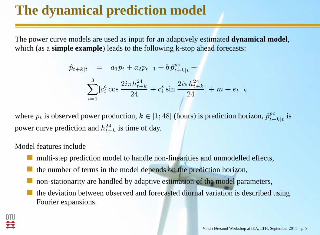
The dynamical prediction model

The power curve models are used as input for an adaptively estimateddynamical model,which (as asimple example) leads to the following k-stop ahead forecasts:

pt+k|t = a1pt + a2pt−1 + b ppc

t+k|t +

3∑

i=1

[cci cos2iπh24

t+k

24+ c

si sin

2iπh24t+k

24] +m+ et+k

wherept is observed power production,k ∈ [1; 48] (hours) is prediction horizon,ppct+k|t is

power curve prediction andh24t+k is time of day.

Model features include

multi-step prediction model to handle non-linearities andunmodelled effects,

the number of terms in the model depends on the prediction horizon,

non-stationarity are handled by adaptive estimation of themodel parameters,

the deviation between observed and forecasted diurnal variation is described usingFourier expansions.


A model for upscaling

The dynamic upscaling model for a region is defined as:

preg

t+k|t = f( wart+k|t, θ

art+k|t, k ) ploct+k|t

whereploct+k|t is a local (dynamic) power prediction within the region,war

t+k|t is forecasted regional wind speed, and

θart+k|t is forecasted regional wind direction.

The characteristics of the NWP andploc change with the prediction horizon. Hence thedependendency of prediction horizonk in the model.


Configuration Example

This configuration of WPPT is used by alarge TSO. Characteristics for the installa-tion:

A large number of wind farms andstand-alone wind turbines.

Frequent changes in the windturbine population.

Offline production data with aresolution of 15 min. is availablefor more than 99% of the windturbines in the area.

Online data for a large numberof wind farms are available. Thenumber of online wind farms in-creases quite frequently.

ModelUpscaling

predictionTotal prod.

Dynamic

Power CurveModel

Model

Offline prod.data

predictionArea prod.

NWP data

Online prod.data

predictionOnline prod.


Fluctuations of offshore wind power

Fluctuations at large offshore wind farms have a significantimpact on the control andmanagement strategies of their power output

Focus is given to the minute scale. Thus, the effects relatedto the turbulent nature ofthe wind are smoothed out

When looking at time-series of power production at Horns Rev(160MW/209MW)and Nysted (165 MW), one observes successive periods with fluctuations of largerand smaller magnitude

We aim at building models

based on historical wind powermeasures only...... but able to reproduce thisobserved behavior

this calls forregime-switchingmodels


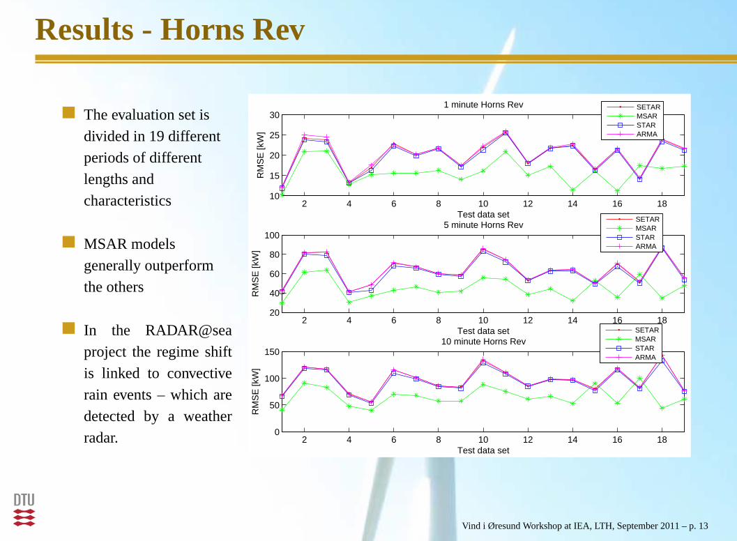
Results - Horns Rev

The evaluation set is

divided in 19 different

periods of different

lengths and

characteristics

MSAR models

generally outperform

the others

In the RADAR@sea

project the regime shift

is linked to convective

rain events – which are

detected by a weather

radar.

2 4 6 8 10 12 14 16 1810

15

20

25

30

Test data set

RM

SE

[kW

]

1 minute Horns Rev SETARMSARSTARARMA

2 4 6 8 10 12 14 16 1820

40

60

80

100

Test data set

RM

SE

[kW

]

5 minute Horns RevSETARMSARSTARARMA

2 4 6 8 10 12 14 16 180

50

100

150

Test data set

RM

SE

[kW

]

10 minute Horns RevSETARMSARSTARARMA


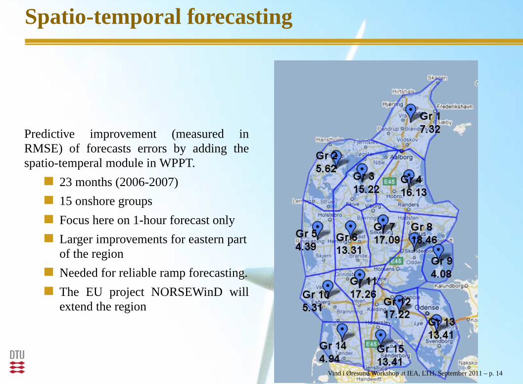
Spatio-temporal forecasting

Predictive improvement (measured inRMSE) of forecasts errors by adding thespatio-temperal module in WPPT.

23 months (2006-2007)

15 onshore groups

Focus here on 1-hour forecast only

Larger improvements for eastern partof the region

Needed for reliable ramp forecasting.

The EU project NORSEWinD willextend the region


Combined forecasting

A number of power forecasts areweighted together to form a newimproved power forecast.

These could come from parallelconfigurations of WPPT using NWPinputs fromdifferent METproviders or they could come fromother power prediction providers.

In addition to the improved perfor-mance also the robustness of the sys-tem is increased.

Met Office

DWD

DMI

WPPT

WPPT

WPPT

Comb Final

The example show results achieved for theTunø Knob wind farms using combinationsof up to 3 power forecasts.

Hours since 00Z

RM

S (

MW

)

5 10 15 20

5500

6000

6500

7000

7500

hir02.locmm5.24.loc

C.allC.hir02.loc.AND.mm5.24.loc

If too many highly correlated forecasts arecombined the performance may decreasecompared to using fewer and less corre-lated forecasts. Typically an improvementon 10-15 pct is seen by including more thanone MET provider.


Uncertainty estimation

In many applications it is crucial that a pre-diction tool delivers reliable estimates (prob-abilistc forecasts) of the expected uncertaintyof the wind power prediction.

We consider the following methods for esti-mating the uncertainty of the forecasted windpower production:

Resampling techniques.

Ensemble based - but corrected -quantiles.

Quantile regression.

Stochastic differential eqs.

The plots show raw (top) and corrected (bot-tom) uncertainty intervales based on ECMEFensembles for Tunø Knob (offshore park),29/6, 8/10, 10/10 (2003). Shown are the25%, 50%, 75%, quantiles.

Tunø Knob: Nord Pool horizons (init. 29/06/2003 12:00 (GMT), first 12h not in plan)

kW

12:00 18:00 0:00 6:00 12:00 18:00 0:00Jun 30 2003 Jul 1 2003 Jul 2 2003

020

0040

00


kW

12:00 18:00 0:00 6:00 12:00 18:00 0:00Oct 9 2003 Oct 10 2003 Oct 11 2003

020

0040

00


kW

12:00 18:00 0:00 6:00 12:00 18:00 0:00Oct 11 2003 Oct 12 2003 Oct 13 2003

020

0040

00


kW

12:00 18:00 0:00 6:00 12:00 18:00 0:00Jun 30 2003 Jul 1 2003 Jul 2 2003

020

0040

00


kW

12:00 18:00 0:00 6:00 12:00 18:00 0:00Oct 9 2003 Oct 10 2003 Oct 11 2003

020

0040

00


kW

12:00 18:00 0:00 6:00 12:00 18:00 0:00Oct 11 2003 Oct 12 2003 Oct 13 2003

020

0040

00


Quantile regression

A (additive) model for each quantile:

Q(τ) = α(τ) + f1(x1; τ) + f2(x2; τ) + . . .+ fp(xp; τ)

Q(τ) Quantile offorecast error from anexisting system.

xj Variables which influence the quantiles, e.g. the wind direction.

α(τ) Intercept to be estimated from data.

fj(·; τ) Functions to be estimated from data.

Notes on quantile regression:

Parameter estimates found by minimizing a dedicated function of the

prediction errors.

The variation of the uncertainty is (partly) explained by the independent

variables.Vind i Øresund Workshop at IEA, LTH, September 2011 – p. 17

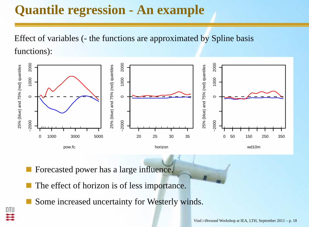
Quantile regression - An example

Effect of variables (- the functions are approximated by Spline basis

functions):

0 1000 3000 5000

−20

000

1000

2000

pow.fc

25%

(bl

ue)

and

75%

(re

d) q

uant

iles

20 25 30 35

−20

000

1000

2000

horizon

25%

(bl

ue)

and

75%

(re

d) q

uant

iles

0 50 150 250 350

−20

000

1000

2000

wd10m

25%

(bl

ue)

and

75%

(re

d) q

uant

iles

Forecasted power has a large influence.

The effect of horizon is of less importance.

Some increased uncertainty for Westerly winds.


Example: Probabilistic forecasts

5 10 15 20 25 30 35 40 450

10

20

30

40

50

60

70

80

90

100

look−ahead time [hours]

pow

er [%

of P

n]

90%80%70%60%50%40%30%20%10%pred.meas.

Notice how the confidence intervals varies ...

But the correlation in forecasts errors is not described so far.


Correlation structure of forecast errors

It is important to model theinterdependence structureof the prediction errors.

An example of interdependence covariance matrix:

5 10 15 20 25 30 35 40

5

10

15

20

25

30

35

40

horizon [h]

horiz

on[h

]

−0.2

0

0.2

0.4

0.6

0.8

1


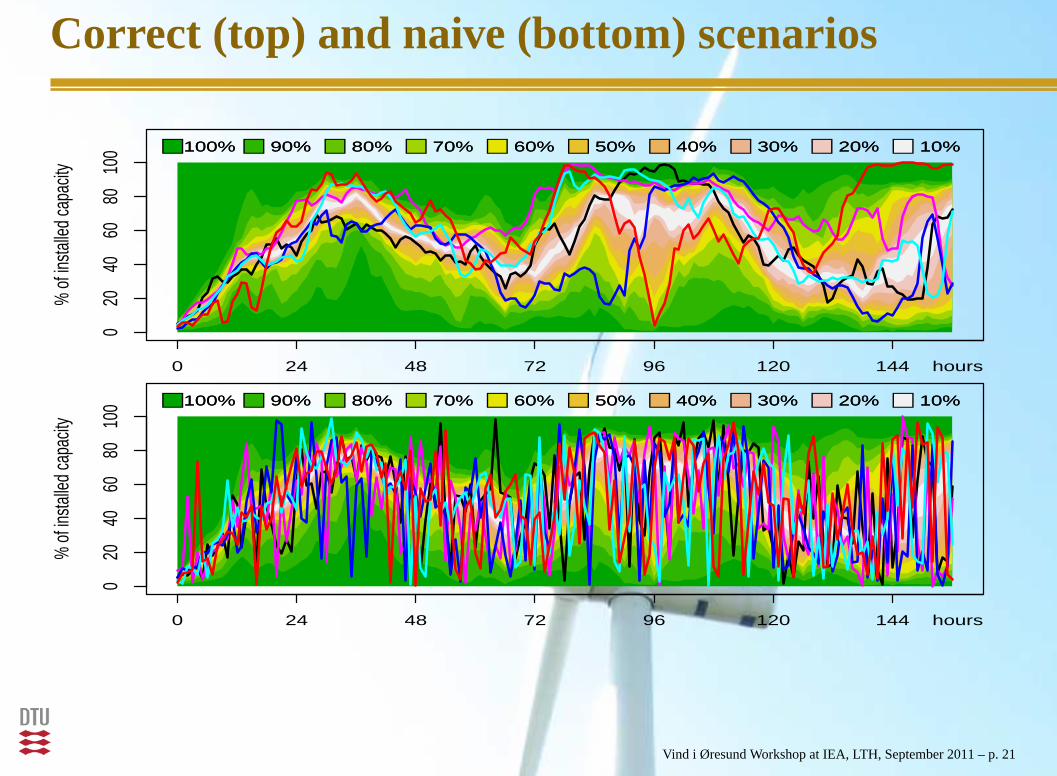
Correct (top) and naive (bottom) scenarios%

of in

stalle

d ca

pacit

y

0 24 48 72 96 120 144

020

4060

8010

0

hours

100% 90% 80% 70% 60% 50% 40% 30% 20% 10%100% 90% 80% 70% 60% 50% 40% 30% 20% 10%

% o

f insta

lled

capa

city

0 24 48 72 96 120 144

020

4060

8010

0

hours

100% 90% 80% 70% 60% 50% 40% 30% 20% 10%100% 90% 80% 70% 60% 50% 40% 30% 20% 10%


Types of forecasts required

Basic operation: Point forecasts

Operation which takes into account asymmetrical penaltieson deviations from thebid: Quantile forecasts

Stochastic optimisation taking into account start/stop costs, heat storage, and/or’implicit’ storage by allowing the hydro power production to be changed with windpower production: Scenarios respecting correctly calibrated quantiles and autocorrelation.


Wind power – asymmetrical penalties

The revenue from trading a specific hour on NordPool can be expressed as

PS × Bid +

{

PD × (Actual− Bid) if Actual > BidPU × (Actual− Bid) if Actual < Bid

PS is the spot price andPD/PU is the down/up reg. price.

The bid maximising the expected revenue is the followingquantile

E[PS ]− E[PD]

E[PU ]− E[PD]

in the conditional distribution of the future wind power production.


Wind power – asymmetrical penalties

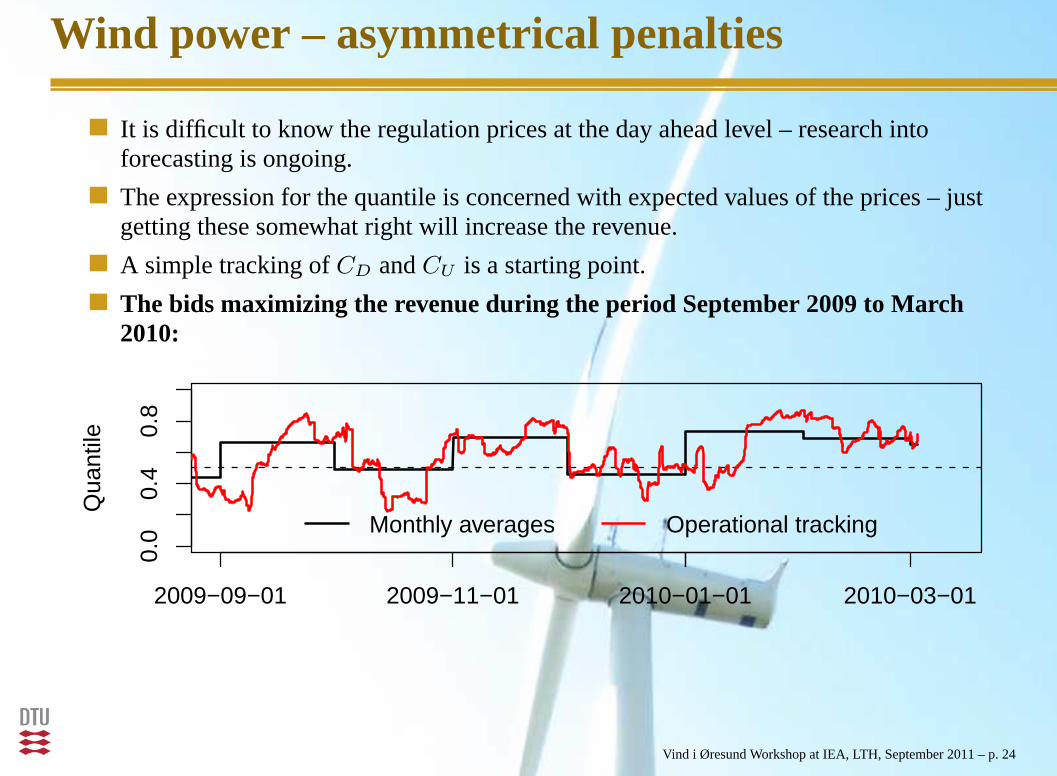
It is difficult to know the regulation prices at the day ahead level – research intoforecasting is ongoing.

The expression for the quantile is concerned with expected values of the prices – justgetting these somewhat right will increase the revenue.

A simple tracking ofCD andCU is a starting point.

The bids maximizing the revenue during the period September 2009 to March2010:

Qua

ntile

0.0

0.4

0.8

2009−09−01 2009−11−01 2010−01−01 2010−03−01

Monthly averages Operational tracking


Value of wind power forecasts

Case study: A 15 MW wind farm in the Dutch electricity market,prices andmeasurements from the entire year 2002.

From a phd thesis by Pierre Pinson (2006).

The costs are due to the imbalance penalties on the regulation market.

Value of an advanced method for point forecasting:The regulation costs arediminished by nearly 38 pct.compared to the costs of using the persistanceforecasts.

Added value of reliable uncertainties:A further decrease of regulation costs – up to39 pct.


Balancing wind by varying other production

Correct

Storage (hours of full wind prod.)

Den

sity

−10 −5 0 5 10

0.00

0.10

0.20

0.30

Naive

Storage (hours of full wind prod.)

Den

sity

−10 −5 0 5 10

0.00

0.10

0.20

0.30

(Illustrative example based on 50 day ahead scenarios as in the situation considered before)


Solar Power Forecasting

Same principles as for wind power ....

Developed for grid connected PV-systems mainly installed on rooftops

Average of output from 21 PV systems in small village (Brædstrup) in DK


Method

Based on readings from the systems and weather forecasts

Two-step method

Step One: Transformation to atmospheric transmittanceτ with statistical clear skymodel (see below). Step Two: A dynamic model (see paper).


Example of hourly forecasts


Solar Power and Electric Heating (House)


Conclusions

Some conclusions from more that 15 years of wind power forecasting:

The forecasting models must be adaptive (in order to taken changes of dust on blades,changes roughness, etc. into account).

Reliable estimates of the forecast accuracy is very important (check the reliability byeg. reliability diagrams).

Use more than a single MET provider for delivering the input to the wind powerprediction tool – this improves the accuracy with 10-15 pct.

It is advantegous if the same tool can be used for forecastingfor a single wind farm, acollection of wind farms, a state/region, and the entire country.

Use statistical methods for phase correcting the phase errors – this improves theaccuracy with up to 20 pct.

Estimates of the correlation in forecasts errors important.

Forecasts of ’cross dependencies’ between load, wind and solar power might be ofimportance. Will be tested on Bornholm in cooperation with CET at DTU Elektro.

Almost the same conclusions hold forsolar power forecasting.


Some references

H. Madsen:Time Series Analysis, Chapman and Hall, 392 pp, 2008.

H. Madsen and P. Thyregod:Introduction to General and Generalized Linear Models, Chapman

and Hall, 320 pp., 2011.

P. Pinson and H. Madsen:Forecasting Wind Power Generation: From Statistical Framework to

Practical Aspects. New book in progress - will be available 2012.

T.S. Nielsen, A. Joensen, H. Madsen, L. Landberg, G. Giebel:A New Reference for Predicting

Wind Power, Wind Energy, Vol. 1, pp. 29-34, 1999.

H.Aa. Nielsen, H. Madsen:A generalization of some classical time series tools, Computational

Statistics and Data Analysis, Vol. 37, pp. 13-31, 2001.

H. Madsen, P. Pinson, G. Kariniotakis, H.Aa. Nielsen, T.S. Nilsen: Standardizing the performance

evaluation of short-term wind prediction models, Wind Engineering, Vol. 29, pp. 475-489, 2005.

H.A. Nielsen, T.S. Nielsen, H. Madsen, S.I. Pindado, M. Jesus, M. Ignacio:Optimal Combination

of Wind Power Forecasts, Wind Energy, Vol. 10, pp. 471-482, 2007.

A. Costa, A. Crespo, J. Navarro, G. Lizcano, H. Madsen, F. Feitosa,A review on the young history

of the wind power short-term prediction, Renew. Sustain. Energy Rev., Vol. 12, pp. 1725-1744,

2008.

J.K. Møller, H. Madsen, H.Aa. Nielsen:Time Adaptive Quantile Regression, Computational

Statistics and Data Analysis, Vol. 52, pp. 1292-1303, 2008.


Some references (Cont.)

P. Bacher, H. Madsen, H.Aa. Nielsen:Online Short-term Solar Power Forecasting,Solar Energy, Vol. 83(10), pp. 1772-1783, 2009.

P. Pinson, H. Madsen:Ensemble-based probabilistic forecasting at Horns Rev. WindEnergy, Vol. 12(2), pp. 137-155 (special issue on Offshore Wind Energy), 2009.

P. Pinson, H. Madsen:Adaptive modeling and forecasting of wind power fluctuationswith Markov-switching autoregressive models. Journal of Forecasting, 2010.

C.L. Vincent, G. Giebel, P. Pinson, H. Madsen:Resolving non-stationary spectralsignals in wind speed time-series using the Hilbert-Huang transform. Journal ofApplied Meteorology and Climatology, Vol. 49(2), pp. 253-267, 2010.

P. Pinson, P. McSharry, H. Madsen.Reliability diagrams for nonparametric densityforecasts of continuous variables: accounting for serial correlation. QuarterlyJournal of the Royal Meteorological Society, Vol. 136(646), pp. 77-90, 2010.

G. Reikard, P. Pinson, J. Bidlot (2011).Forecasting ocean waves - A comparison ofECMWF wave model with time-series methods. Ocean Engineering in press.

C. Gallego, P. Pinson, H. Madsen, A. Costa, A. Cuerva (2011).Influence of localwind speed and direction on wind power dynamics - Application to offshore veryshort-term forecasting. Applied Energy, in press


Some references (Cont.)

C.L. Vincent, P. Pinson, G. Giebel (2011).Wind fluctuations over the North Sea.International Journal of Climatology, available online

J. Tastu, P. Pinson, E. Kotwa, H.Aa. Nielsen, H. Madsen (2011). Spatio-temporalanalysis and modeling of wind power forecast errors. Wind Energy 14(1), pp. 43-60

F. Thordarson, H.Aa. Nielsen, H. Madsen, P. Pinson (2010).Conditional weightedcombination of wind power forecasts. Wind Energy 13(8), pp. 751-763

P. Pinson, G. Kariniotakis (2010). Conditional predictionintervals of wind powergeneration. IEEE Transactions on Power Systems 25(4), pp. 1845-1856

P. Pinson, H.Aa. Nielsen, H. Madsen, G. Kariniotakis (2009). Skill forecasting fromensemble predictions of wind power. Applied Energy 86(7-8), pp. 1326-1334.

P. Pinson, H.Aa. Nielsen, J.K. Moeller, H. Madsen, G. Kariniotakis (2007).Nonparametric probabilistic forecasts of wind power: required properties andevaluation. Wind Energy 10(6), pp. 497-516.


forecasting wind and solar power production - iea - lund university

Documents