Forecasting the Forecasts of Others:

Implications for Asset Pricing∗

Igor Makarov† and Oleg Rytchkov‡

November 2011

Abstract

We study the properties of rational expectation equilibria (REE) in dynamic

asset pricing models with heterogeneously informed agents. We show that under

mild conditions the state space of such models in REE can be infinite dimensional.

This result indicates that the domain of analytically tractable dynamic models

with asymmetric information is severely restricted. We also demonstrate that

even though the serial correlation of returns is predominantly determined by the

dynamics of stochastic equity supply, under certain circumstances asymmetric

information can generate positive autocorrelation of returns.

Keywords: asset pricing; asymmetric information; higher order expectations; mo-

mentum

JEL classification: D82, G12, G14

∗We are very grateful to Leonid Kogan, Anna Pavlova, Steve Ross, and Jiang Wang for insightfuldiscussions and suggestions. We would like to thank the anonymous referee, the participants of sem-inars at MIT, Berkeley, Boston University, Columbia, Dartmouth College, Duke, LBS, LSE, UCSD,UBC, the participants of Frequency Domain Conclave at the University of Urbana-Champaign and2008 Meeting of the Society for Economic Dynamics for helpful comments. All remaining errors areours.†London Business School, Regent’s Park, London NW1 4SA, UK. E-mail: imakarov@london.edu‡Corresponding author: Fox School of Business and Management, Temple University, 1801 Lia-

couras Walk, 423 Alter Hall (006-01), Philadelphia, PA 19122 USA. Phone: (215) 204-4146. E-mail:rytchkov@temple.edu.

1 Introduction

This paper studies the properties of linear rational expectation equilibria in dynamic

asset pricing models with imperfectly informed agents. Since the 1970’s, the concept of

rational expectation equilibrium (REE) has become central to both macroeconomics

and finance, where agents’ expectations are of paramount importance. There is ex-

tensive evidence that in financial markets information is distributed unevenly among

different agents. As a result, prices reflect expectations of various market participants

and, therefore, are essential sources of information. To extract useful information from

prices, rational agents must disentangle the contribution of fundamentals from errors

made by other investors. Hence, it is not only the agents’ own expectations about fu-

ture payoffs that matter, but also their expectations about other agents’ expectations.

In the terminology of Townsend [45], agents forecast the forecasts of others. Trades

of each agent make the price depend on his own expectations about fundamentals, his

own mistakes, and his perception of other agents’ mistakes. This brings an additional

layer of iterated expectations. Iterating this logic forward, prices must depend on the

whole hierarchy of investors’ beliefs.1

Iterated expectations are viewed by many economists as an important feature of

financial markets and as a possible source of business cycle fluctuations. However, while

dynamic analysis has become standard in both macroeconomics and finance, formal

analysis of dynamic models with heterogeneous information has proven to be very

difficult. The reason is that in most dynamic models successive forecasts of the forecasts

of others are all different from one another. Hence, unless a recursive representation

for them is available, the dimensionality of the state space of the model grows with the

number of signals that the agents receive. As a result, both analytical and numerical

analysis of the model becomes more complicated as the number of trading periods

increases.

Although several assumptions have been identified in the literature that help pre-

serve tractability, all of them are quite restrictive. For example, a direct way to limit

the depth of higher order expectations is to assume that all private information be-

comes public after several periods (Albuquerque and Miao [3]; Brown and Jennings

[15]; Grundy and McNichols [23]; Grundy and Kim [24]; Singleton [44]). As a re-

sult, the investors’ learning problem becomes static, severely weakening the effects of

1We use the terms “hierarchy of beliefs” and “hierarchy of expectations” interchangeably. Theyare different from what is generally referred to in game theory (Biais and Bossaerts [13]; Harsanyi[25]; Mertens and Zamir [36]). In our case, agents have common knowledge of a common prior butagents’ private information is represented by infinite dimensional vectors.

1

asymmetric information on expectations, prices, and returns. Another way to make

a model tractable is to assume that agents are hierarchically informed, i.e., they can

be ranked by the amount of information they possess (Townsend [45]; Wang [49, 50]).

The simplest example is the case with two classes of agents: informed and uninformed.

Informed agents know the forecasting error of the uninformed agents and, therefore, do

not need to infer it. Thus, the series of higher order expectations collapses. Although

this information structure substantially simplifies the solution, it puts severe restric-

tions on the range of possible dynamics of agents’ expectations and their impact on

stock returns. Finally, the “forecasting the forecasts of others” problem can be avoided

if payoff-relevant fundamentals are constant over time (Amador and Weill [5]; Back,

Cao, and Willard [8]; Foster and Viswanathan [20]; He and Wang [26]) or if the number

of signals that agents receive is not less than the number of shocks in the model.

Although the simplifying assumptions are widely used in the literature, the question

as to what extent these conditions can be relaxed has not been explored. Our paper

fills this gap. We consider a dynamic asset pricing model with an infinite horizon

in which 1) each agent lacks some information available to others, 2) payoff-relevant

fundamentals evolve stochastically over time, and 3) for each agent, the dimensionality

of unobservable shocks exceeds the number of the conditioning variables. We show

that this small set of conditions can make an infinite hierarchy of iterated expectations

unavoidable and, therefore, an infinite number of state variables is required to describe

the dynamics of the economy. The establishment of this fact is a challenging problem

since even when a model does have a finite-dimensional state space, it is not obvious

how to identify those state variables in which the equilibrium dynamics have a tractable

form.

The identified conditions are quite intuitive. The first one guarantees that the

information held by other agents is relevant to each agent’s payoff. As a result, beliefs

about other agents’ beliefs affect each agent’s demand for the risky asset. The second

condition forces agents to form new sets of higher order beliefs every period. Since the

fundamentals are persistent and no agent ever becomes fully informed, all agents need

to incorporate the entire history of prices into their predictions. The third condition

makes it impossible for agents to reconstruct unknown shocks to fundamentals (or their

observational equivalents) using observable signals.

We also examine the effects of asymmetric information on asset prices. We compare

two settings with identical fundamentals but different informational structures. In the

first setting, the agents are fully informed, whereas in the second setting the informa-

2

tion is heterogeneously distributed among them. We demonstrate that the equilibrium

prices and returns are strongly affected by the allocation of information. In particular,

when there are no superiorly informed agents, the diffusion of information into prices

can be slow. Under certain circumstances, the resulting underreaction to new informa-

tion leads to a positive autocorrelation of returns. This finding shows that momentum

can be consistent with the rational expectation framework. In our model, momentum

is an equilibrium outcome of agents’ portfolio decisions. This distinguishes our expla-

nation of momentum from a number of behavioral theories as well as existing rational

theories, which show how momentum can appear in a partial equilibrium framework.

Our paper is related to the literature that explores the role of higher order expecta-

tions in asset pricing (Allen, Morris, and Shin [4]; Bacchetta and Wincoop [6]; Nimark

[38]; Woodford [52]). In particular, Allen, Morris, and Shin [4] emphasize the failure

of the law of iterated expectations for average expectations. As a consequence, under

asymmetric information agents tend to underreact to private information, biasing the

price towards the public signal and producing a drift in the price process. Their in-

tuition is challenged by Banerjee, Kaniel, and Kremer [9], who argue that asymmetric

information alone cannot generate price drift and suggest “differences in opinions”,

i.e., disagreements about higher order beliefs, as a possible source of momentum. In

this paper, we show that the serial correlation of returns is determined by an interplay

between two different effects. On the one hand, slow diffusion of information increases

persistence of returns. On the other hand, the stochastic asset supply contributes to

negative return autocorrelation (this effect is pure in the full information case). Hence,

the serial correlation of returns depends on the relative strength of the two effects. In

general, neither a slow diffusion of information nor a breakdown of the law of iterated

expectations is sufficient to generate momentum. Nevertheless, we demonstrate that

the information dispersion can have a qualitative effect on the serial correlation of

returns if the effect of stochastic supply is sufficiently suppressed.

To analyze the model, we transform it from the time domain to the frequency

domain. First developed by Futia [21], this technique has found many applications

(Bernhardt, Seiler, and Taub [12]; Kasa [33]; Kasa, Walker, and Whiteman [34]; Walker

[48]). Similar to our paper, Bernhardt, Seiler, and Taub [12] consider a dynamic

model with stochastic fundamentals and heterogeneously informed agents. However,

their model features a finite number of risk neutral investors who can individually

affect prices and, hence, behave strategically. Thus, their work focuses on the effects

of competition on information revelation, trading strategies, and price behavior. In

3

contrast, in our model investors are risk averse and behave competitively, as they are

unable to move the price individually. Their trading behavior is determined not by a

strategic revelation of information, but by risk considerations.

The rest of the paper is organized as follows. Section 2 describes the model. In

Section 3, we prove that a simple version of our model has the “forecasting the forecasts

of others” problem and that its dynamics cannot be described in terms of a finite

number of state variables. In Section 4 we examine the impact of information dispersion

on serial correlations of returns and discuss the dynamics of higher order expectations.

In particular, we demonstrate that heterogeneous information accompanied by evolving

fundamentals can produce momentum. Section 5 concludes. Technical details are

presented in Appendices A and B.

2 Setup

This section presents our main setup, which will be used for analysis of the “forecasting

the forecasts” problem and the serial correlation of returns. The setup includes most

of the essential elements common to dynamic asset pricing models with asymmetric

information.

The uncertainty in the model is described by a complete probability space (X ,F , µ)

equipped with a filtration Ft. Time is discrete. There are two assets in the model:

a riskless asset and a risky asset (“stock”). The riskless asset is assumed to be in

infinitely elastic supply at a constant gross rate of return R. Each share of the stock

pays a dividend Dt at time t ∈ Z. Following Grossman and Stiglitz [22], we assume

that the total amount of risky equity available to rational agents is Θt and attribute

the time variation in Θt to noise trading. This assumption prevents prices from being

fully revealing in an equilibrium, and thus gives a scope for asymmetric information.

We assume that the processes Dt and Θt are stationary, adapted to the filtration Ft,and jointly Gaussian. The normality assumption is standard for asset pricing models

with asymmetric information. It ensures the linearity of conditional expectations and,

therefore, makes models tractable.

There is a continuum of competitive investors who are assumed to be uniformly

distributed on a unit interval [0, 1]. All investors have an exponential utility function

with the same constant risk-aversion parameter α and derive utility from their accu-

mulated wealth in the next period. The assumption of one-period investment horizon

is common in the asset pricing literature with asymmetric information (e.g., Allen,

4

Morris, and Shin [4], Bacchetta and Wincoop [7], Singleton [44], Walker [48]). In this

case, investors have no hedging component in their demand for the risky asset. In our

setup, this is especially advantageous since the calculation of the hedging demand in

an economy with an infinite number of state variables presents a considerable technical

challenge. Sidestepping this problem allows us to preserve tractability of the model.

Let F it ⊆ Ft be an information set of investor i generated by some stationary signals.

It is natural to assume that F it always includes the current price of the risky asset Pt

and its current dividend Dt as well as all their past realizations. In addition, investors

may receive some information about noise trading (past, current, or future) or future

dividends, and this information may vary across investors. Hence, each investor i at

time t solves the following portfolio problem:

maxxi

t

E[−e−αW it+1|F it ] (1)

subject to the budget constraint

W it+1 = xitQt+1 +W i

tR, (2)

where Qt+1 = Pt+1 + Dt+1 − RPt is the stock’s excess return at time t + 1 and W it is

accumulated wealth. It is well-known that the solution to this problem is

xit = ωiE[Qt+1|F it ], (3)

where ωi = (αVar[Qt+1|F it ])−1 is a constant due to the normality and stationarity

assumptions.

The rational expectation equilibrium in the model is characterized by (i) the price

process Pt, which is assumed to be adapted to the filtration Ft and (ii) the trading

strategies xit, which solve the optimization problem in Eq. (1) and in each period t

satisfy the market clearing condition∫ 1

0

xitdi = Θt.

The market clearing condition allows us to represent the equilibrium price in terms

of expectations of future fundamentals Dt and Θt. It is convenient to define the

weighted average expectation operator Et[ · ], which summarizes the expectations

5

of individual investors:

Et[ · ] = Ω

∫ 1

0

ωiE[ · |F it ]di, Ω =

[∫ 1

0

ωidi

]−1

. (4)

Using this operator, the market clearing condition can be succinctly rewritten as

ΩΘt = Et[Qt+1]. (5)

Since the equilibrium price Pt is observed by all investors, combining the definition of

excess returns and Eq. (5) yields an explicit equation for the price process:

Pt = −λΘt + βEt[Dt+1 + Pt+1], (6)

where we introduce β = R−1 and λ = βΩ for the ease of notation. Iterating Eq. (6)

forward and imposing the standard no-bubble condition limt→∞ βtPt = 0, we obtain

another representation for the equilibrium price:

Pt = −λΘt +∞∑s=0

βs+1Et...Et+s (Dt+s+1 − λΘt+s+1) . (7)

Eq. (7) represents the price as a sum of iterated average expectations of future realiza-

tions of processes Dt and Θt. In general, the information sets of investors are different,

so the law of iterated expectations for the weighted average expectation operator Et[ · ]does not hold. As a result, investors must forecast not only future values of Dt and Θt

but also expectations of other agents, and, therefore, non-trivial higher order expec-

tations arise. Eq. (7) reveals the potential source of the “forecasting the forecasts of

others” problem. Indeed, the current price Pt depends on agents’ future expectations,

which, in turn, depend on future prices (recall that Pt+s is in the information set of all

investors and is used for conditioning in Et+s[ · ]). Hence, to find the equilibrium in the

model it is necessary to solve a fixed point problem for the entire sequence of prices.

As we demonstrate below, it is a very complicated problem unless the information sets

F it have a very special structure.

3 Information Dispersion and Dynamics of Prices

In this section, we rigorously prove that the information dispersion can produce the

“forecasting the forecasts of others” problem, i.e., that the dynamics of the model

6

cannot be described in terms of a finite number of state variables. Instead of working

with the very general model described in the previous section, we consider its special

version. On the one hand, it allows us to keep the proof as short as possible. On

the other hand, even in its reduced form the model preserves all elements which are

necessary for the existence of the “forecasting the forecasts of others” problem.

First, we assume that Dt ≡ 0, i.e., the price of the asset is solely determined by

the risk premium required by investors for liquidity provision to noise traders. The

main benefit of setting dividends to zero comes from the reduction in the number of

observables available to investors, and the resulting simplification of investors filtering

problem. Second, we assume that the process Θt consists of a persistent component Vt

and a transitory component bεΘt :

Θt = Vt + bεΘt , (8)

where b is a non-zero constant. In its turn, Vt also contains two components following

AR(1) processes with the same persistence parameter a:

Vt = V 1t + V 2

t ,

V jt+1 = aV j

t + εjt+1, j = 1, 2.

The innovations ε1t , ε

2t , and εΘ

t are assumed to be jointly independent and normally

distributed with zero mean and unit variance.

There are two types of investors labeled by j = 1, 2. Each type populates a subset

of a unit interval with a measure of 1/2. All investors observe the price process Pt.

The informational structure of the model is determined by what investors of each type

know about the persistent components V 1t and V 2

t .

As a benchmark, we consider a full information case in which the information sets

of investors are

F1t = F2

t = Pτ , V 1τ , V

2τ : τ ≤ t.

It means that all investors observe both V 1t and V 2

t , i.e., have all relevant informa-

tion about future fundamentals available at time t. Since the information sets of

investors are identical, the law of iterated expectations holds for average expectations:

EtEt+1...Et+sVt+s+1 = EtVt+s+1 = as+1Vt. At the same time, EtεΘt+s = 0 for s > 0.

Hence, the infinite sum in Eq. (7) can be computed explicitly and we obtain a simple

7

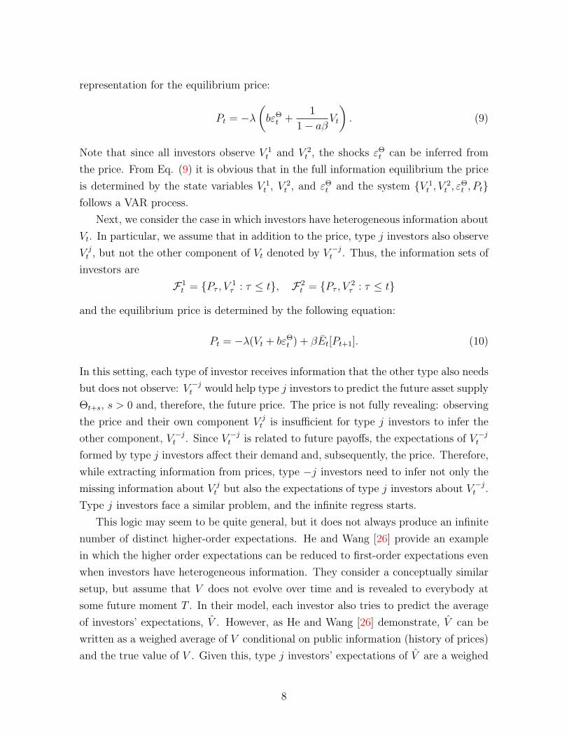
representation for the equilibrium price:

Pt = −λ(bεΘt +

1

1− aβVt

). (9)

Note that since all investors observe V 1t and V 2

t , the shocks εΘt can be inferred from

the price. From Eq. (9) it is obvious that in the full information equilibrium the price

is determined by the state variables V 1t , V 2

t , and εΘt and the system V 1

t , V2t , ε

Θt , Pt

follows a VAR process.

Next, we consider the case in which investors have heterogeneous information about

Vt. In particular, we assume that in addition to the price, type j investors also observe

V jt , but not the other component of Vt denoted by V −jt . Thus, the information sets of

investors are

F1t = Pτ , V 1

τ : τ ≤ t, F2t = Pτ , V 2

τ : τ ≤ t

and the equilibrium price is determined by the following equation:

Pt = −λ(Vt + bεΘt ) + βEt[Pt+1]. (10)

In this setting, each type of investor receives information that the other type also needs

but does not observe: V −jt would help type j investors to predict the future asset supply

Θt+s, s > 0 and, therefore, the future price. The price is not fully revealing: observing

the price and their own component V jt is insufficient for type j investors to infer the

other component, V −jt . Since V −jt is related to future payoffs, the expectations of V −jt

formed by type j investors affect their demand and, subsequently, the price. Therefore,

while extracting information from prices, type −j investors need to infer not only the

missing information about V jt but also the expectations of type j investors about V −jt .

Type j investors face a similar problem, and the infinite regress starts.

This logic may seem to be quite general, but it does not always produce an infinite

number of distinct higher-order expectations. He and Wang [26] provide an example

in which the higher order expectations can be reduced to first-order expectations even

when investors have heterogeneous information. They consider a conceptually similar

setup, but assume that V does not evolve over time and is revealed to everybody at

some future moment T . In their model, each investor also tries to predict the average

of investors’ expectations, V . However, as He and Wang [26] demonstrate, V can be

written as a weighed average of V conditional on public information (history of prices)

and the true value of V . Given this, type j investors’ expectations of V are a weighed

8

average of their first-order expectations, conditional on past prices and on their past

private signals. Since V is constant, the aggregation of investors’ private signals also

produces V . Therefore, the second (and higher) order expectations of V can also be

expressed in terms of a weighted average of V conditional on past prices and the true

value of V .

This logic breaks down when Vt evolves stochastically over time. In this case,

investors form expectations not only about the value of Vt at a particular moment,

but also about all previous realizations of Vt. New information arriving in each period

changes the way investors use their past signals; they need to reestimate the whole

path of their expectations. This means that investors have to track an infinite number

of state variables and that the logic described above does not hold.

It is important to know whether a model has a finite or infinite number of state

variables because the two cases call for different solution techniques. In the former

case, the major problem is to find the appropriate state space variables. In the latter,

the search for a finite set of state variables that can capture the dynamics is doomed,

and the solution of such models presents a greater challenge.

Until now, the “forecasting the forecasts of others” problem was defined relatively

loosely. To lay the groundwork for its rigorous treatment, we introduce the concept of

Markovian dynamics.

Definition. Let Xt be a multivariate stationary adapted random process. We

say that Xt admits Markovian dynamics if there exists a collection of n <∞ adapted

random processes Yt = Y it , i = 1 . . . n, such that the joint process (Xt, Yt) is a Markov

process:

Prob(Xt ≤ x, Yt ≤ y|Xτ , Yτ : τ ≤ t− 1

)= Prob

(Xt ≤ x, Yt ≤ y|Xt−1, Yt−1

).

While it is obvious that any Markov process admits Markovian dynamics, the op-

posite is not true. The following example helps to clarify the difference.

Let εt, t ∈ Z be i.i.d. standard normal random variables and consider an MA(1)

process Xt such that Xt = εt−θεt−1 where θ is a constant. Xt is not a Markov process,

or even an n-Markov process: Prob (Xt|Xτ : τ ≤ t− 1) 6= Prob (Xt|Xt−1, . . . , Xt−n)

for any n. However, Xt can be easily extended to a Markov process by augmenting it

with εt.

Applying the concept of Markovian dynamics to our model with heterogeneous

information, we get the main result of the paper.

9

Theorem 1 Suppose that type j investors’ information set is given by F jt = Pτ , V jτ :

τ ≤ t, j = 1, 2. Then, in the linear equilibrium the system V 1, V 2, εΘ, P does not

admit Markovian dynamics.

Proof. See Appendix A.

The main idea of the proof is to use the following result from the theory of stationary

Gaussian processes: if a multivariate process admits Markovian dynamics, then it can

be described by a set of rational functions in the frequency domain. We start the proof

assuming that the equilibrium admits Markovian dynamics, so the price function in the

frequency domain is rational. The proof then consists of showing that if we work only

with rational functions, it is impossible to simultaneously satisfy the market clearing

condition and solve the filtering problem of each agent. This contradiction proves that

the equilibrium does not admit Markovian dynamics.

To the best of our knowledge, we are the first who rigorously demonstrate that the

infinite regress problem does indeed arise naturally in a rational expectation equilibrium

of dynamic models with heterogeneous information. Ironically, Townsend [45] who

inspired the study of the infinite regress problem and coined the term “forecasting the

forecasts of others”, actually developed a model without the infinite regress problem

(Kasa [33]; Pearlman and Sargent [39]; Sargent [43]). This illustrates how challenging

it could be even to diagnose the presence of the “forecasting the forecasts of others”

problem in a particular setting. Theorem 1 suggests a set of typical conditions for its

existence. If each agent lacks some information available to other agents, fundamentals

evolve stochastically over time, and dimensionality of unknown shocks exceeds that of

conditioning variables then an infinite hierarchy of iterated expectations arises. Almost

all of these conditions are also necessary. For example, as demonstrated by He and

Wang [26], if the fundamentals are constant, then it is possible to avoid the “forecasting

the forecasts of others” problem.

The infinite regress problem can be viewed as a rational justification for technical

analysis. To a statistician who has only public information, the dynamics of prices

might appear to be quite simple. However, for an investor who has additional pri-

vate information the joint dynamics of prices and his private signals can become very

complicated. We show that even with a very simple specification of the fundamentals,

asymmetric information makes equilibrium dynamics highly non-trivial. To be as effi-

cient as possible, agents use the entire history of prices in their predictions. Moreover,

as Theorem 1 demonstrates, investors cannot summarize the available information with

a finite number of state variables. In other words, investors’ strategies become path-

10

dependant, often in a convoluted way. This suggests that in financial markets where

the asymmetry of information is common, the entire history of prices may be very

important to investors and have a profound effect on their actions.

A model with an infinite number of state variables calls for an appropriate solu-

tion technique. In Appendix B we describe one of the ways to solve the model. Since

an analytical solution is not feasible, we construct a numerical approximation to the

equilibrium. This approach allows us to evaluate the effects of various information dis-

tributions on prices and returns and explore the dynamics of higher order expectations.

4 Higher order expectations and autocorrelations

of returns

In this section we explore the link between asymmetric information and autocorrelation

of returns. A non-zero autocorrelation implies the predictability of next period returns

by current returns and the existence of potentially profitable trading opportunities.

In the asset pricing literature, positive serial correlations are often associated with

momentum whereas negative serial correlations imply a reversal in stock returns.2

Consider again the general model presented in Section 2. We first observe that the

autocorrelation structure of returns in rational expectation equilibria is determined to

a large extent by the assumed process for the stochastic supply of equity Θt. The

market clearing condition in Eq. (5) implies that the unconditional autocovariance

of excess returns Qt is solely determined by the contemporaneous covariance between

excess returns and the supply of equity:

Cov(Qt+1, Qt) = ΩCov(Qt,Θt). (11)

Our derivation of Eq. (11) explicitly assumes that investors are myopic and have

no hedging demand. However, Eq. (11) would also hold in a more general setting.

If investors had a CARA utility function over the long horizon, any hedging demand

resulting solely from the asymmetric information would be a linear function of investors’

forecast errors. Since by definition, the forecast errors are orthogonal to the public

information set including past prices and dividends, the covariance of the hedging

demand with past returns would be zero and Eq. (11) would still hold. For example,

2The empirical literature on momentum is very large. See Jegadeesh and Titman [30] for the initialcontribution and Jegadeesh and Titman [31] for a review.

11

Eq. (11) is valid in the setups of He and Wang [26] and Wang [49].

Thus to get further insights, we have to make some specific assumptions about

Θt. The next theorem characterizes the autocorrelation of returns when the stochastic

supply of equity follows an AR(1) process.

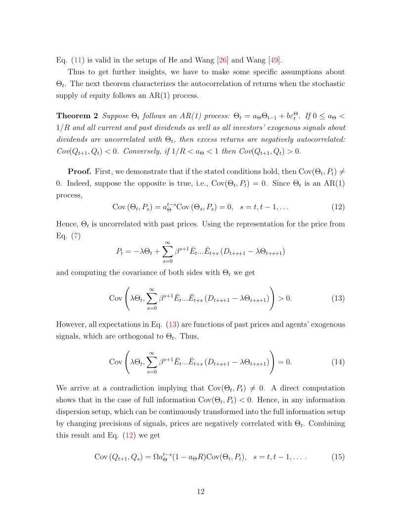
Theorem 2 Suppose Θt follows an AR(1) process: Θt = aΘΘt−1 + bεΘt . If 0 ≤ aΘ <

1/R and all current and past dividends as well as all investors’ exogenous signals about

dividends are uncorrelated with Θt, then excess returns are negatively autocorrelated:

Cov(Qt+1, Qt) < 0. Conversely, if 1/R < aΘ < 1 then Cov(Qt+1, Qt) > 0.

Proof. First, we demonstrate that if the stated conditions hold, then Cov(Θt, Pt) 6=0. Indeed, suppose the opposite is true, i.e., Cov(Θt, Pt) = 0. Since Θt is an AR(1)

process,

Cov (Θt, Ps) = at−sΘ Cov (Θs, Ps) = 0, s = t, t− 1, . . . (12)

Hence, Θt is uncorrelated with past prices. Using the representation for the price from

Eq. (7)

Pt = −λΘt +∞∑s=0

βs+1Et...Et+s (Dt+s+1 − λΘt+s+1)

and computing the covariance of both sides with Θt we get

Cov

(λΘt,

∞∑s=0

βs+1Et...Et+s (Dt+s+1 − λΘt+s+1)

)> 0. (13)

However, all expectations in Eq. (13) are functions of past prices and agents’ exogenous

signals, which are orthogonal to Θt. Thus,

Cov

(λΘt,

∞∑s=0

βs+1Et...Et+s (Dt+s+1 − λΘt+s+1)

)= 0. (14)

We arrive at a contradiction implying that Cov(Θt, Pt) 6= 0. A direct computation

shows that in the case of full information Cov(Θt, Pt) < 0. Hence, in any information

dispersion setup, which can be continuously transformed into the full information setup

by changing precisions of signals, prices are negatively correlated with Θt. Combining

this result and Eq. (12) we get

Cov (Qt+1, Qs) = Ωat−sΘ (1− aΘR)Cov(Θt, Pt), s = t, t− 1, . . . . (15)

12

Hence, the autocorrelations of returns are negative when Θt follows an AR(1) process

with 0 ≤ aΘ ≤ 1/R.

It is interesting to note that Theorem 2 seemingly contradicts the findings of Brown

and Jennings [15] who obtain a positive autocorrelation of returns in a rational expec-

tation equilibrium with persistent noise trading. The two results can be reconciled

by realizing that while our model is stationary and has an infinite horizon, the model

of Brown and Jennings (1989) has only two periods. In their case, several artificial

features such as deterministic changes in conditional variance of returns or the impact

of boundary conditions can have substantial effect on autocorrelations of returns. In

a stationary model, we eliminate these obscuring effects and show that asymmetric

information alone cannot generate momentum when the demand from noise traders

follows an AR(1) process.

The impossibility of generating momentum with AR(1) traders emphasizes that

slow diffusion of information or breakdown of the law of iterated expectations are not

sufficient conditions for momentum. In our model, the autocorrelation of returns is

determined by the interplay of two different effects. On the one hand, the downward

sloping demand curve of rational investors together with the mean reverting stochastic

supply produce a negative autocorrelation of returns (this effect is easiest to see in

the full information case). On the other hand, since investors are heterogeneously

informed, the diffusion of information into prices may be slow, and this increases the

autocorrelation of returns. Hence, the statistical properties of returns depend on which

effect is stronger. When the demand from noise traders follows an AR(1) process, Eq.

(15) shows that the latter effect is always stronger.

The weakness of the information effect may not be specific to the case with the

AR(1) equity supply. A distinctive property of the AR(1) process is that today’s

expectations of future realizations decline monotonically (in absolute terms) with the

horizon. As a result, the supply of equity and prices tend to revert. Thus, it is

reasonable to expect that for all processes with as > as+1, where as = E(εΘt−sΘt) the

effect of heterogeneous information is weaker than the effect of mean reverting equity

supply.

We would like to emphasize that our conclusion crucially depends on the speci-

fication of equity supply as an exogenous process. If instead we assume that it is

endogenously determined (e.g., as a function of past returns), the autocorrelation of

returns may become positive. To illustrate this point, suppose that the time varia-

tion in equity supply is produced by feedback traders (in the terminology of De Long,

13

Shleifer, Summers, and Waldmann [17]), whose demand for the stock is proportional

to the last period return. Since Eq. (11) still holds, we immediately obtain that in this

case, the first-order autocorrelation of returns is positive.

Although the asymmetry of information cannot change the sign of return autocor-

relations when Θt follows an AR(1) process, the situation is different if the exogenous

equity supply follows a more general process. As an example, we consider the case

when Θt is an AR(2) process defined as Θt = (a1Θ + a2Θ)Θt−1 − a1Θa2ΘΘt−2 + bεΘt .

To demonstrate the effect of asymmetric information on the dynamics of returns, we

choose the parameters a1Θ and a2Θ so that the serial correlation of returns is negative

in the full information case. Specifically, we set a1Θ = 0.55 and a2Θ = 0.8. The innova-

tions εΘt are i.i.d. with the standard normal distribution and b = 0.2. Also, we assume

that the dividend Dt consists of three components: Dt = D1t + D2

t + bDεDt . The first

two components follow AR(1) processes:

Dit = aDi

t−1 + biεit, i = 1, 2.

The shocks ε1t , ε

2t , and εDt are also i.i.d. with the standard normal distribution. In the

numerical example we set a = 0.8, b1 = b2 = 0.7, and bD = 0.9. For simplicity, the

risk-free rate is set to be zero, so R = 1.3 As in Section 3, we assume that there are two

types of investors. Type i investors perfectly observe Dit, so F it = Ps, Di

st−∞. This

model contains all elements required for the existence of the “forecasting the forecasts

of others” problem and it is very likely that it does not admit a Markovian dynamics.

Hence, the statistical properties of returns can be explored only numerically. The

detailed description of our computations is relegated to Appendix B.

Table I reports serial correlations of returns in models with the full information and

heterogeneous information. For the chosen set of parameters, returns are negatively

autocorrelated when investors are fully informed. However, the autocorrelation is pos-

itive for the same fundamentals in the heterogeneous information case. It means that

if stochastic supply follows an AR(2) process, momentum can exist in the rational ex-

pectation equilibrium. Intuitively, in this case the negative autocorrelation of returns

produced by mean reversion of the equity supply is relatively weak, and the informa-

tion dispersion effect is strong enough to change the sign of the autocorrelation from

negative to positive. However, the magnitudes of autocorrelations are rather small,

3Although our results are obtained for this specific combination of parameters, we also examinedalternative models with other parameters and found that our qualitative conclusions are not drivenby this particular choice.

14

Full Info Heterogeneous Info

Corr(Qt+1, Qt) -0.0002 0.0001

Std(∆t) 0 1.6574

Corr(∆t,∆t−1) — 0.6217

Corr(Θt,∆t) — -0.3930

Corr(εDt ,∆t) — 0.6121

Table I: Statistics of returns Qt and the informational component of the price ∆t inthe full information and heterogeneous information equilibria.

and our setup falls short of explaining momentum quantitatively.

To better understand the impact of asymmetric information on dynamics of returns,

it is convenient to decompose the price from Eq. (7) into a component that is deter-

mined solely by the fundamentals and a correction term ∆t produced by heterogenous

information. Denoting the expectation operator with respect to full information at

time t as Et, we obtain the following representation for the price:

Pt = −λΘt +∞∑s=0

βs+1Et(Dt+s+1 − λΘt+s+1)︸ ︷︷ ︸full information component

+∆t, (16)

where

∆t =∞∑s=0

βs+1(Et...Et+s − Et)(Dt+s+1 − λΘt+s+1). (17)

The term ∆t represents the effect of asymmetric information. If investors are fully

informed, the chain of iterated average expectations collapses and the information term

disappears: ∆t = 0.4 In the heterogeneous information setup, due to the violation of the

law of iterated expectations for average expectations Et, all higher order expectations

are different. Therefore, ∆t is non-trivial and has two effects. On the one hand, it

produces a gap between the price of the firm and its fundamental value. On the other

hand, it affects the dynamics and statistical properties of prices and returns.

To illustrate the impact of ∆t, we compute its volatility and autocorrelation as well

as its correlations with Θt and εDt . The results are presented in Table I. First, note

that in the heterogeneous information case the standard deviation of ∆t is quite high

and represents a substantial part of the price variation. Hence, higher order expecta-

tions play an important role in the price formation. Second, Table I shows that ∆t

4In the full information solution, the constant λ is also different.

15

εit εDt εΘt

Figure 1: Impulse response of ∆t to the shocks εit, εDt , and εΘ

t .

is highly persistent under heterogeneous information: its autocorrelation coefficient is

0.62. Intuitively, when investors are heterogeneously informed, they all make forecast-

ing errors. The errors made by one type of investors depend not only on fundamentals

but also on the errors made by the other type. In the absence of fully informed arbi-

trageurs, errors are persistent since it takes several periods for investors to realize that

they made mistakes and to correct them.

This intuition is also illustrated by the impulse response functions of ∆t presented

in Figure 1. Indeed, ∆t has high negative loadings on εit and εΘt and positive loadings

on εDt . When there is a shock to one of the persistent components Dit, the investors who

observe Dit increase their demand and drive the price upward. Investors who cannot

observe Dit partially attribute the price increase to a negative shock to the aggregate

asset supply Θt and underreact relative to the full information case. Hence, the price

is lower and ∆t is negative. However, observing subsequent realizations of prices and

dividends, uninformed investors infer that is was a shock to Dit and also increase their

demand, driving the price up towards its full information level. A similar logic explains

negative loadings of ∆t on εΘt .

A positive reaction of ∆t to εDt is also quite natural. When εDt is positive, investors

observe a higher dividend. Unable to disentangle the persistent components D1t and

D2t from εDt , they partially attribute the increase in dividends to positive ε1

t or ε2t . As

a result, investors value the asset more and drive the price up. As time passes and new

realizations of dividends become available, they learn their mistake and ∆t decreases.

The described relations between ∆t and the fundamental shocks also explain the

correlations reported in Table I. Indeed, ∆t is negatively correlated with Θt and pos-

itively with εDt . Given that εDt are i.i.d., the latter correlation is a direct consequence

of the positive impulse response of ∆t to εDt . The former correlation is less straightfor-

ward, since Θt is a persistent process. However, if learning is relatively fast, then the

16

sign of the correlation Corr(Θt,∆t) is mostly determined by the correlation between ∆t

and εΘt , which is negative.

Overall, when investors are heterogeneously informed, the information may pene-

trate into prices quite slowly. As a result, the sign of the serial correlation of returns

may change, and returns can be positively autocorrelated in the equilibrium, an out-

come that points towards a rational explanation for momentum. This mechanism is

distinct from behavioral stories, which attribute momentum to under-reaction or de-

layed over-reaction caused by cognitive biases (Barberis, Shleifer, and Vishny [10];

Daniel, Hirshleifer, and Subrahmanyam [16]; Hong and Stein [27]). It is also quite

different from existing rational explanations, which are based on partial equilibrium

models (Berk, Green, and Naik [11]; Johnson [32]; Sagi and Seasholes [42]).

5 Concluding remarks

In this paper, we develop a dynamic asset pricing model with heterogeneous infor-

mation and study the structure of its rational expectation equilibrium. The model

demonstrates the mechanics of the “forecasting the forecasts of others” problem and

shows that an infinite hierarchy of higher order expectations naturally arises in such

a setting. Moreover, we give a formal proof that under very mild conditions it is

impossible to describe the dynamics of the economy using a finite number of state

variables.

Due to the complexity of the problem, we make several simplifying assumptions.

However, it is reasonable to believe that the intuition behind our conclusions is also

valid in more realistic models. First, while our model considers only one firm, it would

be interesting to analyze a similar setup with multiple firms. Such an analysis would

extend existing static models (Admati [1]; Easley and O’Hara [19]; Hughes, Liu, and

Liu [28]) and grant new insights into the effect of information distribution on cross-

correlations of prices and returns.5 Next, in this paper we consider myopic investors

with no hedging demand. This significantly simplifies the analysis; otherwise we would

have to solve a dynamic program with an infinite dimensional state space. The impact

of hedging could be non-trivial and requires further investigation.

In our model, agents are exogenously endowed with their information; they can

neither buy new information, nor release their own if they find this exchange profitable.

It might be interesting to relax this assumption and introduce a market for information.

5See Biais, Bossaerts, and Spatt [14] and Watanabe [51] for some results in the dynamic setting.

17

Such extensions have been studied in a static setting by Admati and Pfleiderer [2],

Verrecchia [46], and others, but the dynamic properties of the market for information

have not been thoroughly explored6.

Although our analysis pertains mostly to asset pricing, it may provide new in-

sights into various aspects of the “ forecasting the forecasts of others” problem and

iterated expectations in general. The intuition behind our results is also relevant to

other fields. For example, higher order expectations naturally arise in several different

macroeconomic settings (Lorenzoni [35]; Rondina [41]; Woodford [52]), in the analysis

of exchange rate dynamics (Bacchetta and Wincoop [6]), in models of industrial or-

ganization where firms have to extract information about unknown cost structure of

their competitors (Vives [47]). Adapting our approach to the analysis of higher order

expectations in these fields may be a fruitful direction for future research.

Appendix A

Proof of Theorem 1

The main idea of the proof is to transform the analysis from the time domain into the

frequency domain. Therefore, before proceeding with the proof, we introduce some

notations and state several relevant results from the theory of stochastic processes.

Time and Frequency Domains

Consider an infinite sequence of three-dimensional random vectors εt = (ε1t , ε

2t , ε

Θt ),

t ∈ Z. The random variables ε1t , ε

2t , ε

Θt are independent, normal, and have zero mean

and unit variance. We say that the process Xt is a stationary regular Gaussian process

adapted to the filtration generated by εt if it can be written as

Xt =∞∑k=0

xkε′t−k,

where the three-dimensional constant coefficients xk are square summable:

∞∑k=0

xkx′k <∞.

6See Naik [37] for analysis of a monopolistic information market in a dynamic framework.

18

The set of such processes is a pre-Hilbert space H with an inner product of vectors

Xt =∞∑k=0

xkε′t−k and Yt =

∞∑k=0

ykε′t−k

defined as

E[XtYt] =∞∑k=0

xky′k.

Thus, two processes are orthogonal if they are uncorrelated. The infinite sequence of

coefficients xk, k = 0, 1, ... can be viewed as a representation of the process in the time

domain.

Instead of working with an infinite number of coefficients, it is often convenient to

introduce the frequency domain representation. We will say that a three-dimensional

function X(z) is a z-representation of the process Xt if

X(z) =∞∑k=0

xkzk.

The components of X(z) are well-defined analytical functions in the unit disk D0 = z :

|z| < 1 in the complex plane C. The corresponding inner product takes the following

form:

E[XtYt] =1

2πi

∮X(z)Y (z−1)′

dz

z, (A1)

where the integral is taken in the complex plane along the contour |z| = 1. Eq. (A1)

creates a bridge between the correlation structure of random variables and the location

of singularities of their z -representation functions.

Let L be a shift operator defined as Lεt = εt−1. Using its z-representation we can

write the process Xt as:

Xt = X(L)ε′t. (A2)

From (A2) it is clear that zX(z) corresponds to the lagged process Xt−1.

Markovian Dynamics in the Frequency Domain

The concept of Markovian dynamics introduced in Section 3 can be concisely defined in

the frequency domain representation. We rely on the following result from the theory

of stationary Gaussian processes (see Doob [18] for the original results and Ibragimov

and Rozanov [29] for a textbook treatment).

19

Theorem 3 Let Xt be a regular stationary Gaussian process with discrete time defined

on a complete probability space (Ω,F , µ). The process Xt admits Markovian dynamics

with a finite number of Gaussian state variables if and only if its z-representation is a

rational function of z.

The following examples serve to illustrate the theorem. They show that several well-

known processes admitting Markovian dynamics have indeed rational z-representation.

Example 1. Let Xt be i.i.d. over time: Xt = εt. In this case, x0 = 1 and xk = 0, for

k = 1, 2.... Thus X(z) ≡ 1.

Example 2. Let Xt be an AR(1) process: Xt = aXt−1 + εt. In this case, xk = ak, for

k = 0, 1, .... Thus X(z) = (1− az)−1.

Example 3. Let Xt be an MA(1) process: Xt = εt − θεt−1. In this case, x0 = 1,

x1 = −θ, xk = 0, for k = 2, 3, .... Thus X(z) = 1− θz.

Main Part of the Proof

We showed in Section 3 that the equilibrium price function satisfies the following equa-

tion:

Pt = −λ(Vt + bεΘt ) + βEt[Pt+1], (A3)

where 0 < β < 1. Recall that λ = βΩ, where

Ω−1 =1

2α

(1

Var[Qt+1|F1t ]

+1

Var[Qt+1|F2t ]

).

Hence, λ is endogenous, i.e., it is determined in the equilibrium along with the process

for Pt. However, to prove that the equilibrium does not admit Markovian dynamics it

is sufficient to prove that Eq. (A3) has no solution that admits Markovian dynamics

for any arbitrary λ 6= 0 treated as an exogenous constant. This is the path we follow

below.

Because we focus on a stationary linear equilibrium, we assume that the price Pt is

a stationary regular adapted Gaussian process represented as

Pt =∞∑k=0

fkε1t−k +

∞∑k=0

fkε2t−k + b

∞∑k=0

fΘk ε

Θt−k, (A4)

20

or in the frequency domain:

Pt = f(L)ε1t + f(L)ε2

t + bfΘ(L)εΘt , f(z) =

∞∑k=0

fkzk, fΘ(z) =

∞∑k=0

fΘk z

k. (A5)

We prove Theorem 1 in several steps. First, we use the frequency domain representation

of the equilibrium price and reformulate the equilibrium conditions in terms of the func-

tions f(z) and fΘ(z). Second, we assume that the system of processes V 1, V 2, εΘ, Padmits Markovian dynamics. In this case, according to Theorem 3 f(z) and fΘ(z)

must be rational. Finally, we demonstrate that rational f(z) and fΘ(z) cannot satisfy

the equilibrium conditions. This contradiction proves Theorem 1.

Step 1. It is convenient to start with the filtering problem of each agent. Eq.

(A3) implies that each type i investor must find the best estimate of Pt+1 given his

information set F it = V is , Pst−∞. Since some components of Pt are known to investor

i, the information set F it = V is , Pst−∞ is identical to F it = V i

s , Zist−∞, where

Zit = f(L)ε−it + bfΘ(L)εΘ

t . (A6)

The filtering problem is equivalent to finding a projector G such that

E[Zit+1|F it ] = G(L)Zi

t . (A7)

By definition, Zit+1 −G(L)Zi

t is orthogonal to all Zis, s ≤ t:

E[(Zit+1 −G(L)Zi

t

)Zis] = 0. (A8)

Calculating expectations we get

E[Zit+1Z

is] =

1

2πi

∮ 1

z2f(z)

1

zt−sf(z−1) + b2 1

z2fΘ(z)

1

zt−sfΘ(z−1)

dz,

E[G(L)ZitZ

is] =

1

2πi

∮ 1

zG(z)f(z)

1

zt−sf(z−1) +b2 1

zG(z)fΘ(z)

1

zt−sfΘ(z−1)

dz.

After collecting all terms, the orthogonality condition (A8) takes the form

1

2πi

∮1

zkU(z)dz = 0, k = 1, 2, . . . , (A9)

21

where the function U(z) is

U(z) =

(1

z−G(z)

)(f(z)f(z−1) + b2fΘ(z)fΘ(z−1)

). (A10)

Using Eq. (A3), we get a set of equations for f(z) and fΘ(z):

− 2λ

1− az− 2f(z) + β

f(z)− f(0)

z+ βG(z)f(z) = 0, (A11)

(1− βG(z))fΘ(z) + λ = 0. (A12)

For further convenience we introduce the function

g(z) =1

λ(βG(z)− 1). (A13)

Using this definition, Eqs. (A11), (A12), and (A10) can be rewritten as

f(z) =βf(0)− z(aβf(0)− 2λ)

(1− az)(β − z + λzg(z)), (A14)

fΘ(z) =1

g(z), (A15)

U(z) =β − z − λzg(z)

βz

(f(z)f(z−1) + b2fΘ(z)fΘ(z−1)

). (A16)

Step 2. Assume that the system of processes V 1, V 2, εΘ, P admits Markovian

dynamics. Then, the projection of Pt+1 on F it also admits Markovian dynamics. By

Theorem 3, its z-representation G(z) must be rational. Hence, from Eqs. (A13), (A14),

and (A15), the functions g(z), f(z), and fΘ(z) should be rational as well. Given the

rationality of G(z), f(z), and fΘ(z), Eq. (A9) implies that U(z) is analytic in C except

for a finite number of poles within the unit circle D0 = z : |z| < 1 and U(∞) = 0. To

prove that our model has non-Markovian dynamics, it is sufficient to show that there

exist no rational functions f(z), fΘ(z), g(z) and U(z) such that 1) f(z), fΘ(z), and

g(z) are analytic inside the unit circle and U(z) is analytic outside the unit circle; 2)

U(∞) = 0; 3) Eqs. (A14), (A15), and (A16) hold.

Step 3. Inspired by the structure of Eqs. (A14) and (A16), we introduce the

22

function H(z) such that

g(z) = (β − z + λzg(z))H(z)/β (A17)

Remarkably, all the equilibrium functions f(z), fΘ(z), g(z), and U(z) can easily be

rewritten in terms of the function H(z) and all analyticity conditions on the equilibrium

functions can be translated into conditions on the function H(z). Thus, the question

of the existence of the equilibrium with Markovian dynamics reduces to the question

of the existence of a function H(z) satisfying a set of conditions.

From Eq. (A17) the function g(z) is

g(z) =(β − z)H(z)

β − λzH(z). (A18)

Recall that β is the implicit discount factor in Eq. (A3) satisfying 0 < β < 1. Since

fΘ(z) = 1/g(z), we have

fΘ(z) =β − λzH(z)

(β − z)H(z). (A19)

Substitution of Eq. (A18) into Eq. (A14) gives

f(z) =βf(0)− z(aβf(0)− 2λ)

β(1− az)(β − z)(β − λzH(z)). (A20)

If aβf(0)− 2λ 6= 0 we can define z1 as

z1 =βf(0)

aβf(0)− 2λ

and rewrite the function f(z) in the following form:

f(z) = (aβf(0)− 2λ)z1 − z

β(1− az)(β − z)(β − λzH(z)). (A21)

The structure of the function U(z) depends on whether aβf(0)− 2λ 6= 0 (z1 is finite)

or aβf(0) − 2λ = 0 (z1 = ∞). In the first case, using Eqs. (A15), (A18), and (A21)

23

U(z) can be rewritten as

U(z) =

(1

zH(z)− 2λ

β

)[

(aβf(0)− 2λ)2(z − z1)(z−1 − z1)

β2(1− az)(1− az−1)H(z)H(z−1) + b2

]1

g(z−1). (A22)

Since g(z) does not have poles in D0 (and, consequently, g(z−1) does not have poles in

D∞), the analyticity of U(z) in D∞ implies the analyticity of U g(z) = U(z)g(z−1) in

D∞. Hence,

U g(z) =

(1

zH(z)− 2λ

β

)[(aβf(0)− 2λ)2(z − z1)(z−1 − z1)

β2(1− az)(1− az−1)H(z)H(z−1) + b2

](A23)

must be analytical in D∞. In a special case aβf(0)−2λ = 0 (i.e., z1 =∞), the function

U g(z) takes a simpler form:

U g(z) =

(1

zH(z)− 2λ

β

)[4λ2

a2β2(1− az)(1− az−1)H(z)H(z−1) + b2

]. (A24)

First, consider the general case with aβf(0) − 2λ 6= 0 (finite z1). The following

lemma describes the properties of H(z).

Lemma 1 The function H(z) can satisfy the equilibrium conditions only if

1. H(z) is rational;

2. H (β) = 1λ

;

3. H(z) may have poles only at z1 or z−11 , where z1 6= 0, and the order of poles

cannot exceed 1;

4. H(z) may have zeros only at a−1 and z1 ∈ D∞, and the order of zeros cannot

exceed 1.

Proof.

Statement 1 follows from the assumed rationality of fΘ(z) and Eq. (A19).

Since fΘ(z) must be analytic in D0, the pole z = β in Eq. (A19) must cancel, and

this implies 1− λH(β) = 0. This is Statement 2.

Also, the analyticity of fΘ(z) implies that H(z) 6= 0 for z ∈ D0. For the rest of the

statements we need the conditions on functions f(z) and U(z).

24

By assumption, f(z) is analytic in D0. The pole β in Eq. (A21) disappears since

1−λH(β) = 0 (Statement 2), but H(z) may have first-order poles at z = 0 and z = z1

(if z1 6= 0) or a second-order pole at z = 0 (if z1 = 0), which potentially may not violate

the analyticity of f(z). An existence of a pole at z = 0 of any order would mean that

the function g(z) has a pole at z = 0 (this follows from Eq. (A18)) in contradiction

to its analyticity in D0. Hence, in D0 the function H(z) may have only the pole

z = z1 6= 0, and the order of this pole cannot exceed 1. In D∞ the possible poles are

determined by the analyticity of U(z). Indeed, a pole in H(z) must be canceled by a

zero in(z − z1)(z−1 − z1)

(1− az)(1− az−1)H(z−1).

Clearly, it can be 1) either z1 or z−11 depending on whether z1 is in D∞ or D0, or 2) a

zero of H(z−1). The second option contradicts H(z) 6= 0 for z ∈ D0 and we arrive at

Statement 3.

Since H(z) 6= 0 for z ∈ D0, H(z) may have zeros in D∞ only. However, a zero of

H(z) may produce a pole in U(z) (the term b2/(zH(z)) in Eq. (A23)) which would

contradict its analyticity in D∞. This happens unless the pole is canceled by a pole in

another term in Eq. (A23). Such a pole can be either a−1 or a pole of H(z−1). Since

for z−1 ∈ D0 the function H(z−1) may have a first-order pole in z1 only, Statement 4

follows.

Lemma 1 implies that if z1 = 0 (i.e., f(0) = 0), then the function H(z) must have

a linear form H(z) = A(z − a−1)k, where A is a non-zero constant and k is either 0

or 1. In the latter case, Eq. (A23) and the condition U g(∞) = 0 yields the following

equation for A:4λ2A2

a2β2+ b2 = 0. (A25)

Obviously, it cannot be satisfied. If H(z) is a constant (k = 0) then the condition

U g(∞) = 0 reduces to b2 = 0 which is also violated. Thus, we have showed that if

z1 = 0 then the equilibrium does not admit Markovian dynamics.

Consider now the case of z1 6= 0. According to Lemma 1, if z1 6= 0 the function

H(z) must have the following representation:

H(z) =A(z − z1)k1(z − a−1)k2

(z − z1)p1(z − z−11 )p2

,

where k1, k2, p1, and p2 can be either 0 or 1, k1 6= 1 if p1 = 1, and A is a constant.

Let the number of poles in H(z) be P and the number of zeros be K: K = k1 + k2,

25

P = p1 + p2. The condition U g(∞) = 0 imposes some restrictions on K and P ,

summarized in Lemma 2.

Lemma 2 If z1 6= 0, then either P = K or P = K + 1.

Proof. Since z1 6= 0, we have

(z − z1)(z−1 − z1)

(1− az)(1− az−1)−→ z1

a6= 0 as z −→∞.

If P < K we have H(z) → ∞ as z → ∞. Because H(0) = const 6= 0 (Lemma 1) the

function U g(z) from Eq. (A23) is not finite at infinity: U g(z)→∞. If P > K+ 1 then

zH(z)→ 0 as z →∞ and again U g(z)→∞.

The asymptotic condition U g(∞) = 0 also imposes restrictions on the constant A.

If z1 6= 0 and P = K, then the condition U g(∞) = 0 implies that

f(0)2 zk1−p1+p2−11

ak2+1A2 + b2 = 0. (A26)

If P = K + 1 the condition U g(∞) = 0 yields

1

A− 2λ

β= 0. (A27)

Note that the constant A is also fixed by Lemma 1, which states that H(β) = 1/λ.

Thus,

A =1

λ

(β − z1)p1(β − z−11 )p2

(β − z1)k1(β − a−1)k2. (A28)

Combining the implications of Lemmas 1 and 2, it is convenient to summarize all

possible cases in one table:

poles

zeros ∅ z1 z−11 z1, z−1

1

∅ (1) (2) (3) X

z1 X X (4) X

a−1 X (5) (6) (7)

z1, a−1 X X X X

Note that according to Lemma 1 in all cases involving z1 we assume that z1 6= 0. In

the rest of the proof, we show that none of the seven cases can realize.

26

Case 1: k1 = k2 = p1 = p2 = 0, i.e., H(z) = A.

In this case, Eqs. (A26) and (A28) reduce to

f(0)2

az1

A2 + b2 = 0, A =1

λ. (A29)

The analyticity of the function U g(z) in D∞ is achieved only if the pole z = a−1 cancels

out. This can happen for three reasons:

1. z1 = a;

2. z1 = a−1;

3. −λβ

+ a2A

= 0.

If z1 = a, Eq. (A29) reduces to

f(0)2

a2A2 + b2 = 0,

which obviously does not have solutions. Similarly, if z1 = a−1, Eq. (A29) yields

f(0)2A2 + b2 = 0,

which also cannot be satisfied. In the third case, the exogenous parameters of the

model should satisfy a very specific condition

aβ = 2, (A30)

which cannot be fulfilled since 0 < a < 1, 0 < β < 1.

Case 2: k1 = k2 = p2 = 0, p1 = 1, i.e., H(z) = A/(z − z1).

In this case, Eqs. (A27) and (A28) reduce to

A =β

2λ, A =

β − z1

λ.

Combining these equations we get z1 = β/2. The pole z = a−1 in the function U g(z)

disappears only if

−λβ

+1− az1

2A= 0.

Substituting for A and z1 in this equation yields aβ = 0, which cannot be satisfied.

27

Case 3: k1 = k2 = p1 = 0, p2 = 1, i.e., H(z) = A/(z − z−11 ).

Similar to case 2, Eqs. (A27) and (A28) reduce to

A =β

2λ, A =

β − z−11

λ.

Combining these equations we get z−11 = β/2. The pole z = a−1 in the function U g(z)

disappears only if

−λβ

+1− a

z1

2A= 0.

After simple algebraic manipulations we again get aβ = 0, which cannot be satisfied.

Case 4: k2 = p1 = 0, k1 = p2 = 1, i.e., H(z) = A(z − z1)/(z − z−11 ).

Since H(z) cannot have zeros in D0 (Lemma 1), z1 ∈ D∞. However, in this case a

pole of U g(z) in D∞ arises, and it can be canceled only if z1 = a−1. Eq. (A26) reduces

to

f(0)2A2

a2+ b2 = 0 (A31)

and cannot be satisfied.

Case 5: k1 = p2 = 0, k2 = p1 = 1, i.e., H(z) = A(z − a−1)/(z − z1), z1 6= a−1.

In this case Eq. (A26) reduces to

f(0)2

a2z21

A2 + b2 = 0

which cannot be satisfied.

Case 6: k1 = p1 = 0, k2 = p2 = 1, i.e., H(z) = A(z − a−1)/(z − z−11 ), z1 6= a.

Similar to case 5, Eq. (A26) reduces to

f(0)2

a2A2 + b2 = 0 (A32)

which cannot be satisfied.

Case 7: k1 = 0, k2 = p1 = p2 = 1, i.e., H(z) = A(z − a−1)/((z − z1)(z − z−11 )),

z1 6= a, z1 6= a−1.

Note that in this case the function U g(z) always has a pole in D∞ (z1 or z−11 ), which

does not cancel out. This violates the analyticity of U g(z) in D∞ and precludes case

7.

28

Finally, consider a special case in which aβf(0)− 2λ = 0 (it can be understood as

z1 =∞). Lemma 3 below is an analog of Lemma 1; it describes the conditions on the

function H(z).

Lemma 3 The function H(z) can satisfy the equilibrium conditions only if

1. H(z) is rational;

2. H (β) = 1λ

;

3. H(z) is analytic in the whole complex plane C;

4. H(z) may have a zero at a−1 only, and the order of this zero cannot exceed 1.

Proof.

Similar to Lemma 1, Statements 1 and 2 follow from the required conditions on

fΘ(z) and g(z). Also, the analyticity of fΘ(z) implies that H(z) 6= 0 for z ∈ D0. Next,

Eq. (A20) can be rewritten as

f(z) =2λ

aβ(1− az)(β − z)(β − λzH(z)). (A33)

By assumption, f(z) is analytic in D0. The pole z0 in Eq. (A33) disappears since

1 − λH(β) = 0 (Statement 2), but H(z) may have a first-order pole at z = 0 which

potentially may not violate the analyticity of f(z). However, an existence of a pole at

z = 0 of any order would mean that the function g(z) has a pole at z = 0 (this follows

from Eq. (A18)) in contradiction to its analyticity in D0. Hence, the function H(z)

is analytic in D0. In D∞ the possible poles are determined by the analyticity of U(z).

Indeed, from Eq. (A24) a pole in H(z) must be canceled by a zero in

1

(1− az)(1− az−1)H(z−1).

Clearly, it can be only a zero of H(z−1). However, such zeros don’t exist since H(z) 6= 0

for z ∈ D0. Thus, we arrive at Statement 3.

Since H(z) 6= 0 for z ∈ D0, H(z) may have zeros only in D∞. However, a zero of

H(z) may produce a pole in U(z) (the term b2/(zH(z)) in Eq. (A24)) which would

contradict its analyticity in D∞. This happens unless the pole is canceled by a pole in

another term in Eq. (A24). Such a pole can be either a−1 or a pole of H(z−1). Since

for z−1 ∈ D0 the function H(z−1) is analytic, Statement 4 follows.

29

Taken together, the statements of Lemma 3 effectively imply that either H(z) = A

or H(z) = A(1 − az), where A is a non-zero constant. However, in the first case Eq.

(A24) yields U g(∞) = −2λb2/β. This is a contradiction to the condition U g(∞) = 0.

In the second case, the condition U g(∞) = 0 implies

4λ2

a2β2A2 + b2 = 0,

which also cannot be satisfied. This completes the proof of the theorem.

Appendix B

In this appendix, we describe the numerical method of computing approximate solu-

tions to the version of our model presented in Section 4. To construct this approxima-

tion, we assume that all information is revealed to all investors after k periods, so the

information set of investor i is F it = Pτ , Diτ : τ ≤ t; D−iτ ,Θτ : τ ≤ t− k. As before,

−i denotes an investor type other than type i. When Θt follows an AR(2) process, it

is convenient to characterize the state of the economy Ψt in terms of the current values

of D1t , D

2t , Θt, Θt−1, and by their k lags:

Ψt = (ψt, ψt−1, . . . , ψt−k)′, where ψτ = (D1

τ , D2τ ,Θτ ,Θτ−1)′.

The demand of type i investors is

X it = ωiE[Qt+1|F it ] = ωi(aD

it −RPt + E[aD−it + Pt+1|F it ]).

We look for the equilibrium price process as a linear function of state variables: Pt =

PΨt, where P is a (1 × 4(k + 1)) constant matrix. In the matrix form, the dynamics

of ψt are:

ψt+1 = aψψt + εψt+1,

where

aψ =

a 0 0 0

0 a 0 0

0 0 −(a1Θ + a2Θ) a1Θa2Θ

0 0 1 0

, εψt =

ε1t

ε2t

εΘt

0

, Var(εψt ) =

b2V 0 0 0

0 b2V 0 0

0 0 b2 0

0 0 0 0

.

30

Consequently, the dynamics of Ψt can be described as:

Ψt+1 = AΨΨt +BΨεψt+1, where AΨ =

aψ 0 . . . 0 0

I4 0 . . . 0 0

0 I4 . . . 0 0...

.... . .

......

0 0 . . . I4 0

, BΨ =

I4

0

0...

0

.

Here I4 is a four-dimensional unit matrix. In terms of the state variables Ψt the demand

can be rewritten as

X it = ωi(aD

it −RPt + E[aD−it + PAΨΨt|F it ]).

Introducing (1× 4(k + 1)) constant matrices D1 = (1, 0, 0, . . . , 0), D2 = (0, 1, 0, . . . , 0)

and D = (1, 1, 0, . . . , 0), we get

X it = −ωiRPt + ωi(aD + PAΨ)E[Ψt|F it ].

Thus, we have to calculate E[Ψt|F it ]. Denoting the observations of agent i at time

t as yit = (Pt, Dit)′, we can gather all his relevant observations into one vector Y i

t =

(yit, yit−1, . . . , yt−k+1, ψt−k). It is also convenient to introduce a set of Pτ , τ = t−k+1 . . . t

in order to separate the informative part of the price:

Pt = Pt,

Pt−1 = Pt−1 − P kψt−k−1,

. . .

Pt−k+1 = Pt−k+1 − P 2ψt−k−1 − . . .− P kψt−2k.

Now we can put all observations in a matrix form:

Y it = H iΨt, where H i =

hi

hiJ

hiJ2

...

hiJk

O3×3k I3

, J =

0 I4 0 . . . 0

0 0 I4 . . . 0...

......

. . ....

0 0 0 . . . I4

0 0 0 . . . 0

, hi =

(P

V i

)

31

We use the following well-known fact: if (Ψ, Y ) are jointly normal with zero mean,

then

E[Ψ|Y ] = β′Y, where β = Var(Y )−1E(YΨ′),

Var[Ψ|Y ] = Var(Ψ)− E(YΨ′)′Var(Y )−1E(YΨ′).

In our particular case we have:

Var(Y it ) = H iVar(Ψt)H

i′.

E(Y iΨ′) = H iVar(Ψt)

From the dynamic equation for Ψt we find that

Var(Ψt) = AΨVar(Ψt)A′

Ψ +BΨVar(εψt )B′

Ψ.

Iteration of this equation yields

Var(Ψt) =∞∑l=0

AlΨBΨVar(εψt )B′

ΨAlΨ

′.

Thus, the demand of agent i is

X it = −ωiRPt + ωi(aD + PAΨ)Var(Ψt)H

i′(H iVar(Ψt)Hi′)−1H iΨt.

Imposing the market clearing condition and taking into account that there is an equal

number of agents of each type we get

−RPt +1

2(aD + PAΨ)Var(Ψt)H

1′(H1Var(Ψt)H1′)−1H1Ψt

+1

2(aD + PAΨ)Var(Ψt)H

2′(H2Var(Ψt)H2′)−1H2Ψt = ΩΘΨt,

where Θ = (0, 0, 1, 0, 0, . . . , 0) and Ω is defined in Section 2. Rearranging the terms we

get:

Pt =1

2β(aD + PAΨ)Var(Ψt)×

×[H1′(H1Var(Ψt)H

1′)−1H1 +H2′(H2Var(Ψt)H2′)−1H2

]Ψt − λΘΨt,

32

where λ = Ω/R. Comparing this equation with the price representation Pt = PΨt, we

get a matrix equation:

P =1

2β(aD + PAΨ)Var(Ψt)×

×(H1′(H1Var(Ψt)H

1′)−1H1 +H2′(H2Var(Ψt)H2′)−1H2

)− λΘ. (B1)

As a result, when all information is revealed after k lags the equilibrium condition

transforms into a system of non-linear equations (B1) that determines P . A numerical

solution to these equations gives us an approximation to the REE with heterogeneous

information.

References

[1] A. R. Admati, A noisy rational expectations equilibrium for multi-asset securities

markets, Econometrica 53 (1985) 629–657.

[2] A. R. Admati, P. Pfleiderer, A monopolistic market for information, J. Econ.

Theory 39 (1986) 400–438.

[3] R. Albuquerque, J. Miao, Advance information and asset prices, Unpublished

manuscript, 2010.

[4] F. Allen, S. Morris, H. S. Shin, Beauty contests and iterated expectations in asset

markets, Rev. Finan. Stud. 19 (2006) 719–752.

[5] M. Amador, P. Weill, Learning from private and public observations of others’

actions, J. Econ. Theory (2011) forthcoming.

[6] Ph. Bacchetta, E. van Wincoop, Can information heterogeneity explain the ex-

change rate determination puzzle? Amer. Econ. Rev. 96 (2006) 552–576.

[7] Ph. Bacchetta, E. van Wincoop, Higher order expectations in asset pricing, J.

Money, Credit, Banking 40 (2008) 837–866.

[8] K. Back, C. H. Cao, G. A. Willard, Imperfect competition among informed traders,

J. Finance 55 (2000) 2117–2155.

[9] S. Banerjee, R. Kaniel, and I. Kremer, Price drift as an outcome of differences in

higher order beliefs, Rev. Finan. Stud. 22 (2009) 3707–3734.

33

[10] N. Barberis, A. Shleifer, R. Vishny, A model of investor sentiment, J. Finan. Econ.

49 (1998) 307–343.

[11] J. B. Berk, R. C. Green, V. Naik, Optimal investment, growth options, and secu-

rity returns, J. Finance 54 (1999) 1553–1607.

[12] D. Bernhardt, P. Seiler, B. Taub, Speculative dynamics, Econ. Theory 44 (2010)

1–52.

[13] B. Biais, P. Bossaerts, Asset prices and trading volume in a beauty contest, Rev.

Econ. Stud. 65 (1998) 307–340.

[14] B. Biais, P. Bossaerts, and C. Spatt, Equilibrium asset pricing and portfolio choice

under asymmetric information, Rev. Finan. Stud. 23 (2010) 1503–1543.

[15] D. P. Brown, R. H. Jennings, On technical analysis, Rev. Finan. Stud. 2 (1989)

527–552.

[16] K. Daniel, D. Hirshleifer, A. Subrahmanyam, Investor psychology and security

market under-and overreaction, J. Finance 53 (1998) 1839–1885.

[17] J. B. De Long, A. Shleifer, L. H. Summers, R. J. Waldmann, Positive feedback

investment strategies and destabilizing rational speculation, J. Finance 45 (1990)

379–395.

[18] J. L. Doob, The elementary Gaussian processes, Ann. Math. Stat. 15 (1944) 229–

282.

[19] D. Easley, M. O’Hara, Information and the cost of capital, J. Finance 59 (2004)

1553–1583.

[20] F. D. Foster, S. Viswanathan, Strategic trading when agents forecast the forecasts

of others, J. Finance 51 (1996) 1437–1477.

[21] C. A. Futia, Rational expectations in stationary linear models, Econometrica 49

(1981) 171–192.

[22] S. J. Grossman, J. E. Stiglitz, On the impossibility of informationally efficient

markets, Amer. Econ. Rev. 70 (1980) 393–408.

[23] B. D. Grundy, M. McNichols, Trade and revelation of information through prices

and direct disclosure, Rev. Finan. Stud. 2 (1989) 495–526.

34

[24] B. D. Grundy, Y. Kim, Stock market volatility in a heterogenous information

economy, J. Finan. Quant. Anal. 37 (2002) 1–27.

[25] J. C. Harsanyi, Games with incomplete information played by ’Bayesian’ players,

I: The basic model, Manage. Science 14 (1967) 159–182.

[26] H. He, J. Wang, Differential information and dynamic behavior of stock trading

volume, Rev. Finan. Stud. 8 (1995) 919–972.

[27] H. Hong, J. Stein, A unified theory of underreaction, momentum trading, and

overreaction in asset markets, J. Finance 54 (1999) 2143–2184.

[28] J. Hughes, J. Liu, J. Liu, Information asymmetry, diversification, and cost of

capital, Acc. Rev. 82 (2005) 705–729.

[29] I.A. Ibragimov, Y.A. Rozanov, Gaussian Random Processes, Springer-Verlag,

1978.

[30] N. Jegadeesh, S. Titman, Returns to buying winners and selling losers: Implica-

tions for stock market efficiency, J. Finance 48 (1993) 65–91.

[31] N. Jegadeesh, S. Titman, Momentum, in R. H. Thaler (editor), Advances in Be-

havioral Finance, Vol. 2, Princeton University Press, 2005.

[32] T. C. Johnson, Rational momentum effects, J. Finance 57 (2002) 585–607.

[33] K. Kasa, Forecasting the forecasts of others in the frequency domain, Rev. Econ.

Dynam. 3 (2000) 726–756.

[34] K. Kasa, T. B. Walker, C. H. Whiteman, Heterogeneous beliefs and tests of present

value models, Unpublished manuscript, 2010.

[35] G. Lorenzoni, A theory of demand shocks, Amer. Econ. Rev. 99 (2009) 2050–2084.

[36] J.-F. Mertens, S. Zamir, Formulations of Bayesian analysis for games with incom-

plete information, Int. J. Game Theory 14 (1985) 1–29.

[37] N. Y. Naik, Multi-period information markets, J. Econ. Dynam. Control 21 (1997)

1229–1258.

[38] K. Nimark, Dynamic higher order expectations, Unpublished manuscript, 2011.

35

[39] J. G. Pearlman, T. J. Sargent, Knowing the forecasts of others, Rev. Econ. Dynam.

8 (2005) 480–497.

[40] W. Qiu, J. Wang, Asset pricing under heterogeneous information, Unpublished

manuscript, 2009.

[41] G. Rondina, Incomplete information and informative pricing, Unpublished

manuscript, 2008.

[42] J. Sagi, M. Seasholes, Firm-specific attributes and the cross-section of momentum,

J. Finan. Econ. 84 (2007) 389–434.

[43] T. J. Sargent, Equilibrium with signal extraction from endogenous variables, J.

Econ. Dynam. Control 15 (1991) 245–273.

[44] K. J. Singleton, Asset prices in a time-series model with disparately informed, com-

petitive traders, in Barnett, W. A. and Singleton , K. J. (eds.), New Approaches

to Monetary Economics, Proceedings of the Second International Symposium in

Economic Theory and Econometrics, Cambridge University Press, 1987.

[45] R. M. Townsend, Forecasting the forecasts of others, J. Polit. Economy 91 (1983)

546–588.

[46] R. E. Verrecchia, Information acquisition in a noisy rational expectations economy,

Econometrica 50 (1982) 1415–1430.

[47] X. Vives, Aggregation of information in large Cournot markets, Econometrica 56

(1988) 851–876.

[48] T. Walker, How equilibrium prices reveal information in time series models with

disparately informed, competitive traders, J. Econ. Theory 137 (2007) 512–537.

[49] J. Wang, A model of intertemporal asset prices under asymmetric information,

Rev. Econ. Stud. 60 (1993) 249–282.

[50] J. Wang, A model of competitive stock trading volume, J. Polit. Economy 102

(1994) 127–168.

[51] M. Watanabe, Price volatility and investor behavior in an overlapping generations

model with information asymmetry, J. Finance 63 (2008) 229–272.

36

[52] M. Woodford, Imperfect common knowledge and the effects of monetary policy,

in P. Aghion, R. Frydman, J. Stiglitz, and M. Woodford (eds.), Knowledge, Infor-

mation, and Expectations in Modern Macroeconomics: In Honor of Edmund S.

Phelps, Princeton University Press, 2002.

37