forecasting the dynamics of a coastal fishery species ... · forecasting the dynamics of a coastal...

Hare et al. – Climate forecasts for a coastal fishery 1

Forecasting the dynamics of a coastal fishery species using a coupled climate-population model

Jonathan A. Hare 1†, Michael A. Alexander 2, Michael J. Fogarty 3, Erik H. Williams4, James D. Scott 2

1 NOAA NMFS Northeast Fisheries Science Center, Narragansett Laboratory, 28 Tarzwell Drive, Narragansett, RI, 02818, USA.

2 NOAA/Earth System Research Laboratory Physical Sciences Division 325 Broadway Boulder, CO, 80305, USA.

3 NOAA NMFS Northeast Fisheries Science Center, Woods Hole Laboratory, 166 Water Street, Woods Hole, MA, 02543, USA.

4 NOAA NMFS Southeast Fisheries Science Center, 101 Pivers Island Road, Beaufort, NC, 28516, USA.

† corresponding author - NOAA NMFS Northeast Fisheries Science Center, Narragansett Laboratory, 28 Tarzwell Drive, Narragansett, RI, 02818, USA. phone – (401) 782-3295; FAX – (401) 782-3201; email – [email protected]

Submitted to Ecological Applications as an Article


Abstract 1

Marine fisheries management strives to maintain sustainable populations while allowing 2

exploitation. However, well-intentioned management plans may not meet this balance as 3

most do not include the effect of climate change. Ocean temperatures are expected to 4

increase through the 21st century, which will have far-reaching and complex impacts on 5

marine fisheries. To begin to quantify these impacts for one coastal fishery along the east 6

coast of the United States, we develop a coupled climate-population model for Atlantic 7

croaker (Micropogonias undulatus). The model is based on a mechanistic hypothesis: 8

recruitment is determined by temperature-driven, overwinter mortality of juveniles in 9

their estuarine habitats. Temperature forecasts were obtained from 14 General Circulation 10

Models simulating three CO2 emission scenarios. An ensemble-based approach was used 11

in which a multimodel average was calculated for a given CO2 emission scenario to 12

forecast the response of the population. The coupled model indicates that both 13

exploitation and climate change significantly affect abundance and distribution of 14

Atlantic croaker. At current levels of fishing, the average (2010-2100) spawning biomass 15

of the population is forecast to increase by 60-100%. Similarly, the center of the 16

population is forecast to shift 50-100 km northwards. A yield analysis, which is used to 17

calculate benchmarks for fishery management, indicates that the maximum sustainable 18

yield will increase by 30-100%. Our results demonstrate that climate effects on fisheries 19

must be identified, understood, and incorporated into the scientific advice provided to 20

managers if optimum exploitation is to be achieved in a changing climate. 21

22


KEYWORDS: Climate change, fishery management, population dynamics, abundance, 23

distribution, environmental effects, Atlantic croaker 24

25

Introduction 26

Overexploitation results in dramatic declines in marine population abundance and 27

affects overall marine ecosystem structure. Fishing is often the dominant source of post-28

juvenile mortality for exploited species, causing direct reductions in population 29

abundance (Myers et al. 1997, Christensen et al. 2003). Most fishing practices truncate 30

the age and size distribution through increased mortality and size-selectivity, which 31

potentially reduces reproductive potential of the population because larger females may 32

produce more and higher quality offspring (O'Farrell and Botsford 2006, Scott et al. 33

2006). Fishing also impacts marine ecosystems that support fisheries both directly, 34

through the effects of fishing gear on habitats (Barnes and Thomas 2005, Reed et al. 35

2007), and indirectly, with the alteration of trophic pathways through the selective 36

removal of species as targeted catch or bycatch (Jackson et al. 2001, Frank et al. 2005). 37

Fisheries management strives to balance the exploitation of a select group of species 38

against the sustainability of marine species and marine ecosystems, as well as the human 39

communities and economic activity that fisheries and marine ecosystem support ((NRC) 40

1999, Hilborn et al. 2003). 41

Environmental variability and climate change also impact marine fisheries (Koster et 42

al. 2003, Drinkwater et al. in press). Recruitment - the process by which young fish join 43

the adult or exploited population - is highly variable in most marine fish populations, 44


largely as a result of environmental variability (Rothschild 1986). Growth and maturity 45

rates are also affected by environmental variability including abiotic (e.g., temperature) 46

and biotic (e.g., availability of food) factors (Brander 1995, Godø 2003). Yet, most 47

fisheries stock assessments, which form the scientific basis for fisheries management, do 48

not include the effect of the environment on populations; environmental effects are 49

assumed to be the same in the future as in the past and thus, are already reflected in the 50

biological characteristics of the population (Richards and Maguire 1998, Hilborn and 51

Walters 2004). 52

Climate change is resulting in long-term increases in temperature, changes in wind 53

patterns, changes in freshwater runoff, and acidification of the ocean (IPCC 2007b, 54

Doney et al. 2009). These changes are impacting the abundance, distribution, and 55

productivity of fishery species directly (e.g. temperature effects on growth) and indirectly 56

(e.g., changes in ocean productivity) (Stenseth et al. 2002, Perry et al. 2005). Long-term 57

environmental change creates problems for fisheries stock assessment because the future 58

environment will be different than the past. Previous estimates of population rates 59

(growth, reproduction, recruitment) may not be appropriate for the future and thus, even 60

well-intentioned fisheries management plans may fail because they do not account for 61

climate-driven changes in the characteristics of exploited populations ((NRC) 1999, Kell 62

et al. 2005, Kaje and Huppert 2007, Mackenzie et al. 2007, Rockmann et al. 2007). 63

Incorporating environmental effects in models for exploited fishery populations is not 64

new (Hilborn and Walters 2004). Although correlative relationships are often used, 65

numerous studies have indicated that to use environmentally-explicit population models 66


in forecasting (predicting the status of the population in the future based on 67

environmental predictions), requires a mechanistic understanding between environmental 68

forcing and population dynamics (Myers 1998, Krebs and Berteaux 2006, Hollowed et al. 69

2009). In the context of climate change, environment-population models have been 70

developed for fisheries; for example Atlantic cod abundance in the North Sea and the 71

Gulf of Maine in the future is likely to be lower than currently assessed, raising the 72

possibility of overexploitation even under management strategies designed to prevent 73

overfishing unless target levels of exploitation are adjusted accordingly (Clark et al. 74

2003, Cook and Heath 2005, Fogarty et al. 2008). These studies demonstrate that climate 75

effects on fisheries have important consequences for the long-term sustainability of 76

exploited populations. 77

We examine the effect of climate change on Atlantic croaker (Micropogonias 78

undulatus, Teleostei: Perciformes: Sciaenidae) based on a mechanistic recruitment 79

hypothesis. Atlantic croaker is a coastal marine fish inhabiting the east coast of the 80

United States (Murdy et al. 1997) that supports a fishery of approximately 9,000 metric 81

tons with a value of approximately 8 million dollars (National Marine Fisheries Service 82

2008). Atlantic croaker spawn pelagic eggs (~ 1 mm in diameter) in the coastal ocean 83

during late-summer, fall, and winter. Late-larvae enter estuaries (e.g., Delaware Bay, 84

Chesapeake Bay, Pamlico Sound) after 30-60 days in the plankton (Warlen 1982), and 85

juveniles spend their first winter in estuarine nursery habitats (Able and Fahay 1998). 86

Juvenile survival through the winter is determined by estuarine water temperatures; cold 87

water leads to low survival, which in turn decreases recruitment to the population. This 88


mechanistic recruitment hypothesis is supported by laboratory results (Lankford and 89

Targett 2001a, b) and field observations (Norcross and Austin 1981, Hare and Able 90

2007). 91

We incorporate this hypothesis into a population model with recruitment as a function 92

of spawning stock biomass and minimum winter temperature. We then couple this 93

population model with forecasts of minimum winter temperature from 14 General 94

Circulation Models (GCMs) based on three CO2 emission scenarios. We model the 95

abundance, distribution and yield of the population under different climate change 96

scenarios and different fishing rates. We find that both climate and fishing affect the 97

dynamics of the population and conclude that climate change will have major 98

consequences for the Atlantic croaker population of the east coast of the United States in 99

the coming decades. 100

101

Materials and Methods 102

Climate Models - The Fourth Assessment Report of the Intergovermental Panel on 103

Climate Change (IPCC) (IPCC 2007b) included simulations from 23 different GCMs run 104

with standardized CO2 emission scenarios. Here we use 14 of these models (Table 1), and 105

three emission scenarios: commitment scenario in which atmospheric CO2 is fixed at 350 106

ppm through the 21st century, the B1 scenario in which CO2 increases to 550 ppm by the 107

end of the 21st century, and the A1B scenario in which CO2 increases to 720 ppm by the 108

end of the 21st century (IPCC 2007b). The 14 GCM’s were chosen because the results 109

are publically available for the three climate scenarios (commit, B1, and A1B) and for a 110


retrospective analysis of the 20th century (IPCC Data Distribution Centre, 111

http://www.mad.zmaw.de/IPCC_DDC/html/SRES_AR4/index.html). Also, the models 112

and scenarios included had simulations through 2100. Some of the models have more 113

than one run for one or more of the climate scenarios; only one run was included for each 114

model and scenario to ensure that the models were treated similarly. A comparison of 115

retrospective 20th century analysis from each GCM and observed minimum winter air 116

temperatures (1895-2007) was used to bias correct the model results; mean of model 117

outputs were compared to observations and the difference was added to minimum winter 118

air temperatures forecasted by the model (comparisons are provided in the Appendix, 119

Section 1). 120

Air temperature, which is forecast in most GCMs, is a good proxy for estuarine water 121

temperatures owing to the efficient ocean-atmosphere heat exchange in estuarine systems 122

(Roelofs and Bumpus 1953, Hare and Able 2007). Winter air temperature is also strongly 123

coherent along the U.S. east coast (Joyce 2002) and one location can be used as a proxy 124

for a larger area (Appendix, Section 1). Thus, minimum winter air temperature in the 125

Chesapeake Bay region is used as the climate input into the coupled climate-population 126

model. The Chesapeake Bay region was chosen because this estuary is a major Atlantic 127

croaker overwintering nursery (Murdy et al. 1997, Able and Fahay 1998). 128

129

Population Model – A finite time step model (Fogarty 1998, ASMFC 2005) was 130

developed for the population of Atlantic croaker along the mid-Atlantic coast of the 131

United States. Spawning stock biomass (S) in a given year was calculated as the sum of 132


the number of individuals (N) at each age (A) in that year (y) multiplied by a constant 133

weight-at-age (WA), a constant percent mature at age (MA), and a constant sex ratio 134

(SR=0.5). 135

SRMWNSA

AAAyy ⋅⋅⋅= ∑ (1) 136

The values for WA, MA, and SR were taken from the most recent Atlantic croaker stock 137

assessment (Table 2). 138

The mechanistic hypothesis that recruitment is determined by winter water 139

temperatures affecting mortality during the juvenile stages was incorporated into the 140

model using an environmentally explicit stock recruitment relationship. In the model, 141

numbers-at-age 1 in year y (N1y) equaled recruitment in year y (Ry). Recruitment in year y 142

was calculated based on spawning stock biomass in year y-1 (Sy-1) with the addition of the 143

term for minimum winter temperature during year y-1 (Dec) and year y (Jan, Feb, and 144

Mar) (denoted Ty). 145

)(11

1 ε+⋅+⋅−−

−== yy TcSbyyy eaSRN (2) 146

This form of the stock-recruitment relationship was used because it provided the best fit 147

to observed data (Appendix, Section 2). The climate effects on the population entered the 148

model through the temperature term (T). Error in the stock recruitment relationship (ε) 149

was included formally in the model as a normally distributed random variable 150

parameterized from the fit of the model to data. 151

Number-at-age in a given year (NAy) was calculated from number at the prior age in 152

the prior year (NA-1 y-1) discounted by mortality, which was spilt into two components: 153


fishing mortality (F) and natural mortality (M). Fishing mortality is an instantaneous rate 154

used to calculate how many fish are removed from a population through fishing over a 155

period of time. Natural mortality is similar but used to calculate how many fish are 156

removed from a population through natural causes (e.g., predation, disease) over a period 157

of time. Fishing mortality was multiplied by an age-dependent selectivity coefficient (sA, 158

Table 2), because younger ages are less susceptible to capture in the fishery compared to 159

older individuals. 160

)()1)(1(

1 MFsyAAy

AeNN +−−−

−= (3) 161

The model was implemented for 1900 to 2100 using observed (1900-2007) and 162

simulated (2008-2100) minimum winter air temperatures. Natural mortality (M) was 163

assumed to be constant with a normally distributed random component (μ=0.3, σ=0.05); 164

this value was taken from the recent stock assessment (ASMFC 2005). For model 165

hindcasts, historical fishing mortality rates (F) were set to levels consistent with the 166

history of the fishery (Table 3). For model forecasts, rates of fishing (F) ranged from 0 to 167

1 with a random component (μ=0, σ=0.02). For each climate scenario and GCM, 100 168

population simulations were calculated to include the variability associated with 169

stochasticity in natural mortality (M), fishing mortality (F), and the unexplained 170

variability in recruitment (ε). 171

The outputs from the coupled model were averaged over time (2010-2100), 172

because GCMs do not produce annual predictions; i.e., due to random climate variability, 173

a given year in the model is not expected to match that in nature. The 14 GCMs were 174

treated as a multimodel ensemble (Reichler and Kim 2008) – the results of the different 175


GCMs were combined to make inferences about the effect of climate change on the 176

Atlantic croaker population. Two approaches were used to evaluate the output of the 177

coupled model: i) the distribution of model results were compared to past estimates of 178

spawning stock biomass (1972-2004) and ii) a multimodel mean spawning stock biomass 179

was calculated for each climate scenario across all 14 GCMs. Our results represent the 180

mean response of the Atlantic croaker population to several climate change scenarios 181

over the 21st century for an ensemble of GCMs. 182

183

Distribution Model – The mid-Atlantic croaker stock makes annual south-to north 184

migrations from wintering grounds off the Carolinas to summering grounds from North 185

Carolina to New Jersey (Murdy et al. 1997). Atlantic croaker also exhibit onshore-186

offshore migrations from nearshore and estuarine areas in summer to coastal and shelf 187

areas in fall (Murdy et al. 1997). We used a multiple-regression approach to model the 188

mean distance and northern extent of the population as a function of spawning stock 189

biomass and the previous year’s minimum winter temperature. Mean distance and 190

northern extent estimates were calculated from data collected by the autumn trawl survey 191

of the National Marine Fisheries Service (Azarovitz 1981). This survey is based on a 192

random stratified design, with multiple randomly located trawl stations in each strata, 193

which are defined by along-shelf regions and bathymetric zones (Azarovitz 1981). 194

Since the northeast U.S. shelf does not run simply north-south, a curvilinear grid 195

of distance from Cape Hatteras, North Carolina was developed; the grid approximately 196

followed the 10 m isobath. This grid was then used to convert each strata average 197


location (latitude and longitude) to a strata average along-shelf distance from Cape 198

Hatteras. Using average catch in each strata and average distance to each strata, we 199

calculated a weighted-mean distance for Atlantic croaker in each year. We also calculated 200

weighted standard deviation of distance. Based on the idea that range expands at higher 201

population sizes (MacCall 1990) and the suggestion that summer distribution may be 202

influenced by temperatures during the previous winter (Murdy et al. 1997), we developed 203

an empirical model for mean location (distμ) and its standard deviation (distσ), based on 204

spawning stock biomass (S) and temperature (T). 205

22YuYYuYuuY TeSdTcSbadist ++++= μμ (4) 206

22YYYY TeSdTcSbadist

Y σσσσσσ ++++= (5) 207

All potential variations of the above models were fit (y=a+bS; y=a+cT; y=a+bS+cT; etc) 208

and compared using the Akaike Information Criteria. Evaluation of Akaike weights 209

indicated that several models were equally supported and thus, we choose to use a multi-210

model inference procedure (Burnham and Anderson 1998) to determine the parameters of 211

the statistical model (a, b, c, d, and e). The final empirical model explained 31% and 37% 212

of the variability in the mean and standard deviation of the annual center of the 213

population. A logistic regression approach also was developed (Appendix, Section 3); the 214

results were similar so we only present the results of the multiple regression model. 215

For distribution forecasts, spawning stock biomass estimates from the coupled 216

climate-population model were combined with minimum winter temperature estimates 217

from the GCM scenarios. The outputs from the distribution model were averaged over the 218

period of 2010-2100, similar to the results of the population model. We used the mean 219


and standard deviation models to forecast the mean and northern extent of the population; 220

the latter was defined as the mean plus 2 standard deviations. In addition to mean center 221

of the distribution and mean northern extent, the frequency of years with the northern 222

extent past the Hudson Canyon was quantified. Historically, Hudson Canyon is near the 223

absolute northern limit of the population and is an important geographic feature on the 224

northeast U.S. continental shelf separating the Mid-Atlantic region from the Southern 225

New England region (Sherman 1980). 226

Using data from the autumn trawl survey is potentially biased by the timing of the 227

fall migration; as waters cool, adult Atlantic croaker move south (Murdy et al. 1997, Able 228

and Fahay 1998). Thus, the timing of the survey relative to the timing of the fall 229

migration confounds the ability to compare distribution among years. Assuming the fall 230

migration is triggered by temperature, we screened shelf temperatures observed during 231

each annual survey. There were several years (5 of 33) where temperatures off New 232

Jersey were cooler than most other years (e.g., <17oC), indicating that fall cooling started 233

earlier in these years. These cooler years were removed from the analysis in an attempt to 234

compare the distribution of Atlantic croaker at the same point in the seasonal cycle. 235

236

Yield Analysis - We estimated the fishing rate threshold and yield target under current 237

conditions and under the three CO2 emission scenarios based on the temperature-238

dependent recruitment model. The purpose was to calculate management benchmarks for 239

the population under the different climate change scenarios. The environmentally explicit 240

stock-recruitment relationship (equation 2), can be linearized: 241


yyey

ye cT bS - a =

SR

+⎥⎥⎦

⎤

⎢⎢⎣

⎡−

−1

1

loglog (6) 242

Solving for spawning stock biomass (S) results in: 243

cT R

S a

b1 = S y

y

yey

⎪⎭

⎪⎬⎫

⎪⎩

⎪⎨⎧

+⎥⎥

⎦

⎤

⎢⎢

⎣

⎡

⎟⎟⎠

⎞⎜⎜⎝

⎛ −−

1log1

(7) 244

Note that the expression inside the brackets includes spawning biomass-per-recruit (S/R). 245

Given estimates of the parameters of the recruitment models and standard yield and 246

spawning biomass-per-recruit analyses (Lawson and Hilborn 1985, Quinn and Desiro 247

1999), estimates of S/R are substituted for different levels of fishing mortality [here 248

designated as (S/R)F] to determine the total spawning biomass for each fishing mortality 249

rate. Once the total spawning biomass corresponding to a particular level of fishing 250

mortality (SF) was determined, the corresponding recruitment was obtained by the simple 251

identity. 252

)S/RS = R

F

FF (

(8) 253

The equilibrium yield for each level of fishing mortality was obtained by 254

combining the yield per recruit at each level of fishing mortality with this predicted 255

recruitment level to obtain an estimate of the total yield at each level of fishing mortality: 256

R (Y/R) = Y FFF (9) 257

The fishing rate at maximum sustainable yield (FMSY) is defined as the F resulting in the 258

maximum sustainable yield (MSY = max(YF)). These equations were applied to the 259


average S and R forecasts for each climate scenario resulting is MSY and FMSY for each 260

climate scenario. 261

262

Results 263

Environmentally explicit stock recruitment relationship - Observed recruitment of 264

Atlantic croaker in the mid-Atlantic region is significantly correlated to minimum winter 265

air temperature (Fig. 1A), strongly supporting the mechanistic recruitment hypothesis. 266

Including a temperature term in the stock recruitment model provides a significantly 267

better fit compared to including spawning stock biomass alone (Appendix, Table A2) and 268

explains 61% of the variance in recruitment (Fig. 1B). Including temperature in the stock 269

recruitment relationship permitted the detection of a significant compensatory population 270

effect (e.g., a domed shaped stock recruitment function) that was masked by temperature-271

driven variability. Simulated recruitment and spawning stock biomass largely overlapped 272

with spawning stock biomass and recruitment from the stock assessment (ASMFC 2005) 273

providing confidence that the model captures the large-scale dynamics of the population 274

(Fig. 1C and 1D). 275

276

Minimum winter temperatures - As the level of atmospheric CO2 increases, GCMs 277

predict that minimum winter temperatures in the Chesapeake Bay region of the United 278

States will increase. Under the commit scenario (CO2 constant at 350 ppm), the models 279

predict little trend in minimum winter temperatures; fluctuations are dominated by 280

natural variability within the climate system (Fig. 2). In contrast, under the B1 and A1B 281


scenarios, the models predict increasing minimum winter air temperatures with values 282

higher than observed during the 20th century. 283

284

Population abundance - With increasing minimum winter temperatures, the coupled 285

climate-population model predicts that Atlantic croaker abundance will increase (Fig. 3). 286

Increased temperatures result in higher recruitment, which leads to higher spawning stock 287

biomass. At current levels of fishing mortality (F=0.11), all GCMs and all scenarios 288

predicted higher population abundances than observed since the early 1970’s. Ensemble-289

mean increases in spawning stock biomass of 63%, 82% and 92% are projected under the 290

commit, B1, and A1B scenarios. Fishing also influences abundance; as fishing mortality 291

increases, spawning stock biomass decreases. Counteracting warming, forecast spawning 292

stock biomass decreases as fishing mortality increases, but even at higher fishing 293

mortality rates (F=0.4), all GCMs for the B1 and A1B scenarios predict higher population 294

abundances than observed in the past. These results are intuitive based on the structure of 295

the model and the relationship between temperature and recruitment, but unless fishing 296

mortality increases by more than fourfold, the coupled population-climate model 297

indicates that Atlantic croaker biomass will increase in the future. 298

The model also allows the effect of climate change on population dynamics to be 299

quantified relative to the effect of fishing through the comparison of the partial 300

derivatives of spawning stock biomass (S) relative to climate scenario (C) (CS

∂∂ ) and 301

fishing (F) (FS∂∂ ) (Figure 4). As fishing mortality rate increases,

FS∂∂ decreases. In 302


contrast, CS

∂∂ remains relatively constant over the range of fishing mortality rates. As a 303

result, at lower fishing mortality rates, the effect of climate is 10-20% of the effect of 304

fishing, while at higher fishing mortality rates, the effect of climate is 20-30% of the 305

effect of fishing. In other words, an increase in atmospheric CO2 from 350 to 550 ppm is 306

approximately equivalent to a 0.2 decrease in fishing mortality rate. This is a substantial 307

effect given that the estimated range of fishing mortality on Atlantic croaker was 0.03 to 308

0.49 from 1973-2002 (ASMFC 2005). 309

310

Population distribution - The empirical distribution model predicts that with increasing 311

minimum winter air temperatures, the range of Atlantic croaker will expand northward. 312

Fishing also has a strong effect on distribution, because fishing mortality affects 313

spawning stock biomass (Fig 5). At zero fishing mortality, all climate models and 314

scenarios forecast a northward shift in the population of 50-200 km; the shift is greater at 315

higher levels of atmospheric CO2. Likewise, the northern extent of the distribution is 316

forecast to shift 100-400 km northwards and the frequency north of Hudson Canyon 317

increases 10-40%, depending on the GCM and CO2 emission scenario. As fishing 318

mortality increases to 0.1 (the current level) and 0.4, the range expansions are predicted 319

to be less. At current levels of fishing (0.1), however, all B1 and A1B scenarios and most 320

commit scenarios forecast a northward expansion of range. At relatively high fishing 321

mortality rates (0.4), most models predict no change in mean distribution and frequency 322

north of Hudson Canyon, and only a modest increase in the northern extent of ~ 50 km. 323


The ensemble means exhibit the same patterns as described above: with increased 324

atmospheric CO2 and resulting warming, the Atlantic croaker population will expand 325

northward if fishing remains at recent levels (Figure 6). The population is predicted to 326

move 50-100 km northward during the 21st century if fishing remains near 0.1; the 327

northern limit of the population is predicted to shift 75-175 km northward. Further, 328

interannual variability is predicted to extend the northern limit of the population past 329

Hudson Canyon in 10%-30% of the years from 2010 to 2100. Over the past decade, 330

Atlantic croaker has become a regular fishery species in Delaware Bay and coastal New 331

Jersey, and our results indicate that this trend will continue and that Atlantic croaker will 332

be observed more frequently in waters of southern New England in the coming decades. 333

334

Population Yield - A yield analysis based on the coupled climate-population model 335

estimates that management benchmarks for Atlantic croaker in the mid-Atlantic region 336

will change dramatically with increasing minimum winter air temperatures. Fishery 337

benchmarks are biological reference points based on exploitation characteristics of the 338

population that are used for guidance in developing fishery management strategies 339

(Restrepo et al. 1998). For Atlantic croaker, thresholds and targets for fishing rate and 340

spawning stock biomass have been defined relative to an estimated maximum sustainable 341

yield (MSY) and to the fishing mortality rate (FMSY), which, if applied constantly, would 342

result in MSY (ASMFC 2005). Based on ensemble averages across all GCM scenarios, 343

FMSY and MSY increase under all three climate scenarios compared to estimates based on 344

average minimum winter air temperatures over the past 30 years (Fig. 7). The yield curve 345


flattens at higher fishing mortality rates, so comparing FMSY is somewhat arbitrary (a 346

range of F’s result in similar yields), but forecasted MSY’s are 35%, 73%, and 96% 347

higher under the commit, B1, and A1B climate scenarios compared to the estimated MSY 348

based on observed minimum winter temperatures over the past 30 years (Table 4). 349

350

Discussion 351

We conclude that both fishing and climate change impact the abundance and 352

distribution of Atlantic croaker along the mid-Atlantic coast of the United States. Climate 353

change also affects benchmarks used in fisheries management; MSY and FMSY increase 354

with increasing temperatures. Thus, benchmarks for the mid-Atlantic stock of Atlantic 355

croaker set without consideration of climate change would be precautionary (Restrepo et 356

al. 1998). The mid-Atlantic region represents the northern limit of Atlantic croaker and 357

we forecast that projected temperature increases will have positive effects on the species 358

in this region (increased abundance and range) not considering other effects of climate 359

change and ocean acidification (Doney et al. 2009, Drinkwater et al. in press). For species 360

with populations at the southern end of the distribution, similar modeling has forecast 361

opposite results. For example, Atlantic cod is predicted to shift northwards becoming 362

expatriated from the southern New England shelf. Further, the productivity of the cod 363

fishery in the Gulf of Maine is predicted to decrease (Fogarty et al. 2008). In the instance 364

of Atlantic cod, benchmarks used in management may be set too high and this may lead 365

unknowingly to unsustainable management practices even under stringent rebuilding 366

plans (Fogarty et al. 2008). This contrast illustrates that in any region, some species will 367


be positively affected by climate change, while others will be negatively affected. 368

Further, climate change will affect the benchmarks used in fisheries management. 369

Understanding and quantifying the effect of climate change on populations in 370

combination with the effect of exploitation is a major challenge to rebuilding and 371

maintaining sustainable fisheries in the coming decades. 372

The coupled climate-population model developed here does not include all the 373

potential climatic effects on Atlantic croaker. The population model has a number of 374

parameters, all of which are potentially affected by warming temperatures: recruitment 375

(included here), weight-at-age, maturity-at-age, natural mortality, fishing mortality, and 376

catchability. The weight-at-age and maturity-at-age schedules could be linked to 377

temperature (Brander 1995, Godø 2003). Natural mortality is included as a constant, but 378

climate change may result in temporally variable predation pressure (Overholtz and Link 379

2007). Fishing mortality also may vary as fishing communities adapt to climate change 380

(e.g., (Hamilton and Haedrich 1999, Berkes and Jolly 2001, McGoodwin 2007) and 381

catchability may change as the population shifts northward, where trawl fisheries become 382

more prevalent (Stevenson et al. 2004). 383

In addition to added climate effects in the population model, there are also different 384

forms of models that could be used. Keyl and Wolff (2008) reviewed environmental-385

population models in fisheries and found six dominant types: stock-recruit analysis, 386

surplus production models, age- or size-structured models, trophic and multi-species 387

models, individual-based models, and generalized additive models. The population model 388

used here for Atlantic croaker was an age-structured model with minimum winter 389


temperature in year y and spawning stock biomass in year y influencing recruitment in 390

year y+1. Time lags are built into this model since spawning stock biomass is summed 391

over age-classes, the size of which are dependent on initial recruitment and subsequent 392

mortality. Time lags also could be incorporated through temperature dependent growth 393

(weight-at-age) or maturity functions. The distribution model used spawning stock 394

biomass in year y and minimum winter temperature in year y-1 to predict distribution in 395

year y. Similar to the population model, time lags are incorporated into the distribution 396

model through the inclusion of spawning stock biomass. Since Atlantic croaker is a 397

migratory fish, it is also possible that migrations in previous years affect the distribution 398

in the current year, resulting in additional time lags that are not considered in the current 399

effort. 400

Although our model does not include all the potential complexities, it is based on a 401

mechanistic recruitment hypothesis that is supported by both laboratory (Lankford and 402

Targett 2001a, b) and field work (Norcross and Austin 1981, Hare and Able 2007). 403

Further, the model is consistent with current fishery population models (Hilborn and 404

Walters 2004) and represents one of the first attempts to link an ensemble of GCMs to a 405

fish population model for use in fisheries management. The current model explains 61% 406

of the variability in recruitment (Fig. 1B), 31% of the variability in distribution, and 407

predicts the general patterns of spawning stock biomass over the last 30 years (Fig 1D). 408

Additionally, the outputs from 14 GCMs models are all consistent and thus, we have 409

confidence in our long-term forecasts. 410


It is important to note that our effort examines Atlantic croaker at the northern part of 411

its range (ASMFC 2005). The recent assessment considers two stocks of Atlantic croaker 412

along the east coast of the United States: a northern stock (considered here) and a 413

southern stock (not considered). There is evidence that abundance of the southern stock is 414

decreasing: catch has decreased in southern states and a fishery-independent abundance 415

index of the southern stock has decreased (ASMFC 2005). These findings are consistent 416

with the hypothesis that the southern stock is declining and withdrawing northwards in 417

response to climate change, but this question has not been examined in detailed and there 418

has been little research on environmental influences on the dynamics of Atlantic croaker 419

in the southern part of the range. 420

Our forecasts are on a 50-100 year scale. Fisheries management does not operate 421

on these scales and shorter-term forecasts are required. The climate modeling community 422

is focusing great effort on developing decadal scale forecasts that include both externally 423

forced changes (e.g., CO2 emissions) and internal variability (e.g., Atlantic meridional 424

overturning circulation, El-Niño Southern Oscillation) (Smith et al. 2007, Keenlyside et 425

al. 2008). In the future, a range of climate forecasts of the status of fish populations (5-20 426

years, 20-50 years, 50-100 years) could be provided to scientists, managers, and 427

fishers(Brander in press) . However, these forecasts need to include both the effect of 428

fishing and climate on population dynamics (Planque et al. In press). 429

Quantitative coupled climate-population models for fishery species are tractable, 430

now, under certain circumstances. In the specific example, the climate-population link 431

(survival of overwintering juveniles in shallow estuarine systems) is direct and well-432


reproduced by current climate models. Winter temperature is an important regulatory 433

factor in many fish populations (Hurst 2007) and the effort here could be easily extended 434

to some of these species. Climate-population links for many other species will be 435

complicated and involve processes that cannot be indexed by air temperature. To develop 436

climate-population models in these instances, climate models need to represent 437

mechanistic hypotheses linking the regional oceanic environment to population 438

dynamics, and ultimately include the interactions between populations and species 439

(Winder and Schindler 2004, Helmuth et al. 2006, Cury et al. 2008). The development of 440

such coupled models will contribute to the goal of providing the best scientific advice for 441

managing fisheries in a future of changing climate (Perry et al. in press), as well as to 442

future assessments of the effect of climate change on regional resources, ecosystems, and 443

economies (IPCC 2007a). 444

445

Acknowledgements 446

We thank Frank Schwing, Paul Conn, Joseph Smith, David Richardson, Patti Marraro, 447

and Thomas Noji for reviewing earlier drafts of this manuscript. We also thank Larry 448

Jacobson, Bill Overholtz, and Dvorah Hart for their comments on our work. GCM 449

outputs were obtained from the IPCC Data Distribution Center hosted at the World Data 450

Center for Climate, Max-Planck-Institute for Meteorology/M&DO. Output for Hadley 451

CM3 were provided to the World Data Center for Climate by the Met Office Hadley 452

Centre (c) Crown copyright 2005. Our ability to conduct this work was a direct result of 453

the central availability of the outputs from the GCMs. Our acknowledgement of 454


individuals or institutions does not imply that they agree with the content of this 455

manuscript. 456

457

References 458

459 (NRC), N. R. C. 1999. Sustaining marine fisheries. National Academy Press, 460

Washington, D. C. 461

Able, K. W., and M. P. Fahay. 1998. The first year in the life of estuarine fishes in the 462

Middle Atlantic Bight. Rutgers University Press, New Brunswick, New Jersey. 463

ASMFC, A. S. M. F. C. 2005. Atlantic croaker stock assessment and peer-review reports. 464

Atlantic States Marine Fisheries Commission, Washington, D.C. 465

Azarovitz, T. R. 1981. A brief historical review of the Woods Hole Laboratory trawl 466

survey time series. Canadian Special Publication of Fisheries and Aquatic 467

Sciences 58:62-67. 468

Barnes, P. W., and J. P. Thomas, editors. 2005. Benthic habitats and the effects of 469

fishing. American Fisheries Society, Bethesda, Maryland. 470

Berkes, F., and D. Jolly. 2001. Adapting to climate change: social-ecological resilience in 471

a Canadian western Arctic community. Conservation Ecology 5. 472

Brander, K. in press. Impacts of climate change on fisheries. Journal of Marine Systems 473

In Press, Corrected Proof. 474

Brander, K. M. 1995. The effect of temperature on growth of Atlantic cod (Gadus 475

morhua L.). ICES Journal of Marine Science: Journal du Conseil 52:1-10. 476


Burnham, K. P., and D. R. Anderson. 1998. Model selection and multimodel inference: a 477

practical information-theorectic approach. Springer, New York. 478

Christensen, V., S. Guenette, J. J. Heymans, C. J. Walters, R. Watson, D. Zeller, and D. 479

Pauly. 2003. Hundred-year decline of North Atlantic predatory fishes. Fish and 480

Fisheries 4:1-24. 481

Clark, R. A., C. J. Fox, D. Viner, and M. Livermore. 2003. North Sea cod and climate 482

change - modelling the effects of temperature on population dynamics. Global 483

Change Biology 9:1669-1680. 484

Cook, R. M., and M. R. Heath. 2005. The implications of warming climate for the 485

management of North Sea demersal fisheries. ICES Journal of Marine Science: 486

Journal du Conseil 62:1322-1326. 487

Cury, P. M., Y.-J. Shin, B. Planque, J. M. Durant, J.-M. Fromentin, S. Kramer-Schadt, N. 488

C. Stenseth, M. Travers, and V. Grimm. 2008. Ecosystem oceanography for 489

global change in fisheries. Trends in Ecology and Evolution 23:338-346. 490

Doney, S. C., V. J. Fabry, R. A. Feely, and J. A. Kleypas. 2009. Ocean acidification: the 491

other CO2 problem. Annual Review of Marine Science 1:169-192. 492

Drinkwater, K. F., G. Beaugrand, M. Kaeriyama, S. Kim, G. Ottersen, R. I. Perry, H.-O. 493

Pörtner, J. J. Polovina, and A. Takasuka. in press. On the processes linking 494

climate to ecosystem changes. Journal of Marine Systems In Press, Corrected 495

Proof. 496


Fogarty, M. J. 1998. Implications of migration and larval interchange in American lobster 497

(Homarus americanus) stocks spatial structure and resilience. Canadian Special 498

Publication of Fisheries and Aquatic Science 125. 499

Fogarty, M. J., L. Incze, K. Hayhoe, D. G. Mountain, and J. Manning. 2008. Potential 500

climate change impacts on Atlantic cod (Gadus morhua) off the northeastern 501

USA. Mitigation and Adaptation Strategies for Global Change 13:453-466. 502

Frank, K. T., B. Petrie, J. S. Choi, and W. C. Leggett. 2005. Trophic cascades in a 503

formerly cod-dominated ecosystem. Science 308:1621-1623. 504

Godø, O. R. 2003. Fluctuation in stock properties of north-east Arctic cod related to long-505

term environmental changes. Fish and Fisheries 4:121-137. 506

Hamilton, L. C., and R. L. Haedrich. 1999. Ecological and population changes in fishing 507

communities of the North Atlantic Arctic. Polar Research 18:383-388. 508

Hare, J. A., and K. W. Able. 2007. Mechanistic links between climate and fisheries along 509

the east coast of the United States: explaining population outbursts of Atlantic 510

croaker (Micropogonias undulatus). Fisheries Oceanography 16:31-45. 511

Helmuth, B., N. Mieszkowska, P. Moore, and S. J. Hawkins. 2006. Living on the edge of 512

two changing worlds: Forecasting the responses of rocky intertidal ecosystems to 513

climate change. Annual Review of Ecology, Evolution, and Systematics 37:373-514

404. 515

Hilborn, R., T. A. Branch, B. Ernst, A. Magnusson, C. V. Minte-Vera, M. D. Scheuerell, 516

and J. L. Valero. 2003. State of the world's fisheries. Annual Review of 517

Environment and Resources 28:359-399. 518


Hilborn, R., and C. Walters. 2004. Quantitative fisheries stock assessment - choice, 519

dynamics and uncertainty Kluwer Academic Publishers, Norwell, Massachusetts. 520

Hollowed, A. B., N. A. Bond, T. K. Wilderbuer, W. T. Stockhausen, Z. T. A'Mar, R. J. 521

Beamish, J. E. Overland, and M. J. Schirripa. 2009. A framework for modelling 522

fish and shellfish responses to future climate change. ICES Journal of Marine 523

Science: Journal du Conseil:fsp057. 524

Hurst, T. P. 2007. Causes and consequences of winter mortality in fishes. 71:315-345. 525

IPCC. 2007a. Climate Change 2007 - Impacts, Adaptation and vulnerability: contribution 526

of Working Group II to the Fourth Assessment Report of the IPCC. Cambridge 527

University Press, Cambridge, United Kingdom and New York, NY, USA. 528

IPCC. 2007b. Climate Change 2007: The Physical Science Basis. Contribution of 529

Working Group I to the Fourth Assessment Report of the Intergovernmental Panel 530

on Climate Change. Cambridge University Press, , Cambridge, United Kingdom 531

and New York, NY, USA. 532

Jackson, J. B. C., M. X. Kirby, W. H. Berger, K. A. Bjorndal, L. W. Botsford, B. J. 533

Bourque, R. H. Bradbury, R. Cooke, J. Erlandson, J. A. Estes, T. P. Hughes, S. 534

Kidwell, C. B. Lange, H. S. Lenihan, J. M. Pandolfi, C. H. Peterson, R. S. 535

Steneck, M. J. Tegner, and R. R. Warner. 2001. Historical overfishing and the 536

recent collapse of coastal ecosystems. Science 293:629-637. 537

Joyce. 2002. One hundred plus years of wintertime climate variability in the eastern 538

United States. Journal of Climate 15:1076-1086. 539


Kaje, J. H., and D. D. Huppert. 2007. The value of short-run climate forecasts in 540

managing the coastal Coho salmon (Oncorhynchus kisutch) fishery in Washington 541

State. Natural Resource Modeling 20:321-349. 542

Keenlyside, N. S., M. Latif, J. Jungclaus, L. Kornblueh, and E. Roeckner. 2008. 543

Advancing decadal-scale climate prediction in the North Atlantic sector. Nature 544

453:84-88. 545

Kell, L. T., G. M. Pilling, and C. M. O'Brien. 2005. Implications of climate change for 546

the management of North Sea cod (Gadus morhua). ICES Journal of Marine 547

Science: Journal du Conseil 62:1483-1491. 548

Koster, F. W., D. Schnack, and C. Mollmann. 2003. Scientific knowledge of biological 549

processes potentially useful in fish stock predictions. Scientia Marina 67(suppl. 550

1):101-127. 551

Krebs, C. J., and D. Berteaux. 2006. Problems and pitfalls in relating climate variability 552

to population dynamics. Climate Research 32:143-149. 553

Lankford, T. E., and T. E. Targett. 2001a. Low-temperature tolerance of age-0 Atlantic 554

croakers recruitment implications for U.S. Mid-Atlantic estuaries. Transactions of 555

the American Fisheries Society 130:236-249. 556

Lankford, T. E., and T. E. Targett. 2001b. Physiological performance of young-of-the-557

year Atlantic croakers from different Atlantic coast estuaries implications for 558

stock structure. Transactions of the American Fisheries Society 130:367-375. 559


Lawson, T. A., and R. Hilborn. 1985. Equilibrium yields and yield isopleths from a 560

general age-structured model of harvested populations. Canadian Journal of 561

Fisheries and Aquatic Sciences 42:1766-1771. 562

MacCall, A. D. 1990. Dynamic geography of marine fish populations. University of 563

Washington Press, Seattle, Washington. 564

Mackenzie, B. R., H. Gislason, C. Mollmann, and F. W. Koster. 2007. Impact of 21st 565

century climate change on the Baltic Sea fish community and fisheries. Global 566

Change Biology 13:1348-1367. 567

McGoodwin, J. R. 2007. Effects of climatic variability on three fishing economies in 568

high-latitude regions: Implications for fisheries policies. Marine Policy 31:40-55. 569

Murdy, E. O., R. S. Bidrdsong, and J. A. Musick. 1997. Fishes of Cheaspeake Bay. 570

Smithsonian Institution Press, Washington, D.C. 571

Myers, R. A. 1998. When do environment-recruitment correlations work? Reviews in 572

Fish Biology and Fisheries 8:285-305. 573

Myers, R. A., Hutchings, and Barrowman. 1997. Why do fish stocks collapse the 574

example of cod in eastern Canada. 575

National Marine Fisheries Service. 2008. Fisheries of the United States, 2007. 576

Department of Commerce, Silver Spring, Maryland. 577

Norcross, B. L., and H. M. Austin. 1981. Climate scale environmental factors affecting 578

year class fluctuations of Chesapeake Bay croaker Micropogonias undulatus. 579

Virginia Institue of Marine Science, Gloucester Point, Virginia. 580


O'Farrell, M., and L. W. Botsford. 2006. The fisheries management implications of 581

maternal-age-dependent larval survival. Canadian Journal of Fisheries and 582

Aquatic Sciences 63:2249-2258. 583

Overholtz, W. J., and J. S. Link. 2007. Consumption impacts by marine mammals, fish, 584

and seabirds on the Gulf of Maine-Georges Bank Atlantic herring (Clupea 585

harengus) complex during the years 1977-2002. ICES Journal of Marine Science: 586

Journal du Conseil 64:83-96. 587

Perry, A. L., P. J. Low, J. R. Ellis, and J. D. Reynolds. 2005. Climate change and 588

distribution shifts in marine fishes. Science 308:1912-1915. 589

Perry, R. I., P. Cury, K. Brander, S. Jennings, C. Möllmann, and B. Planque. in press. 590

Sensitivity of marine systems to climate and fishing: Concepts, issues and 591

management responses. Journal of Marine Systems In Press, Corrected Proof. 592

Planque, B., J.-M. Fromentin, P. Cury, K. F. Drinkwater, S. Jennings, R. I. Perry, and S. 593

Kifani. In press. How does fishing alter marine populations and ecosystems 594

sensitivity to climate? Journal of Marine Systems In Press, Corrected Proof. 595

Quinn, T. J., and R. B. Desiro. 1999. Quantitative Fish Dynamics. Oxford University 596

Press, New York, NY. 597

Reed, J. K., C. C. Koenig, and A. N. Shepard. 2007. Impacts of bottom trawling on a 598

deep-water Oculina coral ecosystem off Florida. Bulletin of Marine Science 599

81:481-496. 600

Reichler, T., and J. Kim. 2008. How well do coupled models simulate today's climate. 601

Bulletin of the American Meteorological Society 89:303-311. 602


Restrepo, V. R., G. G. Thompson, P. M. Mace, W. L. Gabriel, L. L. Low, A. D. MacCall, 603

R. D. Methot, J. E. Powers, B. L. Taylor, P. R. Wade, and J. F. Witzig. 1998. 604

Technical guidance on the use of precautionary approaches to implementing 605

National Standard 1 of the Magnuson-Stevens Fishery Conservation and 606

Management Act. Washington, D.C. 607

Richards, L. J., and J.-J. Maguire. 1998. Recent international agreements and the 608

precautionary approach: new directions for fisheries management science. 609

Canadian Journal of Fisheries and Aquatic Sciences 55:1545–1552. 610

Rockmann, C., U. A. Schneider, M. A. St. John, and R. S. J. Tol. 2007. Rebuilding the 611

eastern Baltic cod stock under environmental change - a preliminary approach 612

using stock, environmental, and management constraints. Natural Resource 613

Modeling 20:223-262. 614

Roelofs, E. W., and D. F. Bumpus. 1953. The hydrography of Pamlico Sound. Bulletin of 615

Marine Science of the Gulf and Caribbean 3:181-205. 616

Rothschild. 1986. Dynamics of marine fish populations. Harvard University Press, 617

Cambridge, Massachusetts. 618

Scott, B. E., G. Marteinsdottir, G. A. Begg, P. J. Wright, and O. S. Kjesbu. 2006. Effects 619

of population size/age structure, condition and temporal dynamics of spawning on 620

reproductive output in Atlantic cod (Gadus morhua). Ecological Modelling 621

191:383-415. 622

Sherman, K. 1980. MARMAP, a fisheries ecosystem study in the NW Atlantic: 623

Fluctuations in ichthyoplankton-zooplankton components and their potential for 624


impact on the system. Pages 9-37 in F. Diemer, F. Vernberg, and D. Mirkes, 625

editors. Advance concepts in ocean measurements for marine biology. University 626

of South Carolina Press, Belle W. Baruch Institute for Marine Biology and 627

Coastal Research. 628

Smith, D. M., S. Cusack, A. W. Colman, C. K. Folland, G. R. Harris, and J. M. Murphy. 629

2007. Improved surface temperature prediction for the coming decade from a 630

global climate model. Science 317:796-799. 631

Stenseth, N. C., A. Mysterud, G. Ottersen, J. W. Hurrell, K.-S. Chan, and M. Lima. 2002. 632

Ecological effects of climate fluctuations. Science 297:1292-1296. 633

Stevenson, D., L. Chiarella, D. Stephan, R. Reid, K. Wilhelm, J. McCarthy, and M. 634

Pentony. 2004. Characterization of the fishing practices and marine benthic 635

ecosystems of the northeast US shelf, and an evaluation of the potential effects of 636

fishing on essential habitat. NOAA Technical Memorandum NMFS NE 181:1-637

179. 638

Warlen, S. M. 1982. Age and growth of larvae and spawning time of Atlantic croaker in 639

North Carolina. Proceedings of the Annual Conference of the Southeastern 640

Association of Fish and Wildlife Agencies 34:204-214. 641

Winder, M., and D. E. Schindler. 2004. Climate change uncouples trophic interactions in 642

an aquatic ecosystem. Ecology 85:2100-2106. 643

644

645


Table 1. List of General Circulation Models (GCMs) used in this study and their 646

associated modeling centers. Three CO2 emission scenarios from 14 GCMs were 647

used. Data were obtained from the Model and Data Group (M&D) at the Max-648

Planck-Institute for Meteorology 649

(http://www.mad.zmaw.de/IPCC_DDC/html/SRES_AR4/index.html). 650

651

Modeling Center General Circulation Model

Bjerknes Centre for Climate Research, Norway BCM2.0

Canadian Centre for Climate Modelling and Analysis, Canada CGCM3

Centre National de Recherches Meteorologiques, France CM3

Australia's Commonwealth Scientific and Industrial Research Organization, Australia

Mk3.0

Meteorological Institute, University of Bonn, Germany Meteorological Research Institute of KMA, Korea Model and Data Group at MPI-M, Germany

ECHO-G

Institute of Atmospheric Physics, China FGOALS-g1.0

Geophysical Fluid Dynamics Laboratory, USA CM2.1

Goddard Institute for Space Studies, USA E-R

Institute for Numerical Mathematics, Russia CM3.0

Institut Pierre Simon Laplace, France CM4

National Institute for Environmental Studies, Japan MIROC3.2 medres

Meteorological Research Institute, Japan CGCM2.3.2

National Centre for Atmospheric Research, USA CCSM3

UK Met. Office, United Kingdom HadCM3

652


Table 2. Age-specific parameters used in the population model: weight-at-age (WA), 653

proportion mature-at-age (MA), and proportional availability to fishing-at-age (sA). These 654

values were taken from the most recent stock assessment (ASMFC 2005). Also included 655

are the numbers-at-age assumed for 1900 (N1900), the first year of the simulations. 656

Age

Parameter 0 1 2 3 4 5 6 7 8 9 10+

WA (kg) 0.05 0.12 0.22 0.32 0.43 0.52 0.61 0.68 0.74 0.79 0.83

MA (proportion) 0 0.9 1 1 1 1 1 1 1 1 1

sA (proportion) 0.06 0.50 0.67 0.83 0.97 0.97 0.97 0.97 0.97 0.97 0.97

N1900 3.4e8 7.5e7 6.8e7 1.3e8 9.2e7 2.7e7 5.6e6 1.7e7 1.1e7 8.2e6 1.7e7

657


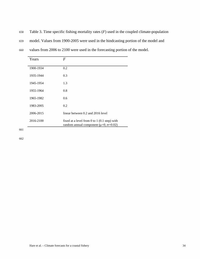
Table 3. Time specific fishing mortality rates (F) used in the coupled climate-population 658

model. Values from 1900-2005 were used in the hindcasting portion of the model and 659

values from 2006 to 2100 were used in the forecasting portion of the model. 660

Years F

1900-1934 0.2

1935-1944 0.3

1945-1954 1.3

1955-1964 0.8

1965-1982 0.6

1983-2005 0.2

2006-2015 linear between 0.2 and 2016 level

2016-2100 fixed at a level from 0 to 1 (0.1 step) with random annual component (μ=0, σ=0.02)

661

662


Table 4. Ensemble average maximum sustainable yield (MSY) and fishing rate at 663

maximum sustainable yield (FMSY) based on three CO2 emission scenarios simulated with 664

14 General Circulation Models (GCMs). Also provided are the values based on the most 665

recent stock assessment of Atlantic croaker (ASMFC 2005); the values presented here are 666

slightly different than those presented in the assessment because the model form used 667

here (an environmentally-explicit Ricker stock-recruitment function) is different than that 668

used in the stock assessment (a standard Beverton-Holt function). Multimodel ensemble 669

mean and 95% confidence intervals are provided. 670

671

Scenario FMSY Yield (MSY) (kg) Confidence Intervals (kg)

A1B 0.89 3.67 x 107 3.30-4.07 x 107

B1 0.78 3.23 x 107 2.90-3.58 x 107

Commit 0.62 2.52 x 107 2.24-2.82 x 107

Observed 0.48 1.87 x 107

672


Figure legends 673

Fig. 1. Relationship between Atlantic croaker recruitment and minimum winter air 674

temperature and comparison of observed recruitment and spawning stock biomass with 675

hindcasts developed from a coupled climate-population model. A) Relationship between 676

minimum winter air temperature in Virginia and recruitment of Atlantic croaker (r=0.68, 677

p<0.001). B) Environmental stock-recruitment relationship for Atlantic croaker (r2= 678

0.61, p<0.001). Estimates of recruitment are shown for three fixed temperatures. C and 679

D) Comparison of observed and modeled recruitment and spawning stock biomass from 680

1973 to 2003 based on the coupled climate-population model. Observed values (black 681

lines) are from the stock assessment (ASMFC 2005). Modeled values are shown as the 682

mean ± standard deviation of 100 runs of the coupled climate-population model. 683

684

Fig. 2. Observations and General Circulation Model (GCM) projections of minimum 685

winter air temperature in Chesapeake Bay region from 1900 to 2100. Results from three 686

CO2 emission scenarios averaged for 14 GCMs are shown. Long-term trends in 687

temperature are represented by a 30 point lowess smoother fit to the annual series; these 688

smoothed trends included a combination of observed and modeled temperatures so the 689

divergence between observations and models occurs prior to the end of the observations. 690

Lines represent the multimodel mean of the GCMs and shading represents 95% 691

confidence intervals. 692

693


Fig. 3. Forecasts of the effects of climate change on Atlantic croaker spawning stock 694

biomass for each of 14 General Circulation Models (GCMs) and three CO2 emission 695

scenarios at three fishing mortalities (F=0, F=-0.1, and F-=0.4). Historical levels (HM) of 696

spawning stock biomass are shown (1972-2004). 697

698

Fig. 4. A) Ensemble multimodel mean spawning stock biomass (2010 to 2100) for three 699

climate scenarios (commit, B1, and A1B) and a range of fishing mortality rates. B) 700

Contours of FS

CS

∂∂

∂∂ , which is a measure of the relative effect of climate compared to 701

fishing. Arrows along the x-axis indicate the current fishing mortality rate. 702

703

Fig. 5. Forecasts of the effect of climate change on Atlantic croaker distribution in the 704

mid-Atlantic region of the northeast U.S. continental shelf. Mean location, northern 705

extant, and frequency north of Hudson Canyon are shown based on three CO2 emission 706

scenarios from 14 General Circulation Models (GCMs) at three fishing mortalities (F=0, 707

F=-0.1, and F-=0.4). Historical levels (HM) of distribution measures are shown (1972-708

2004).. 709

710

Fig. 6. A) Ensemble multimodel mean population location, B) northern extent of the 711

range (mean + 2 standard deviations), and C) percent of years when northern extent of the 712

population is north of the Hudson Canyon (distance 600 km). D) Maps of various 713

distance marks along the continental shelf. The historical values (1972-2004) of mean 714

location (~240 km), northern extent (~420 km), and proportion of years with the measure 715


of northern extent exceeding 600 km (0.09) are shown as dark grey contours. Arrows 716

along the x-axis indicate the level of current fishing mortality rate. 717

718

Fig. 7. Fishery yield as a function of fishing mortality rate based on the temperature-719

dependent stock recruitment model (see Fig 1B) and ensemble multimodel mean of three 720

climate scenarios (commit, B1, and A1B). Yield curves are presented as lines; maximum 721

sustainable yields (MSY) and fishing rates at maximum sustainable yields (FMSY) are 722

indicated by triangles. 723

724


Figure 1


Figure 2


Figure 3


Figure 4


Figure 5


Figure 6


Figure 7

Hare et al. - Climate forecasts for Atlantic croaker 1

Online Appendix Forecasting the Dynamics of a Coastal Fishery Species Using a Coupled Climate-Population Model Jonathan Hare 1, Michael Alexander 2, Michael Fogarty 3, Erik Williams 4, James Scott 2 1. Background on general circulation models 2. Choice of a stock recruitment function 3. Distribution model based on logistic regression 4. References 1. Background on general circulation models

Annual minimum monthly winter air temperature was derived from 14 General Circulation Models (GCMs, Table A1). Also known as global climate models, GCMs depict the climate using a three dimensional grid over the globe, typically with horizontal resolutions between 250 and 600 km, 10 to 20 vertical layers in the atmosphere, and as many as 30 layers in the oceans. The resolution of these models is coarse and subgrid scale processes (e.g., turbulence in the boundary layer, thunderstorms and ocean eddies) are parameterized based on large-scale conditions, i.e., variables that are simulated on the model’s coarse grid. Even at coarse resolution, the models are run on super computers as the temperature, moisture, salinity, winds, ocean currents, etc., are predicted at hundreds of thousands of grid boxes.

GCMs can be verified by comparing their output to the recent past, e.g., how simulated and observed temperatures changed over the 20th century. An exact match between observations and model simulations in a given period is not expected because of random fluctuations in the climate system. To overcome the influence of random fluctuations in climate, the output of an ensemble of model runs (as opposed to a single model run) is generally compared to observations.

All the GCMs used here have simulations for the 20th century. Annual minimum monthly winter temperatures (minimum[Dec, Jan, Feb, and Mar]) for the grid cell over southern Chesapeake Bay was extracted from the 20th century runs and compared with observed minimum winter temperatures for Virginia (http://www.sercc.com/climateinfo_files/monthly/Virginia_temp.html). As an example the GFDL CM2.1 mean was about 0.5oC lower and the standard deviation was slightly greater than observed (Table A2). The mean differences of other models ranged from +10oC to -4oC. These mean differences between the climate models and observations were used to bias correct the minimum winter air temperatures estimated by each GCM. The smoothed observations indicate a long-term cycle in minimum winter air-temperature with high temperatures in the 1940’s and low temperatures in the 1970’s; these warm and cool periods have been linked to the Atlantic Multidecadal Oscillation (Kerr 2000, 2005). Some of the modeled temperatures do not match this long-term trend in observed temperature, but the modeled temperatures seem to exhibit a cycle of similar duration and magnitude as observed.

Prior studies have shown that GCMs generally reproduce the continental-scale trends (Randall et al. 2007) and some regional trends (Knutson et al. 2006, Seager et al. 2007). For example, the GFDL CM2.1 reproduces the observed warming over the 20th century in the subtropical North Atlantic and continental U.S. when anthropogenic forcing is included, but


Table A1. List of General Circulation Models (GCMs) used in this study. The institution and model name are provided, as are the links to the model metadata. For each GCM, three scenarios were used: commit, B1, and A1B. In addition, a 20th century simulation was compared to 20th century observations to develop a mean bias correction for each model. All model outputs were downloaded from the World Data Center for Climate, IPCC Data Distribution Centre (http://www.mad.zmaw.de/IPCC_DDC/html/SRES_AR4/index.html)

Bjerknes Centre for Climate Research BCM2.0 http://cera-www.dkrz.de/WDCC/ui/Compact.jsp?acronym=BCCR_BCM2.0_COMMIT_1 http://cera-www.dkrz.de/WDCC/ui/Compact.jsp?acronym=CGCM3.1_T47_SRESB1_1 http://cera-www.dkrz.de/WDCC/ui/Compact.jsp?acronym=BCCR_BCM2.0_SRESA1B_1 http://cera-www.dkrz.de/WDCC/ui/Compact.jsp?acronym=BCCR_BCM2.0_20C3M_1

Canadian Centre for Climate Modeling and Analysis CGCM3 http://cera-www.dkrz.de/WDCC/ui/Compact.jsp?acronym=CGCM3.1_T47_COMMIT_2 http://cera-www.dkrz.de/WDCC/ui/Compact.jsp?acronym=CGCM3.1_T47_SRESB1_1 http://cera-www.dkrz.de/WDCC/ui/Compact.jsp?acronym=CGCM3.1_T47_SRESA1B_1 http://cera-www.dkrz.de/WDCC/ui/Compact.jsp?acronym=CGCM3.1_T47_20C3M_1

Centre National de Recherches Meteorologiques CM3 http://cera-www.dkrz.de/WDCC/ui/Compact.jsp?acronym=CNRM_CM3_COMMIT_1 http://cera-www.dkrz.de/WDCC/ui/Compact.jsp?acronym=CNRM_CM3_SRESB1_1 http://cera-www.dkrz.de/WDCC/ui/Compact.jsp?acronym=CNRM_CM3_SRESA1B_1 http://cera-www.dkrz.de/WDCC/ui/Compact.jsp?acronym=CNRM_CM3_20C3M_1

Australia's Commonwealth Scientific and Industrial Research Mk3.0 http://cera-www.dkrz.de/WDCC/ui/Compact.jsp?acronym=CSIRO_Mk3.0_COMMIT_1 http://cera-www.dkrz.de/WDCC/ui/Compact.jsp?acronym=CSIRO_Mk3.0_SRESB1_1 http://cera-www.dkrz.de/WDCC/ui/Compact.jsp?acronym=CSIRO_Mk3.0_SRESA1B_1 http://cera-www.dkrz.de/WDCC/ui/Compact.jsp?acronym=CSIRO_Mk3.0_20C3M_1

Meteorological Institute, University of Bonn ECHO-G http://cera-www.dkrz.de/WDCC/ui/Compact.jsp?acronym=ECHO_G_COMMIT_1 http://cera-www.dkrz.de/WDCC/ui/Compact.jsp?acronym=ECHO_G_SRESB1_1 http://cera-www.dkrz.de/WDCC/ui/Compact.jsp?acronym=ECHO_G_SRESA1B_1 http://cera-www.dkrz.de/WDCC/ui/Compact.jsp?acronym=ECHO_G_20C3M_1

Institude of Atmospheric Physics FGOALS-g1.0 http://cera-www.dkrz.de/WDCC/ui/Compact.jsp?acronym=FGOALS_g1.0_COMMIT_1 http://cera-www.dkrz.de/WDCC/ui/Compact.jsp?acronym=FGOALS_g1.0_SRESB1_1 http://cera-www.dkrz.de/WDCC/ui/Compact.jsp?acronym=FGOALS_g1.0_SRESA1B_1 http://cera-www.dkrz.de/WDCC/ui/Compact.jsp?acronym=FGOALS_g1.0_20C3M_1

Geophysical Fluid Dynamics Laboratory CM2.1 http://cera-www.dkrz.de/WDCC/ui/Compact.jsp?acronym=GFDL_CM2.1_COMMIT_1 http://cera-www.dkrz.de/WDCC/ui/Compact.jsp?acronym=GFDL_CM2.1_SRESB1_1 http://cera-www.dkrz.de/WDCC/ui/Compact.jsp?acronym=GFDL_CM2.1_SRESA1B_1 http://cera-www.dkrz.de/WDCC/ui/Compact.jsp?acronym=GFDL_CM2.1_20C3M_1


Goddard Institute for Space Studies E-R http://cera-www.dkrz.de/WDCC/ui/Compact.jsp?acronym=GISS_ER_COMMIT_1 http://cera-www.dkrz.de/WDCC/ui/Compact.jsp?acronym=GISS_ER_SRESB1_1 http://cera-www.dkrz.de/WDCC/ui/Compact.jsp?acronym=GISS_ER_SRESA1B_1 http://cera-www.dkrz.de/WDCC/ui/Compact.jsp?acronym=GISS_ER_20C3M_1

Institute for Numerical Mathematics CM3.0 http://cera-www.dkrz.de/WDCC/ui/Compact.jsp?acronym=INM_CM3.0_COMMIT_1 http://cera-www.dkrz.de/WDCC/ui/Compact.jsp?acronym=INM_CM3.0_SRESB1_1 http://cera-www.dkrz.de/WDCC/ui/Compact.jsp?acronym=INM_CM3.0_SRESA1B_1 http://cera-www.dkrz.de/WDCC/ui/Compact.jsp?acronym=INM_CM3.0_20C3M_1

Institut Pierre Simon Laplace CM4 http://cera-www.dkrz.de/WDCC/ui/Compact.jsp?acronym=IPSL_CM4_COMMIT_1 http://cera-www.dkrz.de/WDCC/ui/Compact.jsp?acronym=IPSL_CM4_SRESB1_1 http://cera-www.dkrz.de/WDCC/ui/Compact.jsp?acronym=IPSL_CM4_SRESA1B_1 http://cera-www.dkrz.de/WDCC/ui/Compact.jsp?acronym=IPSL_CM4_20C3M_1

National Institute for Environmental Studies MIROC3.2 http://cera-www.dkrz.de/WDCC/ui/Compact.jsp?acronym=MIROC3.2_mr_COMMIT_1 http://cera-www.dkrz.de/WDCC/ui/Compact.jsp?acronym=MIROC3.2_mr_SRESB1_1 http://cera-www.dkrz.de/WDCC/ui/Compact.jsp?acronym=MIROC3.2_mr_SRESA1B_1 http://cera-www.dkrz.de/WDCC/ui/Compact.jsp?acronym=MIROC3.2_mr_20C3M_1

Meteorological Research Institute CGCM2.3.2 http://cera-www.dkrz.de/WDCC/ui/Compact.jsp?acronym=MRI_CGCM2.3.2_COMMIT_1 http://cera-www.dkrz.de/WDCC/ui/Compact.jsp?acronym=MRI_CGCM2.3.2_SRESB1_1 http://cera-www.dkrz.de/WDCC/ui/Compact.jsp?acronym=MRI_CGCM2.3.2_SRESA1B_1 http://cera-www.dkrz.de/WDCC/ui/Compact.jsp?acronym=MRI_CGCM2.3.2_20C3M_1

National Centre for Atmospheric Research CCSM3 http://cera-www.dkrz.de/WDCC/ui/Compact.jsp?acronym=NCAR_CCSM3_COMMIT_1 http://cera-www.dkrz.de/WDCC/ui/Compact.jsp?acronym=NCAR_CCSM3_SRESB1_1 http://cera-www.dkrz.de/WDCC/ui/Compact.jsp?acronym=NCAR_CCSM3_SRESA1B_1 http://cera-www.dkrz.de/WDCC/ui/Compact.jsp?acronym=NCAR_CCSM3_20C3M_1

UK Met. Office HadCM3 http://cera-www.dkrz.de/WDCC/ui/Compact.jsp?acronym=UKMO_HadCM3_COMMIT_1 http://cera-www.dkrz.de/WDCC/ui/Compact.jsp?acronym=UKMO_HadCM3_SRESB1_1 http://cera-www.dkrz.de/WDCC/ui/Compact.jsp?acronym=UKMO_HadCM3_SRESA1B_1 http://cera-www.dkrz.de/WDCC/ui/Compact.jsp?acronym=UKMO_HadGEM_20C3M_1

over-estimates warming for the southeast US (Knutson et al. 2007). All climate models have biases and several factors may lead to model-data differences including model error, inadequate representation of regional processes (e.g., aerosol loading, deforestation/reforestation, irrigation), and natural variability (i.e,. the atmospheric circulation over the southeast United States is influenced by El Nino and the Atlantic Multidecadal Oscillation). While there are differences between the GFDL CM2.1 and the observed annual temperature trends in the southeast U.S., there is general agreement between the simulated and observed minimum winter temperature in the GCMs considered here (Figure A1 and Table A2).


Fig. A1. Distributions of observed and modeled reanalysis minimum winter air temperatures and comparison of observed and predicted means and standard deviations of temperature (top row). Time series of observations and GCM predicted minimum winter temperatures. Also shown is the corrected model estimate based on adding the mean model-vs-observation difference to the model. Smoothed observations and predictions, with the predictions corrected by the mean difference between model and observations (bottom row). Results are shown for the ECHOG GCM; similar analyses were done for all GCMs. Observations are minimum monthly winter temperature in Virginia and model results are from the grid cell encompassing Chesapeake Bay.

Although, the analyses above suggest that the climate models reasonably capture the minimum monthly winter air temperatures in coastal Virginia, a potential concern is that the coupled climate-population model results are specific for this model grid cell. However, there is strong concordance in the time series of minimum winter air temperature over the eastern seaboard of the United States (Fig. A3) in historical observations and climate model hindcasts

Table A2. Mean correction bias for each GCM. The average simulated minimum winter air temperature was compared to the average observed minimum winter air temperature over the 20th century. The difference in averages was added to the GCM simulated minimum winter air temperatures. A comparison of standard deviations is also provided.

Observed Minimum Winter Temperature

Mean Standard Deviation

0.65 2.00

Difference between observed and modeled temperatures

GCM Mean Standard Deviation

BCM2.0 6.48 -0.59

CGCM3 -2.55 0.28

CM3 3.27 -0.37

MK3.0 -1.84 0.02

ECHO-G 2.75 -0.51

FGOALS g1.0 9.94 -0.44

CM2.1 -0.54 0.21

E-R -3.71 0.28

CM3.0 2.78 -0.05

CM4 4.20 -0.08

MIROC3.2 8.79 -0.81

CGCM2.3.2 1.11 -0.42

CCSM3 3.06 -0.10

HadCM3 7.80 -0.10


Fig. A2. Time series of minimum winter air temperatures from the NCEP Reanalysis for grid cells nearest the locations indicated on the map. These data were significantly concordant: the pattern of interannual variability was coherent across the time series.

(Table A3). This concordance is expected since prior studies have documented strong concordance in interannual winter air temperature over the eastern U.S. (Joyce 2002), estuarine water temperatures in the mid-Atlantic (Hare and Able 2007), coastal water temperatures (Nixon et al. 2004), and sea surface temperature in the western North Atlantic (Friedland and Hare 2007). Additionally, minimum winter air temperature is closely related to minimum winter water temperature in estuaries along the mid-Atlantic coast (Hettler and Chester 1982, Hare and Able 2007) owing to the efficient heat exchange between atmosphere and water in these shallow systems (Roelofs and Bumpus 1953). Thus, minimum winter air temperatures from Virginia can serve as a proxy for coast-wide variability in minimum winter water temperatures. 2. Choice of a stock-recruitment function

A number of functions have been used historically to model the relationship between fish population size and subsequent recruitment (Hilborn and Walters 2004). There also are a number of extensions of these functions that include the effect of the environment on recruitment (Hilborn and Walters 2004). We evaluated two common stock recruitment functions (Beverton-


Holt and Ricker) and several extensions of these functions that include environmental effects (Table A4). The Akaike Information Criterion (AIC) was used to choose the best formulation to use in the coupled climate-population model. Spawning stock biomass and recruitment data were obtained from a recent stock assessment of Atlantic croaker (ASMFC 2005) and minimum winter air temperature in Virginia (http://www.sercc.com/climateinfo_files/monthly/Virginia_temp.html) was used as a proxy for water temperature during the estuarine juvenile stage (Hare and Able 2007).

The stock-recruitment functions were initially fit with non-linear algorithms, but these algorithms rarely converged. As a result, linear forms of the stock recruitment functions (model 1 and 4, see Table A4) were fit using least-squares regression. The environmental extensions of the Ricker stock-recruitment model are easily linearized (models 5-11, see Table A4) and these models were also fit using least-squares. The environmental forms for the Beverton-Holt model (models 2 and 3) are not easily linearized. To fit these models, the standard Beverton-Holt terms (a and b) were estimated using the linearized version of the model (model 1), and then a non-linear fitting algorithm was used to estimate the environmental parameter (c) with the standard parameters (a and b) fixed at the appropriate values. Because the linearized forms of the models used different dependent variables (1/R for Beverton and Holt and ln[R/S] for Ricker), AIC was estimated based on the models predictions of R using the non-linearized forms of the equations, with the terms derived from the linearized models. In this way, AIC was calculated based on the residual sums of squares of estimated R and observed R. The strength of evidence of the alternative models was calculated following (Burnham and Anderson 1998).

The Ricker stock-recruitment model with a temperature term was the best-supported model evaluated (Table A4), with the highest strength of evidence (w=0.619). The models with environmental terms were far superior to the standard stock-recruitment models. The relative likelihood of the environmental Beverton and Holt model (model 2) compared to the standard

Table A3. Kendall’s concordance (W) for time series of minimum winter air temperatures from locations indicated in Fig. A3. Calculations were made for each of the models considered based on the 20th century runs. Kendall’s concordance is a non-parametric test that measures the degree of agreement between multiple series of data: 0 indicates no agreement; 1 indicates perfect agreement. The NCEP/NCAR Reanalysis Product was also included in these analyses. This product is a gridded dataset based on retrospective observations (1948-2006) of a variety of atmospheric variables including surface temperature (Kalnay et al. 1996).

General Circulation Model W p Years NCEP Analysis 0.73 <0.001 1948-2006 BCM2.0 0.60 <0.001 1850-2000 CGCM3 0.62 <0.001 1850-2001 CM3 0.63 <0.001 1860-2000 MK3.0 0.61 <0.001 1871-2001 ECHO-G 0.59 <0.001 1860-2001 FGOALS g1.0 0.64 <0.001 1850-2000 CM21 0.61 <0.001 1861-2001 E-R 0.52 <0.001 1880-2004 HadCM3 0.58 <0.001 1860-2000 CM3.0 0.40 <0.001 1871-2001 CM4 0.67 <0.001 1860-2001 MIROC3.2 0.60 <0.001 1850-2001 CGCM2.3.2 0.67 <0.001 1851-2001 CCSM3 0.60 <0.001 1870-2000


Beverton and Holt model was ~6000 to 1 (wmodel 2 / wmodel 1). For the environmental Ricker (model 5) compared to the standard Ricker (model 4), the relative likelihood was ~10000 to 1. Based on these results, model 5 was chosen for use in the population model. Temperature-dependent Ricker models with higher order terms (model 8 and 9) had moderate strengths of evidence (w=0.137 and w=0.181). Model 8 includes a T2 term, which could amplify the effect of warming on recruitment at higher minimum winter temperatures. However, over the range of temperatures forecasted in the climate models, the higher order models (model 8 and 9) predict very similar recruitment compared to the linear model (model 5), so non-linear effects are minimal, and thus these were not included in the final model.

Table A4. Akaike Information Criteria values for various models fit to stock (S) and recruitment (R) data for the mid-Atlantic stock of Atlantic croaker. Values provided for corrected Akaike Information Criteria (AICc), number of parameters in the model including the error term (k), the delta-AICc, which is scaled to the minimum observed AICc, and the model weights (w), which range from 0 to 1. No. Model Linearized Model AICc k ΔAICc W

1 aSb

SR+

= Sba

R+=

1 309.1 3 24.6 0.000

2 aSbSeR

cT

+= Not linearized 291.5 4 7.0 0.019

3 aSeb

SR cT+= Not linearized 294.6 4 10.1 0.004

4 bSaSeR += bSaSR

+=)ln( 303.4 3 18.9 0.000

5 cTbSaSeR ++= cTbSaSR

++=)ln( 284.5 4 0.0 0.619

6 2dTbSaSeR ++= 2)ln( dTbSa

SR

++= 306.2 4 21.7 0.000

7 eSTbSaSeR ++= eSTbSaSR

++=)ln( 293.4 4 8.9 0.007

8 2dTcTbSaSeR +++= 2)ln( dTcTbSa

SR

+++= 287.5 5 3.0 0.137

9 eSTcTbSaSeR +++= eSTcTbSaSR

+++=)ln( 287.0 5 2.5 0.181

10 eSTdTbSaSeR +++=2

eSTdTbSaSR

+++= 2)ln( 295.8 5 11.3 0.002

11 eSTdTcTbSaSeR ++++=

2

eSTdTcTbSa

SR

++++= 2)ln( 290.5 6 6.0 0.031


3. Distribution model based on logistic regression

A multivariate regression approach was used to model distribution as a function of population size and winter temperature. The hypothesis was that as population size increased and winter temperatures increased the mean and northern extent of the population (mean + 2 standard deviations) would shift northward. A shift in mean location is not necessarily predicted with increasing population size; the mean could remain stationary and the northern and southern extents of the population could expand. However, in the case of Atlantic croaker, sampling did not occur throughout the range of the population; sampling stopped at a fixed geographic location, so an expansion in the southern range would not be observed. Thus as the northern range extends and the southern boundary of sampling remains stationary a northward shift in the mean location is predicted.

As an alternative approach to multiple regression for modeling distribution, a logistic regression was developed that used the presence / absence at individual trawl stations. First, trawl stations were screened to remove stations that sampled deeper than 45 m; this value was based on the 5% level of a logistic regression of catch on depth. The logistic regression model was used in a form similar to the average distance model. Catch at station s in year Y was modeled as the distance of station s in year Y, spawning stock biomass (S) in year Y, and minimum winter temperature in year Y:

22

YYYYsYsY TfSSBeTdSSBcdistbacatch ⋅+⋅+⋅+⋅+⋅+= (6) The model was fit using the glm [family=binomial(link="logit")] function in R (http://www.r-project.org/) and an Akaike multi-model inference was used to determine the model parameters. The model was then used to forecast Atlantic croaker distribution estimating the distance to the 50% and 10% catch probability. The results were qualitatively similar to those from the average distance approach, with distances decreasing with increasing F and increasing with increasing CO2 emissions; we choose to present the results of the multiple regression model.

4. References ASMFC, A. S. M. F. C. 2005. Atlantic croaker stock assessment and peer-review reports.

Atlantic States Marine Fisheries Commission, Washington, D.C.

Burnham, K. P., and D. R. Anderson. 1998. Model selection and multimodel inference: a

practical information-theoretic approach. Springer, New York.

Friedland, K. F., and J. A. Hare. 2007. Long-term trends and regime shifts in sea surface

temperature on the continental shelf of the northeast United States. Continental Shelf

Research 27:2313-2328.


Hare, J. A., and K. W. Able. 2007. Mechanistic links between climate and fisheries along the

east coast of the United States: explaining population outbursts of Atlantic croaker

(Micropogonias undulatus). Fisheries Oceanography 16:31-45.

Hettler, W. F., and A. J. Chester. 1982. The relationship of winter temperature and spring

landings of pink shrimp, Penaeus duorarum, in North Carolina. Fishery Bulletin 80:761-

768.

Hilborn, R., and C. Walters. 2004. Quantitative fisheries stock assessment - choice, dynamics

and uncertainty Kluwer Academic Publishers, Norwell, Massachusetts.

Joyce, T. M. 2002. One hundred plus years of wintertime climate variability in the eastern

United States. Journal of Climate 15:1076-1086.

Kalnay, E., M. Kanamitsu, R. Kistler, W. Collins, D. Deaven, L. Gandin, M. Iredell, S. Saha, G.

White, J. Woollen, Y. Zhu, A. Leetmaa, R. Reynolds, M. Chelliah, W. Ebisuzaki, W.

Higgins, J. Janowiak, K. C. Mo, C. Ropelewski, J. Wang, R. Jenne, and D. Joseph. 1996.

The NCEP/NCAR 40-Year Reanalysis Project. Bulletin of the American Meteorological

Society 77:437-471.

Kerr, R. A. 2000. A North Atlantic climate pacemaker for the centuries. Science 288:1984-1986.

Kerr, R. A. 2005. Atlantic climate pacemaker for millennia past, decades hence? Science 309:43-

44.

Knutson, T. R., T. L. Delworth, K. W. Dixon, I. M. Held, J. Lu, V. Ramaswamy, M. D.

Schwarzkopf, G. Stenchikov, and R. J. Stouffer. 2006. Assessment of Twentieth-Century

regional surface temperature trends using the GFDL CM2 coupled models. Journal of

Climate 10:1624-1651.

Nixon, S. W., S. Granger, B. A. Buckley, M. Lamont, and B. Rowell. 2004. A one hundred and

seventeen year coastal water temperature record from Woods Hole, Massachusetts.

Estuaries 27:397-404.

Randall, D. A., R. A. Wood, S. Bony, R. Colman, T. Fichefet, J. Fyfe, V. Kattsov, A. Pitman, J.

Shukla, J. Srinivasan, R. J. Stouffer, A. Sumi, and K. E. Taylor. 2007. Cilmate Models

and Their Evaluation.in S. Solomon, D. Qin, M. Manning, Z. Chen, M. Marquis, K. B.

Averyt, M. Tignor, and H. L. Miller, editors. Climate Change 2007: The Physical Science

Basis. Contribution of Working Group I to the Fourth Assessment Report of the


Intergovernmental Panel on Climate Change. Cambridge University Press, Cambridge,

United Kingdom and New York, NY, United States.

Roelofs, E. W., and D. F. Bumpus. 1953. The hydrography of Pamlico Sound. Bulletin of Marine

Science of the Gulf and Caribbean 3:181-205.

Seager, R., M. F. Ting, I. Held, Y. Kushnir, J. Lu, G. Vecchi, H. P. Huang, N. Harnik, A.

Leetmaa, N. C. Lau, C. H. Li, J. Velez(Miller), N. Naik, and -. Science. 2007. Model

projections of an imminent transition to a more arid climate in southwestern North

America. . Science 316:1181-1184.

forecasting the dynamics of a coastal fishery species ... · forecasting the dynamics of a coastal...

Documents