forecasting stock returns under economic constraints
TRANSCRIPT

Contents lists available at ScienceDirect
Journal of Financial Economics
Journal of Financial Economics ] (]]]]) ]]]–]]]
http://d0304-40
☆ WeWe alsPastor, SmetricBayesia2013 Wcommetance. Wtheir co
n CorrE-m
atimmervalkan
1 Te2 Te
PleasEcon
journal homepage: www.elsevier.com/locate/jfec
Forecasting stock returns under economic constraints$
Davide Pettenuzzo a,1, Allan Timmermann b,c,d,2, Rossen Valkanov b,n
a Brandeis University, Sachar International Center, 415 South St, Waltham, MA, United Statesb University of California, San Diego, 9500 Gilman Drive, MC 0553, La Jolla, CA 92093, United Statesc CEPR, United Kingdomd CREATES, Denmark
a r t i c l e i n f o
Article history:Received 9 May 2013Received in revised form24 October 2013Accepted 21 November 2013
JEL classification:C11C22G11G12
Keywords:Economic constraintsSharpe ratioEquity premium predictions
x.doi.org/10.1016/j.jfineco.2014.07.0155X/& 2014 Elsevier B.V. All rights reserved.
thank an anonymous referee for many cono thank John Campbell, Wayne Ferson, Beth Pruitt, Guofu Zhou, seminar participantSociety Summer Institute and the 2013 Eun Econometrics, as well as Anthony Lynch, oestern Finance Association meetings in Laknts and suggestions. Xia Meng provided exce are grateful to John Campbell and David
des available.esponding author. Tel.: +1 858 534 0898.ail addresses: [email protected] (D. [email protected] (A. Timmermann),[email protected] (R. Valkanov).l.: +1 781 736 2834.l.: +1 858 534 0894.
e cite this article as: Pettenuzzo, D.,omics (2014), http://dx.doi.org/10.1
a b s t r a c t
We propose a new approach to imposing economic constraints on time series forecasts ofthe equity premium. Economic constraints are used to modify the posterior distribution ofthe parameters of the predictive return regression in a way that better allows the model tolearn from the data. We consider two types of constraints: non-negative equity premiaand bounds on the conditional Sharpe ratio, the latter of which incorporates time-varyingvolatility in the predictive regression framework. Empirically, we find that economicconstraints systematically reduce uncertainty about model parameters, reduce the risk ofselecting a poor forecasting model, and improve both statistical and economic measuresof out-of-sample forecast performance.
& 2014 Elsevier B.V. All rights reserved.
structive comments.lake LeBaron, Luboss at the 2013 Econo-ropean Seminar onur discussant at thee Tahoe, for helpfulellent research assis-Rapach for making
ttenuzzo),
et al., Forecasting stoc016/j.jfineco.2014.07.01
1. Introduction
Equity premium (EP) forecasts play a central role inareas as diverse as asset pricing, portfolio allocation, andperformance evaluation of investment managers.3 How-ever, more than 25 years of research shows that modelsallowing for time-varying return predictability often pro-duce worse out-of-sample forecasts than a simple bench-mark that assumes a constant risk premium. This findinghas led authors such as Bossaerts and Hillion (1999) andWelch and Goyal (2008) to question the economic value of
3 Papers on time series predictability of stock returns include Campbell(1987), Campbell and Shiller (1988), Fama and French (1988, 1989), Ferson andHarvey (1991), Keim and Stambaugh (1986) and Pesaran and Timmermann(1995). Examples of asset allocation studies under return predictability includeAït-Sahalia and Brandt (2001), Barberis (2000), Brennan, Schwartz, and Lagnado(1997), Campbell and Viceira (1999), Kandel and Stambaugh (1996), and Xia(2001). Avramov and Wermers (2006) and Ferson and Schadt (1996) considermutual fund performance under time-varying investment opportunities.
k returns under economic constraints. Journal of Financial5i
D. Pettenuzzo et al. / Journal of Financial Economics ] (]]]]) ]]]–]]]2
ex ante return forecasts that allow for time-varyingexpected returns.
Economically motivated constraints offer the potentialto sharpen forecasts, particularly when the data are noisyand parameter uncertainty is a concern as in returnprediction models. While economic constraints have pre-viously been found to improve forecasts of asset returns,no broad consensus exists on how to impose such con-straints. For example, Ang and Piazzesi (2003) impose no-arbitrage restrictions to identify the parameters in a termstructure model, Campbell and Thompson (2008) truncatetheir equity premium forecasts at zero and also constrainthe sign of the slope coefficients in return predictionmodels, and Pastor and Stambaugh (2009, 2012) useinformative priors to ensure that the sign of the correla-tion between shocks to unexpected and expected returnsis negative.
This paper proposes a new approach for incorporatingeconomic information via inequality constraints onmoments of the predictive distribution of the equitypremium. We focus on two types of economic constraints.The first, the equity premium constraint, follows the ideaof Campbell and Thompson (2008) and requires theconditional mean of the equity premium to be non-negative.4 It is difficult to imagine an equilibrium settingin which risk averse investors would hold stocks if theirexpected compensations were negative, and so this seemslike a mild restriction. The second stipulates that theconditional Sharpe ratio (SR) has to lie between zero anda predetermined upper bound. The zero lower bound isidentical to the equity premium constraint, and the upperbound rules out that the price of risk becomes too high.The Sharpe ratio of the market portfolio is extensivelyused in finance and, much like the equity premium,academics and investors can be expected to have strongpriors about its magnitude.5 Yet, SR constraints cast asinequality constraints on the predictive moments of thereturn distribution have not, to our knowledge, previouslybeen explicitly explored in the return predictabilityliterature.6
Other studies consider bounds on the maximum Sharperatio in the context of cross-sectional pricing models, whichis different from our focus here. MacKinlay (1995) intro-duces a bound on the maximum squared Sharpe ratio as a
4 Boudoukh, Richardson, and Smith (1993) develop tests for therestriction that the conditional equity risk premium is non-negative.They find that this restriction is violated empirically for the US stockmarket.
5 See Lettau and Wachter (2007, 2011) for recent examples oftheoretical asset pricing models that rely on calibrations using the Sharperatio. For good treatments of the Sharpe ratio and its theoretical andempirical links to asset pricing models, see Cochrane (2001) and Lettauand Ludvigson (2010).
6 Ross (2005) and Zhou (2010) consider constraints on the R2 of thepredictive return distribution. In practice, a close relation exists betweenconstraints on the Sharpe ratio and constraints on the R2. See, e.g.,Campbell and Thompson (2008) for investors with mean variance utility.Wachter and Warusawitharana (2009) also consider priors on the slopecoefficient in the return equation, which translate into priors about thepredictive R2 of the return equation. Shanken and Tamayo (2012) studyreturn predictability by allowing for time-varying risk and specify a prioron the Sharpe ratio.
Please cite this article as: Pettenuzzo, D., et al., Forecasting stocEconomics (2014), http://dx.doi.org/10.1016/j.jfineco.2014.07.01
way to distinguish between risk and nonrisk explanationsof deviations from the Capital Asset Pricing Model (CAPM).MacKinlay and Pastor (2000) provide estimates of factorpricing models that condition on a given value of theSharpe ratio. In a Bayesian setting, this corresponds toinvestors having different degrees of confidence in the assetpricing model, with a very large Sharpe ratio correspondingto completely skeptical beliefs about the model.
To incorporate economic information, we develop aBayesian approach that lets us compute the predictivedensity of the equity premium subject to economic con-straints. Importantly, the approach makes efficient use of theentire sequence of observations in computing the predictivedensity and also accounts for parameter uncertainty. Ourapproach builds on the conventional linear prediction modeland simplifies to this model if the economic constraints arenot binding in a particular sample.
The predictive moments of the return distribution getupdated as new data arrive and so the inequality con-straints give rise to dynamic learning effects. To see howthis works, suppose a new observation arrives that, underthe previous parameter estimates, imply a negative con-ditional equity premium. Because this is ruled out, theeconomic constraints can force the posterior distributionof the parameter estimates to shift significantly, evenin situations in which the estimates of the standard linearmodel do not change at all. This effect turns out to beempirically important, particularly for large values of thepredictor variables. Our empirical analysis finds that theposterior variance of the equity premium distribution—one measure of parameter estimation uncertainty—can beseveral times bigger for the unconstrained model com-pared with the constrained models, when evaluated atlarge values of the predictor variables.
Our approach toward incorporating economic constraintsworks very differently from that taken by previous studiessuch as Campbell and Thompson (2008). To highlight thesedifferences, consider the constraint that the equity premiumis non-negative. Campbell and Thompson (2008) impose thisrestriction by truncating the predicted equity premium atzero if the predicted value is negative. While this truncationapproach can be viewed as a first approximation towardimposing moment or parameter constraints, it does notmake efficient use of the information in the theoreticalconstraints. In particular, this approach never learns fromthe information that comes from observing that the esti-mated model implies negative forecasts of the equity pre-mium and so the underlying model continues to repeat thesame mistakes when faced with new data similar to pre-viously observed data. In contrast, our approach constrainsthe equity premium forecast to be non-negative at eachgiven time. This implies that we have T constraints in asample of T observations, not just a single constraint. Everytime a new pair of observations on the predictor variable andreturns becomes available, the non-negativity constraint onthe conditional equity premium is used to rule out values ofthe parameters that are infeasible given the constraint and,hence, to inform the parameter estimates.
In addition to the conditional EP constraint, we explorewhether imposing a lower and an upper bound on theSharpe ratio of the market portfolio provides further
k returns under economic constraints. Journal of Financial5i

D. Pettenuzzo et al. / Journal of Financial Economics ] (]]]]) ]]]–]]] 3
improvements. An upper bound on the Sharpe ratio isequivalent to a time-varying upper bound on the equitypremium that is proportional to the market volatility.The implementation of such a constraint is nontrivial as itinvolves modeling the conditional volatility of the marketportfolio in a predictive regression framework. We use aparsimonious parameterization that allows us to explore timevariation in the conditional first and second moments ofreturns. We find that the SR constraint increases the statisticaland economic gains not only relative to the unconstrainedcase, but also relative to the EP constraint.
Attempts at producing improved forecasts of stockreturns have spawned a huge literature that originatedfrom studies by Campbell (1987), Campbell and Shiller(1988), Fama and French (1988, 1989), Ferson and Harvey(1991), and Keim and Stambaugh (1986), who provideconvincing economic arguments and in-sample empiricalresults that some of the fluctuations in returns are pre-dictable because of persistent time variation in expectedreturns. In-sample evidence for predictability is accumu-lating as various new variables have been suggested aspredictors of excess returns (Pontiff and Schall, 1998;Lamont, 1998; Lettau and Ludvigson, 2001; Polk,Thompson, and Vuolteenaho, 2006, among others). Out-of-sample predictability evidence, however, has beenmuch less conclusive. Paye and Timmermann (2006) andLettau and Van Nieuwerburgh (2008) argue that predict-ability weakened or disappeared during the 1990s.Bossaerts and Hillion (1999), Goyal and Welch (2003),and Welch and Goyal (2008) provide an even sharpercritique by arguing that predictability was largely an in-sample or ex post phenomenon that disappears once theforecasting models are used to guide forecasts on new,out-of-sample, data. Rapach and Zhou (2013) provide anextensive review of this literature.
To evaluate our approach empirically, we considerthe large set of predictor variables used by Welch andGoyal (2008). When implemented along the lines proposedin our paper, for nearly all of the predictors and at themonthly, quarterly and annual frequencies, both the EP andSR constraints lead to substantial improvements in thepredictive accuracy of the equity premium forecasts. Acrossall variables, we find that when comparing the uncon-strained with the EP-constrained forecasts, the average out-of-sample R2 improves from �0.53% to 0.19% at themonthly frequency, from �2.33% to 0.47% at the quarterlyfrequency, and from �5.27% to 3.10% at the annual fre-quency. Similarly, comparing the unconstrained with the SRconstrained forecasts, the out-of-sample R2 improves from�0.53% to 0.18% at the monthly frequency, from �2.33% to1.02% at the quarterly frequency, and from �5.27% to 4.11%at the annual frequency. Hence, the improvement in pre-dictive accuracy tends to get larger as the forecast horizon isextended and the effect of estimation error in a conven-tional unconstrained model gets stronger.
Our empirical results corroborate that the Campbelland Thompson (2008) truncation approach improves onthe unconstrained forecasts for a clear majority ofthe predictors. However, we also find that imposing theEP constraint leads to an even larger gain in predictiveaccuracy, relative to the truncation approach, than the
Please cite this article as: Pettenuzzo, D., et al., Forecasting stocEconomics (2014), http://dx.doi.org/10.1016/j.jfineco.2014.07.01
truncation approach produces relative to the uncon-strained case. Specifically, at the monthly horizon, thepredictive accuracy improves for 14 out of 16 predictorsand increases the average out-of-sample R2 value by 0.4%.Similar results are found at the quarterly and annualhorizons, for which the EP constraint improves the averageout-of-sample R2 value by 1.5% and 5.2%, respectively, overthe truncated models.
We also consider the economic value of using con-strained forecasts in the portfolio allocation of a represen-tative investor endowed with power utility. In thebenchmark case with a coefficient of relative risk aversionof five, we compare the certainty equivalent return (CER)obtained from using a given predictor relative to theprevailing mean model. The comparison is conducted forthe unconstrained as well as the EP-constrained and theSR-constrained cases at monthly, quarterly, and annualhorizons, for the entire sample and a few subsamples.Here, again, we find that the economic constraints lead tohigher CER values at all horizons and across practically allpredictors (the one exception being the stock variance).Specifically, the EP constraint results in a higher CER(relative to the unconstrained case) of 40–50 basis pointsper year. For the SR-constrained models, the increase isabout twice as high. Consistent with the predictive accu-racy results, we generally find that the SR constraintproduces higher CER improvements than the EP con-straint, which suggests that economically important inter-actions exist between the estimated mean and volatility.Robustness checks reveal that a higher (lower) risk aver-sion coefficient of 10 (2) reduces (increases) the spread inperformance across models, as the investor's willingnessto exploit any predictability is inversely proportional to therisk aversion.
The previous results refer to univariate regressionmodels with a single predictor variable. We also considertwo ways to incorporate multivariate information. First,we consider equal-weighted forecast combinations. Con-sistent with Rapach, Strauss, and Zhou (2010), we find thatsimple forecast combinations improve on the averageforecast performance, particularly for the unconstrainedforecasts that are most adversely affected by parameterestimation error. Second, we consider a diffusion indexapproach that extracts common components from thecross-section of predictor variables followed by uncon-strained or constrained equity premium predictions usingthese components. Empirically, the diffusion indexapproach produces better statistical and economic perfor-mance than the equal-weighted combination approachboth across subsamples and in the full sample. Moreover,this approach works best for the economically constrainedmodels. For example, at the quarterly horizon, the out-of-sample R2 of the diffusion index is 0.42%, 3.02%, and 2.95%for the unconstrained, EP-constrained, and SR-constrainedmodels, respectively, with associated CER values of �0.04%,0.53%, and 0.95% per annum.
The plan of the paper is as follows. Section 2 introducesour new methodology for efficiently incorporating theore-tical constraints on the predictive moments of the equitypremium distribution. Section 3 introduces the data andpresents empirical results for both unconstrained and
k returns under economic constraints. Journal of Financial5i

Fig. 1. Equity premium constraint. This figure shows the effect on the parameters μ (shown on the x-axis) and β (shown on the y-axis) from imposing theequity premium constraint μþβxtZ0, as indicated by the shaded area. The solid and dotted lines correspond to the cases in which the predictor value is setto the smallest and largest values attained in sample, and the dashed line depicts the case in which the predictor value is set to its sample average. (a) Logdividend–price ratio, �4:52rxtr�1:87, (b) T-bill rate, 0:0001rxtr0:163, (c) Log dividend–payout ratio, �1:22rxtr1:38.
D. Pettenuzzo et al. / Journal of Financial Economics ] (]]]]) ]]]–]]]4
constrained prediction models using a range of predictorvariables. Section 4 evaluates the economic value ofimposing economic constraints on the forecasts. Section 5presents an extension to incorporate multivariate informa-tion and conducts a range of robustness tests, and Section 6concludes.
2. Methodology
This section describes how we estimate and forecastthe equity premium subject to constraints motivated byeconomic theory. These constraints take the form of
Please cite this article as: Pettenuzzo, D., et al., Forecasting stocEconomics (2014), http://dx.doi.org/10.1016/j.jfineco.2014.07.01
inequalities on the conditional equity premium or boundson the conditional Sharpe ratio.
2.1. Economic constraints on the return prediction model
The literature on return predictability commonlyassumes that stock returns, measured in excess of a risk-free rate, rτþ1, is a linear function of lagged predictorvariables, xτ:
rτþ1 ¼ μþβxτþετþ1; τ¼ 1;…; t�1;
ετþ1 �Nð0;σ2εÞ: ð1Þ
k returns under economic constraints. Journal of Financial5i

Exc
ess
retu
rns
(per
cent
)
1920 1925 1930 1935 1940 1945 1950−0.4
−0.2
0
0.2
0.4
0.6
0.8
1
1.2
1.4
1.6
Fig. 2. Comparison of in-sample fitted values and out-of-sample forecast under the equity premium constraint and the truncation approach. This figurecompares the in-sample fitted values and out-of-sample predicted excess return for January 1947 under the equity premium constraint versus under thetruncation approach of Campbell and Thompson (2008; CT truncated). We regress excess returns ðrtþ1Þ on an intercept and the lagged log dividend–priceratio, xt over the period January 1927–December 1946: rtþ1 ¼ μþβxtþεtþ1. Estimates from this model are then used to generate in-sample fitted valuesas well as a one-step out-of-sample forecast of excess returns for January 1947. The equity premium constrained model imposes thatr̂ τþ1jt ¼
R ðμþβxτÞpðμ; βjDt Þ dμ dβ40; for τ¼ 1;…; t and information set Dt .
D. Pettenuzzo et al. / Journal of Financial Economics ] (]]]]) ]]]–]]] 5
The linear model is simple to interpret and requires estimat-ing only two mean parameters, μ and β, which can readily beaccomplished by ordinary least squares (OLS).
Economic theory generally does not restrict the functionalform of the mapping linking predictor variables, xτ , to theconditional mean of excess returns, rτþ1, so the use of thelinear specification in Eq. (1) should be viewed as anapproximation. However, we argue that economically moti-vated constraints can be used to improve on this model.
2.1.1. Equity premium constraintUnder broad conditions, the conditional equity risk
premium can be expected to be positive.7 This reasoningimplies a constraint on the predictive moments of thedistribution of excess returns. In turn, this has implicationsfor the estimated parameters of the return predictionmodel equation (1). Specifically, to efficiently exploit theinformation embedded in the constraint that the condi-tional equity premium is nonnegative, the parameters μand β should be estimated subject to the constraintμþβxτZ0 at all times8:
μþβxτZ0 for τ¼ 1;…; t: ð2Þ
7 For example, this rules out that stocks hedge against other riskfactors affecting the performance of a market portfolio composed of abroader set of asset classes.
8 Here t refers to the present time, τ¼ 1;…; t�1 indexes all historical(in-sample) observations up to the present point and the out-of-sampleforecast is obtained for τ¼ t.
Please cite this article as: Pettenuzzo, D., et al., Forecasting stocEconomics (2014), http://dx.doi.org/10.1016/j.jfineco.2014.07.01
Although this constraint on the predictive moments of theequity premium is not directly a constraint on the modelparameters, θ¼ ðμ;β;σ2
εÞ, it clearly affects these para-meters because they have to be consistent with Eq. (2).Moreover, because the conditional EP constraint has tohold at each time, the number of constraints grows inproportion to the length of the sample size. The seeminglysimple EP constraint in Eq. (2), therefore, potentially yieldsa powerful way to pin down the parameters of the returnforecasting model and obtain more precise estimates.
To see how the constraint in Eq. (2) works to restrictthe μ�β parameter space, consider Fig. 1. Panel a showshow different values of x constrain the admissible set of μand β values when x is always negative (e.g., log dividendyield case). Panel b repeats this exercise when x takes ononly positive values (T-bill case), and Panel c illustrates thecase with a predictor that can take on both negative andpositive values (log dividend payout ratio case). Thesegraphs illustrate that whenever a new observation of xarrives, both small and large values of this predictor canlead to new constraints on the set of feasible parametervalues. Moreover, there are T constraints on the para-meters in a sample with T observations.
Campbell and Thompson (2008, CT) were the first toargue in favor of imposing a non-negative EP constraint.9
They implement this idea by using a truncated forecast,
9 Prior to this, some papers tested non-negativity of the equitypremium. For example, Ostdiek (1998) studies sign restrictions on theex ante equity premium and develops tests for whether this premium isnon-negative using a conditional multiple inequality approach.
k returns under economic constraints. Journal of Financial5i

μ
Intercept
1935 1940 1945 1950 1955 1960 1965 1970 1975 1980 1985 1990 1995 2000 2005−2
0
2
4
6
8
10x 10−3
β
Slope coefficient
1935 1940 1945 1950 1955 1960 1965 1970 1975 1980 1985 1990 1995 2000 2005−0.1
−0.05
0
0.05
0.1
0.15
0.2
0.25
0.3
Fig. 3. Comparison of coefficient estimates under the equity premium constraint and the Campbell and Thompson (2008) truncation approach. This figureshows a comparison of the posterior means of the coefficient estimates in the excess return regression rtþ1 ¼ μþβxtþεtþ1. The truncation approach usesunconstrained ordinary least squares to estimate the coefficient estimates, whereas the equity premium constrained model imposes thatr̂ τþ1jt ¼
R ðμþβxτÞpðμ; βjDt Þ dμ dβ40; for τ¼ 1;…; t and information set Dt . Coefficient estimates are updated recursively in time from January 1947 toDecember 2010, and the model uses the default yield spread as a predictor.
D. Pettenuzzo et al. / Journal of Financial Economics ] (]]]]) ]]]–]]]6
r̂ tþ1jt , that is simply the largest of the unconstrained OLSforecast and zero:
r̂ tþ1jt ¼maxð0; μ̂tþ β̂ txtÞ; ð3Þ
where μ̂t and β̂ t are the OLS estimates from Eq. (1), i.e.,
ðμ̂t β̂ tÞ0 ¼ ∑t�1
τ ¼ 1zτz0τ
� ��1
∑t�1
τ ¼ 1zτrτþ1
� �; ð4Þ
and zτ ¼ ð1 xτÞ0. This truncation prevents the predictedequity premium from becoming negative, but the theoreticalconstraint is not used by CT to obtain improved estimates ofμ and β in the manner reflected in Fig. 1. Specifically, CTsimply overrule the forecast if it is negative and do notimpose on their parameters that r̂τþ1jt ¼ μ̂tþ β̂ txτZ0 forτ¼ 1;…; t. While an improvement over the simple uncon-strained model, this approach does not make efficient use ofthe theoretical constraints in Eq. (2).
Fig. 2 illustrates how imposing the equity premiumconstraint to hold at all times, both in-sample and out-of-sample, in accordance with Eq. (2) can produce verydifferent forecasts than the CT truncation approach inEq. (3) even in periods in which the unconstrained out-of-sample forecast is non-negative. The figure usesmonthly excess returns and the log dividend price ratioas a predictor variable. The data are described in detail inSection 3. The figure illustrates how an out-of-sampleforecast of excess returns for 1947:01 is generated, usingdata from 1927:01 to 1946:12. Because the truncationconstraint in Eq. (3) is not binding for the out-of-sampleforecast of excess returns in 1947:01, the unconstrained
Please cite this article as: Pettenuzzo, D., et al., Forecasting stocEconomics (2014), http://dx.doi.org/10.1016/j.jfineco.2014.07.01
OLS forecast and the truncated forecast use identicalparameter values. Applying these same parameter valuesto the in-sample period (1927:01–1946:12) produces nega-tive fitted mean excess returns in 1928–29, 1936, and 1946.We view this as an undesirable property of the truncationapproach. If the equilibrium equity premium is non-negative, this should be imposed not only on the out-of-sample forecast, but also on the model used to fit historicalexcess returns, i.e., for all periods τ¼ 1;…; t:
Hence, an important difference between our EPapproach in Eq. (2) and the truncation approach is thatthe former restricts the parameter estimates of the pre-diction model and the truncation approach in Eq. (3) nevermodifies the coefficient estimates and operates only on theforecast. To further highlight the importance of this dis-tinction, Fig. 3 plots the posterior mean of the coefficientestimates from 1947 to 2010 for a return model thatincludes the default yield spread as a predictor. The figureshows that the EP constraint leads to different interceptand slope coefficient estimates than the recursive OLSestimates underlying the truncation approach of CT. Spe-cifically, the EP-constrained estimates tend to be smoother,though not generally closer to zero, than their OLS coun-terparts. This reflects the memory of the learning process,whereby the effect of binding constraints from the pastcarries over to future periods.
The linear-normal prediction model implies that the xvariables have unbounded support. We view this model asan approximation. We assume that investors impose the EPand SR constraint conditional only on the data they haveseen up to a given time, τ¼ 1;…; t. This makes the length of
k returns under economic constraints. Journal of Financial5i
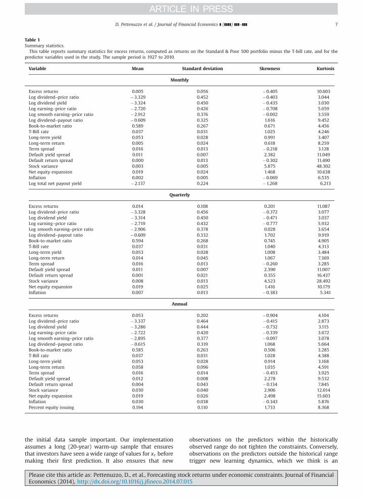
Table 1Summary statistics.
This table reports summary statistics for excess returns, computed as returns on the Standard & Poor 500 portfolio minus the T-bill rate, and for thepredictor variables used in the study. The sample period is 1927 to 2010.
Variable Mean Standard deviation Skewness Kurtosis
Monthly
Excess returns 0.005 0.056 �0.405 10.603Log dividend–price ratio �3.329 0.452 �0.403 3.044Log dividend yield �3.324 0.450 �0.435 3.030Log earning–price ratio �2.720 0.426 �0.708 5.659Log smooth earning–price ratio �2.912 0.376 �0.002 3.559Log dividend–payout ratio �0.609 0.325 1.616 9.452Book-to-market ratio 0.589 0.267 0.671 4.456T-Bill rate 0.037 0.031 1.025 4.246Long-term yield 0.053 0.028 0.991 3.407Long-term return 0.005 0.024 0.618 8.259Term spread 0.016 0.013 �0.218 3.128Default yield spread 0.011 0.007 2.382 11.049Default return spread 0.000 0.013 �0.302 11.490Stock variance 0.003 0.005 5.875 48.302Net equity expansion 0.019 0.024 1.468 10.638Inflation 0.002 0.005 �0.069 6.535Log total net payout yield �2.137 0.224 �1.268 6.213
Quarterly
Excess returns 0.014 0.108 0.201 11.087Log dividend–price ratio �3.328 0.456 �0.372 3.077Log dividend yield �3.314 0.450 �0.471 3.037Log earning–price ratio �2.719 0.432 �0.777 5.932Log smooth earning–price ratio �2.906 0.378 0.028 3.654Log dividend–payout ratio �0.609 0.332 1.702 9.919Book-to-market ratio 0.594 0.268 0.745 4.905T-Bill rate 0.037 0.031 1.040 4.313Long-term yield 0.053 0.028 1.008 3.484Long-term return 0.014 0.045 1.067 7.369Term spread 0.016 0.013 �0.260 3.285Default yield spread 0.011 0.007 2.390 11.007Default return spread 0.001 0.021 0.355 16.437Stock variance 0.008 0.013 4.523 28.492Net equity expansion 0.019 0.025 1.416 10.179Inflation 0.007 0.013 �0.383 5.341
Annual
Excess returns 0.053 0.202 �0.904 4.104Log dividend–price ratio �3.337 0.464 �0.415 2.873Log dividend yield �3.286 0.444 �0.732 3.115Log earning–price ratio �2.722 0.420 �0.339 3.672Log smooth earning–price ratio �2.895 0.377 �0.097 3.078Log dividend–payout ratio �0.615 0.319 1.068 5.664Book-to-market ratio 0.585 0.263 0.506 3.285T-Bill rate 0.037 0.031 1.028 4.388Long-term yield 0.053 0.028 0.914 3.168Long-term return 0.058 0.096 1.035 4.591Term spread 0.016 0.014 �0.453 3.925Default yield spread 0.012 0.008 2.278 9.532Default return spread 0.004 0.043 �0.134 7.845Stock variance 0.030 0.040 2.906 12.014Net equity expansion 0.019 0.026 2.498 15.603Inflation 0.030 0.038 �0.343 5.876Percent equity issuing 0.194 0.110 1.733 8.368
D. Pettenuzzo et al. / Journal of Financial Economics ] (]]]]) ]]]–]]] 7
the initial data sample important. Our implementationassumes a long (20-year) warm-up sample that ensuresthat investors have seen a wide range of values for xτ beforemaking their first prediction. It also ensures that new
Please cite this article as: Pettenuzzo, D., et al., Forecasting stocEconomics (2014), http://dx.doi.org/10.1016/j.jfineco.2014.07.01
observations on the predictors within the historicallyobserved range do not tighten the constraints. Conversely,observations on the predictors outside the historical rangetrigger new learning dynamics, which we think is an
k returns under economic constraints. Journal of Financial5i

−0.01 −0.005 0 0.005 0.01 0.015 0.02 0.0250
50
100
150
200
250
−0.4 −0.3 −0.2 −0.1 0 0.1 0.2 0.30
5
10
15
−1 −0.5 0 0.5 1 1.50
0.5
1
1.5
2
2.5
Log dividend−price ratio
T−Bill rate
Default yield spread
Fig. 4. Slope coefficient of predictors under constrained and unconstrained models. This figure shows the posterior density of the slope coefficient, β, froma regression of monthly excess returns ðrtþ1Þ on an intercept and a lagged predictor variable, xt: rtþ1 ¼ μþβxtþεtþ1. The equity premium constrainedmodel imposes that r̂ τþ1jt ¼
R ðμþβxτÞpðμ; βjDt Þ dμ dβ40; for τ¼ 1;…; t and information set Dt , and the Sharpe ratio constraint imposes that0r r̂ τþ1jt=σ̂ τþ1jtr1, for τ¼ 1;…; t, where σ̂ τþ1jt is the posterior volatility estimate obtained from a stochastic volatility model. The posterior densityestimates shown here are based on the full sample at the end of 2010. Panels A, B, and C use the log dividend–price ratio, T-bill rate, and the default yieldspread as the predictor, respectively.
D. Pettenuzzo et al. / Journal of Financial Economics ] (]]]]) ]]]–]]]8
attractive feature of our setup. Moreover, we condition onthe predictor variables, treating them as exogenous insteadof as part of the data being modeled.
2.1.2. Sharpe ratio constraintIn this subsection, we explore a novel way of sharpen-
ing the forecasts of excess market returns, namely, byplacing constraints on the conditional Sharpe ratio of themarket portfolio. Such constraints could be motivatedfrom an asset pricing perspective, as the Sharpe ratio isfrequently used in the calibration and evaluation of struc-tural asset pricing models.10 For US data, the Sharpe ratiohas been found to be time-varying and countercyclical(Brandt, 2010; Lettau and Ludvigson, 2010). More impor-tant, the empirical Sharpe ratio appears more volatile thanwhat the leading asset pricing models would suggest. Thisempirical fact has been labeled the “Sharpe ratio varia-bility puzzle” by Lettau and Ludvigson (2010). Naturally,the Sharpe ratio is most often used for portfolio perfor-mance evaluation [see Brandt, 2010 for a review article].
10 See Cochrane (2001) for a textbook treatment of the Sharpe ratio'suse in evaluating asset pricing models. Lettau and Ludvigson (2010)review whether some leading asset pricing models can replicate thestylized facts regarding the Sharpe ratio in the US. Lettau and Wachter(2007, 2011) use the Sharpe ratio in the calibration of their assetpricing model.
Please cite this article as: Pettenuzzo, D., et al., Forecasting stocEconomics (2014), http://dx.doi.org/10.1016/j.jfineco.2014.07.01
Given all the theoretical and empirical work on thissubject, most academics and practitioners are likely tohave some priors about what constitutes a reasonableSharpe ratio.
The conditional Sharpe ratio depends on both theconditional mean and volatility of the return distribution.Because time variation in volatility is a well-documentedfact in empirical finance (see, e.g., Andersen, Bollerslev,Christoffersen, and Diebold, 2006), we modify Eq. (1):
rτþ1 ¼ μþβxτþexpðhτþ1Þuτþ1; ð5Þwhere hτþ1 denotes the (log of) return volatility at timeτþ1 and uτþ1 �Nð0;1Þ. Following common stochasticvolatility models, log volatility is assumed to evolve as adriftless random walk,
hτþ1 ¼ hτþξτþ1; ð6Þwhere ξτþ1 �Nð0;σ2
ξÞ and uτ and ξs are mutually inde-pendent for all τ and s.
Next, define the (approximate) annualized conditionalSharpe ratio at time τ as
SRτþ1jτ ¼ffiffiffiffiH
pðμþβxτÞ
expðhτþ0:5σ2ξÞ; ð7Þ
where H denotes the number of observations per year (i.e.,H¼ 12, 4; and 1 with monthly, quarterly, and annual data,respectively). We assume that the conditional Sharpe ratio
k returns under economic constraints. Journal of Financial5i
−0.015 −0.01 −0.005 0 0.005 0.01 0.015 0.02 0.025 0.030
100
200
300mean
−0.015 −0.01 −0.005 0 0.005 0.01 0.015 0.02 0.025 0.030
100
200
300mean − 2 standard deviations
−0.015 −0.01 −0.005 0 0.005 0.01 0.015 0.02 0.025 0.030
100
200
300mean + 2 standard deviations
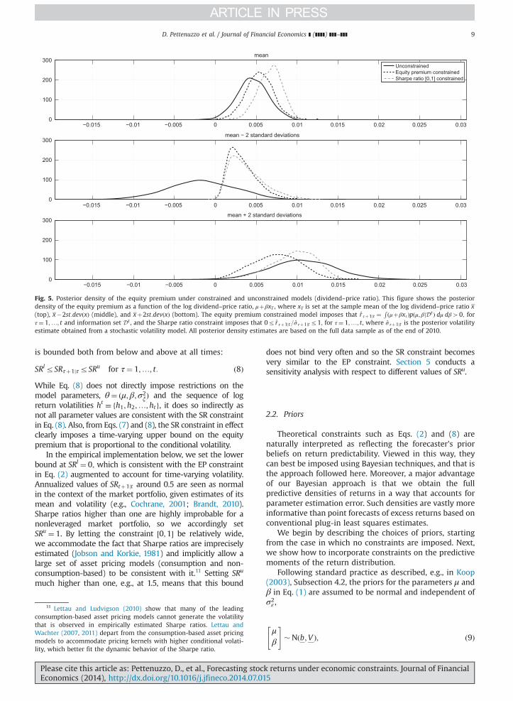
Fig. 5. Posterior density of the equity premium under constrained and unconstrained models (dividend–price ratio). This figure shows the posteriordensity of the equity premium as a function of the log dividend–price ratio, μþβxT , where xT is set at the sample mean of the log dividend–price ratio x(top), x�2st:devðxÞ (middle), and xþ2st:devðxÞ (bottom). The equity premium constrained model imposes that r̂ τþ1jt ¼
R ðμþβxτÞpðμ; βjDt Þ dμ dβ40; forτ¼ 1;…; t and information set Dt , and the Sharpe ratio constraint imposes that 0r r̂ τþ1jt=σ̂ τþ1jtr1; for τ¼ 1;…; t, where σ̂ τþ1jt is the posterior volatilityestimate obtained from a stochastic volatility model. All posterior density estimates are based on the full data sample as of the end of 2010.
D. Pettenuzzo et al. / Journal of Financial Economics ] (]]]]) ]]]–]]] 9
is bounded both from below and above at all times:
SRlrSRτþ1jτrSRu for τ¼ 1;…; t: ð8Þ
While Eq. (8) does not directly impose restrictions on themodel parameters, θ¼ ðμ;β;σ2
ξÞ and the sequence of logreturn volatilities ht � fh1;h2;…;htg, it does so indirectly asnot all parameter values are consistent with the SR constraintin Eq. (8). Also, from Eqs. (7) and (8), the SR constraint in effectclearly imposes a time-varying upper bound on the equitypremium that is proportional to the conditional volatility.
In the empirical implementation below, we set the lowerbound at SRl ¼ 0; which is consistent with the EP constraintin Eq. (2) augmented to account for time-varying volatility.Annualized values of SRtþ1jt around 0.5 are seen as normalin the context of the market portfolio, given estimates of itsmean and volatility (e.g., Cochrane, 2001; Brandt, 2010).Sharpe ratios higher than one are highly improbable for anonleveraged market portfolio, so we accordingly setSRu ¼ 1. By letting the constraint ½0;1� be relatively wide,we accommodate the fact that Sharpe ratios are impreciselyestimated (Jobson and Korkie, 1981) and implicitly allow alarge set of asset pricing models (consumption and non-consumption-based) to be consistent with it.11 Setting SRu
much higher than one, e.g., at 1.5, means that this bound
11 Lettau and Ludvigson (2010) show that many of the leadingconsumption-based asset pricing models cannot generate the volatilitythat is observed in empirically estimated Sharpe ratios. Lettau andWachter (2007, 2011) depart from the consumption-based asset pricingmodels to accommodate pricing kernels with higher conditional volati-lity, which better fit the dynamic behavior of the Sharpe ratio.
Please cite this article as: Pettenuzzo, D., et al., Forecasting stocEconomics (2014), http://dx.doi.org/10.1016/j.jfineco.2014.07.01
does not bind very often and so the SR constraint becomesvery similar to the EP constraint. Section 5 conducts asensitivity analysis with respect to different values of SRu.
2.2. Priors
Theoretical constraints such as Eqs. (2) and (8) arenaturally interpreted as reflecting the forecaster's priorbeliefs on return predictability. Viewed in this way, theycan best be imposed using Bayesian techniques, and that isthe approach followed here. Moreover, a major advantageof our Bayesian approach is that we obtain the fullpredictive densities of returns in a way that accounts forparameter estimation error. Such densities are vastly moreinformative than point forecasts of excess returns based onconventional plug-in least squares estimates.
We begin by describing the choices of priors, startingfrom the case in which no constraints are imposed. Next,we show how to incorporate constraints on the predictivemoments of the return distribution.
Following standard practice as described, e.g., in Koop(2003), Subsection 4.2, the priors for the parameters μ andβ in Eq. (1) are assumed to be normal and independent ofσ2ε ,
μβ
" #�Nðb;V Þ; ð9Þ
k returns under economic constraints. Journal of Financial5i
−0.02 −0.015 −0.01 −0.005 0 0.005 0.01 0.015 0.02 0.025 0.030
100
200
300mean
−0.02 −0.015 −0.01 −0.005 0 0.005 0.01 0.015 0.02 0.025 0.030
100
200
300mean − 2 standard deviations
−0.02 −0.015 −0.01 −0.005 0 0.005 0.01 0.015 0.02 0.025 0.030
100
200
300mean + 2 standard deviations
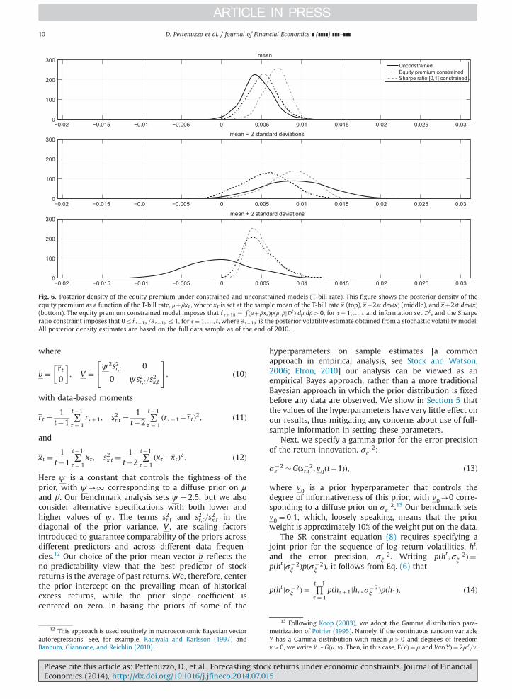
Fig. 6. Posterior density of the equity premium under constrained and unconstrained models (T-bill rate). This figure shows the posterior density of theequity premium as a function of the T-bill rate, μþβxT , where xT is set at the sample mean of the T-bill rate x (top), x�2st:devðxÞ (middle), and xþ2st:devðxÞ(bottom). The equity premium constrained model imposes that r̂ τþ1jt ¼
R ðμþβxτÞpðμ; βjDt Þ dμ dβ40; for τ¼ 1;…; t and information set Dt , and the Sharperatio constraint imposes that 0r r̂ τþ1jt=σ̂ τþ1jtr1; for τ¼ 1;…; t, where σ̂ τþ1jt is the posterior volatility estimate obtained from a stochastic volatility model.All posterior density estimates are based on the full data sample as of the end of 2010.
D. Pettenuzzo et al. / Journal of Financial Economics ] (]]]]) ]]]–]]]10
where
b ¼ rt0
� �; V ¼
ψ 2s2r;t 0
0 ψ s2r;t=s2x;t
24 35; ð10Þ
with data-based moments
rt ¼1
t�1∑t�1
τ ¼ 1rτþ1; s2r;t ¼
1t�2
∑t�1
τ ¼ 1ðrτþ1�rtÞ2; ð11Þ
and
xt ¼1
t�1∑t�1
τ ¼ 1xτ ; s2x;t ¼
1t�2
∑t�1
τ ¼ 1ðxτ�xtÞ2: ð12Þ
Here ψ is a constant that controls the tightness of theprior, with ψ-1 corresponding to a diffuse prior on μand β. Our benchmark analysis sets ψ ¼ 2:5; but we alsoconsider alternative specifications with both lower andhigher values of ψ . The terms s2r;t and s2r;t=s
2x;t in the
diagonal of the prior variance, V , are scaling factorsintroduced to guarantee comparability of the priors acrossdifferent predictors and across different data frequen-cies.12 Our choice of the prior mean vector b reflects theno-predictability view that the best predictor of stockreturns is the average of past returns. We, therefore, centerthe prior intercept on the prevailing mean of historicalexcess returns, while the prior slope coefficient iscentered on zero. In basing the priors of some of the
12 This approach is used routinely in macroeconomic Bayesian vectorautoregressions. See, for example, Kadiyala and Karlsson (1997) andBanbura, Giannone, and Reichlin (2010).
Please cite this article as: Pettenuzzo, D., et al., Forecasting stocEconomics (2014), http://dx.doi.org/10.1016/j.jfineco.2014.07.01
hyperparameters on sample estimates [a commonapproach in empirical analysis, see Stock and Watson,2006; Efron, 2010] our analysis can be viewed as anempirical Bayes approach, rather than a more traditionalBayesian approach in which the prior distribution is fixedbefore any data are observed. We show in Section 5 thatthe values of the hyperparameters have very little effect onour results, thus mitigating any concerns about use of full-sample information in setting these parameters.
Next, we specify a gamma prior for the error precisionof the return innovation, σ�2
ε :
σ�2ε � Gðs�2
r;t ; v0ðt�1ÞÞ; ð13Þ
where v0 is a prior hyperparameter that controls thedegree of informativeness of this prior, with v0-0 corre-sponding to a diffuse prior on σ�2
ε .13 Our benchmark setsv0 ¼ 0:1; which, loosely speaking, means that the priorweight is approximately 10% of the weight put on the data.
The SR constraint equation (8) requires specifying ajoint prior for the sequence of log return volatilities, ht,and the error precision, σ�2
ξ . Writing pðht ;σ�2ξ Þ ¼
pðht jσ�2ξ Þpðσ�2
ξ Þ, it follows from Eq. (6) that
pðht jσ�2ξ Þ ¼ ∏
t�1
τ ¼ 1pðhτþ1jhτ ;σ�2
ξ Þpðh1Þ; ð14Þ
13 Following Koop (2003), we adopt the Gamma distribution para-metrization of Poirier (1995). Namely, if the continuous random variableY has a Gamma distribution with mean μ40 and degrees of freedomv40, we write Y � Gðμ; vÞ: Then, in this case, EðYÞ ¼ μ and VarðYÞ ¼ 2μ2=v.
k returns under economic constraints. Journal of Financial5i

−0.015 −0.01 −0.005 0 0.005 0.01 0.015 0.02 0.0250
50
100
150
200
250mean
−0.015 −0.01 −0.005 0 0.005 0.01 0.015 0.02 0.0250
50
100
150
200
250mean − 2 standard deviations
−0.015 −0.01 −0.005 0 0.005 0.01 0.015 0.02 0.0250
50
100
150
200
250mean + 2 standard deviations
Fig. 7. Posterior density of the equity premium under constrained and unconstrained models (default spread). This figure shows the posterior density ofthe equity premium as a function of the default yield spread, μþβxT , where xT is set at the sample mean of the default yield spread x (top), x�2st:devðxÞ(middle), and xþ2st:devðxÞ (bottom). The equity premium constrained model imposes that r̂ τþ1jt ¼
R ðμþβxτÞpðμ; βjDt Þ dμ dβ40; for τ¼ 1;…; t andinformation set Dt , and the Sharpe ratio constraint imposes that 0r r̂ τþ1jt=σ̂ τþ1jtr1; for τ¼ 1;…; t, where σ̂ τþ1jt is the posterior volatility estimateobtained from a stochastic volatility model. All posterior density estimates are based on the full data sample as of the end of 2010.
D. Pettenuzzo et al. / Journal of Financial Economics ] (]]]]) ]]]–]]] 11
with hτþ1jhτ ;σ�2ξ �Nðhτ ;σ2
ξÞ: Thus, to complete the priorelicitation for pðht ;σ�2
ξ Þ; we need to specify priors only forh1, the initial log volatility, and σ�2
ξ . We choose these fromthe normal-gamma family as follows:
h1 �Nðlnðsr;tÞ; khÞ ð15Þ
and
σ�2ξ � Gð1=kξ;1Þ: ð16Þ
We set kξ ¼ 0:01 and choose the remaining hyperpara-meters in Eqs. (15) and (16) to imply uninformative priors,allowing the data to determine the degree of time varia-tion in the return volatility. Accordingly, we specifykh ¼ 10, and set the degrees of freedom for σ�2
ξ to 1.Section 5 discusses robustness of our results with respectto changes in the priors.
2.3. Imposing economic constraints
We next describe how we impose the economic con-straints on the model parameters. Starting with the EPconstraint, we modify the priors on μ and β in Eq. (9) to
μβ
" #�Nðb;V Þ; μ;βAAt ; ð17Þ
where At is a set such that
At ¼ fμþβxτZ0; τ¼ 1;…; tg: ð18Þ
Please cite this article as: Pettenuzzo, D., et al., Forecasting stocEconomics (2014), http://dx.doi.org/10.1016/j.jfineco.2014.07.01
Similarly, for the SR constraint, we restrict the priors onfμ;β;σ�2
ξ ;h1;h2;…;htgA ~At , where ~At is a set satisfying
~At ¼ fSRlrSRτþ1jτrSRu; τ¼ 1;…; tg; ð19Þand SRτþ1jτ is given in Eq. (7).
The Appendix provides details of how we estimate theparameters and compute forecasts for the unconstrainedand constrained models.
As a final point about the above analysis, we note thatthe boundaries of the constraints in Eqs. (2) and (8) areconstants (0, SRl; and SRu), motivated by economic con-siderations. However, one could view the boundariesthemselves as being parameters with associated priors.In that case, our specification corresponds to havingdogmatic priors on these specific parameters. This general-ization could be less meaningful for constraints that arereadily imposed by economic theory (such as the zerolower bound on the equity premium and Sharpe ratio)than for others (such as the upper bound on the Sharperatio). From an econometric perspective, updating priorsabout the boundary parameters is nontrivial. Given thatthe benefits of such a generalization are not clear, whilethe tractability and computational costs of imposing it aresubstantial, we conduct our empirical analysis by imposingthe constraints in Eqs. (2) and (8) as discussed above.
3. Empirical results
This section presents data and empirical results usingthe methods for incorporating economic constraintsdescribed in Section 2 to predict the equity premium.
k returns under economic constraints. Journal of Financial5i
Exc
ess
retu
rn fo
reca
sts
Log dividend−price ratio
1940 1945 1950 1955 1960 1965 1970 1975 1980 1985 1990 1995 2000 2005
0
5
10
x 10−3
Exc
ess
retu
rn fo
reca
sts
T−Bill rate
1940 1945 1950 1955 1960 1965 1970 1975 1980 1985 1990 1995 2000 2005
−0.015−0.01−0.00500.0050.01
Exc
ess
retu
rn fo
reca
sts
Default yield spread
1940 1945 1950 1955 1960 1965 1970 1975 1980 1985 1990 1995 2000 2005
0246810
x 10−3
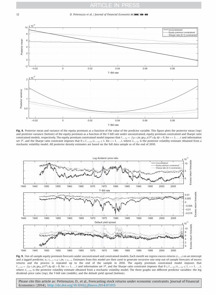
Fig. 9. Out-of-sample equity premium forecasts under unconstrained and constrained models. Each month we regress excess returns ðrtþ1Þ on an interceptand a lagged predictor, xt: rtþ1 ¼ μþβxtþεtþ1. Estimates from this model are then used to generate recursive one-step out-of-sample forecasts of excessreturns and the process is repeated up to the end of the sample in 2010. The equity premium constrained model imposes thatr̂ τþ1jt ¼
R ðμþβxτÞpðμ; βjDt Þ dμ dβ40; for τ¼ 1;…; t and information set Dt , and the Sharpe ratio constraint imposes that 0r r̂ τþ1jt=σ̂ τþ1jtr1, τ¼ 1;…; t,where σ̂ τþ1jt is the posterior volatility estimate obtained from a stochastic volatility model. The three graphs use different predictor variables: the logdividend–price ratio (top), the T-bill rate (middle), and the default yield spread (bottom).
−0.02 0 0.02 0.04 0.06 0.08−2
0
2
4
6
8
10 x 10−3
T−Bill rate
Pos
terio
r mea
n
−0.02 0 0.02 0.04 0.06 0.080
0.5
1
1.5
2 x 10⁻⁵
T−Bill rate
Pos
terio
r var
ianc
e
Fig. 8. Posterior mean and variance of the equity premium as a function of the value of the predictor variable. This figure plots the posterior mean (top)and posterior variance (bottom) of the equity premium as a function of the T-bill rate under unconstrained, equity premium constrained and Sharpe ratioconstrained models, respectively. The equity premium constrained model imposes that r̂ τþ1jt ¼
R ðμþβxτÞpðμ; βjDt Þ dμ dβ40; for τ¼ 1;…; t and informationset Dt , and the Sharpe ratio constraint imposes that 0r r̂ τþ1jt=σ̂ τþ1jtr1; for τ¼ 1;…; t, where σ̂ τþ1jt is the posterior volatility estimate obtained from astochastic volatility model. All posterior density estimates are based on the full data sample as of the end of 2010.
Please cite this article as: Pettenuzzo, D., et al., Forecasting stock returns under economic constraints. Journal of FinancialEconomics (2014), http://dx.doi.org/10.1016/j.jfineco.2014.07.015i
D. Pettenuzzo et al. / Journal of Financial Economics ] (]]]]) ]]]–]]]12

D. Pettenuzzo et al. / Journal of Financial Economics ] (]]]]) ]]]–]]] 13
3.1. Data
Our empirical analysis uses data on stock returns alongwith a set of 17 predictor variables originally analyzed inWelch and Goyal (2008) and subsequently extended up to
1940 1945 1950 1955 1960 1965 1970 1975
Fig. 10. Volatility forecasts. This figure shows the one-step-ahead recursivedistribution based on the stochastic volatility model that uses the log dihtþ1 ¼ htþξtþ1.
Log dividend−pric
1935 1940 1945 1950 1955 1960 1965 1970 1975
T−Bill rate
1935 1940 1945 1950 1955 1960 1965 1970 1975
Default yield spr
1935 1940 1945 1950 1955 1960 1965 1970 1975
Fig. 11. Conditional Sharpe ratios. This figure shows the time series of conditiobased on the unconstrained, equity premium constrained, and Sharpe ratio conststochastic volatility (SV)]. The three graphs use different predictor variables: the lspread (bottom).
Please cite this article as: Pettenuzzo, D., et al., Forecasting stocEconomics (2014), http://dx.doi.org/10.1016/j.jfineco.2014.07.01
2010 by the same authors. Stock returns are computedfrom the Standard and Poor's (S&P) 500 index and includedividends. A short T-bill rate is subtracted from stockreturns to capture excess returns. Data samples varyconsiderably across the individual predictor variables. To
Exc
ess
retu
rn v
olat
ility
1980 1985 1990 1995 2000 20050
0.05
0.1
conditional volatility forecasts computed from the predictive returnvidend–price ratio as predictor, rtþ1 ¼ μþβ logðDt=Pt Þþexpðhtþ1Þutþ1,
Ann
ualiz
ed S
harp
e ra
tio
e ratio
1980 1985 1990 1995 2000 2005
0
0.5
1
Ann
ualiz
ed S
harp
e ra
tio
1980 1985 1990 1995 2000 2005−1
−0.5
0
0.5
1
Ann
ualiz
ed S
harp
e ra
tio
ead
1980 1985 1990 1995 2000 2005
0
0.5
1
nal Sharpe ratios computed from the predictive density of excess returnsrained models [the last computed under both constant volatility (CV) andog dividend–price ratio (top), the T-bill rate (middle), and the default yield
k returns under economic constraints. Journal of Financial5i

1965 1970 1975 1980
0.01
0.02
0.03
0.04
0.05
Unconstrained μ
1965 1970 1975 1980
0.01
0.02
0.03
0.04
0.05
Equity premium constrained μ
1965 1970 1975 1980
−1
−0.8
−0.6
−0.4
−0.2
0
Unconstrained β
1965 1970 1975 1980
−1
−0.8
−0.6
−0.4
−0.2
0
Equity premium constrained β
Fig. 12. Posterior probability intervals for the parameters of the return prediction model. Each month we update the posterior density of the parametersμ; β of the return prediction model rtþ1 ¼ μþβxtþεtþ1 ; where xt is the T-bill rate and rtþ1 is the return on the Standard & Poor 500 index, measured inexcess of the T-bill rate. We then compute posterior probability intervals for these parameter estimates. Left-hand graphs report the ð2:5;97:5Þ percentileposterior probability intervals for the parameters of the unconstrained model, and right-hand graphs show results for the equity-premium constrainedmodel. The equity premium constrained model imposes that r̂ τþ1jt ¼
R ðμþβxτÞpðμ; βjDt Þ dμ dβ40 for all τ¼ 1;…; t and information set Dt . All densityestimates are updated recursively through time.
D. Pettenuzzo et al. / Journal of Financial Economics ] (]]]]) ]]]–]]]14
be able to compare results across the individual predictorvariables, we use the longest common sample, that is,1927–2010. In addition, we use the first 20 years of data asa training sample. For example, for the monthly data weinitially estimate our regression models over the periodJanuary 1927–December 1946, and we use the estimatedcoefficients to forecast excess returns for January 1947.We next include January 1947 in the estimation sample,which becomes January 1927–January 1947, and we usethe corresponding estimates to predict excess returns forFebruary 1947. We proceed in this recursive fashion untilthe last observation in the sample, thus producing a timeseries of one-step-ahead forecasts spanning the timeperiod from January 1947 to December 2010.
The identity of the predictor variables, along withsummary statistics, is provided in Table 1. Most variablesfall into three broad categories: (1) valuation ratios captur-ing some measure of fundamentals to market value suchas the dividend price ratio, the dividend yield, the earn-ings–price ratio, the ten-year earnings–price ratio, or thebook-to-market ratio; (2) measures of bond yields captur-ing level effects (the three-month T-bill rate and the yieldon long term government bonds), slope effects (the termspread), and default risk effects (the default yield spreaddefined as the yield spread between BAA- and AAA-ratedcorporate bonds, and the default return spread defined asthe difference between the yield on long-term corporateand government bonds); and (3) estimates of equityrisk such as the long-term return and stock variance(a volatility estimate based on daily squared returns).
Please cite this article as: Pettenuzzo, D., et al., Forecasting stocEconomics (2014), http://dx.doi.org/10.1016/j.jfineco.2014.07.01
Furthermore, three corporate finance variables are con-sidered, namely, the dividend payout ratio (the log of thedividend-earnings ratio), net equity expansion (the ratio of12-month net issues by NYSE-listed stocks over the year-end market capitalization), and percent equity issuing (theratio of equity issuing activity as a fraction of total issuingactivity) as well as a macroeconomic variable, inflation(the rate of change in the consumer price index). Wefollow Welch and Goyal (2008) and, for monthly andquarterly data, lag inflation an extra period to accountfor the delay in releases of the consumer price index.
To make our results comparable to studies from theliterature on return predictability such as Campbell andThompson (2008) and Welch and Goyal (2008), we focuson univariate regressions with a single predictor variable.However, we also consider how our approach can beextended to incorporate multivariate information (seeSection 5). Finally, because there are too many variablesto cover in detail, we focus our analysis on three pre-dictors: the log dividend–price ratio, the T-bill rate, andthe default yield spread, all of which have featuredprominently in the literature on return predictability.
3.2. Coefficient estimates and predictive densities
As shown in Figs. 1–3, the economic constraints on thepredictive moments of the return distribution affect theparameter estimates in a way that reflects the entire sequenceof data points. This gives rise to parameter estimates that arevery different from the standard, unconstrained ones typically
k returns under economic constraints. Journal of Financial5i

Table 2Out-of-sample forecast performance (monthly).
This table reports the out-of-sample R2 of unconstrained and constrained univariate prediction models for the monthly excess return, rtþ1, measured relative to the prevailing mean model:
R2OoS ¼ 1�
∑t �1τ ¼ t �1ðrtþ1� r̂ tþ1jt Þ2
∑t �1τ ¼ t �1ðrtþ1�r tþ1jt Þ2
;
where r̂ tþ1jt is the mean of the predictive return distribution based on a regression of monthly excess returns on an intercept and a lagged predictor variable, xt: rtþ1 ¼ μþβxtþεtþ1. r tþ1jt is the forecast from the
prevailing mean model, which assumes that β¼ 0. The Campbell and Thompson (CT) truncation approach sets r̂ tþ1jt ¼maxð0; μ̂ tþ β̂ txt Þ, where μ̂t and β̂ t are the time t ordinary least squares estimates of μ and β.The equity premium (EP) constrained model imposes that r̂ τþ1jt ¼
R ðμþβxτÞpðμ; βjDt Þ dμ dβ40; for τ¼ 1;…; t and information set Dt , and the Sharpe ratio (SR [0,1]) constraint imposes that 0r r̂ τþ1jt=σ̂ τþ1jtr1, forτ¼ 1;…; t, where σ̂ τþ1jt is the posterior volatility estimate obtained from a stochastic volatility model. Panel A shows results for the full sample (1947–2010), while panels B and C report results for the subsamples1947–1978 and 1979–2010. Also reported are averages across all predictor variables. Bold figures highlight instances in which the constrained ROoS
2is higher than its unconstrained counterpart. We measure
statistical significance relative to the prevailing mean model using the Clark and West (2007) test statistic. nsignificance at 10% level; nnsignificance at 5% level; nnnsignificance at 1% level.
Panel A: full sample (1947–2010) Panel B: 1947–1978 Panel C: 1979–2010
Variable No CT EP SR [0,1] No CT EP SR [0,1] No CT EP SR [0,1]constraint truncation constraint constraint constraint truncation constraint constraint constraint truncation constraint constraint
Log dividend–price ratio 0.10%n 0.25%nn 0.64%nnn 0.49%nn 1.01%nn 1.01%nn 1.31%nnn 1.03%nn �0.59% �0.33% 0.14% 0.08%Log dividend yield �0.16%nn 0.31%nn 0.76%nnn 0.54%nn 0.97%nnn 1.18%nnn 1.55%nnn 1.05%nn �1.01% �0.35% 0.17% 0.16%Log earning–price ratio �1.38%n �0.45%nn 0.25%n 0.30%n �1.17%n �0.80%n 0.18% 0.43% �1.54% �0.19% 0.31% 0.20%Log smooth earning–price ratio �0.79%n 0.07%nn 0.48%nn 0.47%nn �0.14%n 0.26%n 0.81%nn 0.94%nn �1.28% �0.07% 0.23% 0.12%Log dividend–payout ratio �1.57% �1.29% �0.12% 0.03% �2.64% �2.64% �0.32% 0.23% �0.76% �0.26% 0.03% �0.12%Book-to-market ratio �1.40% �0.88% 0.02% 0.04% �0.42% �0.49% 0.08% 0.06% �2.14% �1.17% �0.03% 0.02%T-Bill rate 0.01%n 0.20%n 0.10% 0.54%nn 1.50%nn 1.21%nn 0.28% 1.40%nnn �1.11% �0.57% �0.04% �0.11%Long-term yield �0.94%n 0.20%nn 0.31%nn 0.55%nnn �0.47%n 1.02%nn 0.78%nn 1.43%nnn �1.30% �0.42% �0.04% �0.11%Long-term return �0.74% �0.62% 0.19% 0.53%nn �1.90% �1.61% 0.31% 1.25%nn 0.13% 0.13% 0.10% �0.02%Term spread 0.06% 0.04% 0.05% 0.24%n 0.41% 0.41% 0.14% 0.53%n �0.20% �0.23% �0.02% 0.02%Default yield spread �0.19% �0.18% 0.18% �0.08% �0.24% �0.22% 0.53%nn 0.22% �0.15% �0.15% �0.07% �0.31%Default return spread �0.24% �0.39% 0.15% �0.30% �0.97% �0.97% 0.37% �0.42% 0.32% 0.05% 0.00% �0.20%Stock variance 0.24% 0.11% �0.17% �0.29% �0.07% �0.07% 0.36%n 0.08% 0.48% 0.24% �0.57% �0.56%Net equity expansion �0.79% �0.77% �0.01% �0.08% 0.08% 0.12% 0.15% 0.03% �1.45% �1.44% �0.13% �0.16%Inflation �0.13% �0.13% 0.07% �0.12% �0.05% �0.05% 0.14% 0.36% �0.20% �0.20% 0.02% �0.47%Log total net payout yield �0.49%n 0.09%n 0.18% �0.01% 1.44%nnn 1.21%nn 0.45%n 0.25% �1.97% �0.76% 0.00% �0.17%
Average �0.53% �0.22% 0.19% 0.18% �0.17% �0.03% 0.44% 0.55% �0.80% �0.36% 0.01% �0.10%
Pleasecite
thisarticle
as:Petten
uzzo,D
.,etal.,Forecastin
gstock
return
sunder
econom
iccon
straints.Jou
rnalofFin
ancial
Econom
ics(2014),h
ttp://d
x.doi.org/10.1016/j.jfin
eco.2014.07.015i
D.Pettenuzzo
etal./
Journalof
FinancialEconom
ics](]]]])
]]]–]]]
15

Table 3Out-of-sample forecast performance (quarterly).
This table reports the out-of-sample R2 of unconstrained and constrained univariate prediction models for the quarterly excess return, rtþ1, measured relative to the prevailing mean model:
R2OoS ¼ 1�
∑t �1τ ¼ t �1ðrtþ1� r̂ tþ1jt Þ2
∑t �1τ ¼ t �1ðrtþ1�r tþ1jt Þ2
;
where r̂ tþ1jt is the mean of the predictive return distribution based on a regression of monthly excess returns on an intercept and a lagged predictor variable, xt: rtþ1 ¼ μþβxtþεtþ1. r tþ1jt is the forecast from the
prevailing mean model, which assumes that β¼ 0. The Campbell and Thompson (CT) truncation approach sets r̂ tþ1jt ¼maxð0; μ̂ tþ β̂ txt Þ, where μ̂t and β̂ t are the time t ordinary least squares estimates of μ and β.The equity premium (EP) constrained model imposes that r̂ τþ1jt ¼
R ðμþβxτÞpðμ; βjDt Þ dμ dβ40; for τ¼ 1;…; t and information set Dt , and the Sharpe ratio (SR [0,1]) constraint imposes that 0r r̂ τþ1jt=σ̂ τþ1jtr1; forτ¼ 1;…; t, where σ̂ τþ1jt is the posterior volatility estimate obtained from a stochastic volatility model. Panel A shows results for the full sample (1947–2010), while panels B and C report results for the subsamples1947–1978 and 1979–2010. Also reported are averages across all predictor variables. Bold figures highlight instances in which the constrained ROoS
2is higher than its unconstrained counterpart. We measure
statistical significance relative to the prevailing mean model using the Clark and West (2007) test statistic. nsignificance at 10% level; nnsignificance at 5% level; nnnsignificance at 1% level.
Panel A: full sample (1947–2010) Panel B: 1947–1978 Panel C: 1979–2010
Variable No CT EP SR [0,1] No CT EP SR [0,1] No CT EP SR [0,1]constraint truncation constraint constraint constraint truncation constraint constraint constraint truncation constraint constraint
Log dividend–price ratio �0.16%nn 1.20%nn 2.11%nnn 1.68%nnn 3.22%nnn 3.72%nnn 4.27%nnn 3.07%nnn �3.10% �0.98% 0.24% 0.47%Log dividend yield 0.75%nn 1.86%nn 2.04%nnn 1.88%nnn 4.19%nnn 4.18%nnn 4.04%nnn 3.38%nnn �2.22% �0.14% 0.32% 0.57%Log earning–price ratio �6.33%n �2.42%nn 0.70%nn 0.92%nn �4.65%nn �3.37%nn 0.78%n 1.60%nn �7.78% �1.60% 0.63% 0.33%Log smooth earning–price ratio �3.58%nn 0.50%nn 1.57%nn 1.60%nn �0.80%nn 1.77%nn 3.03%nn 2.96%nnn �5.98% �0.60% 0.30% 0.41%Log dividend–payout ratio �3.69% �3.02% 0.04% 0.81%nn �5.16% �5.16% �0.04% 1.75%nnn �2.42% �1.17% 0.11% 0.00%Book-to-market ratio �6.24% �3.16% �0.15% 0.96%n �1.64% �1.22% 0.04% 1.64%n �10.23% �4.84% �0.32% 0.37%T-Bill rate �0.53% 0.47% 0.01% 1.87%nnn 2.40% 2.92%nn 0.34% 3.87%nnn �3.06% �1.65% �0.27% 0.14%Long-term yield �2.70% 0.39%n 0.61%n 1.55%nnn �1.82% 2.32%nn 1.51%nn 3.41%nnn �3.45% �1.27% �0.16% �0.06%Long-term return �0.64% �0.32% 0.44% 0.66% �0.41% �0.41% 0.68% 1.46% �0.84% �0.25% 0.24% �0.03%Term spread 0.11% 0.16% 0.04% 1.21%nn 1.06% 1.06% 0.39% 2.17%nn �0.71% �0.61% �0.25% 0.38%Default yield spread �0.82% �0.74% 0.50% 0.42% �0.94% �0.75% 1.79%nn 1.49%n �0.72% �0.72% �0.62% �0.51%Default return spread �6.14% �5.43% �1.22% 0.77%n �11.02% �9.48% �1.33% 0.83%n �1.92% �1.92% �1.12% 0.72%Stock variance �0.14% �0.14% 0.12% �0.26% 0.01% 0.01% 1.66%nnn 1.53%nn �0.26% �0.26% �1.22% �1.81%Net equity expansion �4.91% �4.77% �0.19% 0.29% �0.47% �0.26% 0.28% 0.87% �8.75% �8.68% �0.60% �0.20%Inflation 0.01% 0.01% 0.40% 0.95%nn �0.26% �0.26% 0.81% 1.63%nnn 0.25% 0.25% 0.05% 0.35%
Average �2.33% �1.03% 0.47% 1.02% �1.09% �0.33% 1.22% 2.11% �3.41% �1.63% �0.18% 0.08%
Pleasecite
thisarticle
as:Petten
uzzo,D
.,etal.,Forecastin
gstock
returnsunder
econom
iccon
straints.Jou
rnalofFin
ancial
Econom
ics(2014),h
ttp://d
x.doi.org/10.1016/j.jfin
eco.2014.07.015i
D.Pettenuzzo
etal./
Journalof
FinancialEconom
ics](]]]])
]]]–]]]
16

D. Pettenuzzo et al. / Journal of Financial Economics ] (]]]]) ]]]–]]] 17
applied in the literature on return predictability. To betterunderstand the effect of the constraints, we begin by studyingthe posterior distribution of the parameter estimates.
Fig. 4 plots the posterior density for the slope coeffi-cient, β, in the equity premium equation (1) using eitherthe log dividend–price ratio (top panel), the T-bill rate(middle), or the default yield spread (bottom) as predic-tors. Posterior densities are displayed for the uncon-strained case (solid line), the EP constraint (dark dash-dotted line), and the SR constraint (light dark-dotted line).In each case, the unconstrained posterior density for β isconsiderably wider than those of the constrained densi-ties, suggesting that the economic constraints reduceparameter uncertainty. Moreover, whereas the uncon-strained posterior densities are symmetric, the constrainedones are asymmetric in a direction that mostly reflects thatthe equity premium has to be non-negative. For example,for the log dividend price ratio, which is always negative,the EP constraint rules out large positive values of β, whichcould otherwise induce a negative equity premium. Con-versely, the constrained posterior distributions rule outlarge negative values of β for variables that take onpositive values such as the T-bill rate and the default yieldspread. The upper bound on the Sharpe ratio also mattersfor the posterior distribution of β, however, which helpsexplain why for positive predictors such as the T-bill ratethe posterior distribution of β under the SR constraint isshifted to the left compared with its distribution under theEP constraint.14
To evaluate the economic significance of the changes inthe parameter estimates caused by the constraints, wenext compare the ex ante equity premium under theunconstrained and constrained models. To this end,Figs. 5–7 show the predictive densities for the equitypremium, computed as of the end of the sample (Decem-ber 2010). To illustrate how expected returns depend onthe value taken by the predictor, we show the predictivedensities conditional on xT ¼ x as well as xT ¼ x72� SEðxÞ,where x and SEðxÞ are the full-sample average and stan-dard deviation of x; respectively.
First consider the results based on the log dividend–price ratio, logðD=PÞ (Fig. 5). This predictor is alwaysnegative and the associated posterior estimates of β arecentered on a positive value. Comparing the plots for thethree values of x illustrates how the constraints work.When logðD=PÞ is set at its sample mean (top panel), thethree posterior densities have comparable spreads,although the unconstrained model has a lower mean thanthe EP-constrained and SR-constrained models. Reducingthe log dividend–price ratio to two standard errors belowits mean (middle panel) results in a very different picture.The unconstrained posterior density for the equity pre-mium is now much more dispersed and shifted far furtherto the left, whereas the two constrained forecasts havemore probability mass to the right of zero with a tighter
14 Differences between the restricted densities do not always occurin the tail that one would expect. This happens because the upperconstraint can be satisfied by simultaneously reducing large negativeslope coefficients (as in the T-bill rate model) and shifting the density forthe intercept, μ, to the right.
Please cite this article as: Pettenuzzo, D., et al., Forecasting stocEconomics (2014), http://dx.doi.org/10.1016/j.jfineco.2014.07.01
support. When logðD=PÞ is very low (middle panel), thelower bounds imposed by the EP and SR constraints bind,thus preventing the probability mass from shifting to theleft, which otherwise happens mechanically in a linearmodel (as can be seen for the unconstrained forecast). Thiscase is empirically relevant for the period 1990–2005 withabnormally low log dividend–price ratios. Conversely,when logðD=PÞ is very high (bottom panel), the constraintsare less likely to bind, and so the three densities are moresimilar in shape, although once again the centers of thedistributions clearly differ.
For the T-bill rate (Fig. 6), similar mechanisms are atwork, although now with the opposite sign because theT-bill rate is always positive and the posterior estimates ofβ are centered on a negative value. This means that thelower constraints now bind when the T-bill rate is set atxþ2� SEðxÞ (bottom panel), once again leading to muchtighter distributions under the EP and SR constraints thanfor the unconstrained case. Empirically, this occurred inthe early 1980s, when the T-bill rate was particularly high.Finally, the model based on the default yield spread (Fig. 7)shows less of an asymmetry across the three conditioningscenarios regarding the shape and spread of the condi-tional posterior density estimates of the equity premium.
These figures imply that the economic constraintstighten the predictive density for the equity premium ina manner that depends asymmetrically on whether thepredictor variables take on large negative or positivevalues. Hence, how informative the bounds are, i.e., byhow much they shift and tighten the posterior density,depends on the value taken by the predictor variable, x.We illustrate this effect in Fig. 8 for the plots based on theT-bill rate.15 The top panel depicts the posterior mean ofthe equity premium distribution as a function of the T-billrate. The posterior mean declines linearly for theunconstrained model from a level near 1% per month forthe lowest values of the T-bill range to a level nearzero for the highest values.16 Under the SR- and EP-constrained models, the posterior mean is also reducedas the T-bill rate increases, but by far less than under theunconstrained model.
Turning to the uncertainty surrounding the predictedequity premium, the posterior variance of the equitypremium distribution (bottom panel) is large and risessharply under the unconstrained model as the T-bill ratemoves far away from its sample average. In contrast, whilethe posterior variance of the constrained equity premiumdistributions does rise when the T-bill rate takes on verysmall or very large values, it does so at a far slower rate.For example, for very high values of the T-bill rate, theposterior variance of the equity premium under theunconstrained model is close to four times higher thanunder the constrained models.
15 The plots for the log dividend–price ratio and default yield spreadare very similar and so are omitted.
16 Consistent with Fig. 6, the T-bill rate varies between x�2� SEðxÞand xþ2� SEðxÞ, with x and SEðxÞ denoting the full-sample average andstandard deviation of the T-bill rate, respectively.
k returns under economic constraints. Journal of Financial5i

Table 4Out-of-sample forecast performance (annual).
This table reports the out-of-sample R2 of unconstrained and constrained univariate prediction models for the annual excess return, rtþ1, measured relative to the prevailing mean model:
R2OoS ¼ 1�
∑t �1τ ¼ t �1ðrtþ1� r̂ tþ1jt Þ2
∑t �1τ ¼ t �1ðrtþ1�r tþ1jt Þ2
;
where r̂ tþ1jt is the mean of the predictive return distribution based on a regression of monthly excess returns on an intercept and a lagged predictor variable, xt: rtþ1 ¼ μþβxtþεtþ1. r tþ1jt is the forecast from the
prevailing mean model, which assumes that β¼ 0. The Campbell and Thompson (CT) truncation approach sets r̂ tþ1jt ¼maxð0; μ̂ tþ β̂ txt Þ, where μ̂t and β̂ t are the time t ordinary least squares estimates of μ and β.The equity premium (EP) constrained model imposes that r̂ τþ1jt ¼
R ðμþβxτÞpðμ; βjDt Þ dμ dβ40; for τ¼ 1;…; t and information set Dt , and the Sharpe ratio (SR [0,1]) constraint imposes that 0r r̂ τþ1jt=σ̂ τþ1jtr1; forτ¼ 1;…; t, where σ̂ τþ1jt is the posterior volatility estimate using realized volatility. Panel A shows results for the full sample (1947–2010), while panels B and C report results for the subsamples 1947–1978 and1979–2010. Also reported are averages across all predictor variables. Bold figures highlight instances in which the constrained ROoS
2is higher than its unconstrained counterpart. We measure statistical significance
relative to the prevailing mean model using the Clark and West (2007) test statistic. nsignificance at 10% level; nnsignificance at 5% level; nnnsignificance at 1% level.
Panel A: full sample (1947–2010) Panel B: 1947–1978 Panel C: 1979–2010
Variable No CT EP SR [0,1] No CT EP SR [0,1] No CT EP SR [0,1]constraint truncation constraint constraint constraint truncation constraint constraint constraint truncation constraint constraint
Log dividend–price ratio 1.98%n 3.14%n 5.92%nnn 5.35%nnn 9.34%nn 9.34%nn 11.98%nnn 10.21%nnn �5.69% �3.33% �0.38% 0.30%Log dividend yield �8.54%n 3.30%nn 6.49%nn 4.29%nn �2.46%nn 13.01%nn 15.86%nnn 10.01%nnn �14.86% �6.81% �3.27% �1.66%Log earning–price ratio 1.66%n 5.55%nn 5.34%nn 4.84%nnn 10.99%nn 10.88%nn 8.87%nn 8.10%nnn �8.05% 0.00% 1.67% 1.45%Log smooth earning–price ratio �5.78%nn 2.84%nn 7.16%nnn 6.46%nnn 3.46%nn 7.89%nn 14.27%nnn 11.74%nnn �15.39% �2.41% �0.24% 0.98%Log dividend–payout ratio �4.00% �4.00% 2.01% 3.90%nnn �4.61% �4.61% 3.87% 7.59%nnn �3.37% �3.37% 0.08% 0.05%Book-to-market ratio �8.52% �4.19% 3.00%n 4.70%nn 2.46%n 2.25%n 6.27%n 8.57%nnn �19.96% �10.89% �0.41% 0.67%T-Bill rate �8.95% �2.67% 2.50%n 3.67%nn �4.81% �0.24% 6.18%nn 7.47%nnn �13.27% �5.19% �1.33% �0.28%Long-term yield �8.31% 1.13%n 2.27%n 4.12%nnn �3.86%n 7.28%nn 5.33%nn 7.89%nnn �12.94% �5.27% �0.91% 0.20%Long-term return �5.67%n �3.63%nn 3.24%nn 4.83%nnn 1.46%nn 5.44%nn 9.57%nn 8.64%nnn �13.08% �13.07% �3.34% 0.87%Term spread �5.39% �4.06% 2.40%n 3.80%nnn �8.25% �6.38% 5.47%nn 6.82%nnn �2.41% �1.64% �0.80% 0.66%Default yield spread �1.43% �1.43% 2.86%nn 3.33%nn �2.34% �2.34% 5.01%nn 5.94%nnn �0.49% �0.49% 0.62% 0.61%Default return spread �3.35% �3.00% 1.38% 3.42%nnn 4.67%nn 4.67%nn 4.42%n 6.49%nnn �11.70% �10.98% �1.78% 0.22%Stock variance �1.09% �1.09% 2.47%nn 3.31%nn �1.16% �1.16% 4.28%nn 5.67%nn �1.02% �1.02% 0.58% 0.85%Net equity expansion �16.23% �15.74% 0.07% 3.15%nnn �2.64% �1.64% 2.20% 6.63%nnn �30.37% �30.41% �2.15% �0.47%Inflation �6.29% �6.29% 0.80% 3.16%nnn �10.19% �10.19% 1.96% 6.09%nnn �2.24% �2.24% �0.40% 0.11%Percent equity issuing �4.40% �3.26% 1.66% 3.41%nnn 10.69%nn 8.94%nn 4.81%n 6.77%nnn �20.11% �15.97% �1.61% �0.08%
Average �5.27% �2.09% 3.10% 4.11% 0.17% 2.70% 6.90% 7.79% �10.93% �7.07% �0.85% 0.28%
Pleasecite
thisarticle
as:Petten
uzzo,D
.,etal.,Forecastin
gstock
returnsunder
econom
iccon
straints.Jou
rnalofFin
ancial
Econom
ics(2014),h
ttp://d
x.doi.org/10.1016/j.jfin
eco.2014.07.015i
D.Pettenuzzo
etal./
Journalof
FinancialEconom
ics](]]]])
]]]–]]]
18

Cum
ulat
ive
SS
E d
iffer
ence
Log dividend−price ratio
1940 1945 1950 1955 1960 1965 1970 1975 1980 1985 1990 1995 2000 2005−0.01
0
0.01
0.02
Cum
ulat
ive
SS
E d
iffer
enceT−Bill rate
1940 1945 1950 1955 1960 1965 1970 1975 1980 1985 1990 1995 2000 2005−0.01
0
0.01
0.02
Cum
ulat
ive
SS
E d
iffer
ence
Default yield spread
1940 1945 1950 1955 1960 1965 1970 1975 1980 1985 1990 1995 2000 2005 −0.01
0
0.01
0.02
Fig. 13. Forecast performance: cumulative sum of squared forecast error (SSE) differentials. This figure shows the sum of squared forecast errors of the prevailingmean model minus the sum of squared forecast errors of a forecast model with time-varying predictors. Each month we estimate the parameters of the forecastmodels recursively and generate one-step-ahead forecasts of excess returns which are in turn used to compute out-of-sample forecast errors. This procedure usesunivariate forecast models based on the log dividend–price ratio (top), the T-bill rate (middle), or the default yield spread (bottom) or a simple prevailing meanmodel which is our benchmark. We then plot the cumulative sum of squared forecast errors (SSEt) of the prevailing mean forecasts (SSEt
PM) relative to the univariate
forecasts, SSEPMt �SSEt . Values above zero indicate that a univariate forecast model generates better performance than the prevailing mean benchmark, whilenegative values suggest the opposite. The equity premium constrained model imposes that r̂ τþ1jt ¼
R ðμþβxτÞpðμ; βjDt Þ dμ dβ40; for τ¼ 1;…; t and informationset Dt , and the Sharpe ratio constraint imposes that 0r r̂ τþ1jt=σ̂ τþ1jtr1; for τ¼ 1;…; t, where σ̂ τþ1jt is the posterior volatility estimate from a stochasticvolatility model.
D. Pettenuzzo et al. / Journal of Financial Economics ] (]]]]) ]]]–]]] 19
3.3. Forecasts of equity premia
Using these insights into how economic constraintsaffect forecasts of equity premia, we next study thesequence of recursively generated out-of-sample equitypremium forecasts. To this end, Fig. 9 presents monthlyvalues of the mean of the predictive distribution of theequity premium over the period 1947–2010. Economicconstraints clearly make a substantial difference duringmost periods. For example, the unconstrained modelforecasts based on the log dividend price ratio (top panel)are lower and far more volatile than their constrainedcounterparts and turn negative for most of the periodbetween 1990 and 2005. Even though none of the recur-sive forecasts from the unconstrained model turns nega-tive prior to 1960, the constrained forecasts are differentprior to this period. As explained in Figs. 2 and 3, thishappens due to our requirement that the entire sequenceof model-implied fitted equity premia be non-negative.The economic constraints lead to predicted equity premiawhose differences from the unconstrained counterpartscan last very long, e.g., from 1955 through to 1975 andagain from around 1985 to the end of the sample.
Large and persistent differences in predicted meanreturns are also found for the return model based on theT-bill rate (middle panel). For this model, negative valuesof the unconstrained forecasts occur most of the timebetween 1970 and 1985, whereas the constrained forecastshover around small, but positive, values throughout the
Please cite this article as: Pettenuzzo, D., et al., Forecasting stocEconomics (2014), http://dx.doi.org/10.1016/j.jfineco.2014.07.01
sample. The SR-constrained forecasts are smaller than theEP-constrained forecasts for long periods of time, and bothseries are notably more stable than the unconstrainedequity premium forecasts.
The unconstrained equity premium forecasts based onthe model that uses the default yield spread as a predictor(bottom panel) turn negative only during the first fewmonths of the sample and are otherwise similar to the meanforecasts from the EP-constrained model that, in turn, aresmaller than the SR-constrained forecasts. These results areconsistent with our earlier findings that the constraints tendto bind on fewer occasions for this predictor variable.
Fig. 10 plots monthly volatility forecasts based on thestochastic volatility model equation (6). We present resultsonly for a single predictor (the log dividend–price ratio)because results are similar across different predictors.Volatility hovers around 5% per month, but it spikesnotably in 1975, after October 1987, and during the globalfinancial crisis at the end of the sample.
Conditional Sharpe ratios are plotted in Fig. 11. For theunconstrained model that assumes constant volatility,these plots essentially mirror the movements in expectedreturns in Fig. 9. To compare the models and isolate theeffect of constant versus time-varying volatility, we add aline for a SR-constrained model with constant volatility.This is directly comparable to the unconstrained andEP-constrained lines that also assume constant volatility.The figure shows that the Sharpe ratio associated with theconstant volatility SR-constrained model is marginally
k returns under economic constraints. Journal of Financial5i

D. Pettenuzzo et al. / Journal of Financial Economics ] (]]]]) ]]]–]]]20
smoother than the Sharpe ratio generated by the EP-constrained model. This is to be expected from adding anupper constraint. Conversely, the SR-constrained forecaststhat allow for stochastic volatility fluctuate considerablymore because of the joint variations in expected returnsand conditional volatility.
Fig. 8 shows that the posterior volatility of the equitypremium forecasts tends to be smaller under the twoconstrained models than under the unconstrained model.This has important consequences for the time series offorecasts. To illustrate this, Fig. 12 shows 95% posteriorprobability intervals for μ and β for the unconstrainedand EP-constrained models that use the T-bill rate as apredictor.17 We focus on the period between 1965 and1985 to better see the effect of specific events on para-meter estimation uncertainty. From these plots the EPconstraint clearly reduces the uncertainty about β morethan it does for μ. Moreover, the high T-bill rates duringthe Fed's Monetarist Experiment from 1979 to 1982 clearlyreduce the width of the confidence interval for the con-strained model, but not for the unconstrained model.
S
3.4. Out-of-sample predictive performance
We next evaluate the predictive accuracy of the equitypremium forecasts. As in Welch and Goyal (2008) andCampbell and Thompson (2008), the predictive perfor-mance of each model is measured relative to the prevailingmean model. The inputs to the analysis are the time seriesof predictive densities of excess returns obtained asdescribed in Section 2. To simplify the exposition, letfrjtþ1g, j¼ 1;…; J; denote draws from the predictive densityof excess returns for the prevailing mean model, conditionalon data known at time t: Further, let frjtþ1;ig, j¼ 1;…; J, bedraws from the predictive density of excess returns for themodel based on the ith predictor, again conditional on dataknown at time t. As explained in the Appendix, for theunconstrained and EP-constrained models, these draws areobtained by applying a Gibbs sampler to
pðrtþ1jDtÞ ¼Zμ;β;σ � 2
ε
pðrtþ1jμ;β;σ�2ε ;DtÞpðμ;β;σ�2
ε jDtÞ
� dμ dβ dσ�2ε ; ð20Þ
where Dt ¼ frτþ1; xτgt�1τ ¼ 1 [ xt is the information set at time
t. Likewise, for the SR constrained model, return draws arebased on the predictive density
pðrtþ1jDtÞ ¼Zμ;β;htþ 1 ;σ � 2
ξ
pðrtþ1jhtþ1;μ;β;ht ;σ�2
ξ ;DtÞ
�pðhtþ1jμ;β;ht ;σ�2ξ ;DtÞ
�pðμ;β;ht ;σ�2ξ jDtÞ dμ dβ dhtþ1 dσ�2
ξ ; ð21Þ
17 These posterior probability intervals (sometimes referred to ascredible intervals) represent the probability that a parameter falls withina given region of the parameter space, given the observed data. So, forexample, the [2.5, 97.5] percent posterior probability interval representsthe compact region of the parameter space for which there is a 2.5%probability that the parameter is higher than the region's upper boundand a 2.5% probability that it is lower than the region's lower bound.
Please cite this article as: Pettenuzzo, D., et al., Forecasting stocEconomics (2014), http://dx.doi.org/10.1016/j.jfineco.2014.07.01
where htþ1 denotes the sequence of conditional variancestates up to time tþ1.
To compare our results with conventional performancemeasures used in the literature (see, e.g., Welch and Goyal,2008; Campbell and Thompson, 2008; Rapach and Zhou,2013), we compute the posterior mean from the densitiesin Eqs. (20) or (21) to obtain point forecasts. Specifically,define time t forecast errors for the prevailing mean modeland the model based on predictor i as
et ¼ rt�1J∑J
j ¼ 1rjt ; t ¼ t ;…; t ð22Þ
and
et;i ¼ rt�1J∑J
j ¼ 1rjt;i; t ¼ t ;…; t ; ð23Þ
where t and t denote the beginning and the end of theforecast evaluation period, respectively.
The period t difference in the cumulative sum ofsquared errors (SSE) between the prevailing mean andthe ith predictor model is then equal to
ΔCumSSEt ¼ ∑t
τ ¼ te2τ� ∑
t
τ ¼ te2τ;i; ð24Þ
while the out-of-sample R2 is
R2OoS;i ¼ 1�
∑tτ ¼ t e
2τ;i
∑tτ ¼ t e2τ
: ð25Þ
Importantly, in these calculations, we make use of onlyhistorically available information to estimate our modelsand generate forecasts of excess returns. For example, inEq. (24), only information up to period τ�1 is used toforecast excess returns for period τ. Thus, for the firstforecast (t) we use information only up to period t�1 togenerate the forecast, for the second forecast (tþ1), weuse information only up to period t , and so forth.
Table 2 presents the out-of-sample R2 for the uncon-strained, truncated, and EP- and SR-constrained forecastsestimated on monthly data. Out of the 16 unconstrainedforecast models, 12 produce negative R2
OoS. In contrast, theEP-constrained monthly forecasts generate a negative ROo
2
for only three of the 16 variables, and the SR-constrainedmodels generate a negative ROoS
2for six variables.
Compared with the unconstrained forecasts, the trun-cated approach increases the ROoS
2for 12 of 16 variables,
and the EP- and SR-constrained forecasts lead to a higherROoS2
for 14 out of 16 variables. This better performance isalso reflected in the average ROoS
2computed across the
univariate prediction models that is �0.53% for theunconstrained models, �0.22% for the truncated forecasts,0.19% for the EP constrained model, and 0.18% for the SR-constrained models. Notable improvements are seen forthe models based on valuation ratios such as the dividendyield or earnings–price ratio.
The results also show that the equity premiumapproach generally performs much better than the trunca-tion approach. Specifically, compared with the truncationapproach, the equity premium constraint improves thepredictive accuracy for 14 out of 16 predictors and
k returns under economic constraints. Journal of Financial5i

D. Pettenuzzo et al. / Journal of Financial Economics ] (]]]]) ]]]–]]] 21
increases the average ROoS2
by 0.41% (from �0.22% to0.19%).
Panels B and C in Table 2 show that the improvement inforecast performance resulting from imposing the eco-nomic constraints carries over to the two subsamples1947–1978 and 1979–2010, obtained by splitting the fore-cast evaluation period in two halves. In the first subsam-ple, the average improvement in the ROoS
2values is
between 0.60% and 0.70% (from �0.17% for the uncon-strained to 0.44% and 0.55% for the EP- and SR-constrainedmodels, respectively). It is a slightly better 0.70–0.80% inthe second subsample (from �0.80% for the averageunconstrained model to 0.01% and �0.10% for the EP-and SR-constrained models).
For the quarterly models (Table 3), the benefits fromimposing economic constraints on the equity premiumforecasts get even bigger. At this frequency, we find thatthe EP- and SR-constrained forecasts generate a higherROoS2
for 14 out of 15 predictors. Moreover, whereas theaverage ROoS
2is �2.33% for the unconstrained model, it is
0.47% and 1.02% for the EP- and SR-constrained models,respectively. Again, notable improvements are seen for themodels based on valuation ratios such as the dividendyield or earnings–price ratio. Improvements in the averageROoS2
due to imposing economic constraints again carryover to the two subsamples and exceed 2.2% in the firstsubsample (1947–1978) and 3.2% in the second subsample,although the latter reflects a clear deterioration in theperformance of the unconstrained model during the per-iod 1979–2010.
It is interesting to compare the performance of thetruncation approach with that of our EP-constrainedmodel. At the quarterly horizon we find that the EPapproach delivers a higher ROoS
2value for all but two
predictors and improves the average ROoS2
value by 1.5%(from �1.03% to 0.47%).
Turning to the annual results, Table 4 shows that 14 ofthe 16 unconstrained models generate a negative ROoS
2,
the average ROoS2
being �5.27%. In contrast, all of theconstrained forecasts generate a positive R2
OoS; in each casehigher than that of the corresponding unconstrainedmodel.18 Moreover, the average ROoS
2computed across the
16 prediction models tends to be quite high: 3.10% for theEP-constrained models and 3.86% for the SR-constrainedmodels. Once again, imposing the constraints lowers theprobability of very poor forecast performance. For exam-ple, the lowest ROoS
2value of any unconstrained model is
�16.2% in the annual data, versus 0.07% for the EP-constrained model and 3.15% for the SR-constrained mod-els. At the annual horizon, the EP-constrained modelsimprove the average ROoS
2value of the truncated forecasts
by 5.19% (from �2.09% to 3.10%).Following Rapach, Strauss, and Zhou (2010), we use
asterisks in Tables 2–4 to indicate the statistical
18 The stochastic volatility model equation (6) is used to capturetime-varying volatility at the monthly and quarterly horizons. At theannual horizon we find too few observations to reliably identify theparameters of this model and ensure convergence of the parameterestimates. Instead we use a simple AR(1) specification for the realizedvariance to model the variance at the annual horizon.
Please cite this article as: Pettenuzzo, D., et al., Forecasting stocEconomics (2014), http://dx.doi.org/10.1016/j.jfineco.2014.07.01
significance of pair-wise differences in the predictiveaccuracy between a given forecasting model and thebenchmark model based on the Clark and West (2007)p-values.19 Economically constrained models appear toproduce significantly better return forecasts than theunconstrained forecasts for most of the valuation ratiosand many of the interest rate variables. Moreover, theresults tend to get stronger at the quarterly and annualforecast horizons.
The results in Tables 2–4 indicate that the superiorperformance of the constrained forecasts relative to theprevailing mean tends to strengthen as the forecasthorizon grows from monthly through quarterly to annualobservations, and the opposite happens for the uncon-strained forecasts. Two effects are at play here. On the onehand, the power of the predictive signal tends to increase,the longer the forecast horizon. On the other hand,forecasts become more uncertain at the longer horizonsas a result of the fewer data points available for estimation.For the unconstrained models, the second effect clearlydominates and so forecast performance tends to deterio-rate as the horizon is extended. Conversely, the economicconstraints provide an effective way to deal with para-meter estimation error and so the performance of theconstrained models improves moving from the monthly tothe annual horizon.
To help identify how the prediction models performedin specific periods, Fig. 13 presents the time series ofΔCumSSE for three of our models. For the model basedon logðD=PÞ (top panel), the forecast performance of theunconstrained model deteriorates notably between 1995and 2000, a period during which this model generatedlarge negative equity premium forecasts although averagestock returns were positive. For the model based on the T-bill rate (middle panel), the unconstrained forecasts againtend to be less precise than their constrained counterparts,the main exception being an episode around 1974–1975during which the unconstrained model correctly predictednegative excess returns. Note also the consistently betterforecast performance of the SR-constrained forecasts com-pared with the EP-constrained forecasts based on the T-billrate. Finally, for the default yield premium model (bottompanel), the cumulative squared errors of the unconstrainedforecasts are almost uniformly worse than those of theconstrained forecasts.
In summary, economically motivated constraints on theequity premium predictions lead to substantially betterforecast performance at the monthly, quarterly, and annualhorizons. They also reduce the risk of selecting a badforecast model, which is important in situations, such ashere, characterized by considerable model uncertainty.Much of the benefit of our approach is obtained underthe (simpler) EP constraint, although the SR constraintclearly leads to systematic improvements in forecast pre-cision at the longer (quarterly and annual) horizons. Boththe SR and EP methods utilize the power of imposing the
19 Such p-values should be interpreted with caution. In the spirit ofDiebold (2012), they can be interpreted as a measure of the relativeaccuracy of the sequence of forecasts.
k returns under economic constraints. Journal of Financial5i

Table 5Economic performance of portfolios based on out-of-sample return forecasts.
This table reports certainty equivalent values for portfolio decisions based on recursive out-of-sample forecasts of excess returns. Each period an investor with power utility and coefficient of relative riskaversion of five selects stocks and T-bills based on his predictive density. The Campbell and Thompson (CT) truncation approach sets r̂ tþ1jt ¼maxð0; μ̂ tþ β̂ txt Þ, where μ̂ t and β̂ t are the time t ordinary least squaresestimates of μ and β. The equity premium (EP) constrained model imposes that r̂ τþ1jt ¼
R ðμþβxτÞpðμ; βjDt Þ dμ dβ40; for τ¼ 1;…; t and information set Dt , and the Sharpe ratio (SR [0,1]) constraint imposes that0r r̂ τþ1jt=σ̂ τþ1jtr1; for τ¼ 1;…; t, where σ̂ τþ1jt is the posterior volatility estimate obtained from a stochastic volatility model. Certainty equivalent values are annualized and are measured relative to theprevailing mean model, which assumes a constant equity premium. Also reported are averages across all predictor variables. Bold figures highlight instances in which the constrained annualized certaintyequivalent values are higher than their unconstrained counterparts. All results are based on the sample period 1947–2010.
Panel A: Monthly Panel B: Quarterly Panel C: Annual
Variable No CT EP SR [0,1] No CT EP SR [0,1] No CT EP SR [0,1]constraint truncation constraint constraint constraint truncation constraint constraint constraint truncation constraint constraint
Log dividend–price ratio �0.28% �0.20% 0.32% 0.74% �0.18% �0.04% 0.38% 0.50% �0.11% �0.03% 0.39% 0.92%Log dividend yield �0.26% �0.10% 0.41% 0.76% �0.08% 0.05% 0.39% 0.62% �0.04% 0.22% 0.50% 0.90%Log earning–price ratio 0.13% 0.19% 0.49% 0.84% 0.18% 0.26% 0.54% 0.33% 0.18% 0.26% 0.47% 0.79%Log smooth earning–price ratio �0.29% �0.18% 0.38% 0.81% �0.16% 0.00% 0.44% 0.36% 0.03% 0.21% 0.58% 1.03%Log dividend–payout ratio 0.20% 0.23% 0.37% 0.70% 0.15% 0.18% 0.35% 0.24% �0.09% �0.09% 0.31% 0.63%Book-to-market ratio �0.76% �0.58% 0.28% 0.63% �0.54% �0.39% 0.38% 0.19% �0.27% �0.11% 0.44% 0.53%T-Bill rate �0.15% �0.14% 0.25% 1.06% �0.13% �0.13% 0.24% 0.85% �0.37% �0.30% 0.27% 0.63%Long-term yield �0.26% �0.19% 0.25% 1.00% �0.22% �0.15% 0.26% 0.70% �0.25% �0.16% 0.26% 0.76%Long-term return �0.03% 0.01% 0.35% 1.41% �0.03% �0.01% 0.33% 0.01% 0.22% 0.27% 0.44% 0.75%Term spread 0.21% 0.20% 0.29% 0.96% 0.15% 0.14% 0.28% 0.52% �0.07% �0.03% 0.32% 0.56%Default yield spread �0.11% �0.10% 0.10% 0.56% �0.19% �0.18% 0.12% 0.00% �0.04% �0.04% 0.24% 0.49%Default return spread �0.06% �0.06% 0.31% 0.65% �0.74% �0.68% 0.03% 0.30% �0.46% �0.44% 0.22% 0.53%Stock variance 0.17% 0.15% �0.14% 0.61% 0.00% 0.00% 0.00% �0.20% �0.02% �0.02% 0.21% 0.55%Net equity expansion �0.05% �0.04% 0.25% 0.77% �0.26% �0.25% 0.29% 0.04% �1.75% �1.74% 0.19% 0.50%Inflation �0.09% �0.09% 0.26% 0.72% 0.02% 0.02% 0.31% 0.39% �0.16% �0.16% 0.27% 0.54%Log total net payout yield �0.30% �0.23% 0.30% 0.68%Percent equity issuing �0.57% �0.61% 0.25% 0.58%
Average �0.12% �0.07% 0.28% 0.81% �0.14% �0.08% 0.29% 0.32% �0.24% �0.17% 0.33% 0.67%
Pleasecite
thisarticle
as:Petten
uzzo,D
.,etal.,Forecastin
gstock
returnsunder
econom
iccon
straints.Jou
rnalofFin
ancial
Econom
ics(2014),h
ttp://d
x.doi.org/10.1016/j.jfin
eco.2014.07.015i
D.Pettenuzzo
etal./
Journalof
FinancialEconom
ics](]]]])
]]]–]]]
22
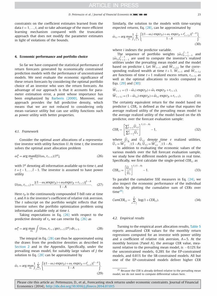
D. Pettenuzzo et al. / Journal of Financial Economics ] (]]]]) ]]]–]]] 23
constraints on the coefficient estimates learned from thedata t ¼ 1;…; t, and so take advantage of the more efficientlearning mechanism compared with the truncationapproach that does not modify the parameter estimatesin light of violations of the bounds.
4. Economic performance and portfolio choice
So far we have compared the statistical performance ofreturn forecasts generated by economically constrainedprediction models with the performance of unconstrainedmodels. We next evaluate the economic significance ofthese return forecasts by considering the optimal portfoliochoice of an investor who uses the return forecasts. Anadvantage of our approach is that it accounts for para-meter estimation error, a point whose importance hasbeen emphasized by Barberis (2000). Moreover, ourapproach provides the full predictive density, whichmeans that we are not reduced to considering onlymean–variance utility but can use utility functions suchas power utility with better properties.
20 Because the CER is already defined relative to the prevailing meanmodel, we do not need to compute differential values here.
4.1. Framework
Consider the optimal asset allocations of a representa-tive investor with utility function U. At time t, the investorsolves the optimal asset allocation problem
ωn
t ¼ arg maxωt
E½Uðωt ; rtþ1ÞjDt �; ð26Þ
with Dt denoting all information available up to time t, andt ¼ t�1;…; t�1. The investor is assumed to have powerutility
U ωt ; rtþ1ð Þ ¼ ½ð1�ωtÞexpðrftÞþωtexpðrftþrtþ1Þ�1�A
1�A: ð27Þ
Here rft is the continuously compounded T-bill rate at timet, and A is the investor's coefficient of relative risk aversion.The t subscript on the portfolio weight reflects that theinvestor solves the portfolio optimization problem usinginformation available only at time t.
Taking expectations in Eq. (26) with respect to thepredictive density of rt, we can rewrite Eq. (26) as
ωn
t ¼ arg maxωt
ZUðωt ; rtþ1Þpðrtþ1jDtÞ drtþ1: ð28Þ
The integral in Eq. (28) can thus be approximated usingthe draws from the predictive densities as described inSection 2 and in the Appendix. Specifically, under theprevailing mean model, for suitably large values of J thesolution to Eq. (28) can be approximated by
bωt ¼ arg maxωt
1J∑J
j ¼ 1
½ð1�ωtÞ expðrftÞþωt expðrftþrjtþ1Þ�1�A
1�A
( ):
ð29Þ
Please cite this article as: Pettenuzzo, D., et al., Forecasting stocEconomics (2014), http://dx.doi.org/10.1016/j.jfineco.2014.07.01
Similarly, the solution to the models with time-varyingexpected returns, Eq. (28), can be approximated by
bωt;i ¼ arg maxωt
1J∑J
j ¼ 1
½ð1�ωtÞ expðrftÞþωt expðrftþrjtþ1;iÞ�1�A
1�A
( );
ð30Þwhere i indexes the predictor variable.
The sequence of portfolio weights fbωtgt �1t ¼ t �1 and
fbωt;igt �1t ¼ t �1 are used to compute the investor's realized
utilities under the prevailing mean model and the modelbased on predictor i. Let cWtþ1 and cWtþ1;i be the corre-sponding realized wealth at time tþ1. cWtþ1 and cWtþ1;i
are functions of time tþ1 realized excess return, rtþ1, aswell as the optimal allocations to stocks computed inEqs. (29) and (30):cWtþ1 ¼ ð1� bωtÞ expðrftÞþ bωt expðrftþrtþ1Þ;cWtþ1;i ¼ ð1� bωt;iÞ expðrftÞþ bωt;i expðrftþrtþ1Þ: ð31Þ
The certainty equivalent return for the model based onpredictor i, CERi; is defined as the value that equates theaverage realized utility of the prevailing mean model tothe average realized utility of the model based on the ithpredictor, over the forecast evaluation sample:
CERi ¼∑t
τ ¼ tbU τ;i
∑tτ ¼ t
bU τ
24 351=ð1�AÞ
�1; ð32Þ
where bU τ and bU τ;i denote time τ realized utilities,bU τ ¼ cW 1�A
τ =ð1�AÞ, bU τ;i ¼ cW 1�A
τ;i =ð1�AÞ.In addition to evaluating the economic values of the
various models over the full forecast evaluation sample,we study how the different models perform in real time.Specifically, we first calculate the single-period CERt;i as
CERt;i ¼bUt;ibUt
" #1=ð1�AÞ
�1: ð33Þ
To parallel the cumulative SSE measures in Eq. (24), wealso inspect the economic performance of the individualmodels by plotting the cumulative sum of CERs overtime20:
CumCERt;i ¼ ∑t
τ ¼ tlogð1þCERt;iÞ: ð34Þ
4.2. Empirical results
Turning to the empirical asset allocation results, Table 5reports annualized CER values for the monthly returnregressions computed for an investor with power utilityand a coefficient of relative risk aversion, A¼5. At themonthly horizon (Panel A), the average CER value, mea-sured relative to the prevailing mean model, is �0.12% forthe unconstrained models, 0.28% for the EP-constrainedmodels, and 0.81% for the SR-constrained models. All butone of the EP-constrained models deliver higher CER
k returns under economic constraints. Journal of Financial5i
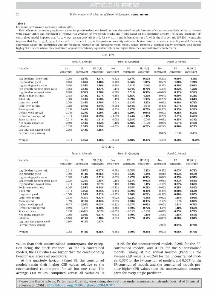
Table 6Economic performance measures: subsamples.
This table reports certainty equivalent values for portfolio decisions based on recursive out-of-sample forecasts of excess returns. Each period an investorwith power utility and coefficient of relative risk aversion of five selects stocks and T-bills based on his predictive density. The equity premium (EP)constrained model imposes that r̂ τþ1jt ¼
R ðμþβxτÞpðμ; βjDt Þ dμ dβ40; for τ¼ 1;…; t and information set Dt , while the Sharpe ratio (SR [0,1]) constraintimposes that 0r r̂ τþ1jt=σ̂ τþ1jtr1; for τ¼ 1;…; t, where σ̂ τþ1jt is the posterior volatility estimate obtained from a stochastic volatility model. Certaintyequivalent values are annualized and are measured relative to the prevailing mean model, which assumes a constant equity premium. Bold figureshighlight instances where the constrained annualized certainty equivalent values are higher than their unconstrained counterparts.
1947–1978
Panel A: Monthly Panel B: Quarterly Panel C: Annual
Variable No EP SR [0,1] No EP SR [0,1] No EP SR [0,1]constraint constraint constraint constraint constraint constraint constraint constraint constraint
Log dividend–price ratio 0.06% 0.57% 1.41% 0.22% 0.67% 0.82% 0.22% 0.69% 1.11%Log dividend yield 0.16% 0.68% 1.46% 0.30% 0.66% 1.05% 0.69% 1.00% 1.21%Log earning–price ratio 0.19% 0.54% 1.16% 0.30% 0.61% 0.16% 0.33% 0.59% 0.64%Log smooth earning–price ratio �0.36% 0.52% 1.47% �0.14% 0.64% 0.70% 0.13% 0.82% 1.22%Log dividend–payout ratio 0.18% 0.51% 1.28% 0.20% 0.51% 0.36% �0.02% 0.52% 0.58%Book-to-market ratio �0.48% 0.48% 1.01% �0.35% 0.58% 0.10% 0.04% 0.59% 0.23%T-Bill rate 0.30% 0.43% 1.88% 0.19% 0.39% 1.38% �0.29% 0.52% 0.64%Long-term yield 0.04% 0.44% 1.79% 0.01% 0.43% 1.17% 0.06% 0.49% 0.71%Long-term return �0.38% 0.47% 1.94% �0.08% 0.44% �0.14% 0.40% 0.71% 0.59%Term spread 0.33% 0.46% 1.50% 0.25% 0.47% 0.70% �0.30% 0.55% 0.33%Default yield spread �0.04% 0.27% 1.09% �0.15% 0.30% 0.04% �0.02% 0.36% 0.27%Default return spread �0.31% 0.49% 0.89% �1.09% 0.24% �0.11% 0.20% 0.51% 0.40%Stock variance 0.01% 0.15% 1.11% 0.05% 0.28% 0.04% 0.03% 0.35% 0.34%Net equity expansion 0.19% 0.43% 1.22% 0.10% 0.48% �0.02% 0.06% 0.51% 0.45%Inflation �0.03% 0.38% 1.29% �0.03% 0.44% 0.27% �0.24% 0.46% 0.27%Log total net payout yield 0.26% 0.48% 1.18%Percent equity issuing 0.86% 0.53% 0.45%
Average 0.01% 0.46% 1.36% �0.02% 0.48% 0.43% 0.13% 0.58% 0.59%
1979-2010
Panel A: Monthly Panel B: Quarterly Panel C: Annual
Variable No EP SR [0,1] No EP SR [0,1] No EP SR [0,1]constraint constraint constraint constraint constraint constraint constraint constraint constraint
Log dividend–price ratio �0.61% 0.07% 0.07% �0.58% 0.08% 0.17% �0.47% 0.07% 0.72%Log dividend yield �0.69% 0.14% 0.06% �0.45% 0.12% 0.18% �0.81% �0.02% 0.57%Log earning–price ratio 0.08% 0.44% 0.51% 0.05% 0.47% 0.52% 0.02% 0.35% 0.97%Log smooth earning–price ratio �0.22% 0.25% 0.15% �0.19% 0.23% 0.02% �0.08% 0.32% 0.83%Log dividend–payout ratio 0.21% 0.23% 0.12% 0.10% 0.19% 0.11% �0.16% 0.07% 0.68%Book-to-market ratio �1.04% 0.08% 0.24% �0.73% 0.18% 0.28% �0.60% 0.28% 0.86%T-Bill rate �0.61% 0.06% 0.25% �0.45% 0.09% 0.31% �0.46% 0.00% 0.63%Long-term yield �0.56% 0.06% 0.21% �0.47% 0.10% 0.22% �0.58% 0.00% 0.80%Long-term return 0.33% 0.23% 0.87% 0.02% 0.22% 0.16% 0.02% 0.15% 0.92%Term spread 0.09% 0.11% 0.42% 0.05% 0.10% 0.33% 0.19% 0.07% 0.82%Default yield spread �0.17% �0.06% 0.03% �0.22% �0.07% �0.03% �0.05% 0.11% 0.74%Default return spread 0.19% 0.13% 0.40% �0.38% �0.19% 0.72% �1.15% �0.10% 0.67%Stock variance 0.33% �0.44% 0.12% �0.05% �0.28% �0.43% �0.08% 0.05% 0.79%Net equity expansion �0.29% 0.06% 0.31% �0.63% 0.10% 0.11% �3.55% �0.15% 0.56%Inflation �0.16% 0.15% 0.16% 0.07% 0.17% 0.51% �0.08% 0.06% 0.84%Log total net payout yield �0.86% 0.11% 0.17%Percent equity issuing �2.02% �0.04% 0.72%
Average �0.25% 0.10% 0.26% �0.26% 0.10% 0.21% �0.62% 0.08% 0.76%
D. Pettenuzzo et al. / Journal of Financial Economics ] (]]]]) ]]]–]]]24
values than their unconstrained counterparts, the excep-tion being the stock variance. For the SR-constrainedmodels, the CER values are higher than the correspondingbenchmarks across all predictors.
At the quarterly horizon (Panel B), the constrainedmodels retain their higher CER values relative to theunconstrained counterparts for all but one case. Theaverage CER values, computed across all variables, is
Please cite this article as: Pettenuzzo, D., et al., Forecasting stocEconomics (2014), http://dx.doi.org/10.1016/j.jfineco.2014.07.01
�0.14% for the unconstrained models, 0.29% for the EP-constrained models, and 0.32% for the SR-constrainedmodels. Finally, at the annual horizon (Panel C), theaverage CER value is �0.24% for the unconstrained mod-els, 0.33% for the EP-constrained models, and 0.67% for theSR-constrained models and the constrained models pro-duce higher CER values than the unconstrained counter-parts for every single predictor.
k returns under economic constraints. Journal of Financial5i

Per
cent
wei
ght t
o st
ocks
1940 1945 1950 1955 1960 1965 1970 1975 1980 1985 1990 1995 2000 2005
0
20
40
60
80
100
120
Con
tinuo
usly
com
poun
ded
C
ER
s (p
erce
nt)
Log dividend−price ratio − recursive CRRA cumulative CERs
Log dividend−price ratio − recursive CRRA weights to stocks
1940 1945 1950 1955 1960 1965 1970 1975 1980 1985 1990 1995 2000 2005
−50
0
50
100
150
Fig. 14. Portfolio allocation and economic value of forecasts. This figure plots the percentage allocation to stocks and the resulting cumulative certaintyequivalent returns (CERs) measured relative to the prevailing mean model. Each month we compute the optimal allocation to stocks and T-bills based onthe predictive density of excess returns. The investor is assumed to have power utility with a coefficient of relative risk aversion of five and the weight onstocks is constrained to lie in the interval ½0;0:99�. The top graph shows the recursively computed optimal weight on stocks, and the bottom graph showsthe cumulative certainty equivalent return measured relative to the prevailing mean model. The equity premium constrained model imposes the constraintthat r̂ τþ1jt ¼
R ðμþβxτÞpðμ; βjDt Þ dμ dβ40; for τ¼ 1;…; t and information set Dt , and the Sharpe ratio constrained models impose that 0r r̂ τþ1jt=σ̂ τþ1jtr1;for τ¼ 1;…; t, where σ̂ τþ1jt is the posterior volatility estimate obtained from either a constant volatility model (CV) or a stochastic volatility model (SV). Thepredictor used is the log dividend–price ratio. CRRA: constant relative risk aversion.
D. Pettenuzzo et al. / Journal of Financial Economics ] (]]]]) ]]]–]]] 25
Comparing the results under the truncation approachof Campbell and Thompson (2008) with those under theEP constraint, Table 5 shows that, with one exception(stock variance, monthly horizon), the EP approach gen-erates higher CER values for all predictors at all horizons.The average improvement in CER values is 0.35% (from�0.07% to 0.28%), 0.37% (from �0.08% to 0.29%), and0.50% (from �0.17% to 0.33%) at the monthly, quarterly,and annual horizon, respectively. Given the better perfor-mance under the EP constraint than under the truncationapproach, we do not report further results from the latter.
In Table 6, we show that the observed improvements ineconomic utility carry over to our two subsamples. Thereagain, the constrained models do better than the uncon-strained ones for the vast majority of cases. Interestingly,no evidence suggests that the economic benefits fromusing economically constrained forecasts deterioratesover time. For example, over the subsample 1979–2010the mean CER value for the annual model is �0.62% forthe unconstrained model and 0.08% and 0.76% for theEP- and SR-constrained models, a bigger differential thanin the earlier subsample 1947–1978.
Using the log dividend–price ratio as a predictor, Fig. 14plots the sequence of stock portfolio weights along withthe cumulative (continuously compounded) CER estimatescomputed according to Eq. (34). The portfolio weights varyconsiderably over time under the unconstrained and SR-constrained model that allows for stochastic volatility, butthey are much smoother under the EP constraint and theconstant-volatility SR-constrained model. Moreover, the
Please cite this article as: Pettenuzzo, D., et al., Forecasting stocEconomics (2014), http://dx.doi.org/10.1016/j.jfineco.2014.07.01
cumulative CER values of the constrained models consis-tently lie above the CER estimates of the unconstrainedmodel. At the end of the sample, the cumulative CER valueof the unconstrained model is around �30%, and itexceeds 20% and 80% for the EP- and SR- (stochasticvolatility) constrained models, respectively. These num-bers capture the cumulative risk-adjusted economic valueof the economically constrained forecasts relative to theprevailing mean forecasts.
We conclude that economically large benefits arederived from imposing economic constraints on the equitypremium prediction models. The benefits appear to bepresent at monthly, quarterly, and annual horizons and arelargest for the SR constraint that allows for time-varyingvolatility. Moreover, the benefits do not appear to bedeteriorating over time.
5. Extensions and robustness analysis
This section extends our analysis to incorporate multi-variate information. Moreover, we present a range ofsensitivity analyses that shed light on the robustness ofour findings.
5.1. Multivariate results
So far, we follow much of the finance literature onreturn predictability and focus on univariate predictionmodels. We next extend the analysis to a multivariatesetting. With N predictor variables available, there are N
k returns under economic constraints. Journal of Financial5i

Table 7Out-of-sample forecast and economic performance: Multivariate methods.
Panel A reports the out-of-sample R2 of unconstrained and constrained multivariate prediction models for the excess return, rtþ1, measured relative tothe prevailing mean model:
R2OoS ¼ 1�
∑t �1τ ¼ t �1ðrtþ1� r̂ tþ1jt Þ2
∑t �1τ ¼ t �1ðrtþ1�r tþ1jt Þ2
;
where r̂ tþ1jt is the posterior mean of the predictive return distribution based on either an equal-weighted forecast combination or a diffusion indexapproach. The equity premium (EP) constrained model imposes that r̂ τþ1jt40; for τ¼ 1;…; t and information set Dt , and the Sharpe ratio (SR [0,1])constraint imposes that 0r r̂ τþ1jt=σ̂ τþ1jtr1; for τ¼ 1;…; t, where σ̂ τþ1jt is the posterior volatility estimate obtained from a stochastic volatility model.Panel B reports certainty equivalent values for portfolio decisions based on recursive out-of-sample forecasts of excess returns. Each period an investorwith power utility and coefficient of relative risk aversion of five selects stocks and T-bills based on his predictive density. Certainty equivalent values areannualized and are measured relative to the prevailing mean model, which assumes a constant equity premium. Bold figures highlight instances in whichthe constrained ROoS
2(Panel A) or annualized certainty equivalent returns (Panel B) are higher than their unconstrained counterparts. nsignificance at 10%
level; nnsignificance at 5% level; nnnsignificance at 1% level.
Monthly Quarterly Annual
Method No EP SR [0,1] No EP SR [0,1] No EP SR [0,1]constraint constraint constraint constraint constraint constraint constraint constraint constraint
Panel A: Forecast performance (out of sample R2)
Full sample
Equal-weighted combination 0.62%nnn 0.25%n 0.31%n 1.19%nn 0.77%n 1.32%nnn 4.48%nn 4.13%nn 4.45%nnn
Diffusion index 0.23%nn 0.74%nnn 0.76%nnn 0.42%nn 3.02%nnn 2.95%nnn �1.53% 7.57%nnn 6.33%nnn
1947-1978
Equal-weighted combination 1.09%nnn 0.53%n 0.65%n 2.57%nn 1.59%n 2.38%nnn 9.26%nnn 8.06%nn 7.99%nnn
Diffusion index 1.62%nnn 1.46%nnn 1.53%nnn 3.09%nn 4.99%nnn 4.93%nnn 1.71% 13.68%nnn 11.44%nnn
1979–2010
Equal-weighted combination 0.26% 0.06% 0.09% �0.02% 0.07% 0.40% �0.50% 0.04% 0.76%Diffusion index �0.83% 0.22% 0.19% �1.89% 1.32%n 1.24%n �4.89% 1.21% 1.00%
Panel B: Economic performance (certainty equivalent return)
Full sample
Equal-weighted combination 0.14% 0.27% 0.86% 0.02% 0.33% 0.41% 0.07% 0.37% 0.69%Diffusion index �0.07% 0.44% 1.02% �0.04% 0.53% 0.95% �0.25% 0.46% 1.02%
D. Pettenuzzo et al. / Journal of Financial Economics ] (]]]]) ]]]–]]]26
different predictive densities. Using i to index the pre-dictors as above, we denote these predictive densities bypðrtþ1jDt ;MiÞ, i¼ 1;…;N, where Mi refers to model i.Instead of conditioning only on a single predictor, inves-tors could take advantage of the information contained inall of the N predictors. We consider two different ways tocombine the information contained in N differentpredictors.
The first approach relies on forecast combination meth-ods. Specifically, we construct a combined predictive densityas an equal-weighted average of the N predictive densities
pðrtþ1jDtÞ ¼ ∑N
i ¼ 1wi;t � pðrtþ1jDt ;MiÞ; ð35Þ
where wi;t ¼ 1=N for all i and t ¼ t�1;…; t�1. We computethe equal-weighted predictive density in Eq. (35) across allpredictor variables applying this approach separately to theunconstrained, EP-, and SR-constrained models. For pointforecasts, this approach was previously adopted by Rapach,Strauss, and Zhou (2010).
Our second approach relies on diffusion indexes. Asshown by Stock and Watson (2006), diffusion indexes
Please cite this article as: Pettenuzzo, D., et al., Forecasting stocEconomics (2014), http://dx.doi.org/10.1016/j.jfineco.2014.07.01
provide a convenient framework for extracting the keycommon drivers from a large number of potential pre-dictors. Ludvigson and Ng (2007) and Neely, Rapach, Tu,and Zhou (2012) show that diffusion indexes can be usedto improve equity premium forecasting.
The diffusion index approach assumes a common factorstructure for the N potential predictors,
xiτ ¼ λ0if τþei;τ ; τ¼ 1;…; t�1 ð36Þ
where i indexes the predictor, λ is a ðq� 1Þ vector of factorloadings (q5N), f τ is a ðq� 1Þ vector of latent factorscontaining the common components extracted from the Npredictors, and ei;τ is a zero-mean disturbance term.Following Rapach, Strauss, and Zhou (2010), we restrictour analysis to considering a single factor. The results donot appear to improve if we include two or more factors inthe model.
We estimate the common factors using principal com-ponents as predictors for stock returns
rτþ1 ¼ μDIþβDIf τþετþ1; τ¼ 1;…; t�1; ð37Þ
k returns under economic constraints. Journal of Financial5i
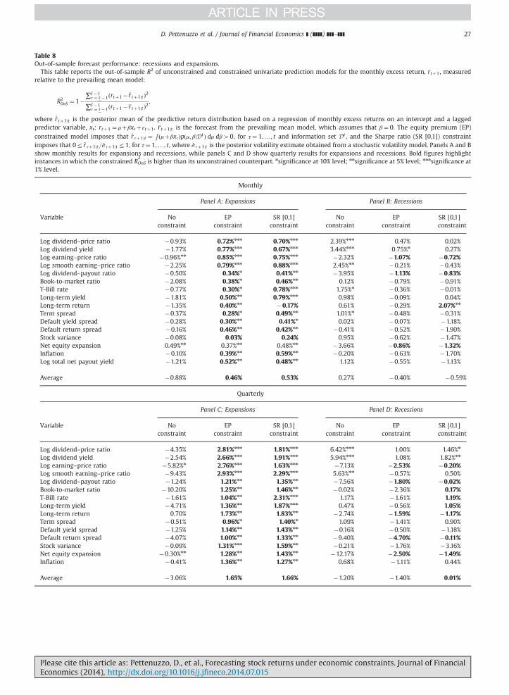
Table 8Out-of-sample forecast performance: recessions and expansions.
This table reports the out-of-sample R2 of unconstrained and constrained univariate prediction models for the monthly excess return, rtþ1, measuredrelative to the prevailing mean model:
R2OoS ¼ 1�
∑t �1τ ¼ t �1ðrtþ1� r̂ tþ1jt Þ2
∑t �1τ ¼ t �1ðrtþ1�r tþ1jt Þ2
;
where r̂ tþ1jt is the posterior mean of the predictive return distribution based on a regression of monthly excess returns on an intercept and a laggedpredictor variable, xt: rtþ1 ¼ μþβxtþεtþ1. r tþ1jt is the forecast from the prevailing mean model, which assumes that β¼ 0. The equity premium (EP)constrained model imposes that r̂ τþ1jt ¼
R ðμþβxτÞpðμ; βjDt Þ dμ dβ40; for τ¼ 1;…; t and information set Dt , and the Sharpe ratio (SR [0,1]) constraintimposes that 0r r̂ τþ1jt=σ̂ τþ1jtr1; for τ¼ 1;…; t, where σ̂ τþ1jt is the posterior volatility estimate obtained from a stochastic volatility model. Panels A and Bshow monthly results for expansions and recessions, while panels C and D show quarterly results for expansions and recessions. Bold figures highlightinstances in which the constrained ROoS
2is higher than its unconstrained counterpart. nsignificance at 10% level; nnsignificance at 5% level; nnnsignificance at
1% level.
Monthly
Panel A: Expansions Panel B: Recessions
Variable No EP SR [0,1] No EP SR [0,1]constraint constraint constraint constraint constraint constraint
Log dividend–price ratio �0.93% 0.72%nnn 0.70%nnn 2.39%nnn 0.47% 0.02%Log dividend yield �1.77% 0.77%nnn 0.67%nnn 3.44%nnn 0.75%n 0.27%Log earning–price ratio �0.96%nn 0.85%nnn 0.75%nnn �2.32% �1.07% �0.72%Log smooth earning–price ratio �2.25% 0.79%nnn 0.88%nnn 2.45%nn �0.21% �0.43%Log dividend–payout ratio �0.50% 0.34%n 0.41%nn �3.95% �1.13% �0.83%Book-to-market ratio �2.08% 0.38%n 0.46%nn 0.12% �0.79% �0.91%T-Bill rate �0.77% 0.30%n 0.78%nnn 1.75%n �0.36% �0.01%Long-term yield �1.81% 0.50%nn 0.79%nnn 0.98% �0.09% 0.04%Long-term return �1.35% 0.40%nn �0.17% 0.61% �0.29% 2.07%nn
Term spread �0.37% 0.28%n 0.49%nn 1.01%n �0.48% �0.31%Default yield spread �0.28% 0.30%nn 0.41%n 0.02% �0.07% �1.18%Default return spread �0.16% 0.46%nn 0.42%nn �0.41% �0.52% �1.90%Stock variance �0.08% 0.03% 0.24% 0.95% �0.62% �1.47%Net equity expansion 0.49%nn 0.37%nn 0.48%nn �3.66% �0.86% �1.32%Inflation �0.10% 0.39%nn 0.59%nn �0.20% �0.63% �1.70%Log total net payout yield �1.21% 0.52%nn 0.48%nn 1.12% �0.55% �1.13%
Average �0.88% 0.46% 0.53% 0.27% �0.40% �0.59%
Quarterly
Panel C: Expansions Panel D: Recessions
Variable No EP SR [0,1] No EP SR [0,1]constraint constraint constraint constraint constraint constraint
Log dividend–price ratio �4.35% 2.81%nnn 1.81%nnn 6.42%nnn 1.00% 1.46%n
Log dividend yield �2.54% 2.66%nnn 1.91%nnn 5.94%nnn 1.08% 1.82%nn
Log earning–price ratio �5.82%n 2.76%nnn 1.63%nnn �7.13% �2.53% �0.20%Log smooth earning–price ratio �9.43% 2.93%nnn 2.29%nnn 5.63%nn �0.57% 0.50%Log dividend–payout ratio �1.24% 1.21%nn 1.35%nn �7.56% �1.80% �0.02%Book-to-market ratio �10.20% 1.25%nn 1.46%nn �0.02% �2.36% 0.17%T-Bill rate �1.61% 1.04%nn 2.31%nnn 1.17% �1.61% 1.19%Long-term yield �4.71% 1.36%nn 1.87%nnn 0.47% �0.56% 1.05%Long-term return 0.70% 1.73%nn 1.83%nn �2.74% �1.59% �1.17%Term spread �0.51% 0.96%n 1.40%n 1.09% �1.41% 0.90%Default yield spread �1.25% 1.14%nn 1.43%nn �0.16% �0.50% �1.18%Default return spread �4.07% 1.00%nn 1.33%nn �9.40% �4.70% �0.11%Stock variance �0.09% 1.31%nnn 1.59%nn �0.21% �1.76% �3.16%Net equity expansion �0.30%nn 1.28%nn 1.43%nn �12.17% �2.50% �1.49%Inflation �0.41% 1.36%nn 1.27%nn 0.68% �1.11% 0.44%
Average �3.06% 1.65% 1.66% �1.20% �1.40% 0.01%
Please cite this article as: Pettenuzzo, D., et al., Forecasting stock returns under economic constraints. Journal of FinancialEconomics (2014), http://dx.doi.org/10.1016/j.jfineco.2014.07.015i
D. Pettenuzzo et al. / Journal of Financial Economics ] (]]]]) ]]]–]]] 27

Table 9Sensitivity analysis for the upper bound on the Sharpe ratio.
Panel A reports the out-of-sample R2 of unconstrained and constrained univariate prediction models for monthly excess returns, rtþ1, measured relativeto the prevailing mean model:
R2OoS ¼ 1�
∑t �1τ ¼ t �1ðrtþ1� r̂ tþ1jt Þ2
∑t �1τ ¼ t �1ðrtþ1�r tþ1jt Þ2
;
where r̂ tþ1jt is the mean of the predictive return distribution based on a regression of excess returns on an intercept and a lagged predictor variable, xt:rtþ1 ¼ μþβxtþεtþ1. r tþ1jt is the forecast from the prevailing mean model, which assumes that β¼ 0. The equity premium (EP) constrained model imposesthat r̂ τþ1jt ¼
R ðμþβxτÞpðμ; βjDt Þ dμ dβ40; for τ¼ 1;…; t and information set Dt , and the Sharpe ratio (SR) constraint imposes that r̂ tþ1jt=σ̂ tþ1jt is boundedbetween 0 and the specified upper bound, where σ̂ τþ1jt is the posterior volatility estimate obtained from a stochastic volatility model and t ¼ 1;…; T�1.Panel B reports certainty equivalent values for portfolio decisions based on recursive out-of-sample forecasts of excess returns. Each period an investorwith power utility and coefficient of relative risk aversion of five selects stocks and T-bills based on his predictive density. Certainty equivalent values areannualized and are measured relative to the prevailing mean model, which assumes a constant equity premium. Bold figures highlight instances in whichthe constrained ROoS
2(Panel A) or annualized certainty equivalent returns (Panel B) are higher than their unconstrained counterparts. nsignificance at 10%
level; nnsignificance at 5% level; nnnsignificance at 1% level.
Panel A: Forecast performance (out of sample R2)
Variable No EP SR [0,0.5] SR [0,0.75] SR [0,1] SR [0,1.25] SR [0,1.5]constraint constraint constraint constraint constraint constraint constraint
Log dividend–price ratio 0.10%n 0.64%nnn 0.17% 0.50%nnn 0.49%nn 0.54%nn 0.48%nn
T-Bill rate 0.01%n 0.10% 0.33%nn 0.58%nnn 0.54%nn 0.60%nn 0.60%nn
Default yield spread �0.19% 0.18% 0.14% 0.20% �0.08% �0.26% �0.31%
Panel B: Economic performance (certainty equivalent return)
Variable No EP SR [0,0.5] SR [0,0.75] SR [0,1] SR [0,1.25] SR [0,1.5]constraint constraint constraint constraint constraint constraint constraint
Log dividend–price ratio �0.28% 0.32% 0.20% 0.57% 0.74% 0.93% 0.96%T-Bill rate �0.15% 0.25% 0.38% 0.83% 1.06% 1.33% 1.48%Default yield spread �0.11% 0.10% 0.19% 0.49% 0.56% 0.68% 0.74%
D. Pettenuzzo et al. / Journal of Financial Economics ] (]]]]) ]]]–]]]28
where βDI is a ðq� 1Þ vector of slope coefficients andετþ1 �Nð0;σ2
ε;DIÞ. As for the univariate models in Section 2,we specify an independent normal-gamma prior for theparameters in Eq. (37), and use a Gibbs sampler forestimation. Next, draws from the corresponding predictivedensity are obtained as
pðrtþ1jDtÞ ¼ZμDI ;βDI ;σ � 2
ε;DI
pðrtþ1jμDI ;βDI ;σ�2ε;DI ;DtÞ
�pðμDI ;βDI ;σ�2ε;DIjDtÞ dμDI dβDI dσ
�2ε;DI ð38Þ
where pðμDI ;βDI ;σ�2ε;DIjDtÞ is the joint posterior density of
all parameters in Eq. (37). We estimate the diffusion indexmodel in Eq. (37) and derive the predictive density in Eq.(38) for the unconstrained, EP-constrained, and SR-constrained models.
5.1.1. Empirical findingsTable 7 presents empirical results for the equal-
weighted combination as well as for the diffusion index.First consider the statistical measures of forecast perfor-mance. In all cases these improve when compared withthe average forecast performance computed across theindividual models. At all three horizons, the equal-weighted combination yields the largest improvement inROoS2
performance for the unconstrained models. For exam-ple, at the monthly horizon the equal-weighted combina-tion of unconstrained forecasts generates a ROoS
2of 0.62%
versus �0.53% as the average value of the individualmodels. We also see improvements for the constrained
Please cite this article as: Pettenuzzo, D., et al., Forecasting stocEconomics (2014), http://dx.doi.org/10.1016/j.jfineco.2014.07.01
models, but these tend to be smaller. Which equal-weighted combination is best depends on the frequency.At the monthly horizon, combining unconstrained fore-casts seem to work best. At the quarterly horizon, combin-ing the SR-constrained forecasts produces the bestperformance. And at the annual horizon the threeapproaches perform comparably.
The performance improves even more in the case of thediffusion index that works particularly well under theeconomic constraints. In fact, the EP-constrained forecastsdeliver higher ROoS
2values than the equal-weighted uncon-
strained forecasts at all three horizons and across bothsubsamples. The SR-constrained forecasts based on thediffusion index also perform very well.
Turning to the economic performance measures, again,these generally lead to higher CER values when comparedagainst the average values produced by the individual uni-variate models. While the benefit from using equal-weightedforecasts remains largest for the unconstrained forecasts, theresulting CER values are always smaller than those produced bythe corresponding equal-weighted constrained forecasts withdifferences ranging from 0.13% to 0.31% for the EP-constrainedforecasts and from 0.39% to 0.72% for the SR-constrainedforecasts. Moreover, the best results from using the diffusionindex is obtained for the constrained forecasts with differencesranging from 0.51% to 0.71% for the EP-constrained forecastsand from 0.99% to 1.27% for the SR-constrained forecasts. Infact, the diffusion index approach works better than the equal-weighted combination for the EP-constrained and the SR-constrained cases at all horizons.
k returns under economic constraints. Journal of Financial5i

D. Pettenuzzo et al. / Journal of Financial Economics ] (]]]]) ]]]–]]] 29
5.2. Performance in recessions and expansions
Table 8 shows results separately for recession andexpansion periods as defined by the National Bureau ofEconomic Research (NBER) indicator and applied to themonthly and quarterly data. This type of analysis has beenproposed by authors such as Rapach, Strauss, and Zhou(2010) and Henkel, Martin, and Nardari (2011). Consistentwith the findings in these studies, the unconstrained returnprediction models perform better versus the prevailingmean during recessions than during expansions. Interest-ingly, the converse holds for the constrained monthlyforecasts that far outperform the unconstrained forecastsduring expansions but perform worse during recessions.
While seemingly surprising, this finding can beexplained by the fact that the state variable being sortedon (recessions) is correlated with returns. Returns tend tobe negative during recessions and positive during expan-sions and so models that impose non-negative predictionswill almost by construction do relatively better duringexpansions and worse during recessions.
Despite this effect, at the quarterly horizon the EP-constrained forecasts do almost as well as the uncon-strained forecasts during recessions (and much betterduring expansions), and the SR-constrained forecasts dosubstantially better than the unconstrained forecasts bothduring expansions and recessions.
5.3. Upper bound on Sharpe ratio
In practice it can be difficult to determine the upperbound on reasonable Sharpe ratios. Ross (1976) introducesasset pricing constraints by assuming that portfolios cannothave Sharpe ratios greater than twice the Sharpe ratio ofthe market portfolio, which would be roughly in line with(though a bit below) the upper bound SRu ¼ 1 that we focuson here. Cochrane and Saa-Requejo (2000) are less specificbut point out that there is a “long tradition in finance thatregards high Sharpe ratios as ‘good deals’ that are unlikelyto survive, since investors would quickly grab them up.”
One way to approach this issue is to view the upperbound as another parameter about which there is uncer-tainty and then conduct a sensitivity analysis. To this end,Table 9 shows results for the three predictors of particularfocus (the dividend–price ratio, the T-bill rate, and thedefault yield spread) for a wide range of values for theupper bound on the Sharpe ratio {0.5, 0.75, 1, 1.25, 1.5}. Thetable shows that the ROoS
2value is even higher than in the
baseline scenario with SRu ¼ 1 when the upper bound is setto 0.75, instead of one, although for two of the predictors(the dividend–price ratio and the T-bill rate), a larger valueof the upper bound (SRu ¼ 1:25) gives the best results. At thequarterly and annual horizons (not shown), slight improve-ments are observed (relative to the benchmark SRu ¼ 1) byeither increasing or decreasing SRu by 0.25, but the conclu-sions about the performance of the return forecasts underthe SR constraint again appear robust. Another perspectiveon this issue is that, given one's beliefs on what couldconstitute a reasonable upper bound on the Sharpe ratio, wecan use our proposed methodology to impose the resultingconstraint on the predictive regression.
Please cite this article as: Pettenuzzo, D., et al., Forecasting stocEconomics (2014), http://dx.doi.org/10.1016/j.jfineco.2014.07.01
5.4. Sensitivity to risk aversion
Our main analysis of the economic value of equitypremium forecasts in Section 4 assumes a coefficient ofrelative risk aversion of A¼5. To explore the sensitivity ofour results to this value, we also consider lower (A¼2) andhigher (A¼10) values of this parameter. Results are shownin Table 10.
First consider the case with A¼2, i.e., lower risk aversioncompared with the baseline case, A¼5. At the monthlyhorizon, the average CER performance of the unconstrainedperformance models is reduced from �0.12% to �0.27%.Conversely, the average CER value of the EP-constrainedmodels increases from 0.28% to 0.68% and the SR constrainedmodels’ average performance is essentially unchanged at0.79%. At the quarterly horizon, the mean CER value of theunconstrained forecasts remains unchanged. The mean CERvalues under the EP and SR constraints increase from around0.3% to 0.8% and 1.0%, respectively. Similarly, the constrainedmodels’ mean CER values increase to 0.83% and 1.03%,respectively (previously 0.33% and 0.67%) at the annualhorizon, and the unconstrained model's mean CER value,at �0.07%, remains negative (previously �0.24%). Loweringthe coefficient of risk aversion from A¼5 to A¼2 thus hasthe effect of boosting the economic performance of theconstrained models whose mean CER value exceeds that ofthe unconstrained model by more than 0.90% (EP constraint)and 1.06% (SR constraint).
Increasing the risk aversion from A¼5 to A¼10 reducesthe spread in the performance of the different models, asan investor with such a high level of risk aversion refrainsfrom taking large positions in equity even in the presenceof strong evidence of return predictability. At this higherlevel of risk aversion, the constrained models continueto outperform the unconstrained ones, although thedifference in average CER values is reduced to between0.2% and 0.35% for the EP-constrained models and tobetween 0.3% and 0.5% for the SR-constrained models.
5.5. Sensitivity to priors
We also test the robustness of our results to alternativeprior assumptions and perform a sensitivity analysis inwhich we experiment with different values for some of thekey prior hyperparameters. Given the similarities in theresults obtained under the models based on the EP and SRconstraints, as well as the more computationally demand-ing estimation algorithm required by models imposing theSR constraint, we focus our attention on the effectivenessof the equity premium constraint as the priors change andexplore the effect of altering the hyperparameter ψ and v0in Eqs. (10) and (13). As discussed in Section 2.2, thehyperparameter ψ plays the role of a scaling factorcontrolling the tightness of the priors for μ and β, andour benchmark models set ψ ¼ 2:5. As sensitivities, weexperiment with ψ ¼ 1:25 and ψ ¼ 5, which imply moreconcentrated prior distributions (in the case of ψ ¼ 1:25)or more dispersed prior distributions (in the case of ψ ¼ 5)for μ and β. Similarly, the prior parameter v0 controls thetightness of the prior for σ�2
ε , and our benchmark models
k returns under economic constraints. Journal of Financial5i

Table 10Effect of risk aversion on economic performance measures.
This table reports certainty equivalent values for portfolio decisions based on recursive out-of-sample forecasts of excess returns. Each period an investorwith power utility and coefficient of relative risk aversion of two (top panels) or ten (bottom panels) selects stocks and T-bills based on his predictivedensity. The equity premium (EP) constrained model imposes that r̂ τþ1jt ¼
R ðμþβxτÞpðμ; βjDt Þ dμ dβ40; for τ¼ 1;…; t and information set Dt , and theSharpe ratio (SR [0,1]) constraint imposes that 0r r̂ τþ1jt=σ̂ τþ1jtr1; for τ¼ 1;…; t, where σ̂ τþ1jt is the posterior volatility estimate obtained from astochastic volatility model. Certainty equivalent values are annualized and are measured relative to the prevailing mean model, which assumes a constantequity premium. Bold figures highlight instances in which the constrained annualized certainty equivalent values are higher than their unconstrainedcounterparts.
A¼2
Panel A: Monthly Panel B: Quarterly Panel C: Annual
Variables No EP SR [0,1] No EP SR [0,1] No EP SR [0,1]constraint constraint constraint constraint constraint constraint constraint constraint constraint
Log dividend–price ratio �0.89% 0.68% 0.78% �0.47% 0.90% 1.02% �0.20% 0.83% 1.09%Log dividend yield �1.06% 0.66% 0.77% �0.22% 0.92% 1.00% �0.51% 0.90% 1.09%Log earning–price ratio 0.15% 1.04% 0.75% 0.32% 1.41% 0.96% 0.36% 1.09% 1.06%Log smooth earning–price ratio �1.11% 0.72% 0.78% �0.85% 0.96% 1.14% �0.33% 1.04% 1.08%Log dividend–payout ratio 0.70% 0.83% 0.64% 0.79% 0.86% 0.93% 0.15% 0.76% 1.00%Book-to-market ratio �1.36% 0.73% 0.73% �1.05% 1.13% 1.06% �0.64% 1.13% 1.24%T-Bill rate �0.29% 0.64% 0.89% �0.24% 0.59% 1.03% �0.92% 0.71% 1.01%Long-term yield �0.69% 0.61% 0.72% �0.54% 0.63% 0.94% �0.71% 0.65% 1.02%Long-term return �0.12% 0.77% 1.31% �0.11% 0.82% 0.67% 0.38% 0.87% 1.07%Term spread 0.67% 0.76% 0.82% 0.85% 0.71% 1.02% �0.07% 0.84% 1.03%Default yield spread �0.17% 0.33% 0.83% �0.37% 0.37% 1.08% �0.11% 0.53% 1.02%Default return spread 0.01% 0.76% 0.83% �1.17% 0.68% 1.01% 0.10% 0.80% 1.02%Stock variance 0.34% 0.26% 0.74% 0.00% 0.36% 1.13% �0.09% 0.48% 1.00%Net equity expansion 0.45% 0.72% 0.77% 0.71% 0.91% 0.99% 0.52% 0.96% 0.93%Inflation �0.12% 0.69% 0.59% 0.03% 0.73% 0.97% �0.01% 0.83% 0.98%Log total net payout yield �0.83% 0.73% 0.69%Percent equity issuing 1.02% 0.85% 0.91%
Average �0.27% 0.68% 0.79% �0.15% 0.80% 1.00% �0.07% 0.83% 1.03%
A¼10
Panel A: Monthly Panel B: Quarterly Panel C: Annual
Variable No EP SR [0,1] No EP SR [0,1] No EP SR [0,1]constraint constraint constraint constraint constraint constraint constraint constraint constraint
Log dividend–price ratio �0.13% 0.18% 0.39% �0.10% 0.19% 0.27% �0.09% 0.19% 0.49%Log dividend yield �0.13% 0.20% 0.41% �0.06% 0.19% 0.34% �0.04% 0.27% 0.47%Log earning–price ratio 0.08% 0.27% 0.44% 0.09% 0.26% 0.19% 0.04% 0.24% 0.44%Log smooth earning–price ratio �0.15% 0.20% 0.43% �0.10% 0.23% 0.21% �0.05% 0.29% 0.55%Log dividend–payout ratio 0.12% 0.19% 0.36% 0.09% 0.18% 0.16% �0.03% 0.17% 0.32%Book-to-market ratio �0.36% 0.16% 0.33% �0.25% 0.20% 0.12% �0.16% 0.24% 0.29%T-Bill rate �0.08% 0.13% 0.55% �0.08% 0.12% 0.44% �0.20% 0.15% 0.35%Long-term yield �0.13% 0.13% 0.52% �0.14% 0.13% 0.36% �0.13% 0.14% 0.40%Long-term return 0.00% 0.19% 0.74% �0.03% 0.17% �0.02% 0.08% 0.24% 0.37%Term spread 0.12% 0.16% 0.49% 0.06% 0.15% 0.29% �0.07% 0.18% 0.32%Default yield spread �0.04% 0.06% 0.29% �0.10% 0.05% 0.03% �0.02% 0.13% 0.27%Default return spread �0.07% 0.16% 0.28% �0.38% 0.02% 0.21% �0.25% 0.12% 0.28%Stock variance 0.10% �0.08% 0.33% �0.02% �0.01% �0.09% �0.04% 0.11% 0.29%Net equity expansion �0.12% 0.13% 0.40% �0.36% 0.15% 0.07% �1.49% 0.11% 0.24%Inflation �0.04% 0.13% 0.37% 0.00% 0.14% 0.23% �0.09% 0.15% 0.26%Log total net payout yield �0.15% 0.15% 0.34%Percent equity issuing �0.25% 0.13% 0.31%
Average �0.06% 0.15% 0.42% �0.09% 0.14% 0.19% �0.17% 0.18% 0.35%
D. Pettenuzzo et al. / Journal of Financial Economics ] (]]]]) ]]]–]]]30
set v0 ¼ 0:1, which corresponds to a hypothetical priorsample size as large as 10% of the actual sample.21 In a
21 Under conjugate priors, the information contained in the priorscan be viewed as fictitious sample information in that it is combined withthe sample in exactly the same way that additional sample informationwould be combined (see Koop, 2003).
Please cite this article as: Pettenuzzo, D., et al., Forecasting stocEconomics (2014), http://dx.doi.org/10.1016/j.jfineco.2014.07.01
sensitivity analysis, we experiment with v0 ¼ 0:5 andv0 ¼ 0:05; which imply a hypothetical prior sample,respectively, as large as 50% of the underlying estimationsample (in the case of v0 ¼ 0:5) or as large as 5% of theunderlying estimation sample (in the case of v0 ¼ 0:05).Representing an even greater detour from the baselinepriors, we also consider values of ψ ¼ 0:5, v0 ¼ 1,
k returns under economic constraints. Journal of Financial5i

Table 11Prior sensitivity analysis: out-of-sample forecast performance.
This table reports the out-of-sample R2 of unconstrained and constrained univariate prediction models for the excess return, rtþ1, measured relative to the prevailing mean model:
R2OoS ¼ 1�
∑t �1τ ¼ t �1ðrtþ1� r̂ tþ1jt Þ2
∑t �1τ ¼ t �1ðrtþ1�r tþ1jt Þ2
;
where r̂ tþ1jt is the mean of the predictive return distribution based on a regression of excess returns on an intercept and a lagged predictor variable, xt: rtþ1 ¼ μþβxtþεtþ1. r tþ1jt is the forecast from the prevailingmean model, which assumes that β¼ 0. The equity premium (EP) constrained model imposes that r̂ τþ1jt ¼
R ðμþβxτÞpðμ; βjDt Þ dμ dβ40; for τ¼ 1;…; t and information set Dt . Bold figures highlight instances inwhich the constrained ROoS
2is higher than its unconstrained counterpart. nsignificance at 10% level; nnsignificance at 5% level; nnnsignificance at 1% level.
Panel A: Monthly Panel B: Quarterly Panel C: Annual
(i) ψ ¼ 0:5; v0 ¼ 1 (ii) ψ ¼ 1:25; v0 ¼ 0:5 (i) ψ ¼ 0:5; v0 ¼ 1 (ii) ψ ¼ 1:25; v0 ¼ 0:5 (i) ψ ¼ 0:5; v0 ¼ 1 (ii) ψ ¼ 1:25; v0 ¼ 0:5
Variable No EP No EP No EP No EP No EP No EPconstraint constraint constraint constraint constraint constraint constraint constraint constraint constraint constraint constraint
Log dividend–price ratio 0.14% 0.31%nn 0.13%n 0.58%nnn 0.28% 0.71%nn 0.10%n 2.02%nnn 0.28% 2.03%nn 2.16% 4.30%nnn
Log dividend yield 0.15% 0.39%nn 0.01%nn 0.71%nnn 0.25% 0.81%nnn 1.03%nn 1.87%nnn �0.42% 2.33%nnn 0.83% 4.60%nn
Log earning–price ratio 0.06% 0.34%n �1.09%n 0.28%n 0.06% 1.16%nn �4.00%n 0.86%nn 0.22% 2.39%nnn 1.73% 4.88%nn
Log smooth earning–price ratio 0.18%n 0.43%nn �0.66%n 0.49%nn 0.29% 1.19%nnn �2.24%n 1.34%nn �0.62% 2.77%nnn 0.24%n 6.48%nnn
Log dividend–payout ratio �1.48% �0.04% �1.62% �0.09% �2.91% �0.10% �3.68% �0.02% �1.31% 1.62% �3.98% 1.73%Book-to-market ratio �0.67% 0.06% �1.40% 0.02% �1.15% �0.15% �6.02% �0.18% 2.40% 3.58%n �6.49% 3.44%n
T-Bill rate �0.08% 0.10% �0.08% 0.14% �0.69% �0.32% �0.69% �0.08% �7.20% 1.59% �9.25% 2.19%n
Long-term yield �0.56% 0.26%nn �0.89%n 0.36%nn �1.37% 0.48%n �2.58% 0.53%n �2.57% 1.01% �7.35% 2.48%n
Long-term return �0.82% 0.12% �0.78% 0.10% �0.73% 0.26% �0.84% 0.29% �3.40%n 2.80%nn �5.64%n 2.79%nn
Term spread �0.03% �0.01% 0.04% 0.05% �0.14% 0.16% 0.02% �0.07% 0.34% 1.89%n �4.72% 2.23%n
Default yield spread �0.19% 0.10% �0.27% 0.14% �0.69% 0.28% �0.96% 0.60% �0.54% 1.77%n �1.72% 2.74%nn
Default return spread �0.35% 0.06% �0.36% 0.02% �6.38% �1.28% �6.11% �1.41% �3.15% 1.36% �3.34% 1.28%Stock variance 0.28% �0.28% 0.25% �0.26% �0.38% �0.04% �0.25% 0.08% �0.73% 1.89%nn �1.35% 2.05%n
Net equity expansion �0.83% �0.01% �0.83% 0.06% �4.63% �0.32% �4.87% �0.16% �12.56% 0.13% �15.67% �0.14%Inflation �0.19% 0.04% �0.22% 0.09% �0.20% 0.03% 0.08% 0.36% �5.26% 0.62% �6.62% 0.85%Log total net payout yield 0.13% 0.14% �0.33% 0.02%Percent equity issuing �4.95% 1.30% �3.77% 2.03%
Average �0.27% 0.13% �0.51% 0.17% �1.23% 0.19% �2.07% 0.40% �2.46% 1.82% �4.06% 2.75%Equal-weighted combination 0.31%nn 0.16% 0.56%nn 0.29%n 0.23% 0.46% 1.20%nn 0.58%n 0.38% 2.23%n 2.73%nn 3.44%nn
Diffusion index 0.13%nn 0.65%nnn 0.25%nn 0.76%nnn 0.39%nn 2.83%nnn 0.39%nn 2.90%nnn 0.05% 5.98%nnn �1.33% 7.29%nnn
(iii) ψ ¼ 5; v0 ¼ 0:05 (iv) ψ ¼ 10; v0 ¼ 0:01 (iii) ψ ¼ 5; v0 ¼ 0:05 (iv) ψ ¼ 10; v0 ¼ 0:01 (iii) ψ ¼ 5; v0 ¼ 0:05 (iv) ψ ¼ 10; v0 ¼ 0:01
Variable No EP No EP No EP No EP No EP No EPconstraint constraint constraint constraint constraint constraint constraint constraint constraint constraint constraint constraint
Log dividend–price ratio 0.13%n 0.70%nnn 0.13%n 0.61%nnn �0.39%nn 1.98%nnn �0.18%nn 2.36%nnn 1.42%n 5.96%nnn 1.71%n 6.73%nnn
Log dividend yield �0.06%nn 0.82%nnn �0.19%nn 0.77%nnn 0.73%nn 1.83%nnn 0.91%nn 2.15%nnn �13.93%n 7.04%nn �14.76%n 6.92%nn
Log earning–price ratio �1.35%n 0.33%nn �1.41%n 0.32%nn �6.62%n 0.51%nn �6.43%n 0.92%nn 1.59%n 5.85%nn 1.91%nn 5.25%nn
Log smooth earning–price ratio �0.71%n 0.53%nn �0.85%n 0.45%nn �3.81%n 1.33%nn �3.49%nn 1.64%nn �7.11%n 7.52%nnn �6.91%nn 7.38%nnn
Log dividend–payout ratio �1.56% �0.13% �1.63% �0.11% �3.88% �0.17% �3.53% 0.15% �3.31% 1.89% �3.53% 2.13%Book-to-market ratio �1.32% 0.14% �1.36% 0.05% �6.40% �0.24% �6.25% 0.00%n �8.01% 3.61%nn �8.57% 3.73%nn
T-Bill rate 0.04%n 0.23%n �0.06%n 0.13% �0.59% 0.02% �0.35% 0.17% �8.81% 2.50%n �9.68% 2.77%n
Long-term yield �0.86%n 0.36%nn �0.82%n 0.32%nn �2.68% 0.31% �2.45% 0.92%nn �7.95% 2.42%n �8.30% 2.97%nn
Long-term return �0.77% 0.24%n �0.75% 0.20%n �0.74% 0.25% �0.43% 0.59%n �6.25%n 3.49%nn �6.34%n 2.95%nn
Pleasecite
thisarticle
as:Petten
uzzo,D
.,etal.,Forecastin
gstock
return
sunder
econom
iccon
straints.Jou
rnalofFin
ancial
Econom
ics(2014),h
ttp://d
x.doi.org/10.1016/j.jfin
eco.2014.07.015i
D.Pettenuzzo
etal./
Journalof
FinancialEconom
ics](]]]])
]]]–]]]
31

Term
spread
0.11
%0.11
%0.10
%0.12
%�0.03
%�0.09
%0.33
%0.23
%�5.20
%2.06
%n
�5.21
%2.40
%n
Defau
ltyieldsp
read
�0.19
%0.19
%�0.19
%0.17
%�1.05
%0.38
%�0.86
%0.79
%n
�1.47
%2.73
%nn
�1.30
%2.50
%nn
Defau
ltreturn
spread
�0.20
%0.10
%�0.29
%0.17
%�6.31
%�1.35
%�5.90
%�1.08
%�2.83
%1.72
%�3.06
%1.50
%Stoc
kva
rian
ce0.29
%�0.14
%0.33
%�0.27
%�0.27
%�0.10
%0.09
%0.32
%�1.45
%2.57
%nn
�0.90
%2.54
%nn
Net
equityex
pan
sion
�0.75
%0.08
%�0.79
%0.09
%�5.11
%�0.21
%�4.70
%0.01
%�15
.65%
0.48
%�15
.77%
0.32
%Inflation
�0.14
%0.07
%�0.12
%0.15
%0.02
%0.23
%0.17
%0.54
%n
�6.57
%1.45
%�6.37
%1.51
%Lo
gtotalnet
pay
outyield
�0.39
%n
0.18
%�0.50
%n
0.13
%Pe
rcen
teq
uityissu
ing
�3.94
%1.73
%�4.08
%1.92
%
Ave
rage
�0.48
%0.24
%�0.53
%0.21
%�2.48
%0.31
%�2.21
%0.65
%�5.59
%3.31
%�5.70
%3.35
%Eq
ual-w
eigh
tedco
mbination
0.62
%nnn
0.37
%nn
0.55
%nn
0.27
%n
1.14
%nn
0.54
%n
1.45
%nn
0.97
%nn
4.39
%nn
4.02
%nn
4.85
%nn
4.20
%nn
Diffusion
index
0.24
%nn
0.79
%nnn
0.15
%nn
0.75
%nnn
0.22
%nn
2.71
%nnn
0.54
%nn
3.12
%nnn
�1.64
%7.73
%nnn
�1.26
%7.68
%nnn
Please cite this article as: Pettenuzzo, D., et al., Forecasting stocEconomics (2014), http://dx.doi.org/10.1016/j.jfineco.2014.07.01
D. Pettenuzzo et al. / Journal of Financial Economics ] (]]]]) ]]]–]]]32
corresponding to very precise priors, and ψ ¼ 10, v0 ¼ 0:01corresponding to very diffuse priors.
Tables 11 and 12 summarize the (relative) statisticaland economic performances of both unconstrained andEP-constrained models under these four alternative priorchoices, over the period 1947–2010. A comparison withTables 2–5 reveal that the key results derived under thebenchmark priors remain largely unaffected when thepriors change, with perhaps the only noticeable differencebeing related to the Clark and West (2007) p-values inTable 11 for the more dispersed prior choices, which is adirect consequence of the slightly wider predictive den-sities resulting from this prior. For the unconstrainedmodel, the best results are generally associated withtighter priors that tend to reduce the effect of parameterestimation errors. Conversely, for the EP-constrained fore-casts, we obtain slightly better results for the more diffusepriors, although variations in results across different priorsare minor. Thus, our findings are robust to choosing ψ andv0 to take on very different values from those in thebaseline analysis.
5.6. Other predictor variables
So far we focused our empirical analysis exclusively onthe predictor variables considered by Welch and Goyal(2008). One additional predictor variable that has recentlygarnered considerable interest is the single factorextracted from the cross section of book-to-market ratiosby Kelly and Pruitt (2013). For comparison, we computethe out-of-sample R2 obtained from this predictor for thesame sample period as that used here, 1947–2012.22 Forthe unconstrained and the EP- and SR-constrained models,we obtain R2 values of 0.16, �0.16, and 0.01, respectively.This suggests, first, that the economic constraints do notimprove the forecasts from a linear regression modelbased on this particular predictor variable. Second, how-ever, it is interesting to note that many of our modelsproduce higher out-of-sample R2 values than thoseobtained for this new predictor variable.
6. Conclusion
We develop a new methodology for imposing con-straints that rule out negative equity premia and boundthe conditional Sharpe ratio from above and below. Ourapproach efficiently exploits the information in such con-straints in a way that incorporates the entire sequence ofdata points, while accounting for parameter uncertainty.
We find that a key effect of the economic constraints,when evaluated empirically, is to reduce the impact oflarge values of the predictor variables on the expectedequity premium. Conventional linear models tend to gen-erate noisy forecasts following large variations in thepredictor variables. In contrast, economic constraintseffectively shrink the predicted equity premium andreduce the effect of outliers as they are more likely tobind for large values of the predictor variables. This gives
22 We are grateful to Seth Pruitt for making the data available to us.
k returns under economic constraints. Journal of Financial5i
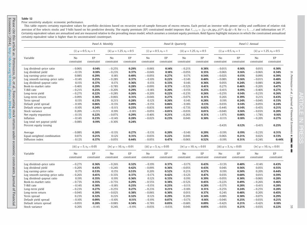
Table 12Prior sensitivity analysis: economic performance.
This table reports certainty equivalent values for portfolio decisions based on recursive out-of-sample forecasts of excess returns. Each period an investor with power utility and coefficient of relative riskaversion of five selects stocks and T-bills based on his predictive density. The equity premium (EP) constrained model imposes that r̂ τþ1jt ¼
R ðμþβxτÞpðμ; βjDt Þ dμ dβ40; for τ¼ 1;…; t and information set Dt .Certainty equivalent values are annualized and are measured relative to the prevailing mean model, which assumes a constant equity premium. Bold figures highlight instances in which the constrained annualizedcertainty equivalent value is higher than its unconstrained counterpart.
Panel A: Monthly Panel B: Quarterly Panel C: Annual
(i) ψ ¼ 0:5; v0 ¼ 1 (ii) ψ ¼ 1:25; v0 ¼ 0:5 (i) ψ ¼ 0:5; v0 ¼ 1 (ii) ψ ¼ 1:25; v0 ¼ 0:5 (i) ψ ¼ 0:5; v0 ¼ 1 (ii) ψ ¼ 1:25; v0 ¼ 0:5
Variable No EP No EP No EP No EP No EP No EPconstraint constraint constraint constraint constraint constraint constraint constraint constraint constraint constraint constraint
Log dividend–price ratio �0.06% 0.14% �0.25% 0.29% �0.06% 0.14% �0.21% 0.38% �0.01% 0.16% 0.01% 0.30%Log dividend yield �0.13% 0.18% �0.23% 0.37% �0.04% 0.18% �0.05% 0.35% �0.06% 0.16% �0.06% 0.34%Log earning–price ratio 0.08% 0.29% 0.18% 0.49% �0.05% 0.27% 0.17% 0.54% �0.02% 0.15% 0.09% 0.39%Log smooth earning–price ratio �0.14% 0.25% �0.28% 0.37% �0.10% 0.22% �0.14% 0.40% �0.08% 0.16% �0.01% 0.48%Log dividend–payout ratio 0.15% 0.37% 0.17% 0.36% 0.15% 0.33% 0.14% 0.36% 0.05% 0.24% �0.08% 0.28%Book-to-market ratio �0.46% 0.29% �0.78% 0.28% �0.09% 0.37% �0.52% 0.41% 0.27% 0.46% �0.20% 0.47%T-Bill rate �0.21% 0.25% �0.20% 0.29% �0.18% 0.20% �0.15% 0.25% �0.41% 0.19% �0.40% 0.27%Long-term yield �0.27% 0.22% �0.28% 0.26% �0.20% 0.22% �0.23% 0.26% �0.25% 0.14% �0.23% 0.26%Long-term return �0.09% 0.30% �0.06% 0.31% �0.04% 0.27% �0.07% 0.31% 0.26% 0.39% 0.21% 0.43%Term spread 0.15% 0.23% 0.21% 0.28% 0.12% 0.26% 0.14% 0.28% 0.19% 0.24% �0.04% 0.33%Default yield spread �0.10% 0.06% �0.13% 0.09% �0.15% 0.06% �0.18% 0.13% �0.03% 0.14% �0.05% 0.24%Default return spread �0.10% 0.24% �0.11% 0.25% �0.83% 0.01% �0.73% 0.02% �0.44% 0.14% �0.45% 0.21%Stock variance 0.20% �0.21% 0.19% �0.18% �0.05% �0.01% �0.03% 0.01% �0.04% 0.16% �0.03% 0.20%Net equity expansion �0.13% 0.22% �0.07% 0.29% �0.40% 0.21% �0.26% 0.31% �1.97% 0.08% �1.78% 0.16%Inflation �0.14% 0.23% �0.14% 0.28% �0.02% 0.23% 0.04% 0.30% �0.11% 0.18% �0.20% 0.27%Log total net payout yield �0.08% 0.19% �0.30% 0.24%Percent equity issuing �0.43% 0.12% �0.41% 0.25%
Average �0.08% 0.20% �0.13% 0.27% �0.13% 0.20% �0.14% 0.29% �0.19% 0.19% �0.23% 0.31%Equal-weighted combination 0.07% 0.21% 0.12% 0.31% �0.03% 0.22% 0.04% 0.28% �0.06% 0.21% 0.02% 0.33%Diffusion index �0.12% 0.37% �0.05% 0.44% �0.05% 0.47% �0.06% 0.52% �0.19% 0.31% �0.24% 0.44%
(iii) ψ ¼ 5; v0 ¼ 0:05 (iv) ψ ¼ 10; v0 ¼ 0:01 (iii) ψ ¼ 5; v0 ¼ 0:05 (iv) ψ ¼ 10; v0 ¼ 0:01 (iii) ψ ¼ 5; v0 ¼ 0:05 (iv) ψ ¼ 10; v0 ¼ 0:01
Variable No EP No EP No EP No EP No EP No EPconstraint constraint constraint constraint constraint constraint constraint constraint constraint constraint constraint constraint
Log dividend–price ratio �0.27% 0.36% �0.26% 0.32% �0.19% 0.37% �0.17% 0.43% �0.13% 0.40% �0.14% 0.43%Log dividend yield �0.20% 0.43% �0.24% 0.42% �0.09% 0.36% �0.05% 0.43% 0.04% 0.56% 0.05% 0.55%Log earning–price ratio 0.17% 0.53% 0.15% 0.53% 0.20% 0.52% 0.21% 0.57% 0.19% 0.50% 0.20% 0.44%Log smooth earning–price ratio �0.26% 0.41% �0.33% 0.37% �0.17% 0.42% �0.12% 0.47% 0.03% 0.60% 0.01% 0.59%Log dividend–payout ratio 0.19% 0.35% 0.19% 0.36% 0.12% 0.33% 0.19% 0.39% �0.05% 0.30% �0.06% 0.28%Book-to-market ratio �0.73% 0.35% �0.75% 0.29% �0.55% 0.38% �0.52% 0.45% �0.22% 0.49% �0.26% 0.46%T-Bill rate �0.14% 0.30% �0.18% 0.25% �0.15% 0.25% �0.11% 0.28% �0.37% 0.28% �0.41% 0.28%Long-term yield �0.23% 0.27% �0.25% 0.27% �0.23% 0.21% �0.18% 0.31% �0.25% 0.24% �0.25% 0.28%Long-term return �0.04% 0.39% �0.02% 0.38% �0.06% 0.30% 0.01% 0.37% 0.24% 0.48% 0.20% 0.45%Term spread 0.23% 0.32% 0.22% 0.32% 0.12% 0.29% 0.20% 0.34% �0.08% 0.30% �0.07% 0.29%Default yield spread �0.10% 0.09% �0.10% 0.11% �0.19% 0.07% �0.17% 0.16% �0.04% 0.25% �0.03% 0.21%Default return spread �0.05% 0.28% �0.08% 0.34% �0.78% 0.05% �0.68% 0.09% �0.42% 0.21% �0.42% 0.18%Stock variance 0.20% �0.14% 0.24% �0.19% �0.03% �0.03% 0.04% 0.05% �0.03% 0.21% �0.03% 0.22%
Pleasecite
thisarticle
as:Petten
uzzo,D
.,etal.,Forecastin
gstock
return
sunder
econom
iccon
straints.Jou
rnalofFin
ancial
Econom
ics(2014),h
ttp://d
x.doi.org/10.1016/j.jfin
eco.2014.07.015i
D.Pettenuzzo
etal./
Journalof
FinancialEconom
ics](]]]])
]]]–]]]
33

Net
equityex
pan
sion
�0.05
%0.27
%�0.04
%0.28
%�0.30
%0.30
%�0.22
%0.33
%�1.76
%0.22
%�1.75
%0.20
%Inflation
�0.10
%0.27
%�0.09
%0.31
%0.03
%0.27
%0.04
%0.33
%�0.20
%0.32
%�0.19
%0.29
%Lo
gtotalnet
pay
outyield
�0.25
%0.28
%�0.28
%0.28
%Pe
rcen
teq
uityissu
ing
�0.46
%0.22
%�0.52
%0.24
%
Ave
rage
�0.10
%0.30
%�0.11
%0.29
%�0.15
%0.27
%�0.10
%0.33
%�0.22
%0.35
%�0.23
%0.34
%Eq
ual-w
eigh
tedco
mbination
0.14
%0.34
%0.12
%0.30
%0.01
%0.29
%0.07
%0.36
%0.06
%0.36
%0.09
%0.35
%Diffusion
index
�0.06
%0.45
%�0.07
%0.43
%�0.06
%0.48
%�0.02
%0.55
%�0.23
%0.47
%�0.24
%0.46
%
Please cite this article as: Pettenuzzo, D., et al., Forecasting stocEconomics (2014), http://dx.doi.org/10.1016/j.jfineco.2014.07.01
D. Pettenuzzo et al. / Journal of Financial Economics ] (]]]]) ]]]–]]]34
rise to dynamic learning effects that can shift the entirepredictive distribution for the equity premium evenin situations in which no such change is observed undera conventional unconstrained model.
Imposing economic constraints on the equity premiumforecast improves the predictive accuracy for nearly all ofthe prediction models we consider. Moreover, the benefitsfrom the economic constraints seem to improve, thelonger the forecast horizon. In turn, when used to selectportfolio weights, the constrained forecasts are found toyield higher certainty equivalent returns than their uncon-strained counterparts.
Appendix A
This Appendix explains how we obtain parameterestimates for the models described in Section 2, and howwe use these to generate predictive densities for excessreturns. We begin by discussing the unconstrained modelin Eq. (1) and then turn to the models that incorporate theconstraints in Eqs. (2) and (8).
A.1. No constraints
In the unconstrained case, the goal is to obtain drawsfrom the joint posterior distribution pðμ;β;σ�2
ε jDtÞ withDt denoting all information available up to time t. Combin-ing the priors in Eqs. (9)–(13) with the likelihood functionyields the following conditional posteriors:
μβ
" #σ�2ε ;Dt �Nðb;V Þ
��� ðA:1Þ
and
σ�2ε jμ;β;Dt � Gðs�2; vÞ; ðA:2Þ
where
V ¼ V �1þσ�2ε ∑
t�1
τ ¼ 1zτz0τ
� ��1
;
b ¼ V V �1bþσ�2ε ∑
t�1
τ ¼ 1zτrτþ1
� �;
v ¼ v0þðt�1Þ; ðA:3Þ
zτ ¼ ð1xτÞ0, and
s2 ¼∑t�1τ ¼ 1ðrτþ1�μ�βxτÞ2þðs2r;t � v0ðt�1ÞÞ
v: ðA:4Þ
A Gibbs sampler algorithm can be used to iterate back andforth between Eqs. (A.1) and (A.2), yielding a series ofdraws for the parameter vector ðμ;β;σ�2
ε Þ. Draws from thepredictive density pðrtþ1jDtÞ can then be obtained bynoting that
pðrtþ1jDtÞ ¼Zμ;β;σ � 2
ε
pðrtþ1jμ;β;σ�2ε ;DtÞpðμ;β;σ�2
ε jDtÞ dμ dβ dσ�2ε :
ðA:5Þ
k returns under economic constraints. Journal of Financial5i

D. Pettenuzzo et al. / Journal of Financial Economics ] (]]]]) ]]]–]]] 35
A.2. Equity premium constraints
The approach used for the unconstrained model alsoworks when EP constraints are imposed subject to simplyintroducing an accept-reject step in Eq. (20):
μβ
" #σ�2ε ;Dt �Nðb;V Þ � μ;βAAt ;
���σ�2ε jμ;β;Dt � Gðs�2; vÞ; ðA:6Þ
with At defined in Eq. (18), and, once again, using Eq. (A.5)to draw from the predictive density pðrtþ1jDtÞ.
A.3. Conditional Sharpe ratio constraints
To obtain draws from the joint posterior distributionpðμ;β;ht ;σ�2
ξ jDtÞ under the SR constraints, we use theGibbs sampler to draw recursively from three conditionaldistributions
1.
stat
PE
pðht jμ;β;σ�2ξ ;DtÞ
t
2. pðμ;βjh ;σ�2ξ ;DtÞt t
3. pðσ�2ξ jμ;β;h ;D ÞWe simulate from each of these blocks as follows.Starting with pðht jμ;β;σ�2
ξ ;DtÞ; we employ the algorithmof Kim, Shephard, and Chib (1998). Define rnτþ1 ¼rτþ1�μ�βxτ and note that rnτþ1 is observable conditionalon μ;β. Next, rewriting Eq. (5) as
rnτþ1 ¼ expðhτþ1Þuτþ1: ðA:7Þ
Squaring and taking logs on both sides of Eq. (A.7) yields anew state space system that replaces Eqs. (5)–(6) with
rnnτþ1 ¼ 2hτþ1þunn
τþ1 ðA:8Þ
and
hτþ1 ¼ hτþξτþ1; ðA:9Þ
where rnnτþ1 ¼ lnðr2τþ1Þ and unn
τþ1 ¼ lnðu2τþ1Þ, with unn
τ inde-pendent of ξs for all τ and s. Because unn
tþ1 � lnðχ21Þ, we
cannot resort to standard Kalman recursions and simula-tion algorithms such as those in Carter and Kohn (1994) orDurbin and Koopman (2002). To obviate this problem,Kim, Shephard, and Chib (1998) employ a data augmenta-tion approach and introduce a new state variable sτþ1,τ¼ 1;…; t�1, turning their focus on drawing frompðht jμ;β;σ�2
ξ ; st ;DtÞ instead of pðht jμ;β;σ�2ξ ;DtÞ:23 The
introduction of the state variable sτþ1 allows us to rewritethe linear non-Gaussian state space representation inEqs. (A.8)–(A.9) as a linear Gaussian state space model,making use of the approximation
unn
τþ1 � ∑7
j ¼ 1qjf Nðmj�1:2704; v2j Þ; ðA:10Þ
wheremj, vj2, and qj, j¼ 1;2;…;7, are constants specified in
Kim, Shephard, and Chib (1998) and thus need not be
23 Here st ¼ fs2 ; s3;…; stg denotes the history up to time t of the newe variable s.
lease cite this article as: Pettenuzzo, D., et al., Forecasting stocconomics (2014), http://dx.doi.org/10.1016/j.jfineco.2014.07.01
estimated. In turn, Eq. (A.10) implies
unn
τþ1jsτþ1 ¼ j�Nðmj�1:2704; v2j Þ; ðA:11Þ
where each state has probability
Prðsτþ1 ¼ jÞ ¼ qj: ðA:12Þ
Conditional on st, we can rewrite the nonlinear state spacesystem as
rnnτþ1 ¼ 2hτþ1þeτþ1;
hτþ1 ¼ hτþξτþ1; ðA:13Þ
where eτþ1 �Nðmj�1:2704; v2j Þ with probability qj. Forthis linear Gaussian state space system, we can use thealgorithm of Carter and Kohn (1994) to draw the wholesequence of stochastic volatilities, ht.
Finally, conditional on the whole sequence ht, draws forthe sequence of states st can easily be obtained, noting that
Prðsτþ1 ¼ j rnnτþ1;hτþ1�� �¼ f Nðrnnτþ1j2hτþ1�mjþ1:2704; v2j Þ
∑7l ¼ 1f Nðrnnτþ1j2hτþ1�mlþ1:2704; v2l Þ
:
ðA:14ÞMoving on to pðμ;βjht ;σ�2
ξ ;DtÞ, conditional on ht it isstraightforward to draw μ;β, and apply standard results.Specifically,
μβ
" #ht ;σ�2
ξ ;Dt �Nðb;V Þ � μ;βA ~At ;��� ðA:15Þ
where ~At is defined in (19), with
V ¼ V �1þ ∑t�1
τ ¼ 1
1expðhτþ1Þ2
zτz0τ
( )�1
;
b ¼ V V �1bþ ∑t�1
τ ¼ 1
1expðhτþ1Þ2
zτrτþ1
( ):
Next, the posterior distribution for pðσ�2ξ jμ;β;ht ;DtÞ is
readily available as,
σ�2ξ jμ;β;ht ;Dt � G
kξþ∑t�1τ ¼ 2ðhτþ1�hτÞ2
t�1
" #�1
; t�1
0@ 1A:
ðA:16ÞFinally, draws from the predictive density pðrtþ1jDtÞ can beobtained by noting than
pðrtþ1jDtÞ ¼Zμ;β;ht þ 1 ;σ � 2
ξ
pðrtþ1jhtþ1;μ;β;ht ;σ�2
ξ ;DtÞ
�pðhtþ1jμ;β;ht ;σ�2ξ ;DtÞ
�pðμ;β;ht ;σ�2ξ jDtÞ dμ dβ dhtþ1 dσ�2
ξ : ðA:17Þ
The first term in the integral above, pðrtþ1jhtþ1;μ;β;h
t ;σ�2ξ ;DtÞ, represents the period tþ1 predic-
tive density of excess returns, treating model parametersas if they were known with certainty, and so is straightfor-ward to calculate. The second term in the integral,pðhtþ1jμ;β;ht ;σ�2
ξ ;DtÞ, reflects how period tþ1 volatilitymay drift away from ht over time. Finally, the last term inthe integral, pðμ;β;ht ;σ�2
ξ jDtÞ, measures parameter uncer-tainty in the sample.
k returns under economic constraints. Journal of Financial5i

D. Pettenuzzo et al. / Journal of Financial Economics ] (]]]]) ]]]–]]]36
To obtain draws for pðrtþ1jDtÞ, we proceed in threesteps:
1.
PE
Simulate from pðμ;β;ht ;σ�2ξ jDtÞ: draws from
pðμ;β;ht ;σ�2ξ jDtÞ are obtained from the Gibbs sampling
algorithm described above.
2. Simulate from pðhtþ1jμ;β;ht ;σ�2ξ ;DtÞ: having pro-cessed data up to time t, the next step is to simulatethe future volatility, htþ1. For a given ht and σ�2
ξ , notethat μ and β and the history of volatilities up to tbecome redundant, i.e., pðhtþ1jμ;β;ht ;σ�2
ξ ;DtÞ ¼pðhtþ1jht ;σ�2
ξ ;DtÞ. Note also that (6) along with thedistributional assumptions made with regards to ξτþ1imply that
htþ1jht ;σ�2ξ ;Dt �Nðht ;σ2
ξÞ: ðA:18Þ
3.
Simulate from pðrtþ1jhtþ1;μ;β;ht ;σ�2ξ ;DtÞ: For a givenhtþ1, μ; and β; note that ht and σ�2
ξ become redundant,i.e., pðrtþ1jhtþ1;μ;β;h
t ;σ�2ξ ;DtÞ ¼ pðrtþ1jhtþ1;μ;β;DtÞ:
Then use the fact that
rtþ1jhtþ1;μ;β;Dt �Nðμþβxt ; expðhtþ1ÞÞ: ðA:19Þ
References
Andersen, T.G., Bollerslev, T., Christoffersen, P.F., Diebold, F.X., 2006.Volatility and correlation forecasting. Handbook of Economic Fore-casting, vol. 1. Elsevier, North-Holland, pp. 777–878.
Ang, A., Piazzesi, M., 2003. A no-arbitrage vector autoregression of termstructure dynamics with macroeconomic and latent variables. Journalof Monetary Economics 50 (4), 745–787.
Aït-Sahalia, Y., Brandt, M.W., 2001. Variable selection for portfolio choice.The Journal of Finance 56 (4), 1297–1351.
Avramov, D., Wermers, R., 2006. Investing in mutual funds when returnsare predictable. Journal of Financial Economics 81 (2), 339–377.
Banbura, M., Giannone, D., Reichlin, L., 2010. Large Bayesian vector autoregressions. Journal of Applied Econometrics 25 (1), 71–92.
Barberis, N., 2000. Investing for the long run when returns are predict-able. The Journal of Finance 55 (1), 225–264.
Bossaerts, P., Hillion, P., 1999. Implementing statistical criteria to selectreturn forecasting models: what do we learn?. Review of FinancialStudies 12 (2), 405–428.
Boudoukh, J., Richardson, M., Smith, T., 1993. Is the ex ante risk premiumalways positive?: a new approach to testing conditional asset pricingmodels Journal of Financial Economics 34 (3), 387–408.
Brandt, M.W., 2010. Portfolio Choice Problems. Handbook of FinancialEconometrics, vol. 1. Elsevier, North-Holland pp. 269–336.
Brennan, M.J., Schwartz, E.S., Lagnado, R., 1997. Strategic asset allocation.Journal of Economic Dynamics and Control 21, 1377–1403.
Campbell, J., Shiller, R., 1988. The dividend–price ratio and expectationsof future dividends and discount factors. Review of Financial Studies1 (3), 195–228.
Campbell, J.Y., 1987. Stock returns and the term structure. Journal ofFinancial Economics 18 (2), 373–399.
Campbell, J.Y., Thompson, S.B., 2008. Predicting excess stock returns outof sample: can anything beat the historical average? Review ofFinancial Studies 21 (4), 1509–1531.
Campbell, J.Y., Viceira, L.M., 1999. Consumption and portfolio decisionswhen expected returns are time varying. The Quarterly Journal ofEconomics 114 (2), 433–495.
Carter, C.K., Kohn, R., 1994. On Gibbs sampling for state space models.Biometrika 81 (3), 541–553.
Clark, T.E., West, K.D., 2007. Approximately normal tests for equalpredictive accuracy in nested models. Journal of Econometrics 138(1), 291–311.
Cochrane, J.H., 2001. Asset Pricing. Princeton University Press, USA.Cochrane, J.H., Saa-Requejo, J., 2000. Beyond arbitrage: good-deal asset
price bounds in incomplete markets. Journal of Political Economy 108(1), 79–119.
lease cite this article as: Pettenuzzo, D., et al., Forecasting stocconomics (2014), http://dx.doi.org/10.1016/j.jfineco.2014.07.01
Diebold, F.X., 2012. Comparing predictive accuracy, twenty years later: apersonal perspective on the use and abuse of Diebold–Mariano tests.Working paper. University of Pennsylvania.
Durbin, J., Koopman, S.J., 2002. A simple and efficient simulationsmoother for state space time series analysis. Biometrika 89 (3),603–615.
Efron, B., 2010. Large-Scale Inference: Empirical Bayes Methods forEstimation, Testing, and Prediction. Cambridge University Press, UK.
Fama, E.F., French, K.R., 1988. Dividend yields and expected stock returns.Journal of Financial Economics 22 (1), 3–25.
Fama, E.F., French, K.R., 1989. Business conditions and expected returnson stocks and bonds. Journal of Financial Economics 25 (1), 23–49.
Ferson, W.E., Harvey, C.R., 1991. The variation of economic risk premiums.Journal of Political Economy 99 (2), 385–415.
Ferson, W.E., Schadt, R.W., 1996. Measuring fund strategy and perfor-mance in changing economic conditions. The Journal of Finance 51(2), 425–461.
Goyal, A., Welch, I., 2003. Predicting the equity premium with dividendratios. Management Science 49 (5), 639–654.
Henkel, S.J., Martin, J.S., Nardari, F., 2011. Time-varying short-horizonpredictability. Journal of Financial Economics 99 (3), 560–580.
Jobson, J.D., Korkie, B.M., 1981. Performance hypothesis testing with theSharpe and Treynor measures. The Journal of Finance 36 (4), 889–908.
Kadiyala, K.R., Karlsson, S., 1997. Numerical methods for estimation andinference in Bayesian var-models. Journal of Applied Econometrics 12(2), 99–132.
Kandel, S., Stambaugh, R.F., 1996. On the predictability of stock returns:an asset-allocation perspective. The Journal of Finance 51 (2),385–424.
Keim, D.B., Stambaugh, R.F., 1986. Predicting returns in the stock andbond markets. Journal of Financial Economics 17 (2), 357–390.
Kelly, B.T., Pruitt, S., 2013. Market expectations in the cross-section ofpresent values. Journal of Finance 68 (5), 1721–1756.
Kim, S., Shephard, N., Chib, S., 1998. Stochastic volatility: likelihoodinference and comparison with arch models. The Review of EconomicStudies 65 (3), 361–393.
Koop, G., 2003. Bayesian Econometrics. John Wiley & Sons, Ltd, England.Lamont, O., 1998. Earnings and expected returns. The Journal of Finance
53 (5), 1563–1587.Lettau, M., Ludvigson, S., 2001. Consumption, aggregate wealth, and
expected stock returns. The Journal of Finance 56 (3), 815–849.Lettau, M., Ludvigson, S.C., 2010. Measuring and Modeling Variation in
the Risk-return Trade-off. Handbook of Financial Econometrics, vol. 1.Elsevier, North-Holland pp. 617–690.
Lettau, M., Van Nieuwerburgh, S., 2008. Reconciling the return predict-ability evidence. Review of Financial Studies 21 (4), 1607–1652.
Lettau, M., Wachter, J.A., 2007. Why is long-horizon equity less risky? Aduration-based explanation of the value premium. The Journal ofFinance 62 (1), 55–92.
Lettau, M., Wachter, J.A., 2011. The term structures of equity and interestrates. Journal of Financial Economics 101 (1), 90–113.
Ludvigson, S.C., Ng, S., 2007. The empirical risk–return relation: a factoranalysis approach. Journal of Financial Economics 83 (1), 171–222.
MacKinlay, A., 1995. Multifactor models do not explain deviations fromthe capm. Journal of Financial Economics 38 (1), 3–28.
MacKinlay, A.C., Pastor, L., 2000. Asset pricing models: implications forexpected returns and portfolio selection. The Review of FinancialStudies 13 (4), 883–916.
Neely, C., Rapach, D.E., Tu, J., Zhou, G., 2012. Forecasting the equity riskpremium: the role of technical indicators. Federal Reserve Bank of St.Louis working paper.
Ostdiek, B., 1998. The world ex ante risk premium: an empiricalinvestigation. Journal of International Money and Finance 17 (6),967–999.
Pastor, L., Stambaugh, R.F., 2009. Predictive systems: living with imper-fect predictors. The Journal of Finance 64 (4), 1583–1628.
Pastor, L., Stambaugh, R.F., 2012. Are stocks really less volatile in the longrun? The Journal of Finance 67 (2), 431–478.
Paye, B.S., Timmermann, A., 2006. Instability of return prediction models.Journal of Empirical Finance 13 (3), 274–315.
Pesaran, M.H., Timmermann, A., 1995. Predictability of stock returns:robustness and economic significance. The Journal of Finance 50 (4),1201–1228.
Poirier, D.J., 1995. Intermediate Statistics and Econometrics: A Compara-tive Approach. MIT Press, USA.
Polk, C., Thompson, S., Vuolteenaho, T., 2006. Cross-sectional forecasts ofthe equity premium. Journal of Financial Economics 81 (1), 101–141.
k returns under economic constraints. Journal of Financial5i

D. Pettenuzzo et al. / Journal of Financial Economics ] (]]]]) ]]]–]]] 37
Pontiff, J., Schall, L.D., 1998. Book-to-market ratios as predictors of marketreturns. Journal of Financial Economics 49 (2), 141–160.
Rapach, D.E., Strauss, J.K., Zhou, G., 2010. Out-of-sample equity premiumprediction: combination forecasts and links to the real economy.Review of Financial Studies 23 (2), 821–862.
Rapach, D.E., Zhou, G., 2013. Forecasting stock returns. In: Elliot, G.,Timmermann, A. (Eds.), Handbook of Economic Forecasting, vol. 2. ,North-Holland.
Ross, S.A., 1976. The arbitrage theory of capital asset pricing. Journal ofEconomic Theory 13 (3), 341–360.
Ross, S.A., 2005. Neoclassical Finance. Princeton University Press, USA.Shanken, J., Tamayo, A., 2012. Payout yield, risk, and mispricing: a
Bayesian analysis. Journal of Financial Economics 105 (1), 131–152.Stock, J.H., Watson, M.W., 2006. Forecasting with many Predictors.
Handbook of Economic Forecasting, vol. 1. Elsevier, North-Hollandpp. 515–554.
Please cite this article as: Pettenuzzo, D., et al., Forecasting stocEconomics (2014), http://dx.doi.org/10.1016/j.jfineco.2014.07.01
Wachter, J.A., Warusawitharana, M., 2009. Predictable returns and assetallocation: should a skeptical investor time the market?. Journal ofEconometrics 148 (2), 162–178.
Welch, I., Goyal, A., 2008. A comprehensive look at the empiricalperformance of equity premium prediction. Review of FinancialStudies 21 (4), 1455–1508.
Xia, Y., 2001. Learning about predictability: the effects of parameteruncertainty on dynamic asset allocation. The Journal of Finance 56(1), 205–246.
Zhou, G., 2010. How much stock return predictability can we expect froman asset pricing model? Economics Letters 108 (2), 184–186.
k returns under economic constraints. Journal of Financial5i