forecasting stock market trends by …ijecm.co.uk/wp-content/uploads/2016/06/4614.pdf ·...

International Journal of Economics, Commerce and Management United Kingdom Vol. IV, Issue 6, June 2016

Licensed under Creative Common Page 220

http://ijecm.co.uk/ ISSN 2348 0386

FORECASTING STOCK MARKET TRENDS BY LOGISTIC

REGRESSION AND NEURAL NETWORKS

EVIDENCE FROM KSA STOCK MARKET

Makram Zaidi

College of administrative sciences, Najran University, Kingdom of Saudi Arabia

[email protected]

Amina Amirat

College of administrative sciences, Najran University, Kingdom of Saudi Arabia

Abstract

Estimating stock market trends is very important for investors to act for future. Kingdom of Saudi

Arabia (KSA) stock market is evolving rapidly; so the objective of this paper is to forecast the

stock market trends using logistic model and artificial neural network. Logistic model is a variety

of probabilistic statistical classification model. It is also used to predict a binary response from

a binary predictor. Artificial neural networks are used for forecasting because of their capabilities

of pattern recognition and machine learning. Both methods are used to forecast the stock prices

of upcoming period. The model has used the preprocessed data set of closing value of TASA

Index. The data set encompassed the trading days from 5th April, 2007 to 1st January, 2015.

With logistic regression it may be observed that four variables i.e. open price, higher price, lower

price and oil can classify up to 81.55% into two categories up and down. While with neural

networks The prediction accuracy of the model is high both for the training data (84.12%) and

test data (81.84%).

Keywords: Forecasting, Logistic Model, Neural Networks, Stock Index, Trends

http://ijecm.co.uk/

http://ijecm.co.uk/

http://en.wikipedia.org/wiki/Statistical_classification

http://en.wikipedia.org/wiki/Binary_classification

International Journal of Economics, Commerce and Management, United Kingdom

Licensed under Creative Common 21

INTRODUCTION

Recently predicting stock market trends is gaining more consideration, perhaps because of the

fact that if the trend of the market is successfully forecasted the traders may be well directed.

The profitability of trading in the stock market to a large extent rest on the predictability. More

over the forecast trends of the market will support the regulators of the market in taking

corrective measures.

Estimating in stock market has been constructed on traditional statistical forecast

methods for long time. Linear models have been the midpoint of such traditional methods. But,

these methods have seldom demonstrated successful due to the existence of noise and non-

linearity in historical data. The successful use of nonlinear methods in other arenas of

investigation has flashed the optimisms of financials. Non linear methods propose an advanced

approach of perceiving stock prices, and it offers novel methods for practically assessing their

nature.

The objective of this paper is to forecast the stock market trends using logistic model

and artificial neural network. Logistic model is a variety of probabilistic statistical

classification model. It is also used to predict a binary response from a binary predictor. Artificial

neural networks are used for forecasting because of their capabilities of pattern recognition and

machine learning. Both methods are used to forecast the stock prices of upcoming period. The

model has used the preprocessed data set of closing value of TASA Index. The data set

encompassed the trading days from 5thApril, 2007 to 1st January; 2015.Both methods give us

estimation with up to 80% accuracy.

This paper is structured in four sections. The first one introduce the study, in the second

we review literature linked to our paper, then we explain methodology of research and present

results, the forth section concludes the paper.

LITERATURE REVIEW

Logistic Regression is a multivariate analysis model (Lee, 2004) very useful for prediction. The

applications of this model in the area of finance are growing rapidly. Many researchers

employed the multivariate discriminant analysis prediction model. Altman is the pioneer in the

year 1968 while logistic regression was used by the Ohlson in 1980. The first study on

prediction focuses on classifying companies as either non-defaulters or defaulters.

In forecasting bankruptcy and financial distress, logistic regression was applied by

Ohlson (1980) and then by Zavgren (1985) and other researchers. Logistic regression technique

yields coefficients for each independent variable based on a sample of data (Huang, Chai and

Peng, 2007). Logistic regression models with more than one explanatory variable are applied in

http://ijecm.co.uk/




http://en.wikipedia.org/wiki/Binary_classification

© Zaidi & Amirat


practice (Haines and others, 2007, Pardo, Pardo and Pardo, 2005). The benefit of logistic

regression is that variables may be either discrete or continuous; they do not necessarily have

normal distributions (Lee, 2004).

Neural networks have showed to be a talented area of investigation in the field of

finance. Neural network practices in finance comprise assessing the risk of mortgage loans

(Collins, Ghosh and Scofield, 1988), scoring the value of company bonds (Dutta & Shekhar,

1988), forecasting financial default (Altman, et.al., 1994), ranking of credit card users (Suan &

Chye, 1997) and expecting bond ratings (Hatfield & White, 1996). Neural networks are also

applied in areas such as valuing of derivatives (Hutchinson, 1994, Refenes, 1997, McCluskey,

1993), etc.

Actually, numerous practitioners in the stock market have also understood the likely of

neural networks. Hadavandi, Shavandi et al. (2010) show an combined approach founded on

artificial neural networks (ANN) and genetic fuzzy systems (GFS) for building a stock price

predicting expert system. Kara, Acar Boyacioglu et al (2010) used artificial neural networks and

support vector machines in expecting direction of stock price index of the Istanbul Stock

Exchange. Shen, Guo et al. (2010) employed a radial basis function neural network and the

artificial fish swarm algorithm (AFSA) to estimate the stock indices of the Shanghai Stock

Exchange.

Additionally, Chih-Fong and Yu-Chieh (2010) jointed multiple feature assortment

methods to recognize more representative variables for improved forecast for investors. In

particular, they used: Genetic Algorithms (GA), Principal Component Analysis (PCA) and

decision trees (CART). Esfahanipour and Aghamiri (2010) developed Neuro-Fuzzy Inference

System implemented on a Takagi–Sugeno–Kang (TSK) for stock price prediction.

Also, Ni, Ni et al (2011) hybridizes fractal feature selection method and support vector machine

to predict the direction of daily stock price index. Bajestani and Zare (2011) offered a new

method to predict TAIEX based on a high-order type 2 fuzzy time series. The results designated

that the proposed model beats previous studies.

RESEARCH METHODOLOGY

The data consists of daily index values of the Saudi stock market (TASA). The period under

consideration is 05/04/2008to 01/01/2015. The data set consists of 1342 data points. The data

has been obtained from the official web site of Saudi stock market that provides daily stock

market data. The entire analysis has been done basically on the daily returns of the stock

market index TASA.



Application of Logistic Regression

Logistic regression is used in our study because we assume that the relation between variables

is non-linear. Also this type of regression is preferred when the response variable is binary

which means that can take only two values 1 or 0.

Logistic regression could forecast the likelihood, or the odds ratio, of the outcome based

on the predictor variables, or covariates. The significance of logistic regression can be

evaluated by the log likelihood test, given as the model chi-square test, evaluated at the p <

0.05 level, or the Wald statistic. Logistic regression has the advantage of being less affected

than discriminant analysis when the normality of the variable cannot be assumed.

It has the capacity to analyze a mix of all types of predictors [Hair, 1995]. Logistic

regression, which assumes the errors are drawn from a binomial distribution, is formulated to

predict and explain a binary categorical variable instead of a metric measure. In logistic

regression, the dependent variable is a log odd or logit, which is the natural log of the odds.

In the logistic regression model, the relationship between Z and the probability of the

event of interest is described by this link function.

𝑝𝑖 =𝑒𝑧𝑖

1+𝑒𝑧𝑖=

1

1+𝑒−𝑧𝑖

𝑧𝑖 = 𝑙𝑜𝑔 𝑝𝑖 1 − 𝑝𝑖

Where

pi is the probability the ith case experiences the event of interest

zi is the value of the unobserved continuous variable for the ith case

The z value is the odds ratio. It is expressed by

𝑧𝑖 = 𝑐 + 𝛽1𝑥𝑖1 + 𝛽2𝑥𝑖2 + ⋯ + 𝛽𝑝𝑥𝑖𝑝

Where

𝑥𝑖𝑗 is the jth predictor for the ith case

𝛽𝑗 is the jth coefficient

P is the number of predictors

βs are the regression coefficients that are estimated through an iterative maximum likelihood

method. However, because of the subjectivity of the choice of these misclassification costs in

practice, most researchers minimize the total error rate and, hence, implicitly assume equal

costs of type I and type II errors [Ohlson, 1980; Zavgren, 1985].

In order to carry out logistic regression analysis, first a method is needed for classifying

returns as a “1” or “0” for a given day. In this study we use a method that is simple and

objective, if the value of a return in day j is above the return in day j-1, it is noted as a “1”;

otherwise, it is classified as a “0”.

http://ijecm.co.uk/

© Zaidi & Amirat


The return was calculated using the following formula:

𝑟𝑒𝑡𝑢𝑟𝑛 =𝑝𝑗 − 𝑝𝑗−1

𝑝𝑗−1× 100

Where:

𝑝𝑗 is the closing price for day j

𝑝𝑗−1is the closing price for day j-1

As mentioned, the study contains 1678 data where 1342 are used for estimating and 336 used

for validating the model. For variables we have the market return as dependent variable and five

independent variables. One of them is fundamental variable oil, and the reminders are technical

variables: open price, higher price, lower price and turnover.

We conduct the logistic regression in two steps. The first called general model where we

introduced all our independent variables. The second is called the reduced model where we use

only the significant variables of the general model. The estimation is done using the software

Eviews 7.

ANALYSIS AND FINDINGS

Table 1: General Model Results

Variables Coefficient Std. error z-statistic Prob.

Constant 0.178794 0.076468 2.338142 0.0194

Higher price 186.6705 17.63165 10.58724 0.0000

Lower price 191.2550 14.72109 12.99190 0.0000

Oil 9.394324 3.596176 2.612309 0.0090

Open price -189.6573 13.24681 -14.31721 0.0000

Turnover 0.854115 0.492648 1.733722 0.0830*

(*): is significantly non-significant at 5% level

The final logistic regression equation is estimated in general model by using the maximum

likelihood estimation:

Z = 0.178794 + 186.6705 * Higher + 191.2550 * Lower + 9.394324 * Oil - 189.6573 * Open +

0.854115 * Turnover

Where,

Z = log (p /1 – p)

and „p‟ is the probability that the variable is 1.

We note that the statistic LR is equal to 716.5421. This statistic suppose in the null hypothesis

that all coefficients are equal to zero except the constant. Here we reject this hypothesis with

zero probability to be wrong. This means that our model is globally significant. To enforce the



results of the LR test we make the wald test which study the same hypothesis. We found F-

statistics equal to 57.49 (prob =0) and chi-square equal to 287.48 (prob=0). So we reject the null

hypothesis.

Also we have McFadden R-squared equal to 0.387 which is between 0.2 and 0.4 and

that means the explicative power of the model is excellent.

Regarding the results of this model, the variable lower price has the higher influence on

the market return and is more important in prediction among the technical variables chose in our

estimation while the variable turnover is significantly non-significant so it will be removed in the

next step which is the reduced model.

Table 2: Reduced Model Results

Variables Coefficient Std. error z-statistic Prob.

Constant 0.173331 0.076299 2.271736 0.0231

Higher price 196.5624 16.86996 11.65162 0.0000

Lower price 187.9323 14.57554 12.89367 0.0000

Oil 9.484048 3.582098 2.647623 0.0081

Open price -191.7596 13.23194 -14.49217 0.0000

The final logistic regression equation is estimated in a reduced model by using the maximum

likelihood estimation:

Z = 0.173331 + 196.5624 * Higher + 187.9323 * Lower + 9.484048 * Oil - 191.7596 * Open

Where

Z = log (p /1 – p)

and „p‟ is the probability that the variable is 1.

In this estimation the higher price has more influence on the market return and can be more

significant in forecasting stock return.

We note that the statistic LR is equal to 713.5310. This statistic suppose in the null

hypothesis that all coefficients are equal to zero except the constant. Here we reject this

hypothesis with zero probability to be wrong. This means that our model is globally significant.

To enforce the results of the LR test we make the Wald test which study the same hypothesis.

We found F-statistics equal to 71.30506 (prob =0) and chi-square equal to 285.2202 (prob=0).

So we reject the null hypothesis.

To measure the quality of our model we calculate McFadden Rsquare, Cox & Snell

Rsquare, max Rsquare and Nagelkerke adjusted Rsquare. The results are:

http://ijecm.co.uk/

© Zaidi & Amirat


Table 3: Measuring the Quality of Models

Measure Complete model Reduced model

McFadden Rsquare 0.3870 0.3854

Cox &Snell Rsquare 0.4136 0.4123

Max Rsquare 0.5707 0.5716

Nagelkerke adjusted Rsquare 0.7236 0.7212

These indicators show at first that the explicative power still the same after moving to the

reduced model. Secondly, the Nagelkerke adjusted Rsquare is close to 1 which indicate that the

significant power of our models is great.

We can also scan the information criteria that furnish a measure of the quality of information

given by the model. We can find this criteria by a combination between the log likelihood, the

number of observations and the number of variables. These criteria are: AKAIKE, Schwarz and

Hannan-Quin.

Table 4: Measuring the Quality of Information Given by Models


Akaike info criterion 0.854574 0.855328

Schwarz criterion 0.877832 0.874709

Hannan-Quinn citerions 0.863287 0.862588

We note from table (4) that the criteria is the same for Akaike while Schwarz and Hannan-Quinn

decreased in the reduced model which means that the later give better information.

The last step to validate the reduced model is to check its predictive quality. For this

reason, we will make the test of Goodness-of-Fit Evaluation for Binary Specification: Andrews

and Hosmer-Lemeshow Tests. The results are:

Table 5: Measuring the Predictive Quality of Models


H-L Statistic 111.0267 112.9785

Prob. Chi-Sq(8) 0.0000 0.0000

Andrews Statistic 65.3223 64.2026

Prob. Chi-Sq(10) 0.0000 0.0000

This test reflect that the reduced model give a better predictive quality with zero probability of

error. So, we will estimate the value of y using the reduced model for our 1342 observation. The

test of Expectation-Prediction Evaluation for Binary Specification shows the results as presented

in the table 6.



Table 6: Expectation-Prediction Evaluation

Measure Correct (%) Wrong (%)

Y=1 86.50 13.50

Y=0 80.68 19.32

Total 83.83 16.17

With the reduced model, 83.83% of estimation are correct. So we validate this model and we

can now interpret the coefficient and make an estimation of the reminder data.

Here, we will speak about the marginal effect of variables. The marginal effect for jth

explicative variable 𝑥𝑖 𝑗

is defined as :

𝜕𝑝𝑖

𝜕𝑥𝑖 𝑗

= 𝑓 𝑥𝑖𝛽 . 𝛽𝑗 =𝑒𝑥𝑖𝛽

1 + 𝑒𝑥𝑖𝛽 2𝛽𝑗

Because of the sign of 𝑓 𝑥𝑖𝛽 is always positive, so the sign of this derivate is the same of the

coefficient. So the positive sign indicate an increase in the probability of y to be equal to 1 which

is the case for variables: higher price, lower price, and oil. While a negative sign reflect a

decrease in this probability which the case for the variable open price.

For more explanation we calculate the elasticity 𝜀𝑝𝑖 𝑥𝑖

𝑗 as the variation in percentage of

the probability 𝑝𝑖 that 𝑦𝑖 = 1 occurs due to a variation of 1% of the jth explicative variable 𝑥𝑖 𝑗

.

Elasticity is defined as:

∀𝑖 ∈ 1, 𝑁 𝜀𝑝𝑖 𝑥𝑖

𝑗 =

𝑥𝑖 𝑗

𝛽𝑗

1 + 𝑒𝑥𝑝𝑥𝑖𝛽

Table 7: Elasticity of Variables in Complete Model

Variables Higher price Lower price Oil Open price

Elasticity -1.04% -0.93% -0.021% 0.86%

If these variables change by 1% the occurrence probability of 𝑦𝑖 = 1 decrease for all variables

except the open price.

Using this result we will estimate the value of our dependent variable for the left 336 data

in order to test the performance of our model. The results are shown in the following table:

Table 8: Testing the Performance of the Model

Prediction Number Percentage

Correct 274 81.55%

Wrong 62 18.45%

Total 336 100%

http://ijecm.co.uk/

© Zaidi & Amirat


From the table above we can deduce that the accuracy of our model is of 81.55% which is very

important and can help investor to implement the best investment strategy. 3-2- Application of

artificial neural network

A neural network is a great data modeling device that is able to capture and represent

complex input/output relations. The inspiration for the development of neural network

technology stemmed from the wish to develop an artificial system that could make "intelligent"

tasks similar to those done by the human brain. Neural networks resemble the human brain in

the following two ways: At first, a neural network acquires knowledge through learning and

secondly, a neural network's knowledge is stored within inter-neuron connection strengths

known as synaptic weights.

From a very broad perspective, neural networks can be used for financial decision

making in one of the three ways:

1. It can be provided with inputs, which enable it to find rules relating the current state of the

system being predicted to future states.

2. It can have a window of inputs describing a fixed set of recent past states and relate those to

future states.

3. It can be designed with an internal state to enable it to learn the relationship of an in definitely

large set of past inputs to future states, which can be accomplished via recurrent

connections.

In this paper, one model of neural network is selected among the main network architectures

used in finance. The basis of the model is neuron structure as shown in Fig. 1.

Figure 1: Neuron model

X11

X21

Xm1

Wk11

Wk21

Wkm

1

𝛴1

bk1

f(vk)f ykf vkf

Inputf

weightsf

Biasf

Activation functionf

Outputf



These neurons act like parallel processing units. An artificial neuron is a unit that performs a

simple mathematical operation on its inputs and imitates the functions of biological neurons and

their unique process of learning. From Fig. 1 will have:

𝑣𝑘 = 𝑥𝑗𝑤𝑘𝑗

𝑚

𝑗 =1

+ 𝑏𝑘

The neuron output will be:

𝑦𝑘 = 𝑓 𝑣𝑘

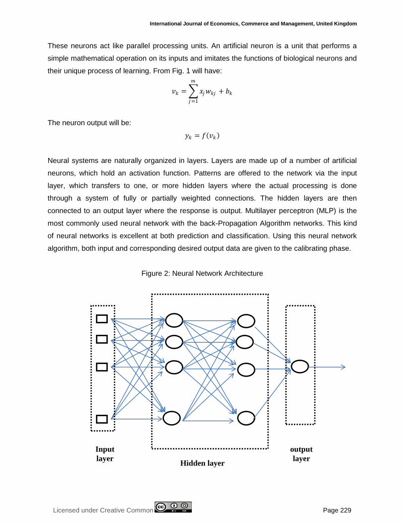
Neural systems are naturally organized in layers. Layers are made up of a number of artificial

neurons, which hold an activation function. Patterns are offered to the network via the input

layer, which transfers to one, or more hidden layers where the actual processing is done

through a system of fully or partially weighted connections. The hidden layers are then

connected to an output layer where the response is output. Multilayer perceptron (MLP) is the

most commonly used neural network with the back-Propagation Algorithm networks. This kind

of neural networks is excellent at both prediction and classification. Using this neural network

algorithm, both input and corresponding desired output data are given to the calibrating phase.

Figure 2: Neural Network Architecture

Input

layer

output

layer Hidden layer

http://ijecm.co.uk/

© Zaidi & Amirat


According to Wierenga and Kluytmans (1994) ANN can be proceeded in four steps:

Step 1

Set the number of input and output layers , the analyst must decide how many intermediate or

hidden layers, the network offers only limited possibilities of adaptation, with one hidden layer is

capable, with a sufficient number of neurons to approximate all continuous function ( Hornik,

1991). A second hidden layer takes into account the discontinuities or detects relationships and

interactions between variables. Indeed, in our study the use of hidden layers is very useful to

detect all non-linear relationships between variables in the model. After several

experimentations we used four (4) layers.

Step 2

Determine the number of neurons in layers. Each additional neuron allows taking into account

specific profiles of input neurons. A more large number therefore allows better match the data

presented but decreases capacity generalization of the network. Here again no general rule but

empirical rules. The size of the hidden layer must be either equal to that of the input layer

(Wierenga and Kluytmans , 1994) or is equal to 75% of the latter (Venugopal Baet, 1994) or is

equal to the square root of the number of neurons in the input and output layer (Shepard,1990).

In our study we chose the approach of setting a maximum number of nodes in each

hidden layer. Then, we eliminated those have no utility for the learning procedure. So the

number of input nodes is equal to number of independent variables which is 5 (higher price,

lower price, open price, oil and turnover). And the number of output nodes is equal to number of

dependent variables which is 1 (index returns).

Figure 3: ANN structure



Step 3

Select the transfer function .because of the dependent variable is bounded [0,1], the logistic

function is chosen for both hidden layers to the output layer(tansig)

Figure 4: Tan – sigmoid Transfer Function

Step 4

Choose learning. The retro-propagation algorithm requires determination of the adjustment

parameter of the synaptic weight in each iteration. We have retained the learning method

(trainrp) which is a network training function that updates weight and bias values according to

the resilient back propagation algorithm (RPROP).

The assessment of the prediction performance of the different soft computing models

was done with matlab 2013 by quantifying the prediction obtained on an independent data set.

The mean absolute error (MAE) was used to study the performance of the trained forecasting

models for the testing years. MAE is defined as follows:

𝑀𝐴𝐸 =1

𝑁 𝑃𝑝𝑟𝑒𝑑𝑖𝑐𝑡𝑒𝑑 𝑖 − 𝑃𝑎𝑐𝑡𝑢𝑎𝑙 𝑖

𝑁

𝑖=1

Where:

𝑃𝑝𝑟𝑒𝑑𝑖𝑐𝑡𝑒𝑑 𝑖 is the predicted return on day i

𝑃𝑎𝑐𝑡𝑢𝑎𝑙 𝑖 is actual return on day i

N is the number of observations

We used also Mean square error is used for evaluating the prediction accuracy of the model:

𝑀𝑆𝐸 =1

𝑁 𝑃𝑝𝑟𝑒𝑑𝑖𝑐𝑡𝑒𝑑 𝑖 − 𝑃𝑎𝑐𝑡𝑢𝑎𝑙 𝑖

2𝑁

𝑖=1

http://ijecm.co.uk/

© Zaidi & Amirat


Table 9: ANN Structure

Neural network MLP Transfer function Tan-sigmoid

Number of hidden layer 4 Iterations 70

Number of nodes in input layer 5 Training pattern 1342

Number of nodes in hidden layer 1 8 Test pattern 336

Number of nodes in hidden layer 2 8 MAE (Training) 0.2352

Number of nodes in hidden layer 3 5 MSE (Training) 0.1183

Number of nodes in hidden layer 4 3 MAE (Prediction) 0.2660

Number of nodes in output layer 1 MSE (Prediction) 0.1368

The network is trained by repeatedly presenting it with both the training and test data sets. To

identify when to stop training, two parameters, namely the MAE and MSE of both the training

and test sets were used. After 70 iterations, the MAE and MSE of the training set was 0.2352

and 0.1183 respectively, while those of test set was 0.2660 and 0.1368. The training was

stopped after 70 iterations as there was no significant decrease in both parameters. Thus, any

further training was not going to be productive or cause any significant changes. The prediction

accuracy of the training data is 84.12% and that of test data is 81.84%.

From the result shown in Table 9, it is observed that the predicted values are in good agreement

with exact values and the predicted error is very less. Also the results obtained clearly

demonstrate that MLP method is reliable and accurate and effective for forecasting stock

returns. Therefore the proposed ANN model with the developed structure shown in Table 9 can

perform good prediction in stock market.

Figure 5: Mean Squared Errors

0 5 10 15 20 25 30

10-2

10-1

100

Best Validation Performance is 0.091867 at epoch 26

Me

an

Sq

ua

red

Err

or

(m

se

)

32 Epochs

Train

Validation

Test

Best



CONCLUSION

In this paper, an attempt is made to explore the use of logistic regression to determine the

factors which significantly affect the evolution of the stock index. Logistic regression method

helps the investor to form an opinion about the time to invest. It may be observed that four

variables i.e. open price, higher price, lower price and oilcan classify up to 81.55% into two

categories up and down. This prediction rate is very good, so it can be used for prediction with

higher accuracy.

This study has also employed neural network to predict the direction of stock index

return. Multi-layer perceptron network is trained using Tan-sigmoidal algorithm. The prediction

accuracy of the model is high both for the training data (84.12%) and test data (81.84%).

We can deduce from this study that the use of logistic regression and neural network

give us very close result. But, both methods give us a good result of prediction with very high

accuracy using a mixture of fundamental and technical variables. So this study must be

extended to use these methods in the prediction and classification of stock returns.

REFERENCES

Altman, E., M.Giancarlo, and F.Varentto (1994), .Corporate Distress Diagnosis: Comparisons using Linear Discriminant Analysis and Neural Networks (the Italian Experience), Journal of Banking and Finance, Vol.18, pp.505-29.

Bajestani, N. S. and A. Zare (2011). "Forecasting TAIEX using improved type 2 fuzzy time series." Expert Systems with Applications 38(5): 5816-5821.

Boyacioglu, M. A. and D. Avci (2010). "An Adaptive Network-Based Fuzzy Inference System (ANFIS) for the prediction of stock market return: The case of the Istanbul Stock Exchange." Expert Systems with Applications 37(12): 7908-7912.

Chih-Fong, T. and H. Yu-Chieh (2010). "Combining multiple feature selection methods for stock prediction: Union, intersection, and multi-intersection approaches."Decis. Support Syst. 50(1): 258-269.

Collins, E., Ghosh, S. and Svofield. C. (1998), .An Application of a multiple Neural Network Learning System to Emulation of Mortgage Underwriting Judgements., Proceedings of the IEEE International Conference on Neural Networks, Vol.2,pp.459-466.

Dutta, A. et al. (2008).”Classification and Prediction of Stock Performance using Logistic Regression: An Empirical Examination from Indian Stock Market: Redefining Business Horizons”: McMillan Advanced Research Series.p.46-62.

Dutta, S., and Shekhar, S. (1998), .Bond Rating: A Non-conservative Application of Neural Networks., Proceedings of the IEEE International Conference on Neural networks, Vol.2, pp.443-450.

Esfahanipour, A. and W. Aghamiri (2010). "Adapted Neuro- Fuzzy Inference System on indirect approach TSK fuzzy rule base for stock market analysis." Expert Systems with Applications 37(7): 4742-4748.

Hadavandi, E., H. Shavandi, et al. (2010). "Integration of genetic fuzzy systems and artificial neural networks for stock price forecasting." Knowledge-Based Systems 23(8): 800-808.

Haines, L. M. et.al. (2007).”D-optimal Designs for Logistic Regression in Two Variables, mODa 8-Advances in Model-Oriented Designed and Anaysis” : Physica-Verlag HD. p.91-98.

http://ijecm.co.uk/

© Zaidi & Amirat


Hair,Black, Babin,Anderson, Tatham (2008) “Multivariate Data Analysis” Sixth edition Pearson Education, Inc.

Hatfield, Gay B., and White, A. Jay (1996), .Bond Rating Changes: Neural Net Estimates for Bank Holding Companies., Working Paper.

Huang, Q. Cai, Y., Peng, J. (2007) .”Modeling the Spatial Pattern of Farmland Using GIS and Multiple Logistic Regression: A Case Study of Maotiao River Basin,” Guizhou Province, China. Environmental Modeling and Assessment, 12(1):55-61.

Hutchinson, James M. Andrew W.Lo and Tomaso Poggio (1994), .A Non-Parametric Approach to Pricing and Hedging Derivatives Securities Via Learning Networks. . The Journal of Finance, Vol.XLIX, No.3, July.

Kara, Y., M. AcarBoyacioglu, et al. (2010). "Predicting direction of stock price index movement using artificial neural networks and support vector machines: The sample of the Istanbul Stock Exchange." Expert Systems with Applications In Press, Corrected Proof.

Kusturelis, Jason E. (1998) .Forecasting Financial Markets using Neural Networks: An Analysis of Methods and Accuracy., Master of Science in Management Thesis, Department of System Management, http://www.nps.navy.mil/Code36/ KUTSURE.html

Lean Yu, Huanhuan Chen, et al. (2009). "Evolving Least Squares Support Vector Machines for Stock Market Trend Mining." IEEE TRANSACTIONS ON EVOLUTIONARY COMPUTATION VOL. 13(NO. 1).

Lee, S. (2004). “Application of Likelihood Ratio and Logistic Regression Models to Landslide Susceptibility Mapping Using GIS”. Environmental Management.34(2):223-232.

Lee, S. ,Ryu ,J.Kim, L. (2007). “Landslide Susceptibility Analysis and Its Verification Using Likelihood Ratio, Logistic Regression, and Artificial Neural Network Models: Case Study of Youngin, Korea”. Landslides. 4: 327–338.

McCluskey, Peter C. (1993) .Feed-forward and Recurrent Neural Networks and Genetic Programs for Stock Market and Time Series Forecasting., Department of Computer Science, Brown University, September.

Ni, L.-P., Z.-W. Ni, et al. (2011). "Stock trend prediction based on fractal feature selection and support vector machine." Expert Systems with Applications 38(5): 5569- 5576.

Ohlson, J. (1980). “Financial ratios and the probabilistic prediction of bankruptcy”. Journal of Accounting Research, 18:109-31.

Pardo,J.A., Pardo L, Pardo, M.C (2005) “Minimum Ө-divergence Estimator in logistic regression Models”, Statistical Papers, No 47, 91-108.

Refenes , A.N., Bentz, Y. Bunn, D.W., Burgess, A.N. and Zapranis, A.D. (1997) .Financial Time Series Modeling with Discounted Least Squares back Propagation., Neuro Computing Vol. 14, pp.123-138.

Shen, W., X. Guo, et al. (2010). "Forecasting stock indices using radial basis function neural networks optimized by artificial fish swarm algorithm

Suan, Tan Sen and KohHianChye (1997), .Neural Network Applications in Accounting and Business., Accounting and Business Review, Vol.4, No.2, July, pp.297-317.

tsalakis, G. S. and K. P. Valavanis (2009). "Surveying stock market forecasting techniques - Part II: Soft computing methods." Expert Systems with Applications 36(3, Part 2): 5932-5941.

Zavgren, C. 1985. Assessing the vulnerability to failure of American industrial firms: A logistic analysis, Journal of Business Finance and Accounting 12(1):19–45.

Zmijewski, M.E .1984. Methodological issues related to the estimation of financial distress prediction models, Journal of Accounting Research 22:59-82.

forecasting stock market trends by …ijecm.co.uk/wp-content/uploads/2016/06/4614.pdf ·...

Documents