forecasting risk using auto regressive integrated …...tive role in market efficiency for price...

RESEARCH Open Access

Forecasting risk using auto regressiveintegrated moving average approach: anevidence from S&P BSE SensexMadhavi Latha Challa1* , Venkataramanaiah Malepati2 and Siva Nageswara Rao Kolusu 1

* Correspondence: [email protected] of Management Studies,Vignan’s Foundation for Science,Technology & Research, Guntur,Andhra Pradesh, IndiaFull list of author information isavailable at the end of the article

Abstract

The primary objective of the paper is to forecast the beta values of companies listed onSensex, Bombay Stock Exchange (BSE). The BSE Sensex constitutes 30 top mostcompanies listed which are popularly known as blue-chip companies. To reach out thepredefined objectives of the research, Auto Regressive Integrated Moving Averagemethod is used to forecast the future risk and returns for 10 years of historical datafrom April 2007 to March 2017. Validation accomplished by comparison of forecastedand actual beta values for the hold back period of 2 years. Root-Mean-Square-Error andMean-Absolute-Error both are used for accuracy measurement. The results revealedthat out of 30 listed companies in the BSE Sensex, 10 companies’ exhibits high betavalues, 12 companies are with moderate and 8 companies are with low beta values.Further, it is to note that Housing Development Finance Corporation (HDFC) exhibitsmore inconsistency in terms of beta values though the average beta value is lowestamong the companies under the study. A mixed trend is found in forecasted betavalues of the BSE Sensex. In this analysis, all the p-values are less than the F-stat valuesexcept the case of Tata Steel and Wipro. Therefore, the null hypotheses were rejectedleaving Tata Steel and Wipro. The values of actual and forecasted values are showingthe almost same results with low error percentage. Therefore, it is concluded from thestudy that the estimation ARIMA could be acceptable, and forecasted beta values areaccurate. So far, there are many studies on ARIMA model to forecast the returns of thestocks based on their historical data. But, hardly there are very few studies whichattempt to forecast the returns on the basis of their beta values. Certainly, the attemptso made is a novel approach which has linked risk directly with return. On the basis ofthe present study, authors try to through light on investment decisions by linking itwith beta values of respective stocks. Further, the outcomes of the present studyundoubtedly useful to academicians, researchers, and policy makers in their respectivearea of studies.

Keywords: Akaike Information Criteria (AIC), Bombay Stock Exchange (BSE), AutoRegressive Integrated Moving Average (ARIMA), Beta, Time series

JEL classification: G12, G14, G17

Financial Innovation

© The Author(s). 2018 Open Access This article is distributed under the terms of the Creative Commons Attribution 4.0 InternationalLicense (http://creativecommons.org/licenses/by/4.0/), which permits unrestricted use, distribution, and reproduction in any medium,provided you give appropriate credit to the original author(s) and the source, provide a link to the Creative Commons license, andindicate if changes were made.

Challa et al. Financial Innovation (2018) 4:24 https://doi.org/10.1186/s40854-018-0107-z

http://crossmark.crossref.org/dialog/?doi=10.1186/s40854-018-0107-z&domain=pdf

http://orcid.org/0000-0003-0861-9513

mailto:[email protected]

mailto:[email protected]

http://creativecommons.org/licenses/by/4.0/

IntroductionThe investments in stock market would produce profits as well as losses. But investors

want to maximize their profits instead of losses by analyzing stock market conditions.

This can be achievable when the risk is predictable in scientific manner. Risk aversion

is one of the interesting and important discussions among cult of investors, policy

makers, researchers, financial practitioners etc. The movements of returns and risks in

the stock market had noteworthy inferences on portfolio diversification and stock mar-

ket vulnerability. Both risks and returns are two sides of the coin and every successful

step undertaken by the investors could be turned into high returns which depend on

efficient and rational behavior of investors (Kaufman, G., 1995).

In 1986 the BSE Sensex was started. Gradually it has become the primary proxy for

the Bombay Stock Exchange (BSE) and considered as barometer of Indian economy.

The free float methodology has been used to calculate index level at any point of time

frame and it influences the market movement of 30 largest and actively traded stocks

or companies relative to base period. Every day Stock movements are changed because

of existence of volatility in market conditions. The BSE Sensex prices are goes up ward

direction, when the stocks of major companies on BSE prices gone up and vice versa.

Statement of the problem and research gap

In recent past, the performance of the stock markets is considered as barometer of

economy of a country. But, the appraisal of the performance of the stock market is not

so easy in given social, economical and political environment. The stock markets are

exhibiting more volatile across the world economies. These fluctuations in the prices of

stocks are very wide in developing economies where information asymmetry plays vital

role. India, as developing country, it is also not exceptional to the menace of unwanted

and excess volatility in the prices of stocks listed in its respective stock markets. Many

a times, Indian stock market has witnessed nightmare to millions of investors where

they had lost their lifetime savings in a day. In this juncture, the present inquiry con-

centrates on systematic risk and expected returns of stock in the time horizon because

these are uncertain and influences more in behavior of investor. Prediction of return to

the given risk associated with a particular security is a common phenomenon but pre-

diction of appropriate stock for investment merely on beta and testing their validity is

certainly a novel and it would contribute some addition to the existing literature.

Objectives of the study

The primary objective of the study is to test the validity of prediction of fruitful stocks

on the basis of their beta values with reference to BSE Sensex. Further, the following

are the specific objectives. These are: to

(i) Find the beta values of each stock listed on BSE Sensex and determine their degree

of risk on the basis of betas so found;

(ii) Compare and contrast each individual stock beta with portfolio’s (BSE Sensex) for

investment decision making; and

(iii)Validate the accuracy of forecasting risk with actual values over the holding period

(test period) of two years.

Challa et al. Financial Innovation (2018) 4:24 of 17

Literature reviewChan and Kwok (2017) examined the roles of risk-sharing and other factors in stock

price revaluation during liberalization period in connection to Shanghai Stock Ex-

change. They have found that risk-sharing was a significant mechanism in price revalu-

ation of stocks. Further, they found strong evidence that market imperfections hindered

the incorporation of firm-specific information into stock prices. Furthermore, they

added that market liquidity, information asymmetry, and insider trading played a nega-

tive role in market efficiency for price adjustment (Brunnermeier, M., Pedersen, L.,

2009, Moussa, A., 2011). Asset pricing theory predicts that an asset’s expected return is

positively associated with its exposure to systematic risk (De Bandt, O., Hartmann, P.,

2000, Hansen, L.P., 2013). However, empirical evidence supporting this prediction

has been mixed, as it is often found that systematic risk is not priced

cross-sectional (e.g., Fama and French, 2004). Chari and Henry (2004) note that

stock market liberalizations reduce systematic risk because the relevant source of

systematic risk becomes the world market; therefore, liberalizations represent an

exogenous change that enables us to test the prediction from theory (Chakrabarty,

K.C., (2012).

Jyothi et al. (2017) explains under the unconditional idiosyncratic volatility specifica-

tion, the firm size, cash flows to price ratio and market capitalizations are significant

factors. Moreover they found that size, Liquidity, momentum returns are the determi-

nants under the conditional idiosyncratic volatility. They support under diversified

portfolio and suggest based on empirical findings that firm specific fundamentals are

significant determinants of unsystematic risk.

The conventional portfolio theory of finance holds that rational investors in perfect

capital markets diversify unsystematic risk completely by holding uncorrelated assets in

their portfolio (Markowitz 1952), and early theoretical models hypothesize that system-

atic market risk is the sole determinant of expected stock returns (e.g., Sharpe 1964;

Lintner 1965; Black 1976).

Bianconi et al. (2017) examines the effect of information on the top ten financial in-

stitution’s tail risk and systematic risk by using the information of observed prices of

put and call options or newspaper articles. They use Garcia’s (2013) data as a measure

of CBOE (Chicago Broad of Exchange) volatility Index VIX and market sentiment. They

found that very little significant causality using dynamic feedback in terms of volatility.

Research design and methodologyTo reach out the predefined objectives of the study, the data of each company regis-

tered on BSE Sensex and the data of BSE Sensex (as a portfolio) from Bombay Stock

Exchange Ltd. has been collected for the period of 10 years. For this work, daily open

and close prices of stocks registered in BSE Sensex are used as a data. The collected

data of each company registered is planned to compare with BSE Sensex as a whole so

as to calculate beta values for each company.

BETA calculation

Beta is a measure to determine the stock market volatility in terms of portfolio or se-

curity fluctuations used in fundamental analysis. When evaluating risk, the stock price


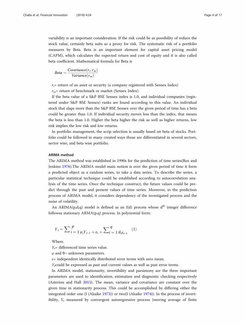
variability is an important consideration. If the risk could be as possibility of reduce the

stock value, certainly beta suits as a proxy for risk. The systematic risk of a portfolio

measures by Beta. Beta is an important element for capital asset pricing model

(CAPM), which calculates the expected return and cost of equity and it is also called

beta coefficient. Mathematical formula for Beta is

Beta ¼ Coveriance ri; rmð ÞVariance rmð Þ

ri= return of an asset or security (a company registered with Sensex Index)

rm= return of benchmark or market (Sensex Index)

If the beta value of a S&P BSE Sensex index is 1.0, and individual companies (regis-

tered under S&P BSE Sensex) ranks are found according to this value. An individual

stock that slaps more than the S&P BSE Sensex over the given period of time has a beta

could be greater than 1.0. If individual security moves less than the index, that means

the beta is less than 1.0. Higher the beta higher the risk as well as higher returns, low

risk implies the low risk and low returns.

In portfolio management, the scrip selection is usually based on beta of stocks. Port-

folio could be followed in many created ways those are differentiated in several sectors,

sector wise, and beta wise portfolio.

ARIMA method

The ARIMA method was established in 1990s for the prediction of time series(Box and

Jenkins 1976).The ARIMA model main notion is over the given period of time it form

a predicted object as a random series, to take a data series. To describe the series, a

particular statistical technique could be established according to autocorrelation ana-

lysis of the time series. Once the technique construct, the future values could be pre-

dict through the past and present values of time series. Moreover, in the prediction

process of ARIMA model, it considers dependency of the investigated process and the

noise of volatility.

An ARIMA(p,d,q) model is defined as an I(d) process whose dth integer difference

followsa stationary ARMA(p,q) process. In polynomial form:

Y t ¼X

i ¼ 1

p

φiY t−1 þ εt þX

i ¼ 1

q

θiεt−1ð1Þ

Where.

Yt= differenced time series value.

φ and θ= unknown parameters.

ε= independent identically distributed error terms with zero mean.

Ytcould be expressed as past and current values as well as past error terms.

In ARIMA model, stationarity, invertibility and parsimony are the three important

parameters are used to identification, estimation and diagnostic checking respectively

(Asteriou and Hall 2015). The mean, variance and covariance are constant over the

given time in stationarity process. This could be accomplished by differing either the

integrated order one (I (Akaike 1973)) or two(I (Akaike 1974)). In the process of invert-

ibility, Yt measured by convergent autoregressive process (moving average of finite


order). Box and Jenkins assumed that parsimony is a model, which produce well fore-

casting with extra coefficients and degree of freedom would be affected. This model is

better than an over parameterized model. In this study the ARIMA forecast for the

period of March 2017 to April 2019 was modeled by organizing the EViews software

which is applied for econometric analysis of time series.

Data

To reach out the predefined objectives of the study, as the study demands, researchers

used exclusively secondary data. The present investigation conducted using daily open

and close prices of BSE Sensex. The required data was collected from several resources

such as published and unpublished research, magazines, and official website of the BSE.

Table 1 Average year-wise beta values of companies listed in BSE Sensex during 2007–2017

Date 2008 2009 2010 2011 2012 2013 2014 2015 2016 2017 Average

Tata Motors DVR 0 4.78 0.48 0.73 1.25 1.48 1.05 1.75 1.4 1.41 1.43

ICICI Bank 1.08 1.45 1.29 1.32 1.32 1.58 1.46 1.46 1.36 1.62 1.39

Tata Steel 1.05 1.09 1.36 1.14 1.21 1.28 1.11 1.28 1.4 1.36 1.23

State Bank of India 1.14 1.08 1.03 0.87 1.15 1.42 1.18 1.31 1.3 1.56 1.20

Tata Motors 0.94 0.64 1.44 1.14 1.2 1.34 1.01 1.49 1.37 1.39 1.20

Axis Bank 0.53 1.46 1.1 1.08 1.23 1.34 1.46 1.39 1.13 1.24 1.20

Larsen & Toubro 1.14 1.08 1.26 0.84 1.2 1.48 1.37 1.29 1.16 1.12 1.19

Kotak Mahindra Bank 1.37 1.36 1.12 0.87 1.2 1.03 1.33 0.92 0.92 0.72 1.08

Adani Ports & SEZ 1.59 0.56 0.69 0.89 0.71 0.95 0.75 1.69 1.05 1.61 1.05

Reliance Industries 1.24 1.16 0.99 0.87 1.14 0.9 1.1 1.11 1.07 0.74 1.03

Mahindra & Mahindra 0.84 0.84 1.13 0.93 1.13 0.78 0.89 0.93 1.04 1.13 0.96

HDFC Bank 1.02 0.99 0.63 0.81 0.93 0.96 1.29 0.93 0.69 0.74 0.90

Oil and Natural Gas Corporation 0.39 0.54 0.7 0.5 0.7 1.09 1.16 1.31 1.16 0.62 0.82

Maruti Suzuki 0.75 0.66 0.6 0.54 0.73 0.69 0.71 1 0.81 1.17 0.77

BhartiAirtel 0.97 0.78 0.56 0.64 0.81 0.72 1.13 0.45 0.57 0.81 0.74

NTPC 1.04 0.68 0.54 0.38 0.74 0.68 0.69 1.07 0.69 0.86 0.74

ITC 0.48 0.59 0.84 0.53 0.55 0.73 0.9 0.62 0.91 0.94 0.71

Coal India 0.68 0.53 0.47 0.63 1.1 0.75 0.6 0.68

Power Grid Corporation of India 1.13 0.7 0.52 0.36 0.54 0.69 0.63 0.74 0.49 0.86 0.67

Tata Consultancy Services 0.67 0.95 0.62 0.74 0.87 0.57 0.62 0.49 0.55 0.45 0.65

Hero MotoCorp 0.6 0.3 0.58 0.55 0.53 0.53 0.74 0.72 0.82 1.01 0.64

Infosys 0.64 0.7 0.56 0.63 0.79 0.62 0.43 0.3 0.82 0.69 0.62

Cipla 0.34 0.41 0.5 0.44 0.49 0.57 0.44 0.66 0.9 0.51 0.53

Lupin 0.58 0.52 0.25 0.59 0.36 0.37 0.32 0.41 0.78 0.87 0.51

Sun Pharmaceutical 0.32 0.28 0.37 0.48 0.46 0.41 0.54 0.34 0.94 0.86 0.50

Wipro −0.14 0.63 0.92 0.67 0.73 0.54 0.34 0.38 0.48 0.43 0.50

Asian Paints 0.21 0.09 0.25 0.19 0.25 0.73 0.72 0.85 0.71 0.82 0.48

Hindustan Unilever 0.5 0.38 0.37 0.41 0.55 0.53 0.6 0.15 0.58 0.45 0.45

Dr. Reddy’s Laboratories 0.34 0.42 0.4 0.27 0.49 0.26 0.52 0.27 0.67 0.56 0.42

Housing Development FinanceCorporation

0.55 0.48 0.43 0.43 0.49 −0.79 0.6 0.49 0.72 −0.46 0.29

Source: Compiled by authors


The collected was processed and tabulated as per the needs of the study. It covers the

period of 10 years from April 2007 to March 2017.

Scope and limitations of the study

No study is exceptional to the completeness. The present study covers only BSE Sensex

leaving all the sectorial indices incorporated within otherwise these would have in-

cluded under the coverage of the study. Further, along the BSE, there other national

stock exchanges which are also considered as imperative stock exchanges in Indian

economy. But due to time, difficulty to arrive uniformity in some variables they were

ignored for the study.

Results and discussionThe following paragraphs are devoted to discuss the results arrived through the meth-

odology adopted for the purpose.

Table 1 exhibits average year-wise beta values of companies listed in BSE Sensex dur-

ing 2007–2017. It can be understand that those companies’ beta values which are hav-

ing more than one are more volatile in movement of prices of stocks; those who are

having less than one are less volatile. If the beta is near to one, the volatility of the

movement of the prices of the market equals to that of the movement of the prices of

individual company of portfolio/index. Usually, investors prefer less than 1 beta value

companies because these stocks are having less volatility, low risk and also lower

Fig. 1 Summary of average year-wise beta values of companies listed in BSE Sensex during 2008–17


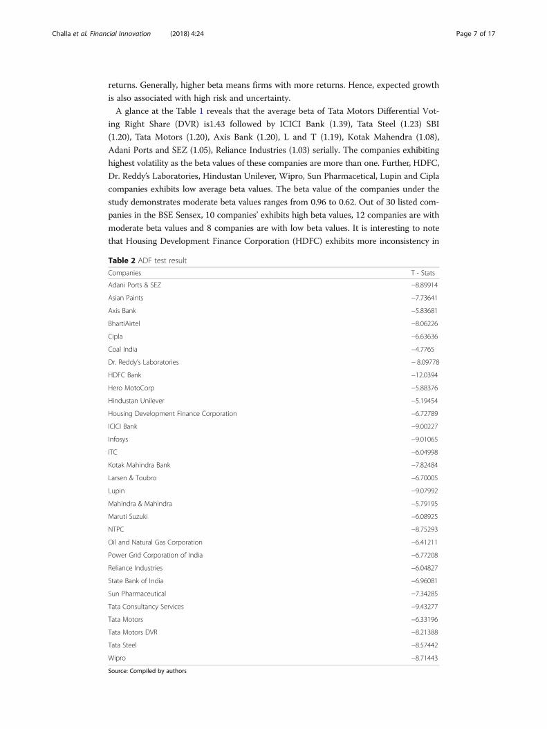
returns. Generally, higher beta means firms with more returns. Hence, expected growth

is also associated with high risk and uncertainty.

A glance at the Table 1 reveals that the average beta of Tata Motors Differential Vot-

ing Right Share (DVR) is1.43 followed by ICICI Bank (1.39), Tata Steel (1.23) SBI

(1.20), Tata Motors (1.20), Axis Bank (1.20), L and T (1.19), Kotak Mahendra (1.08),

Adani Ports and SEZ (1.05), Reliance Industries (1.03) serially. The companies exhibiting

highest volatility as the beta values of these companies are more than one. Further, HDFC,

Dr. Reddy’s Laboratories, Hindustan Unilever, Wipro, Sun Pharmacetical, Lupin and Cipla

companies exhibits low average beta values. The beta value of the companies under the

study demonstrates moderate beta values ranges from 0.96 to 0.62. Out of 30 listed com-

panies in the BSE Sensex, 10 companies’ exhibits high beta values, 12 companies are with

moderate beta values and 8 companies are with low beta values. It is interesting to note

that Housing Development Finance Corporation (HDFC) exhibits more inconsistency in

Table 2 ADF test result

Companies T - Stats

Adani Ports & SEZ −8.89914

Asian Paints −7.73641

Axis Bank −5.83681

BhartiAirtel −8.06226

Cipla −6.63636

Coal India −4.7765

Dr. Reddy’s Laboratories − 8.09778

HDFC Bank −12.0394

Hero MotoCorp −5.88376

Hindustan Unilever −5.19454

Housing Development Finance Corporation −6.72789

ICICI Bank −9.00227

Infosys −9.01065

ITC −6.04998

Kotak Mahindra Bank −7.82484

Larsen & Toubro −6.70005

Lupin −9.07992

Mahindra & Mahindra −5.79195

Maruti Suzuki −6.08925

NTPC −8.75293

Oil and Natural Gas Corporation −6.41211

Power Grid Corporation of India −6.77208

Reliance Industries −6.04827

State Bank of India −6.96081

Sun Pharmaceutical −7.34285

Tata Consultancy Services −9.43277

Tata Motors −6.33196

Tata Motors DVR −8.21388

Tata Steel −8.57442

Wipro −8.71443



terms of beta values though the average beta value is lowest among the companies under

the study. Furthermore, it can be observed that HDFC and Wipro are two companies

which exhibit negative beta values over the period of study (see Fig. 1).

The following paragraphs present the sequence of results i.e., Identification, Estima-

tion, Diagnostic check, Forecasting and Validation.

Identification

In this stage, the Augmented Dickie Fuller (ADF) test is used to ensure the level of data

series is stationary or not. The result of ADF test shows that the series has achieved a sta-

tionary state. The stationary could be identified according to the t-stats value. If the t-stats

Table 3 Akaike Information Criteria value (AIC)

Companies Selected ARMA model AIC value

Adani Ports & SEZ (Akaike 1974; Akaike 1979)(0,0) 2.419996205

Asian Paints (0,1)(0,2) 1.18300953

Axis Bank (Akaike 1974; Akaike 1976)(0,0) 1.412734755

BhartiAirtel (Akaike 1974; Akaike 1979)(0,0) 1.126284533

Cipla (0,2)(0,0) 1.036260176

Coal India (2,0)(0,0) 1.383862705

Dr. Reddy’s Laboratories (Akaike 1974)(0,0) 1.021199203

HDFC Bank (4,0)(0,0) 0.865074133

Hero MotoCorp (Akaike 1973; Akaike 1976)(0,0) 1.398471031

Hindustan Unilever (0,2) (Akaike 1973) 0.912515275

Housing Development FinanceCorporation

(0,0)(0,0) 3.890160664

ICICI Bank (0,2) (Akaike 1973; Akaike 1974) 0.576514289

Infosys (Akaike 1976) (Akaike 1973) 0.784789316

ITC (0,2)(0,0) 1.75706519

Kotak Mahindra Bank (Akaike 1973; Akaike 1974)(0,0) 1.126330283

Larsen & Toubro (Akaike 1974)(0,0) 1.669414571

Lupin (1,0)(0,0) 1.201107512

Mahindra & Mahindra (Akaike 1979)(0,0) 1.26508819

Maruti Suzuki (0,1)(0,0) 1.595029239

NTPC (Akaike 1974; Akaike 1976) (Akaike 1973; Akaike1974)

0.916387604

Oil and Natural Gas Corporation (0,1)(1,0) 2.473119679

Power Grid Corporation of India (1,0)(0,0) 1.028937003

Reliance Industries (Akaike 1974)(0,1) 0.472093637

State Bank of India (0,1)(0,0) 2.040875765

Sun Pharmaceutical (Akaike 1974; Akaike 1979)(1,0) 1.113411517

Tata Consultancy Services (Akaike 1974; Akaike 1976) (Akaike 1973) 1.105677727

Tata Motors (Akaike 1974; Akaike 1976) (Akaike 1973) 1.542142809

Tata Motors DVR (Akaike 1974; Akaike 1976)(0,2) 1.827594151

Tata Steel (Akaike 1974)(0,0) 1.449933246

Wipro (0,0)(1,0) 3.207891726



value is greater than the critical value (CV) at 5% level i.e. -2.888157, then it is considered

as stationary. In the present study, the calculated values of ADF test of all the companies

under the study are greater than that of critical values at 5% level of significance (Table 2).

Estimation

In this estimation stage, different ARIMA models are estimated using Akaike Informa-

tion Criteria (AIC) for comparison (Akaike 1981). AIC is used to determine the model

best fits a set of data series and it choose the best model to forecast the future data.

This is based upon the estimated log-likelihood of the model, number of observations

and number of parameters in the model. By using ARIMA models, the number of Auto

Regressive Moving Average (ARMA) terms could be determined. The maximum num-

ber of Auto Regressive (AR) or Moving Average (MA) coefficients has been specified to

determine the number of ARMA terms, then to estimate every model up to those max-

ima and then each model could be evaluated using its information criterion.

Fig. 2 Residual correlograms


After estimating each model along with calculated criterion, the model could be

chosen with the lowest criterion value. According to Stone (1981) and Lindley (1968),

the selection of best model represented by parsimony of parameters, it can take variety

of attributes of the chosen model. In this analysis, the estimated ARMA models are

225. The selected models along with AIC values are presented in Table 3.

Diagnostic check

The diagnostic check is essential check as it is used to check whether the residuals have

white noise characteristics or not. The Auto Correlation Function (ACF) and Partial

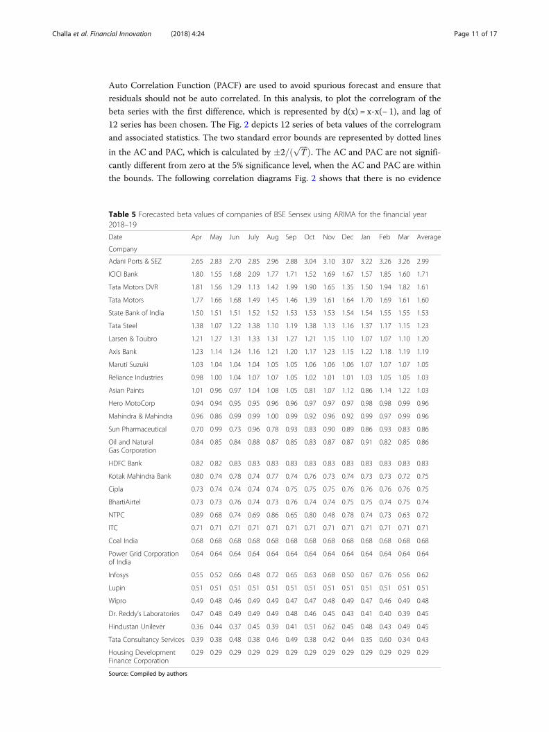
Table 4 Forecasted beta values of companies of BSE Sensex using ARIMA for the financial year2017–18

Date Apr May June July Aug Sep Oct Nov Dec Jan Feb Mar Average

Company

Adani Ports & SEZ 1.72 2.34 2.25 1.96 2.48 2.30 2.21 2.61 2.4 2.43 2.72 2.54 2.33

ICICI Bank 1.32 1.64 1.49 1.23 1.41 1.54 1.79 1.58 1.46 1.59 1.46 1.65 1.51

Tata Motors DVR 1.24 1.62 1.57 1.57 1.33 1.48 1.9 1.42 1.65 1.38 1.45 1.41 1.50

State Bank of India 1.45 1.46 1.46 1.47 1.47 1.48 1.48 1.48 1.49 1.49 1.50 1.50 1.48

Tata Motors 1.13 1.42 1.45 1.70 1.67 1.55 1.61 1.31 1.34 1.37 1.46 1.61 1.47

Tata Steel 1.26 0.99 1.40 1.30 1.00 1.35 1.34 1.02 1.30 1.36 1.04 1.26 1.22

Axis Bank 1.35 1.15 1.29 1.15 1.21 1.22 1.15 1.26 1.13 1.24 1.18 1.18 1.21

Larsen & Toubro 1.27 1.32 1.34 1.33 1.28 1.22 1.15 1.09 1.06 1.06 1.09 1.14 1.20

Maruti Suzuki 0.99 0.99 1.00 1.00 1.00 1.01 1.01 1.01 1.02 1.02 1.03 1.03 1.01

Reliance Industries 0.87 1.08 1.00 1.08 1.08 0.81 0.93 0.96 0.98 0.91 0.94 1.10 0.99

Mahindra & Mahindra 0.81 1.12 1.02 1.30 0.8 0.98 0.74 0.97 1.02 1.03 1.08 0.88 0.98

Asian Paints 0.94 0.82 0.97 1.07 1.04 0.99 0.65 0.80 0.95 0.77 0.97 1.04 0.92

Hero MotoCorp 0.61 0.62 1.00 0.99 0.99 0.88 0.88 0.89 0.93 0.94 0.94 0.93 0.88

Sun Pharmaceutical 0.72 1.05 0.52 1.03 0.53 1.10 0.60 1.10 0.65 1.02 0.62 1.05 0.83

NTPC 0.97 0.76 1.00 0.63 0.82 0.66 0.89 0.93 0.89 0.61 0.9 0.82 0.82

Kotak Mahindra Bank 1.12 0.58 1.02 0.64 0.95 0.68 0.89 0.71 0.86 0.73 0.83 0.74 0.81

HDFC Bank 0.82 0.67 0.88 0.70 0.81 0.77 0.82 0.79 0.82 0.81 0.82 0.81 0.79

ONGC 0.79 0.81 0.76 0.96 0.87 0.75 0.66 0.82 0.81 0.98 0.55 0.67 0.79

ITC 0.93 0.89 0.71 0.71 0.71 0.71 0.71 0.71 0.71 0.71 0.71 0.71 0.74

BhartiAirtel 0.71 0.39 0.96 0.75 0.55 0.89 0.72 0.67 0.81 0.74 0.7 0.79 0.72

Cipla 0.67 0.70 0.70 0.71 0.71 0.71 0.72 0.72 0.72 0.72 0.73 0.73 0.71

Coal India 0.66 0.61 0.67 0.67 0.68 0.68 0.68 0.68 0.68 0.68 0.68 0.68 0.67

Power Grid Corporation ofIndia

0.64 0.64 0.64 0.64 0.64 0.64 0.64 0.64 0.64 0.64 0.64 0.64 0.64

Infosys 0.44 0.55 0.61 0.44 0.78 0.6 0.71 0.64 0.49 0.7 0.76 0.60 0.61

Lupin 0.51 0.51 0.51 0.51 0.51 0.51 0.51 0.51 0.51 0.51 0.51 0.51 0.51

Wipro 0.52 0.47 0.36 0.54 0.54 0.43 0.45 0.45 0.53 0.44 0.39 0.53 0.47

Hindustan Unilever 0.21 0.39 0.31 0.45 0.36 0.39 0.54 0.73 0.46 0.5 0.42 0.52 0.44

Tata Consultancy Services 0.50 0.51 0.4 0.52 0.4 0.35 0.5 0.44 0.4 0.5 0.2 0.51 0.44

Dr. Reddy’s Laboratories 0.36 0.34 0.32 0.31 0.31 0.32 0.34 0.36 0.38 0.41 0.43 0.45 0.36

Housing DevelopmentFinance Corporation

0.29 0.29 0.29 0.29 0.29 0.29 0.29 0.29 0.29 0.29 0.29 0.29 0.29



Auto Correlation Function (PACF) are used to avoid spurious forecast and ensure that

residuals should not be auto correlated. In this analysis, to plot the correlogram of the

beta series with the first difference, which is represented by d(x) = x-x(− 1), and lag of

12 series has been chosen. The Fig. 2 depicts 12 series of beta values of the correlogram

and associated statistics. The two standard error bounds are represented by dotted lines

in the AC and PAC, which is calculated by �2=ð ffiffiffiffiT

p Þ. The AC and PAC are not signifi-

cantly different from zero at the 5% significance level, when the AC and PAC are within

the bounds. The following correlation diagrams Fig. 2 shows that there is no evidence

Table 5 Forecasted beta values of companies of BSE Sensex using ARIMA for the financial year2018–19

Date Apr May Jun July Aug Sep Oct Nov Dec Jan Feb Mar Average

Company

Adani Ports & SEZ 2.65 2.83 2.70 2.85 2.96 2.88 3.04 3.10 3.07 3.22 3.26 3.26 2.99

ICICI Bank 1.80 1.55 1.68 2.09 1.77 1.71 1.52 1.69 1.67 1.57 1.85 1.60 1.71

Tata Motors DVR 1.81 1.56 1.29 1.13 1.42 1.99 1.90 1.65 1.35 1.50 1.94 1.82 1.61

Tata Motors 1.77 1.66 1.68 1.49 1.45 1.46 1.39 1.61 1.64 1.70 1.69 1.61 1.60

State Bank of India 1.50 1.51 1.51 1.52 1.52 1.53 1.53 1.53 1.54 1.54 1.55 1.55 1.53

Tata Steel 1.38 1.07 1.22 1.38 1.10 1.19 1.38 1.13 1.16 1.37 1.17 1.15 1.23

Larsen & Toubro 1.21 1.27 1.31 1.33 1.31 1.27 1.21 1.15 1.10 1.07 1.07 1.10 1.20

Axis Bank 1.23 1.14 1.24 1.16 1.21 1.20 1.17 1.23 1.15 1.22 1.18 1.19 1.19

Maruti Suzuki 1.03 1.04 1.04 1.04 1.05 1.05 1.06 1.06 1.06 1.07 1.07 1.07 1.05

Reliance Industries 0.98 1.00 1.04 1.07 1.07 1.05 1.02 1.01 1.01 1.03 1.05 1.05 1.03

Asian Paints 1.01 0.96 0.97 1.04 1.08 1.05 0.81 1.07 1.12 0.86 1.14 1.22 1.03

Hero MotoCorp 0.94 0.94 0.95 0.95 0.96 0.96 0.97 0.97 0.97 0.98 0.98 0.99 0.96

Mahindra & Mahindra 0.96 0.86 0.99 0.99 1.00 0.99 0.92 0.96 0.92 0.99 0.97 0.99 0.96

Sun Pharmaceutical 0.70 0.99 0.73 0.96 0.78 0.93 0.83 0.90 0.89 0.86 0.93 0.83 0.86

Oil and NaturalGas Corporation

0.84 0.85 0.84 0.88 0.87 0.85 0.83 0.87 0.87 0.91 0.82 0.85 0.86

HDFC Bank 0.82 0.82 0.83 0.83 0.83 0.83 0.83 0.83 0.83 0.83 0.83 0.83 0.83

Kotak Mahindra Bank 0.80 0.74 0.78 0.74 0.77 0.74 0.76 0.73 0.74 0.73 0.73 0.72 0.75

Cipla 0.73 0.74 0.74 0.74 0.74 0.75 0.75 0.75 0.76 0.76 0.76 0.76 0.75

BhartiAirtel 0.73 0.73 0.76 0.74 0.73 0.76 0.74 0.74 0.75 0.75 0.74 0.75 0.74

NTPC 0.89 0.68 0.74 0.69 0.86 0.65 0.80 0.48 0.78 0.74 0.73 0.63 0.72

ITC 0.71 0.71 0.71 0.71 0.71 0.71 0.71 0.71 0.71 0.71 0.71 0.71 0.71

Coal India 0.68 0.68 0.68 0.68 0.68 0.68 0.68 0.68 0.68 0.68 0.68 0.68 0.68

Power Grid Corporationof India

0.64 0.64 0.64 0.64 0.64 0.64 0.64 0.64 0.64 0.64 0.64 0.64 0.64

Infosys 0.55 0.52 0.66 0.48 0.72 0.65 0.63 0.68 0.50 0.67 0.76 0.56 0.62

Lupin 0.51 0.51 0.51 0.51 0.51 0.51 0.51 0.51 0.51 0.51 0.51 0.51 0.51

Wipro 0.49 0.48 0.46 0.49 0.49 0.47 0.47 0.48 0.49 0.47 0.46 0.49 0.48

Dr. Reddy’s Laboratories 0.47 0.48 0.49 0.49 0.49 0.48 0.46 0.45 0.43 0.41 0.40 0.39 0.45

Hindustan Unilever 0.36 0.44 0.37 0.45 0.39 0.41 0.51 0.62 0.45 0.48 0.43 0.49 0.45

Tata Consultancy Services 0.39 0.38 0.48 0.38 0.46 0.49 0.38 0.42 0.44 0.35 0.60 0.34 0.43


0.29 0.29 0.29 0.29 0.29 0.29 0.29 0.29 0.29 0.29 0.29 0.29 0.29



and signs of standard error and all of the spikes were within the standard error bars as

shown in Fig. 2.

Forecasting

The forecasting stage is used to find the future beta values for a single series based

upon an ARIMA model using the automatic ARIMA forecasting method by E-views

software. It allows the user to determine the appropriate specification of ARIMA. It is

also useful to forecast the future data series. Forecasted values of companies of BSE

Sensex using ARIMA for the period of study are portrayed in Table 4.

It can be observed from the Table 1 that the beta values of companies under study ex-

hibits incremental growth in their respective beta values leaving few companies when we

compare the beta values between April 2017 and March 2018. Axis Bank, L and T, NTPC,

Kotak Mahindra Bank, HDFC Bank, ITC and Cola India companies under the study are

exhibited a reverse trend with decline of beta values between April 2017 and March 2018.

A very few companies did not shown any major movements during the forecasted period.

Forecasted beta values of companies under the study are shown in Table 5. A glance

at the table reveals there is a mixed trend in the growth/decline of beta values of com-

panies under the study for the reference period. The average beta value is highest in

Adani Ports and SEZ (2.99) while the lowest is recorded in HDFC (0.29).

Tables 4 and 5 represent the forecasted beta values to estimate the risk in the future. From

the Tables 4 and 5 authors analyze three categories of investment risks. These are defensive,

moderate and aggressive betas. Based on these three kinds of risks, investors can choose the

company that they would like to invest on the basis of their risk bearing capacity. If the beta

is greater than one then the risk is more as well as returns too. If the beta is near to one or

equal to one, then it is said to be that the volatility or fluctuations of the company equals to

the market. If the beta value is less than one it attributes less risk with less returns.

Historical and forecasted beta values of companies under the study for the reference

period after applying the ARIMA process are exhibited in Fig. 3.

Fig. 3 Historical and forecasted beta values of companies listed in BSE Sensex using ARIMA


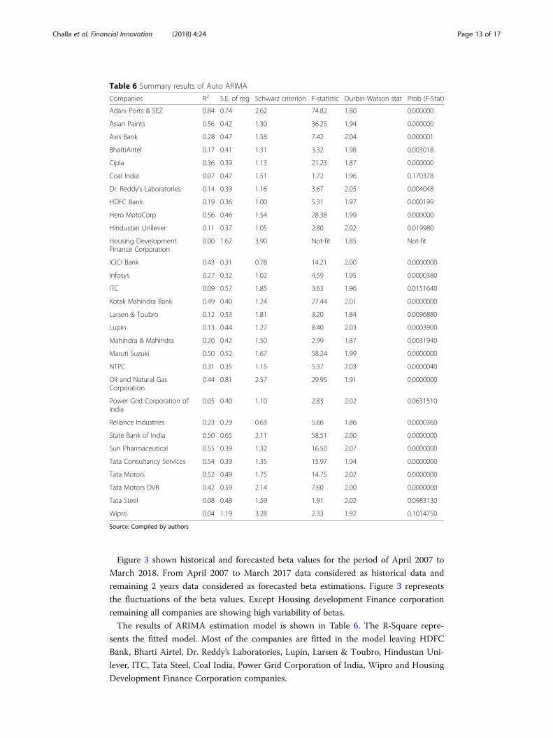
Figure 3 shown historical and forecasted beta values for the period of April 2007 to

March 2018. From April 2007 to March 2017 data considered as historical data and

remaining 2 years data considered as forecasted beta estimations. Figure 3 represents

the fluctuations of the beta values. Except Housing development Finance corporation

remaining all companies are showing high variability of betas.

The results of ARIMA estimation model is shown in Table 6. The R-Square repre-

sents the fitted model. Most of the companies are fitted in the model leaving HDFC

Bank, Bharti Airtel, Dr. Reddy’s Laboratories, Lupin, Larsen & Toubro, Hindustan Uni-

lever, ITC, Tata Steel, Coal India, Power Grid Corporation of India, Wipro and Housing

Development Finance Corporation companies.

Table 6 Summary results of Auto ARIMA

Companies R2 S.E. of reg Schwarz criterion F-statistic Durbin-Watson stat Prob (F-Stat)

Adani Ports & SEZ 0.84 0.74 2.62 74.82 1.80 0.000000

Asian Paints 0.56 0.42 1.30 36.25 1.94 0.000000

Axis Bank 0.28 0.47 1.58 7.42 2.04 0.000001

BhartiAirtel 0.17 0.41 1.31 3.32 1.98 0.003018

Cipla 0.36 0.39 1.13 21.23 1.87 0.000000

Coal India 0.07 0.47 1.51 1.72 1.96 0.170378

Dr. Reddy’s Laboratories 0.14 0.39 1.16 3.67 2.05 0.004048

HDFC Bank 0.19 0.36 1.00 5.31 1.97 0.000199

Hero MotoCorp 0.56 0.46 1.54 28.38 1.99 0.000000

Hindustan Unilever 0.11 0.37 1.05 2.80 2.02 0.019980


0.00 1.67 3.90 Not-fit 1.85 Not-fit

ICICI Bank 0.43 0.31 0.78 14.21 2.00 0.0000000

Infosys 0.27 0.32 1.02 4.59 1.95 0.0000380

ITC 0.09 0.57 1.85 3.63 1.96 0.0151640

Kotak Mahindra Bank 0.49 0.40 1.24 27.44 2.01 0.0000000

Larsen & Toubro 0.12 0.53 1.81 3.20 1.84 0.0096880

Lupin 0.13 0.44 1.27 8.40 2.03 0.0003900

Mahindra & Mahindra 0.20 0.42 1.50 2.99 1.87 0.0031940

Maruti Suzuki 0.50 0.52 1.67 58.24 1.99 0.0000000

NTPC 0.31 0.35 1.15 5.37 2.03 0.0000040

Oil and Natural GasCorporation

0.44 0.81 2.57 29.95 1.91 0.0000000

Power Grid Corporation ofIndia

0.05 0.40 1.10 2.83 2.02 0.0631510

Reliance Industries 0.23 0.29 0.63 5.66 1.86 0.0000360

State Bank of India 0.50 0.65 2.11 58.51 2.00 0.0000000

Sun Pharmaceutical 0.55 0.39 1.32 16.50 2.07 0.0000000

Tata Consultancy Services 0.54 0.39 1.35 15.97 1.94 0.0000000

Tata Motors 0.52 0.49 1.75 14.75 2.02 0.0000000

Tata Motors DVR 0.42 0.59 2.14 7.60 2.00 0.0000000

Tata Steel 0.08 0.48 1.59 1.91 2.02 0.0983130

Wipro 0.04 1.19 3.28 2.33 1.92 0.1014750



Forecasting

These companies are having less than 20% of R-Square. Standard Error Regression (S.E

of Reg) represents how wrong the regression model. The smaller values of S.E of Reg.

indicate that observations are closer to the fitted line. The alternative way of AIC is

Schwarz Criterion (SC) (Schwarcz, S.L., 2008), it imposes a larger penalty for additional

coefficients (Akaike 1987). Durbin –Watson (DW) statistic is used to measure the serial

correlation of the residuals. The evidence of positive serial correlation could be exited

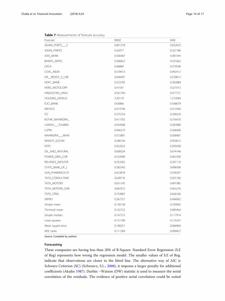
Table 7 Measurements of forecast accuracy

Forecast RMSE MAE

ADANI_PORTS___S 0.841378 0.652633

ASIAN_PAINTS 0.42077 0.321786

AXIS_BANK 0.500367 0.387344

BHARTI_AIRTEL 0.506822 0.431662

CIPLA 0.46884 0.379596

COAL_INDIA 0.578413 0.492412

DR__REDDY_S_LAB 0.646997 0.539812

HDFC_BANK 0.322295 0.282889

HERO_MOTOCORP 0.41597 0.321013

HINDUSTAN_UNILE 0.561764 0.477721

HOUSING_DEVELO 3.30179 1.272049

ICICI_BANK 0.63866 0.548679

INFOSYS 0.414746 0.312569

ITC 0.375254 0.290329

KOTAK_MAHINDRA_ 0.417355 0.316470

LARSEN___TOUBRO 0.354568 0.287889

LUPIN 0.446219 0.346406

MAHINDRA___MAHI 0.372881 0.308901

MARUTI_SUZUKI 0.580104 0.450615

NTPC 0.452623 0.395638

OIL_AND_NATURAL 0.608324 0.474146

POWER_GRID_COR 0.533949 0.461928

RELIANCE_INDUSTR 0.353265 0.281110

STATE_BANK_OF_I 0.582342 0.498306

SUN_PHARMACEUTI 0.423818 0.334507

TATA_CONSULTANC 0.638716 0.501766

TATA_MOTORS 0.631745 0.491985

TATA_MOTORS_DVR 0.687075 0.565276

TATA_STEEL 0.733887 0.626166

WIPRO 0.567257 0.494062

Simple mean 0.130158 0.100902

Trimmed mean 0.102722 0.085454

Simple median 0.147315 0.117914

Least-squares 0.151789 0.116337

Mean square error 0.108251 0.084964

MSE ranks 0.111369 0.090427



when the value of DW is less than 2. In the present study almost all companies DW is

very close to 2, this value indicates the presence of positive serial correlation in the re-

siduals. F-Statistic represents the regression output from the hypothesis test that all of

the slope coefficients are zero. The p-value denoted as prob. (F-Stat), which specifies

the marginal significance level of F-test. The null hypothesis could be rejected when

the p-value is less than the significance level i.e. 0.05, which shows that all slope coeffi-

cients are equal to zero. In this analysis, all the p-values are less than the F-stat values.

Therefore, the null hypothesis could be rejected. The p-value is not significant in the

case of Tata Steel and Wipro, remaining all companies are having 5% significance level.

Validation

To measure the forecast of accuracy, authors run Forecast Evaluation model using

E-views software for the sample period of April 2012 to March 2015, and evalu-

ation sample period of April 2015 to March 2017. From the analysis, the accuracy

Fig. 4 Forecasted beta values of companies listed in BSE Sensex using Auto ARIMA

Table 8 Top 5 ranked companies in 3 divisions

Moderate companies Rank Aggressive companies Rank Defensive companies Rank

Housing Development Finance Corporation 1 State Bank of India 1 Hero MotoCorp 1

Dr. Reddy’s Laboratories 2 Tata Motors 2 Mahindra & Mahindra 2

Tata Consultancy Services 3 Tata Motors DVR 3 Asian Paints 3

Hindustan Unilever 4 ICICI Bank 4 Reliance Industries 4

Wipro 5 Adani Ports & SEZ 5 Maruti Suzuki 5



of the forecasting could be found for the validation purpose. To confirm the qual-

ity of accuracy Root Mean Square Error (RMSE) and Mean Absolute Error (MAE)

were calculated based on errors between forecasted and actual data, which is pre-

sented in Table 7.

Table 7 shows the results of validation or test results between the forecasted and ac-

tual values. The MAE is always less than the RMSE values in all the cases of registered

companies in BSE Sensex, which indicates that the error percentage is very less and the

values of actual and forecast showing the almost same results. Therefore, the estima-

tion ARIMA could be acceptable, and forecasted beta values are accurate.

FindingsFrom the analysis, authors have found the future beta values for the period of April

2017 to March 2019. From the Fig. 4 three categories of betas has been found. First

one is moderate beta, which indicates the same instability as compared with Sensex

and it equals to one. Second category is aggressive beta, which shows more instability

when compared to Sensex and it express the beta greater than one.

Last one is defensive beta; it represents the less instability with Sensex comparison

and it is less than one. According to the category the companies also segregated for the

convenience of investors.

Lower rank represents the less risk and higher vice versa. Higher risk taking investors

might get good returns in the future. Table 8 shows the less risky companies under

three divisions (Moderate, Aggressive, Defensive) of companies. The investors can take

investment decisions according to their choice.

ConclusionForecasting with Auto ARIMA provides a prediction based on historical data, in which

data has been applied by first order difference to remove white noise problems. In this

analysis Auto ARIMA estimated AIC values, which yielded the more accurate forecast

over the ten years period. In validation, the forecasted values are compared with actual

values over the hold back period of two years. From this analysis the more uncertainty

has been found when the forecast period is long term period, less uncertainty exists in

the case of short term period. From the analysis the different investors can choose

companies according to their risk aversion.

AbbreviationsACF: Auto Correlation Function; ADF: Augmented Dickie Fuller; AIC: Akaike Information Criteria; AR: Auto Regressive;ARIMA: Auto Regressive Integrated Moving Average; ARMA: Auto Regressive Moving Average; BSE: Bombay StockExchange; DW: Durbin –Watson; MA: Moving Average; MAE: Mean Absolute Error; PACF: Partial Auto CorrelationFunction; RMSE: Root Mean Square Error; S.E of Reg: Standard Error Regression; SC: Schwarz Criterion; Tata MotorsDVR: Tata Motors Differential Voting Right Share

Availability of data and materialsSource of Data sets are available in http://www.bseindia.com and http://finance.yahoo.com. Analyzed data uploadedas supplementary material files.

Authors’ contributionsStudy of conception and design: MLC, VM, SNRK. Acquisition of data: MLC. Analysis and interpretation of data: MLC.Supervision: VM, SNRK. Drafting of manuscript: MLC. Critical revision: VM, SNRK. All authors read and approved the finalmanuscript.

Authors’ informationCH. Madhavi Latha received her MBA degree in Finance from Jesus PG College, affiliated by JNTUH, Hyderabad,Telangana, India. She is pursuing Ph.D at Vignan’s Foundation for Science, Technology & Research, Guntur, Andhra


http://www.bseindia.com

http://finance.yahoo.com

Pradesh, India. She is also working as Assistant Professor in University of Gondar, Gondar, Ethiopia. She has more than5 publications in various international Journals / Conferences. Her research areas include Capital Asset Pricing,Dynamic changes in Stock market and Stock holders Interest.Dr. Venkataramanaiah Malepati obtained his M.Com., M.Phil., and PhD from Sri Venkateswara University, Tirupati andMBA from Pondicherry University. At present, he is Professor of Management, Department of Management Studies atGolden Valley Instigated Campus, Madanapally. So far, he has published 34 research papers/articles in reputed/referrednational/ international journals. Almost, the same number of papers/research articles has been presented in differentnational and international conferences/seminars. At present five books on his credit.Dr. K. Siva Nageswara Rao is working as an Assistant Professor of School of Management Studies at Vignan Foundationfor Science, Technology & Research, Guntur, Andhra Pradesh, India. He received his MBA degree in Finance fromAcharya Nagarjuna University, Andhra Pradesh, India and M.Phil Degree in Finance from MS University, Tiruelveli,Tamilnadu. He received his Ph.D degree from Acharya Nagarjuna University Guntur, Andhra Pradesh, India. He has15 years of teaching experience. He has more than 20 publications in various National and International Journals/Conferences. His main research interest includes Finance and Entrepreneurship.

Competing interestsAuthors declare that they have no competing interests.

Publisher’s NoteSpringer Nature remains neutral with regard to jurisdictional claims in published maps and institutional affiliations.

Author details1School of Management Studies, Vignan’s Foundation for Science, Technology & Research, Guntur, Andhra Pradesh,India. 2Institute of Management Studies, Golden Valley Integrated Campus (GVIC), Madanapalli, Chittoor 517 325, India.

Received: 1 February 2018 Accepted: 1 October 2018

ReferencesAkaike H (1973) Information theory and an extension of the maximum likelihood principle. In: Petrov BN, Csaki BF

(eds) Second international symposium on information theory. AcademiaiKiado, Budapest, pp 267–281Akaike H (1974) A new look at the statistical model identification. IEEE Trans Autom Control AC-19:716–723Akaike H (1976) Canonical correlation analysis of time series and the use of an information criterion. In: Mehra RK, Lainiotis

DG (eds) System identification. Academic Press, New York, pp 27–96Akaike H (1979) A Bayesian extension of the minimum AIC procedure of autogressive model fitting. Biometrika 66:

237–242Akaike H (1981) Likelihood of a model and information criteria. J Econ 16:3–14Akaike H (1987) Factor analysis and AIC. Psychometrika 52:317–332Asteriou D, Hall SG (2015) Applied econometrics Third Edition. Palgrave Macmillan, LondonBianconi M, Hua X, Tan CM (2017) Determinants of systemic risk and information dissemination. Int Rev Econ

Financ 38(2015):352–368 https://doi.org/10.1016/j.iref.2015.03.010Black F (1976) Studies of stock market volatility changes. In: Proceedings of the 1976 meetings of the American Statistical

Association, Business and Economic Statistics Section, pp 177–181Box GEP, Jenkins GM (1976) Time series analysis: forecasting and control. Holden-Day, San FranciscoBrunnermeier M, Pedersen L (2009) Market liquidity and funding liquidity. Rev Financ Stud 22(6):2201–2238Chakrabarty, K.C., (2012). Systemic Risk Assessment –the Cornerstone for the Pursuit of Financial Stability.

Inaugural at the International Seminar on Operationalizing Tools for Macro-Financial Surveillance: CountryExperiences, Organized by the Financial Stability Unit (FSU). Reserve Bank of India, Mumbai (3 April 2012)

Chan MK, Kwok S (2017) Risk-sharing, market imperfections, asset prices: evidence from China’s stock market liberalization. JBank Financ 84:166–187 https://doi.org/10.1016/j.jbankfin.2017.06.003

Chari A, Henry P (2004) Risk-sharing and asset prices: evidence from a natural experiment. J Financ 59:1295–1324De Bandt O, Hartmann P (2000) Systemic risk: a survey. European Central Bank, ECB Working Paper No 35, November 2000,

http://www.ecb.europa.eu/pub/pdf/scpwps/ecbwp035.pdfFama E, French K (2004) The capital asset pricing model: theory and evidence. J Econ Perspect 18:25–46Garcia D (2013) Sentiment during recessions. J Financ 68(3):1267–1300Hansen. L.P. 2013. Challenges in Identifying and Measuring Systemic Risk, NBER Working Papers 18505, National Bureau of

Economic Research, Inc.Jyothi Kumari, Jitendra Mahakud, Gourishankar S. Hiremath (2017), Determinants of idiosyncratic volatility: Evidence from the

Indian stock market, Research in International Business and Finance. https://doi.org/10.1016/j.ribaf.2017.04.022Kaufman G (1995) Comment on systemic risk. Res Financ Serv: Bank Financ Mark Syst Risk 7:47–52Lindley DV (1968) The choice of variables in multiple regression (with discussion). J R Stat Soc Ser B 30:31–36Lintner J (1965) The valuation of risky assets and the selection of risky investments in stock portfolios and capital budgets.

Rev Econ Stat 47:13–37Markowitz HM (1952) Portfolio selection. J Financ 7:77–91Moussa A (2011) Contagion and systemic risk in financial networks Ph.D. Thesis. Columbia University, New York http://

academiccommons.columbia.edu/download/fedora_content/download/ac:131475/CONTENT/Moussa_columbia_0054D_10092.pd

Schwarcz SL (2008) Systemic risk. Georgetown Law J 97(1):193–249Sharpe WF (1964) Capital asset prices: a theory of market equilibrium under conditions of risk. J Financ 19:425–442Stone CJ (1981) Admissible selection of an accurate and parsimonious normal linear regression model. Ann Stat 9:475–485


https://doi.org/10.1016/j.iref.2015.03.010

https://doi.org/10.1016/j.jbankfin.2017.06.003

http://www.ecb.europa.eu/pub/pdf/scpwps/ecbwp035.pdf

https://doi.org/10.1016/j.ribaf.2017.04.022

http://academiccommons.columbia.edu/download/fedora_content/download/ac:131475/CONTENT/Moussa_columbia_0054D_10092.pd



forecasting risk using auto regressive integrated …...tive role in market efficiency for price...

Documents