forecasting post-extratropical transition outcomes for tropical cyclones using support vector...
TRANSCRIPT
Forecasting Post-Extratropical Transition Outcomes for Tropical CyclonesUsing Support Vector Machine Classifiers
STEVEN R. FELKER
Department of Atmospheric Sciences, University of Arizona, Tucson, Arizona
BRIAN LACASSE AND J. SCOTT TYO
College of Optical Sciences, University of Arizona, Tucson, Arizona
ELIZABETH A. RITCHIE
Department of Atmospheric Sciences, University of Arizona, Tucson, Arizona
(Manuscript received 22 January 2010, in final form 22 December 2010)
ABSTRACT
Intensity changes following the multistage process of extratropical transition have proven to be especially
difficult to forecast because of the extremely similar storm evolutions prior to and during the first stages of the
transformation from a warm-cored axisymmetric tropical storm to a cold-cored asymmetrical extratropical
low pressure system. In this study, differences in surrounding synoptic environments between dissipating and
reintensifying extratropical transitioning tropical cyclones are used to develop a predictive technique for
extratropical transition intensity change that can be used to enhance the standard numerical guidance. Using
a set of all historical transitioning storms between 2000 and 2008 in the western North Pacific, common
differences between 850-hPa potential temperature fields surrounding extratropical transition intensifiers and
extratropical transition dissipaters, respectively, were identified. These features were then used as inputs into
a support vector machine classification system in the hopes of creating a robust prediction system. Once the
system was trained on a random subset of the data (80%), performance was tested on the remaining test set
(20%). Overall, it was found that the prediction system was able to correctly predict extratropical transition
intensity outcome in .75% of the test cases at 72 h prior to extratropical transition. This paper discusses the
feature selection and classification system used, as well as the performance results, in detail.
1. Introduction
Extratropical transition (ET) is a complex, multistage
physical process during which a tropical cyclone (TC)
interacts with the midlatitude environment and evolves
from a warm-cored tropical system into a cold-cored mid-
latitude cyclone. A full review of extratropical transition
and recent research is given in Jones et al. (2003). Al-
though every tropical cyclone undergoes a unique evolu-
tion during and after the ET process, transitioning storms
are often placed into one of two categories, either inten-
sifiers or dissipaters, based on their relative intensity evo-
lution following ET (e.g., Demirci et al. 2007; Kofron et al.
2010a,b). This binary classification system is useful in
practice, because the main goal in forecasting these tran-
sitions is to determine which storms will regain strength
after the transition process is complete, and potentially
result in broad maritime and coastal impacts. The transi-
tion process itself has been defined by Klein et al. (2000) as
a dominantly two-phase process: the first being the trans-
formation stage and the second being the reintensification
phase. Klein et al. (2000) found that intensifying and
dissipating storms are especially difficult to distinguish
during the first stage of ET, because all of the storms
are generally moving into the midlatitude environment
and weakening as they interact with the high levels of
vertical wind shear associated with the midlatitude
westerlies and low-level baroclinic zone in the mid-
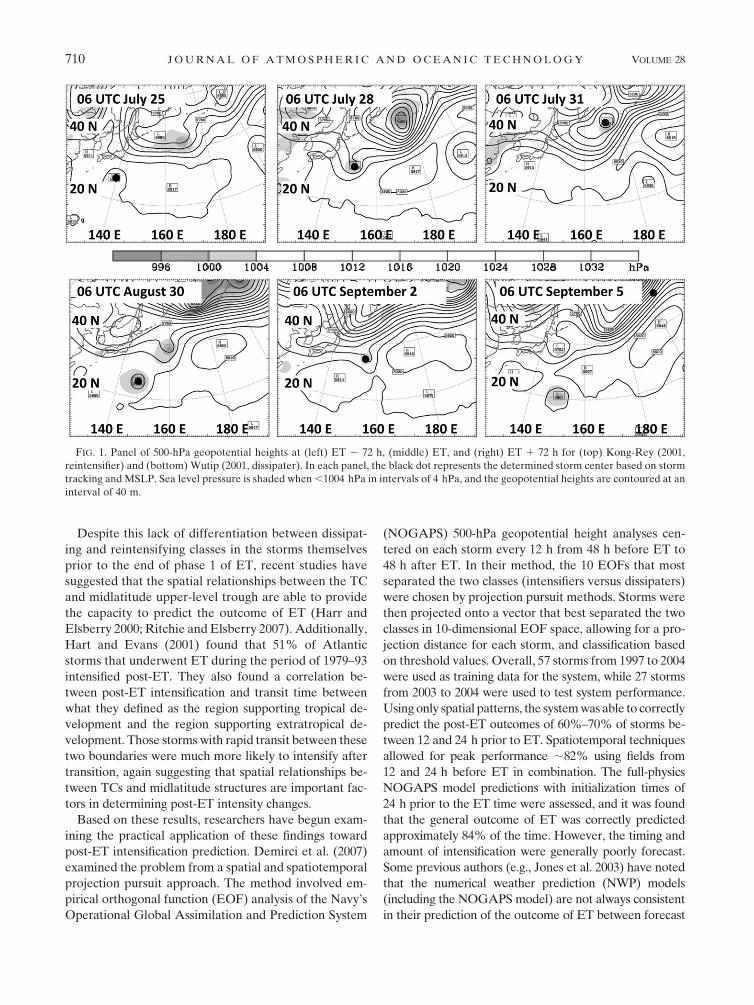
latitudes (Fig. 1). Thus, the structure of all of the storms
moving poleward tends to appear quite similar prior to
the second stage of ET.
Corresponding author address: Dr. E. A. Ritchie, P.O. Box 210081,
Department of Atmospheric Sciences, University of Arizona, Tuc-
son, AZ 85721-0081.
E-mail: [email protected]
MAY 2011 F E L K E R E T A L . 709
DOI: 10.1175/2010JTECHA1449.1
� 2011 American Meteorological Society
Despite this lack of differentiation between dissipat-
ing and reintensifying classes in the storms themselves
prior to the end of phase 1 of ET, recent studies have
suggested that the spatial relationships between the TC
and midlatitude upper-level trough are able to provide
the capacity to predict the outcome of ET (Harr and
Elsberry 2000; Ritchie and Elsberry 2007). Additionally,
Hart and Evans (2001) found that 51% of Atlantic
storms that underwent ET during the period of 1979–93
intensified post-ET. They also found a correlation be-
tween post-ET intensification and transit time between
what they defined as the region supporting tropical de-
velopment and the region supporting extratropical de-
velopment. Those storms with rapid transit between these
two boundaries were much more likely to intensify after
transition, again suggesting that spatial relationships be-
tween TCs and midlatitude structures are important fac-
tors in determining post-ET intensity changes.
Based on these results, researchers have begun exam-
ining the practical application of these findings toward
post-ET intensification prediction. Demirci et al. (2007)
examined the problem from a spatial and spatiotemporal
projection pursuit approach. The method involved em-
pirical orthogonal function (EOF) analysis of the Navy’s
Operational Global Assimilation and Prediction System
(NOGAPS) 500-hPa geopotential height analyses cen-
tered on each storm every 12 h from 48 h before ET to
48 h after ET. In their method, the 10 EOFs that most
separated the two classes (intensifiers versus dissipaters)
were chosen by projection pursuit methods. Storms were
then projected onto a vector that best separated the two
classes in 10-dimensional EOF space, allowing for a pro-
jection distance for each storm, and classification based
on threshold values. Overall, 57 storms from 1997 to 2004
were used as training data for the system, while 27 storms
from 2003 to 2004 were used to test system performance.
Using only spatial patterns, the system was able to correctly
predict the post-ET outcomes of 60%–70% of storms be-
tween 12 and 24 h prior to ET. Spatiotemporal techniques
allowed for peak performance ;82% using fields from
12 and 24 h before ET in combination. The full-physics
NOGAPS model predictions with initialization times of
24 h prior to the ET time were assessed, and it was found
that the general outcome of ET was correctly predicted
approximately 84% of the time. However, the timing and
amount of intensification were generally poorly forecast.
Some previous authors (e.g., Jones et al. 2003) have noted
that the numerical weather prediction (NWP) models
(including the NOGAPS model) are not always consistent
in their prediction of the outcome of ET between forecast
FIG. 1. Panel of 500-hPa geopotential heights at (left) ET 2 72 h, (middle) ET, and (right) ET 1 72 h for (top) Kong-Rey (2001,
reintensifier) and (bottom) Wutip (2001, dissipater). In each panel, the black dot represents the determined storm center based on storm
tracking and MSLP. Sea level pressure is shaded when ,1004 hPa in intervals of 4 hPa, and the geopotential heights are contoured at an
interval of 40 m.
710 J O U R N A L O F A T M O S P H E R I C A N D O C E A N I C T E C H N O L O G Y VOLUME 28
cycles leading up to the ET time, although typically their
performance improves within about 24 h of the ET time. A
distinct, statistically based prediction technique [such as the
Demirci et al. (2007) technique] that had predictability at,
for example, a 72-h lead time would lend confidence to the
NWP forecast by either supporting or disputing the basic
forecast of ET outcome and providing useful additional
information to the forecaster.
In this study, we have built on the work of Demirci et al.
(2007) by looking at transitioning storms in high dimen-
sional spaces and using advanced support vector machine
(SVM) classification techniques in the hope of further
increasing the range of forecast accuracy with respect to
post-ET intensity change classification. The format of the
paper is as follows. The methodology behind this new
classification system is described in section 2. Some pre-
liminary results are presented in section 3 using spatial
patterns in one chosen atmospheric variable to show the
potential effectiveness of such a pattern recognition sys-
tem for forecasting the eventual outcome of ET up to 72 h
in advance. These results, along with future work, are
discussed in section 4.
2. Methodology
The overall method for this post-ET intensity classi-
fication system relies on a number of steps. The first of
these steps comprise preprocessing of the data for train-
ing purposes, and would not need to be repeated in a
forecasting situation. The overall outline of the method-
ology is as follows: 1) track the storms and diagnose the
structural evolution through time to determine the timing
of the ET, as well as the positions and post-ET intensity;
2) classify the storm based on intensity evolution; 3)
preprocess the storm data; and 4) apply the SVM, select
the model, and evaluate the error.
a. Tracking individual storms and ET timedetermination
Overall, 108 western North Pacific tropical cyclones that
underwent extratropical transition between January 2000
and December 2008 were identified and processed. For
each storm, ET time was defined as the first time that the
storm appeared as an open wave on the midlatitude trough
in the Global Forecast System (GFS) final analysis (FNL)
500-hPa geopotential height analyses using a 20-m contour
(e.g., Fig. 1). This was the definition for ‘‘ET time’’ that was
used in Demirci et al. (2007) and corresponded well to the
end of the transformation time of ET in Klein et al. (2000).
It was after this ET time that reintensification or dissipa-
tion of the TC would occur. A study by Kofron et al.
(2010a) demonstrated that although the ‘‘open wave’’
definition could not be readily automated, it was objective,
and did correctly identify all of the TCs that were begin-
ning ET in their study.
After an ET time was established for each storm, the
storm was then tracked in the model analysis from 72 h
before the ET time (ET 2 72 h) to 72 h after the ET time
(ET 1 72 h) at an interval of 6 h. Because the storm center
in the analysis might not exactly match the location in the
best-track archives, an automated procedure was devel-
oped that used the best-track location as the first-guess
position in the analysis field and then searched an area 658
latitude for the actual minimum sea level pressure in the
analysis. The center location chosen by the system was
checked and verified visually in case there were multiple
low pressure centers within the search area. These tracking
data were archived and used to center the model data
around the storm center at a distance of 6308 longitude,
and 6258 latitude, and to save pressure-level fields of all of
the available atmospheric model variables for each storm
at each relative ET time. Thus, each storm variable field
for each relative ET time was composed of 3111 (618 3
518) gridpoint values, corresponding to the storm itself and
its surrounding environment before, during, and after ET.
An extension of Demirci et al. (2007) showed that
a multivariate strategy for ET projection-pursuit pre-
diction had higher potential for success in forecasting the
outcome of ET than pursuing a single variable (Demirci
2006). Rather than prejudice the process by determining
a priori that particular fields (e.g., Harr and Elsberry 2000;
Ritchie and Elsberry 2003, 2007) would be the most suc-
cessful discriminators of ET outcome, all of the basic raw
model output fields from the GFS FNL model and the
potential temperature and equivalent potential tempera-
ture were tested using an SVM classifier and five testing
sets of storms. Based on the results of these quick-look
analyses, several variables were chosen for their success in
correctly discriminating between reintensifying and dissi-
pating TCs. These variables included geopotential heights
at 500 hPa (as used in Demirci et al. 2007), vertical ve-
locity at 600 and 100 hPa, meridional winds at 100 hPa,
and potential temperature and equivalent potential tem-
perature at 850 hPa. The greatest success was achieved
using 850-hPa potential temperature, and the differences
between the features in the two classes (reintensifying and
dissipating) could be easily understood in terms of the
evolution of the atmospheric circulation patterns in the
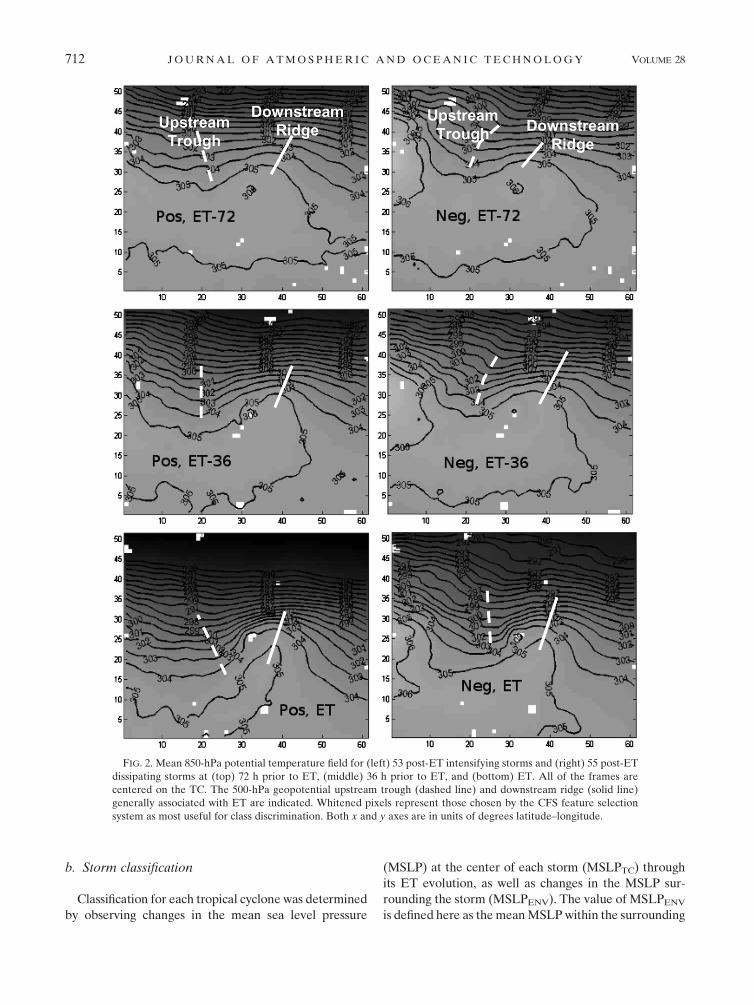
potential temperature fields. In particular, 850-hPa po-
tential temperature fields captured the structure of the TC
itself, but perhaps more importantly they also captured the
location and intensity of frontal zones and associated
midlatitude features (Fig. 2). Therefore, these potential
temperature fields were chosen as the inputs of choice for
demonstrating the potential of the classification technique
outlined in this paper.
MAY 2011 F E L K E R E T A L . 711
b. Storm classification
Classification for each tropical cyclone was determined
by observing changes in the mean sea level pressure
(MSLP) at the center of each storm (MSLPTC) through
its ET evolution, as well as changes in the MSLP sur-
rounding the storm (MSLPENV). The value of MSLPENV
is defined here as the mean MSLP within the surrounding
FIG. 2. Mean 850-hPa potential temperature field for (left) 53 post-ET intensifying storms and (right) 55 post-ET
dissipating storms at (top) 72 h prior to ET, (middle) 36 h prior to ET, and (bottom) ET. All of the frames are
centered on the TC. The 500-hPa geopotential upstream trough (dashed line) and downstream ridge (solid line)
generally associated with ET are indicated. Whitened pixels represent those chosen by the CFS feature selection
system as most useful for class discrimination. Both x and y axes are in units of degrees latitude–longitude.
712 J O U R N A L O F A T M O S P H E R I C A N D O C E A N I C T E C H N O L O G Y VOLUME 28
environment (between all 3111 grid points). Because the
TC central pressures in the FNL analyses are most
probably only accurate to within a few hectopascals at
best, some freedom was introduced into the criteria for
reintensification after ET. Storms for which MSLPENV–
MSLPTC increased more than 3 hPa in the time interval
starting at ET 6 6 h and ending in the period between
ET 1 36 h and ET 1 72 h were categorized as positive
storms; that is, storms that intensified substantially post-
ET. The reasoning behind the time bounds around ET
and following ET are as follows: 1) by including the two
times adjacent to ET (i.e., ET 6 6 h), the definition is
relaxed in case there are some storms for which the time
of the open wave and the time of the maximum central
pressure do not exactly coincide; and 2) by only consid-
ering intensity between ET 1 36 h and ET 1 72 h as
post-ET time, we prevent storms that only intensified
briefly after our defined ET from being considered as
reintensifying (positive) storms. All of the other storms
were categorized as dissipating (negative) storms. This
system of categorization resulted in 53 positive storms
and 55 negative storms overall.
c. Data preprocessing
Because of the large amount of data available in the
form of 3111 spatial data points (the initial set of features
available for classification), the first preprocessing step
was to reduce the dimensionality of the inputs using fea-
ture selection, while attempting to best retain information
content that would be useful for classification. Because it
has been observed in practice that added features tend to
degrade classification performance in situations where the
number of cases is small relative to the number of features
(Jain et al. 2000), and because the dataset in use here is
comprised of only 108 cases and a total of 3111 features, it
was decided that the dimensionality of the feature set
must be reduced before classification. For this task the
correlation-based feature selection (CFS) method devel-
oped by Hall (1999, 2000) was chosen. The main premise
behind this selection method is that the features that are
most effective for classification are those that are most
highly correlated with the classes (intensifiers and dissi-
paters), and at the same time are least correlated with
other features. The method is therefore used to choose a
subset of features that best represent these qualities. For
this study, a modified forward selection version of the
CFS method, with the dot product representing the re-
lationship between variables, was used; the system first
chooses the best individual feature based on the metric
Ms
5k 3 r
cfffiffiffiffiffiffiffiffiffiffiffiffiffiffiffiffiffiffiffiffiffiffiffiffiffiffiffiffiffiffiffiffiffiffiffiffiffiffik 1 k(k� 1) 3 r
ff
p , (1)
where Ms is the merit metric, k is the number of features
in the subset, rcf is the mean of the dot product between
features and classes, and rff is the mean of the dot product
between the features themselves. Subsequently, the first
chosen feature is matched with each other feature out of
the set of 3111 spatial model grid points, and Ms is recal-
culated for each set of two features. The feature combi-
nation that maximizes Ms is then chosen iteratively up
until a chosen number of input features is reached.
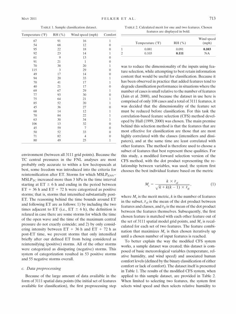
To better explain the way the modified CFS system
works, a sample dataset was created; this dataset is com-
posed of basic meteorological variables (temperature, rel-
ative humidity, and wind speed) and associated human
comfort levels (defined by the binary classification of either
comfort or lack of comfort). The dataset itself is presented
in Table 1. The results of the modified CFS system, when
applied to this sample dataset, are provided in Table 2.
When limited to selecting two features, the system first
selects wind speed and then selects relative humidity to
TABLE 1. Sample classification dataset.
Temperature (8F) RH (%) Wind speed (mph) Comfort
67 91 16 1
54 68 12 0
95 22 18 0
92 23 14 1
61 9 13 0
91 21 1 0
70 38 20 1
115 3 29 0
49 17 14 0
94 20 33 1
70 41 17 1
40 21 17 0
69 67 29 1
77 93 30 0
75 64 21 1
85 52 20 1
45 36 27 0
68 14 12 1
70 84 22 1
63 30 34 1
106 13 32 0
45 59 7 0
50 52 33 0
71 82 4 0
80 49 25 1
TABLE 2. Calculated merit for one and two features. Chosen
features are displayed in bold.
Temperature (8F) RH (%)
Wind speed
(mph)
1 0.081 0.091 0.103
2 0.103 0.111 NA
MAY 2011 F E L K E R E T A L . 713
best complement it, based on highest merit. This same
methodology is used to select spatial grid points from the
3111 available.
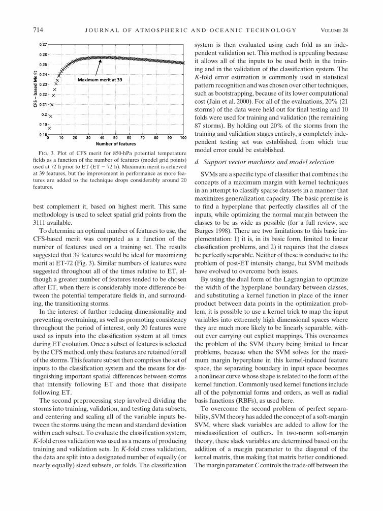
To determine an optimal number of features to use, the
CFS-based merit was computed as a function of the
number of features used on a training set. The results
suggested that 39 features would be ideal for maximizing
merit at ET-72 (Fig. 3). Similar numbers of features were
suggested throughout all of the times relative to ET, al-
though a greater number of features tended to be chosen
after ET, when there is considerably more difference be-
tween the potential temperature fields in, and surround-
ing, the transitioning storms.
In the interest of further reducing dimensionality and
preventing overtraining, as well as promoting consistency
throughout the period of interest, only 20 features were
used as inputs into the classification system at all times
during ET evolution. Once a subset of features is selected
by the CFS method, only these features are retained for all
of the storms. This feature subset then comprises the set of
inputs to the classification system and the means for dis-
tinguishing important spatial differences between storms
that intensify following ET and those that dissipate
following ET.
The second preprocessing step involved dividing the
storms into training, validation, and testing data subsets,
and centering and scaling all of the variable inputs be-
tween the storms using the mean and standard deviation
within each subset. To evaluate the classification system,
K-fold cross validation was used as a means of producing
training and validation sets. In K-fold cross validation,
the data are split into a designated number of equally (or
nearly equally) sized subsets, or folds. The classification
system is then evaluated using each fold as an inde-
pendent validation set. This method is appealing because
it allows all of the inputs to be used both in the train-
ing and in the validation of the classification system. The
K-fold error estimation is commonly used in statistical
pattern recognition and was chosen over other techniques,
such as bootstrapping, because of its lower computational
cost (Jain et al. 2000). For all of the evaluations, 20% (21
storms) of the data were held out for final testing and 10
folds were used for training and validation (the remaining
87 storms). By holding out 20% of the storms from the
training and validation stages entirely, a completely inde-
pendent testing set was established, from which true
model error could be established.
d. Support vector machines and model selection
SVMs are a specific type of classifier that combines the
concepts of a maximum margin with kernel techniques
in an attempt to classify sparse datasets in a manner that
maximizes generalization capacity. The basic premise is
to find a hyperplane that perfectly classifies all of the
inputs, while optimizing the normal margin between the
classes to be as wide as possible (for a full review, see
Burges 1998). There are two limitations to this basic im-
plementation: 1) it is, in its basic form, limited to linear
classification problems, and 2) it requires that the classes
be perfectly separable. Neither of these is conducive to the
problem of post-ET intensity change, but SVM methods
have evolved to overcome both issues.
By using the dual form of the Lagrangian to optimize
the width of the hyperplane boundary between classes,
and substituting a kernel function in place of the inner
product between data points in the optimization prob-
lem, it is possible to use a kernel trick to map the input
variables into extremely high dimensional spaces where
they are much more likely to be linearly separable, with-
out ever carrying out explicit mappings. This overcomes
the problem of the SVM theory being limited to linear
problems, because when the SVM solves for the maxi-
mum margin hyperplane in this kernel-induced feature
space, the separating boundary in input space becomes
a nonlinear curve whose shape is related to the form of the
kernel function. Commonly used kernel functions include
all of the polynomial forms and orders, as well as radial
basis functions (RBFs), as used here.
To overcome the second problem of perfect separa-
bility, SVM theory has added the concept of a soft-margin
SVM, where slack variables are added to allow for the
misclassification of outliers. In two-norm soft-margin
theory, these slack variables are determined based on the
addition of a margin parameter to the diagonal of the
kernel matrix, thus making that matrix better conditioned.
The margin parameter C controls the trade-off between the
FIG. 3. Plot of CFS merit for 850-hPa potential temperature
fields as a function of the number of features (model grid points)
used at 72 h prior to ET (ET 2 72 h). Maximum merit is achieved
at 39 features, but the improvement in performance as more fea-
tures are added to the technique drops considerably around 20
features.
714 J O U R N A L O F A T M O S P H E R I C A N D O C E A N I C T E C H N O L O G Y VOLUME 28
cost of misclassification and the width of the margin be-
tween classes. Unfortunately, there is no robust method for
determining an appropriate value for C, and so a range of
values must be tested in order to determine which results in
the best model. Therefore, model selection for SVMs is an
iterative process of varying both the kernel function pa-
rameters and C together, and determining through cross
validation which combinations result in the best general-
ization performance for the classifier.
In this study, an RBF kernel function is used, as
follows:
K(xi, x
j) 5 ekxi
�xjk2/2 3 s2
, (2)
where xi and xj are individual data point vectors and s is
a parameter that controls the areal influence of each data
point. Both the margin parameter and sigma influence the
number of support vectors, which are chosen by the
trained SVM. The support vectors are those observations
(storms in this case), which, if removed, would alter the
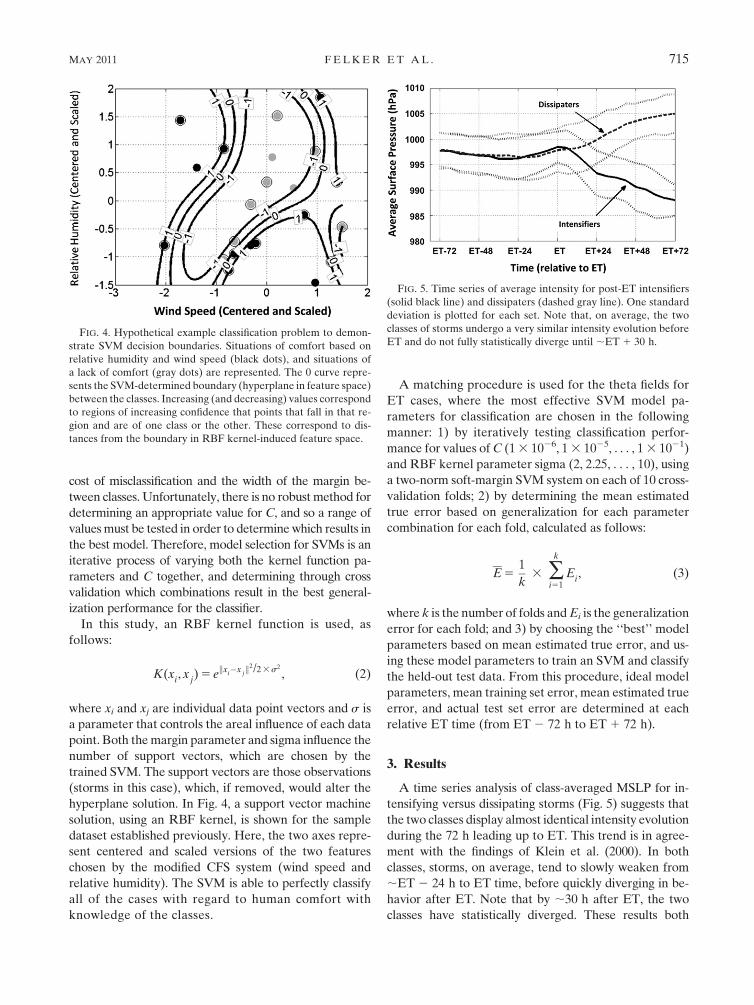
hyperplane solution. In Fig. 4, a support vector machine
solution, using an RBF kernel, is shown for the sample
dataset established previously. Here, the two axes repre-
sent centered and scaled versions of the two features
chosen by the modified CFS system (wind speed and
relative humidity). The SVM is able to perfectly classify
all of the cases with regard to human comfort with
knowledge of the classes.
A matching procedure is used for the theta fields for
ET cases, where the most effective SVM model pa-
rameters for classification are chosen in the following
manner: 1) by iteratively testing classification perfor-
mance for values of C (1 3 1026, 1 3 1025, . . . , 1 3 1021)
and RBF kernel parameter sigma (2, 2.25, . . . , 10), using
a two-norm soft-margin SVM system on each of 10 cross-
validation folds; 2) by determining the mean estimated
true error based on generalization for each parameter
combination for each fold, calculated as follows:
E 51
k3 �
k
i51E
i, (3)
where k is the number of folds and Ei is the generalization
error for each fold; and 3) by choosing the ‘‘best’’ model
parameters based on mean estimated true error, and us-
ing these model parameters to train an SVM and classify
the held-out test data. From this procedure, ideal model
parameters, mean training set error, mean estimated true
error, and actual test set error are determined at each
relative ET time (from ET 2 72 h to ET 1 72 h).
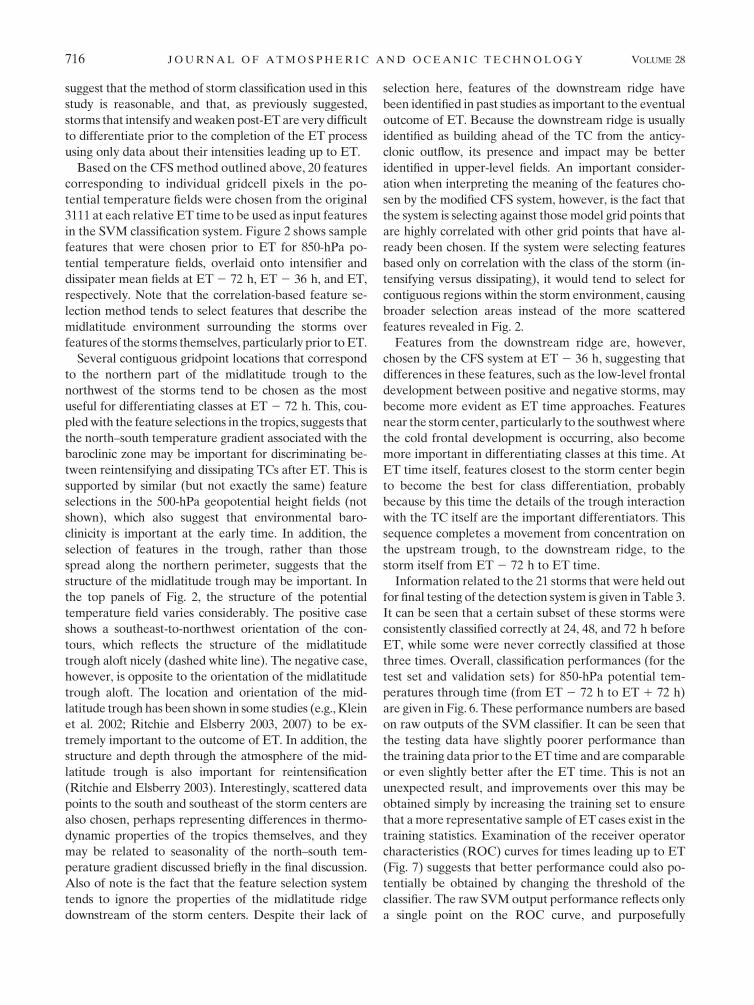
3. Results
A time series analysis of class-averaged MSLP for in-
tensifying versus dissipating storms (Fig. 5) suggests that
the two classes display almost identical intensity evolution
during the 72 h leading up to ET. This trend is in agree-
ment with the findings of Klein et al. (2000). In both
classes, storms, on average, tend to slowly weaken from
;ET 2 24 h to ET time, before quickly diverging in be-
havior after ET. Note that by ;30 h after ET, the two
classes have statistically diverged. These results both
FIG. 4. Hypothetical example classification problem to demon-
strate SVM decision boundaries. Situations of comfort based on
relative humidity and wind speed (black dots), and situations of
a lack of comfort (gray dots) are represented. The 0 curve repre-
sents the SVM-determined boundary (hyperplane in feature space)
between the classes. Increasing (and decreasing) values correspond
to regions of increasing confidence that points that fall in that re-
gion and are of one class or the other. These correspond to dis-
tances from the boundary in RBF kernel-induced feature space.
FIG. 5. Time series of average intensity for post-ET intensifiers
(solid black line) and dissipaters (dashed gray line). One standard
deviation is plotted for each set. Note that, on average, the two
classes of storms undergo a very similar intensity evolution before
ET and do not fully statistically diverge until ;ET 1 30 h.
MAY 2011 F E L K E R E T A L . 715
suggest that the method of storm classification used in this
study is reasonable, and that, as previously suggested,
storms that intensify and weaken post-ET are very difficult
to differentiate prior to the completion of the ET process
using only data about their intensities leading up to ET.
Based on the CFS method outlined above, 20 features
corresponding to individual gridcell pixels in the po-
tential temperature fields were chosen from the original
3111 at each relative ET time to be used as input features
in the SVM classification system. Figure 2 shows sample
features that were chosen prior to ET for 850-hPa po-
tential temperature fields, overlaid onto intensifier and
dissipater mean fields at ET 2 72 h, ET 2 36 h, and ET,
respectively. Note that the correlation-based feature se-
lection method tends to select features that describe the
midlatitude environment surrounding the storms over
features of the storms themselves, particularly prior to ET.
Several contiguous gridpoint locations that correspond
to the northern part of the midlatitude trough to the
northwest of the storms tend to be chosen as the most
useful for differentiating classes at ET 2 72 h. This, cou-
pled with the feature selections in the tropics, suggests that
the north–south temperature gradient associated with the
baroclinic zone may be important for discriminating be-
tween reintensifying and dissipating TCs after ET. This is
supported by similar (but not exactly the same) feature
selections in the 500-hPa geopotential height fields (not
shown), which also suggest that environmental baro-
clinicity is important at the early time. In addition, the
selection of features in the trough, rather than those
spread along the northern perimeter, suggests that the
structure of the midlatitude trough may be important. In
the top panels of Fig. 2, the structure of the potential
temperature field varies considerably. The positive case
shows a southeast-to-northwest orientation of the con-
tours, which reflects the structure of the midlatitude
trough aloft nicely (dashed white line). The negative case,
however, is opposite to the orientation of the midlatitude
trough aloft. The location and orientation of the mid-
latitude trough has been shown in some studies (e.g., Klein
et al. 2002; Ritchie and Elsberry 2003, 2007) to be ex-
tremely important to the outcome of ET. In addition, the
structure and depth through the atmosphere of the mid-
latitude trough is also important for reintensification
(Ritchie and Elsberry 2003). Interestingly, scattered data
points to the south and southeast of the storm centers are
also chosen, perhaps representing differences in thermo-
dynamic properties of the tropics themselves, and they
may be related to seasonality of the north–south tem-
perature gradient discussed briefly in the final discussion.
Also of note is the fact that the feature selection system
tends to ignore the properties of the midlatitude ridge
downstream of the storm centers. Despite their lack of
selection here, features of the downstream ridge have
been identified in past studies as important to the eventual
outcome of ET. Because the downstream ridge is usually
identified as building ahead of the TC from the anticy-
clonic outflow, its presence and impact may be better
identified in upper-level fields. An important consider-
ation when interpreting the meaning of the features cho-
sen by the modified CFS system, however, is the fact that
the system is selecting against those model grid points that
are highly correlated with other grid points that have al-
ready been chosen. If the system were selecting features
based only on correlation with the class of the storm (in-
tensifying versus dissipating), it would tend to select for
contiguous regions within the storm environment, causing
broader selection areas instead of the more scattered
features revealed in Fig. 2.
Features from the downstream ridge are, however,
chosen by the CFS system at ET 2 36 h, suggesting that
differences in these features, such as the low-level frontal
development between positive and negative storms, may
become more evident as ET time approaches. Features
near the storm center, particularly to the southwest where
the cold frontal development is occurring, also become
more important in differentiating classes at this time. At
ET time itself, features closest to the storm center begin
to become the best for class differentiation, probably
because by this time the details of the trough interaction
with the TC itself are the important differentiators. This
sequence completes a movement from concentration on
the upstream trough, to the downstream ridge, to the
storm itself from ET 2 72 h to ET time.
Information related to the 21 storms that were held out
for final testing of the detection system is given in Table 3.
It can be seen that a certain subset of these storms were
consistently classified correctly at 24, 48, and 72 h before
ET, while some were never correctly classified at those
three times. Overall, classification performances (for the
test set and validation sets) for 850-hPa potential tem-
peratures through time (from ET 2 72 h to ET 1 72 h)
are given in Fig. 6. These performance numbers are based
on raw outputs of the SVM classifier. It can be seen that
the testing data have slightly poorer performance than
the training data prior to the ET time and are comparable
or even slightly better after the ET time. This is not an
unexpected result, and improvements over this may be
obtained simply by increasing the training set to ensure
that a more representative sample of ET cases exist in the
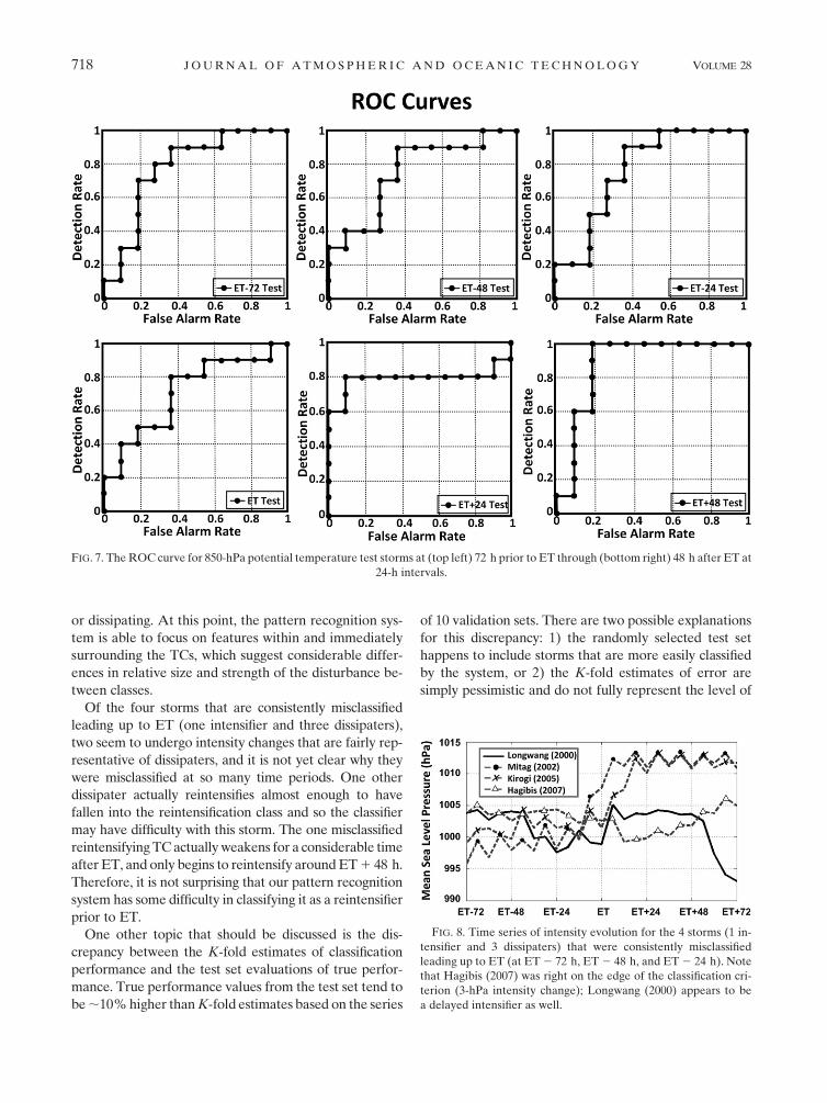
training statistics. Examination of the receiver operator
characteristics (ROC) curves for times leading up to ET
(Fig. 7) suggests that better performance could also po-
tentially be obtained by changing the threshold of the
classifier. The raw SVM output performance reflects only
a single point on the ROC curve, and purposefully
716 J O U R N A L O F A T M O S P H E R I C A N D O C E A N I C T E C H N O L O G Y VOLUME 28
allowing a certain amount of false detection may provide
for a more robust detection system overall. For example,
one could potentially achieve a positive detection rate of
80%, at 72 h prior to the ET time if a false alarm rate of
27% were an acceptable risk (Fig. 7). Despite this fact,
and even using raw SVM output, this prediction system
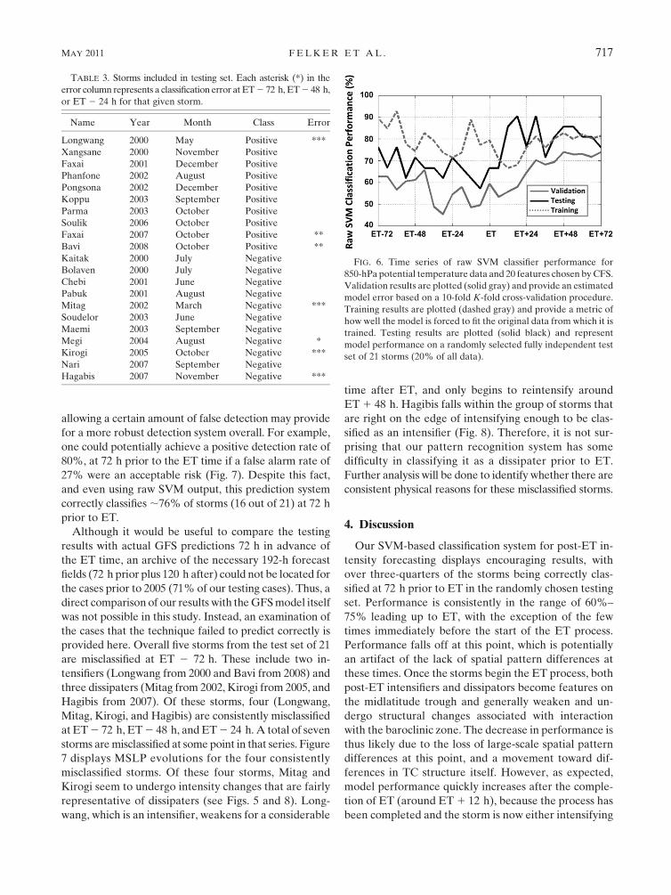
correctly classifies ;76% of storms (16 out of 21) at 72 h
prior to ET.
Although it would be useful to compare the testing
results with actual GFS predictions 72 h in advance of
the ET time, an archive of the necessary 192-h forecast
fields (72 h prior plus 120 h after) could not be located for
the cases prior to 2005 (71% of our testing cases). Thus, a
direct comparison of our results with the GFS model itself
was not possible in this study. Instead, an examination of
the cases that the technique failed to predict correctly is
provided here. Overall five storms from the test set of 21
are misclassified at ET 2 72 h. These include two in-
tensifiers (Longwang from 2000 and Bavi from 2008) and
three dissipaters (Mitag from 2002, Kirogi from 2005, and
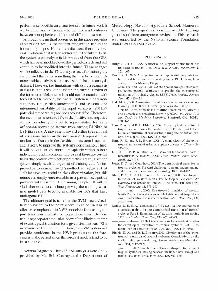
Hagibis from 2007). Of these storms, four (Longwang,
Mitag, Kirogi, and Hagibis) are consistently misclassified
at ET 2 72 h, ET 2 48 h, and ET 2 24 h. A total of seven
storms are misclassified at some point in that series. Figure
7 displays MSLP evolutions for the four consistently
misclassified storms. Of these four storms, Mitag and
Kirogi seem to undergo intensity changes that are fairly
representative of dissipaters (see Figs. 5 and 8). Long-
wang, which is an intensifier, weakens for a considerable
time after ET, and only begins to reintensify around
ET 1 48 h. Hagibis falls within the group of storms that
are right on the edge of intensifying enough to be clas-
sified as an intensifier (Fig. 8). Therefore, it is not sur-
prising that our pattern recognition system has some
difficulty in classifying it as a dissipater prior to ET.
Further analysis will be done to identify whether there are
consistent physical reasons for these misclassified storms.
4. Discussion
Our SVM-based classification system for post-ET in-
tensity forecasting displays encouraging results, with
over three-quarters of the storms being correctly clas-
sified at 72 h prior to ET in the randomly chosen testing
set. Performance is consistently in the range of 60%–
75% leading up to ET, with the exception of the few
times immediately before the start of the ET process.
Performance falls off at this point, which is potentially
an artifact of the lack of spatial pattern differences at
these times. Once the storms begin the ET process, both
post-ET intensifiers and dissipators become features on
the midlatitude trough and generally weaken and un-
dergo structural changes associated with interaction
with the baroclinic zone. The decrease in performance is
thus likely due to the loss of large-scale spatial pattern
differences at this point, and a movement toward dif-
ferences in TC structure itself. However, as expected,
model performance quickly increases after the comple-
tion of ET (around ET 1 12 h), because the process has
been completed and the storm is now either intensifying
FIG. 6. Time series of raw SVM classifier performance for
850-hPa potential temperature data and 20 features chosen by CFS.
Validation results are plotted (solid gray) and provide an estimated
model error based on a 10-fold K-fold cross-validation procedure.
Training results are plotted (dashed gray) and provide a metric of
how well the model is forced to fit the original data from which it is
trained. Testing results are plotted (solid black) and represent
model performance on a randomly selected fully independent test
set of 21 storms (20% of all data).
TABLE 3. Storms included in testing set. Each asterisk (*) in the
error column represents a classification error at ET 2 72 h, ET 2 48 h,
or ET 2 24 h for that given storm.
Name Year Month Class Error
Longwang 2000 May Positive ***
Xangsane 2000 November Positive
Faxai 2001 December Positive
Phanfone 2002 August Positive
Pongsona 2002 December Positive
Koppu 2003 September Positive
Parma 2003 October Positive
Soulik 2006 October Positive
Faxai 2007 October Positive **
Bavi 2008 October Positive **
Kaitak 2000 July Negative
Bolaven 2000 July Negative
Chebi 2001 June Negative
Pabuk 2001 August Negative
Mitag 2002 March Negative ***
Soudelor 2003 June Negative
Maemi 2003 September Negative
Megi 2004 August Negative *
Kirogi 2005 October Negative ***
Nari 2007 September Negative
Hagabis 2007 November Negative ***
MAY 2011 F E L K E R E T A L . 717
or dissipating. At this point, the pattern recognition sys-
tem is able to focus on features within and immediately
surrounding the TCs, which suggest considerable differ-
ences in relative size and strength of the disturbance be-
tween classes.
Of the four storms that are consistently misclassified
leading up to ET (one intensifier and three dissipaters),
two seem to undergo intensity changes that are fairly rep-
resentative of dissipaters, and it is not yet clear why they
were misclassified at so many time periods. One other
dissipater actually reintensifies almost enough to have
fallen into the reintensification class and so the classifier
may have difficulty with this storm. The one misclassified
reintensifying TC actually weakens for a considerable time
after ET, and only begins to reintensify around ET 1 48 h.
Therefore, it is not surprising that our pattern recognition
system has some difficulty in classifying it as a reintensifier
prior to ET.
One other topic that should be discussed is the dis-
crepancy between the K-fold estimates of classification
performance and the test set evaluations of true perfor-
mance. True performance values from the test set tend to
be ;10% higher than K-fold estimates based on the series
of 10 validation sets. There are two possible explanations
for this discrepancy: 1) the randomly selected test set
happens to include storms that are more easily classified
by the system, or 2) the K-fold estimates of error are
simply pessimistic and do not fully represent the level of
FIG. 7. The ROC curve for 850-hPa potential temperature test storms at (top left) 72 h prior to ET through (bottom right) 48 h after ET at
24-h intervals.
FIG. 8. Time series of intensity evolution for the 4 storms (1 in-
tensifier and 3 dissipaters) that were consistently misclassified
leading up to ET (at ET 2 72 h, ET 2 48 h, and ET 2 24 h). Note
that Hagibis (2007) was right on the edge of the classification cri-
terion (3-hPa intensity change); Longwang (2000) appears to be
a delayed intensifier as well.
718 J O U R N A L O F A T M O S P H E R I C A N D O C E A N I C T E C H N O L O G Y VOLUME 28
performance possible on a true test set. In future work it
will be important to examine whether this trend continues
between atmospheric variables and different test sets.
Although the method presented in this paper provides
encouraging results for pattern recognition use in the
forecasting of post-ET reintensification, there are sev-
eral limitations that will be addressed in the future. First,
the system uses analysis fields produced from the GFS,
which has been modified over the period of study and will
continue to be modified into the future. These changes
will be reflected in the FNL analyses used for training the
system, and this is not something that can be rectified. A
more stable analysis set to use would be a reanalysis
dataset. However, the limitations with using a reanalysis
dataset is that it would not match the current version of
the forecast model, and so it could not be matched with
forecast fields. Second, the overall system is highly non-
stationary (the earth’s atmosphere), and seasonal and
interannual variability of the input variables (850-hPa
potential temperature) are not accounted for. Therefore,
the mean that is removed from the positive and negative
storms individually may not be representative for many
off-season storms or storms from strong El Nino or
La Nina years. A movement toward either the removal
of a seasonal mean or the inclusion of temporal infor-
mation as a feature in the classification system is needed,
and is likely to improve the system’s performance. Third,
it will be vital to test more atmospheric variables both
individually and in combination to see if there are certain
fields that provide even better predictive ability. Last, the
system simply needs a larger set of training data for im-
proved performance. The CFS method has suggested that
;40 features are useful in class discrimination, but this
number is simply unreasonable in a pattern recognition
problem with less than 100 training samples. It will be
vital, therefore, to continue growing the training set as
new model data become available for TCs that have
undergone ET.
The ultimate goal is to refine the SVM-based classi-
fication system to the point where it can be used as an
effective complement to NWP models in forecasting the
post-transition intensity of tropical cyclones. By con-
tributing a separate statistical view of the likely outcome
of extratropical transition for a given storm at least 72-h
in advance of the common ET time, the SVM system will
provide confidence in the NWP products to the fore-
casters in the period when the forecast models tend to be
least reliable.
Acknowledgments. The GFS FNL analyses were kindly
provided by Mr. Bob Creasey at the Department of
Meteorology, Naval Postgraduate School, Monterey,
California. The paper has been improved by the sug-
gestions of three anonymous reviewers. This research
was supported by the National Science Foundation
under Grant ATM-0730079.
REFERENCES
Burges, C. J. C., 1998: A tutorial on support vector machines
for pattern recognition. Data Min. Knowl. Discovery, 2,121–167.
Demirci, O., 2006: A projection pursuit application to predict ex-
tratropical transition of tropical cyclones. Ph.D. thesis, Uni-
versity of New Mexico, 137 pp.
——, J. S. Tyo, and E. A. Ritchie, 2007: Spatial and spatiotemporal
projection pursuit techniques to predict the extratropical
transition of tropical cyclones. IEEE Trans. Geosci. Remote
Sens., 45, 418–425.
Hall, M. A., 1999: Correlation-based feature selection for machine
learning. Ph.D. thesis, University of Waikato, 198 pp.
——, 2000: Correlation-based feature selection for discrete
and numeric class machine learning. ICML ’00: Proc. 17th
Int. Conf. on Machine Learning, Stanford, CA, ICML,
359–366.
Harr, P. A., and R. L. Elsberry, 2000: Extratropical transition of
tropical cyclones over the western North Pacific. Part I: Evo-
lution of structural characteristics during the transition pro-
cess. Mon. Wea. Rev., 128, 2613–2633.
Hart, R. E., and J. L. Evans, 2001: A climatology of the extra-
tropical transition of Atlantic tropical cyclones. J. Climate, 14,
546–564.
Jain, A. K., R. P. W. Duin, and J. Mao, 2000: Statistical pattern
recognition: A review. IEEE Trans. Pattern Anal. Mach.
Intell., 22, 4–37.
Jones, S. C., and Coauthors, 2003: The extratropical transition of
tropical cyclones: Forecast challenges, current understanding,
and future directions. Wea. Forecasting, 18, 1052–1092.
Klein, P. M., P. A. Harr, and R. L. Elsberry, 2000: Extratropical
transition of western North Pacific tropical cyclones: An
overview and conceptual model of the transformation stage.
Wea. Forecasting, 15, 373–395.
——, ——, and ——, 2002: Extratropical transition of western
North Pacific tropical cyclones: Midlatitude and tropical cy-
clone contributions to reintensification. Mon. Wea. Rev., 130,2240–2259.
Kofron, D. E., E. A. Ritchie, and J. S. Tyo, 2010a: Determination of
a consistent time for the extratropical transition of tropical
cyclones Part I: Examination of existing methods for finding
‘‘ET time’’. Mon. Wea. Rev., 138, 4328–4343.
——, ——, and ——, 2010b: Determination of a consistent time for
the extratropical transition of tropical cyclones Part II: Po-
tential vorticity metrics. Mon. Wea. Rev., 138, 4344–4361.
Ritchie, E. A., and R. L. Elsberry, 2003: Simulations of the extra-
tropical transition of tropical cyclones: Contributions by the
midlatitude upper-level trough to reintensification. Mon. Wea.
Rev., 131, 2112–2128.
——, and ——, 2007: Simulations of the extratropical transition of
tropical cyclones: Phasing between the upper-level trough and
tropical cyclones. Mon. Wea. Rev., 135, 862–876.
MAY 2011 F E L K E R E T A L . 719