forecasting models for cost evolution of network components · forecasting models for cost...
TRANSCRIPT

19. okt. 2004 Telenor 1
Forecasting models for cost evolution of network components
and
Risk analysis based on uncertainties in demand forecasts
and cost predictions
Kjell StordahlTelenor Networks

19. okt. 2004 Telenor 2
Forecasting models for cost evolution of network components
Kjell StordahlTelenor Networks

19. okt. 2004 Telenor 3
Agenda
� Write and Crawford’s learning curve model
� The extended learning curve model
� Discussion of different type of parameters in the
models
� Examples
� Conclusion on cost prediction models
19. okt. 2004 Telenor 4
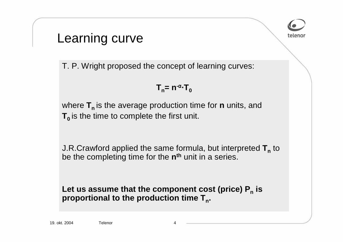
Learning curve
T. P. Wright proposed the concept of learning curves:
Tn= n-αααα·T0
where Tn is the average production time for n units, and T0 is the time to complete the first unit.
J.R.Crawford applied the same formula, but interpreted Tn to be the completing time for the nth unit in a series.
Let us assume that the component cost (price) Pn is proportional to the production time Tn.

19. okt. 2004 Telenor 5
Learning curve coefficient K
Pn= n-αααα P0
Pn is the average cost for the nth unit.
The learning curve coefficient is defined by:
P2n= K · Pn
ThenK= (2) -αααα
α= α= α= α= −−−−log2 K

19. okt. 2004 Telenor 6
Relevant K values of different network components
LearningCurveClass K_ValueCivilWorks 100,00%CopperCable 100,00%Electronics 80,00%SitesAndEnclosures 100,00%FibreCable 90,00%Installation (constant) 100,00%AdvancedOpticalComponents 70,00%Installation (decresing) 85,00%OpticalComponents 80,00%
19. okt. 2004 Telenor 7
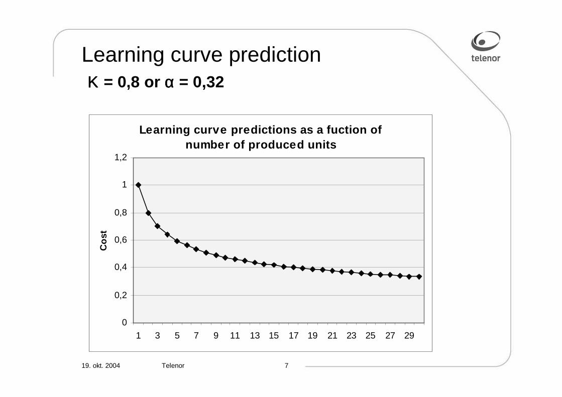
Learning curve predictionΚΚΚΚ = 0,8 or αααα = 0,32
Learning curv e predictions as a fuction of number of produced units
0
0,2
0,4
0,6
0,8
1
1,2
1 3 5 7 9 11 13 15 17 19 21 23 25 27 29
Co
st

19. okt. 2004 Telenor 8
What we need:
Cost as a function of time

19. okt. 2004 Telenor 9
The answer
To combine the learning curves with volume forecastsof components.
P(t) = n(t)−−−−α α α α P(0) = = = = n(t)−−−−log2K P(0)

19. okt. 2004 Telenor 10
The answer
To combine the learning curves with volume forecastsof components.
P(t) = n(t)−−−−α α α α P(0) = = = = n(t)−−−−log2K P(0)
(Olsen , Stordahl 1993) Extended learning curve model is given by inserting a Logistic model into the learning curve model
n(t)= M · [1+ e(a+b·t) ]–γγγγ

19. okt. 2004 Telenor 11
Parameters in the model
� K or α: α: α: α: Learning curve coefficient
� P(0): Production cost, unit no 1
� M: Saturation
� a: Parameter in the Logistic model
� b: Parameter in the Logistic model
� γγγγ: Parameter in the Logistic model

Reformulation of the parameters
The normalized Logistic model is:
nr (t) = n(t)/ M
The aggregated production volume the reference year, 0:
nr (0)
The growth period:
nr (t1) = 0,1 nr (t2) = 0,9
∆∆∆∆T = t1 - t2

19. okt. 2004 Telenor 13
Interpretation of the parameters
0
0,2
0,4
0,6
0,8
1
1,2
t1 t2
0∆∆∆∆T
nr(0)
0
0,2
0,4
0,6
0,8
1
1,2
t1 t2
0∆∆∆∆T
nr(0)
19. okt. 2004 Telenor 14
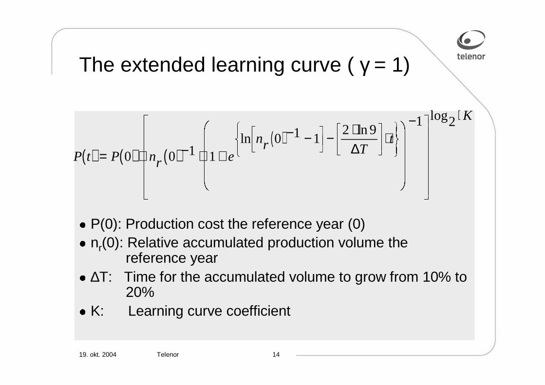
The extended learning curve ( γ = 1)
� P(0): Production cost the reference year (0)
� nr(0): Relative accumulated production volume the reference year
� ∆T: Time for the accumulated volume to grow from 10% to 20%
� K: Learning curve coefficient
( ) ( ) ( )( )
P t P nr enr T
t
K
= ⋅ − ⋅ +
− − − ⋅ ⋅
��
����
��
����
−
��
�
�����
⋅
��
���
�
���
��
���
���
��
���
��
0 0 1 10 1 1
2 91 2
lnln
log
∆

19. okt. 2004 Telenor 15
Cost as a function of Κnr (0)=0.1, ∆∆∆∆T=5
0 1 2 3 4 5 6 7 8 90.1
0.5
0.9
00.10.20.30.40.50.60.70.80.9
1
Relative cost
Project year
Relative cost
K

19. okt. 2004 Telenor 16
Cost as a function of nr(0)∆∆∆∆T = 5, K = 0.8
0 1 2 3 4 5 6 7 8 90.1
0.5
0.9
00.10.20.30.40.50.60.70.80.9
1
Relative cost
Project year
Relative cost
nr (0)

19. okt. 2004 Telenor 17
Cost as a function of ∆Tnr (0) = 0.1, K = 0.8
0 1 2 3 4 5 6 7 82
10
18
00.10.20.30.40.50.60.70.80.9
1
Relative cost
Project year
Relative cost
∆∆∆∆T

19. okt. 2004 Telenor 18
Historical diffusions of selected goods in Canada.
0
10
20
30
40
50
60
70
80
90
100
1953
1956
1962
1966
1975
1982
1985
1987
1989
1991
1993
1995
1997
1999
fixed telephone
Television
Cable
VCR PC
Mobile
Internet

19. okt. 2004 Telenor 19
Historical diffusions of selected goods in Finland.
0
10
20
30
40
50
60
70
80
90
100
1976
1980
1990
1998
2000
2002
Color TV
Freezer
Microwave
Video recorder Dishwasher
MobilePC
Internet
CD player

19. okt. 2004 Telenor 20
Recommended values on the parameters when cost time series are not available
LearningCurveClass K_ValueCivilWorks 100,00%CopperCable 100,00%Electronics 80,00%SitesAndEnclosures 100,00%FibreCable 90,00%Installation (constant) 100,00%AdvancedOpticalComponents 70,00%Installation (decresing) 85,00%OpticalComponents 80,00%
VolumeClass nr(0) ∆T
Emerging_Fast 0,001 5,00Emerging_Medium 0,001 10,00Emerging_Slow 0,001 20,00Emerging_VerySlow 0,001 40,00Mature_Fast 0,1 5,00Mature_Medium 0,1 10,00Mature_Slow 0,1 20,00Mature_VerySlow 0,1 40,00New_Fast 0,01 5,00New_Medium 0,01 10,00New_Slow 0,01 20,00New_VerySlow 0,01 40,00Old_Fast 0,5 5,00Old_Medium 0,5 10,00Old_Slow 0,5 20,00Old_VerySlow 0,5 40,00Straight Line 0,1 1000,00

19. okt. 2004 Telenor 21
Forecasts for ADSL line costs. Estimation: P(2000)= 212 Euro, ∆∆∆∆T=8, n(2000)=0,1%,K=0,736
Forecast model for ADSL line costs
0
50
100
150
200
250
2000 2001 2002 2003 2004 2005 2006 2007 2008 2009 2010
Eu
ro
Model
Data
Forecast model for ADSL line costs
0
50
100
150
200
250
2000 2001 2002 2003 2004 2005 2006 2007 2008 2009 2010
Eu
ro
Model
Data
19. okt. 2004 Telenor 22
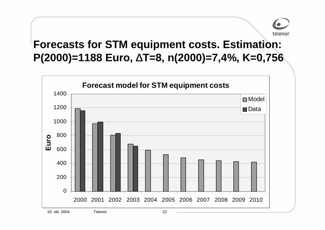
Forecasts for STM equipment costs. Estimation: P(2000)=1188 Euro, ∆∆∆∆T=8, n(2000)=7,4%, K=0,756
Forecast model for STM equipment costs
0
200
400
600
800
1000
1200
1400
2000 2001 2002 2003 2004 2005 2006 2007 2008 2009 2010
Eur
o
Model
Data
Forecast model for STM equipment costs
0
200
400
600
800
1000
1200
1400
2000 2001 2002 2003 2004 2005 2006 2007 2008 2009 2010
Eur
o
Model
Data

19. okt. 2004 Telenor 23
Logistic model with different γ values
-0,2
0
0,2
0,4
0,6
0,8
1
1,2
-10 -5 0 5 10 15 20
0,3
0,5
1
2
4
10
-0,2
0
0,2
0,4
0,6
0,8
1
1,2
-10 -5 0 5 10 15 20
0,3
0,5
1
2
4
10

19. okt. 2004 Telenor 24
The extended learning curve (diff γ)
� P(0): Production cost the reference year (0)
� nr(0): Relative accumulated production volume the reference year
� ∆T: Time for the accumulated volume to grow from 10% to 20%
� K: Learning curve coefficient
� γγγγ: Parameter asymmetry
P t P nr
e
nr
yT
t
K
( ) ( ) ( )
ln ( )ln
log
= ⋅ − ⋅ +
−
− + ⋅
��
��
��
��
���
��
��
��
��
���
−
��
�
��
��
��
��
��
⋅ �
�������������
��
�������������
�
�����
��
�����
��
�������
��������
��
�������
��������
0 0 1 1
0
1
1
2
δ
γ
∆

19. okt. 2004 Telenor 25
Use of the the Extended learning curve model
� RACE 2087/TITAN 1992-1996
� AC 226/OPTIMUM1996-1998
� AC364/TERA1998-2000
� IST-2000-25172 TONIC2000-2002
� ECOSYS / CELTIC 2004-
� Many Eurescom projects
– P306, P413, P614, P901 etc
� Within Telenor and other project partners organizations

19. okt. 2004 Telenor 26
Advantages with the extended learning curve model
� The model makes forecasts of component costs (predictions as a function of time
� The model has the possibility to include both a priori knowledge and statistical information at the same time
� The model can be used to forecast component costs evolution even if no cost observations are known
� The model can be used to forecast component costs based on estimation of the parameters when historical costs are available

19. okt. 2004 Telenor 27
Risk analysis based on uncertainties in demand forecasts
and cost predictions
Kjell StordahlTelenor Networks

19. okt. 2004 Telenor 28
Agenda
� Business case: Roll out of ASDL2+/VDSL
� Adoption rate forecasts
� Evaluation of 6 different roll out scenarios
� Calculation of net present values for the roll out scenarios
� Framework for risk analysis
� Modelling dependency between variables in risk analysis
� Results from risk analysis
� Conclusions

19. okt. 2004 Telenor 29
Important factors for ADSL2+/VDSL roll out
� Broadband demand forecasts
� Substitution effects between broadband technologies
� Competition (Same technology and other technologies)
� Size of the access area
� Distribution of the copper line length
� Standardisation of network technology/components
� Component price and functionality
� Maintenance costs
� Expected ARPU (Average revenue per user)

19. okt. 2004 Telenor 30
Adoption rate forecasts for ADSL2+/VDSL
Adoption rate as a function of delayed introduction
0,0 %
5,0 %
10,0 %
15,0 %
20,0 %
25,0 %
30,0 %
35,0 %
2004 2005 2006 2007 2008 2009 2010
Alone
0 Year delay
1 year delay
2 year delay
3 year delay
4 year delay
5 year delay
6 year delay
19. okt. 2004 Telenor 31
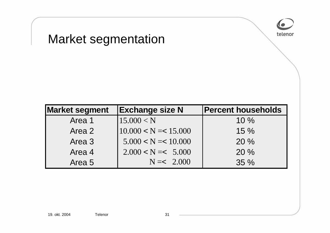
Market segmentation
Market segment Exchange size N Percent householdsArea 1 15.000 < N 10 %Area 2 10.000 < N =< 15.000 15 %Area 3 5.000 < N =< 10.000 20 %Area 4 2.000 < N =< 5.000 20 %Area 5 N =< 2.000 35 %

19. okt. 2004 Telenor 32
Generic case study
Population and coverage
Population 60 000 000Persons per Household (HH) 2,4total number of HH 25 000 000
Area 1 Area 2 Area 3 Area 4 Area 5Distribution of HHs 14 % 21 % 29 % 23 % 13 % 100 %Averagen number of HHs per CO 12 000 8 000 2 600 1 400 400Coverage level 10 % 15 % 20 % 15 % 0 % 60 %HH (in %) within 2 km 75 % 75 % 75 % 75 %Coverage (HP) 2 500 000 3 750 000 5 000 000 3 750 000 15 000 000Total number of HHs in covered echanges 3 333 333 5 000 000 6 666 667 5 000 000Number of upgraded exchanges 278 625 2 564 3 571 7 038Number of HHs in areas without deployment 166 667 250 000 583 333 750 000 3 250 000

19. okt. 2004 Telenor 33
The 6 scenarios studied
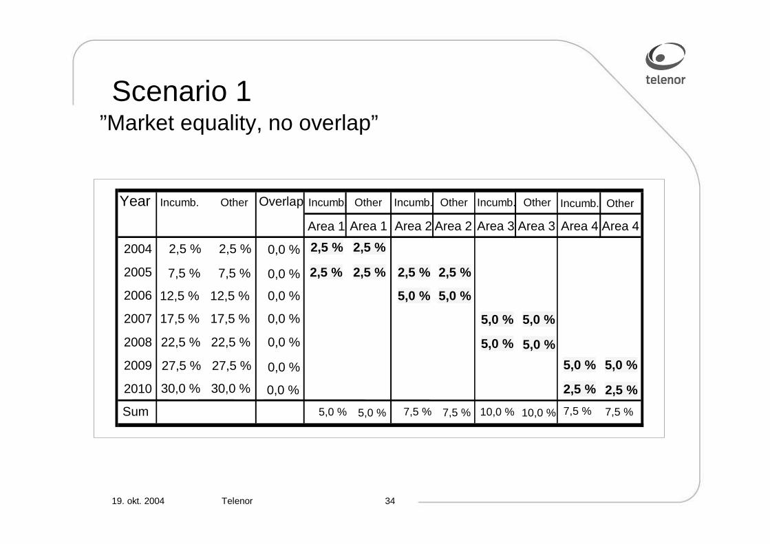
� Scenario 1 – Market equality, no overlap
� Scenario 2 – Market equality, 50% overlap
� Scenario 3 – Market equality, 75% overlap
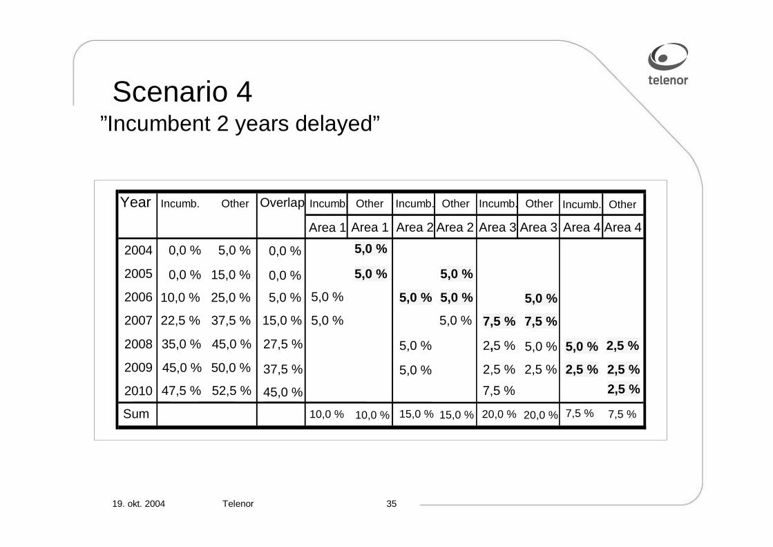
� Scenario 4 – Incumbent 2 years delayed
� Scenario 5 – Incumbent 1 years delayed
� Scenario 6 – Incumbent offensive roll out
19. okt. 2004 Telenor 34
Scenario 1
Year Overlap Incumb. Other
Area 1
2004 2,5 % 2,5 %
2005
2006
2007
2008
2009
2010
Sum
Area 1 Area 2 Area 2 Area 3 Area 3 Area 4 Area 4
Incumb. OtherIncumb. OtherIncumb. Other
2,5 %
2,5 %
2,5 % 2,5 % 2,5 %
5,0 % 5,0 %
5,0 % 5,0 %
5,0 % 5,0 %
5,0 % 5,0 %
2,5 % 2,5 %
Incumb. Other
7,5 %
12,5 %
17,5 %
22,5 %
27,5 %
30,0 %
2,5 %
7,5 %
12,5 %
17,5 %
22,5 %
27,5 %
30,0 %
0,0 %
0,0 %
0,0 %
0,0 %
0,0 %
0,0 %
0,0 %
5,0 % 5,0 % 7,5 % 7,5 % 10,0 % 10,0 % 7,5 % 7,5 %
”Market equality, no overlap”
19. okt. 2004 Telenor 35
Scenario 4
Year Overlap Incumb. Other
Area 1
2004 0,0 %
2005
2006
2007
2008
2009
2010
Sum
Area 1 Area 2 Area 2 Area 3 Area 3 Area 4 Area 4
Incumb. OtherIncumb. OtherIncumb. Other
5,0 %
5,0 % 5,0 %
5,0 % 5,0 %
7,5 % 7,5 %
2,5 % 5,0 %
2,5 % 2,5 %
Incumb. Other
0,0 %
10,0 %
22,5 %
35,0 %
45,0 %
47,5 %
5,0 %
15,0 %
25,0 %
37,5 %
45,0 %
50,0 %
52,5 %
0,0 %
0,0 %
5,0 %
15,0 %
27,5 %
37,5 %
45,0 %
10,0 % 10,0 % 15,0 % 15,0 % 20,0 % 20,0 % 7,5 % 7,5 %
5,0 %
5,0 %
5,0 % 5,0 % 2,5 %
5,0 %
2,5 % 2,5 %
7,5 %
5,0 %
5,0 %
2,5 %
”Incumbent 2 years delayed”

19. okt. 2004 Telenor 36
TheThe business case business case approachapproach::
NPVNPV IRRIRR PaybackPeriod
PaybackPeriod
Economic Inputs
Cash flows, Profit & loss accounts
Geometric Model
Services Architectures
Year 0 Year 1 Year n Year m. . .
Demand for the Telecommunications Services
DB
RevenuesOA&MCosts
Life Cycle Cost
Life Cycle Cost
First Installed Cost
First Installed CostInvestments
Risk Assessment

19. okt. 2004 Telenor 37
Net present values for the roll out scenarios
-100
0
100
200
300
400
500
600
700
Sc. 1 Sc. 2 Sc. 3 Sc. 4 Sc. 5 Sc. 6
NP
V [
mil
l. E
UR
]
19. okt. 2004 Telenor 38
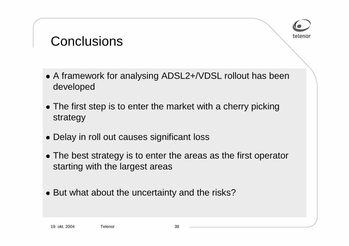
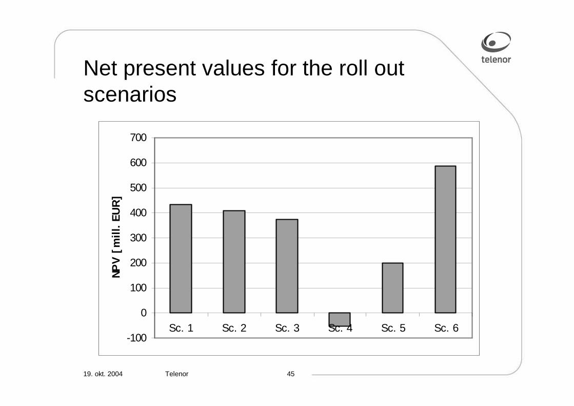
Conclusions
� A framework for analysing ADSL2+/VDSL rollout has been developed
� The first step is to enter the market with a cherry picking strategy
� Delay in roll out causes significant loss
� The best strategy is to enter the areas as the first operator starting with the largest areas
� But what about the uncertainty and the risks?

19. okt. 2004 Telenor 39
Risk analysis principles
0,68 0,74 0,80 0,86 0,92
Variable 1
Variable 2
1,09 1,54 2,00 2,46 2,91
Variable 3
0,55 0,78 1,00 1,23 1,45
Frequency Chart
kECU
,000
,007
,013
,020
,027
0
67,25
134,5
201,7
269
-3000 -1000 1000 3000 5000
10 000 Trials 52 OutliersNPV
Pro
bab
ility F
requen
cy
0,68 0,74 0,80 0,86 0,920,68 0,74 0,80 0,86 0,92
Variable 1
Variable 2
1,09 1,54 2,00 2,46 2,91
Variable 2
1,09 1,54 2,00 2,46 2,911,09 1,54 2,00 2,46 2,911,09 1,54 2,00 2,46 2,91
Variable 3
0,55 0,78 1,00 1,23 1,45
Variable 3
0,55 0,78 1,00 1,23 1,450,55 0,78 1,00 1,23 1,45
Frequency Chart
kECU
,000
,007
,013
,020
,027
0
67,25
134,5
201,7
269
-3000 -1000 1000 3000 5000
10 000 Trials 52 OutliersNPV
Pro
bab
ility F
requen
cy
Frequency Chart
kECU
,000
,007
,013
,020
,027
,000
,007
,013
,020
,027
0
67,25
134,5
201,7
269
0
67,25
134,5
201,7
269
-3000 -1000 1000 3000 5000-3000 -1000 1000 3000 5000
10 000 Trials 52 OutliersNPV
Pro
bab
ility F
requen
cy

19. okt. 2004 Telenor 40
Evaluation of the output distribution
Suppose Net Present Value is the output distribution
Alternative measures:
� Mean value
� Confidence interval
� 10% percentage
� 5% percentage
� Percentage of observations below NPV=0

19. okt. 2004 Telenor 41
Fitting of probability densities for the input variables
The probability densities have the ability not to give negative values.
The following input are convenient for defining the probability densities:
� Default value
� Minimum value
� 5% percentile
� 95% percentile
� Maximum value
19. okt. 2004 Telenor 42
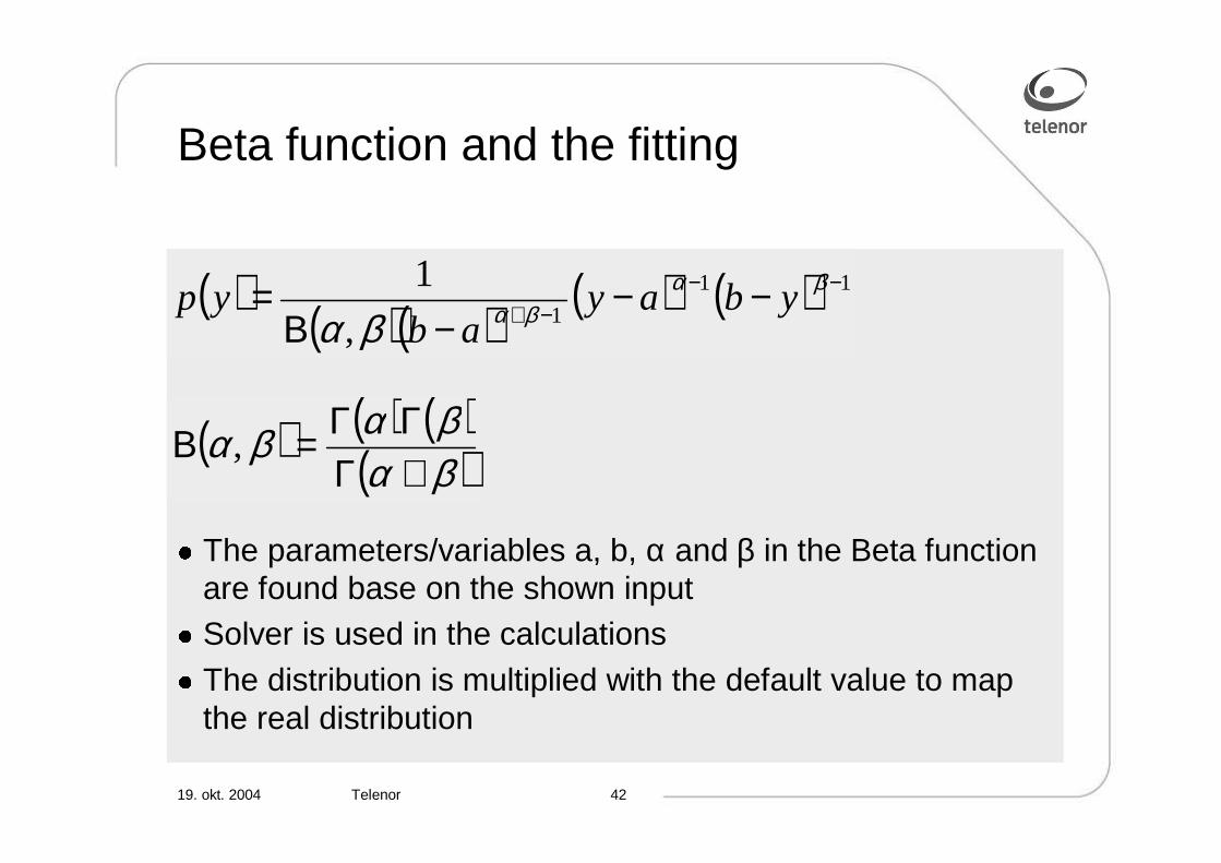
Beta function and the fitting
� The parameters/variables a, b, α and β in the Beta function are found base on the shown input
� Solver is used in the calculations
� The distribution is multiplied with the default value to map the real distribution
( ) ( )( ) ( ) ( ) 11
1,
1 −−−+ −−
−Β= βα
βαβαybay
abyp
( ) ( ) ( )( )βα
βαβα+ΓΓΓ=Β ,

19. okt. 2004 Telenor 43
Definition of probability functions for critical variables
Variable Name
Minimum Value
5% percentile
Default Value
95% percentile
Maximum Value
α β
Monthly ARPU 90 95 100 108 124.7 5.11 11.16
Line Card Price 1,200 1,400 1,600 1,800 2,000 4.94 4.94
Sales Costs 25% 27.5% 30% 32.5% 35% 4.94 4.94 Provisioning
Costs 50 60 65 70 80 11.77 11.77
Equipment Price
Reduction Rate
5% 8% 10% 12% 15% 8.02 8.02
Adoption Rate, final
year 26% 29% 32% 37% 42% 4.02 6.04
Customer Installations
Cost 100 110 120 130 140 4.95 4.95
Content Costs 50% 55% 60% 65% 70% 4.95 4.95 Smart Card
Costs 20 25 30 35 40 4.94 4.94
Customer Operations & Maintenance
15 20 25 30 35 4.95 4.95

19. okt. 2004 Telenor 44
TheThe business case business case approachapproach::
NPVNPV IRRIRR PaybackPeriod
PaybackPeriod
Economic Inputs
Cash flows, Profit & loss accounts
Geometric Model
Services Architectures
Year 0 Year 1 Year n Year m. . .
Demand for the Telecommunications Services
DB
RevenuesOA&MCosts
Life Cycle Cost
Life Cycle Cost
First Installed Cost
First Installed CostInvestments
Risk Assessment
19. okt. 2004 Telenor 45
Net present values for the roll out scenarios
-100
0
100
200
300
400
500
600
700
Sc. 1 Sc. 2 Sc. 3 Sc. 4 Sc. 5 Sc. 6
NP
V [
mil
l. E
UR
]

19. okt. 2004 Telenor 46
Net present value results from risk analysis. Different simulations
10 variables simulated Adoption rate and ARPU simulated
Only Adoption Rate simulated Scenario
5% perc. 95% perc. σ 5% perc.
95% perc. σ 5% perc.
95% perc. σ
Sc. 1 -48.5 1 155.7 364.1 -5.1 1 114.5 339.5 58.6 928.4 263.4
Sc. 2 -70.6 1 138.4 365.7 -27.4 1 097.3 341.2 37.6 909.7 265.6
Sc. 3 -102.3 1 108.3 366.4 -58.9 1 066.1 341.9 4.3 882.5 266.6
Sc. 4 -376.4 438.5 264.8 -341.4 408.4 227.6 -287.4 261.6 166.7
Sc. 5 -212.0 830.8 315.9 -174.2 795.8 293.8 -112.9 624.9 224.1
Sc. 6 -50.6 1 561.9 487.7 6.0 1 507.2 455.9 90.6 1 256.9 356.1
19. okt. 2004 Telenor 47
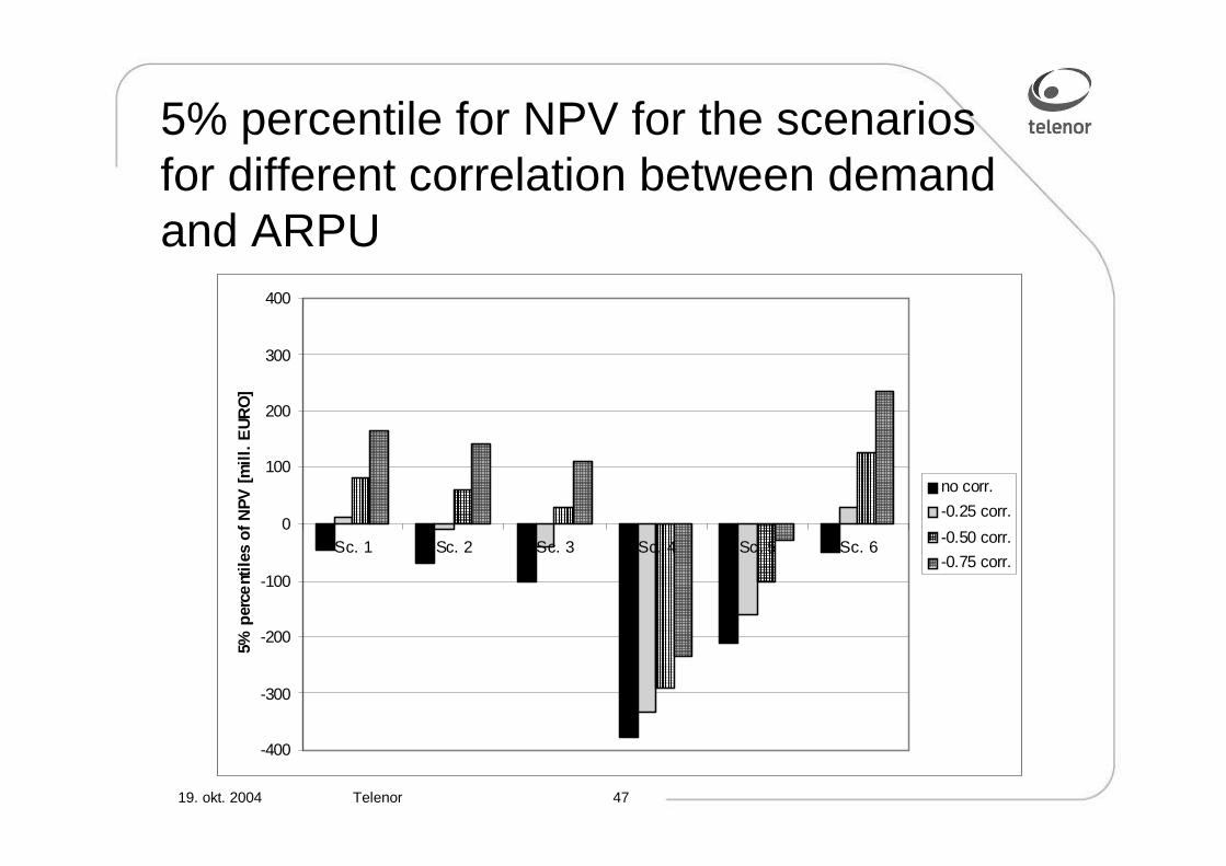
5% percentile for NPV for the scenarios for different correlation between demand and ARPU
-400
-300
-200
-100
0
100
200
300
400
Sc. 1 Sc. 2 Sc. 3 Sc. 4 Sc. 5 Sc. 6
5% p
erce
ntil
es o
f N
PV
[m
ill.
EU
RO
]
no corr.
-0.25 corr.
-0.50 corr.
-0.75 corr.

19. okt. 2004 Telenor 48
Conclusions
� The risk framework has been developed through the European programs RACE, ACTS and IST, by the projects RACE 2087/TITAN, AC 226/OPTIMUM, AC364/TERA and IST-2000-25172 TONIC.
� The presentation shows how risk analysis is applied on a specific business case for evaluation of the economic risks.
� The methodology for fitting the probability densities of critical variables in the business case is described
� The analysis also show the effect by modelling dependency between ARPU and demand in the risk simulations
