Forecasting Market Shares Using VAR and BVAR Models: A Comparison of their

Forecasting Performance

FRANCISCO F. R. RAMOS

Faculty of Economics, University of Porto, 4200 Porto, Portugal.E-mail: framos@fep.up.pt

2

Forecasting Market Shares Using VAR and BVAR Models: A Comparison of their

Forecasting Performance

This paper develops a Bayesian vector autoregressive model (BVAR) for the leader of the

Portuguese car market to forecast the market share. The model includes five marketing

decision variables. The Bayesian prior is selected on the basis of the accuracy of the out-

of-sample forecasts. We find that our BVAR models generally produce more accurate

forecasts of market share. The out-of-sample accuracy of the BVAR forecasts is also

compared with that of forecasts from an unrestricted VAR model and of benchmark

forecasts produced from univariate (e.g., Box-Jenkins ARIMA) models. Additionally,

competitive dynamics of the market place are revealed through variance decompositions

and impulse response analyses.

Classification system for journal articles: C110, C320, M310Key words: Automobile market; BVAR models; Forecast accuracy; Impulse responseanalysis; Marketing decision variables; Specification of marketing priors;Variancedecomposition; VAR models

3

INTRODUCTION

Multiple time series models have been proposed, for some time, as alternatives to

structural econometric models in economic forecasting applications. In the Marketing

field, applications of multiple time series models ( Transfer functions, Intervention and

VARMA models ) include for example Aaker, Carman and Jacobson (1982), Adams and

Moriarty (1981), Ashley, Granger and Schmalensee (1980), Bass and Pilon (1980),

Bhattacharyya (1982), Franses (1991), Grubb (1992), Hanssens (1980a, 1980b), Heyse

and Wei (1985), Heuts and Bronckers (1988), Jacobson and Nicosia (1981),

Krishnamurthi, Narayan and Raj (1986), Leone (1983, 1987), Lui (1987), Moriarty and

Salamon (1980), Moriarty (1985), Sturgess and Wheale (1985), Takada and Bass (1988),

and Umashankar and Ledolter (1983).

One class of multiple time series models which has received much attention

recently is the class of Vector Autoregressive (VAR) models. VAR models constitute a

special case of the more general class of Vector Autoregressive Moving Average

(VARMA) models. Although VAR models have been used primarily for macroeconomic

models, they offer an interesting alternative to either structural econometric (market share)

or univariate (e.g., Box-Jenkins ARIMA or exponential smoothing) models for problems

in which simultaneous forecasts are required for a collection of related microeconomic

variables, such as industry and firm sales forecasting. The use of VAR models for

economic forecasting was proposed by Sims (1980), motivated in part by questions related

to the validity of the way in which economic theory is used to provide a priori justification

for the inclusion of a restricted subset of variables in the "structural" specification of each

dependent variable 1. Sims (1980) questions the use of the so called "exclusionary and

identification restrictions". Such time series models have the appealing property that, in

order to forecast the endogenous variables in the system, the modeller is not required to

provide forecasts of exogenous explanatory variables; the explanatory variables in an

4

econometric model are typically no less difficult to forecast than the dependent variables.

In addition, the time series models are less costly to construct and to estimate. This does

not imply, however, that VAR models necessarily offer a parsimonious representation for

a multivariate process. While it is true that any stationary and invertible VARMA process

has an equivalent representation as a VAR process of possibly infinite order ( see, for

example, Fuller, 1976), it is usually the case that the VAR representation will not be as

parsimonious as the corresponding VARMA representation, which includes lags on the

error terms as well as on the variables themselves. Despite this lack of parsimony, and the

additional uncertainty imposed by the use of a finite-order VAR model as an

approximation to the infinite-order VAR representation, VAR models are of interest for

practical forecasting applications because of the relative simplicity of their model

identification and parameter estimation procedures, superior forecasting performance,

compared with those associated with structural and VARMA models 2. Brodie and De

Kluyver (1987) have reported empirical results in which simple "naive" market share

models (linear extrapolations of past market share values) have produced forecasts as

accurate as those derived from structural econometric market share models.

The number of parameters to be estimated may be very large in VAR models,

particularly in relation to the amount of data that is typically available for business

forecasting applications. This lack of parsimony may present serious problems when the

model is to be used in a forecasting application. Thus, the use of VAR models often

involves the choice of some method for imposing restrictions on the model parameters: the

restrictions help to reduce the number of parameters and / or to improve their estimability.

One such method, proposed by Litterman (1980), utilizes the imposition of stochastic

constraints, representing prior information, on the coefficients of the vector

autoregression. The resulting models are known as Bayesian Vector Autoregressive

(BVAR) models.

5

In this paper, we develop a Bayesian vector autoregressive model (BVAR) for the

leader of the Portuguese car market, for the period 1988:1 through 1993:6 using monthly

data. The rationale for the choice of a multiple time series technique is twofold. Structural

models of market share, as surveyed in Cooper and Nakanishi (1988), for example, tend to

be based on a number of generalizations about the effectiveness and relative importance of

advertising, price, and other elements of the marketing mix, with little emphasis being

placed on the correct determination of exogeneity assumptions and on the appropriate

dynamic model specification. Secondly, and presumably partly because of this, the

forecasting performance of such models has been poor compared to that of time series

models: for such evidence, see Brodie and De Kluyver (1987), Danaher and Brodie (1992)

and Brodie and Bonfrer (1994). Out-of-sample one-through twelve-months-ahead

forecasts are computed for the leader's market share and their accuracy is evaluated

relative to that of forecasts from an unrestricted VAR model and from best-fitting

univariate ARIMA models.

The paper is organized as follows. The next section briefly describes the VAR and

the BVAR modelling methodologies. The third section describes the data base used and

the rational behind the choice of the variables. The fourth section presents the forecasting

strategy, the main empirical results, and illustrate the use of impulse response analysis and

variance decompositions.We conclude with a section on the limitations of our research and

possible extensions.

VAR AND BVAR MODELLING

The theory underlying VAR models has its foundation in the analysis of the

covariance stationary linearly regular stochastic time series Yt . We assume here that Yt is

( )n ×1 in dimension, i.e., ′=Y Y Yt t nt( ,... )1 . By Wold's decomposition theorem Yt

possesses a unique one-sided vector moving-average representation which, assuming

6

invertibility, gives rise to an infinite-ordered vector autoregressive representation ( VAR).

In empirical work it is assumed that Yt can be approximated arbitrarily well by the finite

p-th ordered VAR :

Y B Y et k t k tk

p

= +−=

∑1

(1)

where et is a zero-mean vector of white noise processes with positive definite

contemporaneous covariance matrix and zero covariance matrices at all other lags; and the

Bk 's are ( )n n× coefficient matrices with elements bijk . This approximation assumption

holds, in fact, if Yt is covariance-stationary linearly-regular process. Equation (1) can be

used to generate the forecast f t h, at time t of Yt h+ , with subsequent forecast error

e Y ft h t h t h, ,= −+ and error variance-covariance matrix V E(e e )h t,h t ,h= ⋅ ′ . Granger and

Newbold (1986, ch. 7 ) show that the optimal ( in terms of minimizing the quadratic form

associated with Vh ) h period ahead forecast f t h, of Yt h+ made at time t is

f B ft h k t h kk

p

, ,= −=

∑1

(2)

where f Yt h k t k h, ( )− − −= for k h h p= +, ,...,1 , and Bk 's are the coefficient matrices in

equation (1).

Equation (1) is the prototype for all of the variations of VAR 's mentioned

hereafter.The several approaches differ primarily in terms of one or more of the following

considerations: (1) transformation of the data and the inclusion of non-random

deterministic variables; (2) determination of the maximum lag length p ; (3) specification

of non-zero elements of the coefficient matrices Bk , k p= 1,... ; (4) estimation of the

coefficients. We will now briefly describe each approach and highlight its distinguishing

features.

7

The unrestricted VAR

In a VAR with n variables there is an individual equation for each variable. For the

unrestricted case there are p lags for each variable in each equation. For example, the

equation for the ith variable is

Y b Y b Y eit i k t kk

p

ink n t kk

p

it= + + +−=

−=

∑ ∑1 11 1

, ,... . (3)

As in the problem of seemingly unrelated regressions, when the right-hand-side variables

are the same in all equations the applications of OLS equation by equation is justified. The

coefficient estimates are maximum likelihood estimates conditioned on the initial

observations, and under a variety of alternative assumptions on the Y 's and e 's , are

consistent, asymptotically efficient, and asymptotically normally distributed ( Litterman,

1980 ). The unrestricted VAR has been used extensively by Sims (1980), and in the initial

stages of the model building by Caines, Keng and Sethi (1981), Tiao and Box (1981), and

Tiao and Tsay (1983).

In terms of data transformations, Tiao and Box (1981), and Tiao and Tsay (1983)

recommend against differencing each individual series to achieve stationarity. Acording to

Tiao and Tsay, differencing is not only unnecessary when considering several series jointly,

but will lead to unnecessary complexity in the model. Neither Tiao and Box nor Tiao and

Tsay make recommendations on the use of instantaneous data transformations or

deterministic trend components. In empirical work they log the data but do not include

time trends. Maximum lag length is determined in each case by using a slight variation of

the likelihood ratio statistic and testing the null hypothesis that Bk = 0 for sucessive lag

lengths.

8

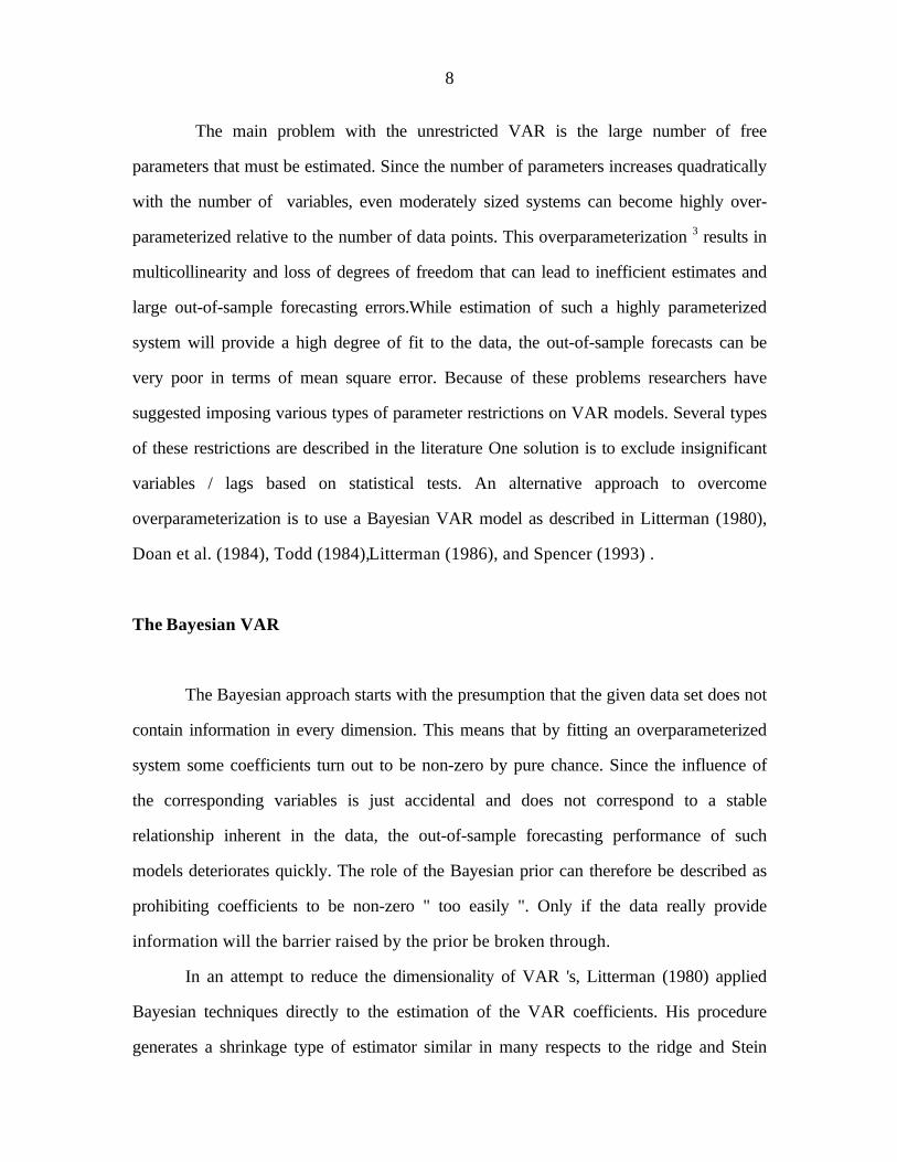
The main problem with the unrestricted VAR is the large number of free

parameters that must be estimated. Since the number of parameters increases quadratically

with the number of variables, even moderately sized systems can become highly over-

parameterized relative to the number of data points. This overparameterization 3 results in

multicollinearity and loss of degrees of freedom that can lead to inefficient estimates and

large out-of-sample forecasting errors.While estimation of such a highly parameterized

system will provide a high degree of fit to the data, the out-of-sample forecasts can be

very poor in terms of mean square error. Because of these problems researchers have

suggested imposing various types of parameter restrictions on VAR models. Several types

of these restrictions are described in the literature One solution is to exclude insignificant

variables / lags based on statistical tests. An alternative approach to overcome

overparameterization is to use a Bayesian VAR model as described in Litterman (1980),

Doan et al. (1984), Todd (1984), Litterman (1986), and Spencer (1993) .

The Bayesian VAR

The Bayesian approach starts with the presumption that the given data set does not

contain information in every dimension. This means that by fitting an overparameterized

system some coefficients turn out to be non-zero by pure chance. Since the influence of

the corresponding variables is just accidental and does not correspond to a stable

relationship inherent in the data, the out-of-sample forecasting performance of such

models deteriorates quickly. The role of the Bayesian prior can therefore be described as

prohibiting coefficients to be non-zero " too easily ". Only if the data really provide

information will the barrier raised by the prior be broken through.

In an attempt to reduce the dimensionality of VAR 's, Litterman (1980) applied

Bayesian techniques directly to the estimation of the VAR coefficients. His procedure

generates a shrinkage type of estimator similar in many respects to the ridge and Stein

9

estimators. Since there is a ridge regression analogy to the BVAR, it is not surprising that

BVAR solved the multicollinearity problem. As is well known, from a Bayesian standpoint

shrinkage estimators can be generated as the posterior means associated with certain prior

distributions. While Litterman 's estimator can be justified as a posterior mean, the

economic content of the prior information is not strong. Litterman's prior gives us a

middle ground between the extremes of usual structural specification (strong unbelievable

priors) and unrestricted VARs (no priors).

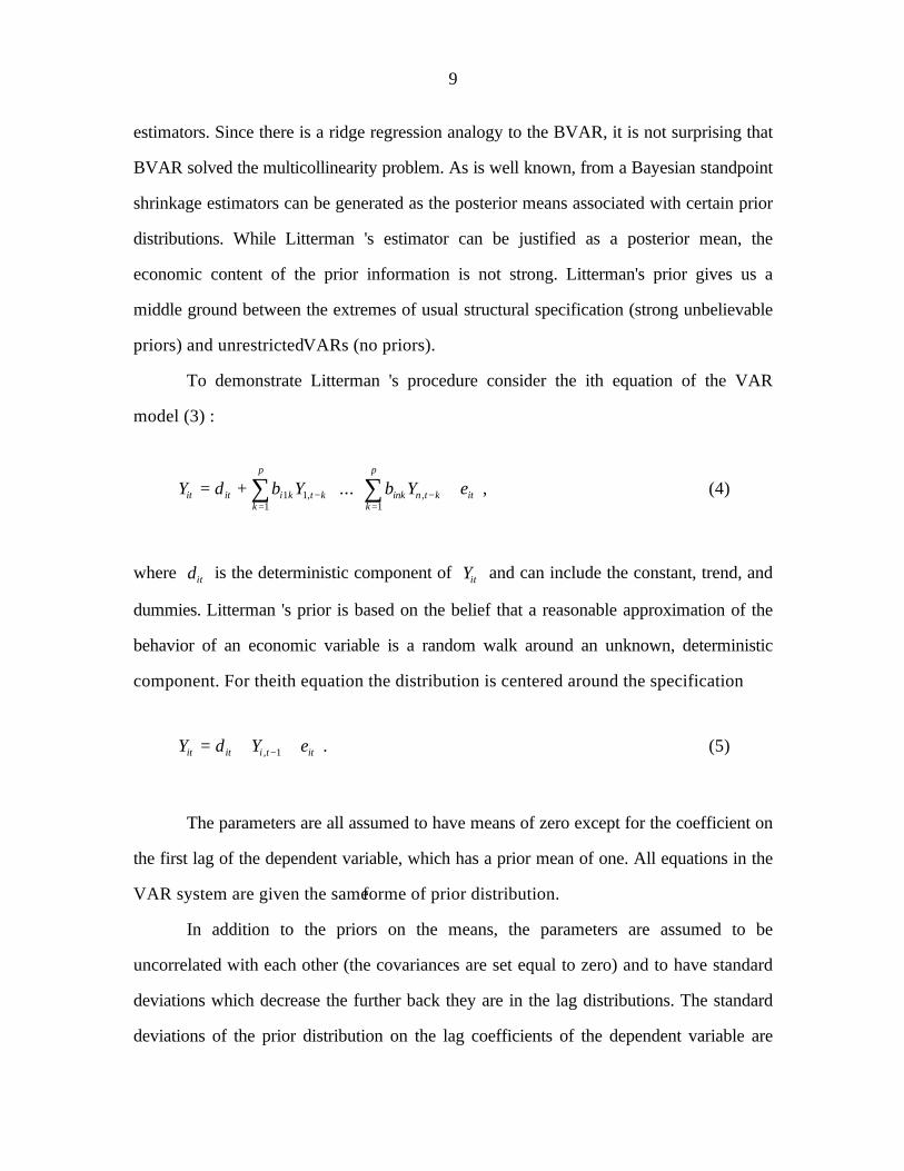
To demonstrate Litterman 's procedure consider the ith equation of the VAR

model (3) :

Y d b Y b Y eit it i k t kk

p

ink n t kk

p

it= + + +−=

−=

∑ ∑+ 1 11 1

, ,... , (4)

where dit is the deterministic component of Yit and can include the constant, trend, and

dummies. Litterman 's prior is based on the belief that a reasonable approximation of the

behavior of an economic variable is a random walk around an unknown, deterministic

component. For the ith equation the distribution is centered around the specification

Y d Y eit it i t it= + +−, 1 . (5)

The parameters are all assumed to have means of zero except for the coefficient on

the first lag of the dependent variable, which has a prior mean of one. All equations in the

VAR system are given the same forme of prior distribution.

In addition to the priors on the means, the parameters are assumed to be

uncorrelated with each other (the covariances are set equal to zero) and to have standard

deviations which decrease the further back they are in the lag distributions. The standard

deviations of the prior distribution on the lag coefficients of the dependent variable are

10

allowed to be larger than for the lag coefficients of the other variables in the system. Also,

since little is known about the distribution of the deterministic components, a "flat" or

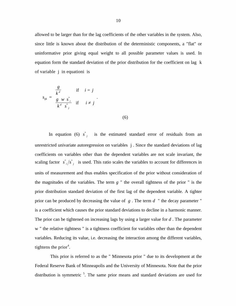
uninformative prior giving equal weight to all possible parameter values is used. In

equation form the standard deviation of the prior distribution for the coefficient on lag k

of variable j in equation i is

s

gk

i j

g wk

i jijk

d

id

j

==

⋅ ⋅⋅

≠

if

if σ

σ

.

(6)

In equation (6) σ j is the estimated standard error of residuals from an

unrestricted univariate autoregression on variables j . Since the standard deviations of lag

coefficients on variables other than the dependent variables are not scale invariant, the

scaling factor σ σi j is used. This ratio scales the variables to account for differences in

units of measurement and thus enables specification of the prior without consideration of

the magnitudes of the variables. The term g " the overall tightness of the prior " is the

prior distribution standard deviation of the first lag of the dependent variable. A tighter

prior can be produced by decreasing the value of g . The term d " the decay parameter "

is a coefficient which causes the prior standard deviations to decline in a harmonic manner.

The prior can be tightened on increasing lags by using a larger value for d . The parameter

w " the relative tightness " is a tightness coefficient for variables other than the dependent

variables. Reducing its value, i.e. decreasing the interaction among the different variables,

tightens the prior 4.

This prior is referred to as the " Minnesota prior " due to its development at the

Federal Reserve Bank of Minneapolis and the University of Minnesota. Note that the prior

distribution is symmetric 5. The same prior means and standard deviations are used for

11

each independent variable in each equation and across equations, and the same priors are

used for each dependent variable across equations.

The BVAR model is estimated using Theil 's (1971) mixed-estimation technique

that involves supplementing data with prior information on the distributions of the

coefficients. For each restriction on the parameter estimates, the number of observations

and degrees of freedom are increased by one in an artificial way. The loss of degrees of

freedom due to overparameterization associated with a VAR model is therefore not a

problem with the BVAR model. The incorporation of the prior information in the

estimation of the ith equation is accomplished by re-writing equation (4) as

Y XB ei i i= + (7)

where Yi is the vector of observations on Yit ; X is the matrix of deterministic

components and observations on all lags of variables; Bi is the vector of coefficients on

deterministic components and lags of variables; and ei is the ( )T ×1 residual vector. The

estimator suggested by Litterman is

( ) ( )B X X h R R X Y h R ri i i i i i i i= ′ + ′ ′ + ′−1

(8)

where Ri is a diagonal matrix with zeros corresponding to the deterministic components

and elements ( )g sijk corresponding to the kth lag of variable j , j = 1,...n ; ri is a vector

of zeros and a one corresponding to the first lag of the dependent variable i ; and

h gi i= σ 2 2 . Bi is immediately seen to be a version of Theil 's mixed estimator where

R B r vi i i i= + and vi is distributed ( )N g I0 2, .

To apply Litterman 's procedure one must search over the parameters g, d, and w

until some predetermined objective function is optimized. The objective function can be

12

the out-of-sample mean-squared forecast error, or some other measure of forecast

accuracy. Doan, Litterman and Sims (1984) suggest minimizing the log determinant of the

sample covariance matrix of the one-step-ahead forecast errors for all the equations of the

BVAR. In a forecasting comparison such as ours, a portion of the sample must be

withheld to determine the parameters g, d, and w ; while the remainder of the sample is

used with the selected model to generate out-of-sample forecasting statistics for

comparison purposes.

DATA

The data base used for this study is a monthly time series sample of market share,

and 5 marketing variables, for the period 1988:1-1993:6 in the car market in the Portugal.

The marketing variables include such variables as relative price, major media advertising

expenditures ( TV, radio,and newspaper), and an Age variable for the leader brand in the

car market. The portuguese car market consists of twenty five imported car brands, but

the top six account on average for 82.3% of the total market, with a standard deviation of

4.75%. The leader is a general brand, presented in all segments of the market and

represents on average 16.8% of the total market, with a standard deviation of 3.56%.

The time series variables used in this study are defined as following:

MS t1 = market share of the leader brand,

A t1 = relative age of the leader brand,

P t1 = relative price of the leader brand,

TVS t1 = TV advertising expenditures in shares of the leader brand,

RS t1 = Radio advertising expenditures in shares of the leader brand, and

PS t1 = Press(newspaper and magazine) advertising expenditures in shares of the

leader brand.

13

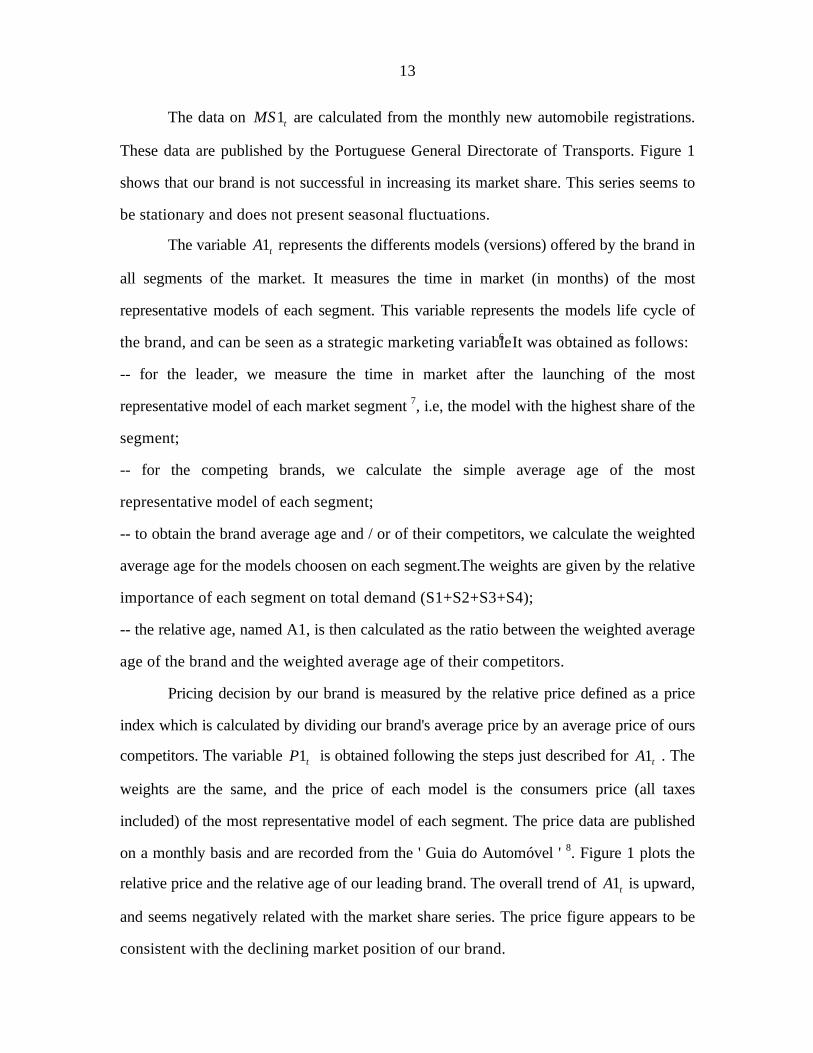
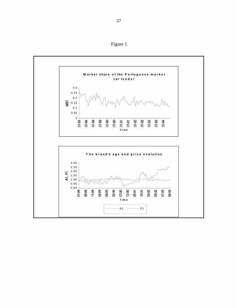
The data on MS t1 are calculated from the monthly new automobile registrations.

These data are published by the Portuguese General Directorate of Transports. Figure 1

shows that our brand is not successful in increasing its market share. This series seems to

be stationary and does not present seasonal fluctuations.

The variable A t1 represents the differents models (versions) offered by the brand in

all segments of the market. It measures the time in market (in months) of the most

representative models of each segment. This variable represents the models life cycle of

the brand, and can be seen as a strategic marketing variable 6. It was obtained as follows:

-- for the leader, we measure the time in market after the launching of the most

representative model of each market segment 7, i.e, the model with the highest share of the

segment;

-- for the competing brands, we calculate the simple average age of the most

representative model of each segment;

-- to obtain the brand average age and / or of their competitors, we calculate the weighted

average age for the models choosen on each segment.The weights are given by the relative

importance of each segment on total demand (S1+S2+S3+S4);

-- the relative age, named A1, is then calculated as the ratio between the weighted average

age of the brand and the weighted average age of their competitors.

Pricing decision by our brand is measured by the relative price defined as a price

index which is calculated by dividing our brand's average price by an average price of ours

competitors. The variable P t1 is obtained following the steps just described for A t1 . The

weights are the same, and the price of each model is the consumers price (all taxes

included) of the most representative model of each segment. The price data are published

on a monthly basis and are recorded from the ' Guia do Automóvel ' 8. Figure 1 plots the

relative price and the relative age of our leading brand. The overall trend of A t1 is upward,

and seems negatively related with the market share series. The price figure appears to be

consistent with the declining market position of our brand.

14

The data on TVS t1 , RS t1 , and PS t1 are expressed as shares of total advertising

expenditures by media (us industry) and were obtained from ' Sabatina ' 9. Figure 1

indicates that major media advertising has been used extensively by our brand, and has

fluctuated widely over the observed time period.

A preliminary examination suggested that these variables are all stationary 10. This

dataset is available from the author on request.

( Figure 1 about here )

EMPIRICAL APPLICATION

Models selected

Three classes of models are included in our empirical comparisons 11, each class

being represented by one or more specific models. The classes are univariate Box-Jenkins,

unrestricted VAR, and BVAR. The usual criteria, e.g. stationarity, autocorrelation, and

partial autocorrelation functions, significance of coefficients, and the Akaike Information

Criterion, are used to select the best models.

All variables are measured in logs to handle nonstationarity in variance, i.e.,

heteroscedasticity.

The best-fit ARIMA model for MS1 is as follows:

( . ) . ( . )

( . ) ( . ) ( . )

1 0 916 1 1 898 1 0 814

0 03 0 06 0 07

− = − + +B MS B et t

a a a ,

standard errors are in parentheses and a means significant at the 0.01 level. As

Montgomery and Weatherby (1980, p. 306) note: ' The Box-Jenkins approach uses

15

inefficient estimates of impulse reponses weights which are matched against a set of

anticipated patterns, implying certain choices of the parameters ... the analyst's skill and

experience often play a major role in the success of the model building effort '. 12

To determine the optimal lag length of the unrestricted VAR [ VAR(U) ] we have

employed the likelihood ratio test statistic ( LR ), suggested by Sims(1980) 13. Given the

number of observations, we have considered a maximum lag of nine and then tested

downwards. The LR test supports the choice of six lags. Our six-variable VAR system

with a lag length of 6 and 37 parameters (including the constant) in each equation, was

then efficiently estimated in levels (so that it is comparable to the BVAR model), using

least squares estimators 14. A summary of these estimation results is provided by the

critical levels of F-tests of the hypothesis that all lags of a particular variable in each

equation are zero. These critical levels are reported in table 1. An examination of table 1

immediately reveals that the relative age of our brand ( A1) has a significant effect on

MS1, P1 and TVS1. There is some indication that relative age movements precede those

on market share, relative price and TV advertising expenditures. TV advertising

expenditutes has seen to have a significant effect not just on market share, which is

perfectly predicted by the marketing theory of advertising effects on sales, but also on

press advertising expenditures (PS1). This later relation means that there is evidence

relating the Press advertising expenditures with TV actions.

( Table 1 about here )

In the class of BVAR models, the variables are specified in levels because as

pointed out by Sims et al. (1990, p. 360) ' ... the Bayesian approach is entirely based on

the likelihood function, which has the same Gaussian shape regardless of the presence of

nonstationarity, [hence] Bayesian inference need take no special account of nonstationarity

' 15 . The models are estimated with six lags on each variable 16.

16

The 'optimal' Bayesian prior was selected by minimising, for the period 1992:1 to

1992:12, the RMSEs statistics for one-to six-months-ahead forecasts. In a first step we

assume a symmetric prior, i.e., f i j w i j( , ) ,= ≠ [ BVAR(S) ], then we relax this

assumption to take in account a more general interaction between the variables

[BVAR(G)] (see footnote 5).

Specification of Marketing priors

In our search for the symmetric prior we have considered three values for w :

0.25, 05, 075. For example, w = 0.5 means that, in the market share equation of our

BVAR system, all right-hand-side variables, except the lagged market share, enter with a

weight of 50%. For the parameter g we have assumed a relatively ' loose ' value of 0.3

and a 'tight ' value of 0.1. We set the harmonic lag decay, d , to 1 as recommended by

Doan, Litterman and Sims (1984) . This has given us six alternative specifications. The

best values according to our criterion function 17 were obtained for g = 0.3, w = 0.5 and d

= 1 .

As an alternative to the symmetric prior, general tightness parameters are specified

equation-by-equation. This means that ours prior beliefs, based on marketing theory and /

or management experience, could be incorporated in a more precisely way. To specify the

general prior we have to define g , d , and the inter-series tightness parameters , f i j( , ) .

The initial values of overall tightness, g , and harmonic lag decay, d , are set at 0.2 and 1,

respectively. These are recommended in Doan (1992). The initial values for f i j( , ) , the

relative weights of variable j in equation i, are set from the information provided by table

1, marketing theory and author's beliefs. The BVAR model is initially estimated with these

parameters and the average of the RMSEs for one to six months ahead is recorded for

each variable for the period 1992:1 to 1992:12. The parameters in the prior are changed

17

sequentially and after some initial search, the best values were obtained for d = 1, g = 0.15

and

f i j

eq v MS A P TVS RS PS

MS

A

P

TVS

RS

PS

( , )

.. . . . .

. . . . .

. . . . .

. . . . .

. . . . .

. . . . .

=

. 1 1 1 1 1 1

1

1

1

1

1

1

1 8 5 4 1 15 1 1 1 1 15 5 1 1 1 14 5 1 1 1 14 1 1 4 1 14 1 1 5 1 1

.

The tightness parameters represent the authors' subjective priors on the tightness

of the coefficients associated with lagged values of variables listed in the right-hand

columns. Of course, these priors do not represent much more than a single person's

opinion and are certainly not thought to reflect substantive opinion--which of course

would be an interesting extension. Substantive experts (subject matter experts) may

possess prior information on the center of the distribution of coefficients on lagged

variables as well. While this information may prove difficult to elicit, the potential for

forecasting improvement makes further work along this line important.

Evaluation of accuracy

The accuracy of the out-of-sample forecasts for 1993:1 to 1994:6 is measured by

the RMSE and the Theil U statistics for one-to twelve-months-ahead forecasts. If At

denotes the actual value of a variable, and Ft the forecast made in period t , then the

RMSE and the Theil statistic are defined as follows:

( )RMSE A F N

U RMSE RMSE

t j k t j kj

k

= −

=

+ + + +=

∑2

1

0 5

/

( ) / ( )

.

model random walk

18

where k = 1 2 12, ,... denotes the forecast step and N is the total number of forecasts in the

prediction period.

The U statistic is the ratio of the RMSE for the estimated model to the RMSE of

the simple random walk model which predicts that the forecast simply equals the most

recent information. Hence if U < 1, the model performs better than the random walk

model without drift; if U > 1, the random walk outperforms the model. The U statistic is

therefore a relative measure of accuracy and is unit-free (Bliemel, 1973). The forecasted

value used in the computation of the RMSE and U statistics is the level (in logarithm) of

the market share, so these statistics can be compared across the different models.

The RMSE and the U statistics are generated using the Kalman filter algorithm in

RATS. The models are estimated for the initial period 1988:1 to 1992:12. Forecasts for up

to twelve months ahead are computed. One more observation is added to the sample and

forecasts up to twelve months ahead are again generated and so on. Based on the out-of-

sample forecasts, RMSEs and the Theil U statistics are computed for one-to twelve-

months-ahead forecasts. The relevant comparison is on "out-of-sample" forecasts.

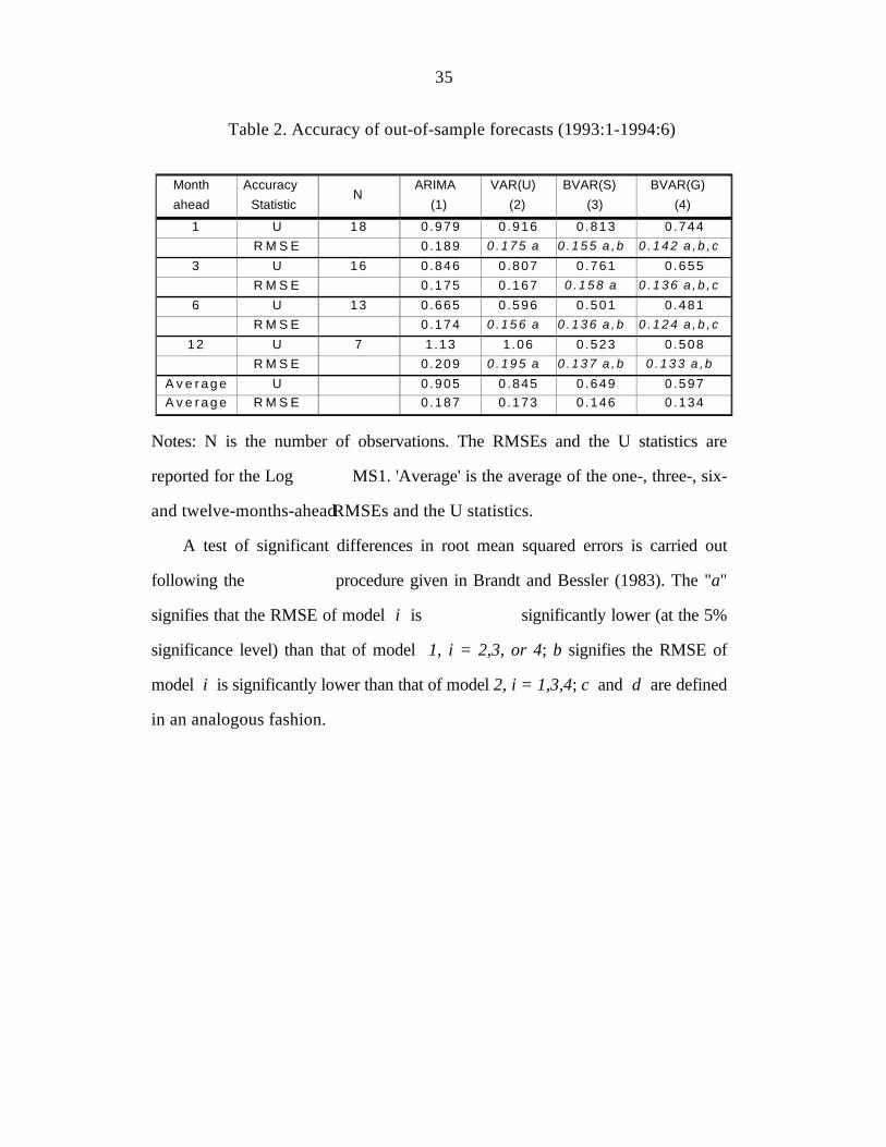
The RMSEs and the U statistics for MS1 for the four models discussed above are

reported in table 2. The table also reports the average of the RMSEs and of the U

statistics for the one-,three-,six- and twelve-months-ahead forecasts, and summaries of

tests of significant differences among the RMSEs mesures. The conclusions from table 2

are as follows:

(1) RMSEs versus Theil U statistics: The RMSEs and the Theil U statistics do not

follow a consistent pattern with an increase in the forecast horizon.

(2) BVAR versus univariate ARIMA models: BVAR models produce more accurate

forecasts (for all horizons) than the corresponding ARIMA model 18.

19

(3) BVAR versus the unrestricted VAR models: In all cases, BVAR(G) outperforms

the unrestricted VAR model. The comparison between BVAR(S) and VAR(U) produces

the same conclusion; BVARs are always superior for all forecasting periods.

(4) BVAR(G) versus BVAR(S): BVAR(G) offers the best out-of-sample forecast

performance, except at lag twelve where its RMSEs (U's) are not significantly lower than

those of the symmetric prior. Without regard to significance, the general prior yields the

lowest RMSEs (U's). This is not surprising since the prior for the model was selected on

the basis of minimisation of the average of one-to six-month-ahead RMSEs.

The results, in general, show that there are gains from using a BVAR approach to

forecasting. BVAR models produce more accurate forecasts than the alternative forecasts.

Finally, like other authors (Hafer and Sheehan, 1989) we found that the accuracy

of the forecasts is sensitive to the specification of the priors. If the prior is not well

specified, an alternate model such as an unrestricted VAR or an ARIMA model may

perform better.

( Table 2 about here )

Performance of alternative models in predicting turning points

While the BVAR models, in general, produce the most accurate forecasts, another

way to evaluate the performance of alternative models is to examine their ability in

predicting turning points, which are of key managerial significance. This topic is of vital

importance, as statistical methods can perform extremely well in terms of forecasting

overall levels, and yet still perform poorly in the prediction of turning points.

Unfortunately, the question of turning points does not easily lend itself to quantitative

analysis due to difficulties in, firstly, defining turning points; and, secondly, knowing when

20

a given method has adequately predicted a turn. Moreover, there are various types of turn

(e.g., those which are seasonal, cyclical, due to saturations in trends, etc.) which need to

be dealt with.

We focus on the performance of the BVAR models relative to that of the

unrestricted VAR and the univariate ARIMA models. Figure 2 shows that, in spite of the

unrestricted VAR model generally correctly predict the direction of change, BVAR

models are superior and do very well in predicting turning points. As such, BVAR models

can be recognized as important to the planning function in the organization. As the growth

in the formalization of the budgeting process continues, the strategic role of accurate

forecasting methods as the 'budget cornerstone' will continue to be emphasized (

Dalrymple, 1987).

(Figure 2 about here)

Besides generating excellent baseline forecasts, BVAR models can also be used to

study the effects of movements in one variable on movements in others using impulse

response analysis and variance decompositions.

Impulse response analysis

Impulse responses are the time paths of one or more variables as a function of a

one-time shock to a given variable or set of variables. Impulse responses are the dynamic

equivalent of elasticities. For example, in a static multiplicative interaction model of the

form ms p= ⋅α β price elasticity ε β= =( / )( / )dms dp p ms is constant. However, in a

dynamic system, changes in market share in one month are a function of changes in price

over several months. The net effect must be represented as a convolution sum. The

graphic representation of this sum provides a complete description of the dynamic

21

structure of the model ( it is incorrect to directly interpret estimated coefficients for the

variables of a BVAR model).

To illustrate, figure 3a shows the impulse responses of MS1 to a shock to each one

of the five marketing variables of the system. The results show that over the sample period

an unexpected increase in A1 produces a longer decrease (over 6 months) of MS1 that is

not totally recuperated after 12 months, i.e., A1 has a negative permanent impact on MS1.

The MS1 responses to shocks on advertising expenditures (TV, Radio and Press) are

positive, lagged and varying in magnitude. TV advertising effects begin after 3 months, but

seems to rest for a period longer than that of Radio and Press. Our findings are consistent

with the theory of the cumulative advertising effects on sales (e.g., Palda, 1964) and, even

the measurement and duration ["the p implied duration interval" in Clarke's (1976)

terminology] of these effects are easy to calculate. Surprisingly, the response of the MS1

to a price shock does not appear to be significant. A plausible explanation for this behavior

is that our brand does not compete on a price basis and even if it charges its prices, these

increases will be associated with the lauching of new models (versions).

The responses of A1 to a positive shock on MS1 and on P1 are given in Fig. 3b.

The results show that an unexpected increase in market share or on prices generates a fast

decrease on A1. Positive shocks on sales or on prices would probably stimulate the

introduction of new models in market (A1 decrease).

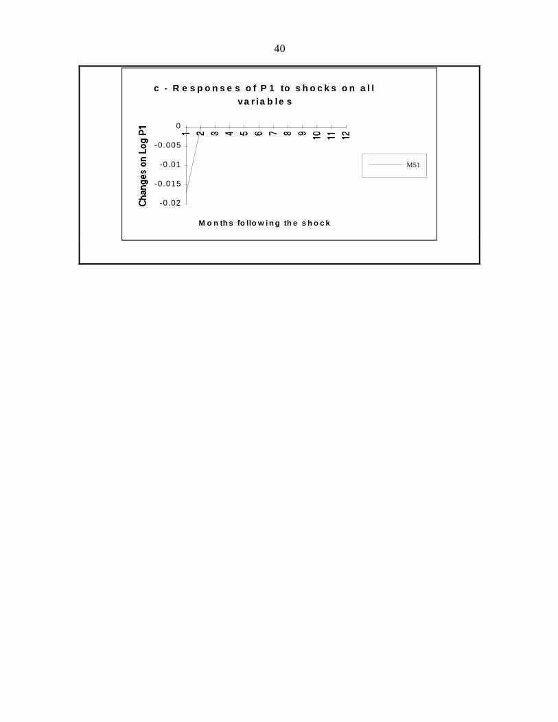
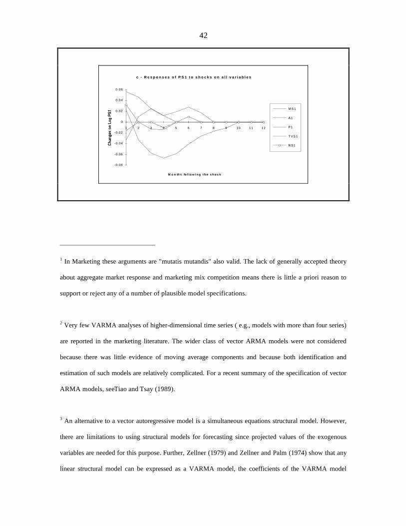
Fig 3c shows that prices react negatively to an increase in market share. This result

is spurious and does not make any sense in light of marketing theory.

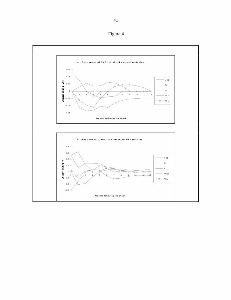
Figure 4 (a, b, c) show that all three advertising variables react positively (increase

its shares) to an unexpected increase in market share. However, the impact is more

important in Radio advertising expeditures than in the others. Our findings confirm the

existence of a feedback relationship between sales (market share) and advertising

expenditures.

22

The effect of interaction among the advertising variables is one of the issues that

deserves to be investigated in this analysis. For example, while an increase in TV

advertising is followed one month later by increases in Radio and Press advertising

expenditures, reenforcing the major role of TV advertising, an increase in Press advertising

seems to produce an opposite reaction. The impact of RS1 on TVS1 and PS1 does not

appear to be significant in either direction. We show evidence that confirm the existence of

interactions between the advertising variables and that the nature of these interactions vary

accordingly with the variable that produced the reaction.

(Figure 3 about here)

(Figure 4 about here)

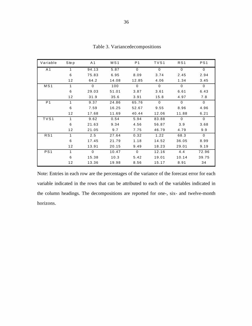
Variance decompositions

Variance decompositions give the proportion of the h-periods-ahead forecast error

variance of a variable that can be attributed to another variable. The pattern of the

variance decomposition also indicates the nature of Granger causality among the variables

in the system, and as such, can be very valuable in making at least a limited transition from

forecasting to understanding. If innovations in A t1 result in unexpected fluctuations in

MS t1 , then information on A t1 would be useful in predicting MS t1 . In interpreting these

variance decompositions, one should bear in mind Runkle's (1987) criticism that the

implicit confidence intervals attached to both variance decompositions and impulse

responses functions are often so large as to render precise inferences impossible.

The Choleski decompositions are examined for the BVAR(G) model. The variables

are ordered in the following sequence - A MS P TVS RS PSt t t t t t1 1 1 1 1 1, , , , , . This ordering

is based partly on our prior belief that changes in A t1 promote a response in MS t1 and

P t1 , which then, through the created expectations, alters TVS RS PSt t t1 1 1, , , and partly

23

on the timing of the availability of data to management. For instance, information on prices

and market shares is released before that on advertising expenditures 19.

The variance decompositions for our six variables model for the period 1988:1 to

1993:6 are reported in table 3. For each variable in the left-hand column, the percentage of

the forecast error variance for one, six and twelve months ahead that can be attributed to

shocks in each of the variables in the remaining columns is reported. Each row sums to

100% (ignoring rounding errors) since all the forecast error variance in a variable must be

explained by the variables in the model. If a variable is exogenous in the Granger sense,

i.e. if other variables in the model are not useful in predicting it, a large proportion of that

variable's error variance should be explained by its own innovations. How large is 'large'?

According to Doan (1992), in a six-variable model such as ours, 50% is quite high. If

another variable is useful in explaining a left-column variable, that useful variable will

explain a positive percentage of the prediction error variance. In practice, it is difficult to

distinguish between a variable that has no predictive value and one that has little predictive

value. Some conclusions, however, can be derived by comparing the magnitudes.

Table 3 shows that at a forecast horizon of 12 months, only 35.6% of the forecast

error variance in the MS1 is explained by its own innovations supporting the assumption

that MS1 is not exogenous, and other variables like A1, TVS1, and PS1 can be equally

useful in forecasting MS1. Market share is extremely stable from one month to the next --

none of the other variables figure at all in its 1-month ahead forecast. Moreover, longer

term forecasts of market share are heavily influenced by "age", TV advertising and not

much at all by price. The exogenous behaviour of A1 seems to be reflected in the 64.2%

error variance explained by its own innovations. The results for the price variable vary

with the horizon of forecasting. For instance, the market share variable seems more

important at shorter horizons (1 to 6), while the "age" variable becomes the largest

contributor for longer horizons (12 months).

24

There are some interesting media differences in the advertising variable. TV

advertising seems much more "exogenous" than the other media advertising (46.79% vs.

29.01% and 34%). Long term forecasts of TV advertising are rather more explained by

innovations in A1 than on MS1. However, for RS1 and PS1 it is the MS1 innovations

which help explain most of the forecast error variance attributable to other innovations.

(Table 3 about here)

LIMITATIONS AND EXTENSIONS

In this paper, we demonstrate the utility of VAR and BVAR methodologies as a

marketing tool that fulfils two requirements: it forecasts market share, and it provides

insights about the competitive dynamics of the marketplace. Here are compared the

forecasting accuracy of BVAR with several traditional approaches. Using data, we

establish that BVAR is a superior forecasting tool compared to univariate ARIMA and

VAR models. Because BVAR uses few degrees of freedom and is easy to identify, it

satisfies the practical requirements as a marketing forecasting tool. Finally, using impulse

response functions and variance decompositions, we illustrate that BVAR provides

important insights for the marketing manager.

Although BVAR is a promising and reliable forecasting tool, certain limitations

should be pointed out. First, BVAR models are highly reduced forms. Structural

interpretations based on the signs and magnitudes of estimated parameters should be

avoided. Hypothesis about effects should be tested using impulse response analysis.

Second, the accuracy of the forecasts is sensitive to the specification of the prior. If

the prior is not well specified, an alternate model such as an unrestricted VAR or an

ARIMA model may perform better. Third, the prior that is selected on the basis of some

25

objective function ( e.g. the Theil's U ) for the out-of-sample forecasts may not be

"optimal " for beyond the period for which it was selected.

This model, like all time series models, is best suited for stable environments ( e.g.

wide-sense stationary processes) where sufficient number of observations are available.

Thus, BVAR is not a new product model and its forecasts may be unreliable in markets

characterized by frequent new entries or drop-outs.

We propose several extensions of this initial application of BVAR to forecast

brand market shares. First, the bayesian approach can be improved by putting more

structure based on marketing theory into the prior thereby abandoning the symmetric

treatment of all variables. This would make the approach more bayesian in spirit since the

prior can now reflect better the a priori beliefs of the investigator. On the other hand the

greater flexibility makes it more difficult to find the optimal forecasting model. Second, the

inclusion of the contemporaneous values of some variables in some equations (using, e. g.,

a Wold causal ordering) may result in improved forecasting accuracy due to a simpler

model specification. Third, we used one specification of each model to forecast over the

entire testing period. More frequent specifications ( e.g., a time-varying parameter BVAR

model) would no doubt improve accuracy. An important problem deals with how often a

model should be reespecified. Finally, we used single equation procedures to estimate all

models. Forecasting accuracy may improve by estimating all equations in each model

simultaneously and exploiting the information in the cross-equation residual covariance

matrix.

Our experience with BVAR models suggests that it is a robust, reliable marketing

forecasting tool.

26

Footnotes:

27

References:

Aaker, David , James Carman and Robert Jacobson (1982), " Modeling Advertising-Sales

relationships involving feedback: A Time series analysis of six cereal brands," Journal of

Marketing Research, 19 (February), 116-125.

Adams, Arthur and Mark Moriarty (1981), " The advertising-sales relationship: Insights

from Transfer-function modeling," Journal of Advertising Research, 21 (June), 41-46.

Ashley, R., Clive Granger and Richard Schmalensee (1980), "Advertising and Aggregate

Consumption: An analysis of causality," Econometrica, 48 (July), 1149-1167.

Bass, Frank and Thomas Pilon (1980), "A stochastic brand choice framework for

econometric modeling of time series market share behavior," Journal of Marketing

Research, 17 (November), 486-497.

Bhattacharyya, M. (1982), "Lydia Pinkham data remodelled," Journal of Time Series

Analysis, 3, (2), 81-102.

Bliemel, F. (1973), "Theil's Forecast Accuracy Coefficient: A Clarification," Journal of

Marketing Research, 10 (November), 444-446.

Brandt, J. and D. Bessler (1983), "Price forecasting and evaluation: An application in

Agriculture," Journal of Forecasting, 2, 237-248.

Brodie, R. and C. De Kluyver (1987), "A comparison of the short term forecasting

28

accuracy of econometric and naive extrapolation models of market share," International

Journal of Forecasting, 3, 423-437.

Brodie, R. and A. Bonfrer (1994), "Conditions when market share models are useful for

forecasting: further empirical results," International Journal of Forecasting, 10, 277-286.

Caines, P., C. Keng and S. Sethi (1981), "Causality analysis and multivariate

autoregressive modelling with an application to supermarket sales analysis," Journal of

Economic Dynamics and Control, 3, 267-298.

Chatfield, C. and D. Prothero (1973), "Box-Jenkins seasonal forecasting: problems in a

case-study," Journal of the Royal Statistical Society (Series A: General), 136 (Part 3),

295-315.

Clarke, D. (1976), "Econometric measurement of the duration of advertising effect on

sales," Journal of Marketing Research, 13 (November), 345-357.

Cooper, L. and M. Nakanishi (1988), Market-Share Analysis: Evaluating Competitive

Marketing Effectiveness, Kluwer Academic Publishers, Boston.

Cromwell, J., Hannan, M., Labys, W., and Terraza, M. (1994). Multivariate tests for time

series models (Sage University Paper series on Quantitative Applications in the Social

Sciences, series no. 07-100). Thousand Oaks: Sage.

Dalrymple, D. (1987), "Sales forecasting practices," International Journal of Forecasting,

3, 379-391.

29

Danaher, P. and R. Brodie (1992), "Predictive accuracy of simple versus complex

econometric market share models," International Journal of Forecasting, 8, 613-626.

Doan, T. (1992), RATS. User's Manual. Version 4. Estima, IL.

Doan, T., Robert Litterman, and C. Sims (1984), "Forecasting and conditional projection

using realistic prior distributions," Econometric Reviews, 3, 1-100.

Engle, R. and B. Yoo (1987), "Forecasting and testing in co-integrated systems," Journal

of Econometrics, 35, 143-159.

Franses, Philip (1991), "Primary demand for beer in the Netherlands: An application of

ARMAX model specification," Journal of Marketing Research, 28 (May), 240-245.

Fuller, W. (1976), Introduction to Statistical Time Series , Wiley, New York.

Granger, Clive (1969), "Investigating causal relations by econometric models and cross-

spectral methods," Econometrica, 37, 424-438.

Granger, Clive and Paul Newbold (1986), Forecasting Economic Time Series. Academic

Press, Inc.

Grubb, Howard (1992), "A multivariate time series analysis of some flour price data,"

Applied Statistics, 41, (1), 95-107.

30

Hanssens, D. (1980a), "Bivariate time series analysis of the relationship between

advertising and sales," Applied Economics, 12 (September), 329-340.

Hanssens, D. (1980b), "Market response, competitive behavior, and time series analysis,"

Journal of Marketing Research, 17 (November), 470-485.

Hafer, R. and Richard Sheehan (1989), "The sensitivity of VAR forecasts to alternative

lag structures," International Journal of Forecasting, 5, 399-408.

Heuts, R. and J. Bronckers (1988), "Forecasting the Dutch heavy market: A multivariate

approach," International Journal of Forecasting, 4, 57-79.

Heyse, Joseph and William Wei (1985), "Modelling the advertising-sales relationship

through use of multiple time series techniques," Journal of Forecasting, 4, 165-181.

Hillmer, S. and G. Tiao (1982), "An ARIMA-model-based approach to seasonal

adjustment," Journal of the American Statistical Association, 77 (Match), 63-70.

Jacobson, R. and Franco Nicosia (1981), "Advertising and public policy: The

macroeconomic effects of advertising," Journal of Marketing Research, 18 (February), 29-

38.

Krishnamurthi, L., Jack Narayan and S. Raj (1986), "Intervention analysis of a field

experiment to assess the buildup effect of advertising," Journal of Marketing Research, 23

(November), 337-345.

31

Lambin, J. J. and E. Dor (1989), "Part de marché et pression marketing: Vers une

stratégie de modélisation," Recherche et Applications en Marketing, IV, 4, 3-24.

Leone, R. (1983), "Modeling Sales-advertising relationships: An integrated time series

econometric approach," Journal of Marketing Research, 20 (August), 291-295.

Leone, R. (1987), "Forecasting the effect of an environmental change on market

performance," International Journal of Forecasting, 3, 463-478.

Litterman, Robert (1980), "A Bayesian Procedure for Forecasting with Vector

Autoregressions," Working Paper, MIT.

Litterman, Robert (1986), "Forecasting with Bayesian vector autoregressions-five years of

experience," Journal of Business and Economic Statistics, 4, 25-38.

Lui, Lon-Mu (1987), "Sales forecasting using multi-equation transfer function models,"

Journal of Forecasting, 6, 223-238.

Montgomery, D. and G. Weatherby (1980), "Modeling and forecasting time series using

transfer function and intervention methods," AIIE Transactions, 12, 289-307.

Moriarty, Mark (1985), "Transfer function analysis of the relationship between advertising

and sales: A Synthesis of prior research," Journal of Business Research, 13, 247-257.

Moriarty, Mark and G. Salamon (1980), "Estimation and forecast performance of a

32

multivariate time series model of sales," Journal of Marketing Research, 17 (November),

558-564.

Palda, K. (1964), The Measurement of Cumulative Advertising Effects. Englewood Cliffs,

NJ: Prentice-Hall.

Prothero, D. and K. Wallis (1976), "Modelling macroeconomic time series," Journal of the

Royal Statistical Society (Series A: General), 139 (Part 4), 468-486.

Runkle, D. (1987), "Vector autoregressions and reality," Journal of Business and

Economic Statistics, 5, 437-442.

Sims, C. (1980), "Macroeconomics and reality," Econometrica, 48, 1-48.

Sims, C. (1988), "Bayesian skepticism on unit root econometrics," Journal of Economic

Dynamics and Control, 12, 463-474.

Sims, C., J. Stock and M. Watson (1990), "Inference in linear time series models with

some unit roots," Econometrica, 58, 113-144.

Spencer, D. (1993), "Developing a Bayesian vector autoregression forecasting model,"

International Journal of Forecasting, 9, 407-421.

Sturgess, Brian and Peter Wheale (1985), "Advertising interrelations in an oligopolistic

market: An analysis of causality," International Journal of Advertising, 4, 305-318.

Takada, H. and Frank Bass (1988), "Analysis of competitive marketing behavior using

33

multiple time series analysis and econometric methods," Working Paper, University of

California, Riverside.

Theil, H. (1971), Principles of Econometrics, Wiley, New York.

Tiao, G. and G. Box (1981), "Modeling multiple time series with applications," Journal of

American Statistical Association, 76, 802-816.

Tiao, G. and R. Tsay (1983), "Multiple time series modeling and extended sample cross-

correlations," Journal of Business and Economic Statistics, 1, 43-56.

Tiao, G. and R. Tsay (1989), "Model specification in multivariate time series," Journal of

The Royal Statistical Society, Series B, 51, No. 2, 157-213.

Todd, R. (1984), "Improving economic forecasting with Bayesian vector autoregression,"

Quarterly Review, Federal Reserve Bank of Minneapolis, Fall, 18-29.

Umashankar, S. and J. Ledolter (1983), "Forecasting with diagonal multiple time series

models: An extension of univariate models," Journal of Marketing Research, 20

(February), 58-63.

Zellner, A. (1979), "Statistical analysis of econometric models," Journal of the American

Satistical Association , 74, 628-643.

Zellner, A. and F. Palm (1974), "Time series analysis and simultaneous equation

econometric models," Journal of Econometrics, 2, 17-54.

34

Table 1. Multivariate Granger causality tests: Critical levels of F-statistic testing

hypothesis that all lags of indicated right-hand-side variable are zero.

VariableEquation

M S 1 A 1 P1 T V S 1 RS1 PS1

M S 1 * * 0.33 * 0.18 0.12A 1 0.73 ** 0.44 0.42 0.7 0.51P1 0.41 * * 0.59 0.48 0.61

T V S 1 0.47 * 0.44 * 0.11 0.22RS1 0.34 0.13 0.41 0.09 * 0.36PS1 0.56 0.12 0.24 * 0.28 *

Notes: * and ** indicate numbers less that 0.05 and 0.01.

When we speak of "Granger causality", we are really testing if a particular

variable precedes another and not causality in the sense of cause and effect.

The term causality as used here follows Granger's (1969) temporal definition:

a variable X t Granger-causes another variable Yt , if given information of both

X t and Yt , the variable Yt can be better predicted in the mean square error

sense by using only past values of X t than by not doing so. For a recent

summary on testing for causality in multivariate time series models, see

Cromwell et al. (1994).

35

Table 2. Accuracy of out-of-sample forecasts (1993:1-1994:6)

Monthahead

AccuracyStatistic

NARIMA

(1)VAR(U)

(2)BVAR(S)

(3)BVAR(G)

(4)

1 U 18 0.979 0.916 0.813 0.744R M S E 0.189 0 .175 a 0 .155 a ,b 0 .142 a ,b , c

3 U 16 0.846 0.807 0.761 0.655R M S E 0.175 0.167 0 .158 a 0 .136 a ,b , c

6 U 13 0.665 0.596 0.501 0.481R M S E 0.174 0 .156 a 0 .136 a ,b 0 .124 a ,b , c

12 U 7 1.13 1.06 0.523 0.508R M S E 0.209 0 .195 a 0 .137 a ,b 0 .133 a ,b

A v e r a g e U 0.905 0.845 0.649 0.597A v e r a g e R M S E 0.187 0.173 0.146 0.134

Notes: N is the number of observations. The RMSEs and the U statistics are

reported for the Log MS1. 'Average' is the average of the one-, three-, six-

and twelve-months-ahead RMSEs and the U statistics.

A test of significant differences in root mean squared errors is carried out

following the procedure given in Brandt and Bessler (1983). The "a"

signifies that the RMSE of model i is significantly lower (at the 5%

significance level) than that of model 1, i = 2,3, or 4; b signifies the RMSE of

model i is significantly lower than that of model 2, i = 1,3,4; c and d are defined

in an analogous fashion.

36

Table 3. Variance decompositions

Var iab le S te p A 1 M S 1 P1 T V S 1 RS1 PS1

A 1 1 94.13 5.87 0 0 0 06 75.83 6.95 8.09 3.74 2.45 2.94

12 64.2 14.08 12.85 4.06 1.34 3.45M S 1 1 0 100 0 0 0 0

6 29.03 51.01 3.87 3.61 6.61 6.4312 31.9 35.6 3.91 15.8 4.97 7.8

P1 1 9.37 24.86 65.76 0 0 06 7.59 16.25 52.67 9.55 8.96 4.96

12 17.68 11.69 40.44 12.06 11.88 6.21T V S 1 1 9.62 0.54 5.94 83.88 0 0

6 21.63 9.34 4.56 56.87 3.9 3.6812 21.05 9.7 7.75 46.79 4.79 9.9

RS1 1 2.5 27.64 0.32 1.22 68.3 06 17.45 21.79 1.18 14.52 36.05 8.99

12 13.91 20.15 9.49 18.23 29.01 9.19PS1 1 0 10.47 0 12.16 4.4 72.96

6 15.38 10.3 5.42 19.01 10.14 39.7512 13.36 19.98 8.56 15.17 8.91 34

Note: Entries in each row are the percentages of the variance of the forecast error for each

variable indicated in the rows that can be attributed to each of the variables indicated in

the column headings. The decompositions are reported for one-, six- and twelve-month

horizons.

37

Figure 1

M a r k e t s h a r e o f the P o rtu g u e s e m a r k e tc a r l e a d e r

T i m e

0

0.05

0.1

0.15

0.2

0.25

0.3

T h e b r a n d 's a g e a n d p r i c e e v o l u t i o n

T im e

0.000.501.001.502.002.503.00

A 1 P1

38

A d v e r t i s i n g e x p e n d i tu r e s i n s h a r e b ym e d i a

T im e

00.10.20.30.40.5

T V S 1 RS1 PS1

Figure 2

Market Share forecasts for 1993:7-1994:6 (made in 1993:6)

Mar

ket S

hare

0

0.02

0.04

0.06

0.08

0.1

0.12

0.14

0.16

0.18

0.2

1993

:1

1993

:2

1993

:3

1993

:4

1993

:5

1993

:6

1993

:7

1993

:8

1993

:9

1993

:10

1993

:11

1993

:12

1994

:1

1994

:2

1994

:3

1994

:4

1994

:5

1994

:6

MS1

MS1F-ARIMA

MS1F-VAR(U)

MS1F-BVAR(S)

MS1F-BVAR(G)

39

Figure 3

a - R e s p o n s e s o f M S 1 to s h o c k s o na l l va r ia b le s

M o n th s fo llo w in g th e s h o c k

-0.04-0.03-0.02-0.01

00.010.020.03

1 2 3 4 5 6 7 8 9 10 11 12

A1

P1

TVS1

RS1

PS1

b - R e s p o n s e s o f A 1 t o s h o c k s o n a l l v a r i a b l e s

M o n t h s f o l l o w i n g t h e s h o c k

-0.06

-0.05

-0.04

-0.03

-0.02

-0.01

0

1 2 3 4 5 6 7 8 9 10 11 12

M S 1

P 1

T V S 1

R S 1

P S 1

40

c - R e s p o n s e s o f P 1 to s h o c k s o n a l lva r ia b le s

M o n th s fo llo w i n g th e s h o c k

-0.02

-0.015

-0.01

-0.005

0

MS1

41

Figure 4

a - R e s p o n s e s o f T V S 1 t o s h o c k s o n a l l v a r i a b l e s

M o n ths fo l low ing the shock

-0.06

-0.04

-0.02

0

0.02

0.04

0.06

1 2 3 4 5 6 7 8 9 10 11 12

MS1

A1

P1

RS1

PS1

b - R e s p o n s e s o f R S 1 to s h o c k s o n a l l v a r i a b l e s

M o n t h s f o l l o w i n g t h e s h o c k

-0.3

-0.2

-0.1

0

0.1

0.2

0.3

0.4

1 2 3 4 5 6 7 8 9 10 11 12

MS1

A1

P1

TVS1

PS1

42

c - R e s p o n s e s o f P S 1 t o s h o c k s o n a l l v a r i a b l e s

M o n th s fo l l o w i n g t h e s h o c k

-0.08

-0.06

-0.04

-0.02

0

0.02

0.04

0.06

1 2 3 4 5 6 7 8 9 10 11 12

M S 1

A 1

P1

T V S 1

RS1

1 In Marketing these arguments are "mutatis mutandis" also valid. The lack of generally accepted theory

about aggregate market response and marketing mix competition means there is little a priori reason to

support or reject any of a number of plausible model specifications.

2 Very few VARMA analyses of higher-dimensional time series ( e.g., models with more than four series)

are reported in the marketing literature. The wider class of vector ARMA models were not considered

because there was little evidence of moving average components and because both identification and

estimation of such models are relatively complicated. For a recent summary of the specification of vector

ARMA models, see Tiao and Tsay (1989).

3 An alternative to a vector autoregressive model is a simultaneous equations structural model. However,

there are limitations to using structural models for forecasting since projected values of the exogenous

variables are needed for this purpose. Further, Zellner (1979) and Zellner and Palm (1974) show that any

linear structural model can be expressed as a VARMA model, the coefficients of the VARMA model

43

being combinations of the structural coefficients. Under certain conditions, a VARMA model can be

expressed as a VAR model and a VMA model. A VAR model can therefore be interpreted as an

approximation to the reduced form of a structural model.

4 To illustrate, if g = 0 2. , the standard deviation of the first own lag in each equation would be 0.2

since 1 1 0d d= > , . The standard deviation of all other lags equals 0 2. $

$⋅ ⋅⋅w

ki

dj

σσ

. For k = 1 through 6

and d = 1 , k − =1 1 0 5 0 33 0 25 0 2 0 16, . , . , . , . , . , respectively, showing the decreasing influence of

longer lags. The value of the parameter w would determine the importance of variable j relative to

variable i in the equation for variable i ; a higher w allows for more interaction by setting a higher a

priori standard deviation for cross effects. For instance, w = 0.5 implies that relative to variables i ,

variable j has a weight of 50%. A tighter prior can be produced by decreasing g , and / or increasing d ,

and / or decreasing w .

5 Doan, Litterman and Sims (1984 ) also have considered another type of prior , known as " general ". In a

general prior the interaction among the variables led to the specification for the weighting matrix f i j( , )

given by:

f i ji j

f i j fij ij

( , ) ==

≠ < <

RS|T|1

0 1

if

if d i

If f i j w i j( , ) = ≠ , the prior becomes symmetric.

6 LAMBIN and DOR (1989) use the same variable in their analysis of the Belgian car market.

44

7 We apply a pseudosegmentation method based on the horse power , and followed by the Portuguese

Trade Automobile Association. This pseudosegmentation creates four segments: S1 (lower), S2 (lower-

middle), S3 (upper-middle), and S4 (upper).

8 The oldest and the most read Portuguese car magazine.

9 The Portuguese firm that records monthly the advertising expenditures by media and by brand. These

advertising expenditures represents only ' official or contractual prices '. We know in the industry that

prices are frequently lower.

10 We recognise that for a VAR system to be valid (in Sims' sense), following Engle and Yoo (1987), it

must contain all the important variables in a system (i.e., a co-integrating set). However, we have followed

the current widespread practice of using differenced variables.

11 In all computations we have used the RATS program ( RATS 386, version 4.02 ).

12 For other criticisms of ARIMA, see Chatfield and Prothero, 1973; Hillmer and Tiao, 1982; Prothero

and Wallis, 1976.

13 If AR(m) is the unrestricted VAR and AR(l) the restricted one, where m and l are the respective lags,

then the LR statistic for testing AR(l) against AR(m) is given by

LR T c l m= − −( )(ln| | ln| |)Ω Ω

where T is the number of observations, c is the correction factor which is equal to the number of

regressors in each equation in AR(m), and Ω is the covariance matrix of residuals of AR(l) and AR(m)

45

respectively. The statistic LR is asymptotically distributed as ℵ2 with k m l2 ( )− degrees of freedom,

where k is the number of regressions.

14 The final specification of unrestricted VAR is not presented here due to space limitations (RATS

program generates a lote of output). However, these can be obtained from the author on request.

15 See also Sims (1988) for a discussion on Bayesian skepticism on unit root econometrics.

16 Longer lags (up to nine) were also tried but the substantive results were unchanged.

17 Instead of preselecting some values we could select the Bayesian parameters by minimising the

following function:

Min U g w d uihh

H

i

n

( , , ) ===

∑∑11

where uih is the Theil U for time-series i h-forecast steps ahead. Because the functional relationship is

highly nonlinear, numerical methods must be used to minimise U. In particular, we could use a grid

search over the arguments g, w, d.

18 Improvement relative to an ARIMA model should be viewed positively. If a model performs as well (or

even almost as well) as the univariate time series model and is able to capture the interseries relationships,

then perhaps it has something to offer for applied decision making.

19 In an alternative ordering the positions of the RS1 and PS1 variables were switched. Neither of these

reorderings affected the main results.