forecasting market impact costs and identifying expensive trades

Copyright © 2008 John Wiley & Sons, Ltd.

Forecasting Market Impact Costs and Identifying Expensive Trades

JACOB A. BIKKER,1 LAURA SPIERDIJK,2* ROY P. M. M. HOEVENAARS3 AND PIETER JELLE VAN DER SLUIS4

1 Supervisory Policy Division, Strategy Department, De Nederlandsche Bank, Amsterdam, The Netherlands2 Faculty of Economics and Business, Department of Economics and Econometrics, University of Groningen, Groningen, The Netherlands3 Department of Quantitative Economics, Maastricht University, Financial and Risk Policy Department, ABP, Schiphol, The Netherlands4 Department of Finance and Financial Sector Management, GTAA Fund, ABP Investments, Vrije Universiteit Amsterdam, Schiphol, The Netherlands

ABSTRACTOften, a relatively small group of trades causes the major part of the trading costs on an investment portfolio. Consequently, reducing the trading costs of comparatively few expensive trades would already result in substantial savings on total trading costs. Since trading costs depend to some extent on steering variables, investors can try to lower trading costs by carefully controlling these factors. As a fi rst step in this direction, this paper focuses on the identifi cation of expensive trades before actual trading takes place. However, forecasting market impact costs appears notoriously diffi cult and traditional methods fail. Therefore, we propose two alternative methods to form expectations about future trading costs. Applied to the equity trades of the world’s second largest pension fund, both methods succeed in fi ltering out a considerable number of trades with high trading costs and substantially outperform no-skill prediction methods. Copyright © 2008 John Wiley & Sons, Ltd.

key words market impact costs; forecasting extremes; trading cost management

INTRODUCTION

Since, in effi cient markets, stock prices move in response to the release of new information, trading itself may cause prices to be revised. Loosely speaking, a buy trade tells the market that a stock is undervalued and, similarly, a sell trade indicates that a stock is overvalued. Market participants observe the information conveyed by trading and adjust their perceptions accordingly, which results

Journal of ForecastingJ. Forecast. 27, 21–39 (2008)Published online in Wiley InterScience(www.interscience.wiley.com) DOI: 10.1002/for.1052

* Correspondence to: Laura Spierdijk, Faculty of Economics and Business, Department of Economics and Econometrics, University of Groningen, PO Box 800, NL-9700AV Groningen, The Netherlands. E-mail: [email protected]

22 J. A. Bikker et al.

Copyright © 2008 John Wiley & Sons, Ltd. J. Forecast. 27, 21–39 (2008) DOI: 10.1002/for

in price movements. Other reasons for stock prices to move in response to trading are, for example, demand and supply imbalances and liquidity effects.

When an institutional investor sends an order to the market, it is usually not directly executed. In the case of a large order, it usually takes some time to fi nd a counter party. Since large trades convey information, the price at trade execution is generally different than at trade initiation. Market impact costs occur when price effects cause execution prices to be less favorable than benchmark prices.

It is a well-known phenomenon that market impact costs can substantially reduce portfolio perfor-mance. A stock with a high gross return may end up with a relatively low net return when market impact costs are high. Therefore, trading costs are an important factor to consider when portfolio decisions are made.

There is a vast literature on trading costs; see Keim and Madhavan (1998) for an excellent survey. Usually, the literature distinguishes explicit and implicit trading costs. The explicit part consists of fi xed costs, such as commissions, taxes, and fees. Implicit costs are built up of market impact costs (price impact), bid–ask spread, delay costs (the costs of adverse price movements that may occur when trading is postponed), and opportunity costs (the costs of not trading). Market impact costs are generally found to be the most important component of trading costs.

Often, a comparatively small group of trades causes the major part of market impact costs. For the equity trades studied in this paper, we fi nd that only 10% of the trades determines 75% of total market impact costs. Consequently, reducing the trading costs of relatively few expensive trades would already lead to substantial savings on total trading costs. Since trading costs depend to some extent on controllable factors such as broker intermediation, investment style, trade timing, and trading venue (see, for example, Bikker et al., 2007), investors may reduce trading costs by care-fully controlling these factors.

Although there exists a vast literature on predicting portfolio returns, forecasting trading costs is a relatively unexplored issue. Nevertheless, the importance of forecasting trading costs has been widely recognized (see, for example, Cheng, 2003; Konstance, 2003). Since model-based forecasts of market impact costs can contribute to identifying expensive trades, they have the potential to play a crucial role in transaction costs management. One of the few studies in this fi eld is that of Almgren et al. (2005), who describe a framework for forecasting market impact costs but do not evaluate the performance of their forecasting method.

This paper proposes two methods to forecast trading costs and to identify expensive trades in the future using today’s available information. The fi rst approach uses fi ve ‘buckets’ to classify trades, where the buckets represent increasing levels of market impact costs. Each trade is assigned to a bucket depending on the probability that the trade will incur high market impact costs. The second method identifi es expensive trades by considering the probability that market impact costs will exceed a critical level. When this probability is high, a trade is classifi ed as potentially expensive. Applied to the pension fund data, both methods succeed in fi ltering out a considerable number of trades with high trading costs and substantially outperform no-skill prediction methods.

Since investors will eventually be interested in forecasts of net returns rather than predictions of trading costs only, we also discuss how to integrate the proposed costs forecasting methods with forecasts of optimal portfolio returns. We illustrate and evaluate the approach with a unique dataset containing the global equity trades executed by the world’s second largest pension fund ABP in the fi rst quarter of 2002.

The set-up of this paper is as follows. The next section describes the trading process at ABP. A description of the data, as well as some preliminary sample statistics, are given in the third section. This leads us to the fourth section, which assesses the performance of two new forecast methods to

Forecasting Market Impact Costs 23


predict future market impact costs and subsequently compares these two methods to the traditional forecasting approach. Next, we discuss the applicability of the forecasting methods in portfolio management in the fi fth section. The sixth section concludes the paper.

TRADING PROCESS

The data used in this paper consists of the equity transactions of the world’s second largest pension fund ABP (‘Algemeen Burgerlijk Pensioenfonds’) during the fi rst quarter of 2002. ABP has about 2.4 million clients and an invested capital of approximately *190 billion,1 corresponding to one third of total Dutch pension fund assets. In the period under consideration there were ten internal funds in ABP’s equity group, apart from the externally managed funds.

Quantitative approachThree funds followed a systematic quantitative approach for Japan, the USA, and Europe. The approach was to make bets on individual stocks, while keeping the overall portfolio sector neutral. The horizon of the fund varied from 1 to 6 months. Trading was usually done on the basis of information available up to the previous day. Variables in the model-based process were company-specifi c characteristics such as book-to-price ratios and analysts’ forecasts, but also short-term and longer-term technical indicators, capturing short-term mean reversion and long-term momentum. New signals were usually generated at the beginning of every month. For all three funds the port-folio managers felt an urgency to trade quickly in response to the new signals, although a careful analysis of the forecasting signals of these models revealed a deterioration of its forecasting power only after 6 months.

Fundamental approachThere were seven fundamental funds. Three groups of portfolio managers each ran a European fund and a US fund. One group ran a similar Canadian fund. These funds had a fundamental macroeco-nomic approach to sector rotation. Here the approach was to make bets on sectors, while being neutral on stocks. These funds typically held this view for a longer-term horizon, from 6 months or more. The portfolio managers did not have the urge to trade immediately, although most of the trades were executed within 1 day. There were no views on individual companies, so the trades only comprised sector bets. Usually groups of companies were bought and sold tracking a certain sector very closely. Obviously, the groups crossed trades with each other before going to the market, but these trades are not included in the dataset.

All funds had a mandate with a maximum tracking error of 2% per annum with respect to a certain benchmark and a certain outperformance target. All funds were essentially enhanced index funds. Each of them also had a long-only constraint. The benchmarks of these mandates were the S&P500 for the USA, the MSCI Europe for Europe, the MSCI Japan for Japan, and the TSE300 for Canada.2 Most of the trades that took place were for rebalancing purposes to keep portfolios in line with the original allocation. There were also moderate shifts due to changing tilts towards individual stocks for the quantitative portfolios and towards sectors for the fundamental approach.

1 This is the total invested capital in December 2005.2 This is currently the S&P/TSX Composite.



Before turning to the trading process at ABP, we make notice of three types of trades. A principal trade is a transaction between the pension fund and the broker, in which case the broker buys or sells stocks from or to the pension fund at a predetermined price. Hence, the risk is transferred to the broker. The broker takes on the other side of the trade and tries to execute the trade in the open market. An agency trade is a trade between the pension fund and a counter party, where the broker acts solely as an intermediate party. Thus, an agency trade involves two clients of the brokerage fi rm, one of them being the pension fund. Single trades apply to diffi cult trades that are traded separately, not necessarily with packages of other stocks. In the case of single and agency trades the risk resides with ABP. The broker represents the client (ABP) and acts in the client’s best interest.

For all the trades the trading process during the fi rst quarter 2002 was as follows. A portfolio manager formed his or her portfolio. Subsequently, he or she approached a trader at ABP. Together they discussed the proposed trade. In most cases the trader would leave out some parts of the trades (say 10%) for reasons of perceived cost reduction and would execute these as an agency or single trade elsewhere in the market. Next, the trader approached at most two of the large brokerage fi rms for the remaining trades and revealed some of the characteristics of the trade (volume, USA or Europe, quantitative or fundamental, sector decomposition and a judgment on the complexity of the trade). The choice of brokerage fi rms was based on experience of the trader. Only the largest brokers could make competitive offers in case of principal trades, although sometimes a smaller one had an edge in some market segments, for example Japan. Based on the characteristics of the trade the broker made an offer for a principal trade. The offer of the broker was compared over brokers and with the trader’s own systems and experience. If the offer was acceptable, then a principal trade was executed. Otherwise, the trade was executed as an agency trade.

PRELIMINARY DATA ANALYSIS

The dataset contains detailed information on 3721 equity trades during the fi rst quarter of 2002, with a total transaction value of *5.7 billion. Of these trades, 1962 are buys and 1759 are sells executed in Europe, the USA, Canada, and Japan. The ten internally managed equity portfolios in our sample had a total market value of *20 billion. Average trade size for buys (sells) is more than 70,000 (84,000) shares and the average value of a trade equals almost *1.5 million (respectively *1.6 million).

Data and defi nitionsFor each transaction the data provide the execution price and the price of the stock just before the trade was passed on to the broker. Moreover, the data also tell when the trade was submitted to the broker and when it was executed. Trades that were split up into several sub-trades are considered as one single trade, if a trader at ABP decided to split up the trade. The data contain about 0.5% of such ‘trade packages’. Orders split up by portfolio managers are treated as individual trades, since it is not known whether the trader eventually split up the trade in the same way as the portfolio managers did. Additionally, the data include detailed information on several trade, exchange, and stock specifi c characteristics. Table I provides a complete list of the variables in the dataset, including their abbre-viations and defi nitions.3 For a complete description of the data, we refer to Bikker et al. (2007).

3 The dataset has been created on the basis of the post-trade analysis provided by ABP, in combination with additional data from Factset and Reuters. The information on the characteristics of the exchanges under consideration were obtained from the World Federation of Exchanges and the various exchanges themselves.



Table I. Potential determinants of market impact costs and their defi nitions

Determinants of market impact costs

Defi nition

momentumperc 5-day volume-weighted average return prior to trading (in %)volatility logarithm of 30-day individual volatility (i.e., average squared return) prior to trading

(in %)tradesize square root of trade size relative to 30-day average daily volume prior to trading

(in %)marketcap logarithm of market capitalization 3 months prior to trading (in billion Euro)adv logarithm of 30-day average daily trading volume of stock (in shares)exprice logarithm of execution price of stock (in Euro)agencysingledum 0/1 variable for agency/single (1) or principal (0) tradesgrowthdum 0/1 variable for growth stocksquantdum 0/1 variable for trades executed by quantitative (1) or fundamental (0) fundpreopendum 0/1 variable for trades sent to broker during pre-opening of the marketmorningdum 0/1 variable for trades sent to broker during in the morning (after pre-opening)middaydum 0/1 variable for trades sent to broker during in the afternoon(Mondaydum) 0/1 variable for trades executed on Monday(Tuesdaydum) 0/1 variable for trades executed on TuesdayWednesdaydum 0/1 variable for trades executed on WednesdayThursdaydum 0/1 variable for trades executed on ThursdayFridaydum 0/1 variable for trades executed on Fridayearlymonthdum 0/1 variable for trades executed at the beginning of the monthJandum 0/1 variable for trades executed in JanuaryFebdum 0/1 variable for trades executed in February(Marchdum) 0/1 variable for trades executed in MarchNYSEdum 0/1 variable for trades executed on NYSENasdaqdum 0/1 variable for trades executed on NasdaqTorontodum 0/1 variable for trades executed on Toronto Stock ExchangeLondondum 0/1 variable for trades executed on London Stock ExchangeTokyodum 0/1 variable for trades executed on Tokyo Stock Exchangeupstairsdum 0/1 variable for trades executed on exchange with upstairs market(dealerdum) 0/1 variable for trades executed on exchange with dealer marketLOBdum 0/1 variable for trades executed on exchange with electronic limit order book(fl oordum) 0/1 variable for trades executed on exchange with trading fl oor(hybriddum) 0/1 variable for trades executed on exchange with hybrid market (LOB+dealers)mcapdom logarithm of domestic market capitalization of the exchange on which the stock was

traded (in billion Euro)consumerdiscrdum 0/1 variable for stocks in consumer discretionary sectorconsumerstdum 0/1 variable for stocks in consumer staples sectorenergydum 0/1 variable for stocks in energy sectorfi nservdum 0/1 variable for stocks in fi nancial services sectorhealthdum 0/1 variable for stocks in health sectorITdum 0/1 variable for stocks in IT sectormaterdum 0/1 variable for stocks in materials sectortelecomdum 0/1 variable for stocks in telecommunications sectorutilitiesdum 0/1 variable for stocks in utilities sector(industrydum) 0/1 variable for stocks in industry sector

The dummy variables in parentheses have not been included in the estimated models to avoid exact collinearity, but are included in the table for completeness. Since there are virtually no trades on Monday during the sample period, we exclude both the Monday and the Tuesday dummy. Since there is only one hybrid market in our sample (Nasdaq) for which we include a dummy in the model, we do not include the hybrid dummy in the model. Similar arguments explain why we do not include a dummy for fl oor trading: it coincides with the NYSE dummy.



Measuring market impact costsMarket impact costs occur when the execution price of a trade is worse than the benchmark price. Hence, in order to forecast these costs, a benchmark price has to be chosen. We opt for the pre-execution benchmark, in line with Wagner and Edwards (1993), for example. More precisely, we take as benchmark the price at the moment that the order was passed to the broker. Furthermore, we correct for market-wide price movements during trade execution, as in Chan and Lakonishok (1995, 1997). The MSCIWorld industry group indices are used as a proxy for these market movements. Thus, for a buy transaction in stock i at time t market impact costs (CB

it) are defi ned as

C P Pit it it it itB exe pt

price impact

exe pt

ma

= ( ) − ( )log log� �� M Mrrket-wide price movement� �� (1)

where Pitexe and Ppt

it denote the execution and pre-trade price of stock i at time t, respectively. Mitexe

and Mptit denote the value of the MSCI World industry group index corresponding to stock i at the

time of the execution of the trade and at the pre-trade moment, respectively. In a similar way, we defi ne market impact costs of sells. For both buys and sells, positive market impact cost indicates that a trade has been executed against a price worse than at trade initiation.

Some sample statisticsTo get a fi rst impression of the magnitude of trading costs, we calculate average market impact costs. We weight each observation by the euro value of the trade, to ensure that larger trades are more important than smaller ones. Average market impact costs of buys equal 20 basis points (bp) with a standard deviation of 6 bp and those of sells 30 bp with a standard deviation of 7 bp. Including commissions, these costs equal 27 bp (6 bp standard error) for buys and 38 bp (7 bp) for sells. These price effects are relatively moderate compared to other studies (see Bikker et al., 2007).

Figure 1 displays the contribution of each trade to total market impact costs. Starting with all trades sorted from cheap to expensive, the horizontal axis denotes the percentage of trades executed (in the range 0–100%). The vertical axis represents total trading costs (including commission) in millions of euros incurred by the executed trades. The 25% cheapest trades have negative market impact costs, whereas the 35% most expensive trades incur positive trading costs. The remaining 40% of medium-expensive trades have market impact costs close to zero. Together, they yield a convex and asymmetric ‘market impact costs smile’. The convexity in Figure 1 implies that the 10% most expensive trades cause about 75% of total market impact costs. Consequently, the investor could realize substantial savings on total trading costs if he or she would be able to identify a few expensive trades before actual trading and to reduce the trading costs of these trades, e.g. by more careful monitoring and execution. We notice that Figure 1 is on an aggregate level and does not distinguish between differences across industry sectors, for instance. When we split up the results per sector, it becomes clear that there are differences across industries. In some sectors there are only a few cheap trades and many expensive trades or vice versa, which affects the degree of asymmetry of the market impact costs smile.4

We make these results more explicit by means of simulation. For this purpose, we consider an investor that has a certain skill in the range 0–100% to identify expensive trades correctly before actual trading takes place. With a skill of 100%, he or she is able to rank all trades correctly

4 The results per industry sector are available from the authors upon request.



according to future trading costs (‘perfect foresight’). With a 0% skill, the investor’s ranking of the stocks is completely random.5 At the same time we consider a cost reduction percentage that applies to the selected trades as a result of more careful treatment. For all skill levels and each percentage of cost reduction per trade, we simulate the corresponding total realized savings on trading costs.6 The resulting three-dimensional graph in Figure 2(a) displays the relation between investor skill (x-axis), cost reduction per trade (y-axis), and total expected savings (z-axis). For instance, an investor skill of 20% in combination with the same cost reduction percentage per trade results in total expected savings of almost *1.4 million.

Although the extremes of no skills and perfect foresight are trivial, the simulation reveals various nontrivial patterns in Figure 2(a). The contour plot in Figure 2(b) (where each contour line represents an additional saving of *5 million) highlights the nonlinear relation between trading costs and cost reduction. Moving from southwest to northeast in Figure 2(b), the distances between the contour lines get smaller. Saving an additional *5 million requires a comparatively large improvement in either skill or cost reduction whenever these are low. By contrast, saving another *5 million needs

0 10 20 30 40 50 60 70 80 90 100

−15

−10

−5

0

5

10

15

% Trades Executed

Tot

al M

arke

t Im

pact

Cos

ts (

EU

R 1

,000

,000

)

Figure 1. Trades and their contribution to total market impact costs This fi gure displays total market impact costs plus commission (in millions of euros) as a function of the percentage of trades executed. For example, when the 3% most expensive trades are not executed, the costs of the remaining 97% cheapest trades sum to zero

5 For any skill of p% with 0 < p < 1, p% of all trades is ranked correctly and the other (1 − p)% is ranked randomly over the remaining positions. 6 We repeat this 1000 times and average the realized savings over the simulation runs to obtain the expected savings for each skill level and cost reduction percentage.



Figure 2. Relation between investor skills, cost reduction, and savings. (a) Total (expected) savings on market impact costs including commission (in millions of euros) for each percentage of investor skills and cost reduc-tion per trade. (b) Corresponding contour plot for various levels of total savings



to be combined with a much smaller improvement once these are already high. Also, when investor skills are low and the percentage of cost reduction is high (point A), relatively more cost reduction than skill improvement is needed to arrive at lower market impact costs. Similarly, with high inves-tor skills and low cost reduction (point B), relatively more skill improvement than cost reduction is required to reduce market impact costs. Also, the contour lines in Figure 2(b) show that relatively low skill values in combination with a substantial cost reduction per trade yield the same savings on total trading costs as comparatively high skill values and low cost reduction percentages.

FORECASTING MARKET IMPACT COSTS

Market impact costs usually depend on various trade, exchange, and stock specifi c characteristics. To formalize this, we assume that the market impact costs of a buy are determined by N factors (say, X1, . . . , XN) and a random noise term e. Since trading costs of buys and sells usually show different behavior, we follow the literature and consider separate models for them. Without loss of generality, we confi ne ourselves here and in the sequel to buys. We deal in exactly the same way with sells, using similar notation. Thus, we assume that market impact costs (exclusive of commis-sion) of buys (CB) satisfy

C X XB B B B BE= + + ( ) ==

∑β β ε ε01

1 0j jj

N

NX , , ..., (2)

For the N factors we initially consider the variables listed in Table I.The model in equation (2) explains market impact costs of buys and sells from various, to some

extent controllable, factors. In this section we go one step further and use the model to forecast future market impact costs. Forecasts of market impact costs can be used to identify expensive trades before actual trading takes place. When forecast trading costs exceed a certain critical level, the investor may decide to change the type of broker intermediation, trade timing or trading venue, or to monitor the trade more carefully during execution. Alternatively, forecasts of trading costs can be combined with forecasts of returns to obtain estimates of future ‘net’ returns.

Clearly, forecasts need to be suffi ciently ‘accurate’ to contribute to effective trading cost man-agement. When forecast market impact costs appear to be underestimated, the respective trade may not have been given the additional monitoring that could have avoided (part of) these high trading costs. Hence, inaccurate forecasts may lead to a costly ‘missed detection’. On the other hand, when forecast market impact costs appear to be overestimated, the trade may have been given unnecessary attention during the trading process, resulting in wasted costs. Hence, inaccurate forecasts can also result in a costly ‘false alarm’. Therefore, good forecasts strike a balance between missed detection and false alarm. Obviously, the optimal balance between these two rates will depend on individual investor preferences.

Throughout, we evaluate the forecasting power of the model in equation (2) both in-sample and out-of-sample. To do so, we divide the data sample into an in-sample part (the fi rst 2 months of trade, about 75% of the total sample) and an out-of-sample period (the fi nal month of trade, correspond-ing to 25% of the sample). Subsequently, we use the in-sample data to perform a model selection procedure and to estimate an appropriate market impact cost model for both buys and sells. That is, we estimate the linear regression model in equation (2) using ordinary least squares. We apply the



Akaike criterion to delete any redundant explanatory variables from the regression model. Table II displays the estimated coeffi cients of the fi nal model, including t-values and adjusted R2s. For a detailed interpretation of the model coeffi cients, we refer to Bikker et al. (2007). Given the fi nal model specifi cation, the in-sample forecasts correspond to the forecast trading costs for the in-sample trades. To obtain out-of-sample forecasts, we use an expanding window. That is, we estimate the model using all trades up to rebalancing k. Subsequently, we forecast trading costs for all trades during rebalancing k + 1. We do this sequentially for all rebalancings in the out-of-sample period.

Numeric forecasts of market impact costsThere are several ways to forecast future market impact costs. For the moment we assume that the investor’s goal is to obtain pre-trade cost estimates for every trade to be executed. The usual way to do this, is by means of expected market impact costs. Since the noise term in specifi cation (2) has mean zero, expected trading costs of buys equal E(CB | X1, . . . , XN) = bB

0 + ΣNj=1bB

j Xj. Given estimates of the coeffi cients bB

j based on historical data, we easily calculate expected trading costs given factors X1, . . . , XN.

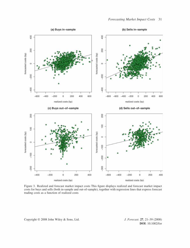
Figure 3 displays scatter diagrams of realized and forecast trading costs, together with regression lines that capture the relation between forecasts and realizations. Clearly, predicted trading costs differ considerably from realized costs. This is confi rmed by formal error measures, such as Theil’s inequality coeffi cient, which takes the value one in the no-skill case and equals zero with perfect foresight. In-sample it takes the value 0.61 for buys and 0.58 for sells. Out-of-sample it equals 0.67 and 0.68, respectively. Several other error measures are displayed in Table III. Similar to Theil’s inequality measure, the mean absolute relative error is a scale-independent measure for the forecast error which should be as close to zero as possible. The mean squared error is another measure for

Table II. Market impact costs and its determinants

Variable Buys Sells

Coeff. t-value Coeff. t-value

intercept −45.6 −1.8 −2.3 −0.1momentumperc 24.5 10.6 -21.4 −9.4tradesizertdv 5.6 2.7 7.7 2.7marketcap 3.6 1.7 -8.9 −3.5agencysingledum 48.6 6.3 −8.5 −0.8quantdum -52.2 −4.5 56.6 4.3preopendum 80.3 6.7 -71.7 −3.9morningdum 81.1 6.6 -86.9 −4.9Wednesdaydum -62.1 −9.0 62.9 6.2Thursdaydum -89.2 −8.1 87.6 5.9Fridaydum -117.7 −11.3 111.1 8.6earlymonthdum 16.3 1.4 46.2 3.1Febdum 46.2 5.9 -40.2 −4.2NYSEdum -56.1 −6.6 66.8 6.6Nasdaqdum -101.4 −7.7 140.0 10.4Adj. R2 0.17 0.23

This table displays a list of determinants of market impact costs and their estimated coeffi cients (together with White’s (1980) heteroskedasticity-robust t-values) based on the model of equation (2) for buys. The same model was estimated for sells. Coeffi cients in bold face are signifi cant at the 5% level.



Figure 3. Realized and forecast market impact costs This fi gure displays realized and forecast market impact costs for buys and sells (both in-sample and out-of-sample), together with regression lines that express forecast trading costs as a function of realized costs



the prediction error, but it depends on the scale of the data. Therefore, we also report its decompo-sition into bias, variance, and covariance percentages which sum up to 100%. The bias percentage tells how far the mean of the forecast is from the mean of the actual series, whereas the variance percentage measures the variation of the forecast relative to the variation of the actual costs. The covariance percentage measures the remaining unsystematic forecasting errors. Ideally, the bias and variance proportions should be small, so that most of the discrepancy between forecast and realized market impact costs is idiosyncratic. The hit ratio counts the percentage of forecasts with the correct sign. Table III also displays the ‘naive’ hit ratio (obtained by assigning each trade to the most likely category). Finally, Table III reports the correlation between the forecast and realized trading costs, which should ideally be as close to one as possible. For more information on the error measures and their defi nitions, we refer to the Appendix.

As expected, the performance of the forecasts is generally better in-sample than out-of-sample. Table III shows that both the in-sample and out-of-sample forecasts have a small bias proportion, but a considerable variance percentage. However, the variance proportion is still much smaller than the covariance percentage. Hence, the forecasts succeed well in capturing the mean of the actual market impact costs, but are less successful in capturing the variation of these costs. Only for sells in the out-of-sample period is the hit ratio of the quantile model lower than the naive hit ratio. The correlations between forecast and realized trading costs refl ect to what extent the model indeed forecasts higher trading costs for stocks that actually incur high costs. Both in-sample and out-of-sample, the correlation is signifi cantly positive, refl ecting a modest positive relation between forecast and realized trading costs.

Since market impact costs refl ect the price movements of a stock during trade execution, the dif-fi culty of forecasting these costs does not come as a complete surprise. Moreover, the out-of-sample month differs substantially from the in-sample period, which also complicates forecasting. That is, January 2002 was bearish and February was quite fl at, but the out-of-sample month of March was bullish. Nevertheless, even for the turbulent out-of-sample month the upward slopes of the regres-sion lines in Figure 3 refl ect fairly positive correlations between realized and forecast trading costs. In-sample the correlations equal 0.44 for buys and 0.50 for sells. Out-of-sample they take values 0.19 and 0.27, respectively. All correlations are signifi cant at a 5% signifi cance level.

Table III. Quality measures for in-sample and out-of-sample forecasts

Buys Sells

In-sample Out-of-sample In-sample Out-of-sample

Theil’s U 0.61 0.67 0.57 0.68Mean absolute percentage error 4.1 8.6 3.2 3.5Mean squared error 12,876 9,283 17,398 11,425Bias part (%) 0.0 0.0 0.0 2.5Variance part (%) 39.0 21.6 33.1 31.8Covariance part (%) 61.1 78.6 66.9 66.0Naive hit ratio (%) 59.2 52.7 50.5 59.1Hit ratio (%) 67.4 57.8 66.3 51.6Correlation to realized costs 0.44 0.19 0.50 0.27

This table displays various quality measures for the in-sample and out-of-sample forecasts of market impact costs based on the standard forecast method derived from the regression model.



Bucket classifi cation approachAlthough the forecast quality of the specifi cation in equation (2) is limited, the model at least suc-ceeds in forecasting higher trading costs for stocks that actually experienced higher costs of trading.7 Therefore, we expect to be more successful in classifying market impact costs in terms of ‘high’ or ‘low’, rather than forecasting exact numeric values.

To predict trading costs in terms of ‘high’ or ‘low’, we distinguish fi ve buckets with predefi ned boundaries. We use the probability to exceed a certain level of market impact costs on a trade (i.e., P(CB > T | X1, . . . , XN)) to predict the bucket in which market impact costs will fall. The higher the probability that a trade will cause high trading costs, the higher the bucket we will predict for that trade. We take the same buckets for buys and sells and defi ne them in such a way that we have fi ve buckets with increasing levels of market impact costs: bucket 1 (‘no costs’, (−∞, 0] bp), bucket 2 (‘low costs’, (0, 20] bp), bucket 3 (‘average costs’, (20, 50] bp), bucket 4 (‘high costs’, (50, 80] bp), bucket 5 (‘severe costs’, (80, ∞) bp). Given p0 = 0 and p5 = 1, we set four critical ‘cut-off prob-abilities’ p1, p2, p3, and p4 to assign the trades to one of the fi ve buckets. If the ‘excess probability’ satisfi es pi < IP(CB > T | X1, . . . , XN) < pi + 1 for a certain critical level T, we predict8 that a buy will fall in bucket i + 1.

We can easily calculate the excess probability corresponding to the regression model in equation (2), provided that we know the distribution of the error term. If we denote the distribution function of the noise term by FB(x) = P(eB ≤ x), the excess probability for buys according to model (2) can be written as

P CB B B B>( ) = − − −

=

∑T F TN j jj

N

X X X1 01

1, ...., β β (3)

The distribution of the noise term has to be known in advance to calculate this probability. As usual, the assumption of normality seems obvious and convenient, but is nevertheless likely to be restrictive. Therefore, we take the empirical distribution of the noise term based on the in-sample period, which avoids any parametric assumptions. This means that we calculate the excess prob-ability as the fraction of trades in the in-sample period for which the residuals9 exceed the value in the parentheses of FB(·) in the excess probability.

In practice, the choice of the critical level and cut-off probabilities will depend on the investor’s preference regarding the balance between the false alarm and the missed detection rate. Here we use the in-sample period to determine appropriate values of the critical level T and the cut-off prob-abilities p1, . . . , p4. We set T = 80 and p1 = 0.10, p2 = 0.175, p3 = 0.275, and p4 = 0.50. For sells we proceed in a similar way and set T = 80 and p1 = 0.09, p2 = 0.15, p3 = 0.25, and p4 = 0.40.

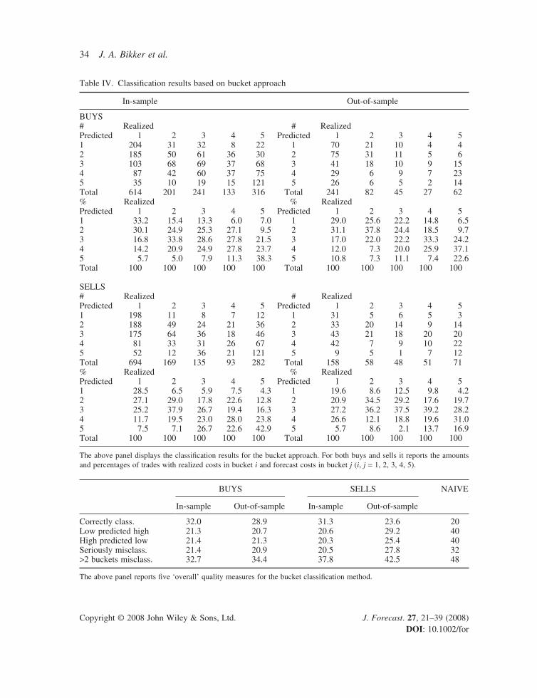
Again we use an expanding estimator and evaluate the quality of the bucket forecasting approach. The upper panel of Table IV displays the classifi cation results, both in absolute numbers and per-centages. Ideally, the percentages on the diagonals of the second and fourth panel at the right-hand side of Table IV should be as close as possible to 100%. The higher they are, the more trades are classifi ed in the correct buckets. Misclassifi cation occurs when off-diagonal elements in Table IV

7 We notice that a correlation between realized and forecast trading costs of x% corresponds to an investor skill of approxi-mately x% as well. 8 Alternatively, we could use linear discriminant analysis or an ordered probit/logit model for this classifi cation problem. However, we obtain better results with the current method. 9 The residuals are defi ned as eB = CB − bB

0 − ΣNj=1bB

j Xj.



Table IV. Classifi cation results based on bucket approach

In-sample Out-of-sample

BUYS# Realized # RealizedPredicted 1 2 3 4 5 Predicted 1 2 3 4 51 204 31 32 8 22 1 70 21 10 4 42 185 50 61 36 30 2 75 31 11 5 63 103 68 69 37 68 3 41 18 10 9 154 87 42 60 37 75 4 29 6 9 7 235 35 10 19 15 121 5 26 6 5 2 14Total 614 201 241 133 316 Total 241 82 45 27 62% Realized % RealizedPredicted 1 2 3 4 5 Predicted 1 2 3 4 51 33.2 15.4 13.3 6.0 7.0 1 29.0 25.6 22.2 14.8 6.52 30.1 24.9 25.3 27.1 9.5 2 31.1 37.8 24.4 18.5 9.73 16.8 33.8 28.6 27.8 21.5 3 17.0 22.0 22.2 33.3 24.24 14.2 20.9 24.9 27.8 23.7 4 12.0 7.3 20.0 25.9 37.15 5.7 5.0 7.9 11.3 38.3 5 10.8 7.3 11.1 7.4 22.6Total 100 100 100 100 100 Total 100 100 100 100 100

SELLS# Realized # RealizedPredicted 1 2 3 4 5 Predicted 1 2 3 4 51 198 11 8 7 12 1 31 5 6 5 32 188 49 24 21 36 2 33 20 14 9 143 175 64 36 18 46 3 43 21 18 20 204 81 33 31 26 67 4 42 7 9 10 225 52 12 36 21 121 5 9 5 1 7 12Total 694 169 135 93 282 Total 158 58 48 51 71% Realized % RealizedPredicted 1 2 3 4 5 Predicted 1 2 3 4 51 28.5 6.5 5.9 7.5 4.3 1 19.6 8.6 12.5 9.8 4.22 27.1 29.0 17.8 22.6 12.8 2 20.9 34.5 29.2 17.6 19.73 25.2 37.9 26.7 19.4 16.3 3 27.2 36.2 37.5 39.2 28.24 11.7 19.5 23.0 28.0 23.8 4 26.6 12.1 18.8 19.6 31.05 7.5 7.1 26.7 22.6 42.9 5 5.7 8.6 2.1 13.7 16.9Total 100 100 100 100 100 Total 100 100 100 100 100

The above panel displays the classifi cation results for the bucket approach. For both buys and sells it reports the amounts and percentages of trades with realized costs in bucket i and forecast costs in bucket j (i, j = 1, 2, 3, 4, 5).

BUYS SELLS NAIVE

In-sample Out-of-sample In-sample Out-of-sample

Correctly class. 32.0 28.9 31.3 23.6 20Low predicted high 21.3 20.7 20.6 29.2 40High predicted low 21.4 21.3 20.3 25.4 40Seriously misclass. 21.4 20.9 20.5 27.8 32>2 buckets misclass. 32.7 34.4 37.8 42.5 48

The above panel reports fi ve ‘overall’ quality measures for the bucket classifi cation method.



are not equal to zero. The lower panel of Table IV displays several measures related to the overall classifi cation quality. We consider the percentage of (1) correctly classifi ed trades, (2) trades with no or low market impact costs that are predicted to have high or severe trading costs, (3) trades with high or severe market impact costs that are predicted to have no or low trading costs, (4) seriously misclassifi ed trades, which are defi ned as trades with no or low costs classifi ed as high or severe or vice versa, and (5) trades misclassifi ed two or more buckets away from the correct bucket. We compare the resulting percentages to the ‘no-skill’ or ‘naive’ model assigning a trade to bucket i = 1, . . . , 5 with probability 1/5. For both buys and sells, the bucket approach strongly outperforms the no-skill method on all fi ve criteria. In particular, the important category of trades with high or severe trading costs that are wrongly classifi ed as having no or low costs is only around 20–25%, versus 40% in the no-skill model. In line with expectations, the performance of the bucket approach relative to the naive model is in-sample more convincing than out-of-sample. However, the out-of-sample performance is still very good.

Identifying expensive trades: probability methodAnother way of dealing with future market impact costs is to identify trades that have a high chance of being (too) expensive. That is, we assume that a trade is identifi ed as expensive when the excess probability exceeds a certain critical level; i.e., when P(CB > T | X1, . . . , XN) ≥ p, for certain investor-specifi c values of the critical level T and cut-off probability p. The difference between this ‘probability method’ and the previous two approaches is that we no longer forecast a level or range of market impact costs for each trade, but only identify those that are likely to be expensive. Again we use the empirical distribution to calculate the excess probability.

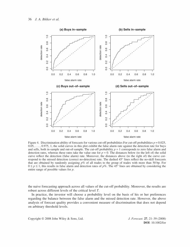
To assess how well the probability method discriminates between cheap and expensive trades, we set the critical level at T = 50. For cut-off probabilities p = 0.025, 0.05, . . . , 0.975, 1, we plot the cor-responding false alarm rates against the detection rates. The solid curves in Figure 4 highlight several relevant quantities for buys and sells, both in-sample and out-of-sample. The distances below (to the left of) the solid curves refl ect the detection (false alarm) rate. Moreover, the distances above (to the right of) the curves correspond to the missed detection (correct no-detection) rate. For instance, p = 0.25 results in false alarm and detection rates of, respectively, 54% and 83% (in-sample) and 47% and 82% (out-of-sample) for buys. For sells these rates equal 43% and 75% (in-sample) and 46% and 64% (out-of-sample). In the case of perfect foresight, the detection rate equals 100% at each false alarm rate. The dashed 45° lines in Figure 4 refl ect the no-skill forecasts that are obtained by randomly assigning p% of all trades to the group of trades with costs higher than 50 bp. For 0 ≤ p ≤ 1, this results in false alarm and detection rates of p%. The 45° lines are obtained by considering the entire range of possible values for the cut-off probability p. From Figure 4 we see that at each level of the false alarm rate the probability method has a higher detection rate than the no-skill method.

The surface of the areas below each solid curve can be viewed as the proportion of correct forecasts across all possible thresholds. This surface ranges from 0 to 100%, where the value 50% corresponds to the no-skill value (which equals the surface of the area under the 45° line) and 100% to perfect foresight. It serves as a summary statistic of the discrimination power of the model. For buys, its value equals 76% for the in-sample period and 77% for the out-of-sample period. For sells, it takes the values 78% and 68%, respectively.10 Hence the probability method substantially outperforms

10 We have calculated the surfaces using the trapezoidal rule for numerical integration based on 40 points.



the naive forecasting approach across all values of the cut-off probability. Moreover, the results are robust across different levels of the critical level T.

In practice, the investor will choose a probability level on the basis of his or her preferences regarding the balance between the false alarm and the missed detection rate. However, the above analysis of forecast quality provides a convenient measure of discrimination that does not depend on arbitrary threshold levels.

0.0 0.2 0.4 0.6 0.8 1.0

0.0

0.2

0.4

0.6

0.8

1.0

false alarm rate

dete

ctio

n ra

te

(a) Buys in−sample

0.0 0.2 0.4 0.6 0.8 1.0

0.0

0.2

0.4

0.6

0.8

1.0

false alarm rate

dete

ctio

n ra

te

(b) Sells in−sample

0.0 0.2 0.4 0.6 0.8 1.0

0.0

0.2

0.4

0.6

0.8

1.0

false alarm rate

dete

ctio

n ra

te

(c) Buys out−of−sample

0.0 0.2 0.4 0.6 0.8 1.0

0.0

0.2

0.4

0.6

0.8

1.0

false alarm rate

dete

ctio

n ra

te

(d) Sells out−of−sample

Figure 4. Discrimination ability of forecasts for various cut-off probabilities For cut-off probabilities p = 0.025, 0.05, . . . , 0.975, 1, the solid curves in this plot exhibit the false alarm rate against the detection rate for buys and sells, both in-sample and out-of-sample. The cut-off probability p = 1 corresponds to zero false alarm and detection rates, whereas these rates take the value one for p = 0. The distances below (to the left of) the solid curve refl ect the detection (false alarm) rate. Moreover, the distances above (to the right of) the curve cor-respond to the missed detection (correct no-detection) rate. The dashed 45° lines refl ect the no-skill forecasts that are obtained by randomly assigning p% of all trades to the group of trades with more than 50 bp. For 0 ≤ p ≤ 1, this results in false alarm and detection rates of p%. The 45° lines are obtained by considering the entire range of possible values for p.



INTEGRATING MARKET IMPACT COSTS IN THE EQUITY INVESTMENT PROCESS

Portfolio management is an economic decision problem dealing with the trade-off between expected returns, risk, and transaction costs. In this section we discuss how our forecasting model for trading costs as given in equation (2) can be employed for making better-informed decisions in portfolio management. We do not strive to discuss the above economic decision problem in detail here, as an excellent treatment can be found in Grinold and Kahn (1999). Here we limit ourselves to the concepts and focus on our contribution to a better specifi cation of the cost function.

As advocated by Grinold and Kahn (1999), we opt for a full integration of forecasts of transaction costs, particularly market impact costs, in portfolio construction at the same stage of the optimiza-tion process where risk and return forecasts are used. In this way the components return, risk, and costs are optimized simultaneously. We note that the above costs not only refer to transaction costs but also to either self-imposed constraints or constraints that are imposed by the regulator. This integrated approach is especially relevant in case restrictions are added to the portfolio allocation problem. In such cases a sequential approach, rather than an integrated approach, could lead to less optimal portfolio allocations. For example, a long–short equity manager may carefully construct a market neutral portfolio by imposing zero exposures to certain style factors. If subsequently certain stocks are allocated different weights on the basis of the transaction cost analysis, the fi nal portfolio may be far from market-neutral.

In short, the trade-off between return, risk, and costs can be formalized by expressing the follow-ing investor utility function:11

U w w w c w= ′ − ( ) ′ − ( )µ λ κ2 Σ (4)

Here w are the portfolio weights, m are the expected returns, Σ is the covariance matrix of the returns and c(·) is the cost function. Furthermore, l > 0 and k > 0 are, respectively, the risk aversion and the cost aversion parameter.

The risk–return trade-off problem has been well understood since the landmark analysis by Markowitz (1952) on mean–variance effi ciency and Sharpe’s (1964) CAPM model. The incor-poration of costs in the development of optimal strategies complicates the analysis and is still an underdeveloped area in fi nancial economics. We refer to Grinold (2006) for a recent attempt of integrating costs in the theory of portfolio management. The costs function c(·) is usually specifi ed as a function of w only. For example, Keim and Madhaven (1996) fi nd that market impact costs increase with three-halves power of the size of the trade, i.e., c(w) ∝ w3/2. Grinold (2006) works with c(w) ∝ w2. The contribution of our paper is that we come up with a broader specifi cation of c(·). That is, our function c(·) is not only a function of the weights w but also of the risk factors X1, . . . , XN in our model in equation (2). We note that some of these variables, such as volatility and momentum, are exogenous to the decision maker. Other determinants, such as the day of the week and the agency–principal dummy, are under the control of the decision maker, so these in turn can be integrated in the utility framework in equation (4) above.

Estimation errors may dominate portfolio construction in practice, particularly when the uncer-tainty about the market impact cost estimate is much larger than the mean. More accurate specifi ca-tion of the cost function c(·) in equation (4) will improve portfolio optimization. Additionally, the

11 We follow the usual mean–variance framework in our specifi cation of the expected utility function.



market impact cost model can be used to identify which factors (e.g., percentage of average daily volume) attribute most to market impact. Such insights can be used to control the active bets in a similar way that other investment constraints do.

The cost forecasts can also be used to identify potentially expensive trades in terms of market impact costs. Such forecasts have a signaling function in the trade-monitoring phase. A different trading strategy can be adopted for trades that are likely to turn out expensive.

CONCLUSIONS

When a relatively small group of trades causes the major part of the market impact costs of an investment portfolio, a reduction of the trading costs of comparatively few expensive trades would already result in substantial savings on total trading costs. For the global equity trades analyzed in this paper, executed by the world’s second largest pension fund ABP in the fi rst quarter of 2002, we fi nd that only 10% of the trades causes 75% of total trading costs. Simulations emphasize that there is a strong nonlinear trade-off between trading costs and the number of trades executed.

Since trading costs depend to some extent on controllable factors such as broker intermediation, trade timing, and trading venue, investors may reduce the costs of trading by carefully controlling these factors. As a fi rst step in this direction, this paper has proposed two methods to identify poten-tially expensive trades. The bucket classifi cation method predicts the category trading costs will fall into. The probability approach detects expensive trades on the basis of the probability that market impact costs will exceed a particular level. Applied to the equity trades executed by ABP, the pro-posed methods succeed in identifying a considerable number of expensive trades and substantially outperform no-skill prediction methods. However, we emphasize that the forecasting power of any model at a certain moment in time does not necessarily carry over to the future. Continuous updating of forecasting models, both in terms of functional form and model coeffi cients, will be necessary to adapt to changes in the market environment.

The results of this paper illustrate the productive role that model-based forecasts can play in trading cost management. This role can be extended further when the cost forecasts are integrated with the risk–return optimization process of portfolio allocations.

ACKNOWLEDGEMENTS

The authors would like to thank the participants of the research seminars at De Nederlandsche Bank, University of Twente, and Delft University of Technology. We are also grateful to the participants of the 9th Conference of the Swiss Society for Financial Market Research in Zürich and the Math-ematical PhD Day in Utrecht. In particular, we would like thank Alain Durré for his useful feedback. The usual disclaimer applies. The views expressed in this paper are not necessarily shared by DNB and ABP or its subsidiaries.

REFERENCES

Almgren R, Thum C, Hauptmann E, Li H. 2005. Equity market impact. Latin Risk September: 21–28.Bikker JA, Spierdijk L, Van der Sluis PJ. 2007. Market impact costs of institutional equity trades. Journal of

International Money and Finance 26: 974–1000.



Chan LKC, Lakonishok J. 1995. The behavior of stock prices around institutional trades. Journal of Finance 50: 1147–1174.

Chan LKC, Lakonishok J. 1997. Institutional equity trading costs: NYSE versus Nasdaq. Journal of Finance 52: 713–735.

Cheng M. 2003. Pretrade cost analysis and management of implementation shortfall. AIMR Conference Proceedings July: 26–34.

Grinold RC. 2006. Implementation effi ciency. Investment Insights 4.06. Barclays Global Investors: San Francisco, CA.

Grinold RC, Kahn RN. 1999. Active Portfolio Management: A Quantitative Approach for Producing Superior Returns and Selecting Superior Returns and Controlling Risk. McGraw-Hill: New York.

Keim DB, Madhavan A. 1996. The upstairs market for large-block transactions: analysis and measurement of price effects. Review of Financial Studies 9: 1–36.

Keim DB, Madhavan A. 1998. The cost of institutional equity trades. Financial Analysts Journal 54: 50–69.Konstance MS. 2003. Trading cost analysis and management. AIMR Conference Proceedings July: 8–12.Markowitz HM. 1952. Portfolio selection. Journal of Finance 7: 77–91.Sharpe WF. 1964. Capital asset prices: a theory of market equilibrium under conditions of risk. Journal of Finance

19: 425–442.Wagner WH, Edwards M. 1993. Best execution. Financial Analysts Journal 49: 65–71.White H. 1980. Heteroskedasticity consistent covariance matrix estimator and a direct test for heteroskedasticity,

Econometrica 48: 817–838.

APPENDIX: FORECAST ERROR MEASURES

Given a sample of observations C1, . . . , Cn and corresponding forecasts C1, . . . , CN the mean abso-lute percentage error (MAPE) is defi ned as

MAPE = −=∑1

1n

C C

Ci i

ii

n ˆ (A.1)

Furthermore, the mean squared error (MSE) is calculated as

MSE = −( )=∑1 2

1nC Ci i

i

nˆ (A.2)

The bias, variance, and covariance proportions of the MSE are given by

BP VP CP=−( )−( )

=−( )

−( )=

= =∑ ∑

ˆ

ˆ,

ˆ,

ˆC C

C C n

s s

C C ni ii

n

C C

i ii

n2

1

2

2

1

2 1−−( )−( )=∑ˆ

ˆˆρ s s

C C n

C C

i ii

n 2

1

where C–,

–C, sC, sC are the sample means and variances of C1, . . . , Cn and C1, . . . , Cn, respectively.

The sample correlation between the series of observed values and forecasts is denoted by r. Finally, Theil’s inequality coeffi cient is obtained as

UC C

C C

n i

n

i i

n i

ni n i

ni

=−( )

+

=

= =

∑

∑ ∑

11

2

1

12 1

12

ˆ

ˆ (A.3)

forecasting market impact costs and identifying expensive trades

Documents