Forecasting Human Dynamics from Static Images

Yu-Wei Chao1, Jimei Yang2, Brian Price2, Scott Cohen2, and Jia Deng1

1University of Michigan, Ann Arbor

{ywchao,jiadeng}@umich.edu

2Adobe Research

{jimyang,bprice,scohen}@adobe.com

Abstract

This paper presents the first study on forecasting human

dynamics from static images. The problem is to input a sin-

gle RGB image and generate a sequence of upcoming hu-

man body poses in 3D. To address the problem, we propose

the 3D Pose Forecasting Network (3D-PFNet). Our 3D-

PFNet integrates recent advances on single-image human

pose estimation and sequence prediction, and converts the

2D predictions into 3D space. We train our 3D-PFNet using

a three-step training strategy to leverage a diverse source

of training data, including image and video based human

pose datasets and 3D motion capture (MoCap) data. We

demonstrate competitive performance of our 3D-PFNet on

2D pose forecasting and 3D pose recovery through quanti-

tative and qualitative results.

1. Introduction

Human pose forecasting is the capability of predicting

future human body dynamics from visual observations. Hu-

man beings are endowed with this great ability. For exam-

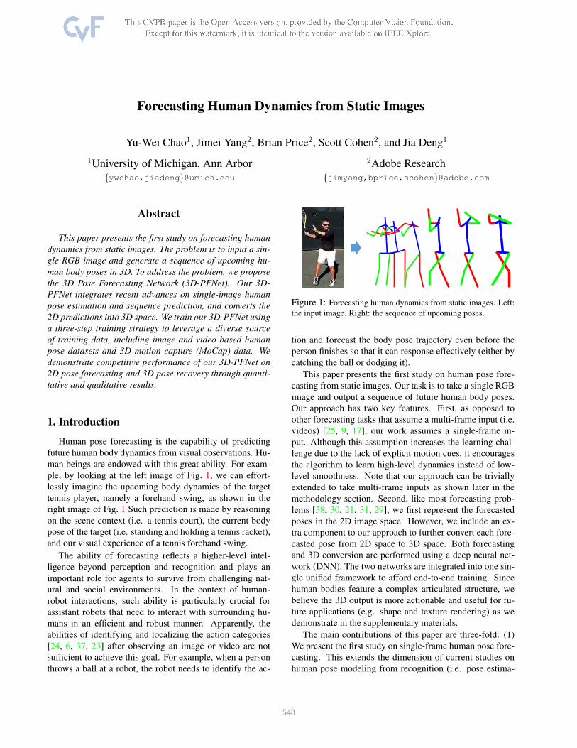
ple, by looking at the left image of Fig. 1, we can effort-

lessly imagine the upcoming body dynamics of the target

tennis player, namely a forehand swing, as shown in the

right image of Fig. 1 Such prediction is made by reasoning

on the scene context (i.e. a tennis court), the current body

pose of the target (i.e. standing and holding a tennis racket),

and our visual experience of a tennis forehand swing.

The ability of forecasting reflects a higher-level intel-

ligence beyond perception and recognition and plays an

important role for agents to survive from challenging nat-

ural and social environments. In the context of human-

robot interactions, such ability is particularly crucial for

assistant robots that need to interact with surrounding hu-

mans in an efficient and robust manner. Apparently, the

abilities of identifying and localizing the action categories

[24, 6, 37, 23] after observing an image or video are not

sufficient to achieve this goal. For example, when a person

throws a ball at a robot, the robot needs to identify the ac-

Figure 1: Forecasting human dynamics from static images. Left:

the input image. Right: the sequence of upcoming poses.

tion and forecast the body pose trajectory even before the

person finishes so that it can response effectively (either by

catching the ball or dodging it).

This paper presents the first study on human pose fore-

casting from static images. Our task is to take a single RGB

image and output a sequence of future human body poses.

Our approach has two key features. First, as opposed to

other forecasting tasks that assume a multi-frame input (i.e.

videos) [25, 9, 17], our work assumes a single-frame in-

put. Although this assumption increases the learning chal-

lenge due to the lack of explicit motion cues, it encourages

the algorithm to learn high-level dynamics instead of low-

level smoothness. Note that our approach can be trivially

extended to take multi-frame inputs as shown later in the

methodology section. Second, like most forecasting prob-

lems [38, 30, 21, 31, 29], we first represent the forecasted

poses in the 2D image space. However, we include an ex-

tra component to our approach to further convert each fore-

casted pose from 2D space to 3D space. Both forecasting

and 3D conversion are performed using a deep neural net-

work (DNN). The two networks are integrated into one sin-

gle unified framework to afford end-to-end training. Since

human bodies feature a complex articulated structure, we

believe the 3D output is more actionable and useful for fu-

ture applications (e.g. shape and texture rendering) as we

demonstrate in the supplementary materials.

The main contributions of this paper are three-fold: (1)

We present the first study on single-frame human pose fore-

casting. This extends the dimension of current studies on

human pose modeling from recognition (i.e. pose estima-

548

tion [27, 19]) to forecasting. The problem of pose fore-

casting in fact generalizes pose estimation, since to fore-

cast future poses we need to first estimate the observed

pose. (2) We propose a novel DNN-based approach to ad-

dress the problem. Our forecasting network integrates re-

cent advances on single-image human pose estimation and

sequence prediction. Experimental results show that our ap-

proach outperforms strong baselines on 2D pose forecast-

ing. (3) We propose an extra network to convert the fore-

casted 2D poses into 3D skeletons. Our 3D recovery net-

work is trained on a vast amount of synthetic examples by

leveraging motion capture (MoCap) data. Experimental re-

sults show that our approach outperforms two state-of-the-

art methods on 3D pose recovery. In a nutshell, we propose

a unified framework for 2D pose forecasting and 3D pose

recovery. Our 3D Pose Forecasting Network (3D-PFNet)

is trained by leveraging a diverse source of training data,

including image and video based human pose datasets and

MoCap data. We separately evaluate our 3D-PFNet on 2D

pose forecasting and 3D pose recovery, and show competi-

tive results over baselines.

2. Related Work

Visual Scene Forecasting Our work is in line with a se-

ries of recent work on single-image visual scene forecast-

ing. These works vary in the predicted target and the output

representation. [15] predicts human actions in the form of

semantic labels. Some others predict motions of low level

image features, such as the optical flow to the next frame

[21, 31] or dense trajectories of pixels [38, 29]. A few oth-

ers attempt to predict the motion trajectories of middle-level

image patches [30] or rigid objects [18]. However, these

methods do not explicitly output a human body model, thus

cannot directly address human pose forecasting. Notably,

[9] predicts the future dynamics of a 3D human skeleton

from its past motion. Despite its significance, their method

can be applied to only 3D skeleton data but not visual in-

puts. Our work is the first attempt to predict 3D human

dynamics from RGB images.

Human Pose Estimation Our work is closely related to

the problem of human pose estimation, which has long been

attractive in computer vision. Human bodies are commonly

represented by tree-structured skeleton models, where each

node is a body joint and the edges capture articulation. The

goal is to estimate the 2D joint locations in the observed im-

age [27, 19] or video sequences [20, 10]. Recent work has

even taken one step further to directly recover 3D joint lo-

cations [16, 36, 26, 7, 4, 22] or body shapes [3] from image

observations. While promising, these approaches can only

estimate the pose of humans in the observed image or video.

Our approach not only estimate the human pose in the ob-

served image, but also forecasts the poses in the upcoming

Input Image

Pose Sequence

�� �� ��+1 ��+

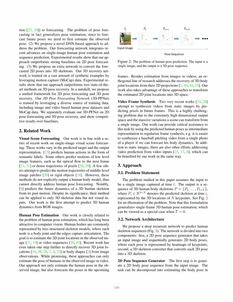
Figure 2: The problem of human pose prediction. The input is a

single image, and the output is a 3D pose sequence.

frames. Besides estimation from images or videos, an or-

thogonal line of research addresses the recovery of 3D body

joint locations from their 2D projections [1, 40, 41, 32]. Our

work also takes advantage of these approaches to transform

the estimated 2D joint locations into 3D space.

Video Frame Synthesis Two very recent works [33, 28]

attempt to synthesize videos from static images by pre-

dicting pixels in future frames. This is a highly challeng-

ing problem due to the extremely high dimensional output

space and the massive variations a scene can transform from

a single image. Our work can provide critical assistance to

this task by using the predicted human poses as intermediate

representation to regularize frame synthesis, e.g. it is easier

to synthesize a baseball pitching video from a single photo

of a player if we can forecast his body dynamics. In addi-

tion to static images, there are also other efforts addressing

video prediction from video inputs [25, 17, 8], which can

be benefited by our work in the same way.

3. Approach

3.1. Problem Statement

The problem studied in this paper assumes the input to

be a single image captured at time t. The output is a se-

quence of 3D human body skeletons P = {Pt, . . . , Pt+T },

where Pi ∈ R3×N denotes the predicted skeleton at time i,

represented by the 3D locations of N keypoints. See Fig. 2

for an illustration of the problem. Note that this formulation

generalizes single-frame 3D human pose estimation, which

can be viewed as a special case when T = 0.

3.2. Network Architecture

We propose a deep recurrent network to predict human

skeleton sequences (Fig. 3). The network is divided into two

components: first, a 2D pose sequence generator that takes

an input image and sequentially generates 2D body poses,

where each pose is represented by heatmaps of keypoints;

second, a 3D skeleton converter that converts each 2D pose

into a 3D skeleton.

2D Pose Sequence Generator The first step is to gener-

ate a 2D body pose sequence from the input image. The

task can be decomposed into estimating the body pose in

549

RNN

Encoder

Decoder

3D Skeleton

Converter

2D Pose

Sequence

Generator

Input Image

2D Pose

Heatmaps

3D Skeleton

Hourglass network [18]

Encoder Decoder

0 0

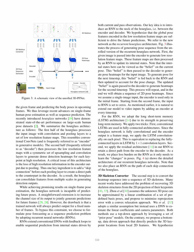
Figure 3: A schematic view of the unrolled 3D-PFNet.

the given frame and predicting the body poses in upcoming

frames. We thus leverage recent advances on single-frame

human pose estimation as well as sequence prediction. The

recently introduced hourglass networks [19] have demon-

strated state-of-the-art performance on large-scale human

pose datasets [2]. We summarize the hourglass architec-

ture as follows: The first half of the hourglass processes

the input image with convolution and pooling layers to a

set of low resolution feature maps. This resembles conven-

tional ConvNets (and is frequently referred to as “encoder”

in generative models). The second half (frequently referred

to as “decoder”) then processes the low resolution feature

maps with a symmetric set of upsampling and convolution

layers to generate dense detection heatmaps for each key-

point at high resolution. A critical issue of this architecture

is the loss of high resolution information in the encoder out-

put due to pooling. Thus one key ingredient is to add a “skip

connection” before each pooling layer to create a direct path

to the counterpart in the decoder. As a result, the hourglass

can consolidate features from multiple scales in generating

detection outputs.

While achieving promising results on single-frame pose

estimation, the hourglass network is incapable of predict-

ing future poses. A straightforward extension is to increase

the channel size of its output to jointly generate predictions

for future frames [29, 28]. However, the drawback is that a

trained network will always predict output for a fixed num-

ber of frames. To bypass this constraint, we choose to for-

mulate pose forecasting as a sequence prediction problem

by adopting recurrent neural networks (RNNs).

RNNs extend conventional DNNs with feedback loops to

enable sequential prediction from internal states driven by

both current and pass observations. Our key idea is to intro-

duce an RNN to the neck of the hourglass, i.e. between the

encoder and decoder. We hypothesize that the global pose

features encoded in the low resolution feature maps are suf-

ficient to drive the future predictions. We refer to the new

network as the recurrent hourglass architecture. Fig. 3 illus-

trates the process of generating pose sequence from the un-

rolled version of the recurrent hourglass network. First, the

given image is passed into the encoder to generate low reso-

lution feature maps. These feature maps are then processed

by an RNN to update its internal states. Note that the inter-

nal states here can be viewed as the “belief” on the current

pose. This “belief” is then passed to the decoder to gener-

ate pose heatmaps for the input image. To generate pose for

the next timestep, this “belief” is fed back to the RNN and

then updated to account for the pose change. The updated

“belief” is again passed to the decoder to generate heatmaps

for the second timestep. This process will repeat, and in the

end we will obtain a sequence of 2D pose heatmaps. Since

we assume a single-image input, the encoder is used only in

the initial frame. Starting from the second frame, the input

to RNN is set to zeros. As mentioned earlier, it is natural to

extend our model to video inputs by adding an encoder at

every timestep.

For the RNN, we adopt the long short-term memory

(LSTM) architecture [14] due to its strength in preserving

long-term memory. We apply two tricks: First, conventional

LSTMs are used in fully-connected architectures. Since the

hourglass network is fully convolutional and the encoder

output is a feature map, we apply the LSTM convolution-

ally on each pixel. This is equivalent to replacing the fully-

connected layers in LSTM by 1×1 convolution layers. Sec-

ond, we apply the residual architecture [11] in our RNN to

retain a direct path from the encoder to the decoder. As a

result, we place less burden on the RNN as it only needs to

learn the “changes” in poses. Fig. 4 (a) shows the detailed

architecture of our recurrent hourglass networks. Note that

we also place an RNN on the path of each skip connection

of the hourglass.

3D Skeleton Converter The second step is to convert the

heatmap sequence into a sequence of 3D skeletons. Many

recent works have addressed the problem of recovering 3D

skeleton structures from the 2D projection of their keypoints

[40, 32]. Zhou et al.[40] assumes the unknown 3D pose can

be approximated by a linear combination of a set of pre-

defined basis poses, and propose to minimize reprojection

error with a convex relaxation approach. Wu et al. [32]

adopts a similar assumption but instead uses a DNN to es-

timate the linear coefficients and camera parameters. Both

methods use a top-down approach by leveraging a set of

“prior pose” models. On the contrary, we propose a bottom-

up, data driven approach that directly predicts the 3D key-

point locations from local 2D features. We hypothesize

550

RNN

RNN

RNN

RNN

RNN

Projection

Layer

Encoder Decoder

3D Skeleton

Converter

Input Image2D Pose

Heatmaps

3D Keypoint Location

Relative to Center

3D Translation to

Center

Camera Focal Length

3D Skeleton

(Training Only)

Conv

LSTM

RNN ℎ�−1 ��−1

ℎ� ��

Conv FC

2D Keypoint

Location

�����

Skip

Connections

(a) (b)

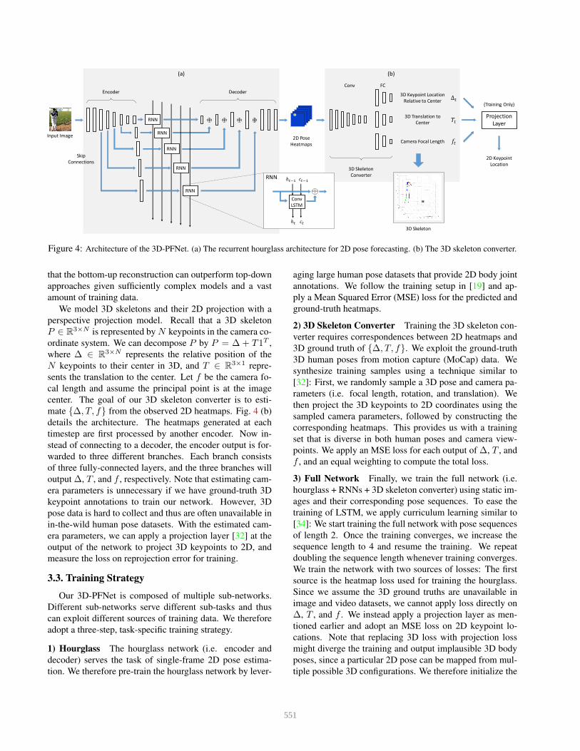
Figure 4: Architecture of the 3D-PFNet. (a) The recurrent hourglass architecture for 2D pose forecasting. (b) The 3D skeleton converter.

that the bottom-up reconstruction can outperform top-down

approaches given sufficiently complex models and a vast

amount of training data.

We model 3D skeletons and their 2D projection with a

perspective projection model. Recall that a 3D skeleton

P ∈ R3×N is represented by N keypoints in the camera co-

ordinate system. We can decompose P by P = ∆ + T1T ,

where ∆ ∈ R3×N represents the relative position of the

N keypoints to their center in 3D, and T ∈ R3×1 repre-

sents the translation to the center. Let f be the camera fo-

cal length and assume the principal point is at the image

center. The goal of our 3D skeleton converter is to esti-

mate {∆, T, f} from the observed 2D heatmaps. Fig. 4 (b)

details the architecture. The heatmaps generated at each

timestep are first processed by another encoder. Now in-

stead of connecting to a decoder, the encoder output is for-

warded to three different branches. Each branch consists

of three fully-connected layers, and the three branches will

output ∆, T , and f , respectively. Note that estimating cam-

era parameters is unnecessary if we have ground-truth 3D

keypoint annotations to train our network. However, 3D

pose data is hard to collect and thus are often unavailable in

in-the-wild human pose datasets. With the estimated cam-

era parameters, we can apply a projection layer [32] at the

output of the network to project 3D keypoints to 2D, and

measure the loss on reprojection error for training.

3.3. Training Strategy

Our 3D-PFNet is composed of multiple sub-networks.

Different sub-networks serve different sub-tasks and thus

can exploit different sources of training data. We therefore

adopt a three-step, task-specific training strategy.

1) Hourglass The hourglass network (i.e. encoder and

decoder) serves the task of single-frame 2D pose estima-

tion. We therefore pre-train the hourglass network by lever-

aging large human pose datasets that provide 2D body joint

annotations. We follow the training setup in [19] and ap-

ply a Mean Squared Error (MSE) loss for the predicted and

ground-truth heatmaps.

2) 3D Skeleton Converter Training the 3D skeleton con-

verter requires correspondences between 2D heatmaps and

3D ground truth of {∆, T, f}. We exploit the ground-truth

3D human poses from motion capture (MoCap) data. We

synthesize training samples using a technique similar to

[32]: First, we randomly sample a 3D pose and camera pa-

rameters (i.e. focal length, rotation, and translation). We

then project the 3D keypoints to 2D coordinates using the

sampled camera parameters, followed by constructing the

corresponding heatmaps. This provides us with a training

set that is diverse in both human poses and camera view-

points. We apply an MSE loss for each output of ∆, T , and

f , and an equal weighting to compute the total loss.

3) Full Network Finally, we train the full network (i.e.

hourglass + RNNs + 3D skeleton converter) using static im-

ages and their corresponding pose sequences. To ease the

training of LSTM, we apply curriculum learning similar to

[34]: We start training the full network with pose sequences

of length 2. Once the training converges, we increase the

sequence length to 4 and resume the training. We repeat

doubling the sequence length whenever training converges.

We train the network with two sources of losses: The first

source is the heatmap loss used for training the hourglass.

Since we assume the 3D ground truths are unavailable in

image and video datasets, we cannot apply loss directly on

∆, T , and f . We instead apply a projection layer as men-

tioned earlier and adopt an MSE loss on 2D keypoint lo-

cations. Note that replacing 3D loss with projection loss

might diverge the training and output implausible 3D body

poses, since a particular 2D pose can be mapped from mul-

tiple possible 3D configurations. We therefore initialize the

551

3D converter network with weights learned from the syn-

thetic data, and keep the weights fixed during the training

of the full network.

4. Experiments

We evaluate our 3D-PFNet on two tasks: (1) 2D pose

forecasting and (2) 3D pose recovery.

4.1. 2D Pose Forecasting

Dataset We evaluate pose forecasting in 2D using the

Penn Action dataset [39]. Penn Action contains 2326 video

sequences (1258 for training and 1068 for test) covering 15

sports action categories. Each video frame is annotated with

a human bounding box along with the locations and visi-

bility of 13 body joints. Note that we do not evaluate our

forecasted 3D poses due to the lack of 3D annotations in

Penn Action. During training, we also leverage two other

datasets: MPII Human Pose (MPII) [2] and Human3.6M

[12]. MPII is a large-scale benchmark for single-frame hu-

man pose estimation. Human3.6M consists of videos of act-

ing individuals captured in a controlled environment. Each

frame is provided with the calibrated camera parameters

and the 3D human pose acquired from MoCap devices.

Evaluation Protocal We preprocess Penn Action with

two steps: First, since our focus is not on human detec-

tion, we crop each video frame to focus roughly around

the human region: for each video sequence, we crop every

frame using the tight box that bounds the human bounding

box across all frames. Second, we do not assume the in-

put image is always the starting frame of each video (i.e.

we should be able to forecast poses not only from the be-

ginning of a tennis forehand swing, but also from the mid-

dle or even shortly before the action finishes). Thus for a

video with K frames, we generate K sequences by varying

the starting frame. Besides, since adjacent frames contain

similar poses, we skip frames when generating sequences.

The number of frames skipped is video-dependent: Given a

sampled starting frame, we always generate a sequence of

length 16, where we skip every (K − 1)/15 frames in the

raw video sequence after the sampled starting frame. This

is to ensure that our forecasted output can “finish” each ac-

tion in a predicted sequence of length 16. Note that once

we surpass the end frame of a video, we will repeat the last

frame collected until we obtain 16 frames. This is to force

the forecasting to learn to “stop” and remain at the ending

pose once an action has completed. Fig. 5 shows sample

sequences of our processed Penn Action.

To evaluate the forecasted pose, we adopt the standard

Percentage of Correct Keypoints (PCK) metric [2] from 2D

pose estimation. PCK measures the accuracy of keypoint

localization by considering a predicted keypoint correct if it

falls within certain normalized distance of the ground truth.

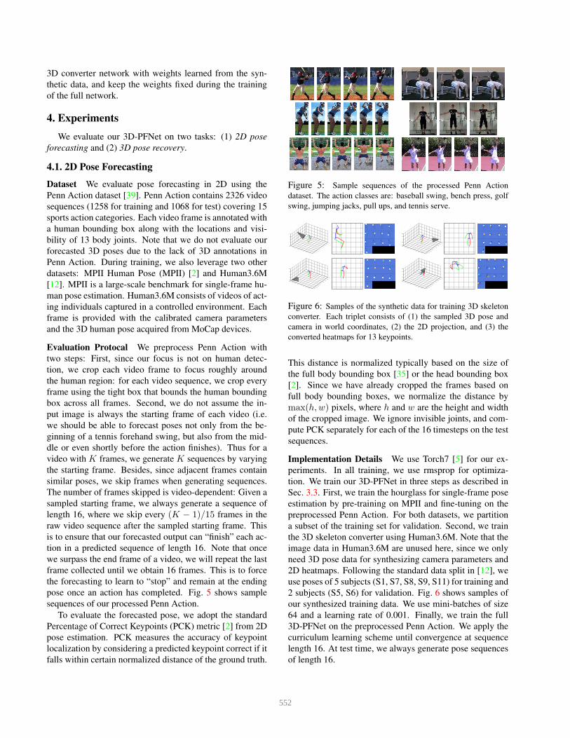
Figure 5: Sample sequences of the processed Penn Action

dataset. The action classes are: baseball swing, bench press, golf

swing, jumping jacks, pull ups, and tennis serve.

−2000

−1500

−1000

−500

0

500

1000

1500

2000−2000

−1500

−1000

−500

0

500

1000

1500

2000

−1000

−500

0

500

1000

−2000

−1500

−1000

−500

0

500

1000

1500

2000−2000

−1500

−1000

−500

0

500

1000

1500

2000

−1000

−500

0

500

1000

−2000

−1500

−1000

−500

0

500

1000

1500

2000−2000

−1500

−1000

−500

0

500

1000

1500

2000

−1000

−500

0

500

1000

−2000

−1500

−1000

−500

0

500

1000

1500

2000−2000

−1500

−1000

−500

0

500

1000

1500

2000

−1000

−500

0

500

1000

Figure 6: Samples of the synthetic data for training 3D skeleton

converter. Each triplet consists of (1) the sampled 3D pose and

camera in world coordinates, (2) the 2D projection, and (3) the

converted heatmaps for 13 keypoints.

This distance is normalized typically based on the size of

the full body bounding box [35] or the head bounding box

[2]. Since we have already cropped the frames based on

full body bounding boxes, we normalize the distance by

max(h,w) pixels, where h and w are the height and width

of the cropped image. We ignore invisible joints, and com-

pute PCK separately for each of the 16 timesteps on the test

sequences.

Implementation Details We use Torch7 [5] for our ex-

periments. In all training, we use rmsprop for optimiza-

tion. We train our 3D-PFNet in three steps as described in

Sec. 3.3. First, we train the hourglass for single-frame pose

estimation by pre-training on MPII and fine-tuning on the

preprocessed Penn Action. For both datasets, we partition

a subset of the training set for validation. Second, we train

the 3D skeleton converter using Human3.6M. Note that the

image data in Human3.6M are unused here, since we only

need 3D pose data for synthesizing camera parameters and

2D heatmaps. Following the standard data split in [12], we

use poses of 5 subjects (S1, S7, S8, S9, S11) for training and

2 subjects (S5, S6) for validation. Fig. 6 shows samples of

our synthesized training data. We use mini-batches of size

64 and a learning rate of 0.001. Finally, we train the full

3D-PFNet on the preprocessed Penn Action. We apply the

curriculum learning scheme until convergence at sequence

length 16. At test time, we always generate pose sequences

of length 16.

552

0 0.02 0.04 0.06 0.08 0.1

0

0.2

0.4

0.6

0.8

1

Hourglass [19]

NN−all

NN−Caffenet

NN−oracle

3D−PPNet

Timestep 1

0 0.02 0.04 0.06 0.08 0.1

0

0.2

0.4

0.6

0.8

1

Timestep 2

0 0.02 0.04 0.06 0.08 0.1

0

0.2

0.4

0.6

0.8

1

Timestep 4

0 0.02 0.04 0.06 0.08 0.1

0

0.2

0.4

0.6

0.8

1

Timestep 8

0 0.02 0.04 0.06 0.08 0.1

0

0.2

0.4

0.6

0.8

1

Timestep 16

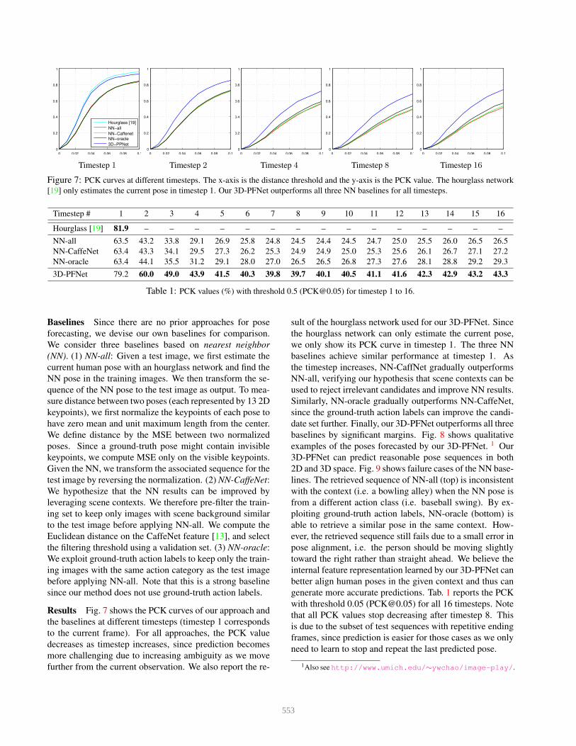
Figure 7: PCK curves at different timesteps. The x-axis is the distance threshold and the y-axis is the PCK value. The hourglass network

[19] only estimates the current pose in timestep 1. Our 3D-PFNet outperforms all three NN baselines for all timesteps.

Timestep # 1 2 3 4 5 6 7 8 9 10 11 12 13 14 15 16

Hourglass [19] 81.9 – – – – – – – – – – – – – – –

NN-all 63.5 43.2 33.8 29.1 26.9 25.8 24.8 24.5 24.4 24.5 24.7 25.0 25.5 26.0 26.5 26.5

NN-CaffeNet 63.4 43.3 34.1 29.5 27.3 26.2 25.3 24.9 24.9 25.0 25.3 25.6 26.1 26.7 27.1 27.2

NN-oracle 63.4 44.1 35.5 31.2 29.1 28.0 27.0 26.5 26.5 26.8 27.3 27.6 28.1 28.8 29.2 29.3

3D-PFNet 79.2 60.0 49.0 43.9 41.5 40.3 39.8 39.7 40.1 40.5 41.1 41.6 42.3 42.9 43.2 43.3

Table 1: PCK values (%) with threshold 0.5 (PCK@0.05) for timestep 1 to 16.

Baselines Since there are no prior approaches for pose

forecasting, we devise our own baselines for comparison.

We consider three baselines based on nearest neighbor

(NN). (1) NN-all: Given a test image, we first estimate the

current human pose with an hourglass network and find the

NN pose in the training images. We then transform the se-

quence of the NN pose to the test image as output. To mea-

sure distance between two poses (each represented by 13 2D

keypoints), we first normalize the keypoints of each pose to

have zero mean and unit maximum length from the center.

We define distance by the MSE between two normalized

poses. Since a ground-truth pose might contain invisible

keypoints, we compute MSE only on the visible keypoints.

Given the NN, we transform the associated sequence for the

test image by reversing the normalization. (2) NN-CaffeNet:

We hypothesize that the NN results can be improved by

leveraging scene contexts. We therefore pre-filter the train-

ing set to keep only images with scene background similar

to the test image before applying NN-all. We compute the

Euclidean distance on the CaffeNet feature [13], and select

the filtering threshold using a validation set. (3) NN-oracle:

We exploit ground-truth action labels to keep only the train-

ing images with the same action category as the test image

before applying NN-all. Note that this is a strong baseline

since our method does not use ground-truth action labels.

Results Fig. 7 shows the PCK curves of our approach and

the baselines at different timesteps (timestep 1 corresponds

to the current frame). For all approaches, the PCK value

decreases as timestep increases, since prediction becomes

more challenging due to increasing ambiguity as we move

further from the current observation. We also report the re-

sult of the hourglass network used for our 3D-PFNet. Since

the hourglass network can only estimate the current pose,

we only show its PCK curve in timestep 1. The three NN

baselines achieve similar performance at timestep 1. As

the timestep increases, NN-CaffNet gradually outperforms

NN-all, verifying our hypothesis that scene contexts can be

used to reject irrelevant candidates and improve NN results.

Similarly, NN-oracle gradually outperforms NN-CaffeNet,

since the ground-truth action labels can improve the candi-

date set further. Finally, our 3D-PFNet outperforms all three

baselines by significant margins. Fig. 8 shows qualitative

examples of the poses forecasted by our 3D-PFNet. 1 Our

3D-PFNet can predict reasonable pose sequences in both

2D and 3D space. Fig. 9 shows failure cases of the NN base-

lines. The retrieved sequence of NN-all (top) is inconsistent

with the context (i.e. a bowling alley) when the NN pose is

from a different action class (i.e. baseball swing). By ex-

ploiting ground-truth action labels, NN-oracle (bottom) is

able to retrieve a similar pose in the same context. How-

ever, the retrieved sequence still fails due to a small error in

pose alignment, i.e. the person should be moving slightly

toward the right rather than straight ahead. We believe the

internal feature representation learned by our 3D-PFNet can

better align human poses in the given context and thus can

generate more accurate predictions. Tab. 1 reports the PCK

with threshold 0.05 (PCK@0.05) for all 16 timesteps. Note

that all PCK values stop decreasing after timestep 8. This

is due to the subset of test sequences with repetitive ending

frames, since prediction is easier for those cases as we only

need to learn to stop and repeat the last predicted pose.

1Also see http://www.umich.edu/∼ywchao/image-play/.

553

−500

−300

−100

100

300

500−500

−300

−100

100

300

500

−500

−300

−100

100

300

500

−500

−300

−100

100

300

500−500

−300

−100

100

300

500

−500

−300

−100

100

300

500

−500

−300

−100

100

300

500−500

−300

−100

100

300

500

−500

−300

−100

100

300

500

−500

−300

−100

100

300

500−500

−300

−100

100

300

500

−500

−300

−100

100

300

500

−500

−300

−100

100

300

500−500

−300

−100

100

300

500

−500

−300

−100

100

300

500

−500

−300

−100

100

300

500−500

−300

−100

100

300

500

−500

−300

−100

100

300

500

−500

−300

−100

100

300

500−500

−300

−100

100

300

500

−500

−300

−100

100

300

500

−500

−300

−100

100

300

500−500

−300

−100

100

300

500

−500

−300

−100

100

300

500

−500

−300

−100

100

300

500−500

−300

−100

100

300

500

−500

−300

−100

100

300

500

−500

−300

−100

100

300

500−500

−300

−100

100

300

500

−500

−300

−100

100

300

500

−500

−300

−100

100

300

500−500

−300

−100

100

300

500

−500

−300

−100

100

300

500

−500

−300

−100

100

300

500−500

−300

−100

100

300

500

−500

−300

−100

100

300

500

−500

−300

−100

100

300

500−500

−300

−100

100

300

500

−500

−300

−100

100

300

500

−500

−300

−100

100

300

500−500

−300

−100

100

300

500

−500

−300

−100

100

300

500

−500

−300

−100

100

300

500−500

−300

−100

100

300

500

−500

−300

−100

100

300

500

−500

−300

−100

100

300

500−500

−300

−100

100

300

500

−500

−300

−100

100

300

500

−500

−300

−100

100

300

500−500

−300

−100

100

300

500

−500

−300

−100

100

300

500

−500

−300

−100

100

300

500−500

−300

−100

100

300

500

−500

−300

−100

100

300

500

−500

−300

−100

100

300

500−500

−300

−100

100

300

500

−500

−300

−100

100

300

500

−500

−300

−100

100

300

500−500

−300

−100

100

300

500

−500

−300

−100

100

300

500

−500

−300

−100

100

300

500−500

−300

−100

100

300

500

−500

−300

−100

100

300

500

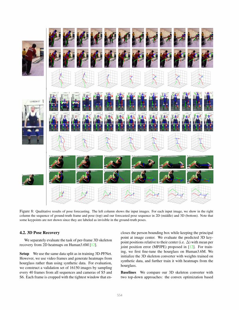
Figure 8: Qualitative results of pose forecasting. The left column shows the input images. For each input image, we show in the right

column the sequence of ground-truth frame and pose (top) and our forecasted pose sequence in 2D (middle) and 3D (bottom). Note that

some keypoints are not shown since they are labeled as invisible in the ground-truth poses.

4.2. 3D Pose Recovery

We separately evaluate the task of per-frame 3D skeleton

recovery from 2D heatmaps on Human3.6M [12].

Setup We use the same data split as in training 3D-PFNet.

However, we use video frames and generate heatmaps from

hourglass rather than using synthetic data. For evaluation,

we construct a validation set of 16150 images by sampling

every 40 frames from all sequences and cameras of S5 and

S6. Each frame is cropped with the tightest window that en-

closes the person bounding box while keeping the principal

point at image center. We evaluate the predicted 3D key-

point positions relative to their center (i.e. ∆) with mean per

joint position error (MPJPE) proposed in [12]. For train-

ing, we first fine-tune the hourglass on Human3.6M. We

initialize the 3D skeleton converter with weights trained on

synthetic data, and further train it with heatmaps from the

hourglass.

Baselines We compare our 3D skeleton converter with

two top-down approaches: the convex optimization based

554

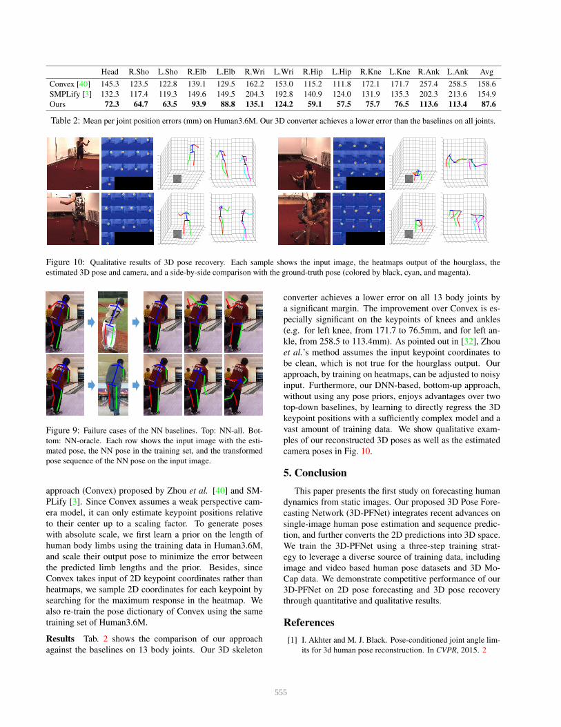
Head R.Sho L.Sho R.Elb L.Elb R.Wri L.Wri R.Hip L.Hip R.Kne L.Kne R.Ank L.Ank Avg

Convex [40] 145.3 123.5 122.8 139.1 129.5 162.2 153.0 115.2 111.8 172.1 171.7 257.4 258.5 158.6

SMPLify [3] 132.3 117.4 119.3 149.6 149.5 204.3 192.8 140.9 124.0 131.9 135.3 202.3 213.6 154.9

Ours 72.3 64.7 63.5 93.9 88.8 135.1 124.2 59.1 57.5 75.7 76.5 113.6 113.4 87.6

Table 2: Mean per joint position errors (mm) on Human3.6M. Our 3D converter achieves a lower error than the baselines on all joints.

−1000 −800 −600 −400 −200 0 200 400 600 800 1000

0

1000

2000

3000

4000

5000

6000

−1500

−1300

−1100

−900

−700

−500

−300

−100

100

300

500 z

y

−1000

0

1000

−1000 −800 −600 −400 −200 0 200 400 600 800 1000

−1000

−800

−600

−400

−200

0

200

400

600

800

1000

zx

y

−1000 −800 −600 −400 −200 0 200 400 600 800 1000

0

1000

2000

3000

4000

5000

6000

−1500

−1300

−1100

−900

−700

−500

−300

−100

100

300

500 z

y

−1000

0

1000

−1000 −800 −600 −400 −200 0 200 400 600 800 1000

−1000

−800

−600

−400

−200

0

200

400

600

800

1000

zx

y

−1000 −800 −600 −400 −200 0 200 400 600 800 1000

0

1000

2000

3000

4000

5000

6000

−1500

−1300

−1100

−900

−700

−500

−300

−100

100

300

500 z

y

−1000

0

1000

−1000 −800 −600 −400 −200 0 200 400 600 800 1000

−1000

−800

−600

−400

−200

0

200

400

600

800

1000

zx

y

−1000 −800 −600 −400 −200 0 200 400 600 800 1000

0

1000

2000

3000

4000

5000

6000

−1500

−1300

−1100

−900

−700

−500

−300

−100

100

300

500 z

y

−1000

0

1000

−1000 −800 −600 −400 −200 0 200 400 600 800 1000

−1000

−800

−600

−400

−200

0

200

400

600

800

1000

zx

y

Figure 10: Qualitative results of 3D pose recovery. Each sample shows the input image, the heatmaps output of the hourglass, the

estimated 3D pose and camera, and a side-by-side comparison with the ground-truth pose (colored by black, cyan, and magenta).

Figure 9: Failure cases of the NN baselines. Top: NN-all. Bot-

tom: NN-oracle. Each row shows the input image with the esti-

mated pose, the NN pose in the training set, and the transformed

pose sequence of the NN pose on the input image.

approach (Convex) proposed by Zhou et al. [40] and SM-

PLify [3]. Since Convex assumes a weak perspective cam-

era model, it can only estimate keypoint positions relative

to their center up to a scaling factor. To generate poses

with absolute scale, we first learn a prior on the length of

human body limbs using the training data in Human3.6M,

and scale their output pose to minimize the error between

the predicted limb lengths and the prior. Besides, since

Convex takes input of 2D keypoint coordinates rather than

heatmaps, we sample 2D coordinates for each keypoint by

searching for the maximum response in the heatmap. We

also re-train the pose dictionary of Convex using the same

training set of Human3.6M.

Results Tab. 2 shows the comparison of our approach

against the baselines on 13 body joints. Our 3D skeleton

converter achieves a lower error on all 13 body joints by

a significant margin. The improvement over Convex is es-

pecially significant on the keypoints of knees and ankles

(e.g. for left knee, from 171.7 to 76.5mm, and for left an-

kle, from 258.5 to 113.4mm). As pointed out in [32], Zhou

et al.’s method assumes the input keypoint coordinates to

be clean, which is not true for the hourglass output. Our

approach, by training on heatmaps, can be adjusted to noisy

input. Furthermore, our DNN-based, bottom-up approach,

without using any pose priors, enjoys advantages over two

top-down baselines, by learning to directly regress the 3D

keypoint positions with a sufficiently complex model and a

vast amount of training data. We show qualitative exam-

ples of our reconstructed 3D poses as well as the estimated

camera poses in Fig. 10.

5. Conclusion

This paper presents the first study on forecasting human

dynamics from static images. Our proposed 3D Pose Fore-

casting Network (3D-PFNet) integrates recent advances on

single-image human pose estimation and sequence predic-

tion, and further converts the 2D predictions into 3D space.

We train the 3D-PFNet using a three-step training strat-

egy to leverage a diverse source of training data, including

image and video based human pose datasets and 3D Mo-

Cap data. We demonstrate competitive performance of our

3D-PFNet on 2D pose forecasting and 3D pose recovery

through quantitative and qualitative results.

References

[1] I. Akhter and M. J. Black. Pose-conditioned joint angle lim-

its for 3d human pose reconstruction. In CVPR, 2015. 2

555

[2] M. Andriluka, L. Pishchulin, P. Gehler, and B. Schiele. 2d

human pose estimation: New benchmark and state of the art

analysis. In CVPR, 2014. 3, 5

[3] F. Bogo, A. Kanazawa, C. Lassner, P. Gehler, J. Romero,

and M. J. Black. Keep it smpl: Automatic estimation of 3d

human pose and shape from a single image. In ECCV, 2016.

2, 8

[4] W. Chen, H. Wang, Y. Li, H. Su, Z. Wang, C. Tu, D. Lischin-

ski, D. Cohen-Or, and B. Chen. Synthesizing training images

for boosting human 3d pose estimation. In 3DV, 2016. 2

[5] R. Collobert, K. Kavukcuoglu, and C. Farabet. Torch7: A

matlab-like environment for machine learning. In BigLearn,

NIPS Workshop, 2011. 5

[6] J. Donahue, L. A. Hendricks, S. Guadarrama, M. Rohrbach,

S. Venugopalan, T. Darrell, and K. Saenko. Long-term recur-

rent convolutional networks for visual recognition and de-

scription. In CVPR, 2015. 1

[7] Y. Du, Y. Wong, Y. Liu, F. Han, Y. Gui, Z. Wang, M. Kankan-

halli, and W. Geng. Marker-less 3d human motion capture

with monocular image sequence and height-maps. In ECCV.

2016. 2

[8] C. Finn, I. Goodfellow, and S. Levine. Unsupervised learn-

ing for physical interaction through video prediction. In

NIPS. 2016. 2

[9] K. Fragkiadaki, S. Levine, P. Felsen, and J. Malik. Recurrent

network models for human dynamics. In ICCV, 2015. 1, 2

[10] G. Gkioxari, A. Toshev, and N. Jaitly. Chained predictions

using convolutional neural networks. In ECCV, 2016. 2

[11] K. He, X. Zhang, S. Ren, and J. Sun. Deep residual learning

for image recognition. In CVPR, 2016. 3

[12] C. Ionescu, D. Papava, V. Olaru, and C. Sminchisescu.

Human3.6m: Large scale datasets and predictive methods

for 3d human sensing in natural environments. TPAMI,

36(7):1325–1339, July 2014. 5, 7

[13] Y. Jia, E. Shelhamer, J. Donahue, S. Karayev, J. Long, R. Gir-

shick, S. Guadarrama, and T. Darrell. Caffe: Convolu-

tional architecture for fast feature embedding. arXiv preprint

arXiv:1408.5093, 2014. 6

[14] R. Jozefowicz, W. Zaremba, and I. Sutskever. An empiri-

cal exploration of recurrent network architectures. In ICML,

2015. 3

[15] T. Lan, T.-C. Chen, and S. Savarese. A hierarchical repre-

sentation for future action prediction. In ECCV, 2014. 2

[16] S. Li and A. B. Chan. 3d human pose estimation from

monocular images with deep convolutional neural network.

In ACCV, 2014. 2

[17] M. Mathieu, C. Couprie, and Y. LeCun. Deep multi scale

video prediction beyond mean square error. In ICLR, 2016.

1, 2

[18] R. Mottaghi, H. Bagherinezhad, M. Rastegari, and

A. Farhadi. Newtonian image understanding: Unfolding the

dynamics of objects in static image. In CVPR, 2016. 2

[19] A. Newell, K. Yang, and J. Deng. Stacked hourglass net-

works for human pose estimation. In ECCV, 2016. 2, 3, 4,

6

[20] B. X. Nie, C. Xiong, and S. C. Zhu. Joint action recognition

and pose estimation from video. In CVPR, 2015. 2

[21] S. L. Pintea, J. C. van Gemert, and A. W. M. Smeulders. Deja

vu: Motion prediction in static images. In ECCV, 2014. 1, 2

[22] G. Rogez and C. Schmid. Mocap-guided data augmentation

for 3d pose estimation in the wild. In NIPS. 2016. 2

[23] Z. Shou, D. Wang, and S.-F. Chang. Temporal action local-

ization in untrimmed videos via multi-stage cnns. In CVPR.

2016. 1

[24] K. Simonyan and A. Zisserman. Two-stream convolutional

networks for action recognition in videos. In NIPS. 2014. 1

[25] N. Srivastava, E. Mansimov, and R. Salakhutdinov. Unsu-

pervised learning of video representations using lstms. In

ICML, 2015. 1, 2

[26] B. Tekin, I. Katircioglu, M. Salzmann, V. Lepetit, and P. Fua.

Structured prediction of 3d human pose with deep neural net-

works. In BMVC, 2016. 2

[27] J. J. Tompson, A. Jain, Y. LeCun, and C. Bregler. Joint train-

ing of a convolutional network and a graphical model for

human pose estimation. In NIPS. 2014. 2

[28] C. Vondrick, H. Pirsiavash, and A. Torralba. Generating

videos with scene dynamics. In NIPS. 2016. 2, 3

[29] J. Walker, C. Doersch, A. Gupta, and M. Hebert. An uncer-

tain future: Forecasting from static images using variational

autoencoders. In ECCV, 2016. 1, 2, 3

[30] J. Walker, A. Gupta, and M. Hebert. Patch to the future:

Unsupervised visual prediction. In CVPR, 2014. 1, 2

[31] J. Walker, A. Gupta, and M. Hebert. Dense optical flow pre-

diction from a static image. In ICCV, 2015. 1, 2

[32] J. Wu, T. Xue, J. J. Lim, Y. Tian, J. B. Tenenbaum, A. Tor-

ralba, and W. T. Freeman. Single image 3d interpreter net-

work. In ECCV, 2016. 2, 3, 4, 8

[33] T. Xue, J. Wu, K. L. Bouman, and W. T. Freeman. Visual

dynamics: Probabilistic future frame synthesis via cross con-

volutional networks. In NIPS. 2016. 2

[34] J. Yang, S. E. Reed, M.-H. Yang, and H. Lee. Weakly-

supervised disentangling with recurrent transformations for

3d view synthesis. In NIPS. 2015. 4

[35] Y. Yang and D. Ramanan. Articulated human detection with

flexible mixtures of parts. TPAMI, 35(12):2878–2890, Dec

2013. 5

[36] H. Yasin, U. Iqbal, B. Kruger, A. Weber, , and J. Gall. A

dual-source approach for 3d pose estimation from a single

image. In CVPR, 2016. 2

[37] S. Yeung, O. Russakovsky, G. Mori, and L. Fei-Fei. End-

to-end learning of action detection from frame glimpses in

videos. In CVPR. 2016. 1

[38] J. Yuen and A. Torralba. A data-driven approach for event

prediction. In ECCV, 2010. 1, 2

[39] W. Zhang, M. Zhu, and K. G. Derpanis. From actemes to

action: A strongly-supervised representation for detailed ac-

tion understanding. In ICCV, 2013. 5

[40] X. Zhou, S. Leonardos, X. Hu, and K. Daniilidis. 3d shape

estimation from 2d landmarks: A convex relaxation ap-

proach. In CVPR, 2015. 2, 3, 8

[41] X. Zhou, M. Zhu, S. Leonardos, K. G. Derpanis, and

K. Daniilidis. Sparseness meets deepness: 3d human pose

estimation from monocular video. In CVPR, 2016. 2

556