forecasting foreign exchange rates: a comparative evaluation of ahp
TRANSCRIPT

Pergamon
Omega, Int. J. Mgmt Sci. Vol. 22, No. 5, pp. 505-519, 1994 Copyright !¢! 1994 Elsevier Science Ltd
0305-0483(94)00028-X Printed in Great Britain. All rights reserved 0305-0483/94 $7.00 + 0.00
Forecasting Foreign Exchange Rates: A Comparative Evaluation of AHP
F 13LENGIN
B ULENGIN
Istanbul Technical University, Turkey
(Received July 1993; accepted after revision April 1994)
In the first part of this paper the US DollarlDM exchange rates for two different time periods are forecast based on the analytical hierarchy process using the judgements of five experts. Then, the same forecasting activity is repeated via classical approaches namely Regression Analysis, ARIMA Modelling, VAR, Restricted VAR (RVAR) and Bayesian VAR (BVAR). Finally, the forecasting accuracy of the methods are compared and the results are evaluated.
Key words--forecasting, foreign exchange, AHP, ARIMA, VAR, regression
INTRODUCTION
CLASSICAL METHODS used to forecast the financial market phenomena, generally have several draw- backs. First of all, they forecast the future based solely on past data. For example, econometric models do not integrate qualitative and non- quantifiable parameters such as the behaviour of relevant actors. Classical models are both deterministic and structurally stable, which leads to error in forecasting. They do not take into account the possible changes in trends and include a few explanatory variables, most of which are easily quantified. They also usually assume that economic, social and political forecasts are independent of each other.
Nowadays there is a tendency to accept that market analysts' and other experts' intervention can realize more accurate forecasts [5]. Unfor- tunately, however, there are only a few studies describing the process by which experts can integrate their knowledge to realize that forecast [2, 3, 10, 19]. Saaty and Vargas's research [26, pp. 141-151] is one of them. It is concerned with forecasting the value of the Yen/US Dollar
exchange rate but is based solely on the applica- tion of the Analytic Hierarchy Process (AHP). It claims, without any relative comparison, that the AHP framework will allow the incorporation of current market knowledge and expertise to generate a subjective probability distribution of the future spot rate and, thus, provide more accurate probabilities than the conventional forecasting approaches which can not accom- plish this directly. This paper aims to investigate the relevance of this claim. The study concerns the forecast of the future value of the US Dollar/ DM exchange rate for the monthly average of April and December 1993.
The study is based on empirical comparisons of the AHP with classical forecasting methods with respect to their 3-month ahead forecasting power. In order to get an accurate comparison, at the first stage the monthly average of April 1993 is forecast on January 1993 and then the same analysis is repeated on September 1993 to forecast the monthly average of December 1993. Besides the AHP procedure, Box-Jenkins ARIMA modelling, Regression Analysis, VAR, Bayesian VAR (BVAR) and Restricted VAR
505

506 ~llengin, ~llengin--Comparative Evaluation of AHP
(RVAR) are used for the same purpose and their results are compared to analyse whether Saaty and Vargas's claim can be proven or not.
ANALYTIC HIERARCHY PROCESS
The AHP is an intuitive and relatively easy method for formulating and analysing decisions. It structures the decision problem in levels which correspond to one's understanding of the situation; goal, criteria, sub-criteria and altern- atives. By breaking the problem into levels, the decision maker can focus on smaller sets of decisions. The overall philosophy of the AHP is to provide a solid, scientific method to aid in the creative formulation of a decision problem. The method is based on the elicitation of priorities for a given set of alternatives A under a given criterion c ~ C which involves the completion of an n x n matrix, where n is the number of alternatives under consideration. However, since the comparisons are assumed to be reciprocal, one needs to make only n (n - 1)/2 of the com- parisons to fill in the matrix of judgements, com- pletely. This matrix A is positive and symmetric.
The first and simplest method to derive the overall ranking of the alternatives from the pairwise comparisons is simply to normalize one column. However, when errors are permitted in eliciting the pairwise comparisons, the final answer will depend on which column is chosen for the normalisation. Saaty proposes an eigen- vector approach for the estimation of weights from a matrix of pairwise comparisons [25]. After generating a set of weights w,,, for each alternative a e A under criterion c e C, the principle of hierarchical composition provides a way of computing the overall priority of the alternatives by summing the priority under criterion c times the priority of criterion c:
W a = ~ Vc • Wac ¢
As can be seen from the formula, a linear additive function is used to represent the composite priorities of alternatives.
THE EXCHANGE RATE AHP-BASED FORECASTING FRAMEWORK
Based upon existing theories of foreign exchange rate determination as well as upon the identification of the expert group, a set of
factors concerning the exchange rate forecasting framework is determined. In this study, the expert group consisted of five experts: three professors who teach and research in the areas of International Economics and International Finance and two experts from the Banking Sector. Five primary indicators of future exchange rate are identified: Relative Interest Rates (RIR), Official Exchange Market Inter- vention (OFMI), Relative Degree of Confidence in the US Economy (RDC), the US Current Account Balance (CAB) and the Past Behaviour of Exchange Rates (PBEX). In fact, those factors were similar to those suggested by Saaty and Vargas [26, pp. 141-151] with the exception that the latter also incorporated the Foreign Exchange Bias Factor into the analysis. How- ever, the relative priority of this is found to be of little importance by our experts and, thus, excluded from consideration.
Relative Interest Rates ( R I R )
This factor is intended to investigate the impact of the interest rate differentials between American and German financial centers on the exchange rate changes. For example, if interest rates in Germany rise relative to world rates, the demand for DM-dominated assets will increase and, thus, result in an increasing demand for DM in the foreign exchange market. Three sub-factors (at the third level) are accepted to exist under this cluster; namely the Monetary Policy of the US Federal Reserve (USMP), the Monetary Policy of the Bank of Germany (GMP) and the Size of the US Federal Budget Deficit (SFD). The fourth level of the hierarchy provides evaluations of the likely directions of these sub-factors. The first two sub-factors were assigned three indicators--tighter, steady and easier--while the third was evaluated on its relative likelihood of contracting, stabilizing or expanding. As will be shown later, based on the pairwise comparison matrices reflecting the judgements of experts, the relative probability of each of them was specified. At the fifth level, the probable impact of each of these indicators on the future value of the exchange rate was evaluated using a set of arbitrary ranges. Sharp Decline, Moderate Decline, No Change, Sharp Increase and Moderate Increase were used as possible characterization of this future value.
The midpoint of No Change range for US Dollar/DM exchange rate is the value of

Omega, Vol.
January 1993 for the first period evaluation and that of September 1993 for the second period evaluation. The length of No Change zone is one standard deviation of the parity and the latter is calculated based on the last 12 months. Subsequently, the area beyond two standard deviation is taken to be the Sharp Increase (Decrease) range while the area in between is called the Moderate Increase (Decrease) range. The value of the limits corresponding to those ranges for both the first and second period evaluations are given in Table 15.
O Ofcial Exchange Market Intervention (OFMI)
The Central Bank intervention is another factor accepted to influence the foreign exchange markets. In fact, different points of view exist on this subject. Some experts suggest that the impact of a reasonable intervention will not be so great while others believe that by signalling a change in the policy, it may greatly affect expectations. At the third level of the hierarchy, this intervention was accepted as being of either consistent (CONS) or erratic (ERRAT). The fourth level shows that a consistent or erratic intervention may be strong, moderate or weak and judgements were made concerning the likelihood of each.
Relative Degree of Confidence in the US economy (RDC)
Investor confidence in the relative economic and political stability was accepted to be one of the indicators of the future value of the exchange rate. An increase or decrease in confidence could result in significant revisions in expenditure and investment strategies. At the third level, three sub-factors; namely Relative Rate of Inflation (RINFR), Relative Real Growth (RRGWTH) and Relative Political Stability (RPOLST) were utilised as the deter- minations of this second level element. On the fourth level, for the first two, the likelihood of being higher, equal or lower (in the US) and for the relative political stability variable, the likeli- hoods of being more, equally or less stable were assessed.
Current Account Balance (CAB)
The countries' current account balances were also accepted as important indicators. For example, an unanticipated change in the current account may provide new information about
22, No. 5 507
shifts in terms of trade, which most probably leads to a change in the exchange rate. There- fore, more accurate information about the current account can be used to forecast forth- coming changes in the exchange rate. The Size of the Deficit or Surplus (SDEFS) and Antici- pated Changes (ANCH) in the balance were accepted to be the two, third level sub-factors summarising the impact of the current account balance. On the fourth level, large and small were accepted to be the two determinants of the size of deficit or surplus and decrease. No change and increase were taken as the indicators of the anticipated changes.
Past Behaviour of Exchange Rates (PBEX)
The AHP framework used in this paper, also accepts the incorporation of PBEX into the analysis as information predictive of the future exchange rate. The third level categorises factors according to the relevance (REL) and irrelevance (IRRL) of historical data. On the fourth level, each category is further designated as having high, medium or low explanatory power.
Figure 1 gives the final US Dollar/DM Exchange Rate Forecasting Hierarchy derived from the judgements.
EVALUATION OF THE FIRST PERIOD JUDGEMENTS BASED ON AHP
According to the first period evaluation made in January 1993, the relative and composite priorities of all the factors affecting the 3-month ahead average of US Dollar/DM exchange rate are presented in Tables 1-4. In all, there were 43 matrices of paired comparisons for each expert, each based on n(n - 1)/2 judgements. In order to reach the group decision results, for each pairwise comparison matrix, the geometric mean of the individual evaluations is taken.
Based on the relative priorities obtained as a result of these paired comparisons, the most important second level factors accepted to affect
Table I. Relative and composite priorities of level 2 for the first period evaluation
Relative Composite Level 2 factors impact priority
RIR I 0.3626 0.3626 OFMI II 0.0451 0.0451 RDC Ill 0.1850 0.1850 CAB IV 0.2861 0.2861 PBEX V 0.1212 0.1212

508 Olengin, Olengin--Comparative Evaluation t~]" AHP )Va° I exchange rate
in 90 days
r/l D
I. Tighter, Steady, Easier 2. Tighter, Steady, Easier 3. Contract , No change, Expand 4. Strong, Moderate, Weak 5. Higher, Equal, Lower 6. Higher, Equal, Lower 7. More, Equally, Less stable 8. Large, Small 9. Decrease, No change, Increase 10. High, Medium, Low 11. High, Medium, Low
Fig. 1. D o l l a r / M a r k e x c h a n g e ra te fo recas t ing h ie ra rchy .
the exchange rate were the RIR differentials (0.3626) and CAB (0.2861). The third important factor was judged to be RDC in the US (0.185), and the fourth was PBEX (0.1212). OFMI
(0.0451) was held to be of rather minor signifi- cance for this particular 3-month forecasting problem (Table 1). In fact, it is necessary to underline that these priorities could change with
Com. Pri.
6. USMP 7. GMP 8. SFD
9. CONS 10. ERRAT
I 1. RINFR 12. RRGWTH 13. RPOLST
14. SDEFS 15. ANCH
16. REL 17. IRREL
Table 2. Relative and composite priorities of level 3 for the first period evaluation
RIR OFMI RDC CAB PBEX I II 1II IV V
0.3626 0.0451 0.1850 0.2861 0.1212
0.4286 0.4286 0.1428
0.5973 0.2824 0.1203
0.8333 0.1667
0.8333 0.1667
0.8330 0.1670
Comp. Pri. Renorm. Pri.
0.1554 0.1566 0.1554 0.1566 0.0518 0.0522
0.0376 0.0379 7.52 × 10 3.
0.1105 0.1113 0.0522 0.0526 0.0223 0.0223
0.2384 0.2402 0.0477 0.0481
0.1010 0.1018 0.0202 0.0204
*Omitted from further consideration.

Tab
le 3
. R
elat
ive
and
com
posi
te p
rior
ities
o
flev
el4
fort
he
firs
t pe
riod
eva
luat
ion
US
MP
G
MP
S
FD
O
FM
I R
INF
R
RR
GW
TH
R
PO
LS
T
SD
EF
S
AN
CH
R
EL
IR
RL
6
7 8
9 11
12
13
14
15
16
17
C
omp.
Pr.
R
en.
Co
m.
Pr.
0.15
66
0.15
66
0.05
22
0.03
79
0.11
13
0.05
26
0.02
23
0.24
02
0.04
81
0.10
18
0.02
04
0.08
06
0.01
26
0.01
33
0.58
70
0.09
19
0.09
65
0.33
24
0.05
2 0.
0546
0.10
91
0.11
46
0.03
63
0.03
81
0.01
12
0.01
18
0.05
51
2.88
x 1
0 3,
0.
2162
0.
0113
0.
0113
0.
7287
0.
038
0.03
99
18.
Tig
hter
19
. S
tead
y 20
. E
asie
r
21.
Tig
hter
22
. S
tead
y 23
. E
asie
r
24.
Con
trac
t 25
. N
o C
hang
e 26
. E
xpan
d
27.
Str
ong
28.
Mo
der
ate
29.
Wea
k
33.
Hig
her
34.
Equ
al
35.
Low
er
36.
Hig
her
37.
Equ
al
38.
Low
er
39.
Hig
her
40.
Equ
al
41.
Low
er
42.
Lar
ge
43.
Smal
l
44.
Dec
reas
e 45
. N
o C
hang
e 46
. In
crea
se
47.
Hig
h 48
. M
ediu
m
49.
Low
50.
Hig
h 51
. M
ediu
m
52.
Low
4 x
10
3,
0.02
4 9.
9 x
10
3,
0.07
0.
0289
0.
0118
6.3
x 10
3,
0.
0148
0.
0314
6.3
x 10
3,
0.
0133
2.
7 x
10
3,
0.2
0.04
0.01
0.
0327
4.
9 x
10
3,
0.02
15
0.06
99
0.01
04
2.4
x 10
-3*
6.7
x 10
-3*
0.01
1
0.69
65
0.23
16
0.07
19
0.10
62
0.63
33
0.26
05
0.63
33
0.26
05
0.10
62
0.12
03
0.28
24
0.59
73
0.28
24
0.59
73
0.12
03
0.83
33
0.16
67
0.21
14
0.68
64
0.10
22
0.21
14
0.68
64
0.10
22
0.11
96
0.33
12
0.54
92
0.02
5
0.07
35
0.03
03
0.01
24
0.01
55
0.03
3
0.01
4
0.21
0.
042
0.01
1 0.
0343
0.02
26
0.07
34
0.01
09
0.01
7

510 Olengin, ~llengin--Comparative Evaluation of AHP
Table 4. Relative and composite priorities of level 5 for the first period evaluation
Com. Pri. Sharp Decrease Moderate Decrease No Change Moderate Increase Sharp Increase
USMP 18. Tighter 0.0133 0.2157 0.1081 0.0595 0.1371 0.4796 19. Steady 0.0965 0.0836 0.0634 0.3302 0.3863 0.1365 20. Easier 0.0546 0.1499 0.1448 0.5104 0.1493 0.0456
GMP 21. Tighter 0.1146 0.4437 0.1351 0.0454 0.1039 0.2719 22. Steady 0.0381 0.2427 0.1170 0.3670 0.1650 0.1083 23. Easier 0.0118 0.0722 0.2200 0.4905 0.1587 0.0586
SFD 25. No Change 0.0113 0.3267 0.1277 0.1510 0.2298 0.1648 26. Expand 0.0399 0.3487 0.1538 0.0421 0.2277 0.2277
OFMI 28. Moderate 0.025 0.3269 0.1598 0.1045 0.2387 0.1701
RINFR 33. Higher 0.0735 0.4369 0.2766 0.0418 0.0858 0.1589 34. Equal 0.0303 0.0705 0.1291 0.5422 0.2101 0.0481 35. Lower 0.0124 0.0712 0.1847 0.3767 0.2652 0.1022
RRGWTH 37. Equal 0.0155 0.0639 0.3932 0.3137 0.1415 0.0877 38. Lower 0.033 0.1026 0.1645 0.4164 0.2434 0.0731
RPOLST 40. Equal 0.014 0.0859 0.1585 0.5146 0.1916 0.0494
SDEFS 42. Large 0.21 0.1855 0.0966 0.0677 0.2386 0.4116 43. Small 0.042 0.1686 0.314 0.1493 0.2649 0.1032
ANCH 44. Decrease 0.011 0.2391 0.0952 0.3218 0.2166 0.1273 45. No Change 0.0343 0.0533 0.1602 0.4988 0.1977 0.09
REL 47. High 0.0226 0.1026 0.2434 0.1645 0.4164 0.0731 48. Medium 0.0734 0.0637 0.299 0.1089 0.3726 0.1558 49. Low 0.0109 0.1172 0.1484 0.2582 0.3651 0.111
IRRL 52. Low 0.012 0.1142 0.1538 0.4473 0.2142 0.0705
respect to time horizon and different exchange rate institutional arrangements.
The analyses of the relative priorities for the lower factors shows that both USMP and GMP (0.4286 and 0.4286 respectively) are the primary factors affecting RIR (Table 2). The first one was tending to be steady (0.587) and the second one was judged to be tending toward greater tightness (0.6965) (Table 3). Other things being equal, it was assessed that the steadiness of the USMP would either produce stabilization (0.3302) or a moderate increase (0.3863) at the current exchange rate. On the other hand, the tightness of the GMP would result in a sharp decline (0.4437) (Table 4).
A second interpretation could be realized for the CAB which was judged to be influenced mostly by the SDEFS (0.8333) (Table 2), the latter tending to be large (0.8333) in the next 3-month period (Table 3). Other things being equal, it was assessed that this would most probably result in a sharp increase (0.4116) at the current exchange rate (Table 4).
As another example, the most important factor affecting the RDC in the US was judged to be RINFR (0.5973) (Table 2) which was expected to be higher (0.6333) (Table 3) in the next 3-month period. Other things being equal, this would result in a sharp decline (0.4369) at the current exchange rate (Table 4).
Further judgements were made for the PBEX (0.8333) (Table 2) but this relevancy, which was judged to be of medium degree (0.6864) (Table 3), would most probably lead to a moderate (0.3726) or sharp (0.1558) increase (Table 4) at the current exchange rate. Finally, OFMI, which was found to be of minor import- ance in affecting the rates, was also thought to be consistent (0.8333) (Table 2) at a moderate level (0.6333) (Table 3). Other things being unchanged, this would result in a sharp (0.3269) or moderate (0.1598) decline (Table 4) at the current exchange rate.
The right-hand side column of Tables 1-4 give the composite priorities which show the impact of importance of each factor and sub-

Omega, Vol.
Table 5. Probability distribution of US Dollar/DM outcome ranges for the first period evaluation
Cumulative Scenarios Probability probability
Sharp Decline 0.2067 0.2067 Moderate Decline 0.1608 0.3675 No Change 0.2425 0.5700 Moderate Increase 0.2275 0.7975 Sharp Increase 0.2025 1.0000
22, No. 5 511
Table 6. Relative and composite priorities of level 2 for the second period evaluation
Relative Composite Level 2 factors impact priority
RIR I 0.4942 0.4942 OFMI II 0.0787 0.0787 RDC III 0.2564 0.2564 CAB IV 0.1458 0.1458 PBEX V 0.0249 0,0249
factor on the value of the Dollar/DM exchange rate. In fact, those values are computed by multiplying the relative priority of each by the relative priority of the higher level factor to which they belong.
The pairwise comparisons of this first period judgements showed that the probability of an erratic market intervention was very unlikely (7.52 x 10 -3) and, thus, was omitted from further consideration. A similar case was that of the higher relative real growth (6.3 x 10 -3) and less stable (2.7 x 10 -3) political structure as well as the high (2.4 x 10 -3) or medium (6.7 x 10 -3) explanatory power of an irrelevant historical data and an increase as an anticipated change (4.9 x 10⁻³).
Based on these results, it could be said that as a third level factor, the SDEFS would have the highest composite priority (0.2402) while the USMP (0.1556) and the GMP (0.1556) would be ranked second in importance (Table 2). Further- more, the largeness of the SDEFS (0.21) and the tendency toward greater tightness of the GMP (0.1146) were judged to have the greatest com- posite priorities on the fourth level (Table 3). Similarly, the composite priorities (subjective set of weights) of the lowest level of the hierarchy were computed. Table 5 presents the subjective set of weights for these ranges. Figures to the right are the cumulative priorities. According to
the relative priorities, the No Change range had the highest probability of occurring (0.2425) and, thus, ranked first while a Moderate Increase (0.2275) was found to have the second priority.
EVALUATION OF THE SECOND PERIOD JUDGEMENTS BASED ON THE AHP
When the same analysis was repeated in September 1993 to forecast the average exchange rate of December 1993, with the same expert group, the experts' pairwise comparisons showed that the most important second level factor affecting the exchange rate for the new period under consideration was RIR differential (0.4942) as before but its degree of importance was relatively (0.3626 for the first period) greater. The second important factor was judged to be RDC in the US (0.2564) and the third was the CAB (0.1458). The OFMI and PBEX were found to be rather insignificant for this particular period under consideration (Table 6).
The analyses of the relative priorities of the lower level factors given at Table 7 showed that the primary factors affecting RIR was thought to be USMP (0.5893) while GMP was ranked second in importance (0.2589). Both were judged to be tending toward steadiness (0.6017 and 0.547 respectively) (Table 8). Additionally, in the ceteris paribus conditions, the judgements
Table 7, Relative and composite priorities of level 3 for the second period evaluation
RIR OFMI RDC CAB PBEX I lI In IV v Comp. Pri. Renorm. Pri.
0.4942 0.0787 0.2564 0.1458 0.0249
0.5893 0.2912 0.3017 0.2589 0.1279 0.1325 0.1518 0.0750 0.0777
0.0689 0.0714 9.8 x I0 3,
0.6965 0.1786 0.1850 0.2316 0.0594 0.0615 0.0719 0.0184 0.0191
0.8888 0.1296 0.1343 0.1112 0.0162 0.0168
4.15 x 10 3, 0.02 x 10 3*
Priority
6. USMP 7. GMP 8. SFD
9. CONS 10. ERRAT
1 I. RINFR 12. RRGWTH 13. RPOLST
14. SDEFS 15, ANCH
16. REL 17. IRRL
0.8750 0.1250
0.1667 0.8333

t,O
Tab
le 8
. R
elat
ive
and
com
posi
te p
rior
itie
s o
flev
el4
fort
he
firs
t p
erio
dev
alu
atio
n
US
MP
G
MP
S
FD
O
FM
I R
INF
R
RR
GW
TH
R
PO
LS
T
SD
EF
S
AN
CH
6
7 8
9 II
12
13
14
15
C
om
p.
Pr.
R
enor
m.
Pfi
.
0.30
17
0.13
25
0.07
77
0.07
14
0.18
50
0.06
15
0.01
91
0.13
43
0.01
68
0.27
69
0.08
35
0.08
64
0.60
17
0.18
15
0.18
78
0.12
14
0.03
66
0.03
79
0.O
436
0.04
51
0.07
25
0.07
5 0.
0164
0.
0169
0.07
19
5.59
x 1
0 3,
0.
2316
0.
018
0.01
86
0.69
65
0.05
41
0.05
59
8.59
x 1
0 -3
* 0.
0202
0.
0426
18.
Tig
hter
19
. S
tead
y 20
. E
asie
r
21.
Tig
hter
22
. S
tead
y 23
. E
asie
r
24.
Con
trac
t 25
. N
o C
hang
e 26
. E
xpan
d
27.
Str
ong
28.
Mod
erat
e 29
. W
eak
30.
Str
ong
31.
Mo
der
ate
32.
Wea
k
33.
Hig
her
34.
Equ
al
35.
Low
er
36.
Hig
her
37.
Equ
al
38.
Low
er
39.
Hig
her
40.
Equ
al
41.
Low
er
42.
Lar
ge
43.
Sm
all
44.
Dec
reas
e 45
. N
o C
hang
e 46
. In
crea
se
0.32
94
0.54
70
0.12
36
0.12
03
0.28
24
0.02
09
0.59
73
0.04
41
0.13
07
0.19
25
0.67
68
0.60
33
0.28
53
0.11
14
0.64
34
0.28
28
0.07
38
0.14
29
0.85
71
0.66
7 0.
1504
0.
1826
0.02
42
0.02
51
0.03
56
0.03
68
0.12
52
0.12
96
0.03
7 0.
0384
0.
0175
0.
0182
6.
85 x
10
3,
0.01
23
0.01
27
5.4
× 1
0 -3
* 1.
4 x
10 -3
*
0.01
92
0.01
99
0.11
51
0.11
91
0.01
12
0.01
16
2.53
x 1
0 3,
3.
07 x
10 -
3*
I t~
*Om
itte
d fr
om f
urth
er c
onsi
dera
tion
.

Omega, Vol. 22, No. 5
Table 9. Relative and composite priorities of level 5 for the second period evaluation
513
Comp. Pri. Sharp Decrease Moderate Decrease No Change Moderate Increase Sharp Increase
USMP 18. Tighter 0.0864 0.0836 0.1883 0.2801 0.4061 0.0419 19. Steady 0.1878 0.0337 0.1150 0.2711 0.5131 0.0671 20. Easier 0.0379 0.0409 0.5604 0.1388 0.1686 0.0913
GMP 21. Tighter 0.0451 0.1800 0.1057 0.1326 0.3793 I).2024 22. Steady 0.075 0.0343 0.1413 0.5635 0.2032 0.0577 23. Easier 0.0169 0.1037 0.0947 0.1336 0.4921 0.1759
SFD 25. No Change 0.0186 0.0539 0.1697 0.2090 0.4081 0.1593 26. Steady 0.0559 0.2702 0.4015 0.1681 0.1193 0.0409
OFM I 28. Moderate 0.0209 0.1214 0.2568 0.0579 0.4638 0.1001 29. Weak 0.0441 0.0513 0.2760 0.2818 0.3185 0.0724
RINFR 33. Higher 0.0251 0.4891 0.2743 0.1335 0.0769 0.0262 34. Equal 0.0368 0.0472 0.1843 0.5746 0.1618 0.0327 35. Lower 0.1296 0.5008 0.2605 0.1413 0.0694 0.028
RRGWTH 36. Higher 0.0384 0.034 0.0868 0.1 0.5026 0.2766 37. Equal 0.0182 0.0426 0.1473 0.5612 0.1954 0.0535
RPOLST 39. More stable 0.0127 0.1028 0.4615 0.1027 0.2403 0.0927
SDEFS 42. Large 0.0199 0.1032 0.1458 0.0858 0.4702 0.195 43. Small 0.1191 0.0659 0.1751 0.3072 0.3649 0.0869
ANCH 44. Decrease 0.0116 0.1436 0.5124 0.2367 0.0776 0.0297
underline that the steadiness of USMP would, most probably, produce a Moderate Increase (0.5131) or No Change (0.2711) and the steadi- ness of the GMP would, most likely, produce stabilization (0.5635) (Table 9).
The same type of interpretations may be repeated for the other factors. For example RDC in US which was found to be the second most important factor (0.2564) (Table 6) influencing the exchange rate was mostly influenced by the RINFR (0.6965) (Table 7) which is expected, in its turn, to be lower (0.6768) (Table 8) in the period under consideration. Other things held constant, this would, most probably, result in a Sharp Decline (0.5008) of the relative exchange rate (Table 9). Similarly, the element which has the greatest impact on the third important second level factor (CAB) was found to be SDEFS (0.8888) (Table 7) expected to be small (0.8571) (Table 8) for the period under consider- ation and this alone was judged to result in either No Change (0.3072) or Moderate Increase (0.3649) (Table 9).
When the composite priorities are calculated at each level, in a manner similar to that of the first period evaluations, those of minor import- ance are omitted from consideration and the remaining ones are renormalized to be used in
the subsequent tables. An example to this is the omittment of an erratic exchange rate inter- vention (9.84 × 10 -3) as well as the relevance (4.15 x l0 -3) and irrelevancy (0.02 x l0 -3) of past behaviour corresponding to the third level evaluations (Table 7).
Consequently, based on these calculations, it was found that USMP has the highest com- posite priority (0.3017) as a third level factor while RINFR is ranked second in importance (0.185) concerning the composite influence on the relative exchange rate (Table 7).
Those results are slightly different from the first period evaluations (Table 2) where SDEFS had the highest priority (0.2402) and the USMP (0.1556) and of the GMP (0.1556) were ranked second in importance. Subsequently, at the fourth level, the steadiness of the USMP (0.1878) and the lower level of the RINFR (0.1296) were judged to have the greatest composite priorities (Table 8).
As a final step, based on the significant (i.e. not omitted) composite priorities of the fourth level factors, which reflect, in fact, their subjective set of weights, the composite priorities of the lowest level factors are computed. The resulting values reflect the subjective weights corresponding to possible ranges of the relative

514 Olengin, Olengin--Comparative Evaluation of AHP
Table 10. Probability distribution of US Dollar/DM outcome ranges for the second period evaluation
Cumulative Scenarios Probability probability
Sharp Decline 0.1423 0.1423 Moderate Decline 0.2082 0.3505 No Change 0.2570 0.6075 Moderate Increase 0.3130 0.9205 Sharp Increase 0.0795 1.0000
exchange rate. According to the first figures given in the table, Moderate Increase got the highest composite priority (0.313) while No Change was ranked as the second possibility (0.257) (Table 10). Figures on the right give the cumulative probabilities.
THE EXCHANGE RATE CONVENTIONAL FORECASTING FRAMEWORK
Since this study was concerned with the forecasting of the US Dollar/DM parity, we compared the regression (economic theory based) methods and time-series methods. The regression forecast was based on a causal model. As alternatives to the regression model, the autoregressive integrated moving average (ARIMA) model, as proposed by Box and Jenkins [6], VAR, Bayesian VAR (BVAR) and Restricted VAR (RVAR) models were con- structed. The details of their formulations are given in Appendix A.
For many decades of applied macroecon- omics, the prevailing response to the challenge of how to combine abstract theoretical reasoning with inference from economic data has consisted of building and estimating detailed macroecon- omic models. However, Sims criticizes building up large structural econometric forecasting models, equation by equation [27]. Of special concern to Sims are the often arbitrary exclusion restrictions used to identify the models.
As an alternative to structural econometric models, the univariate ARIMA model has been quite successful in time-series forecasting. The main problem with the ARIMA model is its failure to consider information about other potentially important variables. Vector auto- regression (VAR) models represent one approach toward incorporating this information. However, some do not forecast well [20, 23].
The use of a theoretical VAR model is a powerful tool for empirical model building because (1) the procedure avoids imposing incredible identifying solutions, (2) the estima-
tion procedure is simple and consistent and (3) the significance of explanatory variables offers a causality test in the spirit of Wiener and Granger. In terms of the traditional econometric literature, a multivariate time-series model provides a fairly unrestricted approximation to the reduced form of some unknown structural system of simulataneous equations. Lupoletti and Webb [22], Funke [12, 13], Holden and Broomhead [16], Baghestani and McNown [4], Chishti et al. [7] and Literman [21] argue that VAR models can produce forecasts that are at least competitive with large scale structural models. Some researchers have argued that changing a model slightly can produce signifi- cantly different results [18, 24, 30]. On the other hand, Sims has refuted these claims [28, 29]. In short, neither its robustness nor the opposite are proven. Todd objectively examined both sides of the debate [33].
The first forecasting alternative considered was the traditional econometric approach and the causal model was based on economic theory. The asset market approach to exchanges rates determination views the exchange rate as the price of international assets that adjusts, to clear the relative demand and supply of domestic and foreign assets. According to the asset market approach the exchange rate must adjust instantaneously to equilibrate the international demand for stocks of national assets.
The monetary approach to exchange rates states that the exchange rates is the price of foreign currency and as any other relative price, the exchange rate is determined by relative demand and supply of two moneys. This leaves the monetary markets as the main determinants of exchange rates. This branch of asset market approach views the exchange rates as equi- librating domestic and foreign money markets. A detailed review of the models can be found at [34].
In this study, none of the explained approaches are directly used to specify the regression equation. The general to simple methodology is used to specify equations. This approach starts with a very general hypothesis that is acceptable to all the economists and then narrows it down by looking for simplifications that are acceptable on the data. Economic theories guide which variables may be related to explain the dependent variable. A good empirical econometric model could be developed

Omega, 1Iol. 22, No. 5 515
by starting from a relatively large, general model and by gradually reducing its size and transforming the variables through the testing of various linear and non-linear restrictions.
The rejection of simple to general approaches to econometric modelling is that if one starts with a misspecified model then the attempt to improve on this model by extending on the basis of statistical tests is likely to be based on erroneous statistical procedures. The strength of general to simple modelling is that model con- struction proceeds from a very general model, in a more structured, ordered (and statistically valid) fashion, and in this way avoids the worst excess of data mining.
The variables considered are the parity of US Dollar/DM (OR), inflation rate of the USA (USAI) and of Germany (GERI), interest rate of USA (USAR) and of Germany (GERR), industrial production index of the USA (USAPR) and of Germany (GERPR), money stock of the USA (USAMI) and of Germany (GERM1) (source: IMF Financial statistics). To achieve variance stationarity the parity is logged. The formulation of the general and simple models are exhibited in Appendix A.
A limit on the length of the lag distribution (in this study, 6 months) is forced by degrees of freedom considerations. In moving from the general to the simple, we confine our attention to specifications that are acceptable, using the classical F-test, as simplifications of the general specification.
Table 11 exhibits the estimated parameters and the test statistics of the OLS estimate of the final model for the period of 1979 January-1993 January. The coefficients have the expected signs and also test statistics do not indicate any model inadequacy. This estimated equation was used to forecast the parity for April 1993.
Table 11. Est imated parameters and test statistics o f OLS
R 2 0.9836 Mean of Depend. Var. 0.7126 Adjusted R 2 0.9827 SD of Depend Var. 0.2098 SE o f regression 0.0275 Sum of squared resid 0.1192 D W statistic 1.9829 F-statistic 1353.1360 Log likelihood 365.2940 Q(24) 21.5879
Variable Coefficient SE t-Star.
Constant 0.0085 0.0120 0.7109 O R ( - 1) 1.2022 0.0753 15.9554 OR( - 2) - 0.2273 0.0753 - 3.0172 U S A R 0.0138 0.0054 2.5622 G E R R - 0.0132 0.0053 - 2.4771 USA! - 1.0512 0.3862 - 2.7215 G E R I 2.0545 0.7406 2.7215 DR( - 1 ) - 0.0122 0.0054 - 2.2451
3.5
3.0
2.5
2.0
1.5
1.0 1978
I L I I I I I 1980 1982 1984 1986 1988 1990 1992
F ig . 2. D o l l a r / M a r k e x c h a n g e ra te .
The same model was reestimated over the period of January 1979-September 1993 to forecast the parity for December 1993. Chow test was used to test for differences between two regressions. The computed F of 2.04 is not significant at the 5% level, therefore, we concluded that there is no structural break and the same model with re-estimated coefficients is used to forecast the December 1993 parity.
The second alternative forecasting method was a univariate ARIMA model for the parity. We had to find the best order of underlying ARIMA (p,d,q) process. For this purpose, initially, we examined the data plotted in Fig. 2. The upward trend in the 1979-1984 era and the downward trend in the 1985-1993 era suggested that the mean was not stationary. Also, the estimated autocorrelation (ACF) and partial autocorrelation (PCAF) exhibited a trend but no seasonal fluctuation. First differencing was needed to induce stationarity. The calculated ACF and PACF from the series after the first differencing exhibited no trend.
The selecton of the ARIMA model was based on minimizing the Akaike Information Criteria (AIC) [1]. The use of different criteria such as the Bayesian information criteria of Geweke and Meese [14] or Hannan and Quin's [15] criterion produced the same results. The selected model was ARIMA (1, 1, 0) explicitly given in Appendix A. Table 12 exhibits the estimated
Table 12. Estimated parameters and test statistics of A R I M A
R 2 0.7801 Mean of Depend. Var. -- 0.0019 Adjusted R 2 0.7745 SD of Depend. Var 0.0649 SE of regression 0.0625 Sum of Squared Resid. 0.6407 D W statistics 1.9945 F-statistics 14.2806 Log likelihood 225.6977 Q(24) 19.961 I
Variable Coefficient SE t-Star.
Constant - 0.0019 0.0067 - 0.2809 A R ( I ) 0.2832 0.0749 3.7788
O M E 22/~H
516 Ulengin, (llengin--Comparative Evaluation of AHP
parameters and test statistics of the ARIMA model over the period of 1979 January-1993 January and the period of 1979 January- September 1993. Although the explanatory power of the ARIMA model was not high, the x2Q statistic was consistent with the hypothesis that the shocks in the equation are independent. Our conclusion is that we can safely accept that the ARIMA model provides a good represent- ation of the US Dollar/DM parity realization.
The third alternative was VAR modelling. In the VAR approach, each variable is a linear function of lagged values of all the variables in the system. Using the VAR approach, the analyst has to decide on the choice of variables to be included and the length of the lag (L). It is appropriate that the choice of variables is affected by economic theory since this tells us which variables are of interest to the forecaster. The system must contain all the important variables (i.e. a co-integrating set) for a VAR model to be valid [9]. The variables considered in the VAR model (also in RVAR AND BVAR models) are OR, USAI, GERI, USAR, GERR, USAPR, GERPR, USAM1 and GERMI.
Given the list of variables, the analyst has to choose the common length L. A large value of L reduces the degrees of freedom in estimation and may increase the problem of multicollinearity. Of course, strictly speaking, multicollinearity is not a problem if the model is used only for prediction. Following Doan [8] and Sims [27] an appropriate likelihood-ratio test is used to determine the lag length for the VAR model. Using the sample period January 1978-January 1993 and based on the significance of the X 2 value, a lag length of 6 months was adopted in this study. The optimal lag length did not change for the period of January 1978-September 1993.
Both Tiao and Box [31] and Tiao and Tsay [32] recommend against differencing each individual series to achieve stationarity. Furthermore, Fuller [1 l] has shown that differencing produces no gain in asymptotic efficiency in an auto- regression, even if it is appropriate. In a VAR, differencing more likely throws information away, because VAR on differences can not capture a co-integrating relationship. In our VAR estimations no differencing is carried out.
The fourth alternative was the Restricted VAR. With limited sample size, even the moderate values of the number of equations and length of lag may result in a few degrees of
freedom. The resulting large variances associated with the parameter estimates may contribute to a large forecast error variance. The variances associated with the parameter estimates of VAR model may be improved by excluding variables from the equation. If these variables are unnecessary (i.e. have true coefficient of zero), the resulting estimates have lower variance. Tiao and Box [31] suggest deleting from each equation those variables with statistically in- significant coefficients. In our study, the applica- tion of the Tiao-Box technique failed to yield good out-of-sample forecasts. One serious draw- back to this method is that a set of variables may be statistically significant, but each of the individual variables in the set is not. This is especially likely in a VAR context where multi- collinearity is usually a factor. Therefore we used the F-test to determine the significance of a set of variables. Whenever a variable X did not cause Y in the Granger sense, it was dropped from the equation [17].
The fifth alternative was Bayesian VAR. BVAR models have been developed to let modellers represent their beliefs more accurately and to combine those beliefs with the inform- ation in historical data according to a standard, objective procedure [21]. Small VAR models sometimes forecast fairly well, but economists have long recognized that VAR models with more than a few variables generally do not. The forecasting problems of large VAR model stem from the fact that economists often have too few data to isolate in a model's coefficients only the stable and dependable relationships among its variables. The number of coefficients to be estimated is large compared to the number of observations. The coefficients are subject to overfitting. Overfitting refers to useless or misleading relationships in the coefficients of a model. It tends to make relatively large VAR model forecasts inaccurate and excessively sensitive to changes in variables.
In this study Minnesota priors are used. In the Minnesota prior, the best guesses of the coefficients are set approximately according to the random walk. The Minnesota prior does not place unlimited confidence on the best guesses derived from the random walk hypothesis. The modeller must supply a quantitative measure of confidence in each best guess. The final fore- casting model, computed as part of the trial and error process, uses all available historical data
Omega, Vol. 22, No. 5 517
to revise the prior information associated with the best setting of the hyper parameters. The setting with the smallest average three step ahead forecast errors is used in forecasting the parity.
It is the general rule that forecasting evalu- ation should be based on out-of-sample fore- casting experience. The forecasting evaluation in this paper consists of e x - a n t e forecasts over the period of January 1992-December 1993. For this exercise each model is first estimated over the period of January 1978-December 1991 and the obtained coefficients are used to generate 1 to 6 step ahead forecasts for each variable in the system. Then the information of the next month January 1992 is added to the estimation period by updating the parameters through the Kalman filter algorithm and a new set of forecasts is generated for the remaining period. This procedure is repeated until Decem- ber 1993 is reached starting with each successive month to produce forecasts with horizon 1-6 months.
To measure the closeness of forecasted and actual values, Theil's inequality coefficient (U), mean absolute percent error (MAPE) and root mean square error (RMSE) were used. Theil's U allows an immediate comparison of the fore- casts with those of the naive scheme of no change over time. Clearly, a value of U in excess one is not promising since it means the model did worse than the naive method. In the case of perfect forecasting U = 0, while as forecasting accuracy deteriorates U rises and U has no upper bound.
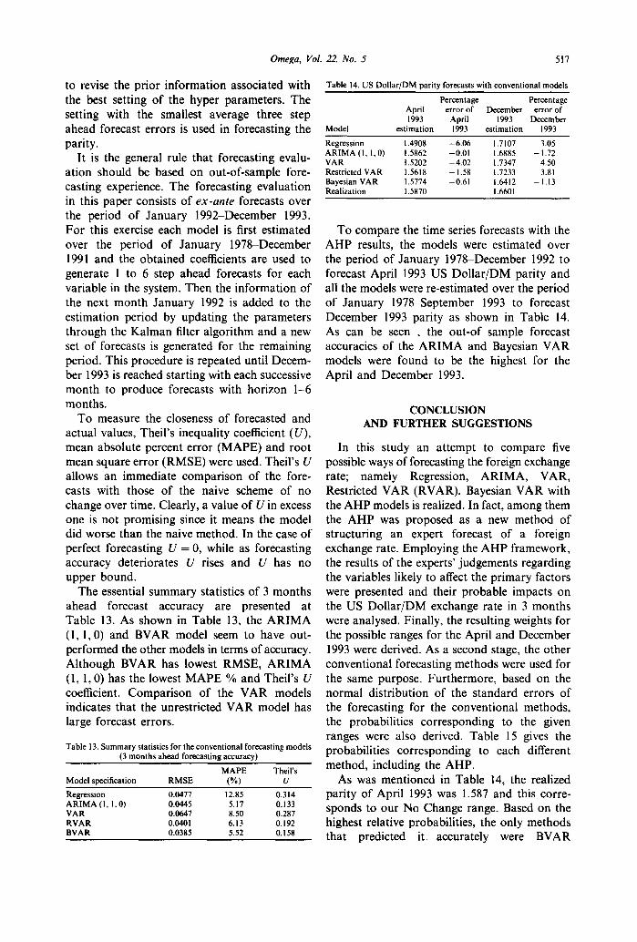
The essential summary statistics of 3 months ahead forecast accuracy are presented at Table 13. As shown in Table 13, the ARIMA (1, 1, 0) and BVAR model seem to have out- performed the other models in terms of accuracy. Although BVAR has lowest RMSE, ARIMA (1, 1, 0) has the lowest MAPE % and Theirs U coefficient. Comparison of the VAR models indicates that the unrestricted VAR model has large forecast errors.
Table 13. Summary statistics for the conventional forecasting models (3 months ahead forecasting accuracy)
MAPE Theirs Model specification RMSE (%) U
Regression 0.0477 12.85 0.314 ARIMA (I, I, 0) 0.0445 5.17 0.133 VAR 0.0647 8.50 0.287 RVAR 0.0401 6.13 0.192 BVAR 0.0385 5.52 0.158
Table 14. US Dollar/DM parity forecasts with conventional models
Model
Percentage Percentage April error of December error of 1993 April 1993 December
estimation 1993 estimation 1993
Regression 1.4908 - 6 . 0 6 1.7107 3.05 ARIMA (I, 1, 0) 1.5862 -0 .01 1.6885 - 1.72 VAR 1.5202 - 4 . 0 2 1.7347 4.50 Restricted VAR 1.5618 - 1.58 1.7233 3.81 Bayesian VAR 1.5774 -0 .61 1.6412 - 1.13 Realization 1.5870 1.6601
To compare the time series forecasts with the AHP results, the models were estimated over the period of January 1978-December 1992 to forecast April 1993 US Dollar/DM parity and all the models were re-estimated over the period of January 1978-September 1993 to forecast December 1993 parity as shown in Table 14. As can be seen , the out-of sample forecast accuracies of the ARIMA and Bayesian VAR models were found to be the highest for the April and December 1993.
CONCLUSION AND FURTHER SUGGESTIONS
In this study an attempt to compare five possible ways of forecasting the foreign exchange rate; namely Regression, ARIMA, VAR, Restricted VAR (RVAR), Bayesian VAR with the AHP models is realized. In fact, among them the AHP was proposed as a new method of structuring an expert forecast of a foreign exchange rate. Employing the AHP framework, the results of the experts' judgements regarding the variables likely to affect the primary factors were presented and their probable impacts on the US Dollar/DM exchange rate in 3 months were analysed. Finally, the resulting weights for the possible ranges for the April and December 1993 were derived. As a second stage, the other conventional forecasting methods were used for the same purpose. Furthermore, based on the normal distribution of the standard errors of the forecasting for the conventional methods, the probabilities corresponding to the given ranges were also derived. Table 15 gives the probabilities corresponding to each different method, including the AHP.
As was mentioned in Table 14, the realized parity of April 1993 was 1.587 and this corre- sponds to our No Change range. Based on the highest relative probabilities, the only methods that predicted it accurately were BVAR

518 Ulengin, Ulengin--Comparative Evaluation of AHP
Table 15. Probability distribution for Dollar/Mark parity (x), outcome ranges for April and December 1993
AHP Regression ARIMA VAR RVAR BVAR
April 1993 Sharp Decline x < 1.51 0.2067 0.7190 0.1635 0.3897 0.0764 0.0082 Moderate Decline 1.51 < x < 1.55 0.1608 0.2409 0.1593 0.4098 0.3095 0.0876 No Change 1.55 < x < 1.63 0.2425 0.0401 0.3912 0.1995 0.5913 0.6805 Moderate Increase 1.63 < x < 1.67 0.2275 0.0000 0.1441 0.0010 0.0220 0.197 I Sharp Increase x > 1.67 0.2025 0.0000 0.1401 0.0000 0.0008 0.0272
December 1993 Sharp Decline x < 1.56 0.1423 0.0000 0.0618 0.0000 0.0000 0.0073 Moderate Decline 1.56 < x < 1.61 0.2082 0.0025 0.1093 0.0037 0.0000 0.1741 No Change 1.61 < x < 1.70 0.2570 0.4418 0.4199 0.2574 0.2810 0.7815 Moderate Increase 1.70 < x < 1.75 0.3130 0.4426 0.2000 0.3906 0.5505 0.0154 Sharp Increase x > 1.75 0.0795 0.1131 0.2090 0.3483 0.1685 0.0000
(68.05%), RVAR (59.13%), ARIMA (39.12%) and the AHP (24.25%), among which BVAR and RVAR's predictions were relatively more accurate. On the other hand, the regression and VAR predictions (4.01 and 19.95% respectively, which both ranked the No Change range as a third possible range in terms of likelihood of occurrence, were really poor.
The actual parity of December 1993 was 1.66 and it is in the No Change zone. While the AHP (31.30%), VAR (39.06%) and RVAR (55.05%) approaches gave the highest probability to Moderate Increase, ARIMA (l, l, 0) (41.99%) and BVAR (78.15%) assigned the highest prob- ability to No Change. Regression model gave almost the same probability to No Change and Moderate Increase zones. In fact, BVAR was the only model that predicted the true region with the highest probability.
In reality, the AHP resulting weights were more uniformly distributed over the ranges then the conventional methods for April 1993. On December 1993 the probabilities given by the AHP tended to concentrate on specific zones but still not as clearly as the other methods. In fact, the same characteristics were also perceived in the AHP-based exchange rate prediction of Blair et al. [5] and of Saaty and Vargas [26]. The conventional methods assigned relatively low probabilities to the extreme ranges and this is due to the normal distribution assumption.
To our knowledge, this paper is the first one that investigates the predictive power of the AHP by comparing it with the other conventional forecasting methods. According to the results obtained, we can say that the AHP can be accepted as one of the three powerful methods in predicting the foreign exchange rate. How- ever, in order to generalize this conclusion, it is necessary to realise the same type of compar-
ative studies for different areas such as inflation rate and sales forecasts etc.
A P P E N D I X A
Formulation for the traditional econometr ic
approach
The general model was specified as
OR, = t 9 + ~ t j O R ~ _ j + ~ f l j U S A I , j y J
+ E 0jGERI, _j + ~ cSj USAR~_j J y
+ ~ ~pjGERR, _j + ~ zj USAPR,_j y J
+ ~ / z j G E R P R , _ j + ~ ~bj U S A M l t_j J J
+ ~ y j G E R M l, _j + ut J
and derived simple model
OR, = a 0 + a I O R t _ i + a2ORt - 2
+ a3 U S A R , + a 4 G E R R ,
+ a5 USAI , + a 6 G E R I ,
+ aTDR,_ l + u t
where
O R I = par i ty o f U S $ / D M at t ime t
U S A R , = interest rate o f U S A at t ime t
G E R R = interest rate o f G e r m a n y
U S A I = inflation rate o f U S A
G E R I = inflation rate o f G e r m a n y
D R = interest rate difference between U S A and G e r m a n y .

Omega, I/ol. 22, No. 5 519
In the f o r m u l a g iven a b o v e , a s are the
parameter s to be e s t i m a t e d and are expec ted to have the following signs:
a~ and a 2 are unrestricted,
a 3, a 6 > 0,
a 4, a 5 , a 7 < 0.
Explicit formulation for A R I M A (1, 1, O)
OR,(1 - B)(I - OB) = A,
where B is the back shift operator and A, is a sequence of independently distributed normal variables having mean zero and variance.
Formulation for the VAR model
For the variables X~, X2 . . . . . Xm the typical equation is
Xi, = f ( gt, - ,, XI,- 2 . . . . . g l , - L, 3(2,- I, X2,-2 . . . . .
X~,_L . . . . . Xo,,_,,Xm,_2 . . . . . xm,_,)
where L is some lag (L >/1).
A C K N O W L E D G E M E N T S
We are grateful to helpful comments made by the anonymous refeeres and the Editor on an earlier version of this paper.
R E F E R E N C E S
1. Akaike H (1973) Information theory and an extension of the maximum likelihood principle, In Second International Symposium on Information Theory (Edited by Petrov BN and Csaki F), pp. 267-281. Akademini Kiado, Budapest.
2. Alho JM (1992) Estimating the strength of expert judge- ment: the case of U.S. mortality forecast. J. Forecast. 11, 157-168.
3. Armstrong JS and Collopy F (1993) Causal forces: structuring knowledge for time-series extrapolation. J. Forecast. 12, 103-116.
4. Baghestani H and Mcnown R (1992) Forecasting the federal budget with time series models. J. Forecast. 11, 127--139.
5. Blair A, Nachtmann J, Olson J and Saaty TL (1987) Forecasting foreign exchange rates: an expert judgement approach. J. Socio-Econ. 21, 363-369.
6. Box GEP and Jenkins GM (1976) Time Series Analysis, Forecasting and Control. Holden Day, San Francisco, Calif.
7. Chishti SU, Hasan MA and Mahmud SF (1992) Macroeconometric modelling and Pakistan economy: a vector autoregressive approach. J. Dev. Ecom. 38, 353-370.
8. Doan T (1989) R A T S version 3.02 User's Manual. VAR Econometrics, Illinois.
9. Engle RF and Yoo BS (1987) Forecasting and testing in co-integrated systems. J. Economet. 35, 143-159.
10. Flides R (1991) Efficient use of information in the formation of subjective industry forecast. J. Forecast. 10, 597-618.
I I. Fuller WA (1976) Introduction to Statistical Time Series. Wiley, New York.
12. Funke M (1990) Assessing the forecast accuracy of monthly vector autoregressive models: the case of five OECD countries. Int. J. Forecast. 6, 363-378.
13. Funke M (1992) Time series forecasting of the German unemployment rate. J. Forecast. 11, 111-125.
14. Geweke J and Meese R (1981) Estimating regression models of finite but unknown order. Int. Economet. Retd. 22, 55-70.
15. Hannah EJ and Quin BG (1979) The determination of the order of an autoregression. J. R. Statist Soc. Ser. B 41, 190-195.
16. Holden K and Broomhead A (1990) An examination of vector autoregressive forecasts for the U.K. economy. Int. J. Forecast. 6, 11-23.
17. Kaylen MS (1988) Vector autoregression forecasting models: recent developments applied to the U.S. hog market. Am. J. Agric. Econ. 70, 701-712.
18. King S (1983) Real interest rates and the interaction of money, output and prices. Mimeo. Northwestern University. Evanston, I11.
19. Klayman J and Schoemaker PJH (1993) Thinking about the future: a cognitive perspective. J. Forecast. 12, 161-178.
20. Kling JL and Bessler DA (1984) A comparison of multivariate forecasting procedures for economic time series. Paper presented at the Fourth International Symposium on Forecasting, London, England.
21. Literman RB (1986) Forecasting with Bayesian Vector Autoregressious--five years of experience. J. Bus. Econ. Statist. 4, 25-38.
22. Lupoletti W and Webb RH (1986) Defining and improving the accuracy of macroeconomic forecasts: Contributions from a VAR model. J. Bus. 59, 263- 285.
23. Nerlove M, Grether DM and Carvalho JL (1979) Analysis o f Economic Time Series: A synthesis. Academic Press, New York.
24. Runkle D (1987) Vector autoregressions and reality. J. Bus. Econ. Statist. 5, 437 442.
25. Saaty TL (1988) Multicriteria Decision Making: The Analytical Hierarchy Process. RWS, Pittsburgh.
26. Saaty TL and Vargas LG (1991) Prediction, Pro/ection and Forecasting. Kluwer Academic, Boston.
27. Sims C (1980) Macroeconomics and reality. Econometrica 48, 1 48.
28. Sims C (1987) Comment. J. Bus. Econom. Statist. 5, 443-449.
29. Sims C (1989) Models and their uses. Am. J. Agric. Econ. 71, 489-494.
30. Spencer D (1989) Does money matter? The robustness of evidence from vector autoregression. J. Monet. Econ. 5, 171 186.
31. Tiao GC and Box GEP (1981) Modelling multiple time series with applications. J. Am. Statist. Ass. 75, 802-816.
32. Tiao GC and Tsay RS (1983) Multiple time series modelling and extended sample cross-correlations. J. Bus. Econ. Statist. 1, 43 56.
33. Todd R (1990) Vector autoregression evidence on monetarism: another look at the robustness debate. Fed. Bank Mineap. Q. Rev. Spring, 19-37.
34. Woo W (1985) The monetary approach to exchange rate determination under rational expectations. J. Int. Econ. 18, 1-16.
ADDRESS FOR CORRESPONDENCE: Dr Fiisun ~lengin, Istanbul Teknik Universitesi, lsletme Fakiiltesi, Endiistri Miih. B61., 80680 Ma£ka, Istanbul, Turkey.