forecasting economic growth for estonia: application of common
TRANSCRIPT
Working Paper Series
9/2007
Eesti Pank Bank of Estonia
Forecasting Economic Growth for Estonia:Application of Common FactorMethodologies
Christian Schulz

Forecasting Economic Growth for Estonia:Application of Common Factor
Methodologies
Christian Schulz
Abstract
In this paper, the application of two different unobserved factor mod-els to a data set from Estonia is presented. The small-scale state-spacemodel used by Stock and Watson (1991) and the large-scale static prin-cipal components model used by Stock and Watson (2002) are employedto derive common factors. Subsequently, using these common factors,forecasts of real economic growth for Estonia are performed and evalu-ated against benchmark models for different estimation and forecastingperiods. Results show that both methods show improvements over thebenchmark model, but not for the all the forecasting periods.
JEL Code: C53, C22, C32, F43
Keywords: Estonia, forecasting, principal components, state-space model,forecast performance
Author’s e-mail address: [email protected]
The views expressed are those of the author and do not necessarily representthe official views of Eesti Pank.
Non-technical summary
The forecasting of economic growth draws a lot of attention in all countriesand new methods are constantly being developed to improve the performanceof forecasting models. While all of these methods are universally applicablein principle, their appropriateness for particular settings has to be examined.As more and more macroeconomic time series data becomes easily available,there has been a shift in the development of these methods towards the inclu-sion of more time series into the forecasting models. One promising field isthe study of unobservable common factors in large data sets, where the as-sumption is made that a small number of factors drive the whole data set andthat the use of these factors can improve forecasts.
In this paper we apply two different methods to extract common factorsfrom an Estonian data set of quarterly macroeconomic time series from 1994to 2006. One is a small-scale state-space model which has been used by Stockand Watson (1991) for economic forecasting. This model is estimated usingmaximum likelihood and a Kalman filter procedure. As the number of timeseries variables, which can be included in this model, is small, it requirescareful pre-selection. We use different specifications of the model, each basedon three time series. To represent specificities of the Estonian economy, weinclude survey type data such as industrial order books as well as financialdata such as monetary supply and stock exchange data. The latter two reflectthe fact that our analysis suggests that financial data are more relevant forforecasts of the Estonian economy than other authors have found for manymature economies.
The second methodology we apply draws on the principal components lit-erature. Following Stock and Watson (2002), we use a static principal compo-nents model based on a large data set of 34 time series, which represent a largepart of the total available data set. This method is computationally rather sim-ple and is computed for a contemporaneous data set and a “stacked” data set.The latter includes the first lags of the 34 time series to allow for the existenceof phase shifts. This analysis yields several factors which can be interpretedwith respect to the influence individual time series have upon them.
We follow a large part of the literature on forecasting in concluding with theevaluation of our resulting forecasting models compared to a benchmark naïvemodel. In-sample comparisons and out-of sample comparisons are presented.The latter uses a sub-sample of the whole data set to estimate the forecastingequation and then uses the remainder of the sample to evaluate and comparethe performance.
The in-sample forecast evaluation according to Diebold and Mariano (1995)shows that our models outperform the naïve forecast for most of the evalua-
2

tion periods, particularly for the period of the Russian crisis in the late 1990s.However, this outperformance is not always significant and particularly forthe end of the sample most models are actually worse than the naïve forecast.The out-of sample tests according to Clark and McCracken (2001) show thatthe additional information included in our models is not statistically irrelevant,however. The naïve model does not encompass our forecasting models.
Overall, common factor models do improve forecasts and reveal a lot ofinformation about the underlying data set, particularly for the principal com-ponents approach.
3

Contents
1. Introduction . . . . . . . . . . . . . . . . . . . . . . . . . . . . . . 5
2. Specific features of the Estonian economy. . . . . . . . . . . . . . 6
3. Identification of leading time series. . . . . . . . . . . . . . . . . . 13
4. Common factor methodologies. . . . . . . . . . . . . . . . . . . . 174.1. The state-space model. . . . . . . . . . . . . . . . . . . . . . 174.2. Static principal components. . . . . . . . . . . . . . . . . . . 24
5. Forecast comparison. . . . . . . . . . . . . . . . . . . . . . . . . 33
6. Conclusions. . . . . . . . . . . . . . . . . . . . . . . . . . . . . . 37
References. . . . . . . . . . . . . . . . . . . . . . . . . . . . . . . . . 39
Appendix 1. Data set and cross correlations. . . . . . . . . . . . . . . 42
Appendix 2. Principal components: time series included. . . . . . . . 45
4

1. Introduction
The Estonian economy has been growing quickly since the country re-gained its independence in the early nineties and this growth has recently in-creased to double digits, vastly exceeding the potential of 5–7% defined bythe Bank of Estonia. Being able to make accurate predictions about such highgrowth rates is extremely relevant for policy makers and is pursued by sev-eral institutions both in Estonia and internationally. This paper extends themethodology currently used by the Bank of Estonia for short-term forecastingto include the use of common factor methodologies; namely, state-space dy-namic common factor models and principal components analysis. We focusresearch on the prediction of economic growth, but similar models can also beused to forecast inflation or other macroeconomic variables.
State-space modelling was introduced to economic forecasting by Stockand Watson (1991). The idea is that from a small set of potentially leadingvariables a common dynamic trend is extracted, which excludes much of theidiosyncratic movements of the individual series. State-space modelling isused to describe the dynamic framework, the coefficients of which are sub-sequently estimated using Kalman filtering techniques. The result is a singleleading indicator that can then be tested for its predictive capacity. Principalcomponents analysis comes in two different forms — static and dynamic. Sta-tic principal components are widely used and have, for instance, been used byStock and Watson (2002) for economic forecasting. It is an efficient methodfor deriving common factors from a large set of data. The idea is to derive com-ponents that explain the largest part of the cross-sectional variance. Therefore,static principal components are based on the variance-covariance matrix of adata set and can easily be computed using any standard econometric softwarepackage. Dynamic principal component methodology for economic forecast-ing was developed by Forni et al. (2000). It is based on the spectral densitymatrix of a data set and requires more specific software. We leave this applica-tion to future research. Obviously, evaluating the performance of the derivedleading indicators requires some attention as well. We will use in-sample andout-of-sample tests to evaluate the performance of these indicators.
The remainder of this paper is laid out as follows. Section 2 takes a closerlook at some of the specific features of the Estonian economy which need to betaken into account when constructing forecasts. In Section 3, we take a lookat the data set and preliminarily analyse its predictive powers. In Section 4,we use dynamic common factor analysis following Stock and Watson (1991)to construct a leading indicator and evaluate its performance. In Section 5,the static principal components model is presented and a leading indicator isderived. This is then evaluated and compared to other forecasting models. Our
5
conclusion is presented in Section 6.
2. Specific features of the Estonian economy
In this section we will focus on two aspects of the Estonian economy thatmay be important when trying to forecast future economic growth. One as-pect is the existence of cycles, specifically growth cycles that may help whenmaking forecasts. The other aspect is how the Estonian economy differs fromother economies.
If we want to predict the economic situation in Estonia, we first have tolook at its growth pattern over the period we can consider. To avoid the earlytransition pains encountered by Estonia as it struggled to shake off Soviet in-fluence, we start in the first quarter of 1995. Another reason for beginningthere is that the data before this period is only partially available and of some-times questionable quality. At this time, we use the GDP time series as theywere published before 2006. In 2006, major changes were made in the collec-tion and calculation methodologies as part of the harmonisation process withEU standards. This update changed GDP levels by up to 6.0%, according tothe Annual Report 2006 of Statistics Estonia, and growth figures, which aremore relevant to this paper, changed somewhat as well. Unfortunately, onlydata from 2000 onwards is currently available under the new methodology.This time span is too short for the methodologies we employ later on. There-fore, we must link the old and new data before the longer time series under thenew methodology is set and published by the Statistics Office of Estonia laterthis year.
In the Figure 1 year-on-year-growth (from –4% up to +16%) is presentedon the y-axis. It can be seen that since 2000, growth has fluctuated but hasbeen positive throughout. Before, there was a brief phase of strong growthrunning up until 1998, followed by a sharp decline in growth and even a briefperiod of negative growth. It can also be seen that growth has significantlyexceeded the long-term corridor between 5% and 9% since 2005.
In addition to economic growth as such, the reliable signalling of economicphases or business cycles is often required from forecasts and specifically fromleading indicators. In business cycle analysis, the output gap is commonlyused to identify the current position in the cycle. It represents the current usageof the production capacity of an economy. Under-usage of capacity indicatesa recession; over-usage indicates a boom, with up- and downswings in be-tween. The Ifo Institute for Economic Research has found an intuitive graphic
6

-.04
.00
.04
.08
.12
.16
1996 1998 2000 2002 2004 2006
GDP_EST_YOYGR_LINKED
Figure 1: Real GDP Growth in Estonia (% yoy, constant 2000 prices)
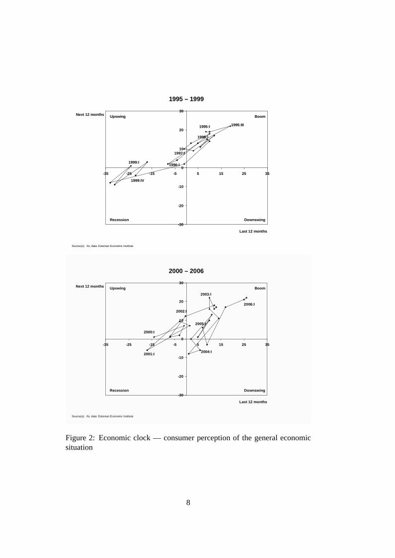
way of illustrating the current position of an economy (CESIfo, 2007)1. The“economic climate clock” plots an indicator of the perception of the current(or very recent) climate of the economy versus expectations. We do this forEstonia using the consumer climate indices published by the Estonian Eco-nomic Institute for the past twelve months (recent climate) and the comingtwelve months (expectations). As the Russian crisis of 1998 clearly marks abreak, we display two different graphs below: one for the period 1995–1999,the other for 2000–2006 (see Figure 2).
The four quadrants of the “economic clock” have different interpretationsaccording to the relationship between the expectations and interpretations ofthe current situation or recent past. Table 1 represents interpretations for thedifferent quadrants.
Neither of the two periods exhibits the typical smooth development fromone economic phase to another2. Instead, there seems to be a lot more vari-ation than we would find in more mature economies. From 1997 to 1998,the Russian crisis seemed to have taken the Estonian consumers by surprise,which is why the clock turned from boom to bust within a period of only twoquarters. The second quadrant “downturn” was skipped; the economy dropped
1For further details on the economic clock and examples for Germany, see Nerb (2007).2For examples of mature economies, see Nerb (2007).
7
Source(s): ifo, data: Estonian Economic Institute
-30
-20
-10
0
10
20
30
-35 -25 -15 -5 5 15 25 35
Next 12 months
Last 12 months
1995 – 1999
Boom
DownswingRecession
Upswing
1999:IV
1995:III1995:I
1996:I
1997:I
1998:I
1999:I
Source(s): ifo, data: Estonian Economic Institute
-30
-20
-10
0
10
20
30
-35 -25 -15 -5 5 15 25 35
Next 12 months
Last 12 months
2000 – 2006
Boom
DownswingRecession
Upswing
2000:I
2006:I
2005:I
2004:I
2003:I
2002:I
2001:I
Figure 2: Economic clock — consumer perception of the general economicsituation
8
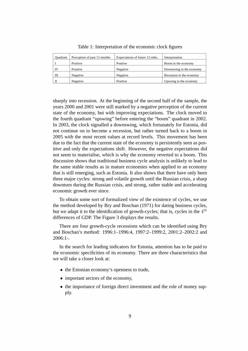
Table 1: Interpretation of the economic clock figures
Quadrant Perception of past 12 months Expectations of future 12 mths. Interpretation
I Positive Positive Boom in the economy
IV Positive Negative Downswing in the economy
III Negative Negative Recession in the economy
II Negative Positive Upswing in the economy
sharply into recession. At the beginning of the second half of the sample, theyears 2000 and 2001 were still marked by a negative perception of the currentstate of the economy, but with improving expectations. The clock moved tothe fourth quadrant “upswing” before entering the “boom” quadrant in 2002.In 2003, the clock signalled a downswing, which fortunately for Estonia, didnot continue on to become a recession, but rather turned back to a boom in2005 with the most recent values at record levels. This movement has beendue to the fact that the current state of the economy is persistently seen as pos-itive and only the expectations shift. However, the negative expectations didnot seem to materialise, which is why the economy reverted to a boom. Thisdiscussion shows that traditional business cycle analysis is unlikely to lead tothe same stable results as in mature economies when applied to an economythat is still emerging, such as Estonia. It also shows that there have only beenthree major cycles: strong and volatile growth until the Russian crisis, a sharpdownturn during the Russian crisis, and strong, rather stable and acceleratingeconomic growth ever since.
To obtain some sort of formalized view of the existence of cycles, we usethe method developed by Bry and Boschan (1971) for dating business cycles,but we adapt it to the identification of growth-cycles; that is, cycles in the4th
differences of GDP. The Figure 3 displays the results.
There are four growth-cycle recessions which can be identified using Bryand Boschan’s method: 1996:1–1996:4, 1997:2–1999:2, 2001:2–2002:2 and2006:1-.
In the search for leading indicators for Estonia, attention has to be paid tothe economic specificities of its economy. There are three characteristics thatwe will take a closer look at:
• the Estonian economy’s openness to trade,
• important sectors of the economy,
• the importance of foreign direct investment and the role of money sup-ply.
9

-.04
.00
.04
.08
.12
.16
1996 1998 2000 2002 2004 2006
GDP_EST_YOYGR_LINKED
Figure 3: Growth cycle recessions in Estonia
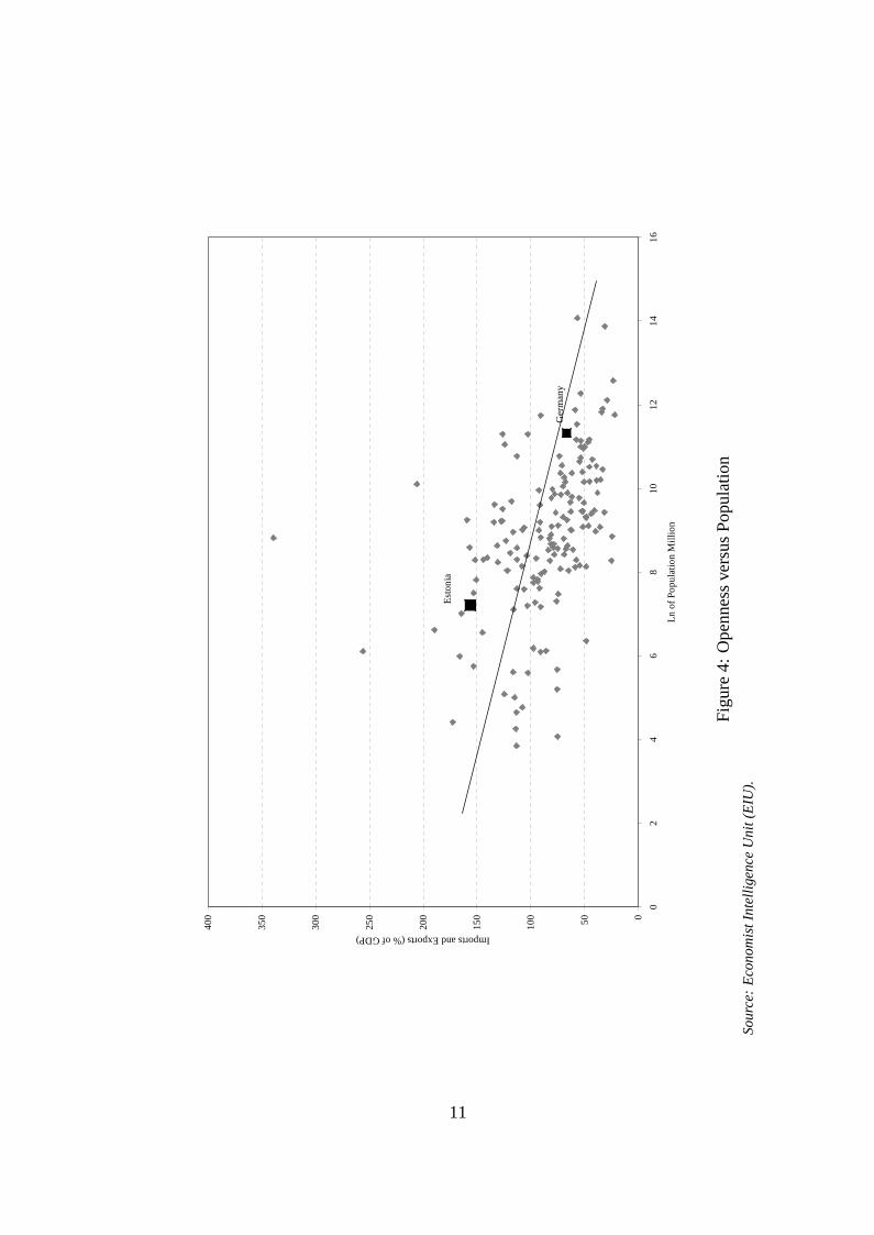
Estonia is one of the world’s most open economies, with trade (the sum ofimports and exports of goods and services) amounting to almost 160% of thegross domestic product (see Figure 4). Therefore, when predicting macroeco-nomic variables for Estonia, special consideration might be taken of variablesthat represent the influence of trade on the Estonian economy. It should benoted, however, that openness seems to be a function of the size of an econ-omy. This is shown in the following figure, which demonstrates that there isa negative linear relationship between the size of a country, represented by itspopulation in Log-terms, and its openness.
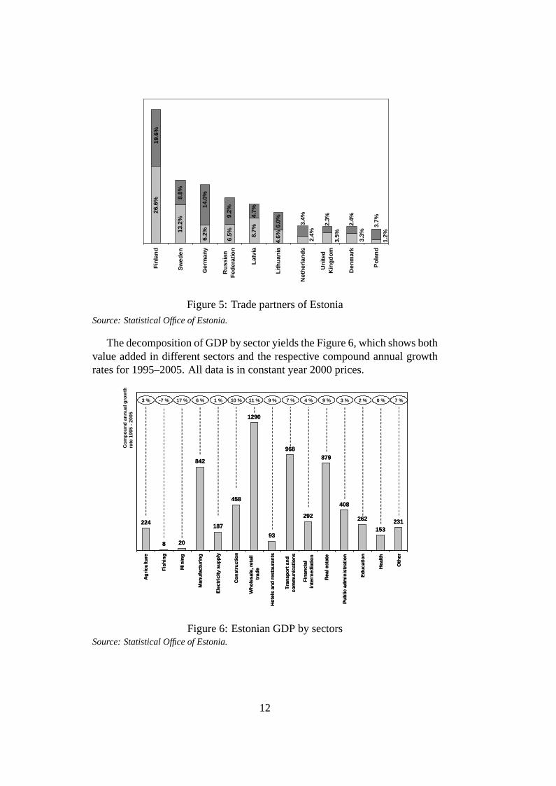
Estonia is a very open economy, but it is not an outlier given the relation-ship above. This is reflected in the fact that we find Estonia above the esti-mated OLS-regression line, but not dramatically so3. Nonetheless, because ofthe importance of trade, we include macroeconomic variables from Estonia’simportant trade partners in the data set. We selected variables from Finland,the Euro zone and Russia, as these countries and areas comprise Estonia’smost important trade partners, as can be seen in the Figure 5.
3The negative-sloping regression line shows that generally, in smaller countries, tradeplays a bigger role than in larger ones.
10
050100
150
200
250
300
350
400
02
46
810
1214
16
Ln
of P
opul
atio
n M
illio
n
Imports and Exports (% of GDP)
Est
onia
Ger
man
y
Fig
ure
4:O
penn
ess
vers
usP
opul
atio
nS
ou
rce
:E
con
om
istI
nte
llige
nce
Un
it(E
IU).
11
26.6
%
13.2
%
6.2% 8.
7%
4.6%
8.8%
4.7%
6.0%
2.4%
3.5%
3.3%
1.2%6.5%
3.7%2.4%
2.3%
3.4%
19.6
%
9.2%
14.0
%
Fin
lan
d
Sw
eden
Ger
man
y
Ru
ssia
nF
eder
atio
n
Lat
via
Lith
uan
ia
Net
her
lan
ds
Un
ited
Kin
gd
om
Den
mar
k
Po
lan
d
Figure 5: Trade partners of EstoniaSource: Statistical Office of Estonia.
The decomposition of GDP by sector yields the Figure 6, which shows bothvalue added in different sectors and the respective compound annual growthrates for 1995–2005. All data is in constant year 2000 prices.
3 % -7 % 17 % 6 % 1 % 10 % 11 % 9 % 7 % 4 % 9 % 3 % 2 % 0 % 7 %
Co
mp
ou
nd
an
nu
al g
row
th
rate
199
5 -
2005
224
8 20
842
187
458
1290
93
968
292
879
408
262
153231
Ag
ricu
ltu
re
Fis
hin
g
Min
ing
Man
ufa
ctu
rin
g
Ele
ctri
city
su
pp
ly
Co
nst
ruct
ion
Wh
ole
sale
, ret
ail
trad
e
Ho
tels
an
d r
esta
ura
nts
Tra
nsp
ort
an
dco
mm
un
icat
ion
s
Fin
anci
alin
term
edia
tio
n
Rea
l est
ate
Pu
blic
ad
min
istr
atio
n
Ed
uca
tio
n
Hea
lth
Oth
er
Figure 6: Estonian GDP by sectorsSource: Statistical Office of Estonia.
12

The largest sectors are trade (retail and wholesale), transport, real estateand manufacturing. Growth is spread rather evenly across sectors, with thesecondary sector somewhat underperforming the tertiary sector. These resultsdo not reveal ex-ante suppositions about possible leading indicators; however,the eventual choice of variables should be checked against this composition toavoid the use of economically insignificant variables. This would be the casefor instance, if fishing turned out to be a good leading indicator statistically(which indeed it does).
Foreign direct investment is important to the Estonian economy for tworeasons. First, it can be seen as a proxy for overall investment. Second, itis, as Zanghieri (2006) points out, the “only non-debt-creating foreign sourceof capital” to finance Estonia’s persistent current account deficit (Zanghieri,2006:257). There is a considerable amount of literature on the qualities offinancial variables as leading indicators for economic cycles; for instance, Es-trella and Mishkin (1998) and Fritsche and Stephan (2000). In general, theirfindings state that there are only very limited and unstable empirical relation-ships in developed countries. Yet for Estonia, the particularities of its economywill lead to different results, as this paper will suggest. This may be due toEstonia’s monetary regime, the currency board linked with the Deutschmark(since 1999 with all European currencies and subsequently, the euro).
3. Identification of leading time series
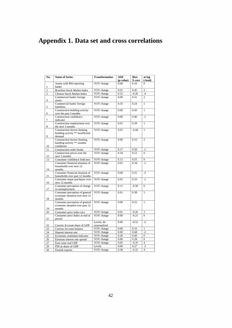
There is a table in the appendix containing all the time series available insufficient length and frequency as well as their respective cross-correlationcharacteristics with respect to real GDP growth as a reference series4. Thetable indicates the transformations made to achieve stationarity, their respec-tive unit-root-test results (augmented Dickey-Fuller test) and maximum cross-correlations, and the lag (positive number) or lead (negative number) at whichthis maximum cross-correlation is recorded.
In the following section, we will explore the leading or lagging character-istics of the different types of variables with respect to real GDP growth inEstonia. The data was categorised into four groups: (1) financial variables, (2)trade variables, (3) GDP-sector variables and (4) survey-type variables.
The financial variables included in the data set exhibit very different char-
4Using cross-correlations to analyse the lagging and leading characteristics of variableswith respect to each other is standard in the empirical literature — for instance, see Bandholzand Funke (2003), and Forni et al. (2001). Gerlach and Yiu (2005) use contemporaneouscorrelations and principal components to pre-identify variables useful for the construction ofa common factor of economic activity in Hong Kong.
13
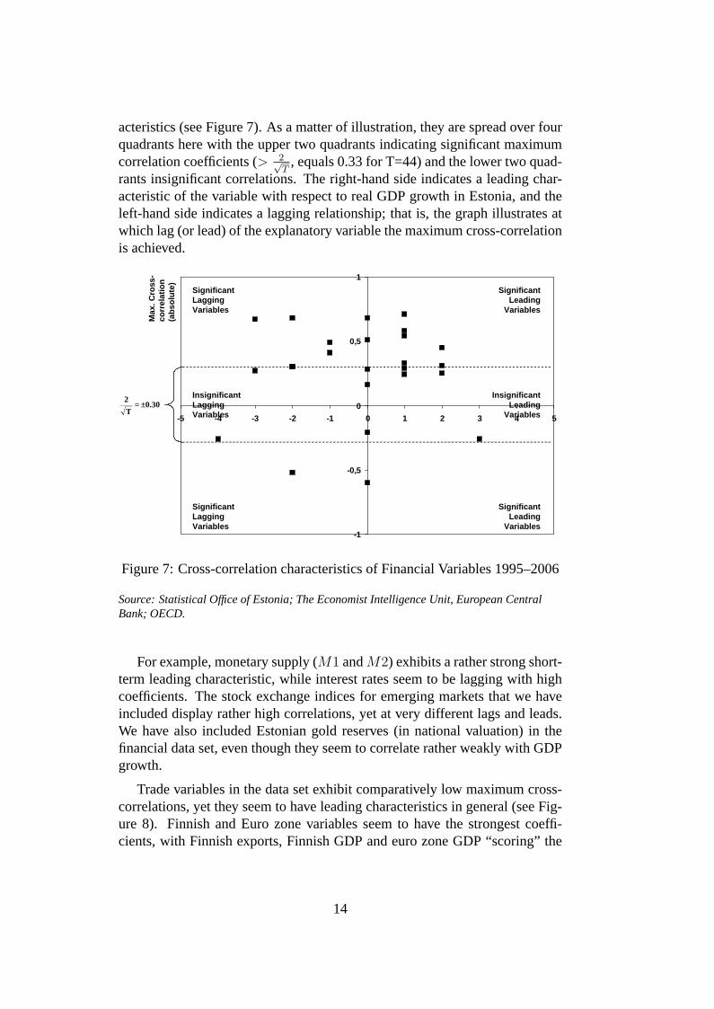
acteristics (see Figure 7). As a matter of illustration, they are spread over fourquadrants here with the upper two quadrants indicating significant maximumcorrelation coefficients (> 2√
T, equals 0.33 for T=44) and the lower two quad-
rants insignificant correlations. The right-hand side indicates a leading char-acteristic of the variable with respect to real GDP growth in Estonia, and theleft-hand side indicates a lagging relationship; that is, the graph illustrates atwhich lag (or lead) of the explanatory variable the maximum cross-correlationis achieved.
-1
-0,5
0
0,5
1
-5 -4 -3 -2 -1 0 1 2 3 4 5
Max
. Cro
ss-
corr
elat
ion
(a
bso
lute
)
Significant Lagging Variables
Significant Leading
Variables
Insignificant Lagging Variables
Insignificant Leading
Variables0.30
T
2 ±=
Significant Lagging Variables
Significant Leading
Variables
Figure 7: Cross-correlation characteristics of Financial Variables 1995–2006
Source: Statistical Office of Estonia; The Economist Intelligence Unit, European CentralBank; OECD.
For example, monetary supply (M1 andM2) exhibits a rather strong short-term leading characteristic, while interest rates seem to be lagging with highcoefficients. The stock exchange indices for emerging markets that we haveincluded display rather high correlations, yet at very different lags and leads.We have also included Estonian gold reserves (in national valuation) in thefinancial data set, even though they seem to correlate rather weakly with GDPgrowth.
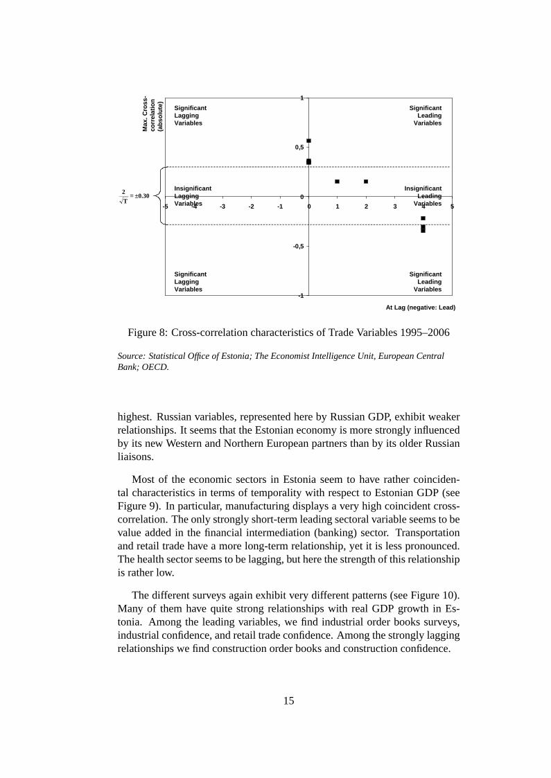
Trade variables in the data set exhibit comparatively low maximum cross-correlations, yet they seem to have leading characteristics in general (see Fig-ure 8). Finnish and Euro zone variables seem to have the strongest coeffi-cients, with Finnish exports, Finnish GDP and euro zone GDP “scoring” the
14
-1
-0,5
0
0,5
1
-5 -4 -3 -2 -1 0 1 2 3 4 5
At Lag (negative: Lead)
Max
. Cro
ss-
corr
elat
ion
(a
bso
lute
)
Significant Lagging Variables
Significant Leading
Variables
Insignificant Lagging Variables
Insignificant Leading
Variables0.30
T
2 ±=
Significant Lagging Variables
Significant Leading
Variables
Figure 8: Cross-correlation characteristics of Trade Variables 1995–2006
Source: Statistical Office of Estonia; The Economist Intelligence Unit, European CentralBank; OECD.
highest. Russian variables, represented here by Russian GDP, exhibit weakerrelationships. It seems that the Estonian economy is more strongly influencedby its new Western and Northern European partners than by its older Russianliaisons.
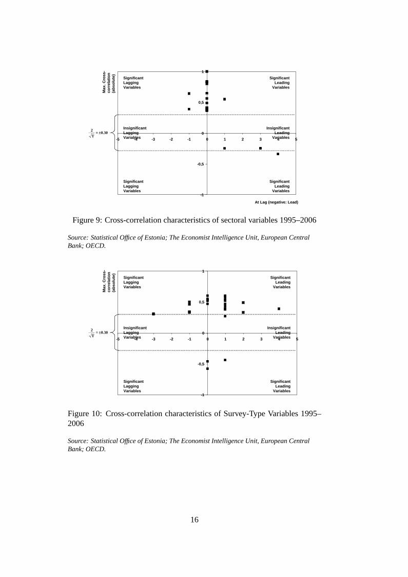
Most of the economic sectors in Estonia seem to have rather coinciden-tal characteristics in terms of temporality with respect to Estonian GDP (seeFigure 9). In particular, manufacturing displays a very high coincident cross-correlation. The only strongly short-term leading sectoral variable seems to bevalue added in the financial intermediation (banking) sector. Transportationand retail trade have a more long-term relationship, yet it is less pronounced.The health sector seems to be lagging, but here the strength of this relationshipis rather low.
The different surveys again exhibit very different patterns (see Figure 10).Many of them have quite strong relationships with real GDP growth in Es-tonia. Among the leading variables, we find industrial order books surveys,industrial confidence, and retail trade confidence. Among the strongly laggingrelationships we find construction order books and construction confidence.
15
-1
-0,5
0
0,5
1
-5 -4 -3 -2 -1 0 1 2 3 4 5
At Lag (negative: Lead)
Max
. Cro
ss-
corr
elat
ion
(a
bso
lute
)
Significant Lagging Variables
Significant Leading
Variables
Insignificant Lagging Variables
Insignificant Leading
Variables0.30
T
2 ±=
Significant Lagging Variables
Significant Leading
Variables
Figure 9: Cross-correlation characteristics of sectoral variables 1995–2006
Source: Statistical Office of Estonia; The Economist Intelligence Unit, European CentralBank; OECD.
-1
-0,5
0
0,5
1
-5 -4 -3 -2 -1 0 1 2 3 4 5
Max
. Cro
ss-
corr
elat
ion
(a
bso
lute
)
Significant Lagging Variables
Significant Leading
Variables
Insignificant Lagging Variables
Insignificant Leading
Variables0.30
T
2 ±=
Significant Lagging Variables
Significant Leading
Variables
Figure 10: Cross-correlation characteristics of Survey-Type Variables 1995–2006
Source: Statistical Office of Estonia; The Economist Intelligence Unit, European CentralBank; OECD.
16

4. Common factor methodologies
4.1. The state-space model
In this section, we will employ methods originally developed by Kalman(1960) and Kalman (1963) to estimate a dynamic common factor model andto construct a leading indicator for the Estonian economy. This approach wasinitially also favoured by Stock and Watson (1991). The same methodologyhas been used successfully by other authors, for instance, Bandholz and Funke(2003) for Germany, Gerlach and Yiu (2005) for Hong Kong, and Curran andFunke (2006) for China.
The dynamic factor model’s main identifying assumption is that the co-movements of the indicator series (observed variables) arise from one singleunobserved common factor. This factor is expected to provide better forecastsof the reference series than the individual indicator series. The factor is con-structed only from the observed series; that is, the reference series — in ourcase real GDP growth — is not used in the process. Constructing the com-mon factor involves (1) formulating the model, (2) converting the model tostate-space representation and (3) estimating the parameters using maximumlikelihood (MLE) methodology, for which the Kalman filter is employed. TheKalman filter is composed of two recursive stages: (1) filtering and (2) smooth-ing. Filtering involves estimating the common factor for periodt on the basisof information available at periodt − 1. The forecast error is minimised us-ing MLE. The second stage, smoothing, then takes account of the informa-tion available over the entire sample period. The algorithm is computationallyrather expensive; that is, achieving the convergence of the different coefficientsand parameters is time-consuming5. Because of this technical restriction, onlya few variables can be included in the model. This requires a careful selec-tion of the input variables, for which there are numerous criteria. These arewell summarised by Bandholz (2004). Among the formal criteria we find thefollowing:
• A significant relationship between the lagged leading variable and thereference series in terms of general fit.
• The stability of this relationship.
• Improved out-of-sample forecasting.
• Timely identification of all turning points to avoid incorrect signals.
5The software we employed was kindly made available by Chang-Jin Kim and is de-scribed in Kim (1999).
17
Moreover, there are a number of informal criteria which should be lookedat:
• Timely publication.
• High publication frequency
• Not subject to major ex-post revisions.
• Existence of theoretical background for leading relationship.
First, we would like to focus on the discussion of which system of lead-ing variables might well represent the Estonian economy. For the Germaneconomy, industrial indicators such as order books are used as manufacturingplays a significant role there (Bandholz and Funke, 2003). For China, indi-cators representing the stock market, the real estate market and the exportsindustry are used as it is believed that these sectors play significant roles (Cur-ran and Funke, 2006). Gerlach and Yiu (2005) use four different series forHong Kong: namely, a stock market index, a residential property index, retailsales and total exports.
The mechanical choice of those variables that show their most significantcross-correlation with the reference series at lag 1 might be the obvious wayforward, but we deviate here. Value added in financial services could be thethird variable, but it would be rather problematic. There is no obvious eco-nomic reason why the banking and insurance sectors should lead economicgrowth. In fact, a lagging characteristic would be expected. Therefore, in or-der to avoid correlation by plain statistical coincidence, we will abstain fromusing this variable. We use real growth inM1 to represent monetary con-ditions and industrial order books to reflect business conditions. As a thirdvariable, real growth in loans to individuals might be used to reflect the im-portance of private consumption, though a criticism can be levelled thatM1and loans to individuals might be correlated not just statistically (which theyare), but also theoretically, as M1 drives credit growth via minimum reserverequirements. Therefore, we use a stock exchange index to reflect asset mar-kets as an alternative. However, this comes at the cost of reducing the samplesize, as stock market data is only available from 1996 onwards; that is, year-on-year growth rates are only available from 1997 onwards6. Therefore, wewill display the results for both estimations and vary the variableY 3 accordingto the two alternatives in the following. Table 2 displays the criteria by whichthe variables were chosen.
In the following, we derive the state-space model following the notation byKim (1999). LetYt be the vector of the time series from which the common
6In fact, stock indices for Tallinn are available on the website www.ee.omxgroup.comonly from 2000 onwards. We have prolonged the series using old Riga stock exchange data.
18

Table 2: List of leading indicators
Selected Variables
Industrial Orderbooks (Survey)
Formal Criteria
Max. Cross-correlation 0.61
At lag 1
Informal Criteria
Good indicator for important industrial sector
Real Money Supply M1 (year-on-year growth rate)
Max. Cross-correlation 0.74
At lag 1
Currency Board ER system means direct influence from payments balance
Real Loans to Individuals (year-on-year growth rate)
Max. Cross-correlation 0.59
At lag 1
Drives Consumption
Tallinn Stock Exchange Index(year-on-year growth rates from1997 onwards)
Max. Cross-correlation 0.54
At lag 1
Incorporates Expectations
factor will be derived. Its four elements are fourth differences in quarterlyoverall industrial order books(Y1t), the year-on-year real growth of monetarysupplyM1 (Y2t) and year-on-year real growth in loans to individuals or theTallinn Stock Exchange Index, respectively(Y3t). The unobserved commoncomponent is denoted byIt.
Y1t = D1 + γ10It + e1t (1)
Y2t = D2 + γ20It + e2t (2)
Y3t = D3 + γ30It + e3t (3)
(It − δ) = φ(It−1 − δ) + ωt, $ ∼ iidN (0, 1) (4)
eit = Ψi,1ei,t−1 + εit, εit ∼ iidN(0, σ2
i
)and i = 1, 2, 3 (5)
As constantsDi andδ cannot be separately identified, we write the modelin terms of deviations from means. This concentrated form of the model isrepresented as follows:
y1t = γ10it + e1t (6)
y2t = γ20it + e2t (7)
y3t = γ30it + e3t (8)
it = φit−1 + ωt, $ ∼ iidN (0, 1) (9)
eit = Ψi,1ei,t−1 + εit, εit ∼ iidN(0, σ2
i
)and i = 1, 2, 3 (10)
19
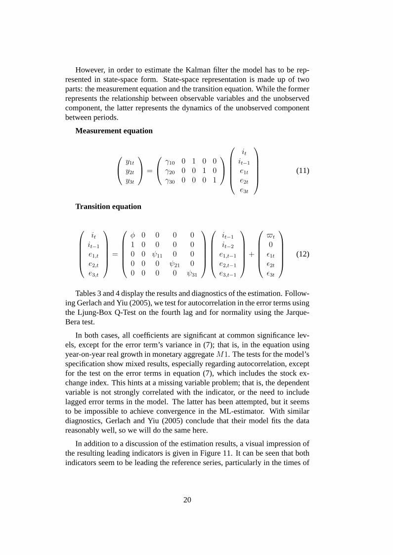
However, in order to estimate the Kalman filter the model has to be rep-resented in state-space form. State-space representation is made up of twoparts: the measurement equation and the transition equation. While the formerrepresents the relationship between observable variables and the unobservedcomponent, the latter represents the dynamics of the unobserved componentbetween periods.
Measurement equation
y1t
y2t
y3t
=
γ10 0 1 0 0γ20 0 0 1 0γ30 0 0 0 1
itit−1
e1t
e2t
e3t
(11)
Transition equation
itit−1
e1,t
e2,t
e3,t
=
φ 0 0 0 01 0 0 0 00 0 ψ11 0 00 0 0 ψ21 00 0 0 0 ψ31
it−1
it−2
e1,t−1
e2,t−1
e3,t−1
+
$t
0ε1t
ε2t
ε3t
(12)
Tables 3 and 4 display the results and diagnostics of the estimation. Follow-ing Gerlach and Yiu (2005), we test for autocorrelation in the error terms usingthe Ljung-Box Q-Test on the fourth lag and for normality using the Jarque-Bera test.
In both cases, all coefficients are significant at common significance lev-els, except for the error term’s variance in (7); that is, in the equation usingyear-on-year real growth in monetary aggregateM1. The tests for the model’sspecification show mixed results, especially regarding autocorrelation, exceptfor the test on the error terms in equation (7), which includes the stock ex-change index. This hints at a missing variable problem; that is, the dependentvariable is not strongly correlated with the indicator, or the need to includelagged error terms in the model. The latter has been attempted, but it seemsto be impossible to achieve convergence in the ML-estimator. With similardiagnostics, Gerlach and Yiu (2005) conclude that their model fits the datareasonably well, so we will do the same here.
In addition to a discussion of the estimation results, a visual impression ofthe resulting leading indicators is given in Figure 11. It can be seen that bothindicators seem to be leading the reference series, particularly in the times of
20

Table 3: Estimation results (three-series indicator including loans to individu-als)
Coefficient Estimates Standard error t-Values
10 0.35 0.09 3.71*** 20 0.51 0.10 5.23***
30 0.24 0.06 3.85*** 0.85 0.09 10.12***
11 0.60 0.13 3.50***
21 0.75 0.25 1.92**
31 0.91 0.05 18.70***
1 0.47 0.11 4.33***
2 0.07 0.12 0.85
3 0.09 0.03 3.56 ***
Diagnostics Test statistic Probability-values
LB(1) 15.64*** 0.00
LB(2) 23.38*** 0.00
LB(3) 112.74*** 0.00
JB(1) 2.05 0.36
JB(2) 12.88*** 0.00
JB(3) 11.50*** 0.00
Log-likelihood 27.44
Note I: LB(εi): Ljung-Box Q-test measuring AR(4) residual autocorrelation.Note II: JB(εi): Jarque-Bera test for residual normality.Note III: * indicate significance levels: * = 10%-level, ** = 5%-level, *** = 1%-level.
the Russian crisis and its aftermath. The decline of growth predicted in 2006is mainly due to a slow-down in the growth of real money supply (but alsonominal money supply). The stock market’s performance decelerated as well.It can be seen very clearly that the jump in growth to double-digit levels wasclearly predicted by both indicators.
The state space model includes only a very small number of variables andit might be questioned if the true power of the common factor idea comes tofruition in such a small-scale model. Unfortunately, as Kapetanios and Mar-cellino (2006:1) observe, “maximum likelihood estimation of a state spacemodel is not practical when the dimension of the model becomes too large dueto computational costs”. This is why computationally more efficient methodslike principal components analysis are being used, to which we will turn in thefollowing section.
21

Table 4: Estimation results (three-series indicator including Tallinn Stock In-dex)
Coefficient Estimates Standard error t-Values
10 0.34 0.17 2.02** 20 0.41 0.20 2.09**
30 0.17 0.13 1.25 0.83 0.10 8.28***
11 0.61 0.16 3.74***
21 0.72 0.18 3.92***
31 0.97 0.04 24.11***
1 0.35 0.13 2.73**
2 0.16 0.16 1.02
3 0.30 0.08 4.03***
Diagnostics Test statistic Probability-values
LB(1) 11.79*** 0.02
LB(2) 0.58 0.97
LB(3) 13.71*** 0.01
JB(1) 15.7*** 0.00
JB(2) 457.7*** 0.00
JB(3) 617.7*** 0.00
Log-likelihood 0.46
Note I: LB(εi): Ljung-Box Q-test measuring AR(4) residual autocorrelation.Note II: JB(εi): Jarque-Bera test for residual normality.Note III: * indicate significance levels: * = 10%-level, ** = 5%-level, *** = 1%-level.
22

-.12
-.08
-.04
.00
.04
.08
.12
.16
.20
.24
-3
-2
-1
0
1
2
3
4
5
6
97 98 99 00 01 02 03 04 05 06
GDP_EST_YOYGR_LINKED IND_NEW_3S
-.08
-.04
.00
.04
.08
.12
.16
.20
.24
-3
-2
-1
0
1
2
3
4
5
97 98 99 00 01 02 03 04 05 06
GDP_EST_YOYGR_LINKED IND_IO_M1_TSI
Figure 11: Resulting leading indicators from state-space-modelling
Note: in figure above Y3 means loans to individuals, in figure below Y3 means Tallinn StockExchange Index
23

4.2. Static principal components
The Stock and Watson (1991) approach using state-space-modelling is oneway of combining information contained in several series in a new indicatorwhich hopefully improves forecasting performance. However, there are othermethods based on principal component analysis. Two competing methods of-ten employed are static principal components analysis (Jolliffe, 2002), usedfor economic forecasting by Stock and Watson (2002), and dynamic princi-pal component analysis or dynamic factor models (Forni et al., 2000), whichhas been used particularly successfully by the European Central Bank7. Staticprincipal components have been used to construct the Chicago Fed NationalActivity Index (CFNAI) for the US, by Artis et al (2001) for the United King-dom and by the German Council of Economic Experts (2005) for Germany.The different principal-components-based approaches have been compared toeach other by a number of authors, with inconclusive results (e.g., D’Agostinoand Giannone, 2006). Their simulation results indicate no systematic predic-tive improvement when the dynamic model is used. As the additional valueof the dynamic principal components model is not certain and as it is compu-tationally more complicated, we will use static principal components here toconstruct other indicators and then compare these to the result from the Stockand Watson (1991) approach.
The static factor model on which we will base the principal componentsanalysis can be written as follows8:
Xt = ΛFt + ut, t = 1, ..., T (13)
In this expression,Xt = (X1t, ..., XNt)′ is the N-dimensional column
vector of observed variables.Λ is the matrix of factor loadingsλijk, i =1, ...N ; j = 1, ..., q; k = 0, ..., p and is of orderN × r, wherer = q(p + 1).So j indicates the factor andk the lag of the factor. As we will be dealingwith a static model, we will not include lags of the factor, sok = 0 andΛhas the orderN × j. Ft is ther-dimensional column vector of factors andut
is theN -dimensional column vector of idiosyncratic shocks. As we assumeno contemporaneous or serial correlation between the factors and the idiosyn-cratic shocksut, the variance-covariance matrix ofXt,
∑X , can be written as
follows:
7Employing dynamic principal components is not straight-forward. This extension wasmade by Forni et al. (2003).
8The transformation from a dynamic factor model to a static model is left out here. Theessential assumption of finite lag polynomials and the required transformations can be seen inDreger and Schumacher (2004).
24
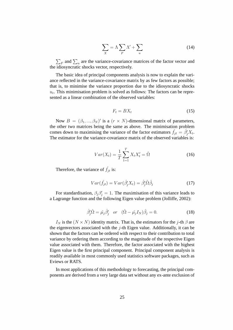
∑X
= Λ∑
F
Λ′ +∑
u
(14)
∑F and
∑u are the variance-covariance matrices of the factor vector and
the idiosyncratic shocks vector, respectively.
The basic idea of principal components analysis is now to explain the vari-ance reflected in the variance-covariance matrix by as few factors as possible;that is, to minimise the variance proportion due to the idiosyncratic shocksut. This minimisation problem is solved as follows: The factors can be repre-sented as a linear combination of the observed variables:
Ft = BXt (15)
Now B = (β1, ..., βN)′ is a (r × N)-dimensional matrix of parameters,the other two matrices being the same as above. The minimisation problemcomes down to maximising the variance of the factor estimatorsfjt = β′jXt.The estimator for the variance-covariance matrix of the observed variables is:
V ar(Xt) =1
T
T∑1=1
XtX′t = Ω (16)
Therefore, the variance offjt is:
V ar(fjt) = V ar(β′jXt) = β′jΩβj (17)
For standardisation,βjβ′j = 1. The maximisation of this variance leads to
a Lagrange function and the following Eigen value problem (Jolliffe, 2002):
β′jΩ = µjβ′j or (Ω− µjIN)βj = 0. (18)
IN is the(N ×N) identity matrix. That is, the estimators for thej-th β arethe eigenvectors associated with thej-th Eigen value. Additionally, it can beshown that the factors can be ordered with respect to their contribution to totalvariance by ordering them according to the magnitude of the respective Eigenvalue associated with them. Therefore, the factor associated with the highestEigen value is the first principal component. Principal component analysis isreadily available in most commonly used statistics software packages, such asEviews or RATS.
In most applications of this methodology to forecasting, the principal com-ponents are derived from a very large data set without any ex-ante exclusion of
25
data series; that is, including time series we know to be lagging GDP growth9.The idea is to identify the common factors that drive all the data and can bethought of as representing a business cycle. However, in the sections abovewe have come to the conclusion that a classic business cycle may be hard toidentify in Estonia. Therefore, we see principal components analysis ratheras another way of producing a dynamically weighted averaging of time seriesand we include time series which we already know have some sort of lead-ing relationship with the reference series together with some other variables tomake the sample more representative for the whole data set. A list of these 34variables can be found in the appendix. All series were made stationary andde-seasonalised (by taking fourth differences) when necessary. Finally, westandardised all series to mean zero and standard deviation unity. We estimatetwo different models:
• Specification 1: Including only contemporaneous values of the 31 timeseries.
• Specification 2: Including the first lag of all the time series included.Stock and Watson (2002) refer to this as a “stacked” data set; therefore,62 time series are included.
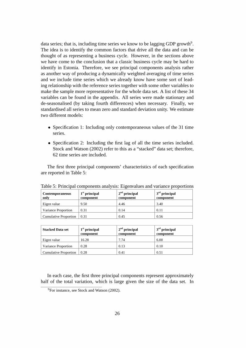
The first three principal components’ characteristics of each specificationare reported in Table 5:
Table 5: Principal components analysis: Eigenvalues and variance proportions
Contemporaneous only
1st principal component
2nd principal component
3rd principal component
Eigen value 9.50 4.46 3.40
Variance Proportion 0.31 0.14 0.11
Cumulative Proportion 0.31 0.45 0.56
Stacked Data set 1st principal component
2nd principal component
3rd principal component
Eigen value 16.28 7.74 6.00
Variance Proportion 0.28 0.13 0.10
Cumulative Proportion 0.28 0.41 0.51
In each case, the first three principal components represent approximatelyhalf of the total variation, which is large given the size of the data set. In
9For instance, see Stock and Watson (2002).
26
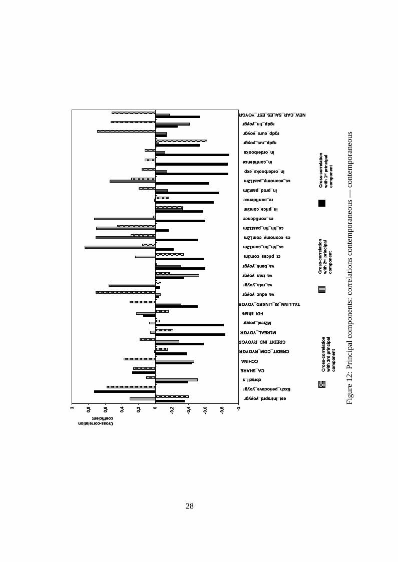
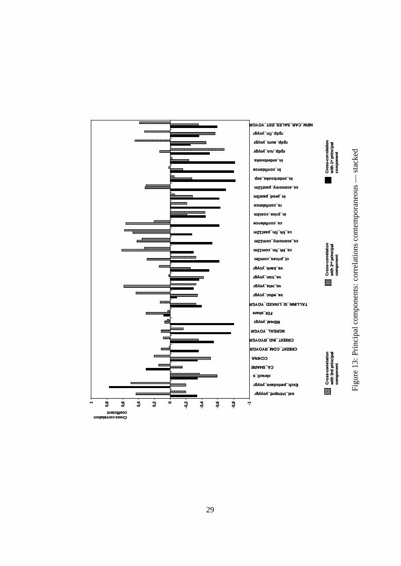
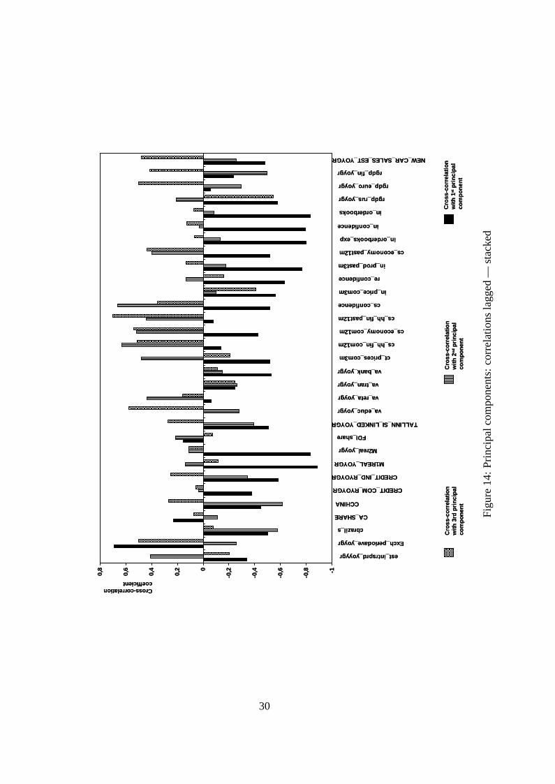
most applications of static principal components, a similar share of varianceis accounted for by the derived principal components; for example, Eickmeierand Breitung (2005), Marcellino, Stock and Watson (2000), and Altissimo etal. (2001), who all find a range between 32% and 55%. Correlations betweenderived principal components and the input series can be seen in the follow-ing three figures. Figure 12 displays correlation coefficients between the inputdata series and the principal components derived from the contemporaneousdata set (specification 1). Figure 13 displays correlation coefficients betweenthe contemporaneous input data series and principal components derived fromthe stacked data set (specification 2), and Figure 14 displays correlation coef-ficients between the lagged input data series and principal components derivedfrom the stacked data set (specification 2). A similar representation is used byStock and Watson (2002).
27
Cro
ss-c
orr
elat
ion
w
ith
1st
pri
nci
pal
co
mp
on
ent
Cro
ss-c
orr
elat
ion
w
ith
2n
dp
rin
cip
al
com
po
nen
t
Cro
ss-c
orr
elat
ion
w
ith
3rd
pri
nci
pal
co
mp
on
ent
-1
-0,8
-0,6
-0,4
-0,20
0,2
0,4
0,6
0,81
est_intrsprd_yoyygr
Exch_periodave_yoygr
cbrazil_s
CA_SHARE
CCHINA
CREDIT_COM_RYOYGR
CREDIT_IND_RYOYGR
M1REAL_YOYGR
M2real_yoygr
FDI_share
TALLINN_SI_LINKED_YOYGR
va_educ_yoygr
va_reta_yoygr
va_tran_yoygr
va_bank_yoygr
ct_prices_com3m
cs_hh_fin_com12m
cs_economy_com12m
cs_hh_fin_past12m
cs_confidence
in_price_com3m
re_confidence
in_prod_past3m
cs_economy_past12m
in_orderbooks_exp
in_confidence
in_orderbooks
rgdp_rus_yoygr
rgdp_euro_yoygr
rgdp_fin_yoygr
NEW_CAR_SALES_EST_YOYGR
Cross-correlation coefficient
Cro
ss-c
orr
elat
ion
w
ith
1st
pri
nci
pal
co
mp
on
ent
Cro
ss-c
orr
elat
ion
w
ith
2n
dp
rin
cip
al
com
po
nen
t
Cro
ss-c
orr
elat
ion
w
ith
3rd
pri
nci
pal
co
mp
on
ent
-1
-0,8
-0,6
-0,4
-0,20
0,2
0,4
0,6
0,81
est_intrsprd_yoyygr
Exch_periodave_yoygr
cbrazil_s
CA_SHARE
CCHINA
CREDIT_COM_RYOYGR
CREDIT_IND_RYOYGR
M1REAL_YOYGR
M2real_yoygr
FDI_share
TALLINN_SI_LINKED_YOYGR
va_educ_yoygr
va_reta_yoygr
va_tran_yoygr
va_bank_yoygr
ct_prices_com3m
cs_hh_fin_com12m
cs_economy_com12m
cs_hh_fin_past12m
cs_confidence
in_price_com3m
re_confidence
in_prod_past3m
cs_economy_past12m
in_orderbooks_exp
in_confidence
in_orderbooks
rgdp_rus_yoygr
rgdp_euro_yoygr
rgdp_fin_yoygr
NEW_CAR_SALES_EST_YOYGR
Cross-correlation coefficient
Fig
ure
12:
Prin
cipa
lcom
pone
nts:
corr
elat
ions
cont
empo
rane
ous
—co
ntem
pora
neou
s
28
Cro
ss-c
orr
elat
ion
w
ith
1st
pri
nci
pal
co
mp
on
ent
Cro
ss-c
orr
elat
ion
w
ith
2n
dp
rin
cip
al
com
po
nen
t
Cro
ss-c
orr
elat
ion
w
ith
3rd
pri
nci
pal
co
mp
on
ent
-1
-0,8
-0,6
-0,4
-0,20
0,2
0,4
0,6
0,81
est_intrsprd_yoyygr
Exch_periodave_yoygr
cbrazil_s
CA_SHARE
CCHINA
CREDIT_COM_RYOYGR
CREDIT_IND_RYOYGR
M1REAL_YOYGR
M2real_yoygr
FDI_share
TALLINN_SI_LINKED_YOYGR
va_educ_yoygr
va_reta_yoygr
va_tran_yoygr
va_bank_yoygr
ct_prices_com3m
cs_hh_fin_com12m
cs_economy_com12m
cs_hh_fin_past12m
cs_confidence
in_price_com3m
re_confidence
in_prod_past3m
cs_economy_past12m
in_orderbooks_exp
in_confidence
in_orderbooks
rgdp_rus_yoygr
rgdp_euro_yoygr
rgdp_fin_yoygr
NEW_CAR_SALES_EST_YOYGR
Cross-correlation coefficient
Cro
ss-c
orr
elat
ion
w
ith
1st
pri
nci
pal
co
mp
on
ent
Cro
ss-c
orr
elat
ion
w
ith
2n
dp
rin
cip
al
com
po
nen
t
Cro
ss-c
orr
elat
ion
w
ith
3rd
pri
nci
pal
co
mp
on
ent
-1
-0,8
-0,6
-0,4
-0,20
0,2
0,4
0,6
0,81
est_intrsprd_yoyygr
Exch_periodave_yoygr
cbrazil_s
CA_SHARE
CCHINA
CREDIT_COM_RYOYGR
CREDIT_IND_RYOYGR
M1REAL_YOYGR
M2real_yoygr
FDI_share
TALLINN_SI_LINKED_YOYGR
va_educ_yoygr
va_reta_yoygr
va_tran_yoygr
va_bank_yoygr
ct_prices_com3m
cs_hh_fin_com12m
cs_economy_com12m
cs_hh_fin_past12m
cs_confidence
in_price_com3m
re_confidence
in_prod_past3m
cs_economy_past12m
in_orderbooks_exp
in_confidence
in_orderbooks
rgdp_rus_yoygr
rgdp_euro_yoygr
rgdp_fin_yoygr
NEW_CAR_SALES_EST_YOYGR
Cross-correlation coefficient
Fig
ure
13:
Prin
cipa
lcom
pone
nts:
corr
elat
ions
cont
empo
rane
ous
—st
acke
d
29
Cro
ss-c
orr
elat
ion
w
ith
1st
pri
nci
pal
co
mp
on
ent
Cro
ss-c
orr
elat
ion
w
ith
2n
dp
rin
cip
al
com
po
nen
t
Cro
ss-c
orr
elat
ion
w
ith
3rd
pri
nci
pal
co
mp
on
ent
-1
-0,8
-0,6
-0,4
-0,20
0,2
0,4
0,6
0,8
est_intrsprd_yoyygr
Exch_periodave_yoygr
cbrazil_s
CA_SHARE
CCHINA
CREDIT_COM_RYOYGR
CREDIT_IND_RYOYGR
M1REAL_YOYGR
M2real_yoygr
FDI_share
TALLINN_SI_LINKED_YOYGR
va_educ_yoygr
va_reta_yoygr
va_tran_yoygr
va_bank_yoygr
ct_prices_com3m
cs_hh_fin_com12m
cs_economy_com12m
cs_hh_fin_past12m
cs_confidence
in_price_com3m
re_confidence
in_prod_past3m
cs_economy_past12m
in_orderbooks_exp
in_confidence
in_orderbooks
rgdp_rus_yoygr
rgdp_euro_yoygr
rgdp_fin_yoygr
NEW_CAR_SALES_EST_YOYGR
Cross-correlation coefficient
Cro
ss-c
orr
elat
ion
w
ith
1st
pri
nci
pal
co
mp
on
ent
Cro
ss-c
orr
elat
ion
w
ith
2n
dp
rin
cip
al
com
po
nen
t
Cro
ss-c
orr
elat
ion
w
ith
3rd
pri
nci
pal
co
mp
on
ent
-1
-0,8
-0,6
-0,4
-0,20
0,2
0,4
0,6
0,8
est_intrsprd_yoyygr
Exch_periodave_yoygr
cbrazil_s
CA_SHARE
CCHINA
CREDIT_COM_RYOYGR
CREDIT_IND_RYOYGR
M1REAL_YOYGR
M2real_yoygr
FDI_share
TALLINN_SI_LINKED_YOYGR
va_educ_yoygr
va_reta_yoygr
va_tran_yoygr
va_bank_yoygr
ct_prices_com3m
cs_hh_fin_com12m
cs_economy_com12m
cs_hh_fin_past12m
cs_confidence
in_price_com3m
re_confidence
in_prod_past3m
cs_economy_past12m
in_orderbooks_exp
in_confidence
in_orderbooks
rgdp_rus_yoygr
rgdp_euro_yoygr
rgdp_fin_yoygr
NEW_CAR_SALES_EST_YOYGR
Cross-correlation coefficient
Fig
ure
14:
Prin
cipa
lcom
pone
nts:
corr
elat
ions
lagg
ed—
stac
ked
30
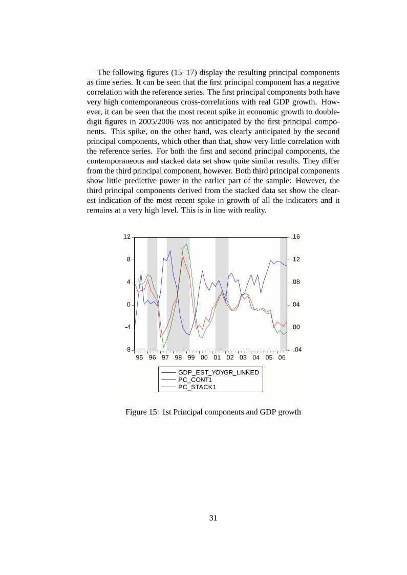
The following figures (15–17) display the resulting principal componentsas time series. It can be seen that the first principal component has a negativecorrelation with the reference series. The first principal components both havevery high contemporaneous cross-correlations with real GDP growth. How-ever, it can be seen that the most recent spike in economic growth to double-digit figures in 2005/2006 was not anticipated by the first principal compo-nents. This spike, on the other hand, was clearly anticipated by the secondprincipal components, which other than that, show very little correlation withthe reference series. For both the first and second principal components, thecontemporaneous and stacked data set show quite similar results. They differfrom the third principal component, however. Both third principal componentsshow little predictive power in the earlier part of the sample: However, thethird principal components derived from the stacked data set show the clear-est indication of the most recent spike in growth of all the indicators and itremains at a very high level. This is in line with reality.
-8
-4
0
4
8
12
-.04
.00
.04
.08
.12
.16
95 96 97 98 99 00 01 02 03 04 05 06
GDP_EST_YOYGR_LINKEDPC_CONT1PC_STACK1
Figure 15: 1st Principal components and GDP growth
31

-6
-4
-2
0
2
4
6
-.04
.00
.04
.08
.12
.16
.20
95 96 97 98 99 00 01 02 03 04 05 06
GDP_EST_YOYGR_LINKEDPC_CONT2PC_STACK2
Figure 16: 2nd Principal components and GDP growth
-6
-4
-2
0
2
4
6
8
10
-.08
-.04
.00
.04
.08
.12
.16
.20
.24
95 96 97 98 99 00 01 02 03 04 05 06
GDP_EST_YOYGR_LINKEDPC_CONT3PC_STACK3
Figure 17: 3rd Principal components and GDP growth
32
It remains to be answered which principal components should be includedwhen trying to forecast economic growth. An often used criterion for deter-mining the optimal number of factors is the test developed by Bai and Ng(2002), which was explicitly developed for this kind of approximate commonfactor model using static principal components and relying upon the variance-covariance matrix of the data set10. Another possibility would be to simplycompare the forecasting performance of the models11. As the number of timeseries is rather limited here, we will not consider more than three principal-components-based common factors for each data set and will follow the fore-cast evaluation approach. We estimated the regressions of the reference serieson all possible combinations of the principal components derived from thecontemporaneous data set and the stacked data set, respectively. The fittedcoefficients were used to run forecasts over the whole sample period 1995:1to 2006:1 and estimate the root mean squared forecasting error (RMSFE), de-fined as follows:
RMSFE =
√√√√ T+h∑t=T+1
(yt − yt)2/h (19)
It turns out that for both cases, the inclusion of all three principal compo-nents yields the best forecast, even though the inclusion of only the first twois only slightly worse. When we go on to compare state-space modelling andprincipal components in the next section, we will keep two principal compo-nents based models:
• Three principal components derived from the contemporaneous data set.
• Three principal components derived from the stacked data set.
5. Forecast comparison
In the following section we use tests developed by Diebold and Mariano(1995) and Clark and McCracken (2001) to carry out comparisons of the in-sample and out-of-sample performances of the developed indicators, respec-tively. For a discussion of the merits of different tests and methods see Chen(2005).
One simple way of in-sample performance testing is to compare the F-tests from regressing the reference series on different specifications involving
10See Breitung and Eickmeier (2005).11See Stock and Watson (2002).
33
the various leading indicators. However, this will not permit any statementas to whether the difference between the two forecasting models is actuallysignificant. Diebold and Mariano (1995) have developed a method that doesexactly that — they simply regress the difference between the absolute forecasterrors of both series on a constant using robust standard errors and check thet-value of the constant.
We will compare five specifications, of which the naïve AR(1) model ofreal GDP growth (20) will serve as the benchmark model. Note that we usestatic fitted forecasts. This means that each quarter the actual value of GDPgrowth is multiplied by the fitted regression coefficients rather than using afitted value of GDP growth. This is done for all specifications. The naïvemodel is defined as follows:
gdpt = cnaive + bnaive · gdpt−1 + enaive (20)
We include the lagged dependent variable in the two different specificationsof the state-space-model-forecasts as well:
gdpt = cind 3 S + bind 3 S · gdpt−1 + bind 3 S · iind 3 S,t−1 + eind 3 S (21)
gdpt = ci0 m1 tsi+bi0 m1 tsi ·gdpt−1+bi0 m1 tsi ·ii0 m1 tsi,t−1+ei0 m1 tsi (22)
Finally, as mentioned in the section above, we use the first three principalcomponents derived from the contemporaneous data set and the stacked dataset, respectively. Again, we include lagged values of the dependent variableand use static forecasting.
gdpt = c PC,Cont + b PC1,Cont · gdpt−1 + b PC1,Cont · PC 1,Cont,t−1 ++ b PC2,Cont · PC 2,Cont,t−1 + b PC3,Cont · PC 3,Cont,t−1 + e PC,Cont (23)
gdpt = c PC,Stack + b PC1,Stack · gdpt−1 + b PC1,Stack · PC 1,Stack,t−1 ++ b PC2,Stack · PC 2,Stack,t−1 + b PC3,Stack · PC 3,Stack,t−1 + e PC,Stack (24)
The RATS-procedure we used to implement the Diebold and Mariano testreports the p-values for the t-test on the constant; that is, a small p-value indi-cates that the alternative performs better than the benchmark. The followingtable reports the p-values for different specifications and periods.
34
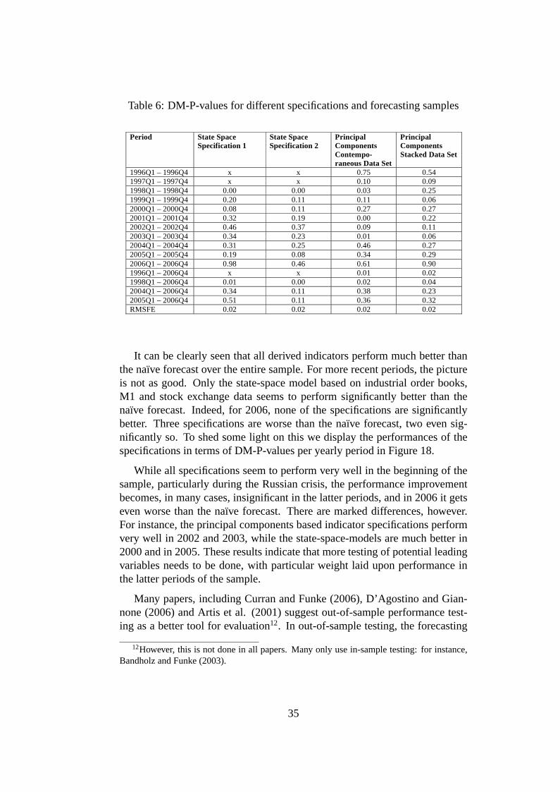
Table 6: DM-P-values for different specifications and forecasting samples
Period State Space Specification 1
State Space Specification 2
Principal Components Contempo-raneous Data Set
Principal Components Stacked Data Set
1996Q1 – 1996Q4 x x 0.75 0.54 1997Q1 – 1997Q4 x x 0.10 0.09 1998Q1 – 1998Q4 0.00 0.00 0.03 0.25 1999Q1 – 1999Q4 0.20 0.11 0.11 0.06 2000Q1 – 2000Q4 0.08 0.11 0.27 0.27 2001Q1 – 2001Q4 0.32 0.19 0.00 0.22 2002Q1 – 2002Q4 0.46 0.37 0.09 0.11 2003Q1 – 2003Q4 0.34 0.23 0.01 0.06 2004Q1 – 2004Q4 0.31 0.25 0.46 0.27 2005Q1 – 2005Q4 0.19 0.08 0.34 0.29 2006Q1 – 2006Q4 0.98 0.46 0.61 0.90 1996Q1 – 2006Q4 x x 0.01 0.02 1998Q1 – 2006Q4 0.01 0.00 0.02 0.04 2004Q1 – 2006Q4 0.34 0.11 0.38 0.23 2005Q1 – 2006Q4 0.51 0.11 0.36 0.32 RMSFE 0.02 0.02 0.02 0.02
It can be clearly seen that all derived indicators perform much better thanthe naïve forecast over the entire sample. For more recent periods, the pictureis not as good. Only the state-space model based on industrial order books,M1 and stock exchange data seems to perform significantly better than thenaïve forecast. Indeed, for 2006, none of the specifications are significantlybetter. Three specifications are worse than the naïve forecast, two even sig-nificantly so. To shed some light on this we display the performances of thespecifications in terms of DM-P-values per yearly period in Figure 18.
While all specifications seem to perform very well in the beginning of thesample, particularly during the Russian crisis, the performance improvementbecomes, in many cases, insignificant in the latter periods, and in 2006 it getseven worse than the naïve forecast. There are marked differences, however.For instance, the principal components based indicator specifications performvery well in 2002 and 2003, while the state-space-models are much better in2000 and in 2005. These results indicate that more testing of potential leadingvariables needs to be done, with particular weight laid upon performance inthe latter periods of the sample.
Many papers, including Curran and Funke (2006), D’Agostino and Gian-none (2006) and Artis et al. (2001) suggest out-of-sample performance test-ing as a better tool for evaluation12. In out-of-sample testing, the forecasting
12However, this is not done in all papers. Many only use in-sample testing: for instance,Bandholz and Funke (2003).
35

0
0,2
0,4
0,6
0,8
1
1998 1999 2000 2001 2002 2003 2004 2005 2006
P-Value for Forecast better than naive forecast
Forecasting Horizon
State Space• Industrial Orderbooks,
M1 and Tallinn Stock Exchange Index
State Space• Industrial Orderbooks,
M1 and Loans to Individuals
Principal Components• Contemporaneous
dataset
Principal Components• Stacked dataset
Figure 18: Forecasting Performance: DM-P-Values per period
model is estimated for a sub-sample of the entire available sample and thenforecasts for the remaining sample are evaluated with respect to the actual val-ues. We perform test procedures used by Clark and McCracken (2001) usingthe same nested forecasting model specifications as in (20) through (24), with(20) again serving as the benchmark model. Four different statistics are sug-gested by Clark and McCracken: the two MSE (mean squared error) statisticstest for equal forecasting accuracy. The MSE-t test was proposed by Grangerand Newbold (1977), while critical values for the MSE-f test were provided byMcCracken (1999). The ENC (encompassing) statistics test for the benchmarkmodel encompasses the alternative. The ENC-T test is described in Clark andMcCracken (2001) and draws from Diebold and Mariano (1995) and Harveyet al. (1998). The ENC-f test was developed by Clark and McCracken (2001)and uses variance weighting to improve the small-sample performance of theencompassing test.
Again, the results are mixed (see Table 7). We will not pay much attentionto the equal MSE-tests, as they only confirm what has already been shownby the in-sample tests; namely, that 2006 was a particularly bad year for allthe different forecasting models compared to the naïve model. However, ex-cept for the principal-components-based model based on the stacked data set,for almost all other forecasting horizons, the indicators do reveal additionalinformation: that is, they are not already encompassed by the naïve model.
36
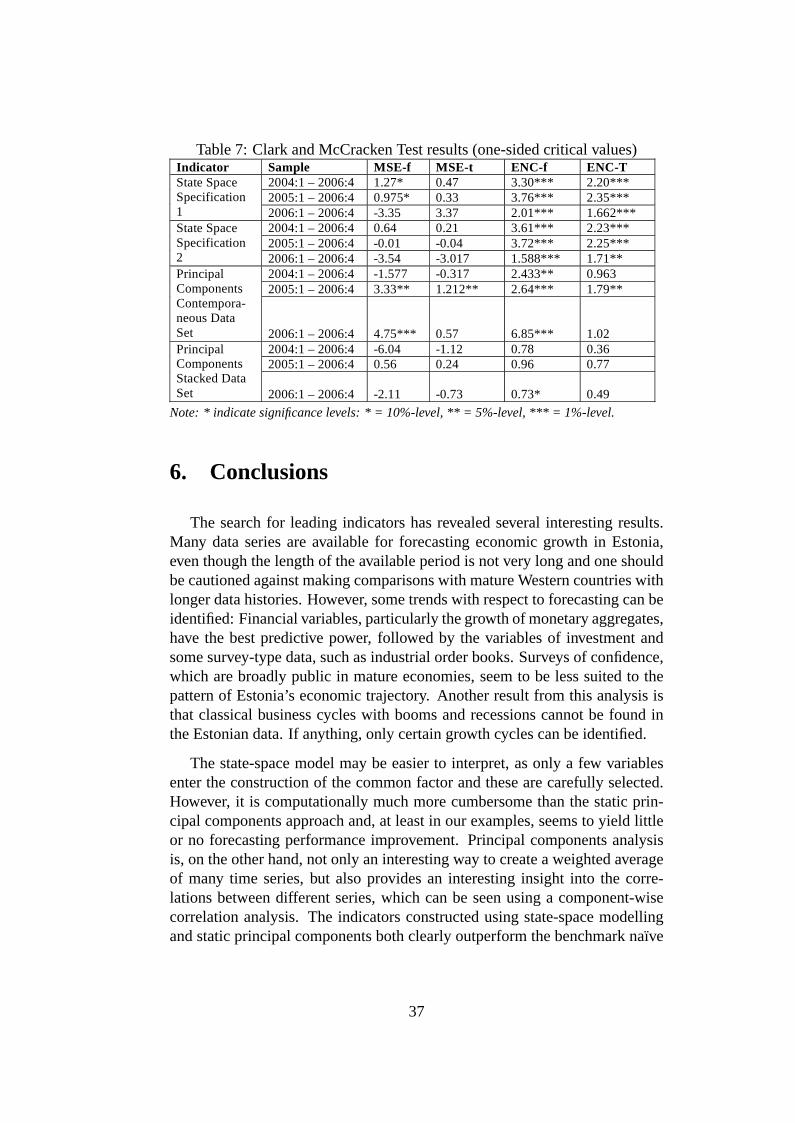
Table 7: Clark and McCracken Test results (one-sided critical values)Indicator Sample MSE-f MSE-t ENC-f ENC-T
2004:1 – 2006:4 1.27* 0.47 3.30*** 2.20*** 2005:1 – 2006:4 0.975* 0.33 3.76*** 2.35***
State Space Specification 1 2006:1 – 2006:4 -3.35 3.37 2.01*** 1.662***
2004:1 – 2006:4 0.64 0.21 3.61*** 2.23*** 2005:1 – 2006:4 -0.01 -0.04 3.72*** 2.25***
State Space Specification 2 2006:1 – 2006:4 -3.54 -3.017 1.588*** 1.71**
2004:1 – 2006:4 -1.577 -0.317 2.433** 0.963 2005:1 – 2006:4 3.33** 1.212** 2.64*** 1.79**
Principal Components Contempora-neous Data Set
2006:1 – 2006:4
4.75***
0.57
6.85***
1.02
2004:1 – 2006:4 -6.04 -1.12 0.78 0.36 2005:1 – 2006:4 0.56 0.24 0.96 0.77
Principal Components Stacked Data Set
2006:1 – 2006:4
-2.11
-0.73
0.73*
0.49
Note: * indicate significance levels: * = 10%-level, ** = 5%-level, *** = 1%-level.
6. Conclusions
The search for leading indicators has revealed several interesting results.Many data series are available for forecasting economic growth in Estonia,even though the length of the available period is not very long and one shouldbe cautioned against making comparisons with mature Western countries withlonger data histories. However, some trends with respect to forecasting can beidentified: Financial variables, particularly the growth of monetary aggregates,have the best predictive power, followed by the variables of investment andsome survey-type data, such as industrial order books. Surveys of confidence,which are broadly public in mature economies, seem to be less suited to thepattern of Estonia’s economic trajectory. Another result from this analysis isthat classical business cycles with booms and recessions cannot be found inthe Estonian data. If anything, only certain growth cycles can be identified.
The state-space model may be easier to interpret, as only a few variablesenter the construction of the common factor and these are carefully selected.However, it is computationally much more cumbersome than the static prin-cipal components approach and, at least in our examples, seems to yield littleor no forecasting performance improvement. Principal components analysisis, on the other hand, not only an interesting way to create a weighted averageof many time series, but also provides an interesting insight into the corre-lations between different series, which can be seen using a component-wisecorrelation analysis. The indicators constructed using state-space modellingand static principal components both clearly outperform the benchmark naïve
37

AR(1) model in in-sample testing. However, this seems to be due to a verystrong performance in the earlier part of the sample, particularly during theRussian crisis. The performance in the latter part of the sample, particularlyin 2006, seems to be rather poor, which is confirmed by out-of-sample testing.This might be due to a systemic change; that is, factors other than the financialvariables we identified might have taken over the driving of economic devel-opment in Estonia. However, this could also be a temporary break.
38
References
Altissimo, F., Bassanetti, A., Cristadoro, R., Forni, M., Hallin, M., Lippi, M.and Reichlin, L., 2001. EuroCOIN: a real time coincident indicator of the euroarea business cycle. CEPR Working Paper 3108.
Artis, M., Banerjee, A. and Marcellino, M., 2001. Factor Forecasts for theUK. EUI Working Paper No. 2001/15.
Bai, J. and Ng, S., 2002. Determining the number of factors in approximatefactor models. Econometrica 70:191–221.
Bandholz, H., 2004. Konjunkturelle Frühindikatoren für die BundesrepublikDeutschland und die Freie und Hansestadt Hamburg. Frankfurt am Main: Pe-ter Lang.
Bandholz, H. and Funke, M., 2003. In Search of Leading Indicators of Eco-nomic Activity in Germany. Journal of Forecasting 22:277–297.
Breitung, J. and Eickmeier, S., 2005. Dynamic factor models. Deutsche Bun-desbank Discussion Paper.
Bry, G. and Boschan, C., 1971. Cyclical Analysis of Time Series: SelectedProcedures and Computer Programs. In National Bureau of Economic Re-search. New York.
CESIfo, 2007. World Economic Survey. Vol. 6. CESIfo, No. 4.
Chen, S.-S., 2005. A Note on In-Sample and Out-of-Sample Tests for GrangerCausality. Journal of Forecasting, No. 24:453–464.
Clark, T. E. and McCracken, M. W., 2001. Tests of Forecast Accuracy andEncompassing for Nested Models. Journal of Econometrics, No. 105:85–110.
Curran, D. and Funke, M., 2006. Taking the temperature — forecasting GDPgrowth for mainland China. BOFIT Discussion Papers, No. 6.
D’Agostino, A. and Giannone, D., 2006. Comparing alternative predictorsbased on large-panel factor models. ECB Working Paper Series.
Diebold, F. X. and Mariano, R. S., 1995. Comparing predictive accuracy.Journal of Business Economic Statistics, No. 13:253–263.
Dreger, C. and Schuhmacher, C., 2004. Estimating Large-Scale Factor Modelsfor Economic Activity in Germany: Do They Outperform Simpler Models?Jahrbücher für Nationalökonomie und Statistik, No. 224:731–750.
39
Eickmeier, S. and Breitung, J., 2005. How synchronized are Central and EastEuropean economies with the euro area? Evidence from a structural factormodel. Bundesbank Discussion Paper Series 1: Economic Studies.
Estrella, A. and Mishkin, F. S., 1998. Predicting U.S. Recessions: FinancialVariables as Leading Indicators. The Review of Economics and Statistics, No.80:45–61.
Forni, M., Hallin, M. and Lippi, M., 2003. The Generalized Dynamic FactorModel one-sided estimation and forecasting. Journal of the American Statisti-cal Association.
Forni, M., Hallin, M., Lippi, M. and Reichlin, L., 2001. Coincident and lead-ing indicators for the Euro area. The Economic Journal.
Forni, M., Lippi, M. and Reichlin, L., 2000. The Generalized Factor Model:Identification and Estimation. The Review of Economics and Statistics, No.82:540–554.
Fritsche, U. and Stephan, S., 2000. Leading Indicators of German Busi-ness Cycles: an Assessment of Properties. Deutsches Institut für Wirtschafts-forschung (DIW), Berlin.
G. C. o. E. E. (Sachverständigenrat),(2005). Annual Report 2003/2004.
Gerlach, S. and Yiu, M. S., 2005. A dynamic factor model of economic activ-ity in Hong Kong. Pacific Economic Review, No. 10:279–292.
Granger, C. W. J. and Newbold, P., 1977. Forecasting Economic Time Series.Orlando: Academic Press.
Harvey, D. I., Leybourne, S. J. and Newbold, P., 1998. Tests for ForecastEncompassing. Journal of Business Economic Statistics, No. 16:254–259.
Jolliffe, I. T., 2002. Principal Component Analysis. New York: Springer.
Kalman, R. E., 1960. A New Approach to Linear Filtering and PredictionProblems. Journal of Basic Engineering, Transactions of the ASME, Series D.
Kalman, R. E., 1963. New Methods in Wiener Filtering Theory. In Proceed-ings of the First Symposium of Engineering Applications of Random FunctionTheory and Probability. (Eds, Bogdanoff, J. L. and Kozin, F.). New York: Wi-ley, 270–388.
40

Kapetanios, G. and Marcellino, M., 2006. Impulse Response Functions fromStructural Dynamic Factor Models: A Monte Carlo Evaluation. CEPR Dis-cussion Paper, No. 5621.
Kim, C.-J., 1999. State-space models with regime switching: classical andGibbs-sampling approaches with applications. Cambridge, Mass.: MIT Press.
Marcellino, M., Stock, J. H. and Watson, M. W., 2000. A dynamic factoranalysis of EMU.
McCracken, M. W., 1999. Asymptotics for out-of-sample tests of causality.Louisiana State University.
Nerb, G., 2007. The Importance of Representative Surveys of Enterprises forEmpirically Oriented Business Cycle Research. In Handbook of Survey-BasedBusiness Cycle Analysis (Ed, Goldrian, G.). Cheltenham: Edward Elgar.
Stock, J. H. and Watson, M. W., 1991. A Probability Model of the CoincidentEconomic Indicators. In Leading Indicators: New Approaches and Forecast-ing Records (Eds, Lahiri, K. and Moore, G. H.). Cambridge, UK: CambridgeUniversity Press, 63–89.
Stock, J. H. and Watson, M. W., 2002. Forecasting Using Principal Compo-nents from a Large Panel of Predictors. Journal of the American StatisticalAssociation, No. 97:147–162.
Zanghieri, P., 2006. Current account dynamics in the new Member States. InThe Central and Eastern European Countries and the European Union (Eds,Artis, M., Banerjee, A. and Marcellino, M.). Cambridge: Cambridge Univer-sity Press, 245–273.
41
Appendix 1. Data set and cross correlations
No. Name of Series Transformation ADF (p-value)
Max X-corr
at lag (-lead)
1 Assets with BIS-reporting banks
YOY change 0.00 0.16 0
2 Brazilian Stock Market Index YOY change 0.01 0.45 2 3 Chinese Stock Market Index YOY change 0.22 -0.26 -4
4 Commercial banks' foreign assets
YOY change 0.00 0.31 2
5 Commercial banks' foreign liabilities
YOY change 0.33 0.24 1
6 Construction building activity over the past 3 months
YOY change 0.00 0.43 1
7 Construction confidence indicator
YOY change 0.00 0.46 -1
8 Construction employment over the next 3 months
YOY change 0.01 0.39 1
9
Construction factors limiting building activity ** insufficient demand
YOY change 0.01 -0.44 1
10
Construction factors limiting building activity ** weather conditions
YOY change 0.00 0.33 2
11 Construction order books YOY change 0.17 0.50 -1
12 Construction prices over the next 3 months
YOY change 0.18 0.53 0
13 Consumer confidence Indicator YOY change 0.11 0.55 0
14
Consumer financial situation of households over next 12 months
YOY change 0.01 0.34 -1
15 Consumer financial situation of households over past 12 months
YOY change 0.00 0.31 -3
16 Consumer major purchases over next 12 months
YOY change 0.01 0.33 -1
17 Consumer perception of change in unemployment
YOY change 0.11 -0.58 0
18
Consumer perception of general economic situation over next 12 months
YOY change 0.01 0.38 1
19
Consumer perception of general economic situation over past 12 months
YOY change 0.00 0.52 1
20 Consumer price index (av) YOY change 0.01 -0.26 3
21 Consumer price Index at end of period
YOY change 0.00 -0.21 0
22 Current Account share of GDP Levels, de-seasonalised
0.00 -0.52 -2
23 Current-Account balance YOY change 0.00 0.33 1 24 Deposit interest rate YOY change 0.00 0.68 -2 25 Economic sentiment indicator YOY change 0.20 0.60 0 26 Estonian interest rate spread YOY change 0.00 0.28 0 27 Euro zone real GDP YOY change 0.05 -0.35 4 29 FDI as share of GDP Levels 0.00 0.27 -3 30 Finnish exports YOY change 0.38 -0.22 4
42

No. Name of Series Transformation ADF (p-value)
Max X-corr
at lag (-lead)
31 Finnish imports YOY change 0.14 0.15 2 32 Finnish Real GDP YOY change 0.00 -0.31 4
33 Foreign direct investment Change yoy
YOY change 0.00 0.25 2
34 Foreign-exchange reserves YOY change 0.05 0.30 -2 35 Estonian Real GDP change YOY change 0.06 1.00 0 36 Gold, national valuation YOY change 0.87 0.29 1 37 Industrial confidence indicator YOY change 0.03 0.58 1
38 Industrial current export order books
YOY change 0.00 0.54 1
39 Industrial current overall order books
YOY change 0.00 0.60 1
40 Industrial current stock of finished products
YOY change 0.00 -0.46 0
41 Industrial production index YOY change 0.00 0.84 0
42 Industrial production over the past 3 months
YOY change 0.02 0.49 2
43 Industrial production will over the next 3 months
YOY change 0.00 0.27 1
44 Industrial selling prices will over the next 3 months
YOY change 0.01 0.39 4
45 International reserves YOY change 0.05 0.30 -2 46 Lending interest rate (%) YOY change 0.00 0.67 -3
47 Liabilities with BIS-reporting banks
YOY change 0.37 0.41 -1
48 Loan Stock granted to commercial undertakings
YOY real change 0.40 0.51 0
49 Loan Stock granted to individuals
YOY real change 0.14 0.58 1
50 Money market interest rate (%) YOY change 0.11 0.49 -1 51 Net taxes on products YOY change 0.02 0.80 0 52 New Car Registrations YOY change 0.02 0.56 0
53 Real effective exchange rate of the kroon
YOY change 0.01 -0.60 0
54 Retail Confidence indicator YOY change 0.00 0.47 1
55 Retail Employment over the next 3 months
YOY change 0.00 0.52 0
56
Retail orders placed with suppliers during the next 3 months
YOY change 0.00 0.47 0
57 Retail Stocks YOY change 0.00 0.30 -3 58 Russian GDP YOY real change 0.01 0.35 0 59 Stock of money M1 YOY real change 0.02 0.71 1 60 Stock of money M2 YOY real change 0.01 0.68 0
43
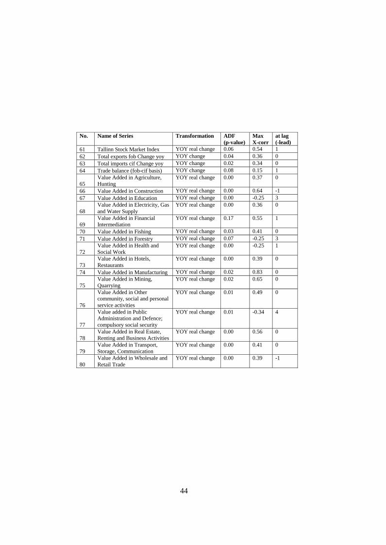
No. Name of Series Transformation ADF (p-value)
Max X-corr
at lag (-lead)
61 Tallinn Stock Market Index YOY real change 0.06 0.54 1 62 Total exports fob Change yoy YOY change 0.04 0.36 0 63 Total imports cif Change yoy YOY change 0.02 0.34 0 64 Trade balance (fob-cif basis) YOY change 0.08 0.15 1
65 Value Added in Agriculture, Hunting
YOY real change 0.00 0.37 0
66 Value Added in Construction YOY real change 0.00 0.64 -1 67 Value Added in Education YOY real change 0.00 -0.25 3
68 Value Added in Electricity, Gas and Water Supply
YOY real change 0.00 0.36 0
69 Value Added in Financial Intermediation
YOY real change 0.17 0.55 1
70 Value Added in Fishing YOY real change 0.03 0.41 0 71 Value Added in Forestry YOY real change 0.07 -0.25 3
72 Value Added in Health and Social Work
YOY real change 0.00 -0.25 1
73 Value Added in Hotels, Restaurants
YOY real change 0.00 0.39 0
74 Value Added in Manufacturing YOY real change 0.02 0.83 0
75 Value Added in Mining, Quarrying
YOY real change 0.02 0.65 0
76
Value Added in Other community, social and personal service activities
YOY real change 0.01 0.49 0
77
Value added in Public Administration and Defence; compulsory social security
YOY real change 0.01 -0.34 4
78 Value Added in Real Estate, Renting and Business Activities
YOY real change 0.00 0.56 0
79 Value Added in Transport, Storage, Communication
YOY real change 0.00 0.41 0
80 Value Added in Wholesale and Retail Trade
YOY real change 0.00 0.39 -1
44

Appendix 2. Principal components: time series in-cluded
No. Series Name Short name Type 1 Interest rate spread (long-term
minus short-term) est_intrsprd_yoygr Finance 2 Effective exchange rate Exch_periodave_yoygr Finance 3 Brazilian stock exchange cbrazil_s Finance 4 Current account as share of
GDP CA_SHARE Finance 5 Chinese stock exchange CCHINA Finance 6 Loans to Commercial
Customers CREDIT_COM_RYOYGR Finance 7 Loans to Individuals CREDIT_IND_RYOYGR Finance 8 Real Money Supply M1 M1REAL_YOYGR Finance 9 Real Money Supply M2 M2REAL_YOYGR Finance 10 Foreign Direct Investment (%
of GDP) FDI_share Finance 11 Tallinn stock exchange TALLINN_SI_LINKED_YOYGR Finance 12 Value added in Education va_educ_yoygr Sector 13 Value added in retail and
wholesale trade va_reta_yoygr Sector 14 Value added in
Transportation, etc. va_tran_yoygr Sector 15 Value added in Financial
Intermediation va_bank_yoygr Sector 16 Construction Prices over next
three months ct_prices_com3m Survey 17 Households’ financial
situation over next twelve months cs_hh_fin_com12m Survey
18 Households’ expectations of the state of the economy over next twelve months cs_economy_com12m Survey
19 Households’ financial situation over last twelve months cs_hh_fin_past12m Survey
20 Consumer confidence cs_confidence Survey 21 Manufacturing Prices over
next twelve months in_price_com3m Survey 22 Retail trade confidence re_confidence Survey 23 Industrial production over last
three months in_prod_past3m Survey 24 Consumers’ perception of the
state of the economy over last twelve months cs_economy_past12m Survey
25 Industrial order books, exports in_orderbooks_exp Survey
26 Industrial confidence in_confidence Survey 27 Industrial order books, overall in_orderbooks Survey 28 Russian real GDP rgdp_rus_yoygr Trade 29 Euro zone real GDP rgdp_euro_yoygr Trade 30 Finnish real GDP rgdp_fin_yoygr Trade 31 New car sales NEW_CAR_SALES_EST_YOY
GR Trade
45