Chapter 12 Small-Scale Winds

The phone rings in the office of a government meteorologist. The caller asks,

what were the wind conditions at a spot along a road at a certain time on a day many

months ago? The reason for the question: the caller was moving his new dishwasher in

the back of his pickup truck when it blew off the truck and was destroyed. The caller

wants specific weather information proving to the insurance company that a gust of wind

did in his dishwasher.

The meteorologist is perplexed. She knows that even in today’s high-tech world

we simply do not have weather information on the kind of small time and space scales the

caller wants. Furthermore, we also don’t have as good an understanding of winds on

small scales as we do on large scales. Ironically, meteorologists comprehend more

about the winds in an extratropical cyclone or a hurricane than they do about the local

winds that blow in our faces every day! The meteorologist tells the caller, “I’m sorry,

the best we can do is an hourly observation of winds thirty miles away from the scene of

the disaster.” Privately, she thinks that a tractor-trailer rig that blew past the pickup

probably played a role in the dishwasher’s demise. But she can’t quite know for sure.

In this chapter we tackle the topic of small-scale winds. For our purposes,

“small-scale” means winds that occur in a timespan you can perceive (usually minutes

or hours) and across distances you can see (often a few tens of miles or so). This is the

great frontier of meteorology, because so little is known about weather on these

dimensions. It’s not for lack of trying; as we’ll see, it is simply a fact of the atmosphere

that when meteorologists have to “sweat the small details,” they end up perspiring a

12-1

whole lot! Such is the maddening difficulty of small-scale meteorology, the gentle

breezes and the sudden windstorms that defy explanation.

Two unifying principles guide our study of these bedeviling winds. These

principles are the balance of forces we learned about in Chapter 6 and the geographic

features of the local landscape. For all of their complexity, small-scale winds generally

boil down to the interaction between a relatively strong pressure gradient and whatever

is in its way—a mountain, a valley, a lake, a dusty plain, or even an airplane.

Because geography is so crucial in the way that small-scale winds develop, we

will take an American tour of local winds. We are, for once, justified in our bias toward

the United States. The diversity of America’s landscapes and meteorology creates a wide

assortment of winds, spanning most of the types observed worldwide. After a short

introduction to the messiness of turbulence, we will follow the sun and take an east-to-

west journey through America and its small-scale winds.

12-2

Scales of wind motion

From large to small and timeless to fleeting, the atmosphere presents a

remarkably rich array of detail (Figure 12.1). This is as true for its winds as for its

clouds.

It turns out that the largest scales of motion are also the most long-lived, and the

smallest are the most ephemeral. Wind patterns on the scale of the Hadley cell are called,

appropriately enough, planetary-scale. Circulations such as an extratropical cyclone are

called synoptic-scale, the word “synoptic” referring to the “seeing-together” nature of

weather maps. In other words, synoptic-scale patterns

are those that are easily seen on weather maps. This

chapter concerns itself with the next two categories of

wind motions. Mesoscale phenomena occur on scales of

tens of kilometers and a few hours. The microscale

consists of circulations just a few meters in size, or less,

that last a few minutes, or even just a few seconds, or less. Table 12.1 classifies the types

of atmospheric motion we’ve studied in previous chapters, and will study in this chapter.

This classification system, combined with our knowledge of forces from Chapter

6, gives us a powerful insight into the nature of winds. We learned in Chapter 6 that the

primary forces affecting the horizontal motion of parcel of air are the pressure gradient

force, the Coriolis force, the centrifugal force, and the frictional force. On planetary and

synoptic scales, all four of these forces can come into play.

For example, a hurricane is a sharply curved, intense low-pressure system near

the surface. It is on the small end of synoptic-scale patterns, but can be represented well

Atmospheric motion comes in four sizes from largest to smallest: planetary-scale (e.g., Hadley cell), synoptic-scale (extratropical cyclone), mesoscale (thunderstorm) and microscale (swirl of leaves). The lifetimes of these motions generally range from years (or more) at the largest scales, to seconds at the smallest.

12-3

on a weather map. The pressure in a hurricane changes greatly over a short distance, and

so the horizontal pressure gradient force is significant. The hurricane forms away from

the equator and lasts a week or two, so the Coriolis force is important. The curved

motion of the wind around the eye brings the centrifugal force into play. Finally, the

wind near the surface “feels” the effect of the land or ocean as it spirals into the

hurricane, and therefore friction is important.

In the case of small-scale winds, the “balance of powers” of forces is completely

different. Winds that cover small distances and last for only a fraction of a day do not

“feel” the Earth’s rotation. As a result, the Coriolis force is negligible in most cases.

An analogy with basketball is appropriate here. The pressure gradient force is

like a dominating shooter who is held in check by a defensive specialist, the Coriolis

force. If the Coriolis force is out of the “game,” as is true for small-scale winds, two

things can happen: other “players” can step up to fill the role of the Coriolis force, or

else the pressure gradient force can proceed unguarded and do as it pleases.

In real life, both of these outcomes are possible. Often, the pressure gradient goes

largely unchecked on small scales, and does as we learned it always wants to do: blow

from high toward low pressure. This imbalance of forces is the genesis for the small-

scale winds we study in this chapter. The reason for the wide variety of types of small-

scale winds is simple: in its headlong rush from high to low pressure, the wind interacts

with different types of geographical features in different ways. In a sense, this entire

chapter can be summarized in the word-equation PRESSURE GRADIENT +

GEOGRAPHY = SMALL-SCALE WINDS.

12-4

That’s not the whole story, however. In many circumstances, particularly at the

smallest scales, other forces do step up and keep the pressure gradient force from acting

alone. This is particularly true of the frictional force. To understand the true role of

friction in small-scale winds, we need to explore the hair-raising and sometimes bone-

breaking subject known as “turbulence.”

Friction in the air: Turbulent “eddies”

Friction is a familiar concept to us: sandpaper, tread on tires and tennis shoes,

striking a match. All of these examples involve one rough surface coming into contact

with another. Air, however, doesn’t have any rough surfaces. How, then, is there any

friction? We took it on faith in Chapter 6, but now is the time to explore the concept

more fully.

The friction in a fluid, such as air, is called viscosity. You hear this word on TV

in relation to motor oil in cars! In the atmosphere,

viscosity means the same as for motor oil: the thicker it is,

the more friction there is.

Viscosity comes in two scale-dependent varieties. There is indeed friction on the

microscale, when molecules bump into each other. This happens in particular near

boundaries, such as the ground (which is a rough surface). But if that were the only kind

of friction, winds from the mesoscale on up, and from just above the ground on up,

would never feel it.

Viscosity is the friction in a fluid, such as air or motor oil.

12-5

The real “friction” in the atmosphere arises from the jostling of the wind with

human-sized swirls of air, not tiny molecules. These

swirls are called eddies, the same name given to swirls

of water in a stream or in the ocean. They arise in the

atmosphere when the wind blows over or around obstacles such as trees or buildings.

Daytime heating by the sun also leads to eddies; in addition, the atmosphere naturally

tends to eddy motions, especially near the Earth’s surface. At the smallest scales, the

eddies themselves lose their energy to molecules rubbing against each other, i.e.

“molecular viscosity.”

Eddies impede the smooth flow of wind by causing slower air to mix with higher-

speed air. It’s similar to traffic merging onto a crowded highway: the right-lane traffic

jams up as cars from the on-ramp mix into the main flow of traffic. In the same way,

eddies mix air from the surface, where winds are slow, with faster moving air higher up.

As a result, the overall wind slows down.

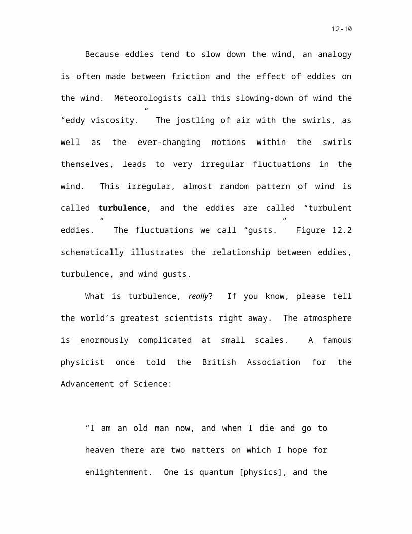
Because eddies tend to slow down the wind, an analogy is often made between

friction and the effect of eddies on the wind. Meteorologists call this slowing-down of

wind the “eddy viscosity.” The jostling of air with the swirls, as well as the ever-

changing motions within the swirls themselves, leads to very irregular fluctuations in the

wind. This irregular, almost random pattern of wind is called turbulence, and the eddies

are called “turbulent eddies.” The fluctuations we call “gusts.” Figure 12.2

schematically illustrates the relationship between eddies, turbulence, and wind gusts.

Eddies are swirls in a fluid, such as air, that interact with the wind and help slow it down in a friction-like way.

12-6

What is turbulence, really? If you know, please tell the world’s greatest scientists

right away. The atmosphere is enormously complicated at small scales. A famous

physicist once told the British Association for the Advancement of Science:

“I am an old man now, and when I die and go to heaven there are two

matters on which I hope for enlightenment. One is quantum [physics],

and the other is the turbulent motion of fluids. And about the former I am

rather optimistic.”

Therefore, you can be content with a definition of turbulence that comes from

experience with aircraft flights: “in-flight bumpiness

due to small-scale changes in the wind.” Box 12.1

explores the fascinating and unsolved problem of

clear-air turbulence.

To summarize what we’ve covered so far: the atmosphere contains wind patterns

at many different scales. At the smaller scales, winds are slowed down and made

irregular—turbulent—by the effect of eddies. This friction-like process is a “brake” on

the natural tendency of the pressure gradient force to push air from high to low pressure

at all scales. And at the tiniest scales, true friction—the rubbing-together of molecules—

does take place and robs the eddies of the energy they steal from the larger-scale wind.

Meteorologist L. F. Richardson, the hero of the next chapter on weather forecasting,

expressed this complicated chain of events in a memorable little rhyme:

Turbulence is the irregular, seemingly random pattern of motion in a fluid such as air. In the context of air travel, it is bumpiness in flight due to these irregular wind patterns on small scales.

12-7

Big whirls have little whirls that feed on their velocity

And little whirls have lesser whirls and so on to viscosity—

in the molecular sense.

An American tour of small-scale winds

From east to west, and generally from large to small, we begin our tour of small-

scale winds in the lower 48 United States (Figure 12.3). Some of these winds are unique

to their locations, but others can be found all across the country and world. Time and

again we will find that our formula PRESSURE GRADIENT + GEOGRAPHY =

SMALL-SCALE WINDS is able to explain the presence, if not all the details, of a

country’s worth of different winds on local scales. We will also find, not surprisingly,

that the change of seasons plays a governing role in the exact nature and role of the wind.

Fasten your seat belts low and tight across your laps, here we go!

The East and South

Back-door cold fronts and cold air damming

We begin at the northeastern extreme of the United States, in New England. At

these higher latitudes, nearby Canada and the north Atlantic Ocean, the air can be cool or

cold in nearly every month of the year. This cold, dense air can, on occasion, build up

and develop enough of a pressure gradient that it slides south of its own accord. The

Appalachian Mountains just to the west help funnel the air. In less than a day the cold air

can slip down the East Coast between the mountains and the coast, sometimes as far

south as Georgia. Upon arrival, cold air likes to stay in place at the surface, particularly

12-8

just east of the high peaks of the southern Appalachians in the Carolinas and Virginia in

winter.

The rapid slip-sliding of cold air south along the East Coast is called a back-door

cold front, particularly in summer. It’s called “back-door” because the front moves

southwestward along the East Coast instead of the more typical southeastward direction.

(Similarly, in basketball a “back-door” basket is one where the player approaches the

basket from the side, not from the front.) The stubborn entrenchment of cold air,

especially in and near the Carolinas and in winter, is called cold air damming. Both of

these phenomena vex weather forecasters because it is so hard to know when the cold air

will plunge south, and when it will dig in its heels and refuse to leave the valleys.

Residents of the East Coast applaud the arrival of a back-door cold front in

summer, because it brings relief in the form of lower dew points and sometimes lower

temperatures. Figure 12.4 is a weather-map example of a fairly typical back-door cold

front; dew points north of the front are 5-10ºF lower than south or west of the front,

which extends across the Virginias and North Carolina.

Cold air damming, on the other hand, can cause transportation nightmares in

winter. As we learned in Chapter 4, freezing rain is likely when warm air falls into a

shallow layer of below-freezing air. Cold air damming is the classic case of shallow cold

air. When warm moist air from the Gulf of Mexico or the Atlantic overruns a case of

cold air damming, a damaging ice storm is a definite possibility. (This may explain why

the title of a research journal article, mistakenly or not, included the phrase “cold air

damning”!)

12-9

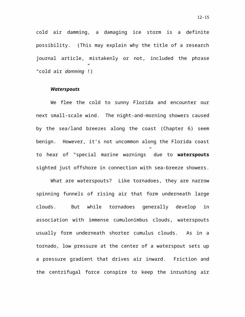
Waterspouts

We flee the cold to sunny Florida and encounter our next small-scale wind. The

night-and-morning showers caused by the sea/land breezes along the coast (Chapter 6)

seem benign. However, it’s not uncommon along the Florida coast to hear of “special

marine warnings” due to waterspouts sighted just offshore in connection with sea-breeze

showers.

What are waterspouts? Like tornadoes, they are narrow spinning funnels of rising

air that form underneath large clouds. But while tornadoes generally develop in

association with immense cumulonimbus clouds, waterspouts usually form underneath

shorter cumulus clouds. As in a tornado, low pressure at the center of a waterspout sets

up a pressure gradient that drives air inward. Friction and the centrifugal force conspire

to keep the inrushing air from collapsing the spout. This air rises and cools, causing

condensation and making the funnel visible. Fair-weather waterspouts are not to be

confused with tornadoes (called “tornadic waterspouts”) that form underneath

cumulonimbus clouds over land and then move over water. Figure 12.5 shows a

waterspout near the Florida Keys as viewed from an airplane; Figure 12.6 is a century-

old photograph of a waterspout witnessed by thousands of vacationers as it churned off

Martha’s Vineyard, Massachusetts.

Even at their most intense, waterspouts are only as strong as weak tornadoes.

This is partly because the wind patterns that help the waterspout spin are limited to near

the surface. In contrast, in Chapter 11 we learned that many tornadoes form inside

thunderstorms that rotate all the way up, from base to anvil. Nevertheless, waterspouts

can cause damage, so we hurry on to the next stop on our tour.

12-10

Microbursts

One particularly nasty type of small-scale wind develops when rain falls from a

thunderstorm on a hot summer afternoon. If the air underneath the thunderstorm is fairly

dry, then the falling rain readily evaporates into it. Evaporation removes heat from the

air, cooling it quickly. This cold, dense air plunges to the surface and “splashes” against

the ground like a bucket of cold water. The cold air then rushes sideways and swirls

upward due to the pressure gradient between the cold air and the warm surroundings (see

Figure 12.7, a photograph of this “splashing”). This wind is a microburst. It is

sometimes also called a “downburst.”

The winds from a microburst can cause as much damage as a small tornado,

flattening trees and power lines. Microbursts that occur near airports are particularly

dangerous. Strong microburst winds from above, below, and sideways buffet aircraft in

just a few seconds. Planes that are landing or taking off can lose airspeed and get pushed

into the ground, causing deadly crashes (Figure 12.8). Microbursts have led to major air

disasters in New York City, Charlotte, New Orleans, and Dallas, killing many hundreds

of people. (Microbursts also occur frequently near Denver. The higher frequency of

thunderstorms in the East and South, combined with heavy airline travel in these regions,

focuses attention in those regions.)

One microburst-related aviation event almost changed U.S. and world history.

On August 1, 1983, Air Force One was ferrying President Ronald Reagan back to

Andrews Air Force Base near Washington, DC. The President and his plane landed on

the dry runway, uneventfully, at 2:04 pm Eastern time. An approaching thunderstorm

then generated a massive microburst that, less than seven minutes later, caused winds

12-11

above 150 mph to blow across that same runway (Figure 12.9)! The microburst even had

an “eye” and a second round of high winds, a little like a mini-hurricane. If President

Reagan’s plane had approached the airport just a few minutes later, a crash would have

been nearly unavoidable.

Spurred by disasters and close calls such as the President’s, the U.S. government

has spent millions of dollars on microburst-detecting equipment at airports. Fewer

microburst-related disasters occur now, thanks to this technology and to extensive pilot

training. Crashes related to microbursts today are usually due to poor decisions by

pilots.

Gravity waves

Have you ever looked up in the sky and seen very straight, parallel lines of clouds

that were there one minute, gone the next? These cloud patterns are all around us. They

occur when the wind is jostled. This jostling can be caused by wind blowing over a

mountain, or by a growing thunderstorm that blocks the wind’s path as if it were a

mountain, or by complicated changes in winds at the jet-stream level. No matter the

cause, the result of this jostling is very similar to dumping a bucket of water in a

swimming pool: waves develop.

These atmospheric waves are known as gravity waves, due to the fact that their

alternating pattern of high and low pressure is maintained with the help of gravity. When

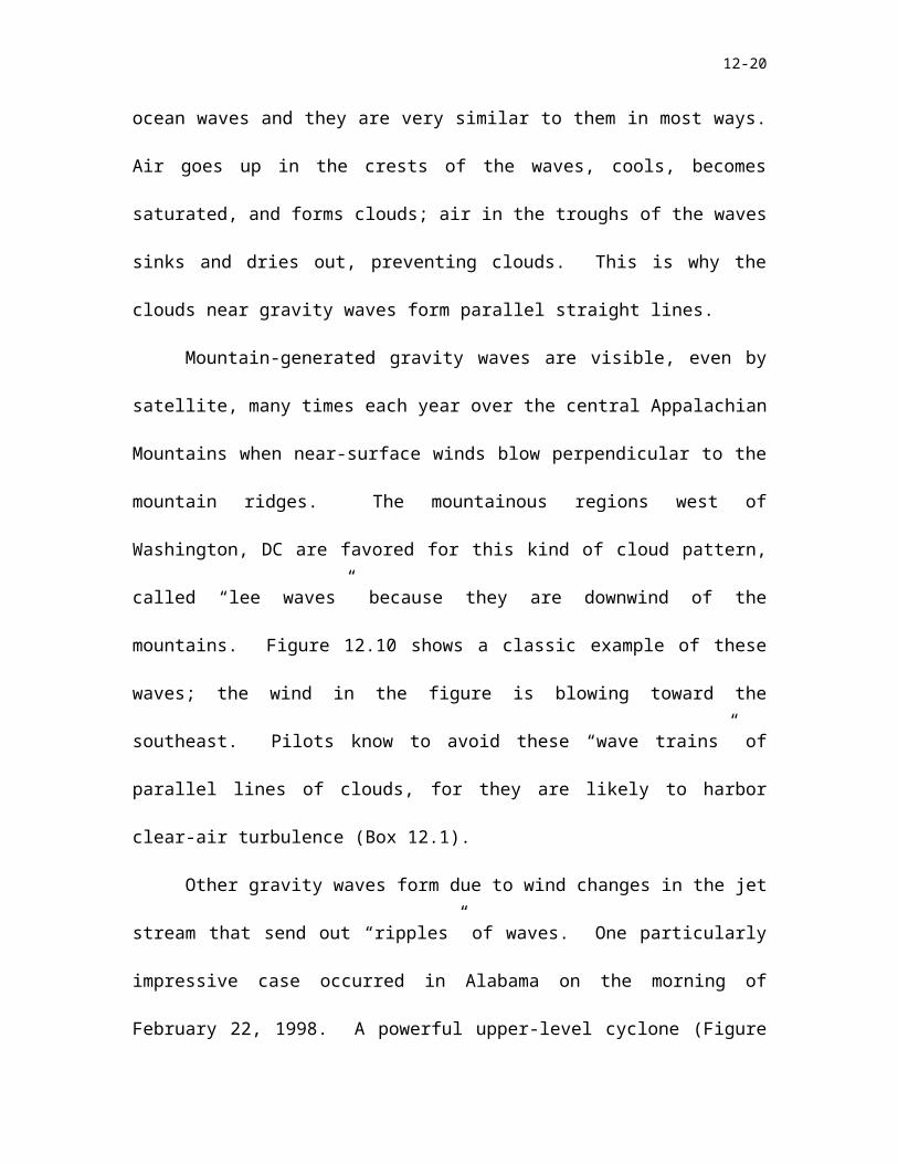
made visible by clouds, gravity waves in the atmosphere look like ocean waves and they

are very similar to them in most ways. Air goes up in the crests of the waves, cools,

becomes saturated, and forms clouds; air in the troughs of the waves sinks and dries out,

preventing clouds. This is why the clouds near gravity waves form parallel straight lines.

12-12

Mountain-generated gravity waves are visible, even by satellite, many times each

year over the central Appalachian Mountains when near-surface winds blow

perpendicular to the mountain ridges. The mountainous regions west of Washington, DC

are favored for this kind of cloud pattern, called “lee waves” because they are downwind

of the mountains. Figure 12.10 shows a classic example of these waves; the wind in the

figure is blowing toward the southeast. Pilots know to avoid these “wave trains” of

parallel lines of clouds, for they are likely to harbor clear-air turbulence (Box 12.1).

Other gravity waves form due to wind changes in the jet stream that send out

“ripples” of waves. One particularly impressive case occurred in Alabama on the

morning of February 22, 1998. A powerful upper-level cyclone (Figure 12.11)

unexpectedly triggered gravity wave ripples that moved northward across the entire state

of Alabama (a distance of over 250 miles) in only three hours. In downtown

Birmingham (Figure 12.12) the surface pressure dropped 10 millibars in just 17 minutes.

The corresponding tight pressure gradient caused winds over 22 m/s (51 mph). Houses

and trees exposed on the sides of small mountains in the Birmingham area, unsheltered

by the effects of friction, experienced winds around 60 mph; roof and tree damage was

extensive. Yet no thunderstorm was involved; the winds were all part of the waves

generated by the sloshing of the jet stream high above! The local weather forecasters

were taken completely by surprise. We learn in the next chapter that some of these same

forecasters made a brave, and accurate, forecast of a record snowfall in Alabama just a

few years before. The forecasting of small-scale winds can be extremely difficult, harder

than the most complicated large-scale weather event.

12-13

Gravity waves, because of the wide variety of ways in which they are triggered,

can be observed in all parts of the country. Figure 12.13 shows a classic satellite image

of a series of gravity waves ahead of a cold front in southern Texas.

The Midwest

West of the Appalachians, we encounter the Midwest. In Chapter 10 we learned

a lot about the localized windstorm that helped sink the Edmund Fitzgerald. Now it’s

time to explore the unique features of Midwestern winds, most of which are related to the

presence of the immense Great Lakes.

Lake-effect snow revisited

The Great Lakes dominate the weather of the Midwest, especially the upper

Midwest. In winter, as we have seen, cold cP air blowing across long enough stretches

of open, warmer Great Lakes water leads to lake-effect snow (Figure 12.14).

Geography is everything to lake-effect snow. The transfer of energy and water

vapor to the air is dependent on the lakes. The shape of the lake determines the “fetch”

or distance the wind blows over the lake. Finally, the wind slows down or “converges”

when it reaches shore due to increased turbulent friction. This helps the snow intensify

just onshore, especially if there are hills near the shore to give a little extra lift to the air.

All of these factors combine to create “lake-effect snow belts” that are narrow but

concentrated. The amount of snow in a typical year can vary by a factor of two or more

in the space of just a few miles!

While widespread lake-effect precipitation is unique to the upper Midwest, it is

not unique to winter. Lake-effect rain, lake-effect sleet, lake-effect drizzle, or lake-effect

12-14

cloudiness can all be observed in the upper Midwest whenever the air blowing over the

Great Lakes is significantly cooler than the lake waters. This is most common in

autumn.

Lake breezes

During warm summertime days, the Great Lakes are usually colder than their

surrounding coastlines. These lakes are so large that local wind circulations develop due

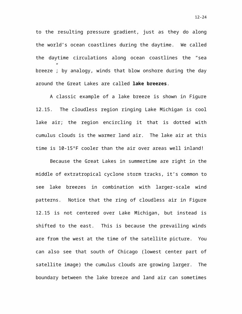
to the resulting pressure gradient, just as they do along the world’s ocean coastlines

during the daytime. We called the daytime circulations along ocean coastlines the “sea

breeze”; by analogy, winds that blow onshore during the day around the Great Lakes are

called lake breezes.

A classic example of a lake breeze is shown in Figure 12.15. The cloudless

region ringing Lake Michigan is cool lake air; the region encircling it that is dotted with

cumulus clouds is the warmer land air. The lake air at this time is 10-15ºF cooler than

the air over areas well inland!

Because the Great Lakes in summertime are right in the middle of extratropical

cyclone storm tracks, it’s common to see lake breezes in combination with larger-scale

wind patterns. Notice that the ring of cloudless air in Figure 12.15 is not centered over

Lake Michigan, but instead is shifted to the east. This is because the prevailing winds are

from the west at the time of the satellite picture. You can also see that south of Chicago

(lowest center part of satellite image) the cumulus clouds are growing larger. The

boundary between the lake breeze and land air can sometimes be a focal point for

thunderstorm development, just like a small-scale cold front.

12-15

River fog

It’s only fair to include one local weather phenomenon due to the lack of small-

scale winds interacting with geography. When a clear, cool autumn anticyclone passes

over the Midwest, its secluded river valleys become calm and even cooler than the

surrounding regions. Because the rivers are a constant moisture source, the calm air is

easily cooled to its dew point. Fog forms in the early morning over the river and along

its banks. On some occasions, as in Figure 12.16, this river fog outlines the river valleys

of the Midwest as clearly as a fine-point highlighter pen. This remarkable sight

disappears by late morning in most cases, as the returning sun heats the ground, creates

pressure gradients, and stirs up the air.

To read about how humans use turbulent friction to advantage in the snowy

Midwest and the dusty Great Plains, see Box 12.2 on snow fences and shelterbelts.

Derechos

At the opposite extreme from the calm of river fog is the derecho. A derecho

(pronounced duh-RAY-sho, the Spanish word for “straight” or “right”) is an hours-long

windstorm associated with a line of severe thunderstorms. It is due to straight-line

winds, not the spinning winds of a tornado; hence, its name.

The extreme winds of a derecho—up to 150 mph in the worst cases—come about

in the following way. Derechos are often associated with stationary fronts in mid-

summer. The fronts aren’t moving, but they are boundaries of different air masses with

different temperatures. Above these fronts lie relatively strong jet streams (see Chapters

7 and 9). A line of thunderstorms that forms in the vicinity of the stationary front can,

12-16

via its cold downdrafts, drag down the high-speed air from above. This can cause the

high winds of a derecho.

These high winds near the surface bulge the line of thunderstorms outward,

causing it to bend or “bow” in the direction of the wind. This is called a “bow echo”

when it is seen on weather radar. Because the thunderstorms are pushed rapidly by the

jet stream, they cover lots of territory—often hundreds of miles. Derechos leave

significant property damage, and even entire forests flattened, in their wake.

Figure 12.17 shows a radar image of a classic derecho that caused three deaths

and 70 injuries and left 600,000 people without power in Michigan on May 31, 1998.

Notice the characteristic bowed-out pattern of the squall line on radar. This line of

storms moved at a forward speed of 70 mph, carving a path of non-tornadic destruction

from South Dakota to New York state.

Wake lows

The passage of a dying thunderstorm can sometimes be the cause for high winds

in summer. Behind a few storms, a small region of very low pressure called a wake low

develops. It’s called a “wake low” because it forms behind the path of, or in the wake of,

the thunderstorm. The pressure gradient near a wake low is very strong—a large change

in pressure over a short distance during a relatively short time. Therefore, the air blows

straight from high to low pressure; the Coriolis force cannot balance the pressure

gradient force. Since the storm is passing, this creates the unusual situation of high

winds blowing away from, not into, the thunderstorm—and the thunderstorm is

weakening and leaving your vicinity!

12-17

On June 30, 1993, a thunderstorm on the northern fringe of the storms causing the

1993 Upper Mississippi floods triggered a wake low that passed through Madison,

Wisconsin. Figure 12.18 shows the remarkable change in pressure that occurred in

Madison during a few short hours early in the morning of the 30 th: a drop of 16 millibars

in less than 2 hours! Sleepy residents awoke to strong and sustained winds of up to 50

mph, even though the thunderstorm had already passed through the city and was

diminishing.1 This is a reminder that strong winds are related to strong pressure

gradients, no matter what the situation is.

The Great Plains

The Great Plains are nearly flat, tilt gradually upward from east to west, and at

their western edge are close to the high mountains of the Front Range of the Rocky

Mountains. These facts help explain every small-scale wind that follows!

Nocturnal low-level jet

We learned in Chapter 10 that the lee of the Rocky Mountains is a preferred place

for low-pressure systems to form. Because winds around a low blow counterclockwise

in the Northern Hemisphere, a low in eastern Colorado or the Texas Panhandle causes

south winds ahead of the low over the Great Plains. During the spring and summer,

these winds bring moist air from the Gulf of Mexico as far north as Canada. Like a lane

at the bowling alley, the flat Plains offer little resistance to the flow of air northward.

1 To see one of your author’s impressions of this particular windstorm in poetic form, go to http://www.valpo.edu/english/vpr/v2n1.html

12-18

During the day, winds in the lowest kilometer of the atmosphere are slowed down

by turbulence. The heating of the sun sets turbulent eddies in motion that, in effect, hold

back the southerly winds like a rough surface.

At sunset, however, the turbulent eddies die down. Without the effect of eddy

viscosity, the winds above the surface speed up, skidding along like a bowling ball on a

heavily waxed lane. With help from the sloping Plains, these winds can rev up to 20

knots or more, blowing to the north. Figure 12.19a, b, and c illustrate how this jet works

and what it looks like on Doppler radar.

This nighttime wind maximum is called the nocturnal low-level jet, making the

analogy with the much higher-speed jet streams near the tropopause. This is a small-

scale wind in the vertical, because it is confined to a narrow region just a few hundred

meters above the ground. This wind plays an important role in thunderstorm growth

over the Great Plains as far north as the Dakotas.

To give one example, you may have noticed that the stormchasers in the Great

Plains often film their exciting videos near sunset. This is rather late in the day for

thunderstorms in other parts of the nation. Furthermore, the storms they chase can

intensify after dark, even as late as midnight. How can this be, if daytime heating fuels

thunderstorms? One answer is that the nocturnal low-level jet pumps more and more

warm, moist air into mesoscale convective complexes (Chapter 11) long after sunset,

prolonging the lifetimes of these giant thunderstorm systems.

At dawn, the rising sun stirs up the surface air again, the winds above the surface

are slowed by turbulent eddies, and the low-level jet disappears—until the next evening!

12-19

Dryline

Our next Great Plains wind also helps trigger thunderstorms, but it is a dry low-

level wind. In late springtime, dry cT air (Chapter 9) from the plateaus of Mexico is

drawn northeastward into the Texas Panhandle ahead of extratropical cyclones in the lee

of the Rockies. While the difference in temperature may be small between the cT air and

the warm mT air covering eastern Texas, the clash in dew points is literally breathtaking:

10ºF or more over just a few miles. This small-scale frontal zone defined by moisture,

not temperature, is known as the dryline. Figure 12.20 illustrates the analysis of a

dryline on a weather map.

The dryline helps provide a focus for thunderstorm activity over Texas and

Oklahoma in late spring, to the delight of stormchasers. Air converges and lifts at the

dryline, leading to thunderstorms just as with a cold front. In a region that averages only

about ten inches of rain each year, these thunderstorms are a crucial part of the annual

water supply. Therefore, the dry parching wind behind the dryline actually plays a key

role in the agriculture of the semiarid regions of central and west Texas.

Blue norther

We learned that the nocturnal low-level jet can blow all the way north from Texas

into Canada because of the lack of any mountain range to impede its travels. In winter,

Canada returns this favor. The Plains offer little resistance to cold air pushing south in

winter. The Rocky Mountains help channel southward pushes of cP air even more

effectively than the Appalachians do for back-door cold fronts. As a result, cold fronts

can sometimes zoom across the 1500 miles of the western Plains, from the Dakotas to

Texas, in only a couple of days.

12-20

As the front enters Texas, the temperature clash at the fronts can be extraordinary.

Temperatures can drop tens of degrees in only a few hours. However, the air on either

side of the front is extremely dry, having originated either in the dry high hills of the

Southwest, or else bone-dry Canada. Therefore, the front is accompanied by clear blue

skies. The only sign of changing weather is when the mercury in the thermometer drops

so fast you can see it move! This is why the fierce north wind behind a fast-racing cold

front in west Texas is known as a blue norther.

Blue northers can be killers. Farmers or hunters unprepared for their arrival can

freeze to death, particularly if the initial clear-sky front is followed by snow. Their high

winds can, in times of drought, also lead to dust storms. Box 12.3 examines dust storms

and the infamous “Dust Bowl” of the 1930s in more detail.

Chinook

On the western edge of the Great Plains, flatlands meet mountains. When air

moves down these mountain slopes, it goes down in a hurry. The peaks of the Rockies

are 10,000 feet or higher; the Colorado plains are a mile high. The highest Black Hills of

western South Dakota are over 7,000 feet tall; the nearby towns and cities are at about

3,000 feet of elevation. We learned in Chapter 2 that when air is brought downward in

the atmosphere, adiabatic compression leads to warming and drying-out of the air. A

dry, warm wind results whenever the large-scale pressure gradient forces air down the

slopes of the Rockies, or the Black Hills of western South Dakota, onto the plains. Plains

residents call this dry, warm wind a chinook.

The chinook’s nickname of “snow eater” arises because a chinook quickly warms

a location above freezing while dropping its relative humidity into the single digits.

12-21

Snow is able to melt and evaporate rapidly under these windy conditions. Not far from

Rapid City, SD on January 22, 1943, a chinook rocketed the temperature up from -4ºF to

45ºF in only two minutes, a world record!

On the Plains, these extreme changes are mostly a curiosity, significant only for

farmers and the comparatively few residents of the area. We will see that when the same

type of wind occurs on the heavily populated West Coast, it is as big a threat to life and

property as El Niño or earthquakes.

The West

The Western United States enjoys the richest array of small-scale winds because

its geography is the most varied, from tall peaks to flat deserts. Many of the local wind

patterns we have already studied, such as microbursts, gravity waves and cold air

damming, are frequently observed in the mountain West as well. Other winds are unique

to the complex geography of the West. Once again, we can explain their existence

through simple application of pressure gradient ideas and attention to the shape and

character of the nearby geography.

Mountain/valley breezes and windstorms

We’ve already discussed how temperature differences between ocean and

coastline, or a Great Lake and its shores, can lead to pressure gradients that drive local

wind circulations. The same thing can happen along the slopes of high mountains such

12-22

as the Rockies. These small-scale winds are called mountain and valley breezes, and

closely resemble the ocean and land breezes of Chapter 6.

Figure 12.21 is a schematic of how these breezes develop. During the day, the

thin air above the high mountainsides warms quickly. The warm air rises and creates

local low pressure along the slopes. Air from the lower valleys moves in to replace it,

creating an upslope breeze that becomes strongest around noon. This is the valley

breeze.

At night, the high mountain slopes cool very quickly. This cold, dense air forms

a local high-pressure area. The pressure gradient drives a gentle breeze down the slope

into the valley that is strongest just before sunrise. This is the mountain breeze.

Mountain and valley breezes are usually just a few miles per hour. Even so, they

can have a profound impact on local weather and climate. Figure 12.22 shows an

example from northern Utah in which cold air sinking into a valley in winter causes a

reverse treeline, below which it is too cold for trees to survive!

In mountainous regions with large plateaus with steep sides and lots of snow on

the ground, the cool mountain breeze is anything but gentle. In some cases wind gusts

can exceed 100 mph! These more violent relatives of mountain breezes are called

katabatic winds. They occur in the West in places like Colorado and the Columbia

River valley. Their violence is due to the strong pressure gradient built up by the chilling

of air over the high snowy plateau, and the steep slopes that allow the wind to rush

downhill quickly.

Still other mountain winds affect the West. Any time there is a strong pressure

gradient across the mountains the wind tries to find a place to break through the barrier

12-23

of rock. Low points in the mountains, called “gaps” or “passes,” become wind tunnels in

these cases. The gap winds that develop can easily exceed 100 mph in the strongest

cases.

In Boulder, Colorado just northwest of Denver, downslope winds associated with

mountain gravity waves can cause particularly ferocious Boulder windstorms. Winds

well over 100 mph have been observed in some cases! Figure 12.23 depicts the winds

from a comparatively mild Boulder windstorm. These windstorms cause considerable

property damage; in areas such as Boulder, building codes have had to be changed to

reduce the amount of damage.

Dust devils

A much more benign wind blows along the sands of the desert Southwest. There,

intense daytime heating helps spin up thin rotating columns of air called dust devils

(Figure 12.24). Unlike its cousins the tornado and the waterspout, the dust devil appears

to be a creature created solely by solar heating. The hot sun of Arizona bakes the ground

until the surface air becomes unstable and rises, creating a local low-pressure center

usually only a few meters across and 100 meters tall. As the little vortex begins to spin,

dust and sand is drawn into the circulation and a dust devil is born. It usually lasts only a

few minutes.

Unlike waterspouts and tornadoes, dust devils do not require any clouds, showers,

or thunderstorms above them; they form under clear skies in a hot sun. Like waterspouts,

the winds in a dust devil are much less than in tornadoes, and damage from them is rare.

Lenticular clouds

12-24

As we approach the mountains of the Coastal Range, we encounter another small-

scale wind and cloud feature that combines the beauty of the dust devil with the beast of

a Boulder windstorm. It is called a lenticular cloud (Figure 12.25).

The name “lenticular” means “lens-shaped.” These clouds hang over

mountainous regions for hours, moving little if any. To modern eyes, lenticular clouds

resemble the hovering motherships of space alien movies. In fact, the first modern

“sighting” of a UFO occurred near Mount Rainier, Washington, and was probably a type

of lenticular cloud.

What does a lenticular cloud have to do with small-scale winds? Everything.

When winds blow across high mountain ranges in certain circumstances, vigorous gravity

waves develop downwind of the mountains. Air rising on the crest of the wave just past

the mountain becomes saturated, forming the lenticular cloud. Because the wind and the

mountain anchor the wave crest in the same place, the cloud is stationary—just as a

swirling river eddy downstream from a rock stays in the same spot. The swirling pattern

of winds around and over the mountain sculpts the lenticular cloud into unique and ever-

changing shapes.

The beauty of the lenticular cloud sounds a warning alarm to pilots. The wind

circulations in and near lenticular clouds are extremely turbulent (Figure 12.26), despite

the seemingly calm, smooth appearance of the cloud. All aviators should avoid these

clouds.

Santa Ana winds

Upon our westward descent over the coastal mountains of California, we discover

yet another downslope wind. This wind, the Santa Ana wind, combines the

12-25

characteristics of its close kin the chinook with the damage potential of a Boulder

windstorm.

The Santa Ana wind occurs when the large-scale pressure gradient, in

combination with friction, forces already dry air from the mountainous West down the

Coast Range in northern California, or the San Gabriel Mountains in southern California.

This happens most often in the months of autumn. As with the chinook, the temperature

increases and the humidity plummets in a Santa Ana.

There are a few key differences between chinooks and Santa Anas, however.

There is no snow for the Santa Ana to “eat” in fall in California. The trees and grasses of

California are naturally dry in autumn. Also, tens of millions more people live in the

way of the Santa Ana. As a result, the Santa Ana wind turns some of America’s largest

metropolitan areas into a bone-dry, roasting tinderbox. One spark, cigarette butt, or

lightning strike later, regions affected by the Santa Ana wind become huge roaring fires.

On October 20, 1991, a Santa Ana wind with speeds above 20 mph dropped the

relative humidity in the Oakland, California vicinity to less than 10% for an entire day.

The remains of a brush fire flared up, and the inferno was on. When the fire (Figure

12.27) was finally extinguished, 25 people were dead, over 2,000 buildings were

destroyed, and damage was assessed in the billions of dollars.

A similar Santa Ana wind-related fire four years after the Oakland conflagration

burned Point Reyes National Seashore just north of San Francisco. Near the coast,

temperatures were in the 80s, but dew points were only in the teens. The smoke from the

raging fire showed up on satellite photographs for 1,000 miles out to sea (Figure 12.28)!

12-26

The Catalina eddy

We conclude our tour in the cool waters off the coast of Southern California, a

continent away from where we began. Although by reputation the Los Angeles area is

always sunny, in fact the cool ocean current just offshore helps promote low clouds and

fog off the coast. Sometimes in spring and summer, the stratus and fog invade onshore,

staying until mid-afternoon and interfering with air travel (but also clearing out the ever-

present pollution). Why does the fog roll onshore on some days, but not others? The

Catalina eddy.

The Catalina eddy is a small-scale swirl of air that develops just off the Los

Angeles coastline near Santa Catalina Island. It’s bigger than the turbulent eddies we’ve

talked about, usually tens of kilometers across, but much smaller than an extratropical

cyclone (Figure 12.29). It develops when there is a large-scale pressure gradient in the

region. The resulting winds interact with the coastal islands, the high mountains just

inland, and the shape of the coastline, and develop into a small spiraling low. Just east of

the swirl, its southerly winds blow over the cool ocean waters and then inland over Los

Angeles. The water vapor in the cool and moist air condenses. Fog rolls into the City of

Angels!

The Catalina eddy is not a killer like the Santa Ana wind. Just the same, weather

forecasters in southern California must know when to expect this small-scale wind

pattern and anticipate its effects on one of the world’s great cities.

Putting it all together

Let’s step back and survey the small-scale winds of the lower 48 United States

(Figure 12.30). Geography is destiny for these winds. The Hoosiers of Indiana need

12-27

never fear a Santa Ana, and residents of Olympia, Washington will probably never suffer

a derecho or a wake low.

Our tour was not all-inclusive geographically, however. The high craggy peaks

of Rockies actually cause more gravity waves than the shorter, smoother Appalachians.

But it’s possible to see lenticular clouds over the little knob hills of western Kentucky!

The moral: small-scale winds and their visible signatures are all around us, occurring at

any time and place for which the combination of pressure gradient and geography is just

right.

This moral means that we cannot stop looking for small-scale winds at the

borders of the United States. Indeed, they are everywhere. In many cases, though, these

winds are simply variants on the kinds of winds observed in the U.S. Figure 12.31

identifies a few of these international small-scale winds, relating each to its closest

American cousin.

Summary

Winds occur on every scale imaginable, from large to small. Small, quick winds

are driven primarily by the pressure gradient force and are slowed down by the effects of

“friction.” The main type of friction in a fluid such as the atmosphere is actually

turbulence due to swirling eddies of different sizes. These eddies are stirred up by the

sun, by wind blowing around obstacles, and by the atmosphere itself. This causes the

characteristic gustiness of winds that you see around you nearly every day.

An amazing variety of small-scale winds exist in the United States. Some winds

are gentle, such as those that promote river fog in the Midwest, slide mountain breezes

down the sides of the Rockies, or ooze fog into the Los Angeles basin. Other winds are

12-28

violent, dropping out of thunderstorms or blowing along the Front Range of the Colorado

Rockies. A few are deceptive, hiding a commotion of turbulence inside a smoothly

sculpted cloud. There are dry winds that eat snow and cause fires, and other dry winds

that promote rainfall. And there are the ubiquitous rippling gravity waves that draw lines

in clouds and, on rare occasions, spark windstorms. Small-scale winds are everywhere.

These kinds of winds are not limited to the United States. A dazzling array of

small-scale winds exists worldwide. For all of their diversity, however, small-scale

winds on our planet can generally be explained as the interaction between a pressure

gradient and geographic features such as mountains, plains, lakes, or coastlines. The

colorful, unique names and rich histories of these local winds disguise the fact that they

are all “brothers under the skin.”

12-29

Terminology

You should understand all of the following terms. Use the glossary and this Chapter to

improve your understanding of these terms.

Back-door cold front

Blue norther

Boulder windstorms

Catalina eddy

Chinook

Cold air damming

Derechos

Dryline

Dust devils

Dust storms

Eddies

Gap winds

Gravity waves

Katabatic winds

Lake breezes

Lake-effect snow

Lenticular clouds

Mesoscale

Microbursts

Microscale

Mountain breezes

Nocturnal low-level jet

Planetary-scale

River fog

Santa Ana winds

Synoptic-scale

Turbulence

Valley breezes

Viscosity

Wake lows

Waterspouts

12-30

Review Questions

1. A tiny swirl in the bathtub can look a lot like an extratropical cyclone. Using facts

from this chapter, explain why they aren’t the same.

2. Why do meteorologists link turbulence with friction, when in fact there aren’t any

rough surfaces rubbing together in the atmosphere?

3. Go to your kitchen or bathroom and make three different sizes of eddies. What

causes them, how big are they, and how long do they last?

4. Why are waterspouts more common on the East and Gulf Coasts than on the West

Coast?

5. On a U.S. map that includes elevations, find the highest mountain peaks in the entire

eastern United States. Does their location surprise you? How does their location

affect cold air damming events?

6. Why is the low-level jet “nocturnal,” like an owl or an opossum?

7. Would mountain or valley breezes be more intense on the northern or the southern

slopes of a mountain? Why would there be a difference?

8. Based on your understanding of gap winds, explain why the streets of skyscraper-

filled Manhattan can be so windy on a day when the winds in the suburbs around

New York are light-to-moderate.

9. A real estate agent tries to sell you a house in Colorado that’s near the bottom of a

valley, ringed by tall mountains. The view is gorgeous. What meteorological

advantages and disadvantages are there to purchasing a house in this location? How

would your heating and cooling costs be different if the house was up near the

mountain peaks?

12-31

10. It’s a hot sunny day in Dallas, Texas. A low is approaching from the west, however.

What different kinds of small-scale winds could lead to turbulence for a plane taking

off and ascending, or descending and landing, near Dallas?

11. Why are windmills and wind turbines placed on tall towers, where their moving parts

are annoyingly hard to get to?

12. An old folklore saying goes, “The winds of the daytime wrestle and fight/Longer and

stronger than those of the night.” Based on what you’ve learned about turbulent

eddies, explain why this is usually true. What Great Plains wind contradicts this age-

old wisdom?

13. The planet Mars has very high mountains and flat plains. It’s very dry (few clouds,

no thunderstorms) and dusty. Its axis tilts about the same as Earth’s, so that Mars’s

tropics receive a lot of sunshine all year long. Based solely on this information and

facts found in this chapter, what kinds of small-scale winds would you expect to find

on Mars?

14. It’s the week before your wedding. You’re in your seventh-story apartment watching

television with your fiancé(e). Suddenly, the local TV weatherman comes on, shows

the radar, and points out a “bow echo” approaching quickly. What kind of small-

scale wind is coming? What should you do immediately? (This is a true story!)

15. A neighbor says, “I don’t care about all those other watches and warnings, the only

thing that scares me is a tornado.” Tell the neighbor what other kinds of small-scale

winds can cause damage almost as severe as a tornado, and why.

Web Activities

Web activities related to subjects in the book are marked with superscript . Activities:

12-32

1. There exists a video simulation of the Charlotte, NC USAir crash in 1994. Mike

Smith, CEO of WeatherData, Inc. of Wichita, KS has a copy because he testified in the

trials that ensued. In 1999 I also found a copy of it as a movie file on the Web, but the

video was later removed from the Web and I don’t think I saved a copy.

This simulation would be wonderful to have as a movie on the Web. It shows, from the

perspective of someone in the cockpit, the last couple of minutes of the USAir flight,

complete with read transcriptions of the pilots’ communications from the flight data

recorder and the tower tapes. You see the plane getting bounced around by the

microburst winds. At the end, you see the plane pulling up, trying to do a go-around, and

then crashing. It’s stunning. The pilots survived (many passengers did not), but it was

definitely pilot error and the pilots weren’t even fired by USAir—so I wouldn’t feel too

horrible about using it for educational purposes. Something good should come of the

waste. The question is whether or not the video can be obtained and used for our

purposes.

2. The GOES Gallery found at http://cimss.ssec.wisc.edu/goes/misc/ has an excellent

loop of a gravity wave event on March 19, 1998 that occurred near Brownsville, TX..

3. At the very end of the 1996 National Geographic TV special “Cyclone!,” a snippet of

home video is shown of a dust devil (I think in the northeast U.S.) that is composed

totally of hay, not dust. It is an ethereal, playful sight; just say “hay-nado” to

12-33

meteorologists and they instantly know what you’re talking about. It would be nice to

have that video on our Web site to illustrate, again, that these small-scale winds happen

whenever the conditions are right. (No one told the hay-nado it couldn’t happen because

it wasn’t over Arizona sands!)

4. The international winds are not given as much attention here as in some other texts. A

way to remedy this would be to create a Java-type Web page with a clickable world map.

The student could click on the name of a wind, say, “foehn,” and hear it pronounced

correctly. Then the student could click on the word “details” beneath the name of the

wind and read/hear more about where and when this wind happens, any interesting

details about it, etc. Would Tom like to do this?

12-34

Box 12.1 Clear-Air Turbulence

Airplanes and turbulence don’t mix. Commercial and especially private aircraft

are roughly the same size as large turbulent eddies high up in the atmosphere. This

means that planes travel from one bump to another very quickly. The result can be in-

flight chaos. One airline pilot in the 1970s recalled from a particularly severe encounter

with turbulence:

“I felt as… one might expect to encounter sitting on the end of a huge tuning fork

that had been struck violently. Not an instrument on any panel was readable to their full

scale but appeared as white blurs… Briefcases, manuals, ashtrays, suitcases, pencils,

cigarettes, flashlights flying about like unguided missiles.”

For this reason, pilots avoid regions of turbulence. They know to avoid the parallel lines

of clouds near mountains, lenticular clouds, and the rainy or dusty swirls of microbursts.

However, nature doesn’t always provide a visual indicator for turbulence.

Sometimes, in nearly clear skies high up at cruising altitude, planes will suddenly

encounter the same sort of jarring bumpiness. This is called clear-air turbulence,

abbreviated “CAT” for short. It is one of a pilot’s worst nightmares.

What is clear-air turbulence? One of the main theories is that wind shear—the

change of wind as you go up, which we discussed in Chapter 8—self-develops its own

gravity waves. These waves then rapidly break, like ocean waves on a beach. Waves

35

breaking on a beach generate a lot of foam; the “foam” of a breaking atmospheric gravity

wave is turbulence.

What does CAT look like? By definition, you can’t see clear-air turbulence.

Under the right conditions, however, clouds can form and reveal the process outlined

above. A beautiful example is shown in the figure below.

(Photo Copyright ©1998 by Kay Ekwall, KaRa Productions,

404 N. Mt. Shasta Blvd., Ste.111 Mount Shasta, CA 96067; 1-888-926-1997.

http://www.shastahome.com/kee/waves.htm We’ll have to pay; the watermark will not be

on the final version, obviously.)

Looking left to right, you can see crests of the waves in different stages of breaking. On

the left, the wave crest is just beginning to turn over. At right, it’s a foamy mess. This

36

process is happening all the time in the atmosphere; only rarely do clouds or a high

mountain warn of its presence.

An airplane’s encounter with CAT doesn’t just make for a good story; it is a

destroyer and even a killer on occasion. In December 1992 CAT damaged the cargo jet

below while it was cruising at 31,000 feet over the Colorado Rockies. The plane

survived, minus an engine and twelve feet of the leading edge of its wing (see figure).

(From http://www.rap.ucar.edu/research/turbulence/forecasting.html )

Commercial passenger aircraft clashes with CAT hurt people as well as planes.

On December 28, 1997, a United Airlines 747 jet carrying 393 people to Honolulu from

near Tokyo hit heavy turbulence over the Pacific Ocean. Passengers who happened to be

wearing their seat belts at the time described floating “like we were in an elevator falling

down,” according to the Associated Press. Those not wearing seat belts left dents where

their heads crashed into the ceiling. One woman was killed due to severe head trauma

and at least 102 other people were injured, some of them seriously.

Fortunately, clear-air turbulence this severe doesn’t happen very often. Only

about 1% of every 100 miles of flight will experience severe CAT such as encountered

by the United flight over the Pacific, in which vertical accelerations exceed gravity.

Even when it does happen, CAT persists for only a few minutes in most cases.

37

A phenomenon as silent, invisible, small, and fleeting as clear-air turbulence is a

major challenge for weather forecasters. Tried-and-true rules of thumb exist to steer

airplanes around likely areas of wind shear, such as jet streams. The rules aren’t precise

enough, however. Even today, airplanes fly into unforecast CAT on a daily basis.

Progress toward understanding this special brand of turbulence has been slow—just as

slow as for every other type of turbulence.

Now you know why the airlines tell you to keep your seat belt fastened at all

times!

38

Box 12.2 Using Turbulence to Advantage: Snow Fences and

Windbreaks

On the Great Plains and in the nation’s snow belts, wind can be an enemy. Snow

or dust picked up by the wind can reduce visibility, cover roads, and shut down normal

life for days on end. Unfortunately, there is no “off” switch on the winds. However,

there is a “slow motion button”: the effect of turbulent eddies. This is the concept behind

two human creations, the snow fence and the windbreak.

The presence of obstacles such as fences and trees slows down the wind by

causing turbulent eddies to develop. The wind is broken up into a swirl of eddies and its

overall speed is reduced. This is why a wooded, fenced-in suburb is generally much less

windy than an open field or shoreline. Snow fences use this concept to keep snow from

blowing across land and roadways.

The idea behind a snow fence is, to amend a famous line from the baseball movie

“Field of Dreams”: if you build it, the snow will come—and stay. Snow flying on high

winds past a snow fence will, instead of blowing straight downwind, get caught up in the

turbulent eddies the fence creates. Some of the snow will slow down just past the fence

and drop to the ground. As more and more snow collects behind the snow fence, it

presents an even larger obstacle to the wind. By the time the wind subsides, a large pile

of snow resides behind the snow fence. If the fence is located upwind of a road or a

farm, this is snow that didn’t drift over the asphalt or bury the barn. In addition, in cold

arid regions such as the Dakotas this snow is a moisture source and a blanket, keeping the

ground from becoming frozen too deeply in winter.

39

The same idea holds for windbreaks (see figure) on the dusty Great Plains.

[Photo by USDA-SCS, from: http://www.libfind.unl.edu/nac/pubs/ec/ec1767/]

Blowing dust in spring can be a great hazard to transportation; it is also the precious

topsoil of the farmers, leaving the area. To prevent this, lines or belts of trees called

“windbreaks” or “shelterbelts” have been planted from place to place across the Plains.

The wind blowing past these windbreaks is chopped up into slower turbulent eddies.

Windbreaks function like the “speed bumps” used in shopping center parking lots to keep

cars from going too fast. They keep the winds from roaring across the hundreds of miles

of flat land and lifting freshly plowed soil into the air.

40

Both snow fences and windbreaks make effective use of turbulent eddies. Yet

they come at a (modest) price. In cities, someone has to put up the snow fences in fall

and take them down in spring. In the Plains, someone had to plant the trees on land that

otherwise would have been used for growing crops. The temptation lurks to take down

the fence and cut down the trees. This is penny-wise, pound-foolish thinking that ignores

the basics of small-scale winds. For an example of what can happen when all the trees

are cut down, all the soil is plowed, and the winds blow hard, long, and dry, read Box

12.3 on the “Dust Bowl.”

41

Box 12.3 Dust Storms and the “Dust Bowl”

Dust storms are to dust devils what a mesoscale convective complex (Chapter 11)

is to a thunderstorm: a scaled-up version that has its own unique look. Below is a

photograph of an approaching dust storm.

(Photo by: David Smalley, dave@sleet.plh.af.mil, 781-377-3033 Found at:

http://www.atmo.ttu.edu/dustwall.html )

Meteorologist David Smalley took this picture from the roof of the Business

Administration building on the campus of Texas Tech University in Lubbock, Texas on

October 2, 1983. The thousand-foot-tall dust storm in the distance, powered by winds

42

gusting out of a thunderstorm, reached his location just one minute after the picture was

taken. The pressure jumped 4.4 mb in the next half hour—proof that this wind, like all

the others we study in this chapter, is driven by strong pressure gradients.

Dust storms are not uncommon in the far western Great Plains of the Texas and

Oklahoma Panhandles. As we learned in Chapter 10, extratropical cyclones are born in

the Panhandles, causing windy conditions. Dryline thunderstorms can kick off dust

storms with microbursts. And blue northers can usher in dust on their leading edges as

they race southward from Canada. A pressure gradient, plus dry ground, is all that is

needed. That, plus overly aggressive farming practices, can even lead to a “Dust Bowl.”

In the early decades of the 20th century, American farmers moved into this region

to turn the Plains into an agricultural paradise. The farmers came from the East and the

South. However, those regions typically receive double, triple, or even quadruple the

annual rainfall of the Panhandles. Furthermore, typical wind speeds in the East and

South are lighter than in the high Plains.

Every available piece of soil in the Panhandles was developed for agriculture,

first by horse and plow and later by tractor. Farming practices did not take into account

the precipitation and wind conditions of the Plains. No trees, no windbreaks (Box 12.2),

no natural grasslands, nothing but wheat as far as the eye could see.

In the summer of 1931 a drought began, not unlike other droughts in the

Panhandle region in other times. The difference was, this time all the soil was plowed

and ready to go airborne. When the winds came, dust storms developed early and often:

14 dust storms in 1932, 38 dust storms in 1933. The sky turned black, topsoil deposited

over thousands of years now literally gone with the wind. Dust blew and drifted like

43

snow—except that dust doesn’t melt. Crops died, year after year. Animals died of

starvation. Children died from pneumonia triggered by dust inhalation. It was a

meteorological and ecological disaster that one journalist dubbed the “Dust Bowl” (see

photograph below).

[Photograph of a “Dust Bowl” dust storm approaching a small Texas Panhandle

town (lower right) in 1935. From the NWS Historical Photographs collection on the

Web: http://www.photolib.noaa.gov/lb_images/historic/nws/wea01411.htm ]

The drought lasted almost a decade, until late 1939. By that time, ¼ of the

population of the Panhandles had fled, many to California. This mass exodus became the

inspiration for John Steinbeck’s classic novel The Grapes of Wrath.

Improved soil conservation efforts, including the planting of windbreaks, helped

keep the dust down during the later years of the Dust Bowl. Today, some of those same

safety measures are being ignored; for example, many windbreaks have since been cut

down. Will history repeat itself during the next severe Panhandle drought?

44

Table 12.1. Something very similar to what’s below, Table 10.1, p. 241 from the

6th edition of Ahrens. Change “Global scale” to “Planetary scale” and we will want to

alter what’s in the boxes to conform to the topics boldfaced in the chapter. Otherwise,

it’s a fine table to emulate.

45

Figure 12.1. The Earth and its atmosphere as a backdrop for a spacewalk outside the

Space Shuttle Discovery. Notice the different scales of clouds, from large to small,

covering the Earth. [From p. 23 of Orbit: NASA Astronauts Photograph the Earth, Abt,

Helfert, and Wilkinson, National Geographic Society, 1996.]

46

Figure 12.2. The relationship between eddies, turbulence, and wind gusts. [ARTISTS:

Modify the figure above, taken from Ahrens, 6th edition, p. 242, in the following ways:

1) Label the eddies, which are where “strong wind gusts” are labeled on the diagram. 2)

Also, the arrow that curves down and back around to the house could be omitted and

replaced with arrows that suggest that the wind on the right-hand side of the house is

slowed down due to interaction with the eddies. 3) Need to illustrate somehow that the

overall wind is less downwind of the house than upwind. One possibility is to have a

flagpole on either side of the house, with a flag stretched straight out on the pole on the

left-hand side of the house, but with a limper flag on the right-hand side of the house.]

47

Figure 12.3 Topographic map of the lower 48 United States. [ARTISTS: The

developmental editor strongly encourages the use of a snazzy high-resolution topographic

map that helps the reader see the amazing variety of geography across the United States.]

48

Figure 12.4. Weather map of a “back-door cold front” invading Virginia and North

Carolina from the Northeast. Notice the change in dew point and wind direction behind

the front in Virginia. [ARTISTS: I have cropped this in revision, which is why the

image is crunched down at right. The only features of real importance are, besides state

outlines, 1) the cold front across W.V., Va., and N.C., extending up the coast toward

Maine; 2) the high pressure H just behind it near Washington, DC; and 3) a couple of

49

weather observations on either side of the front, such as the 90F temp with a 66F dew

point just ahead of the front in N.C. and the 88F temp with a 59F dew point behind the

front in Va. If you could include just those two “station models” with temp, wind info,

cloud info, and dew point, you could omit everything else other than 1) and 2) above.

Figure from http://www.meto.umd.edu/~ryan/papers/models3_episodes.d/061921sf.gif ]

50

Figure 12.5. A Florida Keys waterspout. [ARTISTS: Photographed by Joe Golden;

need permission. Obtained via Web at http://www.marinewatch.com See Ahrens for

credit information; he uses a very similar photo on p. 414, Figure 15.45 of 6th edition, but

this one is marginally better. It’s also in better condition than the same one on the

NOAA Photo Library site.]

51

Figure 12.6. The Great Waterspout of August 19, 1896, photographed near Martha’s

Vineyard, Massachusetts. [ARTISTS: A bigger and higher resolution image is available

from the NOAA Photo Library site:

http://www.photolib.noaa.gov/lb_images/historic/nws/wea00304.htm The original

photograph is found in Monthly Weather Review, July 1906, p. 356, Figure 32.]

52

Figure 12.7. A downward-plunging microburst of rain “splashes” against the ground

near Wichita, Kansas on July 1, 1978. This sequence of photographs, taken at intervals

of 10 to 60 seconds by Mike Smith (now CEO of WeatherData, Inc.; see Box 13.5),

helped confirm that microbursts develop vortex-like spins on their leading edges after

hitting the ground. [ARTISTS: From T. T. Fujita’s The Downburst, Univ. of Chicago, p.

6. Must have Mike Smith’s permission first. Would help to label the sequence of photos

a) through f), with a,b,c going top-to-bottom in the first column and d,e,f going top-to-

bottom in the second column.]

53

Figure 12.8. The aftermath of flying into a microburst. On July 2, 1994, USAir Flight

1016 attempted to land at Charlotte, NC in the middle of a microburst. While attempting

to abort the landing, the plane crashed, broke apart (see cockpit at far right), and the tail

section plowed into a house (lower left). Thirty-seven passengers died in the crash.

[From http://www.airdisaster.com/photos/us1016/photo.html ]

54

Figure 12.9. The chronology of a microburst at Andrews Air Force Base shortly after

President Reagan landed there on Air Force One on August 1, 1983. Time elapses from

right to left in this figure and observed wind speeds are shown by the black line. [From

Ted Fujita’s book The Downburst, Univ. of Chicago Press, 1985, p. 108.]

55

Figure 12.10. Gravity waves in the lee of the Appalachian Mountains, as seen by a

weather satellite on January 3, 1997. [Image from CIMSS Gallery:

http://cimss.ssec.wisc.edu/goes/misc/mountain_waves_vis.gif ]

56

Figure 12.11. Colorized water vapor image of the upper-level cyclone that helped trigger

the Birmingham, Alabama gravity wave windstorm at 11:15 am on February 22, 1998.

The reddish hook in the image is a region of dry air from the stratosphere that is

wrapping around the cyclone. [From Birmingham NWS Web site,

http://www.srh.noaa.gov/bmx/february_22_1998/loops/wv_9.gif

57

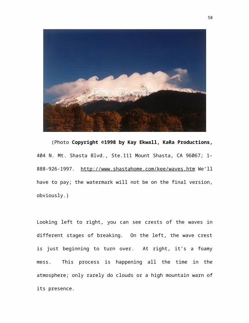
Figure 12.12. Automated observations of wind and pressure at Birmingham, AL during

the February 22, 1998 gravity wave-induced windstorm. [Figure from the Birmingham

NWS Web site: http://www.srh.noaa.gov/bmx/february_22_1998/birmingham.html ]

58

Figure 12.13. A gravity wave train generated ahead of a cold front north of Brownsville,

Texas on March 19, 1998. [Figure from CIMSS Interesting Images Web site:

http://cimss.ssec.wisc.edu/goes/misc/980319.html ]

59

Figure 12.14. Radar image of a record-setting lake-effect snow band over Lake Erie and

Buffalo, New York on December 10, 1995. A total of 38 inches of snow fell in just 24

hours from this band! (What direction do you think the wind is blowing toward at this

time?) Also note the intensification of the lake-effect band just inland, probably due to

turbulence-caused convergence. [ARTISTS: Figure from

http://www.ems.psu.edu/~diercks/hilliker10.jpeg , a student’s senior thesis. Quality is

not what I’d like, but it’s very tough to find a good image of lake-effect for some

reason.]

60

Figure 12.15. A Lake Michigan lake breeze on the afternoon of July 13, 2000, as viewed

from satellite. Notice the absence of cumulus clouds (white dots) in the cool air near the

lake, especially over western Michigan. The discerning eye will also make out straight-

line gravity wave clouds over central Wisconsin. [Figure from SSEC, UW-Madison.]

61

Figure 12.16. River fog in the Ohio River Valley and its tributaries as seen by satellite

on the cool, calm morning of September 20, 1994. The thin white lines are river valleys

reflecting sunlight due to the presence of thick fog. [Image from CIMSS Interesting

Images Web site: http://cimss.ssec.wisc.edu/goes/misc/g8fog.gif ]

62

Figure 12.17. Radar image of a derecho moving through lower Michigan on May 31,

1998. Notice the curved, bowed-out nature of the red area of strongest storms. [Image

from http://www.crh.noaa.gov/grr/basic/other/main_frame_education.html# The loop on

this site might be good for our Web site, too.]

63

Figure 12.18. The barometric pressure trace in Madison, Wisconsin for the period

immediately before, during, and after the wake low windstorm of June 30, 1993. Time

increases left to right in this diagram over a period of several days. The wake low is

indicated by the drastic fall in pressure near the center of the figure. The wiggles prior to

the drop are due to gravity waves. Notice how little change in pressure occurred in the

days before and after the wake low! [ARTISTS: Redraft; the times on the graph are all

wrong because the barograph wasn’t set properly. Also, all the little lines distract from

the pressure trace itself. In the end, all that matters is: 1) the squiggly black line,

reproduce that painstakingly; 2) the top-to-bottom scale of pressure, from 1020 mb to

64

990 mb; and 3) please omit the distracting grid of horizontal and vertical lines, all that’s

needed are horizontal lines denoting 990 mb, 1000 mb, 1010 mb, and 1020 mb.]

65

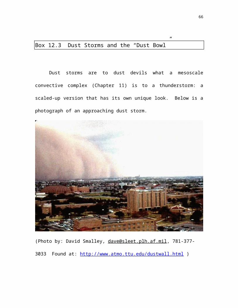
Figure 12.19. The nocturnal low-level jet: a) and b) how it happens, and c) what it looks

like on a Doppler radar velocity plot. In c), the low-level jet is directly above the radar.

The winds are blowing toward (green) the radar to the south and away from (red) the

radar to the north. This low-level jet is 50 miles west of Wichita, Kansas shortly after 10

pm on October 6, 1999, and is about 100 meters directly over the radar and blowing

northward at 10 m/s, or 20 knots. At the same time, the surface winds are calm!

[ARTISTS: model part a) after the Ahrens figure that is pasted-in for Figure 12.2 above.

Change house to something obviously east Texasish. Omit wind gust. Keep eddies and

slowing down of wind above. Part b) should have a moon, quiet winds near the surface,

no eddies going up from the ground, and a fast jet above the surface. Part c) is shown

66

above. Radar image downloaded from

http://www2.etl.noaa.gov/projects/CASESproj.html ]

Figure 12.20. A hand-drawn analysis of a dryline (the front with continuous open half-

circles on it) for a real-life weather situation over west Texas. Compare the dew points

(in red) ahead and behind the dryline. [ARTISTS: will want to redraft and simplify.

Include a few station observations on either side of the funny line with the semicircles on

it; that’s the dryline. Make the numbers on the lower left side of each station observation

RED. Those are dew points. In the end, we’ll want temperature (top left of each station

observation), dew point, and wind direction, plus the dryline. Figure from Tim

Vasquez’s Weather Forecasting Handbook, Weather Graphics Technologies, Garland,

TX, 2000, p. 41.]

67

Figure 12.21. Schematic explaining the mountain and valley breezes. [ARTISTS: model

the graphic almost exactly on Ahrens’s fine figure above, from p. 261 of his 6th edition.]

68

Figure 12.22. [ARTISTS: Help. I need a photograph of one of the bowl-shaped valleys

near Logan, Utah into which bitter cold air sinks in winter. The air is so cold that it kills

off trees, just as cold air at high altitudes kills off trees. The result is a “reverse tree line”

where no trees grow in the bottom of these bowl-valleys. I thought a photograph that

showed these odd, progressively vegetationless bowl valleys might be interesting. I tried,

and failed, to get any such image, or infor, from my Utah meteorology connections. Can

you help? If not, I can try again, since I have a very specific image in mind and I know

who to contact.]

69

Figure 12.23. Winds in the Boulder, Colorado windstorm of December 7, 1987. Notice

how quickly the winds increase, and how consistently strong they are for hours.

[ARTISTS: will probably want to redraft to change units of wind from m/s to mph.

Please reproduce the squiggly line faithfully, though. This graph is from the Univ. of

Colorado’s Web site for weather,

http://weather.colorado.edu/~wxp/labs/windstorms/figures/figure6.html ]

70

Figure 12.24. Two dust devils, large and small, as seen by glider traversing a field in

Arizona. [From Univ. of Arizona Web site devoted to dust devils:

http://www.atmo.arizona.edu/renno/dustdevils.jpg ]

71

Figure 12.25. A lenticular cloud at sunset near Tehachapi, California, as photographed

by the co-author’s student Cynthia Johnson. This smooth, sculpted cloud is a sure sign

of severe mountain-related turbulence nearby. [Cynthia has agreed to this use and should

definitely be paid—this is one of the best all-time lenticular cloud photographs! She’s a

novice photographer shooting pictures in her hometown!]

72

Figure 12.26. The airspeed of a plane flying downwind below the region of lenticular

clouds. Notice the rapid transition from smooth flying to turbulent conditions with wild

fluctuations in airspeed. [ARTISTS: Figure from Peter Lester’s book Turbulence: A

New Perspective for Pilots, Jeppesen/Sanderson, 1994, p. 5-34. Some slight redrafting

necessary, such as changing “10 n. m.” to “11 miles” or omitting it altogether.]

73

Figure 12.27. The Oakland Hills (California) fires of October 20, 1991. [ARTISTS: I

haven’t had much luck finding a good picture of this fire. I would like something with

lots of flames in the image. However, this does illustrate the strong winds, since the

smoke is blown so far downwind. This is from G. Donald Bain’s Web collection of

photos at:

http://www-geoimages.berkeley.edu/GeoImages/BainCalif/CAL400/OAKFIRE.HTML ]

74

Figure 12.28. Satellite image of the smoke plume from the Santa Ana wind-caused Point

Reyes, California fire in October 1995. San Francisco Bay is easily visible just to the

right of the origin of the smoke. [Image from

http://www.sfmuseum.org/hist1/ptreyes.html or from San Francisco State Univ.]

75

Figure 12.29. Large-scale satellite view of the Catalina eddy (the small comma-shaped

swirl in lower center of image) near Los Angeles in October 1995. The white regions are

low-level stratus clouds and fog which the Catalina eddy is pushing onshore (note wind

76

directions). [ARTISTS: Image from San Francisco State University Web site.

Developmental editor wants the eddy labeled; I’ll try to do that at a later stage.]

Figure 12.30. Geographic summary of American small-scale winds. [ARTISTS:

PLEASE redraft and have fun with it. I’m pretty close to the locations I want for each

name. Developmental editor again strongly suggests the use of cool computer-generated

topographic maps.]

77

Figure 12.31. Selected small-scale winds from around the world. Each wind’s American

counterpart is listed in parentheses below the name. [ARTISTS: PLEASE redraft! I did

the best I could. Hope you can read the winds. Specific location of the winds, etc. can

be hashed out with artists; it’s the concept that counts for now. Developmental editor

strongly suggests computer-generated topographic map. Thank you, artists!]

78