Full Terms & Conditions of access and use can be found athttp://www.tandfonline.com/action/journalInformation?journalCode=uasa20

Download by: [University of Minnesota Libraries, Twin Cities] Date: 27 May 2017, At: 15:36

Journal of the American Statistical Association

ISSN: 0162-1459 (Print) 1537-274X (Online) Journal homepage: http://www.tandfonline.com/loi/uasa20

Estimation and Inference of Quantile Regressionfor Survival Data under Biased Sampling

Gongjun Xu, Tony Sit, Lan Wang & Chiung-Yu Huang

To cite this article: Gongjun Xu, Tony Sit, Lan Wang & Chiung-Yu Huang (2016): Estimation andInference of Quantile Regression for Survival Data under Biased Sampling, Journal of the AmericanStatistical Association, DOI: 10.1080/01621459.2016.1222286

To link to this article: http://dx.doi.org/10.1080/01621459.2016.1222286

View supplementary material

Accepted author version posted online: 26Aug 2016.

Submit your article to this journal

Article views: 372

View related articles

View Crossmark data

ACCEPTED MANUSCRIPT

Estimation and Inference of Quantile Regression forSurvival Data under Biased Sampling

Gongjun Xu†, Tony Sit∗, Lan Wang† and Chiung-Yu Huang‡

†School of Statistics, University of Minnesota∗Department of Statistics, The Chinese University of Hong Kong

‡Sidney Kimmel Comprehensive Cancer Center, Johns Hopkins University

xuxxx360@umn.edu tonysit@sta.cuhk.edu.hk wangx346@umn.edu cyhuang@jhu.edu

Abstract

Biased sampling occurs frequently in economics, epidemiology and medical studies ei-

ther by design or due to data collecting mechanism. Failing to take into account the sampling

bias usually leads to incorrect inference. We propose a unified estimation procedure and a

computationally fast resampling method to make statistical inference for quantile regression

with survival data under general biased sampling schemes, including but not limited to the

length-biased sampling, the case-cohort design and variants thereof. We establish the uniform

consistency and weak convergence of the proposed estimator as a process of the quantile level.

We also investigate more efficient estimation using the generalized method of moments and

derive the asymptotic normality. We further propose a new resampling method for inference,

which differs from alternative procedures in that it does not require to repeatedly solve estimat-

ing equations. It is proved that the resampling method consistently estimates the asymptotic

covariance matrix. The unified framework proposed in this paper provides researchers and

practitioners a convenient tool for analyzing data collected from various designs. Simulation

studies and applications to real data sets are presented for illustration.

Keywords: case-cohort sampling; censored quantile regression; length-biased data; resam-

pling; stratified case-cohort sampling; survival time.

1ACCEPTED MANUSCRIPT

ACCEPTED MANUSCRIPT

The first two authors contributed equally to this work. Gongjun Xu is Assistant Professor, School of Statistics, University of

Minnesota, Minneapolis, MN 55455 (E-mail:xuxxx360@umn.edu). Tony Sit is Assistant Professor, Department of Statistics,

The Chinese University of Hong Kong, Hong Kong SAR (E-mail:tonysit@sta.cuhk.edu.hk). Lan Wang is Professor, School

of Statistics, University of Minnesota, Minneapolis, MN 55455 (E-mail:wangx346@umn.edu). Chiung-Yu Huang is Associate

Professor, Division of Biostatistics and Bioinformatics, Sidney Kimmel Comprehensive Cancer Center, Johns Hopkins University,

Baltimore, MD 21205 (E-mail:cyhuang@jhu.edu). The authors thank the editors, the associate editor and two anonymous

referees for their constructive comments that led to substantial improvements. Xu’s work was partially supported by IES Grant

R305D160010; Sit’s work was partially supported ECS-24300514 and GRF-14317716; Wang’s work was partially supported

by NSF DMS-1308960; Huang’s work was sponsored by National Institutes of Health grant 1R01CA193888. The authors

also express gratitude to Professors Ian McDowell, Masoud Asgharian, and Christina Wolfson for kindly sharing the Canadian

Study of Health and Aging (CSHA) data. The core study (CSHA) was funded by the National Health Research and Development

Program (NHRDP) of Health Canada Project 6606-3954-MC(S). Additional funding was provided by Pfizer Canada Incorporated

through the Medical Research Council/Pharmaceutical Manufacturers Association of Canada Health Activity Program, NHRDP

Project 6603-1417-302(R), Bayer Incorporated, and the British Columbia Health Research Foundation Projects 38 (93-2) and 34

(96-1).

2ACCEPTED MANUSCRIPT

ACCEPTED MANUSCRIPT

1 Introduction

Biased sampling occurs frequently, either naturally or by design, in many observational studies.

For example, the cross-sectional prevalent cohort sampling scheme is commonly employed to

study a rare disease. It is well known that the prevalent sampling scheme favors individuals who

survive longer, because diseased individuals who died before the recruitment would not be sam-

pled. As a result, prevalent cases do not comprise a representative sample of the target population.

Problems of this sort can also be found in cross-sectional studies in ecology (McFadden, 1962;

Muttlak and McDonald, 1990; Chen, 2010), industrial quality control (Cox, 1969) and economics

(Kiefer, 1988; Helsen and Schmittlein, 1993; de Una Alvarez, 2004). Another commonly en-

countered biased sampling method is the case-cohort design (Prentice, 1986; Chen, 2001). The

case-cohort design provides an economical approach to conducting epidemiological studies that

involve rare diseases and/or expensive exposures, where covariate information is collected from all

failures but only from a representative sub-sample of censored observations. Various extensions of

the case-cohort design can be found in Borgan et al. (2000), Kulich and Lin (2004) and Samuelsen,

Ånestad, and Skrondal (2007).

Ignoring sampling bias may lead to substantial estimation bias and fallacious inference. This

issue has drawn considerable attentions recently; however, most existing literature focuses on either

the proportional/additive hazards or the accelerated failure time models. For the Cox proportional

hazards (PH) model, estimation procedures under length-biased sampling have been studied in Luo

and Tsai (2009), Qin and Shen (2010) and Huang and Qin (2012); large sample properties for case-

cohort sampling have been developed in Self and Prentice (1988), Lin and Ying (1993) and Chen

and Lo (1999); see also Lu and Tsiatis (2006), Shen, Ning, and Qin (2009) and Kim, Lu, Sit, and

Ying (2013) for corresponding treatments under the linear transformation model, a generalization

of the Cox model. For the accelerated failure time (AFT) model, estimation procedures under

various biased samplings have been discussed in Shen et al. (2009), Kong and Cai (2009), Chen

3ACCEPTED MANUSCRIPT

ACCEPTED MANUSCRIPT

(2010), among others.

In this paper, we propose a general approach for analyzing biased sampling data using quantile

regression. The most prominent feature of quantile regression is its ability to accommodate hetero-

geneous effects of the covariates, which can influence not only the location but also the shape of the

survival time distribution. It is known that the heterogeneity in covariate effects cannot be easily

incorporated in either the Cox PH model or the AFT model. Furthermore, the conditional quantile

of the survival time is easier to interpret than the hazard function and is often of direct interest.

Existing work on censored quantile regression without biased sampling includes Ying, Jung, and

Wei (1995), Portnoy (2003), McKeague, Subramanian, and Sun (2001), Peng and Huang (2008),

Wang and Wang (2009) and many others. For a general introduction to quantile regression, we

refer to Koenker (2005).

Recently, several authors have considered quantile regression under biased sampling. Chen and

Zhou (2012) and Wang and Wang (2014) investigated length-biased data. Both procedures require

estimating the censoring time distribution. Chen and Zhou (2012) assumed a Cox PH model for

the censoring distribution; however, their estimation procedure can lead to biased estimation un-

der a misspecified censoring time distribution. On the other hand, Wang and Wang (2014) relies

on a nonparametric kernel smoothing estimator of the censoring distribution that can suffer from

the curse of dimensionality in practice. For the classical case-cohort sampling scheme, Zheng,

Zhao, and Yu (2013) developed an estimation procedure for quantile regression. These existing

formulations, however, can neither be applied to other biased sampling schemes nor yield efficient

inference on the regression parameters.

The main contribution of this paper is two-fold. First, our formulation offers the first uni-

fied approach for estimating the conditional quantile of the survival time under a variety of bi-

ased sampling schemes, including, in particular, length-biased sampling, case-cohort and stratified

case-cohort designs. We prove that the proposed estimators are consistent and asymptotically nor-

mal. We establish the theory of the regression coefficient estimate as a process of the quantile

4ACCEPTED MANUSCRIPT

ACCEPTED MANUSCRIPT

index while the majority of the literature discusses inference for a fixed (set of) quantiles. Re-

sampling methods are also proposed to construct confidence intervals and the consistency of the

bootstrapping procedure is justified. Second, we show that the efficiency of the proposed estima-

tion procedure can be improved by incorporating additional knowledge about the bias sampling

mechanism. Using length-biased sampling as an example, we demonstrate that an efficient esti-

mate can be obtained by combining estimating equations via the generalized method of moments

(GMM; Hansen, 1982). Compared with Chen and Zhou (2012) and Wang and Wang (2014), the

new approach avoids estimating the nuisance censoring time distribution, which can be challeng-

ing in the case of covariate-dependent censoring. From the application perspective, the unified

solution is expected to benefit a wide range of applications with different types of biased samples.

The codes for simulations and numerical studies, composed inMATLAB, are available upon request.

The rest of the paper is organized as follows. In Section 2.1, we motivate the procedure using

complete data without censoring. In Section 2.2 we present a unified framework for the censored

data under biased sampling; in Section 3 we discuss in detail length-biased and right-censored

data and demonstrate how to improve the estimation efficiency by GMM. Theoretical properties

are studied in Section 4. Sections 5 and 6 present the simulation results and real data sets anal-

ysis, respectively. Section 7 concludes the paper. All the technical proofs are presented in the

supplementary material.

2 Quantile regression under biased sampling

2.1 Complete data without censoring

We first consider the ideal case where the survival time is observed for all subjects. Not only

does this serve to motivate the more technically involved censoring case in Section 2.2 but also is

of independent interest, see for example the applications in Robbins and Zhang (1988), Sun and

5ACCEPTED MANUSCRIPT

ACCEPTED MANUSCRIPT

Woodroofe (1991), Gilbert (2000), and Efromovich (2004).

Let T∗ andZ∗ denote the survival time and thep-dimensional vector of covariates of the target

population. Forτ ∈ (0,1), the conditional quantile function ofT∗ given Z∗ = z is defined as

Q(τ | z) = inf {t : P(T∗ ≤ t | Z∗ = z) ≥ τ}. We consider the following quantile regression model

Q(τ | z) = exp{z>β0(τ)}, for τ ∈ (0,1), (1)

whereβ0(τ) is the vector of unknown quantile regression coefficients describing the effects of

covariatesZ∗ on theτth quantile of logT∗. Compared with the AFT model and the Cox model, the

quantile regression model (1) is more flexible in the sense that the covariate effect is not restricted

to be constant across differentτ’s.

Denote the conditional density, hazard, and cumulative hazard functions ofT∗ givenZ∗ = z by

f (t | z), λ(t | z) andΛ(t | z), respectively. We useA∗, whenever applicable, to denote the time from

the initiation event, such as the onset of a disease, to sampling. Note thatA∗ is often referred to as

the truncation time. LetT, A, andZ be the observed survival time, truncation time, and covariate

vector under a biased sampling scheme, and letfT(t | Z) denote the conditional density ofT given

the covariateZ.

The observed data consist ofn i.i.d. replicates of (T,Z,A), denoted by (Ti ,Z i ,Ai), for i =

1, . . . , n. We consider a general biased sampling scheme (e.g., Kim et al., 2013) where the density

ratio fT(t | Z)/ f (t | Z) is well-defined on the support ofT∗ and there exists a functionw(t) such

that

fT(t | Z) =w(t) f (t | Z)

∫w(s) f (s | Z)ds

. (2)

Here the weight functionw(t) is known for a given study design; moreover, it describes the sam-

pling bias of an observation, that is, it specifies the relationship between the distribution of the

survival timeT∗ in the target population and that of the observed survival timeT.

For random variables (T∗,Z∗) of the target population, it is straightforward to show that the

stochastic processI (T∗ ≤ t) −∫ t

0I (T∗ ≥ t)dΛ(t | Z∗) is a martingale with respect to theσ-filtration

6ACCEPTED MANUSCRIPT

ACCEPTED MANUSCRIPT

Ft containing information up to timet. Hence, we have

E{d I(T∗ ≤ t) − I (T∗ ≥ t)dΛ(t | Z∗) | Z∗} = 0, (3)

where the expectation is taken with respect to the conditional distribution ofT∗ given Z∗. As a

result, in the absence of sampling bias, we can construct consistent estimation procedures based

on Andersen et al. (1993). Under biased sampling, however, replacingT∗ with T yields biased es-

timation. As suggested by the following lemma, unbiased estimating equations can be constructed

by weighing the observations inversely proportional to the sampling weight.

Lemma 1 Under the biased sampling scheme specified in(2), we have

EZ{d I(T ≤ t) − v(t)I (T ≥ t)dΛ(t | Z)} = 0, (4)

where v(∙), the weight function, is

v(t) =w(t)w(T)

, (5)

and, for ease of notation, the conditional expectation EZ is taken with respect to biased sampling

distribution fT(∙ | Z) given covariatesZ.

Equation (4) serves as a basis for constructing unbiased estimating equations for a general

family of biased sampling schemes. In particular, settingvi(t) = w(t)/w(Ti), we have the estimating

equations

n−1/2n∑

i=1

Z i

{

I (Ti ≤ t) −∫ t

0vi(s)I (Ti ≥ s)dΛ(s | Z i)

}

= 0.

Under the quantile regression model (1), we haveΛ(eZ>i β(τ) | Z i) = − log(1− τ) for τ ∈ (0,1). As

in Peng and Huang (2008), replacingt with eZ>i β(τ) in the foregoing estimating equation yields

Sn(β, τ) = n−1/2n∑

i=1

Z i

{

I (Ti ≤ eZ>i β(τ)) −∫ τ

0vi(e

Z>i β(s))I (Ti ≥ eZ>i β(s))dH(s)

}

= 0, (6)

with H(s) = − log(1− s) for 0 ≤ s< 1.

7ACCEPTED MANUSCRIPT

ACCEPTED MANUSCRIPT

If additional knowledge is available about the biased sampling mechanism, other choices of

the weight function based on (5) may be used to derive a more efficient estimator (Section 3). We

consider the following example for an illustration.

Example 1 (Left truncation) Left truncation occurs when individuals come under observation

only when they are event free before the truncation time A∗, that is, T∗ ≥ A∗. Here A∗ is usually

assumed to be conditionally independent of T∗ givenZ∗ (Kalbfleisch and Prentice, 2002, p14).

Under left-truncation, we have

fT(t | Z,A) =I (t ≥ A) f (t | Z)

∫I (s≥ A) f (s | Z)ds

. (7)

Thus the weight function is given by w(t) = I (t ≥ A) and, by noting that w(Ti) = I (Ti ≥ Ai) = 1 in

the observed data, we have vi(t) = I (t ≥ Ai).

In the special case of length-biased sampling, where the truncation time A∗ is uniformly dis-

tributed, the residual lifetime Ti − Ai and the truncation time Ai have an exchangeable joint distri-

bution (Vardi, 1989). By exploiting this special structure, we can show that

EZ{d I(Ti ≤ t)} = EZ{I (t ≥ Ai)I (Ti ≥ t)dΛ(t | Z i)}

= EZ{I (t ≥ Ti − Ai)I (Ti ≥ t)dΛ(t | Z i)}.

It follows that, for anyπ ∈ [0,1], setting vi(t) = πI (t ≥ Ai) + (1 − π)I (t ≥ Ti − Ai) in (6) yields

unbiased estimating equations. Further discussion of this example under right censoring is given

in Section 3.1.

2.2 Proposed method for censored data under biased sampling

We now consider the more challenging case where the survival time is subject to right censoring.

Similar to Section 2.1, we denote byT∗ the survival time in the target population and byC∗ the

censoring time, whereT∗ andC∗ are assumed to be conditionally independent given the covariates

8ACCEPTED MANUSCRIPT

ACCEPTED MANUSCRIPT

Z∗ and the possible truncation timeA∗. For left-truncated and right censored data, one can concep-

tually defineC∗ to be the sum of the underlying truncation timeA∗ and the independent censoring

time that terminates the observation of the residual lifetime beyondA∗ (see Section 3.1 for more

details). LetT∗ = min(T∗,C∗) andΔ∗ = I (T∗ ≤ C∗). The conditional density function of (T∗,Δ∗),

given the corresponding covariatesZ∗, is denoted asfT∗,Δ∗(t, δ | Z∗) for t ≥ 0 andδ ∈ {0,1}.

Under a biased sampling scheme, letT andC be the corresponding survival and censoring

times, respectively. Note that (T,C) has a different distribution from that of (T∗,C∗) due to the

sampling bias. We defineT = min(T,C) andΔ = I (T ≤ C). We assume that the conditional

“mixed” joint density of (T,Δ) givenZ (and possible truncation timeA), fT,Δ(t, δ | Z), satisfies

fT,Δ(t, δ | Z) =w(t, δ) fT∗,Δ∗(t, δ | Z)

∑d∈{0,1}

∫w(s,d) fT∗,Δ∗(s,d | Z)ds

, (8)

wherew(s, δ) is the bias function for sampling. This generalizes the setup in Section 2.1 to incor-

porate right censoring. Many common forms of biased sampling settings fall under the proposed

framework, which includes left-truncation, case-cohort sampling, stratified case-cohort sampling,

and others; see Examples 2∼ 4 below. Formulation (8) resembles the setting of Kim et al. (2013)

which, however, did not consider the length-biased sampling studied in Wang (1991), Asgharian

et al. (2002), Shen et al. (2009) and many others. We consider the length-biased sampling, an im-

portant special case under our framework, in Section 3. More importantly, based on the proposed

framework, we will further study efficient estimation of the model parameters.

As a generalization of (3), (T∗,Δ∗,Z∗) in the target population satisfies

E{dΔ∗I (T∗ ≤ t) − I (T∗ ≥ t)dΛ(t | Z∗) | Z∗} = 0,

where the expectation is taken with respect to (T∗,Δ∗) given Z∗ and, as defined in Section 2.1,

Λ(t | Z∗) denotes the cumulative hazard function ofT∗ givenZ∗ (Andersen et al., 1993). We aim at

constructing the weight functionvi(t) such that the above equation still holds with (T∗,Δ∗) replaced

by (T,Δ). Let Yi(t) = I (Ti ≥ t) andNi(t) = Δi I (Ti ≤ t), i = 1, . . . , n,

9ACCEPTED MANUSCRIPT

ACCEPTED MANUSCRIPT

Lemma 2 Under the biased sampling scheme in(8), we have

EZ{dN(t)} = EZ{v(t)Y(t)dΛ(t | Z)},

where v(∙), the weight function, is given by

v(t) =w(t,1)

w(T,Δ)=

fT∗,Δ∗(T,Δ | Z)

fT,Δ(T,Δ | Z)×

fT,Δ(t,1 | Z)

fT∗,Δ∗(t,1 | Z), (9)

and EZ is the expectation with respect to biased sampling distribution fT,Δ conditional onZ.

In the absence of censoring, that is,C = ∞, we have (T,Δ) ≡ (T,1) and thereforev(∙) reduces to

the form in Lemma 1. Whenvi(t) = w(t,1)/w(Ti ,Δi) for i = 1, . . . , n, we can write

EZ

[n−1/2

n∑

i=1

Z i

{Ni(e

Z>i β0(τ)) −∫ eZ>i β0(τ)

0vi(t)Yi(t)dΛ(t | Z i)

}]= 0.

A change of variable gives

EZ

[n−1/2

n∑

i=1

Z i

{Ni(e

Z>i β0(τ)) −∫ τ

0vi(e

Z>i β0(s))Yi(eZ>i β0(s))dH(s)

}]= 0.

This leads to the following unbiased estimating equations

Sn(β, τ) = n−1/2n∑

i=1

Z i

{

Ni(eZ>i β(τ)) −

∫ τ

0vi(e

Z>i β(s))Yi(eZ>i β(s))dH(s)

}

= 0. (10)

The weight function (9) provides a systematic way to construct the estimating equations for many

biased sampling schemes. We consider some examples below for illustration.

Example 2 (Left truncation and right censoring) Consider the left truncation setting in Exam-

ple 1. Conditional on the truncation time A, we have

fT,Δ(t, δ | Z) =I (A ≤ t) fT∗,Δ∗(t, δ | Z)

∑d∈{0,1}

∫I (A ≤ s) fT∗,Δ∗(s,d | Z)ds

.

Following (9), this implies vi(t) = I (Ai ≤ t). Thus,(10)can be reexpressed as

Sn(β, τ) = n−1/2n∑

i=1

Z i

{

Ni(eZ>i β(τ)) −

∫ τ

0I (Ai ≤ eZ>i β(s))Yi(e

Z>i β(s))dH(s)

}

= 0.

10ACCEPTED MANUSCRIPT

ACCEPTED MANUSCRIPT

Further discussion on this example is provided in Section 3 on efficient estimation.

Example 3 (Case-cohort design)Under the case-cohort design (Prentice, 1986), complete infor-

mation on covariates is collected only for uncensored observations. For censored observations,

suppose that the probability of selecting a censored individual into the sub-cohort is p, p∈ (0,1).

Under this biased sampling, the distribution of(T,Δ) satisfies

fT,Δ(t, δ | Z) ={δ + (1− δ)p} fT∗,Δ∗(t, δ | Z)

∑d∈{0,1}

∫{d + (1− d)p} fT∗,Δ∗(s,d | Z)ds

.

Following (9), vi(t) = 1/{Δi + (1− Δi)p}, and this gives

Sn(β, τ) = n−1/2n∑

i=1

Z i

{

Ni(eZ>i β(τ)) −

∫ τ

0

1Δi + (1− Δi)p

Yi(eZ>i β(s))dH(s)

}

= 0.

Note that the estimating equation has the form in Zheng et al. (2013).

Example 4 (Stratified case-cohort design)The stratified case-cohort design was proposed to im-

prove the efficiency of the traditional case-cohort design (Borgan et al., 2000; Kulich and Lin,

2004), where the probability of selecting a censored observation into the subcohort, p(X), is al-

lowed to depend onX, a vector of covariates that may or may not overlap withZ. As in Example

3, we have

fT,Δ(t, δ | Z) ={δ + (1− δ)p(X)} fT∗,Δ∗(t, δ | Z)

∑d={0,1}{d + (1− d)p(X)} fT∗,Δ∗(s,d | Z)ds

,

which implies that(10)can be constructed with vi(t) = 1/{Δi + (1− Δi)p(X i)}.

2.3 Computation of β(τ)

The proposed estimating equations under different biased sampling schemes share the same generic

form as in (10). Motivated by Peng and Huang (2008), we adopt a grid-based algorithm. The es-

timator ofβ(τ), denoted byβ(τ), is defined as a right-continuous piecewise-constant function that

jumps only on a gridSL(n) = {0 = τ0 < τ1 < ∙ ∙ ∙ < τL(n) = τu < 1},whereτu is some constant subject

11ACCEPTED MANUSCRIPT

ACCEPTED MANUSCRIPT

to certain identifiability constraint due to censoring; see condition C4 in the supplementary mate-

rial. Note that whenτ = 0, from the model assumption (1), we have 0= Q(0 | z) = exp{z>β0(0)}.

Therefore we chooseβ(0) such that exp{z>β(0)} = 0. Let ‖SL(n)‖ = sup1≤k≤L(n) |τk − τk−1|. The

estimateβ(τk) is obtained by sequentially solving the following estimating equation:

n−1/2n∑

i=1

Z i

{Ni(e

Z>i β(τk)) −k−1∑

j=0

vi(eZ>i β(τ j ))Yi(e

Z>i β(τ j ))(H(τ j+1) − H(τ j))}= 0.

Following Peng and Huang (2008), the above equation can be transformed into aL1 optimization

problem which can be be solved using the Barrodale–Roberts algorithm (Barroda and Roberts,

1974). Alternatively, the corresponding optimization subroutine can be implemented easily in

MATLAB via the functionfminsearch. One practical concern is the choice of the grid size in the

sequential procedure. Theoretically, as shown in the proof of Theorem 1, a grid with size of order

o(n−1/2) ensures weak convergence. In the simulation study, we adopt an equally spaced grid with

size 0.01 and find it works satisfactorily for a variety of settings. Alternatively, we may adopt the

estimation procedure based on estimating integral equations proposed in Huang (2010).

3 Efficiency improvement with GMM

In this section, we show that the efficiency of the unified estimation procedure described in Section

2 can be further improved by applying the GMM method (Hansen, 1982). To our best knowledge,

this is the first attempt in the literature to study the efficient estimation for quantile regression

under biased sampling. In Section 3.1 we consider the case where external information about the

sampling mechanism is available. We use length-biased sampling as an example to illustrate how

the external knowledge about the distribution of the underlying truncation time can be incorporated

in the estimation of regression parameters. In Section 3.2, we focus on general biased sampling

scheme and demonstrate that significant efficiency gain can be achieved by properly introducing a

class of weight functions in the estimating procedure.

12ACCEPTED MANUSCRIPT

ACCEPTED MANUSCRIPT

3.1 Efficiency improvement using additional sampling information

When additional knowledge about the biased sampling mechanism is available, it is possible to

incorporate the additional information to improve the estimation efficiency through the generalized

method of moments. Here, we focus on the length-biased sampling example and demonstrate how

an optimal weight function can be determined.

We writeV as the residual lifetime measured from the truncation timeA to failure. SupposeV

is censored byC, whereC is independent of (A,V) conditional onZ, then the observed survival

and censoring times,T andC, can be expressed as

T = A+ V andC = A+ C.

Conditional onZ, the density ofT, fT(t | Z), can be related to the conditional density ofT∗,

f (t | Z), under the stationarity assumption (Lancaster, 1990, Chap. 3)

fT(t | Z) =1

μ(Z)t f (t | Z),

whereμ(Z) =∫

t f (t | Z)dt is a normalizing term. In addition, the joint distribution ofA andV is

(Vardi, 1989)

fA,V(a, v | Z) =1

μ(Z)f (a+ v | Z)I (a > 0, v > 0).

Denote the conditional density and survival functions ofC asgc(t | Z) andSc(t | Z) := P(C >

t | Z). Recall thatTi = min(Ti ,Ci), Δi = I (Ti ≤ Ci), Ni(t) = Δi I (Ti ≤ t) andYi(t) = I (Ti ≥ t).

As shown in Example 2, conditional on the truncation timeA, we can take the weight function

following (9) as

vi(t) =fT∗,Δ∗(Ti ,Δi | Z i)

fT,Δ(Ti ,Δi | Z i)×

fT,Δ(t,1 | Z i)

fT∗,Δ∗(t,1 | Z i)= I (Ai ≤ t). (11)

Here, we defer the derivation of (11) to the supplementary material. It follows that

EZ{dNi(t) − I (Ai ≤ t)Yi(t)Λ(t | Z i)} = 0. (12)

13ACCEPTED MANUSCRIPT

ACCEPTED MANUSCRIPT

We can also construct other weight functions under the stationarity assumption. In particular, as

shown in Huang and Qin (2012),

EZ{dNi(t) − Δi I (Ti − Ai ≤ t)Yi(t)Λ(t | Z i)} = 0. (13)

We can, therefore, define a family of subject-specific weight functions by combining the results in

(12) and (13):

vi(t; π) = πI (Ai ≤ t) + (1− π)Δi I (Ti − Ai ≤ t), (14)

whereπ ∈ [0,1]. It follows directly from (12) and (13) that

EZ

n−1/2

n∑

i=1

Z i

Ni(eZ>i β0(τ)) −

∫ exp{Z>i β0(τ)}

0vi(t; π)Yi(t)dΛ(t | Z i)

= 0, (15)

and a change of variable gives

EZ

n−1/2

n∑

i=1

Z i

{

Ni(eZ>i β0(τ)) −

∫ τ

0vi(e

Z>i β0(s); π)Yi(eZ>i β0(s))dH(s)

} = 0.

This motivates the following estimating equations

Sn(β, τ; π) = n−1/2n∑

i=1

Z i

{

Ni(eZ>i β(τ)) −

∫ τ

0vi(e

Z>i β(s); π)Yi(eZ>i β(s))dH(s)

}

= 0. (16)

The unbiasedness of the above estimating equation holds under covariate-dependent censoring.

Moreover, the proposed method does not need a consistent estimate of the conditional censoring

distribution functionSc(t|Z). This relaxation substantially reduces the computational complexity,

especially when the number of covariates is not small; see the simulation studies in Section 5.

Efficiency improvement using GMM. We now apply the GMM method (Hansen, 1982) to im-

prove the estimation results. Our goal is to determine a best combination of (12) and (13) in the

sense that the resulting standard error of the estimatorβ is minimized. Let

η(β, τ) =

Sn(β, τ; π = 0)

Sn(β, τ; π = 1)

,

14ACCEPTED MANUSCRIPT

ACCEPTED MANUSCRIPT

whereSn(β, τ; π = 0) andSn(β, τ; π = 1) are simply (16) withvi(t; π = 0) = I (Ti − Ai ≤ t) and

vi(t; π = 1) = I (Ai ≤ t), respectively. The GMM estimator ofβ minimizes

η(β, τ)>W(βint, τ)−1η(β, τ),

whereW is a 2p×2p positive definite working covariance matrix, depending on the true parameter

β0(∙), which is usually evaluated at some preliminary consistent estimatorβint(∙). A simple way to

get the initial estimateβint(∙) is to solve (16) withπ = 0.5.

The asymptotically efficient estimatorβeff(τ) is obtained whenW(βint, τ) = var[η(βint, τ)], i.e.,

βeff(τ) = arg minβ

η(β, τ)>var{η(βint, τ)}−1 η(β, τ).

We can estimate var{η(βint, τ)} by the sample covariance matrixη(βint, τ)η(βint, τ)′. This data driven

approach provides a way to construct the optimal linear combination of estimating equations in

η(βint, τ). In Section 5, we demonstrate via simulations the improvement in efficiency by using this

GMM approach.

3.2 Efficiency improvement using additional weight functions

In this section, we show how the efficiency of the estimates can be improved for a general biased

sampling scheme. It follows from Lemma 2 that

EZ{ψ(t)dN(t)} = EZ{ψ(t)v(t)Y(t)dΛ(t | Z)},

whereψ(t) is a weight function that may depend onZ. As a result, estimating equation (10) can be

generalized as

n−1/2n∑

i=1

Z i

{

ψ(Ti)Ni(eZ>i β(τ)) −

∫ τ

0ψ(eZ>i β(s))vi(e

Z>i β(s))Yi(eZ>i β(s))dH(s)

}

= 0. (17)

Thus we can construct a family of weighted estimating equations by considering different choices

of ψ. The possibly data-dependent weight functionψ plays a similar role as the weight function in

15ACCEPTED MANUSCRIPT

ACCEPTED MANUSCRIPT

the rank-based estimating equations in the AFT model (Tsiatis, 1990; Ying, 1993; Jin et al., 2003).

Intuitively, one would consider the optimal choice ofψ that minimizes the asymptotic variance

of the estimates. However, direct estimation of the optimalψ for the quantile regression under

biased sampling is very challenging. This is mainly due to two reasons. First, the optimalψ

involves the derivative of the unknown density function of the failure time. Although estimation

of the derivative in the absence of biased sampling has been studied under the AFT model (e.g.,

Lin and Chen, 2013), a special case of the model (1), the heterogeneity effects of the covariates

under the quantile regression make the problem much more complicated and challenging. Kernel

smoothing techniques may be applied, but their performance can be poor when there are more than

a few covariates and/or there is a large number of quantiles that need to be estimated. Second, the

optimalψ also depends on the sampling weight functionv. This makesψ a study-specific function

for different biased sampling schemes and further complicates the derivation of the optimalψ.

Even for the special case of the AFT model, the optimal weight has not yet been established in the

literature.

To this end, we propose a computationally efficient and robust method to improve the estima-

tion efficiency. Equation (17) provides different estimating equations forβ and, as before, we can

apply the GMM method to improve the estimation from (10). In particular, considerK weight

functions and denoteψ(t) = {ψ1(t), ∙ ∙ ∙ , ψK(t)}>. Let η(β, τ) be the estimating equations for the

given sets of weights, i.e.,

η(β, τ) = n−1/2n∑

i=1

Z i ⊗

{

ψ(Ti)Ni(eZ>i β(τ)) −

∫ τ

0ψ(eZ>i β(s))vi(e

Z>i β(s))Yi(eZ>i β(s))dH(s)

}

, (18)

where⊗ is the Kronecker product. The GMM estimator ofβ(τ) minimizes

η(β, τ)>W(βint, τ)−1η(β, τ),

whereW is a positive definite working covariance matrix, depending on some initial estimator

βint(∙). A simple way to getβint(∙) is to use the estimator from the unweighted estimating equation.

16ACCEPTED MANUSCRIPT

ACCEPTED MANUSCRIPT

Then the asymptotically efficient estimator ofβ(τ), denoted byβeff(τ), is obtained as

βeff(τ) = arg minβ

η(β, τ)>var{η(βint, τ)}−1 η(β, τ). (19)

We again adopt a grid-based algorithm to solveβeff(τ). Specifically, consider the efficient estimator

βeff(τ) at a fixedτ. In the gridSL(n) = {0 = τ0 < τ1 < ∙ ∙ ∙ < τL(n) = τu < 1} used to solve the

unweighted estimating equation, there isτL∗ ∈ SL(n) such thatτL∗ ≤ τ < τL∗+1. For 0= τ0 < τ1 <

∙ ∙ ∙ < τL∗ , we define

η∗(β, τk) = n−1/2n∑

i=1

Z i⊗{ψ(Ti)Ni(e

Z>i β(τk))

−k−1∑

j=0

ψ(eZ>i β(τ j ))vi(eZ>i β(τ j ))Yi(e

Z>i β(τ j )){H(τ j+1) − H(τ j)}}. (20)

To estimateβeff(τ), we chooseβeff(0) such that exp{z>βeff(0)} = 0 and then sequentially estimate

βeff(τk), 1 ≤ k ≤ L∗, by minimizing

η∗(β, τk)>W(βint, τ)

−1η∗(β, τk).

Finally we have efficient estimator forβeff(τ) asβeff(τL∗).

Remark 1 The proposed approach uses a combination of K weight functions{ψ1(t), ∙ ∙ ∙ , ψK(t)} to

approximate the optimal weight functionψ∗. In practice, we may take simple polynomial functions

of t for ψ’s. As K increases, the method is expected to provide a better approximation forψ∗

while introducing additional estimation variation and higher computational cost. In Section 5, we

illustrate through simulations the efficiency improvement.

Remark 2 For the length biased sampling, under the stationarity assumption, we can also con-

struct estimating equations using an unconditional approach which takes the expectation with

respect to V and A. We consider an unconditional version of the weight function vi. Note that

17ACCEPTED MANUSCRIPT

ACCEPTED MANUSCRIPT

setting the weight functionψ(t) =∫ t

0Sc(s | Z i)ds in estimating equation(17)yields

EZ

Ni(eZ>i β0(τ))∫ Ti

0Sc(s | Z i)ds

= EZ

∫ exp(Z>i β0(τ))

0

1∫ t

0Sc(s | Z i)ds

vi(t)Yi(t)dΛ(t | Z i)

=τ

μ(Z i)= EZ

Δiτ∫ Ti

0Sc(s | Z i)ds

.

This leads to the estimating equation

n∑

i=1

Z iΔi∫ Ti

0Sc(s | Z i)ds

{Ni(e

Z>i β(τ)) − τ}= 0,

which is the estimation procedure proposed in Wang and Wang (2014). Similarly, forπ = 1, it

follows from

EZ

[1

tSc(t − Ai | Z i){dNi(t) − vi(t)Yi(t)dΛ(t | Z i)}

]

= 0

and

EZ

∫ exp(Z>i β0(τ))

0

vi(t)Yi(t)tSc(t − Ai | Z i)

dΛ(t | Z i)

=

τ

μ(Z i)= EZ

{Δiτ

TiSc(Ti − Ai | Z i)

}

thatn∑

i=1

Z iΔi

TiSc(Ti − Ai | Z i)

{Ni(e

Z>i β(τ)) − τ}= 0.

We can combine the above unconditional estimating equation with that proposed in the previous

section by applying the GMM method. However, a consistent estimator for the censoring distribu-

tion Sc(∙ | Z) is required for this unconditional estimation procedure. This introduces additional

complexity of the estimation procedure. Hence we do not further pursue the unconditional ap-

proach in this paper.

18ACCEPTED MANUSCRIPT

ACCEPTED MANUSCRIPT

4 Large-sample properties and statistical inference

4.1 Asymptotic properties

We first establish the uniform consistency and weak convergence of the estimatorβ(τ) given in (10)

of Section 2.2 for the general biased sampling scheme. Applying empirical processes techniques,

we investigate the large-sample behavior ofβ(τ) as a process ofτ. The results are summarized in

Theorem 1.

Theorem 1 Assume that Conditions C1–C5 (stated in the online supplemental material) hold. If

limn→∞ ‖SL(n)‖ = 0, for any τl ∈ (0, τu), thensupτ∈[τ`,τu] ‖β(τ) − β0(τ)‖ → 0 in probability. In

addition, if limn→∞ n1/2‖SL(n)‖ = 0, then n1/2{β(τ)−β0(τ)} converges weakly to a Gaussian process

for τ ∈ [τ`, τu].

The covariance structure of the aforementioned Gaussian process and the proof of Theorem

1 are given in the online supplemental material. Next, we state in Theorem 2 the large-sample

property of the proposed efficient estimator described in Section 3.2.

Theorem 2 Consider the GMM efficient estimator given in(19) at τ ∈ [τ`, τu]. Under Conditions

C1–C6, n1/2{βeff(τ) − β0(τ)} converges weakly to a multivariate normal distribution.

Remark 3 Although a sequential procedure (Sections 2.3 and 3.2) is used to estimate the quantile

regression coefficients, similarly to Peng and Huang (2008), the numerical instability ofβ(τ) at

smallτ has little impact on the estimation at largerτ’s; see e.g., Lai and Ying (1988) for a study

of tail instability.

4.2 A new resampling procedure for inference

In this section, we propose a new resampling approach that provides a consistent estimator of

the asymptotic covariance matrix (Theorem 3). The resampling method avoids the difficulty of

19ACCEPTED MANUSCRIPT

ACCEPTED MANUSCRIPT

estimating the unknown density functions of both the survival time and the censoring times in the

asymptotic covariance matrix. It has the flavor of the perturbation approach of Jin et al. (2003) and

Peng and Huang (2008), but enjoys the novel feature that it does not require to repeatedly solve

estimating equations. In particular, it is considerably faster than a more straightforward resampling

method (described in online supplementary material) that directly extends the perturbation idea and

needs to calculate the estimation pathβ∗(∙) many times.

To describe the new resampling procedure, we first introduce some notation. Forb ∈ Rp, define

m(b) = E{ZN(eZ>b)

}, mn(b) =

1n

n∑

i=1

{Z iNi(e

Z>i b)},

m(b) = E{Zv(eZ>b)Y(eZ>b)

}, mn(b) =

1n

n∑

i=1

{Z ivi(e

Z>i b)Yi(eZ>i b)

},

B(b) = E{Z⊗2 fT,Δ(eZ>b,1 | Z) exp(Z>b)

},

J(b) = −E{Z⊗2v(eZ>b) fT(eZ>b | Z) exp(Z>b)

}.

The new method is motivated by the theoretical property of the estimating equation. From equation

(??) in the online supplemental material, we can write

n1/2[m{β(τ)} −m{β0(τ)}] = φ{−Sn(β0, τ)} + op(1).

whereφ(g)(τ) is defined in (??). Theorem 1 shows that√

n{β(τ) − β0(τ)} converges weakly to

a Gaussian process with covariance matrixB{β0(τ)}−1Σ∗[B{β0(τ)}

−1]>, whereΣ∗(τ) denotes the

limiting covariance matrix ofn1/2[m{β(τ)} − m{β0(τ)}]. To evaluate the limiting distribution of√

n{β(τ) − β0(τ)}, one can estimateB{β0(τ)} and the distribution ofn1/2[m{β(τ)} − m{β0(τ)}] as

follows.

(i) Estimation ofB{β0(τ)}. Motivated by Zeng and Lin (2008), we use a perturbation method

to estimateB{β0(τ)}, which is the slope ofmn(∙) with respect toβ(τ). Specifically,M in-

dependent multivariate standard normal variables{γi}i=1,...,M are generated to serve as the

perturbations on the estimatedβ(τ). These perturbed valuesn1/2mn{β(τ) + n−1/2γi} will then

20ACCEPTED MANUSCRIPT

ACCEPTED MANUSCRIPT

be regressed onγi. The resulting slope matrixB{β(τ)}, whosejth row is the jth least square

slope estimate, is a consistent estimator ofB{β0(τ)}.

(ii) Estimation of the distribution of n1/2[m{β(τ)} −m{β0(τ)}]. We derive the following approxi-

mation result forφ{−Sn(β0, τ)} (see (??) in the online supplementary material)

n1/2[m{β(τ)} −m{β0(τ)}]

= −{Sn(β0, τk) − Sn(β0, τk−1)}

−k∑

`=2

k∏

h=`

[I + J{β0(τh−1)B−1{β0(τh−1)}}{H(τh) − H(τh−1)}]

×{Sn(β0, τh−1) − Sn(β0, τh−2)} + op(1) (21)

, φn{−Sn(β0, τ)} + op(1).

The approximation holds uniformly inτ. As a result, we can use the distribution ofφn{−Sn(β0, τ)}

to estimate that ofn1/2[m{β(τ)}−m{β0(τ)}]. The expression (21) ofφn{−Sn(β0, τ)} involves the

unknown matricesB andJ. As in Step (i), we can get estimates forB(β0(τh)) andJ(β0(τh)),

h = 1, . . . , k, by applying the perturbation method formn(∙) andmn(∙), respectively. With the

estimates ofB andJ, we use the perturbed estimating functionsSn(β, τ) to construct an esti-

mator of the distribution ofφn{−Sn(β0, τ)}. Specifically, we show in the proof of Theorem 3

thatφn{−Sn(β, τ)} has the same limiting distribution asφn{−Sn(β0, τ)}. Then we generateMb

(some large number) replicates ofSn(β, τ) and use the corresponding empirical distribution

of φn{−Sn(β, τ)} to estimate that ofφn{−Sn(β0, τ)}.

Combining (i) and (ii), we can use the distribution ofB{β(τ)}−1φn{−Sn(β, τ)} as an estimator of

that of√

n{β(τ) − β0(τ)}. We present the following result which validates inference based on such

resampling procedure.

Theorem 3 Assume Conditions C1–C5 are satisfied. Conditional on the observed data,B{β(τ)}−1φn{−Sn(β, τ)}

converges weakly to the same limiting process of n1/2{β(τ) − β0(τ)} for τ ∈ [τ`, τu], whereτ` ∈

21ACCEPTED MANUSCRIPT

ACCEPTED MANUSCRIPT

(0, τu).

Remark 4 Unlike existing resampling approaches, such as Jin et al. (2003) and Peng and Huang

(2008), our new method does not require to repeatedly solve the estimating equations, which is

quite time consuming in the sequential optimization of the estimating equations; thus our method

is computationally fast. The consistency of the proposed resampling method is established in

Theorem 3 and we can use the resampling percentiles to construct confidence intervals forβ0.

It is worth mentioning that in general, the weak convergence of the resampling estimates may

not directly imply the convergence the bootstrapped moments, such as the covariance matrix, and

additional regularity conditions may be needed to establish such convergence (see, e.g., Kato,

2011; Cheng, 2014).

Remark 5 At the beginning with smallτ values, the estimates forB and J matrices may not be

stable due to the small sample size. In this case, for smallτ values, we may apply the perturbed

resampling method (described in online supplementary material) while for larger values, we adopt

the introduced new estimation procedure.

5 Simulation studies

Length-biased Sampling In the first set of simulations, we consider length-biased sampling. We

generate the survival time from the following log-linear model

logT∗ = Z1β1 + Z2β2 + (1+ γZ1)ε,

whereε follows a normal distribution andγ controls the level of heteroscedasticity. In particular, if

γ is 0, the above model reduces to the classical accelerated failure time model. The corresponding

conditional quantile function is

Qlog(T∗)(τ|Z) = β(0)(τ) + Z1β(1)(τ) + Z2β(2)(τ),

22ACCEPTED MANUSCRIPT

ACCEPTED MANUSCRIPT

whereZ = (Z1,Z2)′, β(0)(τ) = Q(τ), β(1)(τ) = β1 + γQ(τ) = 1+ γQ(τ), β(2)(τ) = β2 = −1 andQ(τ)

denotes theτth quantile ofε. We generateZ1 from a Bernoulli distribution withP(Z1 = 1) = 0.5

andZ2 from a uniform distribution, Unif(−0.5,0.5). The initiation timeA is generated from the

Unif(0,uA) distribution, whereuA > 0 is a constant that exceeds the upper bound ofT∗ such that

P(T∗ ∈ (t ± δ) | A < T∗) = 0 for t > uA and a smallδ > 0. We only retain the pairs withT∗ > A

which results in the length-biased sampleTi = Ai + Vi for i = 1, . . . , n. Due to the conditionally

independent censoring, onlyTi = min(Ti ,Ci) = Ai + min(Vi , Ci) can be observed, fori = 1, . . . , n.

In our study,γ is set as 1;ε is generated from a normal distributionN(0,0.52); uA is set to be

50; andCi is generated from an exponential distribution with rate [1− 0.9I (Z2 > 0)]λ. The value

of λ is chosen according to the prespecified censoring proportions, 20% and 40%. We consider the

weight function specified in (14) and summarize in Table 1 the results for different values ofπ’s

(with πeff corresponding to the GMM estimator) when the censoring rate is 20%.

We observe that the choice ofπ does not affect the biases of the estimators significantly. How-

ever, the standard error associated with the GMM estimator is lower than that of their counterparts

evaluated at other values ofπ, say atπ = 0.00,0.50 or 1.00. In other words, the GMM procedure

improves the efficiency of the proposed estimator. We observe that the performance of the esti-

mator withπ = 0.5 is similar to that of the GMM estimator. In the remaining numerical study,

for computational simplicity with length-biased data, we adoptπ = 0.5 and find it works well in

various scenarios. Note thatπ = 0.5 has an interpretation of striking a good balance between the

two estimating equations (12) and (13), which are set for adjusting biases due to left-truncation and

right censoring respectively. We also observe that the perturbation approach provides a satisfactory

estimate of the standard error of the proposed estimator.

In addition to bias, standard error and mean squared error, Table 2 also summarizes the esti-

mated standard error (SEE) based on the perturbation approach illustrated in Section 4 as well as

the empirical coverage of the 95% Wald-type confidence intervals. For the resampling scheme,

Mb is set to be 500 to estimate the asymptotic variance of the proposed quantile estimator. We

23ACCEPTED MANUSCRIPT

ACCEPTED MANUSCRIPT

ran M = 2,500 perturbed estimated values for evaluatingB and J. For the choice of perturbation

numberM, we have tried different values ofM ranging from 500 to 10,000, and we observed that

the values ofM do not significantly affect the numerical results. On average, the proposed new

method is four times faster than the traditional resampling procedure for cases where the sample

size is 400. For comparison, we also report the estimate which ignores the biases that exist in the

sample and carries out the method in Peng and Huang (2008) without any modification. We denote

this naive estimator asβ(τ)Naive and it is evident that this naive estimator has substantial bias.

The performance of the proposed method is comparable with that of Wang and Wang (2014)

when the number of covariates is small. However, due to the use of kernel smoothing for estimating

the censoring probability, Wang and Wang (2014) is not practical when the censoring distribution

depends on more than two covariates. In the following example, we examine the performance

of the new method in a setting where the censoring distribution depends on four covariates. We

generate random data from

logT∗ = Z1β1 + Z2β2 + Z3β3 + Z4β4 + (1+ γZ1)ε,

whereβ0 = (1,−1,0.5,−0.5)>, Z3’s andZ4’s are generated fromN(1,0.5) andN(−1,0.5) respec-

tively; Z1 andZ2 are generated in the same fashion as we discussed earlier. The censoring times

are assumed to follow a Cox proportional hazard models with covariatesZ` (` = 1, . . . , 4) and

model parameters (0.5,1.0,−0.5,1.0) and the baseline cumulative hazard functionΛ0(c) = −15

to achieve the target censoring rate. We consider sample sizes 500 and 1,000, and 500 iterations

for each case. The estimated standard errors and coverage probabilities are obtained based on 500

perturbed resamplings. It is noteworthy that a larger sample size is needed to ensure more accurate

coverage probabilities when the number of covariates is larger. Table 3 confirms that the proposed

procedure yields unbiased estimates ofβ and consistent estimates of the corresponding variances.

24ACCEPTED MANUSCRIPT

ACCEPTED MANUSCRIPT

Classical case-cohort sampling We generate the survival time from the following log-linear

model

logT = Z1β1 + Z2β2 + ε,

whereε follows a normal distributionN(0,0.52), Z1 follows a Bernoulli distribution with success

probability 0.5 andZ2 follows a uniform distributionUni f (−1,1). The true parameter values

are (1.0,−1.0). The censoring timeCi is generated from an exponential distribution with rate

[1 − 0.9I (Z2 > 0)]λ, whereλ is chosen to achieve a roughly 80% censoring rate. Such a high

level of censoring rate corresponds to cases more natural to apply case-cohort designs (e.g. rare-

disease studies). Cohort sizes of 100 and 200 are drawn by simple random sampling with one-

third of these samples being observed failures. For the resampling scheme,B is set to be 500 to

estimate the asymptotic variance of the proposed estimator. Same as the procedure in length-biased

simulations, an equally spaced grid withSL(n) = 0.01 is selected. These settings are comparable

with those discussed in Zheng et al. (2013) in the sense that the estimates are all but unbiased with

mean squared errors very close to 0.

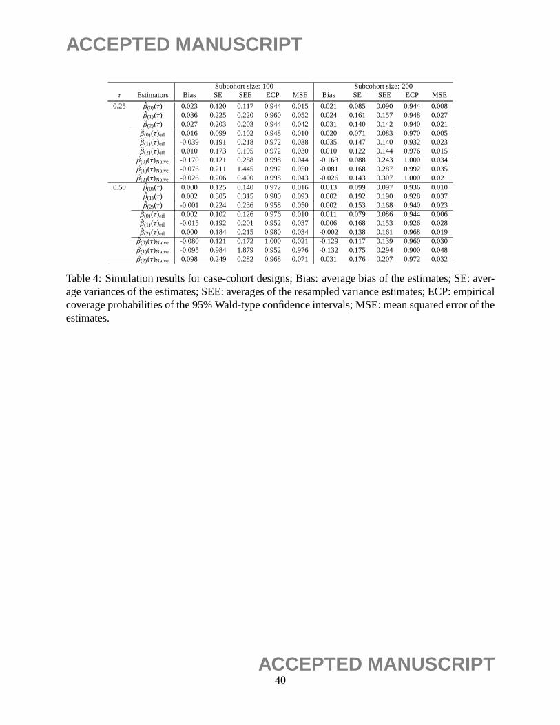
We illustrate through simulations the improvement in efficiency by using additional weight

functions as introduced in Section 3.2. Our numerical study shows that the weight functions,

ψ(t) = (ψ1(t), ψ2(t), ψ3(t)) = (1, t,1/t), generally give stable and improved estimates. Note that the

first weight functionψ1 gives the original estimating equation (10),ψ2 assigns more weights on

survival times around the tail regions, andψ3 puts more weight on shorter survival times. Table 4

summarizes the simulation results. We observe that the GMM-type estimatorβ(τ)eff improves the

efficiency of the estimators significantly, particularly when the subcohort size is smaller. Moreover,

the corresponding SEE’s computed via the proposed resampling method are with good empirical

coverage probabilities.

Stratified case-cohort sampling We generate the survival and censoring times similarly as in the

classical case-cohort sampling example except that the probability of subjects being selected varies

25ACCEPTED MANUSCRIPT

ACCEPTED MANUSCRIPT

according to their covariatesZ’s. Selection probabilities for cases (p1) and censored samples (p2)

are specified as follows:p1(Z) = 1−{1+exp(2.5+0.25Z2)}−1 andp2(Z) = 1−{−1.5+0.5 exp(2Z2)}−1.

Under this setup, about one third of the samples selected are cases while the mean overall censoring

rate is maintained at a level of 75%. We also examined the performance of the efficient estimator

under the stratified case-cohort sampling. The results are summarized in Table 5. Biases are

negligible in all cases and the ECPs are close to their nominal values. For the efficient estimator,

reductions in standard errors ofβ(τ) are also observed.

6 Real data analysis

6.1 Analysis of the CSHA dataset

We first apply the procedure discussed in Section 2.2 to the Canadian Study of Health and Ag-

ing (CSHA) study, which is a multi-center study of the epidemiology of dementia in Canada. It

followed 10,263 senior Canadians over a period from 1991 to 2001 and collected a wide range

of information on their changing health status over time. Amongst these over 10,000 elderly who

were 65 years or older, 1,132 people were identified as having dementia. Excluding subjects with

missing dates of disease onset, we analyze 818 senior individuals that can be classified into three

groups, namely (i) probable Alzheimer’s disease (393 patients), (ii) possible Alzheimer’s disease

(252 patients) and (iii) vascular dementia (252 patients). A total of 180 study subjects among 818

are censored, resulting in a censoring rate about 22%.

Following Wang and Wang (2014), we apply the proposed method to the following model:

Qτ(logTi |zi) = β(0)(τ) + β(1)(τ)z1i + β(2)(τ)z2i , i = 1, . . . , 818,

wherez1i and z2i are dummy variables indicating if theith subject is classified into probably

Alzheimer’s disease or possible Alzheimer’s disease respectively. The vascular dementia group

26ACCEPTED MANUSCRIPT

ACCEPTED MANUSCRIPT

is used as the reference group.

Table 6 summarizes the estimates of the proposed method withπ = 0.5. Again, we obtain very

similar point estimates for different values ofπ. A total of 500 perturbation resampling procedures

are carried out to estimate the standard errors of the estimators, which are presented in parentheses

in the table. Figure 1 demonstrates the estimated quantiles of the three dementia subtypes, where

the vertical lines correspond to the 95% pointwise confidence intervals of the estimated quantiles

of the patients in the baseline group (vascular dementia). Ning et al. (2011) found no significant

difference in survival times among the three types of dementia when considering the mean sur-

vival time with the AFT model. In our analysis, however, we observe that seniors with possible

Alzheimer’s disease tend to have longer survival time than those who suffered from vascular de-

mentia. Such an observation is evident in Figure 1 where the estimated quantiles corresponding

to possible Alzheimer’s disease are not fully covered by the confidence intervals constructed with

respect to the baseline vascular dementia patients. Our results agree with the findings presented in

Wang and Wang (2014).

6.2 Application to case-cohort designs - Welsh nickel refiners study

We now analyze a data set collected in the South Welsh nickel refiners study (Appendix VIII

of Breslow and Day (1987)). The data consist of 679 subjects employed in a nickel refinery.

The goal of the study is to investigate the association between the development of nasal sinuses

and the exposure to nickel. The follow-up through 1981 uncovered 56 deaths from cancer of the

nasal sinus; hence the censoring rate is higher than 90%. Breslow and Day (1987), followed by

Lin and Ying (1993), analyzed the mortality data on the nasal sinus cancer using the Cox model

with (modified) case-cohort design. Previous studies found thatAFE (age at first employment),

YFE (year at first employment) andEXP (exposure level) are significant factors. Lin and Ying

(1993) considered the following regression covariates:log(AFE-10), log of the age of the first

27ACCEPTED MANUSCRIPT

ACCEPTED MANUSCRIPT

employment minus 10 years,(YFE-1915)/10, (YFE-1915)2/100, two transformed versions of

number of years working in the refinery since 1915 andlog(EXP+1), the log exposure level;

some of the subjects had zero exposure and hence EXP+1 is considered so that its logged value is

non-negative and well-defined.

The identifiability of the quantile estimates is only valid up to the 15th quantile due to the fact

that the Kaplan-Meier estimate, based on the full cohort, does not drop further after it reaches 0.85.

We will compare the results obtained from a (i) full cohort, (ii) a subcohort collected under the

traditional setting and (iii) a subcohort collected under stratified case-cohort procedure as described

in Section 2.2. In particular, we usep1 = 1− {1+exp(−1+ LOGAFE)}−1 andp2 = 1− {1+exp(−3+

LOGAFE)}−1 for selecting cases and censored subjects into the sample. This leads to, on average a

sample size of 310. The spaced grid was selected to be of size 0.001 for this numerical studies.

500 resamplings were carried for evaluation of the standard errors of the proposed estimates. We

also applied the methodology introduced in Section 3.2 in order to obtain a more efficient set of

estimates. Similar to our simulation setting, the weight function ofψ(t) = (ψ1(t), ψ2(t), ψ3(t)) =

(1, t,1/t) was applied. It can be observed that, based on the results presented in Table 7, that both

the original and the improved estimates obtained from subcohorts due to classical/stratified case-

cohort samplings are similar to their counterparts based on the full cohort data. The standard errors

of these estimates are also similar.

Figure 2 is included for the purpose of presenting an overall performance of the proposed

method on this nickel refinery dataset. It displays the average point estimates and the corresponding

pointwise standard errors of the four covariates for the 5th, the 10th and the 15th quantiles. It is

noteworthy that the covariatelog(AFE-10) is significant for all the quantiles. This is consistent

with the findings discussed in Lin and Ying (1993) and Kim et al. (2013). Another covariate that

was found to be statistically significant in the two aforementioned literature,log(EXP+1), is also

significant in our study.

28ACCEPTED MANUSCRIPT

ACCEPTED MANUSCRIPT

7 Conclusion and Discussions

Biased sampling arises frequently in many observational studies. Conventional approaches without

accounting for the sampling bias can lead to substantial estimation bias and fallacious inference.

In this paper, we introduce a general quantile regression approach to deal with data collected

from various biased sampling schemes. While our method can handle some specific types of

biased sampling schemes that have been studied in the literature, it also covers more general case-

cohort designs including stratified case-cohort and case-cohort sampling on a length-biased dataset,

length-biased sampling that is proportional to the follow-up time (see Kim et al., 2013), all of which

have not yet been previously investigated. Moreover, the one-size-fit-all formulation provides

practitioners with a convenient tool for quantile regression modeling on their datasets collected

under various sampling schemes. Due to the fact that construction of the estimating equations

does not require an estimate of the censoring time distribution, the proposed method can handle

more complex problems with higher dimensional covariates than the existing methods.

Another major contribution of our work concerns with the efficiency improvement for the quan-

tile regression. When there is additional sampling information, we show that the GMM approach

can be applied to obtain an efficient estimate for length-biased survival data under cross-sectional

sampling. In a more general setting, one can construct a set of weighted estimating equations

so as to seek additional information by combining them via GMM. Numerical results show the

proposed efficient estimates outperforms the existing methods. It is worthwhile to point out that

the proposed method is generic and can be easily extended to other models where the theoreti-

cally optimal weight function is hard to obtain. In particular, it would be interesting to explore the

efficiency improvement in the quantile regression without biased sampling.

The choice of the weight functionv(t) is usually informed by study design and prior knowledge

about the disease incidence process, as seen in many research works on case-control studies and

prevalent cohort studies (see, e.g., Shen et al., 2009; Kong and Cai, 2009; Luo and Tsai, 2009;

29ACCEPTED MANUSCRIPT

ACCEPTED MANUSCRIPT

Chen, 2010; Qin and Shen, 2010; Huang and Qin, 2012; Kim et al., 2013; Zheng et al., 2013).

When the knowledge about biased sampling scheme is not available, a data-driven weight function

may be developed by applying a similar technique considered by Qin et al. (2002); however, the

method requires a multiple-sampling setting, where a unbiased sample must be obtained to ensure

identifiability of the model parameters. Therefore, in the one-sampling setting of the current paper,

neither identifiability nor estimation ofv(t) is available due to the lack of unbiased sample.

There are several other directions that are worth pursuing. One issue of the proposed method,

as discussed in Peng and Huang (2008), is identifiability of upper quantiles due to the abundance of

censored observations towards the tail. This feature is particularly prominent for biased-sampling

cases due to potentially high censoring rates as we have seen in case-cohort designs for instance.

It is of interest to incorporate the method of Portnoy (2014) in the current set up and investigate

the benefits of jackknife under various biased-sampling settings.

30ACCEPTED MANUSCRIPT

ACCEPTED MANUSCRIPT

References

Andersen, P. K., Borgan, Ø., Gill, R. D., and Keiding, N. (1993),Statistical Models Based on

Counting Processes, Springer, New York.

Asgharian, M., M’Lan, C. E., and Wolfson, D. B. (2002), “Length-Biased Sampling with Right

Censoring: An Unconditional Approach,”Journal of the American Statistical Association, 97,

201–209.

Barroda, I. and Roberts, F. (1974), “Solution of an Overdetermined System of Equations in the L1

Norm,” Communications of the ACM, 17, 319–320.

Borgan, O., Langholz, B., Samuelsen, S. O., Goldstein, L., and Pogoda, J. (2000), “Exposure

Stratified Case-Cohort Designs,”Lifetime Data Analysis, 6, 39–58.

Breslow, N. and Day, N. (1987),Statistical Methods in Cancer Research, Vol. II: The Design and

Analysis of Cohort Studies, Lyon, France: IARC.

Chen, K. (2001), “Generalized Case-Cohort Sampling,”Journal of the Royal Statistical Society:

Series B, 63, 791–908.

Chen, K. and Lo, S.-H. (1999), “Case-Cohort and Case-Control Analysis with Cox’s Model,”

Biometrika, 86, 755–764.

Chen, X. and Zhou, Y. (2012), “Quantile Regression for Right-Censored and Length-Biased Data,”

Acta Mathematicae Applicatae Sinica, 28, 443–462.

Chen, Y. Q. (2010), “Semiparametric Regression in Size-Biased Sampling,”Biometrics, 66, 149–

158.

Cheng, G. (2014), “Moment Consistency of the Exchangeably Weighted Bootstrap for Semipara-

metric M-estimation,”Scandinavian Journal of Statistics, Forthcoming.

31ACCEPTED MANUSCRIPT

ACCEPTED MANUSCRIPT

Cox, D. (1969),Some Sampling Problems in Technology, eds. Johnson and Smith, New York:

Wiley.

de UnaAlvarez, J. (2004), “Nonparametric Estimation under Length-Biased Sampling and Type I

Censoring: a Moment-Based Approach,”Annals of the Institute of Statistical Mathematics, 56,

667–681.

Efromovich, S. (2004), “Density Estimation for Biased Data,”Annals of Statistics, 32, 1137–1161.

Gilbert, P. B. (2000), “Large Sample Theory of Maximum Likelihood Estimates in Semiparametric

Biased Sampling Models,”Annals of Statistics, 28, 151–194.

Hansen, L. P. (1982), “Large Sample Properties of Generalized Method of Moments Estimators,”

Econometrica, 50, 1029–1054.

Helsen, K. and Schmittlein, D. (1993), “Analyzing Duration Times in Marketing: Evidence for the

Effectiveness of Hazard Rate Models,”Marketing Science, 11, 395–414.

Huang, C.-Y. and Qin, J. (2012), “Composite Partial Likelihood Estimation Under Length-Biased

Sampling, with Application to a Prevalent Cohort Study of Dementia,”Journal of the American

Statistical Association, 107, 946–957.

Huang, Y. (2010), “Quantile Calculus and Censored Regression,”The Annals of Statistics, 38,

1607–37.

Jin, Z., Lin, D. Y., Wei, L. J., and Ying, Z. (2003), “Rank-Based Inference for the Accelerated

Failure Time Model,”Biometrika, 90, 341–353.

Kalbfleisch, J. D. and Prentice, R. L. (2002),The Statistical Analysis of Failure Time Data, Wiley,

New York.

32ACCEPTED MANUSCRIPT

ACCEPTED MANUSCRIPT

Kato, K. (2011), “A note on moment convergence of bootstrap M-estimators,”Statistics& Deci-

sions, 28, 51–61.

Kiefer, N. M. (1988), “Economic Duration Data and Hazard Functions,”Journal of Economic

Literature, 26, 646–679.

Kim, J. P., Lu, W., Sit, T., and Ying, Z. (2013), “A Unified Approach to Semiparametric Transfor-

mation Models Under General Biased Sampling Schemes,”Journal of the American Statistical

Association, 108, 217–227.

Koenker, R. (2005),Quantile Regression, Cambridge University Press.

Kong, L. and Cai, J. (2009), “Case–Cohort Analysis with Accelerated Failure Time Model,”Bio-

metrics, 65, 135–142.

Kulich, M. and Lin, D. (2004), “Improving the Efficiency of Relative-Risk Estimation in Case-

Cohort Studies,”Journal of the American Statistical Association, 99, 832–844.

Lai, T. L. and Ying, Z. (1988), “Stochastic Integrals of Empirical-Type Processes with Applications

to Censored Regression,”Journal of Multivariate Analysis, 27, 334–358.

Lancaster, T. (1990),The Econometric Analysis of Transition Data, Cambridge university press.

Lin, D. and Ying, Z. (1993), “Cox Regression with Incomplete Covariate Measurements,”Journal

of the American Statistical Association, 88, 1341–1349.

Lin, Y. Y. and Chen, K. (2013), “Efficient Estimation of the Censored Linear Regression Model,”

Biometrika, 100, 525–30.

Lu, W. and Tsiatis, A. (2006), “Semiparametric Transformation Models for the Case-Cohort

Study,”Biometrika, 93, 207–214.

33ACCEPTED MANUSCRIPT

ACCEPTED MANUSCRIPT

Luo, X. and Tsai, W. Y. (2009), “Nonparametric Estimation for Right-Censored Length-Biased

Data: a Pseudo-partial Likelihood Approach,”Biometrika, 96, 873–886.

McFadden, J. (1962), “On the Lengths of Intervals in a Stationary Point Process,”Journal of the

Royal Statistical Society, Series B, 24, 364–382.

McKeague, I. W., Subramanian, S., and Sun, Y. (2001), “Median Regression and the Missing

Information Principle,”Journal of Nonparametric Statistics, 13, 709–727.

Muttlak, H. and McDonald, L. (1990), “Ranked Set Sampling with Size-Biased Probability of

Selection,”Biometrics, 46, 435–446.

Ning, J., Qin, J., and Shen, Y. (2011), “Buckley-James-Type Estimator with Right Censored and

Length-Biased Data,”Biometrics, 67, 1369–1378.

Peng, L. and Huang, Y. (2008), “Survival Analysis with Quantile Regression Models,”Journal of

the American Statistical Association, 103, 637–649.

Portnoy, S. (2003), “Censored Regression Quantiles,”Journal of the American Statistical Associ-

ation, 98, 1001–1012.

— (2014), “The Jackline’s Edge: Inference for Censored Regression Quantiles,”Computational

Statistics and Data Analysis, 72, 273–281.

Prentice, R. L. (1986), “A Case-Cohort Design for Epidemiologic Cohort Studies and Disease

Prevention Trials,”Biometrika, 73, 1–11.

Qin, J., Berwick, M., Ashbolt, R., and Dwyer, T. (2002), “Quantifying the Change of Melanoma

Incidence by Breslow Thickness,”Biometrics, 58, 665–670.

Qin, J. and Shen, Y. (2010), “Statistical Methods for Analyzing Right-Censored Length-Biased

Data under Cox Model,”Biometrics, 66, 382–392.

34ACCEPTED MANUSCRIPT

ACCEPTED MANUSCRIPT

Robbins, H. and Zhang, C.-H. (1988), “Estimating a Treatment Effect under Biased Sampling,”

Proceedings of the National Academy of Sciences, 85, 3670–3672.

Samuelsen, S., Ånestad, H., and Skrondal, A. (2007), “Stratified Case-Cohort Analysis of General

Cohort Sampling Designs,”Scandinavian Journal of Statistics, 34, 103–119.

Self, S. G. and Prentice, R. L. (1988), “Asymptotic Distribution Theory and Efficiency Results for

Case-Cohort Studies,”The Annals of Statistics, 16, 64–81.

Shen, Y., Ning, J., and Qin, J. (2009), “Analyzing Length-Biased Data with Semiparametric Trans-

formation and Accelerated Failure Time Models,”Journal of the American Statistical Associa-

tion, 104, 1192–1202.

Sun, J. and Woodroofe, M. (1991), “Semi-Parametric Estimates under Biased Sampling,”Statistica

Sinica, 7, 545–575.

Tsiatis, A. A. (1990), “Estimating Regression Parameters Using Linear Rank Tests for Censored

Data,”The Annals of Statistics, 18, 354–372.

Vardi, Y. (1989), “Multiplicative Censoring, Renewal Processes, Deconvolution and Decreasing

Density: Nonparametric Estimation,”Biometrika, 76, 751–761.

Wang, H. and Wang, L. (2014), “Quantile Regression Analysis of Length-Biased Survival Data,”

Stats, 3, 31–47.

Wang, H. J. and Wang, L. (2009), “Locally Weighted Censored Quantile Regression,”Journal of

the American Statistical Association, 104, 1117–1128.

Wang, M.-C. (1991), “Nonparametric Estimation from Cross-sectional Survival Data,”Journal of

the American Statistical Association, 86, 130–143.

35ACCEPTED MANUSCRIPT

ACCEPTED MANUSCRIPT

Ying, Z. (1993), “A Large Sample Study of Rank Estimation for Censored Regression Data,”The

Annals of Statistics, 21, 76–99.

Ying, Z., Jung, S. H., and Wei, L. J. (1995), “Survival Analysis with Median Regression Models,”

Journal of the American Statistical Association, 90, 178–184.

Zeng, D. and Lin, D. (2008), “Efficient Resampling Methods for Nonsmooth Estimating Func-

tions,” Biostatistics, 9, 355–363.

Zheng, M., Zhao, Z., and Yu, W. (2013), “Quantile Regression Analysis of Case-Cohort Data,”

Journal of Multivariate Analysis, 122, 20–34.

36ACCEPTED MANUSCRIPT

ACCEPTED MANUSCRIPT

n = 200 n = 400π τ Estimators Bias SE MSE Bias SE MSE

0.00 0.25 β(0)(τ) -0.033 0.297 0.089 -0.047 0.184 0.036β(1)(τ) -0.087 0.511 0.269 0.032 0.346 0.121β(2)(τ) 0.022 0.308 0.095 0.002 0.176 0.031

0.50 β(0)(τ) -0.026 0.226 0.052 -0.020 0.108 0.012β(1)(τ) -0.054 0.356 0.129 0.009 0.234 0.055β(2)(τ) 0.021 0.243 0.059 -0.001 0.125 0.016

0.50 0.25 β(0)(τ) -0.023 0.254 0.065 -0.030 0.174 0.031β(1)(τ) -0.062 0.481 0.236 0.011 0.334 0.112β(2)(τ) 0.005 0.260 0.068 -0.008 0.169 0.029

0.50 β(0)(τ) -0.014 0.142 0.020 -0.012 0.115 0.013β(1)(τ) -0.034 0.319 0.103 0.000 0.231 0.053β(2)(τ) 0.008 0.167 0.028 -0.009 0.123 0.015

1.00 0.25 β(0)(τ) -0.048 0.287 0.084 -0.035 0.191 0.038β(1)(τ) -0.046 0.582 0.341 -0.019 0.365 0.133β(2)(τ) 0.016 0.286 0.082 0.010 0.191 0.036

0.50 β(0)(τ) -0.027 0.168 0.029 -0.014 0.123 0.015β(1)(τ) -0.028 0.353 0.125 -0.009 0.253 0.064β(2)(τ) 0.014 0.203 0.041 0.001 0.128 0.016

πeff 0.25 β(0)(τ) -0.044 0.198 0.041 -0.045 0.154 0.026β(1)(τ) 0.039 0.389 0.153 -0.090 0.304 0.100β(2)(τ) -0.036 0.176 0.032 0.078 0.130 0.023

0.50 β(0)(τ) 0.010 0.136 0.019 -0.009 0.091 0.008β(1)(τ) 0.067 0.263 0.073 -0.085 0.210 0.051β(2)(τ) -0.076 0.124 0.021 0.041 0.100 0.012

Table 1: Simulation results for length-biased data (20% censoring rate) for different values ofπ(πeff corresponds to the GMM estimator). Bias: average bias of the estimate; SE: average varianceof the estimate; MSE: mean squared error of the estimate.

37ACCEPTED MANUSCRIPT

ACCEPTED MANUSCRIPT

n = 200 n = 400Censoring τ Estimators Bias SE SEE ECP MSE Bias SE SEE ECP MSE

20% 0.25 β(0)(τ) -0.042 0.248 0.283 0.972 0.063 -0.005 0.130 0.128 0.956 0.035β(1)(τ) -0.014 0.486 0.503 0.952 0.256 -0.043 0.304 0.331 0.970 0.122β(2)(τ) -0.004 0.255 0.244 0.944 0.065 0.001 0.129 0.114 0.928 0.031

β(0)(τ)Naive 0.307 0.117 0.095 0.212 0.108 0.166 0.048 0.085 0.400 0.030β(1)(τ)Naive 0.854 0.230 0.160 0.148 0.756 0.814 0.085 0.120 0.000 0.670β(2)(τ)Naive 0.270 0.349 0.337 0.820 0.199 0.054 0.274 0.236 0.878 0.078

0.50 β(0)(τ) -0.016 0.145 0.185 0.966 0.021 -0.014 0.111 0.130 0.966 0.012β(1)(τ) 0.020 0.323 0.363 0.962 0.105 -0.001 0.229 0.283 0.982 0.052β(2)(τ) -0.013 0.168 0.150 0.926 0.028 0.007 0.114 0.104 0.924 0.013

β(0)(τ)Naive 0.302 0.039 0.049 0.890 0.002 0.000 0.004 0.049 0.900 0.000β(1)(τ)Naive 0.277 0.172 0.170 0.652 0.121 -0.555 0.042 0.085 0.000 0.309β(2)(τ)Naive 0.141 0.322 0.295 0.856 0.123 0.002 0.263 0.253 0.978 0.069

40% 0.25 β(0)(τ) -0.033 0.238 0.263 0.966 0.063 -0.008 0.132 0.125 0.950 0.036β(1)(τ) 0.022 0.511 0.505 0.936 0.256 -0.031 0.312 0.291 0.936 0.112β(2)(τ) -0.007 0.244 0.215 0.920 0.065 0.003 0.126 0.118 0.958 0.031

β(0)(τ)Naive 0.261 0.114 0.130 0.472 0.081 0.248 0.087 0.088 0.248 0.069β(1)(τ)Naive 0.890 0.177 0.194 0.004 0.823 0.891 0.128 0.132 0.000 0.811β(2)(τ)Naive 0.262 0.347 0.364 0.886 0.189 0.283 0.236 0.251 0.806 0.136

0.50 β(0)(τ) -0.011 0.142 0.188 0.964 0.020 -0.012 0.117 0.129 0.952 0.013β(1)(τ) 0.041 0.315 0.362 0.968 0.101 0.006 0.237 0.280 0.968 0.054β(2)(τ) -0.025 0.166 0.155 0.938 0.028 0.001 0.111 0.105 0.922 0.013

β(0)(τ)Naive 0.250 0.124 0.127 0.466 0.078 0.248 0.080 0.088 0.206 0.068β(1)(τ)Naive 1.017 0.200 0.202 0.000 1.074 1.020 0.134 0.140 0.000 1.059β(2)(τ)Naive 0.522 0.360 0.380 0.724 0.402 0.549 0.249 0.263 0.452 0.363

Table 2: Simulation results for length-biased data (20% and 40% censoring rates); Bias: estimatedbias of the estimates; SE: estimated variances of the estimates; SEE: averages of the resampledvariance estimates; ECP: empirical coverage probabilities of the 95% Wald-type confidence inter-vals; MSE: mean squared error of the estimates.

38ACCEPTED MANUSCRIPT

ACCEPTED MANUSCRIPT

n = 500 n = 1000τ Estimators Bias SE SEE ECP MSE Bias SE SEE ECP MSE

0.25 β(0)(τ) 0.008 0.269 0.224 0.936 0.072 -0.026 0.203 0.184 0.956 0.042β(1)(τ) -0.026 0.189 0.174 0.940 0.036 -0.033 0.115 0.127 0.960 0.014β(2)(τ) 0.003 0.311 0.319 0.952 0.097 0.011 0.221 0.222 0.956 0.049β(3)(τ) -0.023 0.165 0.158 0.932 0.028 0.000 0.121 0.119 0.928 0.015β(4)(τ) 0.012 0.178 0.157 0.926 0.032 0.000 0.123 0.119 0.928 0.015

β(0)(τ)Naive 0.369 0.171 0.167 0.396 0.165 0.357 0.108 0.121 0.152 0.139β(1)(τ)Naive 0.693 0.096 0.101 0.000 0.489 0.693 0.064 0.070 0.000 0.484β(2)(τ)Naive 0.094 0.177 0.189 0.912 0.040 0.084 0.119 0.129 0.896 0.021β(3)(τ)Naive -0.047 0.098 0.104 0.936 0.012 -0.039 0.070 0.072 0.920 0.006β(4)(τ)Naive 0.049 0.105 0.104 0.928 0.013 0.050 0.068 0.073 0.896 0.007

0.50 β(0)(τ) -0.001 0.163 0.180 0.964 0.027 0.011 0.107 0.114 0.982 0.012β(1)(τ) -0.038 0.127 0.125 0.948 0.018 -0.048 0.087 0.076 0.946 0.008β(2)(τ) 0.021 0.213 0.226 0.964 0.046 0.010 0.139 0.152 0.954 0.019β(3)(τ) -0.011 0.116 0.108 0.932 0.014 -0.011 0.072 0.079 0.964 0.005β(4)(τ) 0.005 0.122 0.108 0.928 0.015 0.006 0.080 0.080 0.962 0.006

β(0)(τ)Naive 0.404 0.229 0.209 0.504 0.215 0.006 0.212 0.114 0.676 0.045β(1)(τ)Naive 0.674 0.096 0.098 0.000 0.463 0.238 0.079 0.101 0.284 0.063β(2)(τ)Naive 0.157 0.165 0.177 0.868 0.052 0.060 0.155 0.161 0.956 0.028β(3)(τ)Naive -0.056 0.110 0.107 0.908 0.015 -0.059 0.103 0.082 0.880 0.014β(4)(τ)Naive 0.071 0.109 0.111 0.912 0.017 0.064 0.101 0.082 0.860 0.014

Table 3: Simulation results for length-biased data with censoring times generated from a Cox pro-portional hazard model with four covariates; Bias: simulated bias of the estimates; SE: simulatedvariances of the estimates; SEE: averages of the resampled variance estimates; ECP: empiricalcoverage probabilities of the 95% Wald-type confidence intervals; MSE: mean squared errors ofthe estimates.

39ACCEPTED MANUSCRIPT

ACCEPTED MANUSCRIPT

Subcohort size:100 Subcohort size: 200τ Estimators Bias SE SEE ECP MSE Bias SE SEE ECP MSE

0.25 β(0)(τ) 0.023 0.120 0.117 0.944 0.015 0.021 0.085 0.090 0.944 0.008β(1)(τ) 0.036 0.225 0.220 0.960 0.052 0.024 0.161 0.157 0.948 0.027β(2)(τ) 0.027 0.203 0.203 0.944 0.042 0.031 0.140 0.142 0.940 0.021β(0)(τ)eff 0.016 0.099 0.102 0.948 0.010 0.020 0.071 0.083 0.970 0.005β(1)(τ)eff -0.039 0.191 0.218 0.972 0.038 0.035 0.147 0.140 0.932 0.023β(2)(τ)eff 0.010 0.173 0.195 0.972 0.030 0.010 0.122 0.144 0.976 0.015β(0)(τ)Naive -0.170 0.121 0.288 0.998 0.044 -0.163 0.088 0.243 1.000 0.034β(1)(τ)Naive -0.076 0.211 1.445 0.992 0.050 -0.081 0.168 0.287 0.992 0.035β(2)(τ)Naive -0.026 0.206 0.400 0.998 0.043 -0.026 0.143 0.307 1.000 0.021

0.50 β(0)(τ) 0.000 0.125 0.140 0.972 0.016 0.013 0.099 0.097 0.936 0.010β(1)(τ) 0.002 0.305 0.315 0.980 0.093 0.002 0.192 0.190 0.928 0.037β(2)(τ) -0.001 0.224 0.236 0.958 0.050 0.002 0.153 0.168 0.940 0.023β(0)(τ)eff 0.002 0.102 0.126 0.976 0.010 0.011 0.079 0.086 0.944 0.006β(1)(τ)eff -0.015 0.192 0.201 0.952 0.037 0.006 0.168 0.153 0.926 0.028β(2)(τ)eff 0.000 0.184 0.215 0.980 0.034 -0.002 0.138 0.161 0.968 0.019β(0)(τ)Naive -0.080 0.121 0.172 1.000 0.021 -0.129 0.117 0.139 0.960 0.030β(1)(τ)Naive -0.095 0.984 1.879 0.952 0.976 -0.132 0.175 0.294 0.900 0.048β(2)(τ)Naive 0.098 0.249 0.282 0.968 0.071 0.031 0.176 0.207 0.972 0.032

Table 4: Simulation results for case-cohort designs; Bias: average bias of the estimates; SE: aver-age variances of the estimates; SEE: averages of the resampled variance estimates; ECP: empiricalcoverage probabilities of the 95% Wald-type confidence intervals; MSE: mean squared error of theestimates.

40ACCEPTED MANUSCRIPT

ACCEPTED MANUSCRIPT

Subcohort size:200 Subcohort size: 400τ Estimators Bias SE SEE ECP MSE Bias SE SEE ECP MSE

0.25 β(0)(τ) 0.071 0.131 0.137 0.940 0.031 0.047 0.096 0.122 0.980 0.011β(1)(τ) 0.058 0.103 0.096 0.950 0.014 0.057 0.070 0.082 0.949 0.008β(2)(τ) -0.058 0.142 0.140 0.940 0.024 -0.063 0.090 0.108 0.934 0.012β(0)(τ)eff 0.014 0.030 0.042 0.980 0.001 0.018 0.034 0.036 0.938 0.001β(1)(τ)eff -0.027 0.095 0.084 0.940 0.010 0.003 0.082 0.064 0.934 0.007β(2)(τ)eff -0.003 0.128 0.102 0.944 0.016 -0.008 0.072 0.105 0.970 0.005β(0)(τ)Naive -0.193 0.069 0.180 0.980 0.042 -0.202 0.054 0.133 0.794 0.044β(1)(τ)Naive -0.073 0.060 0.125 0.986 0.009 -0.080 0.047 0.094 0.932 0.009β(2)(τ)Naive 0.086 0.094 0.133 0.974 0.016 0.087 0.074 0.100 0.932 0.013

0.50 β(0)(τ) 0.027 0.115 0.115 0.964 0.014 0.053 0.107 0.127 0.948 0.014β(1)(τ) 0.006 0.082 0.088 0.984 0.007 0.018 0.068 0.077 0.974 0.005β(2)(τ) 0.000 0.154 0.148 0.960 0.024 -0.013 0.105 0.117 0.970 0.011β(0)(τ)eff 0.004 0.030 0.044 0.964 0.001 0.011 0.031 0.035 0.950 0.001β(1)(τ)eff -0.004 0.098 0.081 0.972 0.010 0.018 0.080 0.063 0.924 0.007β(2)(τ)eff -0.014 0.085 0.103 0.964 0.007 0.001 0.077 0.103 0.976 0.006β(0)(τ)Naive -0.194 0.102 0.120 0.696 0.048 -0.220 0.072 0.095 0.222 0.054β(1)(τ)Naive -0.071 0.078 0.083 0.930 0.011 -0.087 0.055 0.067 0.772 0.011β(2)(τ)Naive 0.082 0.100 0.105 0.888 0.017 0.092 0.077 0.082 0.792 0.015

Table 5: Simulation results for stratified case-cohort designs; Bias: average bias of the estimates;Var: average variances of the estimates; Est Var: averages of the resampled variance estimates;ECP: empirical coverage probabilities of the 95% Wald-type confidence intervals; MSE: meansquared error of the estimates.

41ACCEPTED MANUSCRIPT

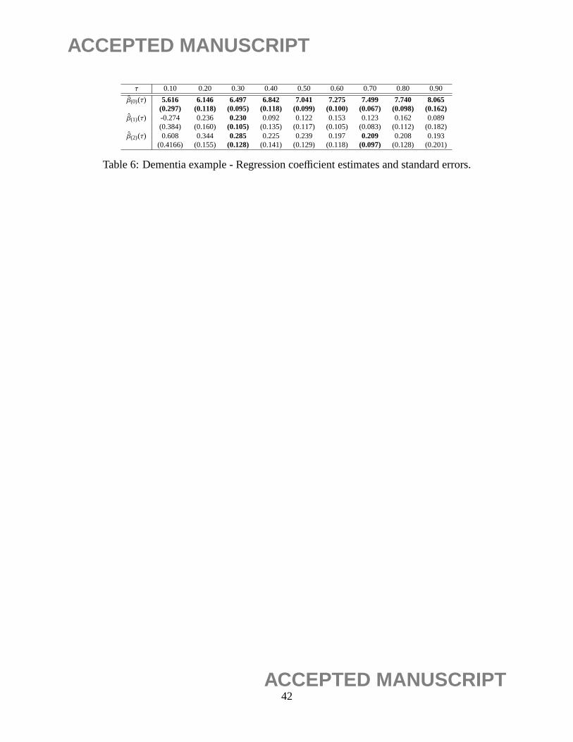
ACCEPTED MANUSCRIPT

τ 0.10 0.20 0.30 0.40 0.50 0.60 0.70 0.80 0.90

β(0)(τ) 5.616 6.146 6.497 6.842 7.041 7.275 7.499 7.740 8.065(0.297) (0.118) (0.095) (0.118) (0.099) (0.100) (0.067) (0.098) (0.162)

β(1)(τ) -0.274 0.236 0.230 0.092 0.122 0.153 0.123 0.162 0.089(0.384) (0.160) (0.105) (0.135) (0.117) (0.105) (0.083) (0.112) (0.182)

β(2)(τ) 0.608 0.344 0.285 0.225 0.239 0.197 0.209 0.208 0.193(0.4166) (0.155) (0.128) (0.141) (0.129) (0.118) (0.097) (0.128) (0.201)

Table 6: Dementia example - Regression coefficient estimates and standard errors.

42ACCEPTED MANUSCRIPT

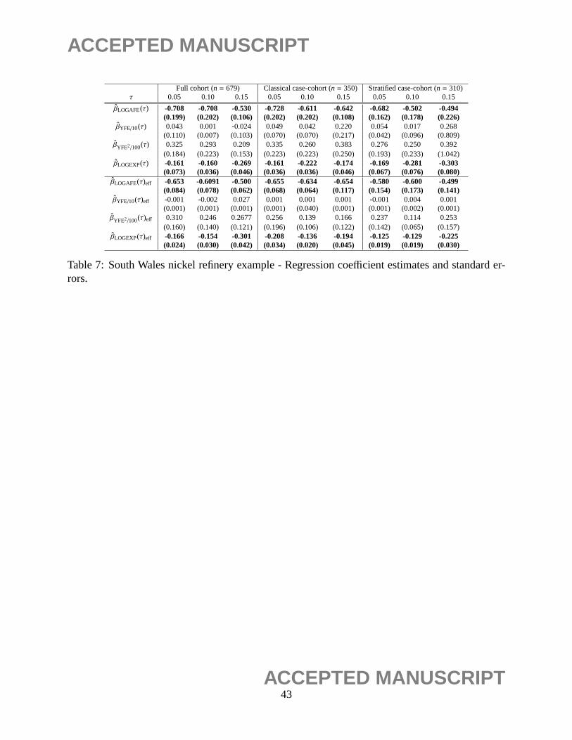
ACCEPTED MANUSCRIPT

Full cohort (n = 679) Classical case-cohort (n = 350) Stratified case-cohort (n = 310)τ 0.05 0.10 0.15 0.05 0.10 0.15 0.05 0.10 0.15

βLOGAFE(τ) -0.708 -0.708 -0.530 -0.728 -0.611 -0.642 -0.682 -0.502 -0.494(0.199) (0.202) (0.106) (0.202) (0.202) (0.108) (0.162) (0.178) (0.226)

βYFE/10(τ) 0.043 0.001 -0.024 0.049 0.042 0.220 0.054 0.017 0.268(0.110) (0.007) (0.103) (0.070) (0.070) (0.217) (0.042) (0.096) (0.809)

βYFE2/100(τ) 0.325 0.293 0.209 0.335 0.260 0.383 0.276 0.250 0.392(0.184) (0.223) (0.153) (0.223) (0.223) (0.250) (0.193) (0.233) (1.042)

βLOGEXP(τ) -0.161 -0.160 -0.269 -0.161 -0.222 -0.174 -0.169 -0.281 -0.303(0.073) (0.036) (0.046) (0.036) (0.036) (0.046) (0.067) (0.076) (0.080)

βLOGAFE(τ)eff -0.653 -0.6091 -0.500 -0.655 -0.634 -0.654 -0.580 -0.600 -0.499(0.084) (0.078) (0.062) (0.068) (0.064) (0.117) (0.154) (0.173) (0.141)

βYFE/10(τ)eff -0.001 -0.002 0.027 0.001 0.001 0.001 -0.001 0.004 0.001(0.001) (0.001) (0.001) (0.001) (0.040) (0.001) (0.001) (0.002) (0.001)

βYFE2/100(τ)eff 0.310 0.246 0.2677 0.256 0.139 0.166 0.237 0.114 0.253(0.160) (0.140) (0.121) (0.196) (0.106) (0.122) (0.142) (0.065) (0.157)

βLOGEXP(τ)eff -0.166 -0.154 -0.301 -0.208 -0.136 -0.194 -0.125 -0.129 -0.225(0.024) (0.030) (0.042) (0.034) (0.020) (0.045) (0.019) (0.019) (0.030)

Table 7: South Wales nickel refinery example - Regression coefficient estimates and standard er-rors.

43ACCEPTED MANUSCRIPT

ACCEPTED MANUSCRIPT

20 40 60 80

500

1000

1500

2000

2500

3000

3500

Quantile value

Tim

e (d

ays)

Vascular dementiaProbable Al.Possible Al.

Figure 1: Estimated quantiles of population survival times for the three categories of dementia forthe Canadian Study of Health and Aging (CSHA) dataset. The vertical lines correspond to thepointwise 95% confidence interval constructed for the baseline group population quantile survivaltime.

44ACCEPTED MANUSCRIPT

ACCEPTED MANUSCRIPT

Figure 2: Estimated quantiles of population survival times for the South Wales nickel refinerydataset. The black, blue and orange solid lines correspond to the point estimates based on thesamples obtained from the full cohort, classical case-cohort sampling scheme and stratified case-cohort sampling scheme respectively. Their associated pointwise 95% confidence intervals arepresented by (dotted) lines of the same colors.

45ACCEPTED MANUSCRIPT