for richer or for poorer: marriage as an antipoverty strategy

Adam ThomasIsabel Sawhill

For Richer or for Poorer:Marriage as an AntipovertyStrategy

Journal of Policy Analysis and Management, Vol. 21, No. 4, 587–599 (2002)© 2002 by the Association for Public Policy Analysis and Management Published by Wiley Periodicals, Inc. Published online in Wiley InterScience (www.interscience.wiley.com)DOI: 10.1002/pam.10075

Manuscript received November 2001; review completed January 2002; revision completed March 2002; accepted April 2002.

Abstract

This study examines the effects of changes in family structure on children’s eco-nomic well-being. An initial shift-share analysis indicates that, had the proportionof children living in female-headed families remained constant since 1970, the1998 child poverty rate would have been 4.4 percentage points lower than its actu-al 1998 level of 18.3 percent. The March 1999 Current Population Survey is thenused to conduct a second analysis in which marriages are simulated between sin-gle mothers and demographically similar, unrelated males. The microsimulationanalysis addresses some of the shortcomings of the shift-share approach by mak-ing it possible to account for the possibility of a shortage of marriageable men, tocontrol for unobservable differences between married men and women and theirunmarried counterparts, and to measure directly the effects of increases in mar-riage on the economic well-being of children. Results from the microsimulationanalysis suggest that, had the proportion of children living in female-headed fami-lies remained constant since 1970, the child poverty rate would have been 3.4 per-centage points lower than its actual 1998 level. Among children whose mother par-ticipated in a simulated marriage, the poverty rate would have fallen by almosttwo-thirds. © 2002 by the Association for Public Policy Analysis and Management.

The public debate over family formation and child well-being has sharpened inrecent years. This heightened interest is due in part to the well-documented“decline” of the traditional nuclear family in the United States. From 1970 to 1998,the proportion of children living in two-parent families fell from 85.2 percent to 68.1percent. Over the same period, the proportion of children living in female-headedfamilies increased from 10.8 percent to 23.3 percent (U.S. Census Bureau, 2001a).This paper examines the effects of changes in family structure on the economic well-being of children.

The poverty rate among single-parent families is more than four times as high asit is among two-parent families (Sawhill and Thomas, 2001). This is partially a func-tion of the way poverty thresholds are constructed. A single-parent family with twochildren had a threshold of $13,133 in 1998, while a two-parent family with thesame number of children had a threshold of $16,530. According to this measure, atwo-parent family therefore needs only about $3,400 more than a single-parent fam-ily to escape poverty, despite the fact that two-parent families presumably contain

588 / For Richer or for Poorer: Marriage as an Antipoverty Strategy

two adults capable of participating in the labor force while single-parent familiescontain only one.

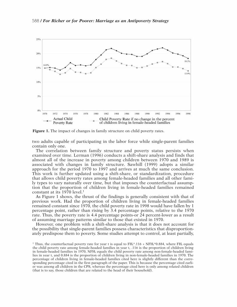
The correlation between family structure and poverty status persists whenexamined over time. Lerman (1996) conducts a shift-share analysis and finds thatalmost all of the increase in poverty among children between 1970 and 1989 isassociated with changes in family structure. Sawhill (1999) adopts a similarapproach for the period 1970 to 1997 and arrives at much the same conclusion.This work is further updated using a shift-share, or standardization, procedurethat allows child poverty rates among female-headed families and all other fami-ly types to vary naturally over time, but that imposes the counterfactual assump-tion that the proportion of children living in female-headed families remainedconstant at its 1970 level.1

As Figure 1 shows, the thrust of the findings is generally consistent with that ofprevious work. Had the proportion of children living in female-headed familiesremained constant since 1970, the child poverty rate in 1998 would have fallen by 1percentage point, rather than rising by 3.4 percentage points, relative to the 1970rate. Thus, the poverty rate is 4.4 percentage points-or 24 percent-lower as a resultof assuming marriage patterns similar to those that existed in 1970.

However, one problem with a shift-share analysis is that it does not account forthe possibility that single-parent families possess characteristics that disproportion-ately predispose them to poverty. Some studies attempt to control, at least partially,

Figure 1. The impact of changes in family structure on child poverty rates.

1 Thus, the counterfactual poverty rate for year t is equal to FHt*.116 + NFHt*0.884, where FHt equalsthe child poverty rate among female-headed families in year t, .116 is the proportion of children livingin female-headed families in 1970, NFHt equals the child poverty rate among non-female-headed fami-lies in year t, and 0.884 is the proportion of children living in non-female-headed families in 1970. Thepercentage of children living in female-headed families cited here is slightly different than the corre-sponding percentage cited in the first paragraph of the paper. This is because the percentage cited earli-er was among all children in the CPS, whereas the percentage cited here is only among related children(that is to say, those children that are related to the head of their household).

For Richer or for Poorer: Marriage as an Antipoverty Strategy / 589

for such characteristics. Cancian and Reed (2000) conduct an analysis that resem-bles the one described above, but they decompose changes in the poverty rate intothose associated with changes in family structure and female labor force behavior.Eggebeen and Lichter (1991) adopt an approach that is similar to Cancian andReed’s, although they conduct separate analyses for black and white families.Gottschalk and Danziger (1993) decompose changes in the child poverty rate intochanges in mothers’ demographic characteristics (race, age, education level, andregion of residence), changes in the proportion of children living in female-headedfamilies, and changes in the size and income of families falling into each joint fam-ily-type/demographic subgroup.

Each of these studies finds that the incidence of single parenthood has a consid-erable impact on the incidence of poverty. Cancian and Reed find that changes infamily structure alone would have led to a poverty rate increase of 3.6 percentagepoints between 1969 and 1998 (the poverty rate actually rose by only nine tenths ofa percentage point over this period). Eggebeen and Lichter’s results suggest that,had there been no changes in family structure between 1960 and 1998, the black

Table 1. Previous findings regarding the effects of family formation on poverty.


child poverty rate in 1998 would have been 28.4 percent rather than 45.6 percent,and the white child poverty rate would have been 11.4 percent rather than 15.4 per-cent. Gottschalk and Danziger find that, all things being equal, increases in femaleheadship between 1968 and 1986 would have led to an increase in the child pover-ty rate of 12.9 percentage points among blacks, and of 3.0 percentage points amongwhites (the black child poverty rate actually declined by four tenths of a percentagepoint over this period, whereas the white child poverty rate increased by 4.8 per-centage points). Table 1 shows summaries of these findings along with briefdescriptions of the analyses that generated them.

From a policy standpoint, this literature does not necessarily imply thatincreases in marriage among single parents would inevitably reduce poverty.There could be differences between currently married men and women and theirunmarried counterparts that these analyses fail to capture. For instance, theremight be unobservable disparities between the earnings potential of married andunmarried adults, or between the work opportunities available to them. If so,poverty is less a function of family formation per se than of unobservable char-acteristics that affect both poverty status and family structure. Such argumentsare consistent with Bane’s (1986) hypothesis that the “feminization” of povertypartially reflects a “reshuffling” of already-poor families across family types, asopposed to the creation of newly-poor families as the result of increases infemale headship. To the extent that this theory is correct, additional marriagemay have less of an ameliorative effect on poverty than the literature reviewedabove would otherwise suggest.

Another well-known thesis is that there are not enough suitable men to allowfor substantial increases in marriage among female-headed families. Wilson andNeckerman (1987) argue that much of the growth in black female headship is theresult of rising male joblessness and its correlate, the reduction in the availablepool of “marriageable men.” The authors create a “male marriageable pool index”(MMPI), which is defined as the ratio of employed men per 100 women of thesame age and race. They show that the increase in black female headship since1970 was accompanied by steep reductions in the MMPI among young and mid-dle-aged nonwhites, and they suggest that the latter trend may have contributedto the former.

However, subsequent research has shown that declines in the employment andearnings of black men can explain only a small proportion—probably no morethan a fifth—of the increase in black female headship (Ellwood and Crane, 1990;Lerman, 1989; Mare and Winship, 1991; McLanahan and Casper, 1995). And inmore recent work, Wilson (1996) acknowledges that emerging evidence relatingto the “marriageable male” theory is mixed. He suggests that cultural norms mayplay a greater role in family formation patterns than was originally thought.Nonetheless, the available evidence indicates that the size of the pool of mar-riageable men has had some consequences for family structure, even if the mag-nitude of this effect is smaller than was initially suggested. Insofar as there is infact a shortage of marriageable males, meaningful increases in marriage withinlow-income minority communities might not be possible, or may only serve tobring men with little or no earnings into families whose incomes are alreadyinsufficient to meet their needs.

Given the likelihood of unobservable differences between married and unmar-ried adults, as well as a possible shortage of marriageable minority men, it is dif-ficult to predict the antipoverty effects of additional marriage using traditionalresearch techniques. For this reason, a microsimulation is conducted to estimate


directly the effect higher marriage rates would have on child poverty. Using 1999census data, new marriages among eligible observations are simulated and fami-ly income and poverty status among these “newly-married” families are recalcu-lated. This approach makes it possible to account explicitly for possible shortagesof marriageable males, and for any unobservable differences between the earn-ings capacity of married and unmarried adults. Lerman (1996) conducts a simi-lar analysis using 1990 census data and finds that increases in marriage wouldconsiderably reduce child poverty. The simulation process builds on Lerman’spioneering work, improves upon it, and extends it in new directions.2

The microsimulation findings suggest that, had the proportion of children livingin female-headed families in 1998 been the same as in 1970, the official 1998 childpoverty rate would have fallen by 3.4 percentage points relative to its actual 1998level. This is a somewhat smaller decline than the 4.4 percentage point drop esti-mated on the basis of the shift-share analysis. Among children involved in simu-lated marriages, however, the poverty rate falls by almost two-thirds. Theseantipoverty effects are greater for black than for white children, lending some sup-port to the theory that there is a lack of marriageable minority males. The findingshold true for a variety of alternative specifications regarding the treatment ofcohabitors in this analysis.

METHODS AND DATA

The marriage microsimulation is performed on data gathered by the Bureau of theCensus during the March 1999 administration of the Current Population Survey(CPS).3 In order to obtain a more accurate sense of the actual level of families’ dis-posable resources, the official CPS measure of income is adjusted to take intoaccount federal tax liability, work-related child care expenses, and receipt of foodstamp benefits and earned income tax credit (EITC) payments.4 All income andpoverty measures used in the microsimulation incorporate these adjustmentsunless otherwise specified.

2 Lerman sorts his male and female samples by age and education level and then merges these sam-ples in order to create matches. He conducts separate matching processes for black and non-Hispanicwhite observations (he deals only with these two racial groups). We use a process that places men andwomen into race, age, and education categories and creates matches only among observations thatmatch on all criteria. After marriages are simulated, Lerman subtracts the mother’s entire welfarebenefit from the new family’s income. We recalculate a range of government benefits—including foodstamps, supplemental security income, cash assistance, and earned income tax credit payments—using a procedure that is somewhat more sophisticated (an appendix describing our benefit-recalcu-lation process is available upon request). And finally, we test the sensitivity of our results to theincreasing prevalence of cohabitation.3 The March CPS is used each year to calculate the official poverty rate. Income characteristics in the1999 survey are for 1998. Family characteristics other than income refer to 1999.4 The tax liability and EITC adjustments are calculated by the authors using variables pertaining tofamily composition, earnings, and adjusted gross income. The food stamp adjustment is based on aCPS estimate of the value of families’ Food stamp benefits. Out-of-pocket child care expenses are cal-culated using a series of parameters estimated by the Census Bureau’s Experimental PovertyMeasures team. These parameters were generated over the course of the team’s analyses of theSurvey of Income and Program Participation. Additional details regarding the methodology used forcalculating child care expenses is available upon request. A thorough discussion of this methodolo-gy can also be found in Short et al. (1999). Some studies also take into account housing costs andmedical expenses. We do not do so here. For excellent summaries of both topics, see Short et al.(1999) and Citro and Michael (1995).


The objective is to set the proportion of children living in female-headed familiesin 1998 equal to the corresponding proportion in 1970. This requires that approxi-mately 9.5 million children living in female-headed families be shifted to the two-parent-family category. To meet this goal, marital matches are assigned to 5.8 mil-lion single mothers.5 These mothers are matched with unrelated males.6 Maritalpartners are allocated using three characteristics as matching criteria: race, age,and level of education. This approach is in keeping with the findings of a numberof studies that show evidence of marital sorting by race, age, and education(Blackwell and Lichter, 2000; Garfinkel, Glei, and McLanahan, 2000; Kalmijn, 1991;Lerman, 1996; Qian and Preston, 1993; Spanier, 1983).7 Observations are dividedinto four race and ethnicity categories (white non-Hispanic, black non-Hispanic,Hispanic, and other), seven age categories (18 to 24, 25 to 29, 30 to 34, 35 to 39, 40to 49, 50 to 64, and 65+), and five education categories (less than high school, highschool graduate, some college, college graduate, and more than college).

Matches are assigned using a method known as “hot-deck allocation.”8 For eachsingle mother participating in the simulation, the hot-deck process searches for anunrelated male falling into the same race, age, and education categories. When such

Table 2. Measures of marital homogamy among existing and simulated marriages.

Among existing Among simulated marriages in the marriages

1999 CPSMean age difference between spouses 3.8 2.5

Mean difference in years ofeducation between spouses 1.7 0.7

Percent marrying within theirown racial/ethnic group* 94.7% 100%

* We assign observations to one of four racial/ethnic categories: white non-Hispanic, black non-Hispanic, Hispanic, and other. Mean differences reflected in this table are calculated as the averageabsolute value of the difference between the ages and years of education of the husband and wife.

5 We impose a constraint that an observation must be at least 18 years of age to participate in a simu-lated marriage. The target number of children is based on a comparison of the proportion of childrenliving in female-headed households in 1970 and 1998. In 1970, 11.6 percent of children lived in female-headed households. In 1998, this percentage was 25.1 percent. To equalize these percentages, we mustshift 25.1 percent –11.6 percent = 13.5 percent of children in 1998 from female-headed to two-parentfamilies. There were 70.8 million children in the United States in 1998; our goal is therefore to shift 70.8million *0.135 = 9.5 million children. The female-headed families participating in the marriage simula-tion contain an average of 1.6 children. We therefore assign matches to 9.5 million ÷ 1.6 = 5.8 millionmothers. The reader should bear in mind that the 1999 CPS actually reflects income characteristics from1998 and family-composition characteristics from 1999. However, for purposes of convenience, we dis-cuss both types of characteristics as though they are for 1998.6 Approximately 18 percent of the single parents in our data are men. To maintain consistency with thespecification of the shift-share analysis, however, we assign marital matches only to single mothers. Wehave conducted sensitivity analyses in which single fathers are included in the matching process. Thisexpanded focus does not substantively affect our results.7 A drawback of our matching process is that it does not take into account the geographic location ofspouses participating in simulated marriages. Thus, we cannot ensure that matches are created betweenmen and women living in the same area.8 This is also the tool used by the Census Bureau to impute missing values for the CPS (Bureau of LaborStatistics, 2000, ch. 9).


an individual is identified, a match is created and both observations are excludedfrom subsequent mate searches. The matching process often identifies multipleobservations that would be appropriate partners for a particular single mother. Insuch instances, a partner is randomly selected from among the qualifying observa-tions. Initially, more suitable matches are created than necessary to meet the targetnumber of simulated marriages. From among the pool of available matches, theappropriate number of marriages is randomly selected. It was easier to find goodmatches for white mothers than for black mothers. Thus, a disproportionate num-ber of the matches created are among white men and women.

Table 2 compares the extent of marital homogamy among the simulated marriagesand existing marriages in the CPS. On all three matching criteria, the simulated cou-ples are more homogamous than existing marital couples. Table 3 shows that, interms of annual earnings, the spouses in simulated marriages are also more alike thanspouses in existing marriages. The annual earnings differential between spouses, bothin nominal terms and as a percentage of the husband’s average earnings, is smalleramong simulated than among existing marriages. Newly matched couples earn about$12,000 less, on average, than existing couples. In addition, the wife’s annual earningsexceed her husband’s more often among simulated than among existing marriages.

The latter finding is largely attributable to the fact that unemployed men areallowed to participate in simulated marriages. To test Wilson and Neckerman’s(1987) “marriageable male” hypothesis, which defines the stock of marriageablemen according to their employment status, a sensitivity test is conducted in whichmen are allowed to participate in the marriage simulation only if they have earn-ings. Another sensitivity test imposes a restriction that marriages can only be cre-ated among couples in which the man’s earnings exceed the woman’s. In bothinstances, even after the constraint is imposed, the hot-deck process creates morewell-matched couples than are necessary to meet the objective.

It could be argued that earnings differentials among many newly matched cou-ples would increase after marriage, since women are less likely to need to work, andsince some studies suggest that men’s earnings tend to increase as a result of mar-riage. For instance, Chun and Lee (2001) and Daniel (1995) find that men enjoy aso-called “marriage wage premium” upon marrying, in which their hourly wageincreases after they marry. These findings are consistent with Becker’s (1981) theo-

Table 3. Annual earnings differentials of spouses in existing and simulated marriages.

Among existing marriages Among simulated marriagesin the 1999 CPS

Average annual earnings of the Husband $36,856 $25,227

Average annual earningsof the Wife $15,908 $15,859

Difference in average annual earnings $20,948 $9,368

Average earnings differentialas a proportion of the husband's earnings 56.8% 37.1%

Proportion of couples in which the wife earns more than the husband 19.3% 30.9%


ry that marriage tends to allow for a more efficient division of household labor,which, in turn, enhances the husband’s labor force productivity.

However, Nakosteen and Zimmer (1987) find that marriage does not, in fact, direct-ly affect men’s wages, and Cornwell and Rupert (1997) suggest that the relationshipbetween marriage and wages can largely be attributed to unobservable characteristicscorrelated with marital status, rather than to the phenomenon of marriage itself. Inaddition, Blackburn and Korenman (1994) find that the size of the marriage premi-um has declined over time. In light of such findings, the authors remain circumspectabout the magnitude and precise causal nature of this relationship, and have there-fore elected not to simulate any earnings changes after marriage.9

After the appropriate number of marriages is selected, the incomes and povertythresholds are re-estimated for all families whose composition changes as a result ofthe simulation. A number of other variables that are affected by changes in familyincome, size, and composition are also recalculated. Specifically, the following arere-estimated: tax liability, work-related child care expenses, and four types of gov-ernment benefits—EITC payments, food stamps, public assistance, and supplemen-tal security income (SSI). Child care expenses, tax liability, and EITC benefits arerecalculated using the process described in footnote 4. The method used to recalcu-late food stamps, public assistance, and SSI benefits is detailed in an appendix thatis available from the authors upon request. After adjusted family income is recalcu-lated, poverty status is reassessed for all families affected by the simulation.10

RESULTS

Table 4 shows that, after the marriage simulation, the unadjusted 1998 child pover-ty rate falls from 18.3 percent to 14.9 percent, which represents a 19.1 percentreduction in the total number of poor children. (Unadjusted poverty rates are cal-culated using the official measure of income, rather than the adjusted measure thattakes into account tax liability, child care expenses, and receipt of government ben-efits.) This reduction is somewhat smaller than the drop from 18.3 percent to 13.9percent elicited by the shift-share analysis. However, it is large enough to reduce thepoverty rate to its 1970 level.

Row 1 of Table 5 shows that, as a result of the microsimulation, the adjusted childpoverty rate falls from 16.9 percent to 13.5 percent, a 20.1 percent reduction.Additional analyses (not shown here) indicate that 26.2 percent of poor white childrenand 16.8 percent of poor black children are lifted out of poverty. The CPS, like manyother surveys, undercounts certain demographic groups—most notably, minority

Table 4. Comparison of the effects of the standardization and microsimulation analyses onunadjusted child poverty.

1970 1998Actual child poverty rate 14.9% 18.3%Standardized to reflect 1970 family composition 14.9% 13.9%Simulated to reflect 1970 family composition 14.9% 14.9%

9 Lerman (1996) does, in fact, simulate earnings changes in some of his analyses; see his paper for a dis-cussion of the possible distributional implications of such a phenomenon.10 We make the simplifying assumption that participants in the microsimulation were not cohabitingbefore getting married. If couples had been cohabiting, the implications of marriage for their familyincome would be different than our results suggest. In the next section, we supplement our initial find-ings with a range of estimates of the sensitivity of our results to alternative cohabitation assumptions.


men (Bureau of Labor Statistics, 2000, ch. 16; Dalaker and Proctor, 2000). This factclouds the interpretation of racial breakdowns of our results. Black single mothers areunderrepresented among marriage simulation participants because there is a lack ofpotential black male partners in some age and education categories. This phenome-non is quite possibly a result of the aforementioned undercount combined with sam-pling error, but it could also be due to the high rates of mortality and incarcerationamong minority men. Among whites, the number of unrelated males exceeds thenumber of single mothers in almost every age and education group. Consequently,whites are overrepresented among the simulated couples and the microsimulation’santipoverty effects are larger for whites than for blacks.

The last five rows of Table 5 focus specifically on children living in families thatparticipated in the marriage simulation. Rows 2 and 3 show that nearly two-thirdsof poor children whose mother participated in a simulated marriage are lifted outof poverty. In addition, the 200 percent poverty gap among families with childrenparticipating in the simulation falls by 47.4 percent. (The 200 percent poverty gapis calculated as the difference between a family’s adjusted income and two times itspoverty threshold; families with adjusted incomes above this amount are assigneda poverty gap value of 0.) Average per capita income among these children increas-es by 43.2 percent. Their mean income-to-needs ratio increases by 57.9 percent.11

The fact that the percentage increase in the income-to-needs ratio exceeds the per-centage increase in per-capita income suggests that these children’s families arebenefiting from the economies of scale that are factored into the estimation of fed-eral poverty thresholds.12

Table 5. Effects of the marriage microsimulation on adjusted poverty and income.*

Pre- Post- Change Percentsimulation simulation change

Among all observations in the CPS Adjusted 1998 child poverty rate 16.9% 13.5% –3.4% –20.1

Among children whose mothers participated in the marriage simulation

Adjusted 1998 child poverty rate 37.8% 13.1% –24.7% –65.4%

Number of poor children 3,491,054 1,207,219 –2,283,835 –65.4%Family poverty gap (200%) $55.5 billion $29.2 billion –$26.3 billion –47.4%Average per capita family income $7,143 $10,232 $3,089 43.2%Average family income-to-needs ratio 1.59 2.51 0.92 57.9%

* Changes shown in this chart are calculated on a net basis; they take into account both increases anddecreases in income and poverty. Average per capita income estimates and average income-to-needs ratioestimates are calculated as weighted averages among all children living in families that participatedirectly in the marriage simulation. The pre-simulation 200% poverty gap is calculated among the sin-gle-parent families participating in the simulation. The post-simulation poverty gap is calculated amongthe two-parent families created as a result of the matching process. Income measures have been adjust-ed to take into account tax liability, out-of-pocket child care expenses, and receipt of Food Stamps andthe Earned Income Tax Credit.

11 The unit of observation for the computation of average per capita income and average income-to-needs ratios is the child, not the family. Families with relatively more children are therefore given rela-tively more weight in these calculations. Both types of averages are calculated using the adjusted meas-ure of family income.12 Some families might benefit more than our analyses imply. Both Citro and Michael (1995) and Ruggles(1990) suggest that official poverty thresholds understate the economies of scale reaped by larger families.


SENSITIVITY TESTS

The authors have not yet accounted for the possibility that members of cohabitingcouples would be affected differently by marriage than other microsimulation par-ticipants. The CPS does not treat cohabitors as members of the family with whomthey are living, even though they are part of the larger household unit. As such, acohabitor’s income is not counted as available to the family he is living with. In prac-tice, however, a cohabitor might pool resources with other members of the extendedhousehold.13 If this were the case, then a single mother who marries her cohabitingboyfriend would effectively experience no change in her economic well-being. Forthis reason, a series of sensitivity tests are conducted to examine the implications ofalternative cohabitation assumptions for our results.

The March CPS includes a survey question that allows the respondent to list her-self as an “unmarried partner” of the householder. Based on responses to this ques-tion, 5.7 percent of the single mothers participating in the simulation were cohab-iting at the time of marriage.14 However, analyses of other data sources suggest thatresponses to the CPS’s survey question may substantially understate the actualextent of cohabitation in the United States (Casper, Cohen, and Simmons, 1999). Assuch, a second cohabitation measure is estimated based on a method Casper,Cohen, and Simmons (1999) developed. Casper and her colleagues modify an exist-ing measure of cohabitation known as POSSLQ (persons of opposite sex sharing liv-ing quarters), which infers cohabitation status based on household composition.

Table 6. Sensitivity of the microsimulation results to alternative cohabitation assumptions.

Pre- Post- Change Percentsimulation simulation change

Adjusted 1998 child poverty rates before cohabitation is taken into account

Initial microsimulation results 16.9% 13.5% –3.4% –20.1%

Adjusted 1998 child poverty rates after cohabitation is taken into account

Using the CPS's direct measure of cohabitation 16.9% 13.7% –3.2% –18.9%

Using the Adjusted POSSLQ measure of cohabitation 16.9% 14.0% –2.9% –17.2%

13 Bauman (1999) suggests that this is true only to a limited extent. He finds that cohabitors are consid-erably less likely than related family members to contribute income toward their household’s needs. Inaddition, one would expect the effects of cohabitation on income sharing to diminish over time, giventhat cohabiting relationships are typically less durable than marriages.14 We also find that a similar proportion of men participating in the marriage simulation had beencohabiting with a single mother before marrying.15 The original POSSLQ measure defines cohabiting households as those in which two unmarried adults ofthe opposite sex are sharing living quarters. Households containing more than two unmarried adults areexcluded under this definition—even if the “third adult” is related to one of the other members of the house-hold (all individuals over the age of fourteen are considered to be adults in this context). Thus, a residencecontaining a mother, her sixteen-year-old son, and her boyfriend would not be considered to be a cohabit-ing household according to the original POSSLQ measure. Casper and her colleagues expand this definitionby allowing households containing more than two adults to be considered as cohabiting households, so longas there are only two unrelated adults in the household, and so long as those adults are of the opposite sex.Thus, the unrelated adults in the three-person household described above would be considered to be cohab-iting under the Adjusted POSSLQ definition, since the third adult (the sixteen-year-old child) is related toone of the other household members. Our thanks to Lynne Casper and Philip Cohen for sharing with us thecomputer code that they developed to identify cohabiting households using this methodology.


Their adjusted POSSLQ uses a broader—and, in the authors’ opinion, more appro-priate—definition of cohabitation than does the original POSSLQ method.15

According to the adjusted POSSLQ definition, 13.5 percent of single mothers par-ticipating in the marriage simulation had been cohabiting at the time of marriage.

The sensitivity of these results is tested using both the direct survey measure andthe adjusted POSSLQ measure of cohabitation. If one assumes that cohabitorsfully share resources, a cohabiting single mother’s family would experience little orno change in its income or poverty status as a result of marriage.16 Therefore, themarriages of any cohabiting women participating in the marriage simulation are“nullify,” thereby eliminating the changes in family income that they otherwisewould have experienced. Then, the effects of the simulation on adjusted childpoverty are re-estimated. Table 6 shows that incorporating the direct survey meas-ure of cohabitation into the analysis reduces the antipoverty effects of the mar-riage simulation by two-tenths of a percentage point. Taking the adjusted POSSLQmeasure into account reduces the simulation’s antipoverty impact by half of a per-centage point. Under either scenario, however, the general thrust of our findingsremains unchanged.17

CONCLUSION

These analyses suggest that policies designed to engender marriage among singleparents could have a considerable effect on child poverty. However, a number ofcaveats are in order. First, this analysis does not take into account the potential forbehavioral shifts brought about by marriage. To the extent that labor force partici-pation were to decline-or fertility were to increase-among mothers participating inthe microsimulation, the results may overstate the poverty-reducing effects of mar-riage. Second, evidence that changes in social policy can have a significant effect onfamily formation patterns is limited, and many remain skeptical about its ability todo so (Ellwood, 2001; Harknett and Gennetian, 2001; Murray, 2001).18 And finally,these analyses take into account only the economic effects of marriage. Ideally, oneshould evaluate a policy based on its ramifications for a broad range of measuresof child welfare, of which economic welfare is only one. Nonetheless, assuming thatone could craft policies with meaningful implications for family formation, thisanalysis suggests that such initiatives could have a large impact on child well-being.The authors gratefully acknowledge the financial support of the Annie E. Casey Foundation.Thanks to Molly Fifer and Sarah Siegel for their important research contributions to thisproject. We would also like to thank Catherine McLoughlin, Shannon Smith, and Sara Belzfor their excellent research and administrative assistance. Thanks also to Bob Lerman, GaryBurtless, Daniel Lichter, Greg Acs, Lynne Casper, Philip Cohen, and three anonymous refer-ees, all of whom provided us with valuable comments and suggestions.

16 Certain income adjustments—including taxes owed and some government benefits—would change ifcohabitors were to marry.17 An alternative means of addressing this issue would be to treat cohabiting couples as though they arealready married. This would require that we recalculate the incomes of those living in cohabiting house-holds by combining the resources of cohabiting couples and their families. Many of these householdswould be lifted out of poverty as a result. This approach would therefore affect the pre- and post-simu-lation poverty levels reported in Table 6. However, our estimates of the percentage-point impact of mar-riage on the poverty rate would remain unaffected. 18 For some evidence that welfare reform may be having an impact on the proportion of children livingin single-mother families, see Acs and Nelson (2001), Bavier (2001), Dupree and Primus (2001), andSawhill (2002).


ADAM THOMAS is a Senior Research Analyst at The Brookings Institution,Washington, DC.ISABEL SAWHILL is a Senior Fellow at The Brookings Institution, Washington, DC.

REFERENCES

Acs, G., & Nelson, S. (2001). Honey, I’m home: changes in living arrangements in the late1990s. Washington, DC: Urban Institute.

Bane, M.J. (1986). Household composition and poverty. In Danziger & Weinberg, eds.,Fighting poverty: what works and what doesn’t (pp. 209-231). Cambridge, MA: HarvardUniversity Press.

Bauman, K. (1999). Shifting family definitions: the effect of cohabitation and other nonfam-ily household relationships on measures of poverty. Demography, 36, 315-325.

Bavier, R. (2001). Recent increases in the share of young children living with married moth-ers. Paper presented at the Brookings Institution, October 15.

Becker, G. (1981). A treatise on the family. Cambridge, MA: Harvard University Press.

Blackburn, M., & Korenman, S. (1994). The declining marital-status earnings differential.Journal of Population Economics, 7, 249-270.

Blackwell, D., & Lichter, D. (2000). Mate selection among married and cohabiting couples.Journal of Family Issues, 21, 275-302.

Bureau of Labor Statistics. (2000). Design and methodology. Current population survey tech-nical paper no. 63. Washington, DC: U.S. Government Printing Office.

Cancian, M., & Reed, D. (2000). Trends in Family Structure and Behavior and the PovertyProblem. Paper prepared for conference on Understanding Poverty in America: Progress andProblems. Madison, WI: Institute for Research on Poverty, University of Wisconsin-Madison.

Casper, L., Cohen, P., & Simmons, T. (1999). How does POSSLQ measure up? Historical esti-mates of cohabitation. U.S. Census Bureau Population Division working paper no. 36.Washington, DC: U.S. Census Bureau.

Chun, H., & Lee, I. (2001). Why do married men earn more: productivity or marriage selec-tion? Economic Inquiry, 39, 307-319.

Citro, C., & Michael, R., eds. (1995). Measuring poverty: a new approach. Washington, DC:National Academy Press.

Cornwell, C., & Rupert, P. (1997). Unobservable individual effects, marriage and the earningsof young men. Economic Inquiry, 35, 285-294.

Dalaker, J., & Proctor, B. (2000). Poverty in the United States: 1999. U.S. Census BureauCurrent population report no. P60-210. Washington, DC: U.S. Government Printing Office.

Daniel, K. (1995). The marriage premium. In Tommasi & Ierulli, eds., The new economics ofhuman behavior (pp. 113-125). Cambridge: Cambridge University Press.

Dupree, A., & Primus, W. (2001). Declining share of children lived with single mothers in thelate 1990s. Washington, DC: Center on Budget and Policy Priorities.

Eggebeen, D., & Lichter, D. (1991). Race, family structure, and changing poverty amongAmerican children. American Sociological Review, 56, 801-817.

Ellwood, D. (2001). The impact of the earned income tax credit and social policy reforms onwork, marriage, and living arrangements. Joint Center for Poverty Research WorkingPaper no. 124. Cambridge, MA: Harvard University.

Ellwood, D., & Crane, J. (1990). Family change among black Americans: what do we know?Journal of Economic Perspectives, 4, 65-84.

Garfinkel, I., Glei, D., & McLanahan, S. (2000). Assortative mating among unmarried par-ents: implications for child support enforcement. Journal of Population Economics.


Gottschalk, P., & Danziger, S. (1993). Family structure, family size, and family income:accounting for changes in the economic well-being of children, 1968-1996. In Danziger &Gottschalk, eds., Uneven tides: rising inequality in America (pp. 167-193). New York:Russell Sage Foundation.

Harknett, K., & Gennetian, L. (2001). How an earnings supplement can affect the maritalbehavior of welfare recipients: evidence from the Canadian Self-Sufficiency Project. SocialResearch and Demonstration Corporation Working Paper.

Kalmijn, M. (1991). Shifting boundaries: trends in religious and educational homogamy.American Sociological Review, 56, 786-800.

Lerman, R. (1989). Employment opportunities of young men and family formation.American Economic Review, 79, 62-66.

Lerman, R. (1996). The impact of the changing U.S. family structure on poverty and incomeinequality. Economica, 63, S119-S139.

Mare, R., & Winship, C. (1991). Socioeconomic change and the decline of marriage for blacksand whites. In Jenks & Peterson, eds., The urban underclass (pp. 175-202). Washington,DC: Brookings Institution Press.

McLanahan, S., & Casper, L. (1995). Growing diversity and inequality in the American fam-ily. In Farley, ed., State of the union, America in the 1990s, vol. 2: Social trends (pp. 1-43).New York: Russell Sage Foundation.

Murray, C. (2001). Family formation. In Blank & Haskins, eds., The new world of welfare (pp.137-168). Washington, DC: Brookings Institution Press.

Nakosteen, R., & Zimmer, M. (1987). Marital status and earnings of young men: a model withendogenous selection. Journal of Human Resources, 22, 248-268.

Qian, Z., & Preston, S. (1983). Changes in American marriage, 1972-1987: availability andforces of attraction by age and education. American Sociological Review, 58, 482-495.

Ruggles, P. (1990). Drawing the line—alternative poverty measures and their implications forpublic policy. Washington, DC: Urban Institute Press.

Sawhill, I. (1999). Families at risk. In Aaron & Reischauer, eds., Setting national priorities:the 2000 elections and beyond (pp. 97-135). Washington, DC: Brookings Institution Press.

Sawhill, I. (2002). The perils of early motherhood. The Public Interest 146:74-84.

Sawhill, I., & Thomas, A. (2001). A hand up for the bottom third: toward a new agenda forlow-income working families. Children’s Roundtable working paper. Washington, DC:Brookings Institution.

Short, K., Garner, T., Johnson, D., & Doyle, P. (1999). Experimental poverty measures: 1990to 1997. U.S. Census Bureau Current population reports, consumer income, P60-205.Washington, DC: Government Printing Office.

Spanier, G. (1983). Married and unmarried cohabitation in the United States: 1980. Journalof Marriage and the Family, 45, 277-288.

U.S. Census Bureau (2001a). Historical poverty table 10: related children in female house-holder families as a proportion of all related children, by poverty status: 1959 to 2000.http://www.census.gov/hhes/poverty/histpov/hstpov10.html.

U.S. Census Bureau (2001b). CH-1: living arrangements of children under 18 years old: 1960to present. http://www.census.gov/population/socdemo/hh-fam/tabCH-1.txt.

Wilson, W.J. (1996). When work disappears: the world of the new urban poor. New York:Alfred A. Knopf Press.

Wilson, W.J., with Neckerman, K. (1987). Poverty and family structure: the widening gapbetween evidence and public policy issues. In Wilson, The truly disadvantaged (pp. 63-92).Chicago: University of Chicago Press.

for richer or for poorer: marriage as an antipoverty strategy

Documents