for review only - university of toronto t-space review only non-equilibrium phase and entanglement...

For Review O

nly

Non-equilibrium phase and entanglement entropy in $2D$ holographic superconductors via Gauge-String duality

Journal: Canadian Journal of Physics

Manuscript ID cjp-2016-0338

Manuscript Type: Article

Date Submitted by the Author: 16-May-2016

Complete List of Authors: Mazhari, Najme Al Sadat; Eurasian Nat. U., Momeni, Davood; Eurasian Nat. U., Astana, Raza, Muhammad; COMSATS Institute of Science and Technology, Computer Science Gholizade, Hossein; Tampere University Myrzakulov, R.; LN Gumilev Eurasian National University

Keyword: Gauge/gravity duality, entanglement entropy, information metric, holographic superconductors, numerical computations

https://mc06.manuscriptcentral.com/cjp-pubs

Canadian Journal of Physics

For Review O

nly

Non-equilibrium phase and entanglement entropy in 2D

holographic superconductors via Gauge-String duality

Najmeh Al Sadat Mazhari,∗ Davood Momeni,†,‡ and Ratbay Myrzakulov§

Eurasian International Center for Theoretical Physics

and Department of General & Theoretical Physics,

Eurasian National University, Astana 010008, Kazakhstan

Hosein Gholizade¶

Department of Physics, Tampere University of

Technology P.O.Box 692, FI-33101 Tampere, Finland

Muhammad Raza∗∗

Department of Mathematics, COMSATS Institute of

Information Technology, Sahiwal 57000, Pakistan

(Dated: July 25, 2016)

† Corresponding author

1

Page 1 of 29



For Review O

nly

Abstract

An alternative method of developing the theory of non-equilibrium two dimensional holographic

superconductor is to start from the definition of a time dependent AdS3 background. As originally

proposed, many of these formulae were cast in exponential form, but the adoption of the numeric

method of expression throughout the bulk serves to show more clearly the relationship between

the various parameters. The time dependence behavior of the scalar condensation and Maxwell

fields are fitted numerically. A usual value for Maxwell field on AdS horizon is exp(−bt), and

the exponential log ratio is therefore 10−8s−1. The coefficient b of the time in the exponential

term exp(−bt) can be interpreted as a tool to measure the degree of dynamical instability; its

reciprocal 1b is the time in which the disturbance is multiplied in the ratio. A discussion of some

of the exponential formulae is given by the scalar field ψ(z, t) near the AdS boundary. It might

be possible that a long interval would elapse the system which tends to the equilibrium state

when the normal mass and conformal dimensions emerged. A somewhat curious calculation has

been made, to illustrate the holographic entanglement entropy for this system. The foundation of

all this calculation is, of course, a knowledge of multiple (connected and disconnected) extremal

surfaces. There are several cases in which exact and approximate solutions are jointly used; a

variable numerical quantity is represented by a graph, and the principles of approximation are

then applied to determine related numerical quantities. In the case of the disconnected phase with

a finite extremal are, we find a discontinuity in the first derivative of the entanglement entropy as

the conserved charge J is increased.

PACS numbers:

Keywords: Entanglement entropy, gauge-gravity duality,AdS/CFT, phase transitions

∗Electronic address: [email protected]‡Electronic address: [email protected]§Electronic address: [email protected]¶Electronic address: [email protected]∗∗Electronic address: [email protected]

2

Page 2 of 29



For Review O

nly

I. INTRODUCTION

Statistical systems out of the equilibrium have been studied by non-equilibrium statistical

mechanics. Recently inspired by the string theory, using a gauge-gravity duality, such non-

equilibrium physics are revisited by holography[1–27]. By holographic principle we mean a

set up in which the physics of the gauge fields of the strongly coupled system can be extracted

from the asymptotic behavior of the certain fields on the AdS boundary of gravitational bulk

[28]. Among all possibilities to consider bulk-boundary duality, lower dimensional models

are very interesting because of their simplicities and analytical capabilities for investigations

[29]-[36].

As an attempt to study non-equilibrium systems using AdS/CFT (gauge-string dual-

ity),in reference [39], the authors proposed a periodic driving model to confine themselves

to discussing the holographic superconductor and realistic-matter of it, indicating its rela-

tion to the varying chemical potential, and explaining the methods by which systems reach

their condensation. In this connexion we may note that the equilibrium state is reached at

enough long times t → ∞. Some critics propose to substitute for” dual chemical potential

” µ the expression of ρ(t) in a such manner that when t → ∞, ρ(t) → ρ. The method

of attending the equilibrium varies in detail from state to state, but that most usual is for

the dual parameters ρ, µ to propose time depending, often by a prescribed time dependent

form, and for these situations, the equations of the motion to be solved on by the numerical

methods. Besides the works already mentioned, [48], [49], of which they may indicate the

following: considerations time dependent scalar and Maxwell fields; solving equations of

the motion by numerical methods to find behavior of the fields near the AdS horizon to

read the expectation values of the dual operators as functions of time. In this article we

propose the same lower dimensional model, therefore to confine ourselves to discussing the

character and subject-matter of the holographic superconductors, indicating its relation to

AdS3/CFT2, and explaining the methods by which systems reach their equilibrium states,

we don’t assume any prescribed from for {ρ(t), µ(t)}. A numerical algorithm written to pro-

pose a substitute for the system out of the equilibrium is said to have fields ψ(z, t), Aµ(z, t).

As long as they were time evolving together or disrupting the background, what difference

did a small inhomogeneous field Ax(z, t) makes the system out of the equilibrium. There’s a

difference between this work and having the condensation with time dependent prescribed

3

Page 3 of 29



For Review O

nly

form for dual parameters. The superconducting systems need an element to protect them

from these out of the equilibrium fluctuations, not to mention the demons. In our arti-

cle we stabilize the system using the inhomogeneous component of the field Ax(z, t). It is

commonly said that this is the difference between the equilibrium and the inequilibrium

systems. The plan of this paper is as the following: In Sec. (II), we introduce the basic set

up for such time dependence holographic superconductors. Equations of motion and dual

AdS geometry is proposed. A gauge fixing is used to reduce the number degree of freedoms

of the system. In Sec. (III), normal phase portrait is studied. In this section the system of

the equations is simplified as much as we can. In Sec. (IV), we’ll study numerical solutions

for phases of system. Time dependence forms of the fields are investigated near the AdS

boundary. In Sec. (V), we compute holographic entanglement entropy. We’ll show that

how we are able to calculate extremal surfaces in a time dependence background of bulk.

We compute holographic entanglement entropy for connected and disconnected surfaces . In

disconnected phase we calculate holographic entanglement for two limits of the conserved

charge J . We summarize in Sec. (VI).

II. FAR-FROM-EQUILIBRIUM MODEL FOR 2D HOLOGRAPHIC SUPERCON-

DUCTORS

Among the models of holographic superconductors it was undoubtedly [50], whose con-

tributed most to the development of AdS/CFT based superconductors, and to its unfailing

faith in their ultimate realization must be ascribed the completion of the first successful

holographic model for strongly coupled system. At the same time the bulk as a developed

whole is regarded as an static and asymptotically AdS spacetime which is permeated with

the AdS/CFT, and so we may say that the gravity bulk is a self-realization of the boundary

world. The wellknown form of the AdS3 spacetime were already embedding into the 4D flat

spacetime R2,2 with the following flat metric:

g = −(

dX21 + dX2

2

)

+(

dX23 + dX2

4

)

. (1)

We’ll use a set of the embedding coordinates(

t, ρ, θ)

for all of the hyperboloids in this flat

spacetime [37, 38]:

4

Page 4 of 29



For Review O

nly

X1 = l cosh ρ sin t, (2)

X2 = l cosh ρ cos t, (3)

X3 = l sinh ρ sin θ, (4)

X4 = l sinh ρ cos θ (5)

Using this set of the coordinates, and by speciefying an AdS radius l2 = − 1Λwe obtain the

universal covering of the AdS3 spacetime in the following static form:

ds2 = l2(

− cosh2 ρdt2 + dρ2 + sinh2 ρdθ2)

. (6)

The domain ρ = 0, represent the the AdS boundary of the AdS metric. For our forthcoming

desires to investigate the system out of the equilibrium, we need a non-static time dependent

version of this metric. It can be written in the infalling Eddington coordinates as

ds2 =l2

z2[−f(z)dt2 − 2dtdz + dx2], (7)

where the blackening factor is given by f(z) = 1− ( zzh)2 with z = zh the position of horizon

and z = 0 the AdS boundary.

The formulation of 2D charged holographic superconductor with a global U(1) symmetry

was due to [50]. Let us start with the following bulk action in which gravity is coupled to

an Abelian gauge field A in the presence of a generally massive scalar field Ψ with charge q

and mass m, i.e.,

S =

∫

Md3x

√−g[ 1

2κ2

(

R +2

l2

)

r + (−1

4FabF

ab − |DΨ|2 −m2|Ψ|2)], (8)

here l is the AdS radius, andD = ∇−iA with∇ ≡ ∂µ , Maxwell tensor is Fµν = ∂µAν−∂νAµ.We’ll work in the probe limit, which can be achieved by taking the limit κ2 = 0. The

equations of motion:

DµDµΨ−m2Ψ = 0, (9)

∇µFµν = i[Ψ∗DνΨ−Ψ(DνΨ)∗]. (10)

We define the CFT temperature as the Hawking temperature of the horizon by the following

formula:

T =1

2πzh. (11)

5

Page 5 of 29



For Review O

nly

The earliest formulation of the subject, due to [50], assumed that when we evaluate the

Abelian gauge field A at the AdS boundary, it can be considered as a source with con-

served current J . This later conserved current is associated to a global U(1) symmetry.

Furthermore, the near AdS boundary z ∼ 0 data of the scalar field Ψ provides a physical

sources for the scalar operator O. This relevant operator has the conformal scaling dimen-

sion ∆± = 1±√1 +m2l2. In this article we study the case of m2l2 = 0,∆ = ∆+ = 2

With knowledge then of the conformal dimension of scalar field of the conformal operators

involved in boundary conformal action, we can at once calculate the asymptotic solution of

A and Ψ near the AdS boundary, by placing for each compound in the field equations its

asymptotic metric, i.e f(z) ∼ 0.

From these numbers we can, by help of the AdS/CFT dictionary, calculate the vacuum

expectation value (VEV) of the corresponding boundary quantum field theory operators. In

our case, these VEV quantities are 〈J〉 and 〈O〉. Basically we can compute these quantities

using the following variations of the effective and renormalized action δSren :

〈Jν〉 = δSrenδaν

= limz→0

√−gq2

F zν , (12)

〈O〉 = δSrenδφ

= limz→0

[z√−glq2

(DzΨ)∗ − z√−γl2q2

Ψ∗], (13)

where Sren is the renormalized action :

Sren = S − 1

lq2

∫

B

√−γ|Ψ|2, (14)

and by dot we mean derivative with respect to the time coordinate t. In our work for

simplicity, we set l = 1, q = 1, and zh = 1. We can calculate the expectation value

of condensation of operators from its asymptotic fields for any substance lived in a given

bulk, from a knowledge of the temperature of boundary, by means of an application of the

well-known thermodynamical process.

Now we are fixing the fields as Ψ = Ψ(x, z, t),A = At(x, z, t)dt + Ax(x, z, t)dx. By the

fixing of this gauge field A, the task of the time driven superconductor was considerably

simplified. The corresponding equations of motion are written in an explicit form:

2∂t∂zψ +2

z2fψ − f ′

zψ − f ′∂zψ − f∂2zψ − i

(

∂zAtψ + 2At∂zψ)

− ∂2xψ + i(

∂xAxψ + 2Ax∂xψ)

+A2xψ − 2

z2ψ = 0 (15)

6

Page 6 of 29



For Review O

nly

for the Klein-Gordon equation with Ψ = zψ and the following partial differential equations

for gauge fields:

∂2zAt − ∂z∂xAx = i(ψ∗∂zψ − ψ∂zψ∗), (16)

∂t∂zAt + ∂t∂xAx − ∂2xAt − f∂z∂xAx = −i(ψ∗∂tψ − ψ∂tψ∗)− 2Atψ

∗ψ (17)

+if(ψ∗∂zψ − ψ∂zψ∗),

∂z∂xAt + f∂2zAx + f ′∂zAx − 2∂t∂zAx = i(ψ∗∂xψ − ψ∂xψ∗) + 2Axψ

∗ψ (18)

By prime here we mean the differentiation of the fields with respect to z. We suppose that

the Maxwell gauge fields satisfy the following ansatz:

∂xAt = ∂xAx = ∂xψ = 0. (19)

Thus by equation (19), the equations of motion are expressed by :

2∂t∂zψ +2

z2fψ − f ′

zψ − f ′∂zψ − f∂2zψ − i∂zAtψ − 2iAt∂zψ + A2

xψ − 2

z2ψ = 0, (20)

∂2zAt = i(ψ∗∂zψ − ψ∂zψ∗), (21)

∂t∂zAt = −i(ψ∗∂tψ − ψ∂tψ∗)− 2Atψ

∗ψ + if(ψ∗∂zψ − ψ∂zψ∗), (22)

f∂2zAx + f ′∂zAx − 2∂t∂zAx = 2Axψ∗ψ. (23)

The preceding investigation for (20-23) is based upon the assumption that in passing from

one section of the spacetime to another the homogeneity of the spacetime in the x direction

does not change.

III. PHASE TRANSITION

The main goal of this paper is to study such solutions of system (20-23) which they can

describe superconductor phase. Before the condensation is started, the system is prepared

in the normal phase in which the characteristic temperature of the system T > Tc, where

Tc denotes a specific critical temperature. We suppose that the system is prepared in the

following normal (non superconductor) state:

Ax = ∂tψ = ∂tAt = 0, (24)

7

Page 7 of 29



For Review O

nly

If we apply this assumption to the field equations (20-23), we see that the normal phases is

static solution to the following equation of motion

∂t∂zAt = ∂2zzAt = 0 (25)

Whose solution is given by the following:

ψ = 0, At = µ(1− z). (26)

here by µ we denote the dual chemical potential of the boundary system. To investigate

system in the critical phase T < Tc and when the system enters a phase transition region

from normal to superconductor phase, we need to gauge fixing as ψ = ψ∗. With this gauge

fixing we must solve the following system of partial differential equations (PDEs):

2∂t∂zψ +2

z2fψ − f ′

zψ − f ′∂zψ − f∂2zψ − i∂zAtψ − 2iAt∂zψ + A2

xψ − 2

z2ψ = 0, (27)

∂2zAt = 0, (28)

∂t∂zAt + 2Atψ2 = 0 (29)

f∂2zAx + f ′∂zAx − 2∂t∂zAx − 2Axψ2 = 0. (30)

here ψ = ψ(z, t), At = At(z, t), Ax = Ax(z, t).

IV. NUMERICAL SOLUTIONS

The ultimate value of numerical solutions must depend on the boundary conditions on

which they are based. The value of the gauge field , for instance, is the result of many

factors, some inherent, some due to boundary conditions, and until these have been sifted

out, numerical methods of harmonics or of correlation can have no more than an empirical

value. The appropriate boundary condition near the AdS horizon z = 0 can be written as

the following:

At(0, t) = 0, ψ(0, t) = 〈O+(t)〉z2. (31)

In the vicinity of the horizon z ≃ 1, the appropriate set of BCs are given by the following:

∂zAt = −ρ(t), ψ(z = 1, t) = Σ∞n=1ψ

(n)(z = 1, t)(1− z)n. (32)

Such a hypothetical simplicity is the necessary step for solving the system of PDEs given

in (27-30). Then by solving these equations, regarding the four elements ψ = ψ(z, t), At =

8

Page 8 of 29



For Review O

nly

At(z, t), Ax = Ax(z, t) as unknown quantities, the values of the l{〈O+(t)〉, ψ(n)(z = 1, t)}may be computed. we find that, eliminating (28), the resultant is a homogeneous function

of z of degree 1;

At(z, t) = µ(t)− ρ(t)z (33)

differentiating ∂z of (29) and solving for ψ(z, t) we obtain the scalar field profile;

ψ(z, t) =

√

g(t)

µ(t)− ρ(t)z(34)

if values of g(t), µ(t), ρ(t) , given by any solution, be substituted in each of the two

equations, they will possess a common factor which gives a value of Ax(z, t) , yields a

system of values which satisfies both equations:

[

f∂2z + f ′∂z − 2∂t∂z − 2( g(t)

µ(t)− ρ(t)z

)2]

Ax(z, t) = 0 (35)

and we can solve (27,35). When t→ ∞ the system tends to the equilibrium superconductor

phase. Accordingly the graph of (1) for ψ(z,t)1−z , time evolution of the factor g(t) in (34) is

exponentially decreasing function of time. We assumed that the values of chemical potential

µ and charge density ρ, at each point, was slightly modified, from the equilibrium forms

belonging to a uniform µ ∼ ρ, by the time dependent factor g(t) in the (34). The rate of

diminution of amplitude 〈O+(t)〉 expressed by the coefficient g(t) in the (34) is decreasing

by time. The coefficient b of the time in the exponential term ψ(z,t)1−z ∼ g(t) can be used

to measure the degree of dynamical (in)stability; its reciprocal 1bis the time in which the

disturbance is multiplied in the ratio i. e. τ ∼ 108.

As numerical results indicate, after long time the Ax tends to zero (cf. figure (2)). There-

fore, we can ignore the effects of Ax in the equations and solve the equations of motion. The

analytical expression for the Ax (35) in the latter case involves exponential terms, one of

which decreases rapidly, being equally multiplied in equal times:

Ax (z, t) = F2 (t)−1

2F1

(

2 tanh−1 (z) + t)

(36)

When t → ∞ and near the AdS boundary point, we should satisfy an auxiliary condition

F2 (t)− 12F1 (t) |t→∞ = 0.

9

Page 9 of 29



For Review O

nly

Within this approximation, the result for g(t) is:

g(t) ∼ exp (−t)

Near zh we can analyse the numerical result without setting the Ax = 0. The figure (1)

shows that the form of g(t) near the AdS boundary z = 0.

FIG. 1: ψ(z,t)1−z near AdS boundary point.

The numerical non-linear fitting results for g(t) confirm analytical results:

g(t) = a exp(−bt), (37)

a = 1.10517± 1.95684× 10−8, (38)

b = 1.0± 2.37993× 10−8, (39)

The coefficient a of this function g(t) is equivalent to 〈O+(t)〉, t ≫ τ . The coefficient of

〈O+(t)〉| is a variable quantity depending upon the temperature T of thesystem given in (11)

, but is usually taken to be√

1− TTc

is the fundamental equation between the condensation

and temperature, however the lower order terms may be applied which all vanishes at critical

point T = Tc.

Perhaps the best data for a comparison are those afforded by the computing fitting

residuals for g(t) at different times. Figure (3) shows the fitting residuals for g(t) near AdS

boundary.

Then by solving equation (35), regarding the boundary conditions , the value of the

Ax(z, t) may be computed in Fig.(4). From t = 0 to t ∼ 5 we see a symmetric pattern which

10

Page 10 of 29



For Review O

nlyFIG. 2: Ax(t) near AdS boundary point.

FIG. 3: Fitting residuals near z ∼ 0 for g(t).

will be copied in the next interval times. On Fig. (4) , in the vicinity z = 0, are the remains

of an decreasing exponential factor g(t), said to have been raised by ψ(z, t) in (35). For time

interval t ∈ [ti, tf ],it shows that Ax(z, t) is a monotonic-constant function.

We found a temporary numeric solution to (27), and we plotted the ψ(z, t) around the

(t, z) in Fig.(5). An exponential decreasing form is observed. Furthermore, we observe a

discontinuity in ψ(0, t) near critical point Tc = 0.01 at time scale t ∼ 7. For time intervals

0 < t < 7, 7 < t < 10,it shows that ψ(z, t) is a monotonic-decreasing function.

V. CALCULATION OF HOLOGRAPHIC ENTANGLEMENT ENTROPY

The holographic entanglement entropy (HEE) of a quantum system in boundary is defined

as the entropy of a region of space A and its complement on the minimal surfaces in AdSd+1

using gauge-gravity duality [51]-[53]:

SA ≡ SHEE =Area(γA)

4Gd+1

. (40)

11

Page 11 of 29



For Review O

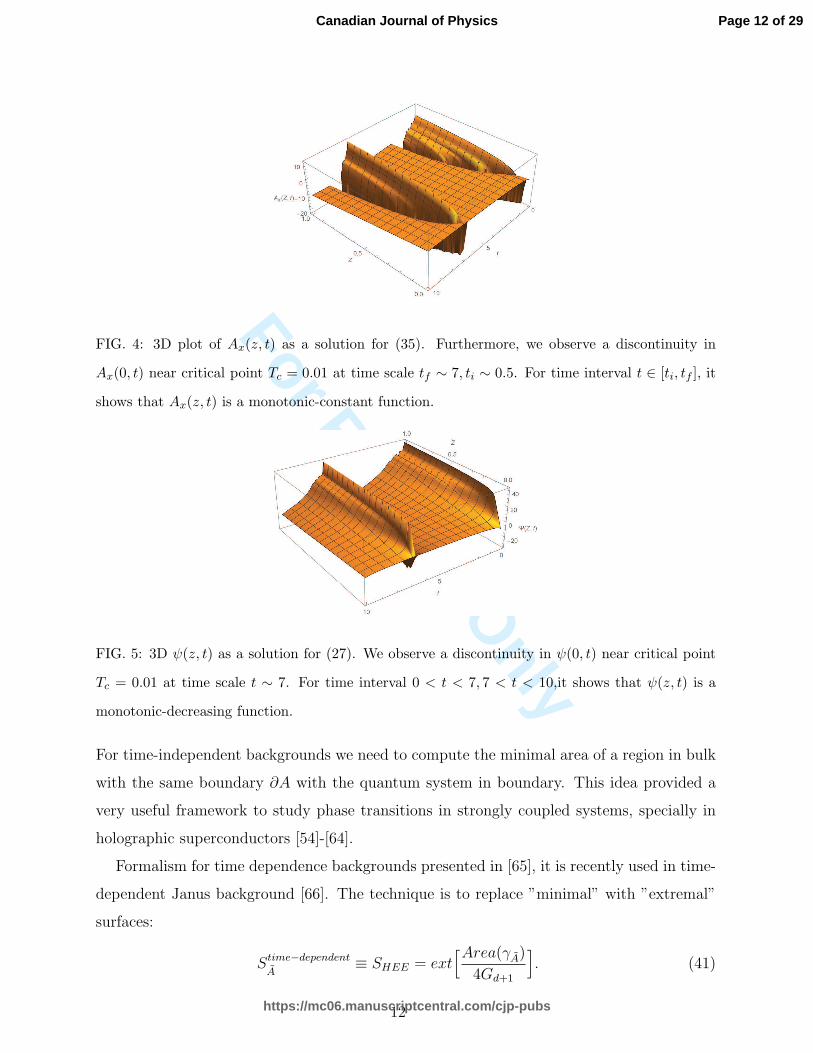
nlyFIG. 4: 3D plot of Ax(z, t) as a solution for (35). Furthermore, we observe a discontinuity in

Ax(0, t) near critical point Tc = 0.01 at time scale tf ∼ 7, ti ∼ 0.5. For time interval t ∈ [ti, tf ], it

shows that Ax(z, t) is a monotonic-constant function.

FIG. 5: 3D ψ(z, t) as a solution for (27). We observe a discontinuity in ψ(0, t) near critical point

Tc = 0.01 at time scale t ∼ 7. For time interval 0 < t < 7, 7 < t < 10,it shows that ψ(z, t) is a

monotonic-decreasing function.

For time-independent backgrounds we need to compute the minimal area of a region in bulk

with the same boundary ∂A with the quantum system in boundary. This idea provided a

very useful framework to study phase transitions in strongly coupled systems, specially in

holographic superconductors [54]-[64].

Formalism for time dependence backgrounds presented in [65], it is recently used in time-

dependent Janus background [66]. The technique is to replace ”minimal” with ”extremal”

surfaces:

Stime−dependentA

≡ SHEE = ext[Area(γA)

4Gd+1

]

. (41)

12

Page 12 of 29



For Review O

nly

In case of multiple extremal surfaces, we should select the extremal surface with the minimum

area included in them.

In applying gauge-string techniques, we use another time coordinate y = t + 2 tanh−1 z

in (7), because the metric on AdS boundary becomes flat which is essential for CFT. The

new appropriate form of metric is given by the following:

ds2 =l2

tanh2(

t−y2

)

[

dx2 − cosh−2(t− y

2

)

dtdy]

. (42)

In this coordinate y, the black hole horizon z = 1 corresponds to y = ∞. Furthermore,

the conformal (AdS) boundary z = 0 is located at the sheet y − t = 0. So, the metric on

conformal boundary is manifested as flat one ds2 ∼ dx2 − dt2.

To compute the extremal surfaces, we should select an appropriate setup with the sub-

system A = {(±y∞, t∞, x)| − x∞ ≤ x ≤ x∞} in the bulk geometry (42). Basically we

have two types of the extremal surface which are different from topologies. These types of

extremal surfaces are defined by connected phase and disconnected phase. The functional

which should be extremized is:

A[t(y), x(y)] = l

∫ y∞

−y∞

dy

tanh(

t−y2

)

√

−t cosh−2(t− y

2

)

+ x2. (43)

here dot denotes the time derivative ddy. The problem is reduced to solve the Euler-Lagrange

(EL) equation(s).

A. Extremal areas in connected phase

For connected surfaces, the surfaces are defined at x = ±x∞, so the functional reduces

to the following form:

A[t(y)]

l=

∫ y∞

−y∞

dy

sinh(

t−y2

)

√

−t. (44)

There is no conserved quantity associated to the coordinate t. We should find the solution

of the following EL equation in which we introduced a new function u(y) = t(y)−y2

:

d2u(y)

dy2= coth(u(y))(1 +

du(y)

dy)(1 + 2

du(y)

dy) (45)

13

Page 13 of 29



For Review O

nly

This differential equation has the following first integral solution:

(1 + u)√

−(1 + 2u) = c sinh u. (46)

This expression gives the unique exact solution of the equations of motion (45).

We can compute explicitly the total area of the connected extremal surface by the fol-

lowing functional:

A[t(y)]

l=

∫ y∞

−y∞

dy

sinh(

u(y)2

)

√

−(1 + 2u). (47)

Using equation(46) we can rewrite the equation(47) as:

A[t(y)]

l=

∫ u(y∞)

u(−y∞)

cosh(u2)

(ξ(u) + 1)ξ(u)du, ξ(u) =

1

6(δ +

1

δ− 5)

here δ =3

√

−27c2 cosh(2u) + 3√6√

c2 sinh2(u)(27c2 cosh(2u)− 27c2 − 2) + 27c2 + 1.

We should notice that we take the real solution of equation (46). Expanding A[t(y)]l

in

powers of c, we have:

A

l=

∫ u(y∞)

u(−y∞)

du(

− 196608c10(sinh11(u)csch(u

2))− 9728c8(sinh9(u)csch(

u

2))

−512c6(sinh7(u)csch(u

2))− 64c4(sinh4(u) cosh(

u

2))− 4 cosh(

u

2))

c=0.01

c=0.02

c=0.03

2 4 6 8 10y

-5

-4

-3

-2

-1

u(y )

FIG. 6: Plot of the solution u(y) as a function of y for different values of c = 0.01, 0.02, 0.03.

In figure (6) we numerically constructed u(y) as a function of y for different values of

c = 0.01, 0.02, 0.03. When y is increasing, u(y) in decreasing up to a local minima, after

14

Page 14 of 29



For Review O

nlyFIG. 7: Plot of the surface A

l versus u(y∞) and c. When y is increasing, u(y) in decreasing up to a

local minima, after that it is increasing by a roughly slope. The minima is located at the turning

point. If we’re increasing c, the local minima is shifted to the right. It can be interpreted as a shift

in the horizon.

that it is increasing by a roughly slope. The minima is located at the turning point. If we’re

increasing c, the local minima is shifted to the right. It can be interpreted as a shift in the

horizon.

In figure (7) we plot regularized HEE per length l as a function of the {u(y∞), c}. It showsthat A

lis a monotonic-increasing function. It always increasing or remaining constant,

and never decreasing. It produces a regular phase of matter for T > Tc or equivalently

for u(y∞) � 15.5. Regular attendance at these non superconducting phase has proved

numerically. Boundary conditions and regular tiny parameter c will help to keep normal

phase for longer. Normal phase increasing the entropy Al, increases the hardenability of

superconductivity.

B. Extremal areas in disconnected phase

In disconnected phase, we should compute the extremal area of the disconnected surfaces

as a function of boundary coordinates (t∞, x∞). We solve the EL equations for t(y) and

x(y) for general functional (43). The associated Noether charge for x is given by J ≡∂∂x

(

A[t(y),x(y)]l

)

. This conserved charge J plays a crucial role in our forthconing results.

If we solve it for x and substitute the result in (43) we obtain:

A[u(y)] = l

∫ y∞

−y∞

dy√

−(1 + 2u)

sinh u(y)√

1− 4J2 tanh2 u(y). (48)

15

Page 15 of 29



For Review O

nly

TABLE I: Coefficents hi(u, J) in (50) .

i hi(u, J)

0 − 1cosh6( 1

2u)

1 24 tanh3(12u) ln(

tanh2( 12u)+4J tanh( 1

2u)+1

− tanh2( 12u)+4J tanh( 1

2u)−1

)

24(1+tanh4( 1

2u)−10 tanh2( 1

2u))

cosh2( 12u)

3 4h1(u, J)

4192 tanh2( 1

2u)

cosh2( 12u)

5 −16h1(u, J)

The returning point location u∗ ≡ (y∗, t∗) is the one which x → ∞. So, J = 12 tanhu∗

. The

EL equation for u(y) in (48) is given by:

u =(1 + 2u)(u2 − 2u− 1)((4J2 − 1) cosh4 u− 4J2)

(1 + u) sinh(2u)(

2J2 sinh2 u− cosh2 u2

) . (49)

This differential equation has a unique first integral solution:

ln√

−(1 + 2u)(u2 − 2u− 1) =Σ5i=0hi(u, J)J

i

12 tanh3 u, (50)

whose general solution is given by the following list of functions:

Equation (50) has three solutions for u. We can summarize the solutions (u− 12) as:

u− 1

2=

ζ

6 3√2+

11

22/3ζ−

(

1− i√3)

ζ

12 3√2

− 11(

1 + i√3)

2 22/3ζ−

(

1 + i√3)

ζ

12 3√2

− 11(

1− i√3)

2 22/3ζ

here

θ =

∑5i=0 hiJ

i

12 tan3(u), ζ =

3

√

√

(378− 108e2θ)2 − 143748− 108e2θ + 378 (51)

We select the first (real) solution for u. We can investigate some limits of extremal surface

areas in disconnected phase:

16

Page 16 of 29



For Review O

nly

1. Near J = 12

The case J = 12is easy to check that the only possible solution for (49) is given by u = u0.

If we compute (48) for this solution, we obtain:

A

l= 2

√

−(1 + 2u0)y∞ (52)

If system evolves in the vicinity of J = 12, a numerical computation shows that A

lis a

monotonic-decreasing function. Near Jc ≈ 0.58+−0.02 we can simplify u = T1 + T2(J − 0.5)

where Ti are functions of u. The expressions Ti are quite lengthy, thus we only record the

results here . It always decreasing. It produces a regular phase of matter for J > Jc. Regular

attendance at these non superconducting phase has proved numerically.

0.55 0.60 0.65 0.70J

-0.25

-0.20

-0.15

-0.10

-0.05

A

l

FIG. 8: Al as a function of J near 1

2 . If system evoles in the vicinity of J = 12 , a numerical

computation shows that Al is a monotonic-decreasing function. It always decreasing. It produces

a regular phase of matter for J > Jc. Regular attendance at these non superconducting phase has

proved numerically.

Formula (52) shows a linearly-dependece expression of reduced HEE (41) as a function

total length y∞. The simple physical reason backs to the emergence of new extra degrees of

freedom in small values of belt length (small sizes). The HEE given in (41) can dominate

on y∞ because in this limit, the main contribution (41) comes from the region u ∼ u∗ ∼ u+.

We can explain it more using the first law of thermodynamic for entanglement entropy. It is

known so far that the HEE is treated like a conventional entropy. So, it naturally obeys the

first law of thermodynamic [67],[68]. Let us to consider y∞ as the length scale of the system.

Thus, the expression dSdy∞

is proportional to the entangled pressure PE = TEdSdy∞

at fixed

temperature in the case of µµc> 1. A constant slope dS

dy∞defines a uniform entangled pressure

17

Page 17 of 29



For Review O

nly

PE. Using the Maxwell’s equations in thermodynamic, we know that(

dSdy∞

)

T=

(

dPdT

)

y∞.

Consequently, if we keep the T fixed, we gain a uniform entropy gradient of HEE(

dSdy∞

)

.

This is equivalent to a uniform gradient of pressure(

dPdT

)

(in fixed belt length). In this case,

we see an emergent constant entropic force [67]. Another simple elementary physical reason

is that S must be an extensive function of characteristic size(length) of the entangled system,

namely y∞. From statistical mechanics we know that if we make the size of the entangled

system larger, here y∞ → ky∞, as a vital fact, the HEE S must also increases. So, HEE S

must be a homogenous function of size. In our case, S is found to be homogenous of first

order, i.e. S(ky∞) = kS(y∞). We conclude that the S ∼ y∞ changes linearly with y∞.

2. Exceeding a normal or reasonable limit: J → ∞

The following area functional is the approximate integral form of the (48): When the

conserved charge J passes through J = 12at a magnitude of several orders, the functional is

given by the following:

A

l≍ 1

2J

∫ u(y∞)

u(−y∞)

du(y)cosh u(y)

sinh2 u(y)

√

1 + 2u(y)

u(y)(53)

We plot the integrand (In) of (53) in figure (9).

-1.0 -0.5 0.5 1.0

10

20

30

40

50

FIG. 9: Plot of integrand (In) of the integral (53) as a function of u(y∞). If u(y∞) → 0, the

integrand is expressed as a singular function In :∼ 0.726543u(y∞)2

− 0.318884− 0.960626u(y∞)2 .

It should be noted that the solution for (49) is, as a rule, only estimates, but in most

instances it probably approximates closely to accuracy. This solution is given by

u±(y) ≡ v + 1±√v2 + 3v + 2, v = e4 sinh

2 u(y) (54)

18

Page 18 of 29



For Review O

nly

This latter functional included the complex integral calculus, the calculus of improper

integrals, the theory of residues and the Cauchy principal value should be found. Because

v > 1, so u−(y) < 0, u+(y) > 0. We choose the u+(y) branch of the solutions to avoid

a negative area functional. The method for determining exact value of the integral (53)

is far in advance of this work, and is identical in principle with the methods of residuals.

If u(y∞) → ∞, then the Cauchy principal value (P.V) of (53) is given by the following

expression:

2JA

l= P.V {

∫ ∞

−∞In(u(y))du(y)} = lim

u(y∞)→∞

∫ u(y∞)

−u(y∞)

In(u(y))du(y) (55)

=

∮

half

In(u(z))dz − limǫ→0

∫ ǫ

−ǫIn(x)du(x)−

∫

CR

In(x)dx− Σ∞n=12πiRes

(

In(u(z)))

u=un

here un = sinh−1(

√π(2n+1)

2e

iπ4

)

and Res(

In(u))

u=un= limu→un(u − un)In(u) are

residues of the complex function evaluated at simple(first order) poles u = un+. We plot

the |un| for n ∈ [0, 100] in figure (10). We demonstrate that |un| < ∞ and never diverges.

It means that the poles un don’t excess the contour on integration with enough large radius

R → ∞.

FIG. 10: Plot of |un| for n ∈ [0, 100].

We must proof Jordan’s lemma, i.e. we must prove that:

19

Page 19 of 29



For Review O

nly

|∫

CR

In(z)dz| ≤ π

amaxθ∈[0,π]|g(Reiθ)|, In(z) = eiazg(z). (56)

In our case, |a| = 1, g(z) = e−2e2z

√2

. We have:

maxθ∈[0,π]|g(Reiθ)| = maxθ∈[0,π]|e−2 cos(2R sin θ)e2R cos θ | (57)

We conclude that |∫

CRIn(z)dz|R→∞ ≤ |e−2e2R | → 0. So, we prove Jordan’s lemma.

x-x

y

)( �yu)( �� yu ��0

RC

2u1u

FIG. 11: Contour for integration (55)

We compute all the necessary expressions and collect the result in the following form:

2JA

l= ℜ

∞∑

k=1

[ 8(2k + 1)−1

√

1 + iπ(2k+1)4

Π∞n=2 6=k sinh

−1(

eiπ4

[

√π(2n+1)

2

√

1 + iπ(2k+1)4

−√π(2k+1)

2

√

1 + iπ(2n+1)4

])

]

.

The above expression gives us the asymptotic limit of HHE when u(y∞) → ∞. In this

limit we see A ∝ N l2J.

As an alternative, since u(y∞) is a large number, we have an approximate solution for

(53):

20

Page 20 of 29



For Review O

nly

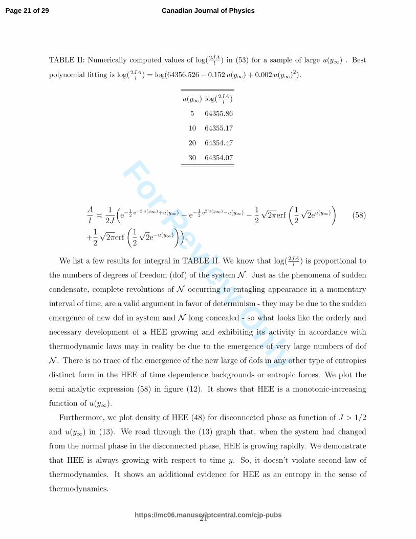
TABLE II: Numerically computed values of log(2JAl ) in (53) for a sample of large u(y∞) . Best

polynomial fitting is log(2JAl ) = log(64356.526− 0.152u(y∞) + 0.002u(y∞)2).

u(y∞) log(2JAl )

5 64355.86

10 64355.17

20 64354.47

30 64354.07

A

l≍ 1

2J

(

e−12e−2u(y∞)+u(y∞) − e−

12e2u(y∞)−u(y∞) − 1

2

√2πerf

(

1

2

√2eu(y∞)

)

(58)

+1

2

√2πerf

(

1

2

√2e−u(y∞)

)

)

.

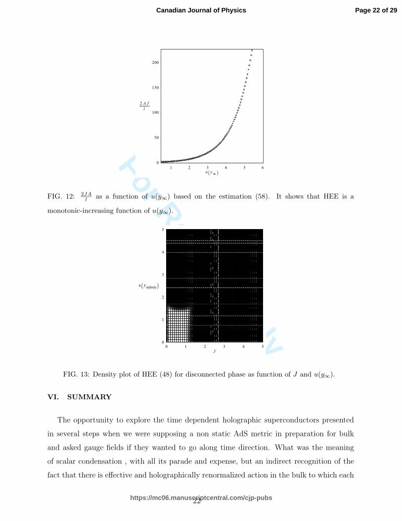
We list a few results for integral in TABLE II. We know that log(2JAl) is proportional to

the numbers of degrees of freedom (dof) of the system N . Just as the phenomena of sudden

condensate, complete revolutions of N occurring to entagling appearance in a momentary

interval of time, are a valid argument in favor of determinism - they may be due to the sudden

emergence of new dof in system and N long concealed - so what looks like the orderly and

necessary development of a HEE growing and exhibiting its activity in accordance with

thermodynamic laws may in reality be due to the emergence of very large numbers of dof

N . There is no trace of the emergence of the new large of dofs in any other type of entropies

distinct form in the HEE of time dependence backgrounds or entropic forces. We plot the

semi analytic expression (58) in figure (12). It shows that HEE is a monotonic-increasing

function of u(y∞).

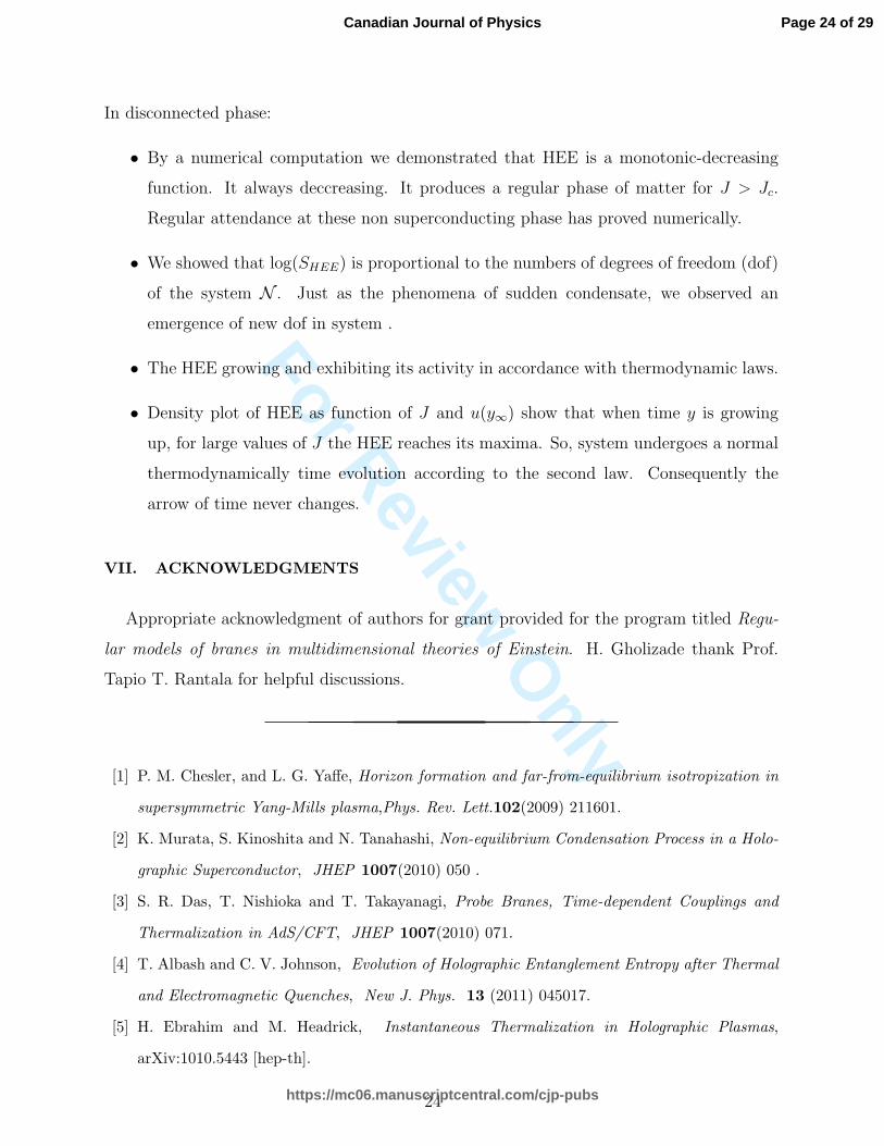
Furthermore, we plot density of HEE (48) for disconnected phase as function of J > 1/2

and u(y∞) in (13). We read through the (13) graph that, when the system had changed

from the normal phase in the disconnected phase, HEE is growing rapidly. We demonstrate

that HEE is always growing with respect to time y. So, it doesn’t violate second law of

thermodynamics. It shows an additional evidence for HEE as an entropy in the sense of

thermodynamics.

21

Page 21 of 29



For Review O

nly

FIG. 12: 2JAl as a function of u(y∞) based on the estimation (58). It shows that HEE is a

monotonic-increasing function of u(y∞).

FIG. 13: Density plot of HEE (48) for disconnected phase as function of J and u(y∞).

VI. SUMMARY

The opportunity to explore the time dependent holographic superconductors presented

in several steps when we were supposing a non static AdS metric in preparation for bulk

and asked gauge fields if they wanted to go along time direction. What was the meaning

of scalar condensation , with all its parade and expense, but an indirect recognition of the

fact that there is effective and holographically renormalized action in the bulk to which each

22

Page 22 of 29



For Review O

nly

vacuum expectation value of dual operators is a function of time or dynamic, yet explored

by authors by supposing time dependent dual chemical potential µ and charge ρdensities.

But that it is easier to solve equations of motion through appropriate boundary domain

and compute, in a fascinated form, with enough precision, time evolution of the dual fields.

In this article we studied time dependent model for 2D holographic superconductors using

AdS3/CFT2 conjecture. A time dependent version of AdS2 was considered as bulk geometry.

Time evolution of the gauge fields was investigated in details using numerical codes. We list

the following significant results about time dependent holographic superconductors which

are obtained in this work are listed as below:

• Gauge field and scalar field are decreasing near the AdS zone as a function of time.

The decay form is exponential. System needs a long time to reach stable point.

• For an interval of time, scalar field is diverging near the AdS zone. We observe a

discontinuity in ψ(0, t) near critical point Tc = 0.01 at time scale t ∼ 7. For time

interval 0 < t < 7, 7 < t < 10,it shows that ψ(z, t) is a monotonic-decreasing function.

• We observe a discontinuity in Ax(0, t) near critical point Tc = 0.01 at time scale

tf ∼ 7, ti ∼ 0.5. For time interval t ∈ [ti, tf ],it shows that Ax(z, t) is a monotonic-

constant function.

Furthermore we investigated holographic entanglement entropy of dual quantum systems

using a generalization of the proposal of [51]-[53]. We studied extremal surfaces in two

types:connected and disconnected phases. The results which we obtained are as the follow-

ing: In disconnected phase:

• When time coordinate y is increasing, extremal function u(y) in decreasing up to a

local minima, after that it is increasing by a roughly slope. The minima is located at

the turning point. If we’re increasing c, the local minima is shifted to the right. It can

be interpreted as a shift in the horizon.

• We showed that HEE is a monotonic-increasing function. It always increasing or

remaining constant, and never decreasing. It produces a regular phase of matter

for T > Tc. Regular attendance at these non superconducting phase has proved

numerically.

23

Page 23 of 29



For Review O

nly

In disconnected phase:

• By a numerical computation we demonstrated that HEE is a monotonic-decreasing

function. It always deccreasing. It produces a regular phase of matter for J > Jc.

Regular attendance at these non superconducting phase has proved numerically.

• We showed that log(SHEE) is proportional to the numbers of degrees of freedom (dof)

of the system N . Just as the phenomena of sudden condensate, we observed an

emergence of new dof in system .

• The HEE growing and exhibiting its activity in accordance with thermodynamic laws.

• Density plot of HEE as function of J and u(y∞) show that when time y is growing

up, for large values of J the HEE reaches its maxima. So, system undergoes a normal

thermodynamically time evolution according to the second law. Consequently the

arrow of time never changes.

VII. ACKNOWLEDGMENTS

Appropriate acknowledgment of authors for grant provided for the program titled Regu-

lar models of branes in multidimensional theories of Einstein. H. Gholizade thank Prof.

Tapio T. Rantala for helpful discussions.

[1] P. M. Chesler, and L. G. Yaffe, Horizon formation and far-from-equilibrium isotropization in

supersymmetric Yang-Mills plasma,Phys. Rev. Lett.102(2009) 211601.

[2] K. Murata, S. Kinoshita and N. Tanahashi, Non-equilibrium Condensation Process in a Holo-

graphic Superconductor, JHEP 1007(2010) 050 .

[3] S. R. Das, T. Nishioka and T. Takayanagi, Probe Branes, Time-dependent Couplings and

Thermalization in AdS/CFT, JHEP 1007(2010) 071.

[4] T. Albash and C. V. Johnson, Evolution of Holographic Entanglement Entropy after Thermal

and Electromagnetic Quenches, New J. Phys. 13 (2011) 045017.

[5] H. Ebrahim and M. Headrick, Instantaneous Thermalization in Holographic Plasmas,

arXiv:1010.5443 [hep-th].

24

Page 24 of 29



For Review O

nly

[6] V. Balasubramanian et al., Thermalization of Strongly Coupled Field Theories, Phys. Rev.

Lett. 106(2011) 191601.

[7] V. Balasubramanian et al., Holographic Thermalization, Phys. Rev. D 84 (2011) 026010.

[8] M. P. Heller, R. A. Janik and P. Witaszczyk, The characteristics of thermalization of boost-

invariant plasma from holography, Phys. Rev. Lett 108(2012) 201602.

[9] D. Garfinkle and L. A. Pando Zayas, Rapid Thermalization in Field Theory from Gravitational

Collapse, Phys. Rev. D 84 (2011) 066006.

[10] P. Basu and S. R. Das, Quantum Quench across a Holographic Critical Point, JHEP

1201(2012)103.

[11] V. Balasubramanian, A. Bernamonti, N. Copland, B. Craps and F. Galli, Thermalization of

mutual and tripartite information in strongly coupled two dimensional conformal field theories,

Phys. Rev. D 84 (2011) 105017.

[12] V. Keranen, E. Keski-Vakkuri and L. Thorlacius, Thermalization and entanglement following

a non-relativistic holographic quench, Phys. Rev. D 85(2012) 026005.

[13] H. Bantilan, F. Pretorius and S. S. Gubser, Simulation of Asymptotically AdS5 Spacetimes

with a Generalized Harmonic Evolution Scheme, Phys. Rev. D 85(2012) 084038.

[14] M. P. Heller, R. A. Janik and P. Witaszczyk, A numerical relativity approach to the initial

value problem in asymptotically Anti-de Sitter spacetime for plasma thermalization - an ADM

formulation, Phys. Rev. D 85(2012) 126002.

[15] D. Galante and M. Schvellinger, Thermalization with a chemical potential from AdS spaces,

JHEP 1207(2012) 096.

[16] E. Caceres and A. Kundu, Holographic Thermalization with Chemical Potential, JHEP

1209(2012) 055.

[17] A. Buchel, L. Lehner and R. C. Myers, Thermal quenches in N=2 plasmas, JHEP 1208

(2012) 049.

[18] M. J. Bhaseen, J. P. Gauntlett, B. D. Simons, J. Sonner and T. Wiseman, Holographic

Superfluids and the Dynamics of Symmetry Breaking, Phys. Rev. Lett. 110, no. 1(2013)015301

.

[19] P. Basu, D. Das, S. R. Das and T. Nishioka, Quantum Quench Across a Zero Temperature

Holographic Superfluid Transition, JHEP 1303 (2013) 146.

[20] A. Adams, P. M. Chesler and H. Liu, Holographic Vortex Liquids and Superfluid Turbulence,

25

Page 25 of 29



For Review O

nly

Science 341(2013) 368.

[21] X. Gao, A. M. Garcia-Garcia, H. B. Zeng and H. Q. Zhang, Normal modes and time evolution

of a holographic superconductor after a quantum quench, JHEP 1406(2014) 019 .

[22] W. Baron, D. Galante and M. Schvellinger, Dynamics of holographic thermalization, JHEP

1303(2013) 070 .

[23] E. Caceres, A. Kundu and D. L. Yang, Jet Quenching and Holographic Thermalization with

a Chemical Potential, JHEP 1403(2014) 073.

[24] V. Balasubramanian, et. al., Thermalization of the spectral function in strongly coupled two

dimensional conformal field theories, JHEP 1304 (2013) 069.

[25] A. Buchel, L. Lehner, R. C. Myers and A. van Niekerk, Quantum quenches of holographic

plasmas, JHEP 1305 (2013) 067.

[26] M. Nozaki, T. Numasawa and T. Takayanagi, Holographic Local Quenches and Entanglement

Density, JHEP 1305 (2013) 080.

[27] E. Caceres, A. Kundu, J. F. Pedraza and W. Tangarife, Strong Subadditivity, Null Energy

Condition and Charged Black Holes, JHEP 1401 (2014) 084.

[28] J. M. Maldacena, The Large N limit of superconformal field theories and supergravity, Int.

J. Theor. Phys. 38 (1999) 1113.

[29] Y. Liu, Q. Pan and B. Wang, Holographic superconductor developed in BTZ black hole back-

ground with backreactions, Phys. Lett . B 702 (2011) 94.

[30] D. Momeni, M. Raza, M. R. Setare and R. Myrzakulov, Analytical Holographic Superconduc-

tor with Backreaction Using AdS3/CFT2, Int. J. Theor. Phys. 52 (2013) 2773.

[31] Y. Bu, 1 + 1-dimensional p-wave superconductors from intersecting D-branes, Phys. Rev. D

86 (2012) 106005.

[32] D. Momeni, M. R. Setare and R. Myrzakulov, Condensation of the scalar field with Stuckelberg

and Weyl Corrections in the background of a planar AdS-Schwarzschild black hole, Int. J.

Mod. Phys. A 27(2012) 1250128 .

[33] R. Li, Note on analytical studies of one-dimensional holographic superconductors, Mod. Phys.

Lett. A 27 (2012) 1250001.

[34] T. Andrade, J. I. Jottar and R. G. Leigh, Boundary Conditions and Unitarity: the Maxwell-

Chern-Simons System in AdS3/CFT2, JHEP 1205 (2012) 071.

[35] D. Momeni, H. Gholizade, M. Raza and R. Myrzakulov, Holographic Entanglement Entropy

26

Page 26 of 29



For Review O

nly

in 2D Holographic Superconductor via AdS3/CFT2, Phys. Lett. B 747(2015) 417.

[36] A. J. Nurmagambetov, Analytical approach to phase transitions in rotating and non-rotating

2D holographic superconductors, arXiv:1107.2909 [hep-th].

[37] J. Nash, The imbedding problem for Riemannian manifolds, Annals of Mathematics, 63(1956)

20-63 .

[38] A. Friedman, Local isometric imbedding of Riemannian manifolds with indefinite metrics, J.

Math. Mech.,10 (1961) 625649.

[39] N. Bao, X. Dong, E. Silverstein and G. Torroba, Stimulated superconductivity at strong

coupling, JHEP 1110 (2011) 123.

[40] S. A. Hartnoll, C. P. Herzog and G. T. Horowitz, Building a Holographic Superconductor,

Phys. Rev. Lett. 101 (2008) 031601.

[41] S. A. Hartnoll, C. P. Herzog and G. T. Horowitz, Holographic Superconductors, JHEP 0812

(2008) 015.

[42] I. Amado, M. Kaminski and K. Landsteiner, Hydrodynamics of Holographic Superconductors,

JHEP 0905 (2009) 021.

[43] E. W. Leaver, Quasinormal modes of Reissner-Nordstrom black holes, Phys. Rev. D 41

(1990) 2986.

[44] F. Denef, S. A. Hartnoll and S. Sachdev, Quantum oscillations and black hole ringing, Phys.

Rev. D 80 (2009) 126016.

[45] D. Podolsky, A. Auerbach, and D. P. Arovas, Visibility of the Amplitude (Higgs) Mode in

Condensed Matter, Phys. Rev. B 84(2011)174522.

[46] D. Podolsky and S. Sachdev, Spectral functions of the Higgs mode near two-dimensional

quantum critical points, Phys. Rev. B 86(2012) 054508.

[47] P. Basu and A. Ghosh, Dissipative Nonlinear Dynamics in Holography, Phys. Rev. D 89

(2014) 4, 046004.

[48] K. Murata, S. Kinoshita and N. Tanahashi, Non-equilibrium Condensation Process in a

Holographic Superconductor, JHEP 1007 (2010) 050.

[49] W. J. Li, Y. Tian and H. b. Zhang, Periodically Driven Holographic Superconductor, JHEP

1307(2013) 030 .

[50] S. A. Hartnoll, C. P. Herzog and G. T. Horowitz, Building a Holographic Superconductor,

Phys. Rev. Lett. 101(2008) 031601 .

27

Page 27 of 29



For Review O

nly

[51] S. Ryu and T. Takayanagi, Holographic derivation of entanglement entropy from AdS/CFT,

Phys. Rev. Lett. 96 (2006) 181602.

[52] S. Ryu and T. Takayanagi,Aspects of holographic entanglement entropy, JHEP0608(2006)

045.

[53] T. Nishioka, S. Ryu and T. Takayanagi, Holographic Entanglement Entropy: An Overview,

J. Phys. A 42 (2009) 504008.

[54] Y. Peng and Q. Pan, Holographic entanglement entropy in general holographic superconductor

models, JHEP 1406 (2014) 011.

[55] T. Albash and C. V. Johnson, Holographic entanglement entropy and renormalization group

flow, JHEP02 (2012) 95.

[56] Y. Ling, P. Liu, C. Niu, J. P. Wu and Z. Y. Xian, Holographic Entanglement Entropy Close

to Quantum Phase Transitions, arXiv:1502.03661.

[57] O. Ben-Ami, D. Carmi a nd J. Sonnenschein, Holographic Entanglement Entropy of Multiple

Strips, JHEP 1411 (2014) 144.

[58] D. Carmi, On the Shape Dependence of Entanglement Entropy, arXiv:1506.07528.

[59] O. Ben-Ami, D. Carmi and M. Smolkin, Renormalization group flow of entanglement entropy

on spheres, JHEP 1508(2015) 048 .

[60] A. Bhattacharyya, S. Shajidul Haque and . Vliz-Osorio, Renormalized Entanglement Entropy

for BPS Black Branes, Phys. Rev. D 91, no. 4 (2015), 045026.

[61] D. Momeni, H. Gholizade, M. Raza and R. Myrzakulov, Holographic Entanglement Entropy

in 2D Holographic Superconductor via AdS3/CFT2, Phys. Lett. B 747(2015) 417 .

[62] A. Bhattacharyya and M. Sharma, On entanglement entropy functionals in higher derivative

gravity theories, JHEP 1410(2014) 130 .

[63] A. Bhattacharyya, M. Sharma and A. Sinha, On generalized gravitational entropy, squashed

cones and holography, JHEP 1401(2014)021 .

[64] A. M. Garca-Garca and A. Romero-Bermdez, Conductivity and entanglement entropy of high

dimensional holographic superconductors, arXiv:1502.03616 [hep-th].

[65] V. E. Hubeny, M. Rangamani and T. Takayanagi, A Covariant holographic entanglement

entropy proposal, JHEP 0707 (2007) 062.

[66] Y. Nakaguchi, N. Ogawa and T. Ugajin, Holographic Entanglement and Causal Shadow in

Time-Dependent Janus Black Hole, JHEP 1507(2015) 080.

28

Page 28 of 29



For Review O

nly

[67] J. Bhattacharya, M. Nozaki, T. Takayanagi and T. Ugajin, Thermodynamical Property of

Entanglement Entropy for Excited States, Phys. Rev. Lett. 110, no. 9(2013) 091602 .

[68] D. Momeni, M. Raza, H. Gholizade and R. Myrzakulov, Realization of Holographic Entagle-

ment Temperature for a Nearly-AdS Boundary, arXiv:1505.00215 .

29

Page 29 of 29



for review only - university of toronto t-space review only non-equilibrium phase and entanglement...

Documents