for massachusetts institute of omputer...
TRANSCRIPT

545 TECHNOLOGY SQUARE; CAMBRIDGE, MASSACHUSETTS 02139 (617) 253-5851
MASSACHUSETTSINSTITUTE OFTECHNOLOGY
LABORATORY FORCOMPUTER SCIENCE
MIT/LCS/TR-631
An Integrated Approach toDynamic Decision Making under Uncertainty
Tze-Yun Leong
August, 1994
This document has been made available free of charge via ftp from the
MIT Laboratory for Computer Science.


An Integrated Approach toDynamic Decision Making under Uncertainty
by
Tze-Yun Leong
August, 1994
Massachusetts Institute of Technology, 1994


An Integrated Approach to Dynamic Decision Making under Uncertainty
by
Tze-Yun Leong
This report is a modified version of a thesis submitted to theDepartment of Electrical Engineering and Computer Science on August 16, 1994,in partial fulfillment of the requirements for the degree of Doctor of Philosophy
Abstract
Decision making is often complicated by the dynamic and uncertain information involved.This work unifies and generalizes the major approaches to modeling and solving a sub-class of such decision problems. The relevant problem characteristics include discreteproblem parameters, separable optimality functions, and sequential decisions made instages. The relevant approaches include semi-Markov decision processes, dynamic deci-sion modeling, and decision-theoretic planning.
An analysis of current decision frameworks establishes a unifying task definition and acommon vocabulary; the exercise also identifies the trade-off between model transparencyand solution efficiency as their most significant limitation.
Insights gained from the analysis lead to a new methodology for dynamic decision makingunder uncertainty. The central ideas involved aremultiple perspective reasoning andincremental language extension. Multiple perspective reasoning supports different infor-mation visualization formats for different aspects of dynamic decision modeling. Incre-mental language extension promotes the use of translators to enhance language ontologyand facilitate practical development.
DynaMoL is a language design that adopts the proposed paradigm; it differentiates infer-ential and representational support for the modeling task from the solution or computationtask. The dynamic decision grammar defines an extensible decision ontology and supportsproblem specification with multiple interfaces. The graphical presentation conventiongoverns parameter visualization in multiple perspectives. The mathematical representationas semi-Markov decision process facilitates formal model analysis and admits multiplesolution methods. A general translation technique is devised for the different perspectivesand representations of the decision factors and constraints.
DynaMoL is evaluated on a prototype implementation, via a comprehensive case study inmedicine. The case study is based on an actual treatment planning decision for a patientwith atrial fibrillation. The problems addressed include both long-term discrimination andshort-term optimization of different treatment strategies. The results demonstrate practicalpromise of the framework.
Thesis supervisor: Peter SzolovitsTitle: Professor of Computer Science and Engineering


5
Acknowledgments
I would like to thank:
Professor Peter Szolovits, my thesis supervisor and mentor, for his guidance,encouragement, and support throughout my graduate career. I would not havemade it through without his patience and belief in me.
Dr. Stephen G. Pauker, my thesis reader, for teaching me about medical decisionanalysis in practice, and for providing me with the opportunity to learn from theDivision of Clinical Decision Making at Tufts-New England Medical Center.
Professor Alvin Drake, my other thesis reader, for his encouragement, enthusiasm,and for teaching me about precise and effective presentation of technical ideas.
Dr. Charles E. Ellis, for helping me with the case study; he has been a great teacherand domain expert.
Dr. William J. Long, my undergraduate thesis supervisor, and Professor RameshPatil, my undergraduate academic counsellor, for introducing me into the researchfield on which I shall build my professional career, and for being very supportiveand encouraging over the years.
Professor Harold Abelson for his encouragement at some critical points of mygraduate studies, and for inspiring me to be a computer scientist and a teacher.
Dr. Jon Doyle for providing me with financial support.
Past and present members of the Clinical Decision Making Group at the MIT Lab-oratory for Computer Science, for their friendships and camaraderie, and for pro-viding me with an intellectually stimulating environment. Ira Haimowitz andYeona Jang have been my good friends and colleagues through my undergraduateand graduate student life. Michael Wellman introduced me to automated decisionanalysis and has continued to be very supportive, encouraging, and enthusiastic inmy work. My current office mate, Christine Tsien, has always made our office apleasant place; she has been most understanding when I monopolized the officeduring the final phase of my thesis.
Members of the Division of Clinical Decision Making at Tufts-New England Med-ical Center, especially Dr. John Wong and Dr. Mark Eckman, for teaching meabout medical decision analysis, and Dr. Brian Kan, for his friendship and manyinteresting discussions.
All my friends who have helped and brightened my life over the years at MIT,especially Boon Seong Ang, Boon Hwee Chew, Hui Meng Chow, Heidi Danziger,

6
Choon Phong Goh, Meng Yong Goh, Shail Gupta, Beng Hong Lim, Janice McMa-hon, Kah Kay Sung, and Wai Khum Wong.
My parents, for their unbounded love and everlasting belief in me, and for theirpatience during my long absence from home.
My husband, Yang Meng Tan, for sharing the joy and suffering through graduateschool with me, for being a friend and a colleague, and most important of all, forhis love.
This research was supported by the National Institutes of Health Grant No. 5 R01LM04493 from the National Library of Medicine, and by the USAF Rome Labora-tory and DARPA under contract F30602-91-C-0018.

7
Contents
Acknowledgments 5
List of Figures 11
List of Tables 13
1 Introduction 151.1 Background and Motivations. . . . . . . . . . . . . . . . . . . . . . . . . . . . . . . . . . . . . . . . . . . . . . . . 151.2 The Dynamic Decision Problem . . . . . . . . . . . . . . . . . . . . . . . . . . . . . . . . . . . . . . . . . . . . . 161.3 The Application Domain . . . . . . . . . . . . . . . . . . . . . . . . . . . . . . . . . . . . . . . . . . . . . . . . . . . 181.4 Research Objectives and Approaches . . . . . . . . . . . . . . . . . . . . . . . . . . . . . . . . . . . . . . . . . 18
1.4.1 A Uniform Task Definition . . . . . . . . . . . . . . . . . . . . . . . . . . . . . . . . . . . . . . . . . . 191.4.2 A Common Vocabulary . . . . . . . . . . . . . . . . . . . . . . . . . . . . . . . . . . . . . . . . . . . . . 191.4.3 A General Methodology . . . . . . . . . . . . . . . . . . . . . . . . . . . . . . . . . . . . . . . . . . . . 191.4.4 A Prototype Implementation . . . . . . . . . . . . . . . . . . . . . . . . . . . . . . . . . . . . . . . . . 201.4.5 A Case Study . . . . . . . . . . . . . . . . . . . . . . . . . . . . . . . . . . . . . . . . . . . . . . . . . . . . . 20
1.5 Contributions . . . . . . . . . . . . . . . . . . . . . . . . . . . . . . . . . . . . . . . . . . . . . . . . . . . . . . . . . . . . 201.6 Report Overview . . . . . . . . . . . . . . . . . . . . . . . . . . . . . . . . . . . . . . . . . . . . . . . . . . . . . . . . . 21
2 A Survey of Current Approaches 232.1 Historical Background. . . . . . . . . . . . . . . . . . . . . . . . . . . . . . . . . . . . . . . . . . . . . . . . . . . . . 23
2.1.1 Markov and Semi-Markov Decision Processes . . . . . . . . . . . . . . . . . . . . . . . . . . . 232.1.2 Dynamic Decision Modeling . . . . . . . . . . . . . . . . . . . . . . . . . . . . . . . . . . . . . . . . . 242.1.3 Planning in Artificial Intelligence . . . . . . . . . . . . . . . . . . . . . . . . . . . . . . . . . . . . . 242.1.4 Recent Development . . . . . . . . . . . . . . . . . . . . . . . . . . . . . . . . . . . . . . . . . . . . . . . 25
2.2 An Example . . . . . . . . . . . . . . . . . . . . . . . . . . . . . . . . . . . . . . . . . . . . . . . . . . . . . . . . . . . . . 252.3 Semi-Markov Decision Processes . . . . . . . . . . . . . . . . . . . . . . . . . . . . . . . . . . . . . . . . . . . . 262.4 Dynamic Decision Modeling. . . . . . . . . . . . . . . . . . . . . . . . . . . . . . . . . . . . . . . . . . . . . . . . 34
2.4.1 Dynamic Influence Diagrams . . . . . . . . . . . . . . . . . . . . . . . . . . . . . . . . . . . . . . . . 342.4.2 Markov Cycle Trees. . . . . . . . . . . . . . . . . . . . . . . . . . . . . . . . . . . . . . . . . . . . . . . . 372.4.3 Stochastic Trees . . . . . . . . . . . . . . . . . . . . . . . . . . . . . . . . . . . . . . . . . . . . . . . . . . . 41
2.5 Planning in Artificial Intelligence . . . . . . . . . . . . . . . . . . . . . . . . . . . . . . . . . . . . . . . . . . . . 422.6 Summary . . . . . . . . . . . . . . . . . . . . . . . . . . . . . . . . . . . . . . . . . . . . . . . . . . . . . . . . . . . . . . . 44
3 A Unifying View 453.1 A Uniform Task Definition . . . . . . . . . . . . . . . . . . . . . . . . . . . . . . . . . . . . . . . . . . . . . . . . . 45
3.1.1 Problem Formulation . . . . . . . . . . . . . . . . . . . . . . . . . . . . . . . . . . . . . . . . . . . . . . . 453.1.2 Problem Solution . . . . . . . . . . . . . . . . . . . . . . . . . . . . . . . . . . . . . . . . . . . . . . . . . . 473.1.3 Problem Analysis . . . . . . . . . . . . . . . . . . . . . . . . . . . . . . . . . . . . . . . . . . . . . . . . . . 47
3.2 A Common Vocabulary . . . . . . . . . . . . . . . . . . . . . . . . . . . . . . . . . . . . . . . . . . . . . . . . . . . . 473.3 An Analysis . . . . . . . . . . . . . . . . . . . . . . . . . . . . . . . . . . . . . . . . . . . . . . . . . . . . . . . . . . . . . 48
3.3.1 Decision Ontology and Problem Structure . . . . . . . . . . . . . . . . . . . . . . . . . . . . . . 483.3.2 Solution Methods . . . . . . . . . . . . . . . . . . . . . . . . . . . . . . . . . . . . . . . . . . . . . . . . . . 623.3.3 Model Quality Metrics. . . . . . . . . . . . . . . . . . . . . . . . . . . . . . . . . . . . . . . . . . . . . . 63
3.4 Summary . . . . . . . . . . . . . . . . . . . . . . . . . . . . . . . . . . . . . . . . . . . . . . . . . . . . . . . . . . . . . . . 66

8 Contents
4 An Integrated Language Design 694.1 Desiderata of An Integrated Language . . . . . . . . . . . . . . . . . . . . . . . . . . . . . . . . . . . . . . . . 69
4.1.1 Expressive Decision Ontology. . . . . . . . . . . . . . . . . . . . . . . . . . . . . . . . . . . . . . . . 694.1.2 Formal Theoretic Basis . . . . . . . . . . . . . . . . . . . . . . . . . . . . . . . . . . . . . . . . . . . . . 704.1.3 Multiple Levels of Abstraction . . . . . . . . . . . . . . . . . . . . . . . . . . . . . . . . . . . . . . . 704.1.4 Multiple Perspectives of Visualization . . . . . . . . . . . . . . . . . . . . . . . . . . . . . . . . . 704.1.5 Extensibility . . . . . . . . . . . . . . . . . . . . . . . . . . . . . . . . . . . . . . . . . . . . . . . . . . . . . . 704.1.6 Adaptability . . . . . . . . . . . . . . . . . . . . . . . . . . . . . . . . . . . . . . . . . . . . . . . . . . . . . . 714.1.7 Practicality . . . . . . . . . . . . . . . . . . . . . . . . . . . . . . . . . . . . . . . . . . . . . . . . . . . . . . . 71
4.2 Overview of Language Design . . . . . . . . . . . . . . . . . . . . . . . . . . . . . . . . . . . . . . . . . . . . . . 714.3 DynaMoL: The Language . . . . . . . . . . . . . . . . . . . . . . . . . . . . . . . . . . . . . . . . . . . . . . . . . . 72
4.3.1 Basic Decision Ontology . . . . . . . . . . . . . . . . . . . . . . . . . . . . . . . . . . . . . . . . . . . . 734.3.2 Dynamic Decision Grammar . . . . . . . . . . . . . . . . . . . . . . . . . . . . . . . . . . . . . . . . . 764.3.3 Graphical Presentation Convention . . . . . . . . . . . . . . . . . . . . . . . . . . . . . . . . . . . . 774.3.4 Mathematical Representation. . . . . . . . . . . . . . . . . . . . . . . . . . . . . . . . . . . . . . . . . 784.3.5 Translation Convention . . . . . . . . . . . . . . . . . . . . . . . . . . . . . . . . . . . . . . . . . . . . . 79
4.4 DYNAMO: A Prototype Implementation . . . . . . . . . . . . . . . . . . . . . . . . . . . . . . . . . . . . . . 80
5 A Case Study 835.1 Management of Paroxysmal Atrial Fibrillation. . . . . . . . . . . . . . . . . . . . . . . . . . . . . . . . . . 835.2 Case Description and Clinical Questions . . . . . . . . . . . . . . . . . . . . . . . . . . . . . . . . . . . . . . 845.3 Assumptions . . . . . . . . . . . . . . . . . . . . . . . . . . . . . . . . . . . . . . . . . . . . . . . . . . . . . . . . . . . . 845.4 Assessment Objectives . . . . . . . . . . . . . . . . . . . . . . . . . . . . . . . . . . . . . . . . . . . . . . . . . . . . 85
6 Dynamic Decision Model Formulation 876.1 Dynamic Decision Modeling in DynaMoL. . . . . . . . . . . . . . . . . . . . . . . . . . . . . . . . . . . . . 876.2 Model Construction . . . . . . . . . . . . . . . . . . . . . . . . . . . . . . . . . . . . . . . . . . . . . . . . . . . . . . . 88
6.2.1 Basic Problem Characterization. . . . . . . . . . . . . . . . . . . . . . . . . . . . . . . . . . . . . . . 896.2.2 Action Space Definition. . . . . . . . . . . . . . . . . . . . . . . . . . . . . . . . . . . . . . . . . . . . . 916.2.3 State Space Definition . . . . . . . . . . . . . . . . . . . . . . . . . . . . . . . . . . . . . . . . . . . . . . 926.2.4 State Transition Specification . . . . . . . . . . . . . . . . . . . . . . . . . . . . . . . . . . . . . . . . 936.2.5 Event Variable Space Definition . . . . . . . . . . . . . . . . . . . . . . . . . . . . . . . . . . . . . . 946.2.6 Probabilistic Influence Specification . . . . . . . . . . . . . . . . . . . . . . . . . . . . . . . . . . . 956.2.7 Value Function Definition . . . . . . . . . . . . . . . . . . . . . . . . . . . . . . . . . . . . . . . . . . . 976.2.8 Constraint Management . . . . . . . . . . . . . . . . . . . . . . . . . . . . . . . . . . . . . . . . . . . . . 986.2.9 Parametric Assessment . . . . . . . . . . . . . . . . . . . . . . . . . . . . . . . . . . . . . . . . . . . . 102
6.3 Model Translation . . . . . . . . . . . . . . . . . . . . . . . . . . . . . . . . . . . . . . . . . . . . . . . . . . . . . . . 1066.3.1 Translating Event Variables and Influences . . . . . . . . . . . . . . . . . . . . . . . . . . . . . 1066.3.2 Translating Declaratory Constraints . . . . . . . . . . . . . . . . . . . . . . . . . . . . . . . . . . .1106.3.3 Translating Strategic Constraints . . . . . . . . . . . . . . . . . . . . . . . . . . . . . . . . . . . . . .112
7 Dynamic Decision Model Solution and Analysis 1137.1 Solution Methods. . . . . . . . . . . . . . . . . . . . . . . . . . . . . . . . . . . . . . . . . . . . . . . . . . . . . . . . .113
7.1.1 Value Iteration . . . . . . . . . . . . . . . . . . . . . . . . . . . . . . . . . . . . . . . . . . . . . . . . . . . .1137.1.2 Fundamental Matrix Solution . . . . . . . . . . . . . . . . . . . . . . . . . . . . . . . . . . . . . . . .1167.1.3 Other Methods . . . . . . . . . . . . . . . . . . . . . . . . . . . . . . . . . . . . . . . . . . . . . . . . . . . .116
7.2 Sensitivity Analyses . . . . . . . . . . . . . . . . . . . . . . . . . . . . . . . . . . . . . . . . . . . . . . . . . . . . . .117
8 Language Enhancement and Practical Development 1198.1 Supporting Language Extension and Adaptation . . . . . . . . . . . . . . . . . . . . . . . . . . . . . . . .119
8.1.1 Static vs. Dynamic Spaces . . . . . . . . . . . . . . . . . . . . . . . . . . . . . . . . . . . . . . . . . . 1208.1.2 Automatic State Augmentation . . . . . . . . . . . . . . . . . . . . . . . . . . . . . . . . . . . . . . 120

Contents 9
8.1.3 Limited Memory . . . . . . . . . . . . . . . . . . . . . . . . . . . . . . . . . . . . . . . . . . . . . . . . . 1218.1.4 Numeric and Ordering Constraints . . . . . . . . . . . . . . . . . . . . . . . . . . . . . . . . . . . 1218.1.5 Canonical Models of Combination . . . . . . . . . . . . . . . . . . . . . . . . . . . . . . . . . . . 1228.1.6 Presentation Convention . . . . . . . . . . . . . . . . . . . . . . . . . . . . . . . . . . . . . . . . . . . 122
8.2 Supporting Practical Development . . . . . . . . . . . . . . . . . . . . . . . . . . . . . . . . . . . . . . . . . . 1238.2.1 Editing and Specification Support . . . . . . . . . . . . . . . . . . . . . . . . . . . . . . . . . . . . 1248.2.2 Statistical Analysis. . . . . . . . . . . . . . . . . . . . . . . . . . . . . . . . . . . . . . . . . . . . . . . . 1248.2.3 Data Visualization . . . . . . . . . . . . . . . . . . . . . . . . . . . . . . . . . . . . . . . . . . . . . . . . 124
9 Conclusion 1259.1 Summary . . . . . . . . . . . . . . . . . . . . . . . . . . . . . . . . . . . . . . . . . . . . . . . . . . . . . . . . . . . . . . 125
9.1.1 The Analysis . . . . . . . . . . . . . . . . . . . . . . . . . . . . . . . . . . . . . . . . . . . . . . . . . . . . 1259.1.2 The Unifying View . . . . . . . . . . . . . . . . . . . . . . . . . . . . . . . . . . . . . . . . . . . . . . . 1269.1.3 The General Methodology . . . . . . . . . . . . . . . . . . . . . . . . . . . . . . . . . . . . . . . . . . 1269.1.4 The Prototype System . . . . . . . . . . . . . . . . . . . . . . . . . . . . . . . . . . . . . . . . . . . . . 1279.1.5 The Case Study . . . . . . . . . . . . . . . . . . . . . . . . . . . . . . . . . . . . . . . . . . . . . . . . . . 128
9.2 Related Work . . . . . . . . . . . . . . . . . . . . . . . . . . . . . . . . . . . . . . . . . . . . . . . . . . . . . . . . . . . 1299.3 Future Work . . . . . . . . . . . . . . . . . . . . . . . . . . . . . . . . . . . . . . . . . . . . . . . . . . . . . . . . . . . . 130
9.3.1 Language and System Development . . . . . . . . . . . . . . . . . . . . . . . . . . . . . . . . . . 1309.3.2 Large Scale Evaluation . . . . . . . . . . . . . . . . . . . . . . . . . . . . . . . . . . . . . . . . . . . . 1309.3.3 Automatic Construction of Transition Functions. . . . . . . . . . . . . . . . . . . . . . . . . 1309.3.4 Supporting Knowledge Based Model Construction . . . . . . . . . . . . . . . . . . . . . . 131
A Dynamic Decision Grammar 133
B Semi-Markov Decision Process: Definitions and Techniques 137B.1 Components of a Semi-Markov Decision Process . . . . . . . . . . . . . . . . . . . . . . . . . . . . . . 137
B.1.1 Time Index Set . . . . . . . . . . . . . . . . . . . . . . . . . . . . . . . . . . . . . . . . . . . . . . . . . . . 137B.1.2 State Space . . . . . . . . . . . . . . . . . . . . . . . . . . . . . . . . . . . . . . . . . . . . . . . . . . . . . . 137B.1.3 Action Space . . . . . . . . . . . . . . . . . . . . . . . . . . . . . . . . . . . . . . . . . . . . . . . . . . . . 138B.1.4 One-Step Transition Functions . . . . . . . . . . . . . . . . . . . . . . . . . . . . . . . . . . . . . . 138B.1.5 Alternate Definitions Of One-Step Transition Functions. . . . . . . . . . . . . . . . . . . 139B.1.6 Value Functions . . . . . . . . . . . . . . . . . . . . . . . . . . . . . . . . . . . . . . . . . . . . . . . . . . 144
B.2 Solutions of a Semi-Markov Decision Process . . . . . . . . . . . . . . . . . . . . . . . . . . . . . . . . . 145
C Dynamic Decision Model for the Case Study 147C.1 The Action Space. . . . . . . . . . . . . . . . . . . . . . . . . . . . . . . . . . . . . . . . . . . . . . . . . . . . . . . . 147C.2 The State Space . . . . . . . . . . . . . . . . . . . . . . . . . . . . . . . . . . . . . . . . . . . . . . . . . . . . . . . . . 147C.3 Numerical Variables . . . . . . . . . . . . . . . . . . . . . . . . . . . . . . . . . . . . . . . . . . . . . . . . . . . . . 148C.4 The Event Variable Space and Conditional Distributions . . . . . . . . . . . . . . . . . . . . . . . . . 151C.5 The Transition Values . . . . . . . . . . . . . . . . . . . . . . . . . . . . . . . . . . . . . . . . . . . . . . . . . . . . 164C.6 Solution and Analysis . . . . . . . . . . . . . . . . . . . . . . . . . . . . . . . . . . . . . . . . . . . . . . . . . . . . 165
D Glossary 169
References 171

10 Contents

11
List of Figures
Figure 1.1 A dynamic decision problem. . . . . . . . . . . . . . . . . . . . . . . . . . . . . . . . . . . . . . . . . . . 17
Figure 2.1 State transition diagrams . . . . . . . . . . . . . . . . . . . . . . . . . . . . . . . . . . . . . . . . . . . . . 26
Figure 2.2 Process trajectory diagrams . . . . . . . . . . . . . . . . . . . . . . . . . . . . . . . . . . . . . . . . . . . 27
Figure 2.3 Information flow in a semi-Markov decision process. . . . . . . . . . . . . . . . . . . . . . . 27
Figure 2.4 State transition diagram of an embedded Markov chain for the example. . . . . . . . 32
Figure 2.5 Relationships between time and stage views of decision horizons . . . . . . . . . . . . . 33
Figure 2.6 An influence diagram and its embedded information. . . . . . . . . . . . . . . . . . . . . . . . 35
Figure 2.7 A dynamic influence diagram for the example problem. . . . . . . . . . . . . . . . . . . . . . 36
Figure 2.8 Use of Markov cycle trees to model dynamic effects of decision alternatives. . . . . 38
Figure 2.9 A Markov cycle tree. . . . . . . . . . . . . . . . . . . . . . . . . . . . . . . . . . . . . . . . . . . . . . . . . 39
Figure 2.10 A stochastic tree. . . . . . . . . . . . . . . . . . . . . . . . . . . . . . . . . . . . . . . . . . . . . . . . . . . . 41
Figure 2.11 Basic manipulations in a stochastic tree. . . . . . . . . . . . . . . . . . . . . . . . . . . . . . . . . . 42
Figure 2.12 A partial search space for an AI planner. . . . . . . . . . . . . . . . . . . . . . . . . . . . . . . . . . 44
Figure 3.1 Interpretation by mapping. . . . . . . . . . . . . . . . . . . . . . . . . . . . . . . . . . . . . . . . . . . . . 48
Figure 3.2 Information flow in a partially observable semi-Markov decision process. . . . . . . 50
Figure 3.3 State transition diagram for example problem. . . . . . . . . . . . . . . . . . . . . . . . . . . . . 52
Figure 3.4 Dynamic influence diagrams representations of semi-Markov decision processes . 54
Figure 3.5 Action- and state-separable dynamic influence diagram. . . . . . . . . . . . . . . . . . . . . 56
Figure 3.6 A dynamic influence diagram with decomposable state descriptions. . . . . . . . . . . . 56
Figure 3.7 A dynamic influence diagram with chance events constituting the state transitions anddecomposed value functions. . . . . . . . . . . . . . . . . . . . . . . . . . . . . . . . . . . . . . . . . . . . . . . . . . . . . . 57
Figure 3.8 Comparing a) a Markov cycle tree and b) a state transition diagram. . . . . . . . . . . . 58
Figure 3.9 Using tunnel states to model duration dependent transitions. . . . . . . . . . . . . . . . . . 59
Figure 3.10 A Markov cycle tree involving cross-over strategy with different consequences. . . 60
Figure 4.1 Transition view for an action. . . . . . . . . . . . . . . . . . . . . . . . . . . . . . . . . . . . . . . . . . 78
Figure 4.2 Influence view for an action. . . . . . . . . . . . . . . . . . . . . . . . . . . . . . . . . . . . . . . . . . . 78
Figure 4.3 Inter-level translation by mapping. . . . . . . . . . . . . . . . . . . . . . . . . . . . . . . . . . . . . . 79
Figure 4.4 Inter-perspective translation by mapping. . . . . . . . . . . . . . . . . . . . . . . . . . . . . . . . . 80
Figure 4.5 The system architecture of DYNAMO: a prototype implementation of DynaMoL. 80
Figure 4.6 The DYNAMO interface. . . . . . . . . . . . . . . . . . . . . . . . . . . . . . . . . . . . . . . . . . . . . . 81
Figure 6.1 Basic problem characteristics of the case study (partial).. . . . . . . . . . . . . . . . . . . . . 91
Figure 6.2 An abbreviated transition view for action Quinidine in case study. . . . . . . . . . . . . . 94
Figure 6.3 Influence view for action Quinidine in case study. . . . . . . . . . . . . . . . . . . . . . . . . . . 96

12
Figure 6.4 A partial influence view in case study. . . . . . . . . . . . . . . . . . . . . . . . . . . . . . . . . . . . 99
Figure 6.5 Constant and varying risks of bleeding for warfarin in case study. . . . . . . . . . . . . 105
Figure 6.6 Final influence view after reduction by the influence translator. . . . . . . . . . . . . . . 107
Figure 6.7 Indexing convention for updating conditional distribution table.. . . . . . . . . . . . . . 108
Figure 6.8 An example to show conditional distribution table updating. . . . . . . . . . . . . . . . . 109
Figure 8.1 Asymmetric relations represented in an influence view. . . . . . . . . . . . . . . . . . . . . 123
Figure 8.2 Asymmetric relations represented in a tree view. . . . . . . . . . . . . . . . . . . . . . . . . . . 123

13
List of Tables
Table 6.1 State attribute variables and their outcomes for the case study . . . . . . . . . . . . . . . . 93Table C.1 The states and corresponding value functions. . . . . . . . . . . . . . . . . . . . . . . . . . . . 148Table C.2 Solution to long-term discriminatory problem in case study. . . . . . . . . . . . . . . . . 166Table C.3 Partial solution to short-term optimization problem. . . . . . . . . . . . . . . . . . . . . . . . 167

14

15
1 Introduction
Decision making in our daily lives is often complicated by the complex informa-tion involved. Much of this complexity arises from the context-sensitive varia-tions, the multiple levels of details, the uncertainty, and the dynamic nature of theunderlying phenomena. Therefore, to automate decision making, we need a gen-eral and effective way to represent and manage such myriad of information.
This work is about analyzing and synthesizing techniques for supportingdynamic decision making under uncertainty. On analysis, we present a uniformway to reason about a class of dynamic decision problems; we also identify a com-mon vocabulary for comparing and contrasting the major approaches to addressingsuch problems. On synthesis, we introduce a general methodology that integratessome salient features of existing techniques; the central ideas of this methodologyare multiple perspective reasoning and incremental language extension. Finally,we examine how the proposed methodology can be put into practical use.
1.1 Background and Motivations
Dynamic decision making under uncertainty concerns decision problems in whichtime and uncertainty are explicitly considered. For example, a common medicaldecision is to choose an optimal course of treatment for a patient whose physicalconditions may vary over time. Similarly, a common financial investment decisionis to determine an optimal portfolio with respect to fluctuating market factors overtime. These problems are particularly complicated if both the nature and the timeof future events are uncertain.
Research in control theory, operations research, decision analysis, artificialintelligence(AI) , and other disciplines has led to various techniques for formulat-ing, solving, and analyzing dynamic decision problems. These techniques adopt

16 1 Introduction
different assumptions, support different ontologies, and have different strengthsand weaknesses. Consequently, insights gained and advancements achieved in oneapproach often do not benefit the others. Without a unifying perspective, confusingarguments about applying different techniques and wasted efforts in re-inventingexisting technologies often result.
Recently, efforts to integrate techniques from different disciplines haveemerged [Dean and Wellman, 1991] [DT-Planning, 1994]. Most of these worksfocus on adapting a particular framework to accommodate other techniques. Nev-ertheless, this phenomenon suggests that some properties or characteristics in eachapproach supplement or complement the other approaches. To facilitate integra-tion, a uniform basis for examining and analyzing the different approaches isessential. Drawing analogy from knowledge representation research inAI, first-order predicate logic is such a common basis for analyzing the expressiveness andefficiency of deterministic representation languages.
Understanding the underlying conceptual models, instead of only the featuresof individual techniques, will contribute toward the effective design of a generalmethodology for dynamic decision making under uncertainty. On the other hand, agood methodology should be both theoretically sound and practically useful.Despite the variety of existing techniques, many of them have limited practicality.Some of the techniques are difficult to understand and apply, others impose toomany restrictive assumptions. Therefore, to improve on current techniques, theo-retical soundness and practical convenience should be simultaneously addressed.
1.2 The Dynamic Decision Problem
The general dynamic decision problem is to select a course ofaction that satisfiessomeobjectives in anenvironment. Definitions of the actions, objectives, and envi-ronment may vary,e.g., the actions can be described as continuous or discrete, theobjectives as reaching some “goal states” or maximizing some effects of theactions, the environment as differential equations or discrete states. The variationsdistinguish the techniques applicable for the problems.
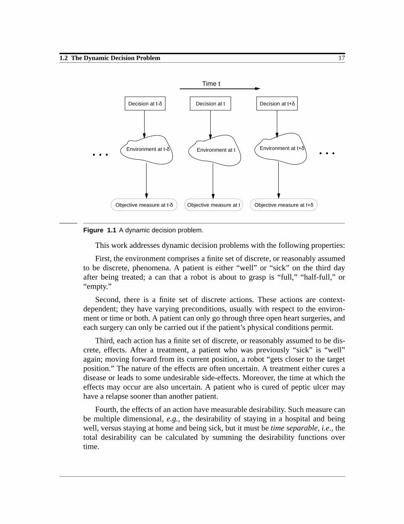
Figure 1.1 depicts the factors involved in a dynamic decision problem. Themain distinguishing feature of a dynamic decision problem from a static one is theexplicit reference of time. The environment description, the action or decisionpoints, and the objective measures are specified with respect to a time horizon.
1.2 The Dynamic Decision Problem 17
Figure 1.1 A dynamic decision problem.
This work addresses dynamic decision problems with the following properties:
First, the environment comprises a finite set of discrete, or reasonably assumedto be discrete, phenomena. A patient is either “well” or “sick” on the third dayafter being treated; a can that a robot is about to grasp is “full,” “half-full,” or“empty.”
Second, there is a finite set of discrete actions. These actions are context-dependent; they have varying preconditions, usually with respect to the environ-ment or time or both. A patient can only go through three open heart surgeries, andeach surgery can only be carried out if the patient’s physical conditions permit.
Third, each action has a finite set of discrete, or reasonably assumed to be dis-crete, effects. After a treatment, a patient who was previously “sick” is “well”again; moving forward from its current position, a robot “gets closer to the targetposition.” The nature of the effects are often uncertain. A treatment either cures adisease or leads to some undesirable side-effects. Moreover, the time at which theeffects may occur are also uncertain. A patient who is cured of peptic ulcer mayhave a relapse sooner than another patient.
Fourth, the effects of an action have measurable desirability. Such measure canbe multiple dimensional,e.g., the desirability of staying in a hospital and beingwell, versus staying at home and being sick, but it must betime separable, i.e., thetotal desirability can be calculated by summing the desirability functions overtime.
Decision at t-δ Decision at t+δDecision at t
Environment at t-δ Environment at t Environment at t+δ
Objective measure at tObjective measure at t-δ Objective measure at t+δ
Time t

18 1 Introduction
Given an initial environment, the problem is solved by choosing a course ofaction that optimizes the expected desirability of their potential effects The deci-sions are made in stages; the stages may vary in duration.
1.3 The Application Domain
While the issues we address are general, the application domain we examine isdiagnostic test and therapy planning in medical decision making. Medicine is avery rich domain for dynamic decision making under uncertainty. The multitude ofproblems, the patient-specificity, and the uncertainty involved all contribute to theintricacy of the decisions. The large, complex, and ever-changing body of medicalknowledge further complicates the process. Besides life and death decisions, max-imizing the cost-effectiveness of the actions is also important. Therefore, multipleobjective decision making is often involved; trade-offs are usually considered.
In this domain, the dynamic decision problems involve risks of some adverseevents that continue or vary over time; the events may recur and the timing of suchrecurrences are important for making the decisions. The relevant actions are diag-nostic tests and treatments, or combinations of them. The environment comprisesthe physical conditions of a patient or a class of patients. These conditions includethe physiological states of the patient, or any observable or unobservable eventsthat would lead to the states. For instance, a patient can be in a state with a stroke,and a cerebral hemorrhage may have caused the stroke. Some of these events arethe effects of the actions.
1.4 Research Objectives and Approaches
Within the scope described above, this work answers the following questions:
• What are the different tasks in dynamic decision making under uncertainty?
• What is a good basis to compare and contrast the different techniques for solv-ing the tasks?
• Can the strengths of existing techniques be integrated?
• Would such an integration improve on existing techniques?
• How can this integrated approach be practically useful?
The existing techniques relevant to this work are semi-Markov decision pro-cesses, dynamic decision modeling, andAI planning.
1.4 Research Objectives and Approaches 19
1.4.1 A Uniform Task Definition
We first define the different tasks in dynamic decision making under uncertainty asproblem formulation, problem solution, and problem analysis. The task definitionis based on analyzing the nature of the dynamic decision problems addressed, andthe current approaches to solving such problems. We present a uniform way todescribe the different aspects of a dynamic decision problem; we also illuminatethe representational and inferential support required for these aspects.
Based on this task definition, we argue that besides involving different reason-ing procedures, the different tasks also require different representational support.A vocabulary effective for supporting one task may not be effective for another.Most current techniques do not distinguish along this line.
1.4.2 A Common Vocabulary
We identify semi-Markov decision processes as a common vocabulary for analyz-ing current techniques. This common vocabulary is necessary because, in the dif-ferent frameworks, different terms or constructs may denote the same concept,while the same term may denote different concepts.
The common vocabulary provides a uniform basis to analyze the semantic andsyntactic correspondences, the strengths, and the weaknesses of the different tech-niques. Based on this analysis, we determine that the trade-off between modeltransparency and solution efficiency is the most significant limitation of currenttechniques.
1.4.3 A General Methodology
We introduce a general methodology for dynamic decision making under uncer-tainty. This new methodology motivates the design of a language design calledDynaMoL, for Dynamic decisionModeling Language. It builds on the commonbasis of current techniques, and integrates some of their salient features.
To balance the trade-off between model transparency and solution efficiency,theDynaMoL design differentiates representational and inferential support for themodeling task from the solution or computation task. The central ideas involvedare multiple perspective reasoning and incremental language extension. Multipleperspective reasoning allows us to visualize and examine the same information indifferent ways; it facilitates effective formulation and analysis of dynamic decisionproblems. Incremental language extension provides a framework that can be cus-tomized through the use oftranslators; it allows the scope of the dynamic decisionproblems addressed to be gradually expanded. The language design also admitsvarious existing solution methods and supports systematic development of suchmethods.
20 1 Introduction
1.4.4 A Prototype Implementation
We develop a prototype implementation ofDynaMoL to examine the effectivenessof the proposed methodology. The prototype system, calledDYNAMO, supportsflexible, explicit, and concise specification and visualization of decision parame-ters, and incorporates several solution methods. A user can focus on the differenttasks of dynamic decision making separately; the system will organize the relevantinformation for easy access and analysis.
1.4.5 A Case Study
We informally evaluate the effectiveness of theDynaMoL design and theDYNAMO
system with a detailed case study. The case study involves an actual clinical deci-sion situation.
Based on this case study, we demonstrate thatDynaMoL is expressive enoughto handle a class of real-life dynamic decision problems in medicine. We alsoclaim that the proposed methodology is more general than most existing tech-niques. The exercise also illuminates some desirable features and tools for a practi-cal system.
1.5 Contributions
The major contributions of this work are as follows:
First, we have established a unifying view of three major approaches todynamic decision making under uncertainty. A detailed analysis based on this viewhighlights the capabilities and limitations of each approach. These results willfacilitate choosing the correct techniques for different dynamic decision problems;they will also contribute toward effective integration and adaptation of the differ-ent techniques.
Second, we have proposed a novel language design that integrates the desirablefeatures of current techniques. By introducing a new paradigm of multiple per-spective reasoning, this design breaks the mold of single perspective reasoningsupported in all existing graphical dynamic decision modeling languages. We havealso established methods to systematically extend the language ontology. This is incontrast to the fixed vocabularies in most existing techniques.
Third, we have developed a prototype system that can handle a general class ofdynamic decision problems. We are interested in putting the system into practicaluse. Towards this end, we have documented the experiences of performing adetailed case study in a complex domain; these lessons have illuminated the toolssupport required.
1.6 Report Overview 21
Finally, this research has provided insights into the nature of, and the difficul-ties and assumptions in the class of dynamic decision problems considered. Theseresults can serve as guidelines for future research that addresses similar problemsor improves current techniques.
1.6 Report Overview
This introductory chapter has briefly summarized the research motivations andobjectives of this work. The remainder of the dissertation is organized as follows:
Chapter 2 introduces the current approaches to dynamic decision making underuncertainty, and briefly relates their developmental history.
Chapter 3 presents a uniform task definition of the dynamic decision problemsaddressed, defines a common vocabulary, and compares and contrasts the existingtechniques.
Based on the analysis, Chapter 4 discusses the desiderata and the designapproach for a general methodology that integrates the current techniques. Thecomponents ofDynaMoL and a prototype implementation are also explained.
To facilitate description of decision making inDynaMoL, Chapter 5 introducesthe domain background and decision problems for a case study. Details of the casestudy are included in Chapters 6 and 7.
Chapter 6 describes decision model formulation inDynaMoL; it examines indetail the syntax and the semantics of the language. The syntax prescribes how thedecision parameters in a dynamic decision problem can be specified and manipu-lated; the semantics includes the mathematical representation of a dynamic deci-sion problem, and a set of guidelines for interpreting the syntactic components ofthe language.
Chapter 7 examines the solution methods and the analyses supported by thelanguage.
Chapter 8 discusses the possible extensions and improvements to the languagefeatures and practical capabilities. It also sketches some approaches to such exten-sions.
Finally, Chapter 9 summarizes the achievements and limitations of this work,compares the lessons learned with related work, and proposes some ideas forfuture research.

22 1 Introduction

23
2 A Survey ofCurrentApproaches
This chapter briefly surveys three major approaches to dynamic decision makingunder uncertainty: semi-Markov decision processes, dynamic decision modeling,andAI planning. This survey mainly introduces the different techniques; it servesas a basis to a more detailed analysis on the capabilities and limitations of the tech-niques in Chapter 3.
2.1 Historical Background
Research in all the dynamic decision making methodologies addressed began inthe 1950s. Influences across disciplines were significant in the early stages, butgenerally became obscured, both to the researchers and the practitioners, as eachapproach matured and flourished. Such inter-disciplinary correspondence is againbeing noticed and exploited only recently.
2.1.1 Markov and Semi-Markov Decision Processes
Markov decision processes(MDPs) are mathematical models of sequential optimi-zation problems with stochastic formulation and state structure. Research in MDPsbegan with the ideas of [Shapley, 1953] and [Bellman, 1957], and the formaliza-tion by [Howard, 1960] and others. [Jewell, 1963] extended these results to semi-Markov decision processes(SMDPs), which are more general thanMDPs. Muchprogress has occurred since, both in extending the basic mathematical definitionsand in improving the optimization algorithms [Puterman, 1990]. The rigorous, for-mal nature of the methodology, however, renders it quite formidable to formulateand analyze complex dynamic decision problems in practice. In medicine, forinstance, while Markov and semi-Markov processes are often used for survival and

24 2 A Survey of Current Approaches
prognosis analyses,MDPs andSMDPs are seldom applied directly in clinical deci-sion making [Janssen, 1986].
2.1.2 Dynamic Decision Modeling
Drawing on a set of ideas and results closely related toMDPs, decision analysisemerged in the 1960s from operations research and game theory [Raiffa, 1968]; itis a normative problem solving framework based on probability theory and utilitytheory. By systematically formulating, solving, and analyzing a graphicaldecisionmodel, this approach helps in both gaining better insights into, as well as derivingoptimal decisions for the problem [Howard, 1988]. In recent years, some newdecision modeling formalisms have been devised to deal with dynamic decisionproblems. These dynamic decision models includedynamic influence diagrams[Tatman and Shachter, 1990],Markov cycle trees [Beck and Pauker, 1983][Hollenberg, 1984], andstochastic trees [Hazen, 1992]; they are based on struc-tural and semantical extensions of conventional decision models such as decisiontrees [Raiffa, 1968] and influence diagrams [Howard and Matheson, 1984], withthe mathematical definitions of stochastic processes.
Dynamic decision modeling is used widely in real world applications. Forinstance, it is a common tool in clinical decision making [Kassirer et al., 1987][Pauker and Kassirer, 1987] [Provan, 1992] [Provan and Clarke, 1993]. Neverthe-less, the methodology is difficult to apply. In particular, model formulation isknowledge-intensive and labor-intensive, and the graphical structures restrict theadmissible solution methods [Leong, 1993].
2.1.3 Planning in Artificial Intelligence
MDPs and dynamic decision modeling provide vocabularies for describingdynamic decision problems and computational models for choosing among deci-sion alternatives. In contrast,AI planning also addresses decision knowledge orga-nization and alternatives generation in dynamic decision problems. Motivated bythe studies of human problem solving [Newell and Simon, 1972], operationsresearch, and logical theorem proving,AI planning emerged with the works of[Newell et al., 1960] and [Fikes and Nilsson, 1971]. Early research in thisapproach focuses on representing and reasoning with complete and perfect infor-mation. Recent progress introduces imperfect information, extends the planningontology, and improves the plan-generation and plan-execution algorithms [Tateet al., 1990].
Most of the planning works, however, are theoretical. Their impracticality ispartly due to the complexity of the problems they address, and partly due to atrade-off between language expressiveness and solution efficiency. For instance, ina planning language with hierarchical representation of the actions, their effects,

2.2 An Example 25
and the relevant constraints, extra inferences are needed to derive the solutions. Onthe other hand, such representation support greatly facilitates problem formulation.
2.1.4 Recent Development
In the past few years, efforts to integrate techniques from the different approacheshave begun to emerge. This leads to a brand new research discipline ofdecision-theoretic planning. Comparative investigations of specific aspects of the differentmethodologies are gaining attention [Dean and Wellman, 1991] [Haddawy andHanks, 1990] [Haddawy and Hanks, 1992] [Wellman and Doyle, 1991] [Wellmanand Doyle, 1992]. Most of the ongoing works, however, attempt to adapt a particu-lar framework by incorporating some features of others [Dean et al., 1992] [Deanet al., 1993a] [Dean et al., 1993b] [Provan, 1992] [Provan and Clarke, 1993][Wellman et al., 1992].
2.2 An Example
To illustrate the different methodologies, we examine a dynamic decision problemin the management of chronic ischemic heart disease(CIHD)1. CIHD is a diseasethat limits blood supply to the heart muscles, and hence impairs the normal perfor-mance of the heart as the blood circulation regulator; the most common type ofCIHD is coronary artery disease (CAD). The problem, adapted and simplified from[Wong et al., 1990], is to determine the relative efficacies of different treatmentsfor chronic stable angina,i.e., chest pain, the major manifestation ofCAD. Thealternatives considered are medical therapy, percutaneous transluminal angioplasty(PTCA), and coronary artery bypass graft(CABG). The treatment efficacies are eval-uated with respect to quality-adjusted life expectancy(QALE).
CAD is usually atherosclerotic in nature. Atherosclerosis means progressiveobstruction of the arteries with the formation of plaque, which contains fattydeposits. The manifestations ofCAD, therefore, are progressive. If the angina wors-ens after a treatment, subsequent actions will be considered. Even after successfultreatment, restenosis or renewed occlusion of the arteries may occur. Hence, asequence of decisions must be made. For ease of discussion, all three treatmentsare assumed to be repeatedly applicable.
As time progresses, the treatment efficacies in lowering mortality and morbid-ity decline, and the treatment complications worsen. These might be due to theprogression of the disease, or the deteriorating status of the patient with time. Amajor complication forPTCA is perioperative myocardial infarction(MI) , which
1. A glossary of the medical concepts can be found in Appendix D.

26 2 A Survey of Current Approaches
would render an emergencyCABG necessary. Non-procedural relatedMI may alsooccur after a treatment.
In this example, therefore, the risks and benefits of the actions vary over time,some important events may recur over time, and the timing of such events areuncertain.
2.3 Semi-Markov Decision Processes
As mentioned in Section 2.1.1, anSMDP is a mathematical model of a sequentialdecision process. The decision problem is formulated in terms of a set of actions, aset of states with associated values, and a set of stochastic transition characteris-tics. The stochastic nature of the transitions are reflected in both thedestination ofthe transition and thetime lapsed before the transition. There are many subclassesof SMDPs; specializations can be along discrete or continuous time units, discreteor continuous actions, discrete or continuous states, and deterministic or stochasticinter-transition times. AnMDP is anSMDP in which the inter-transition times areconstant at one time unit.
Although the formal vocabulary ofSMDPs does not include any graphical com-ponents, a variety of graphical devices are commonly used to depict the conceptsinvolved. These include state transition diagrams, process trajectory diagrams,andinformation flow diagrams.
Figure 2.1 shows the state transition diagrams for a simple example where apatient or a class of patients can be well, sick, or dead at any point in time. Statesare depicted as circles and possible transitions as arcs connecting the circles; eachaction determines a different set of transitions.
Figure 2.1 State transition diagrams showing: a) all possible transitions; b) nexttransitions in time.
A process trajectory diagram illustrates a sample path or instance of a process,e.g., how a single patient would behave if he is governed by the process. Figure 2.2shows two process trajectory diagrams for the same simple example above. Thefirst diagram assumes variable inter-transition times; the second diagram assumesconstant inter-transition times,i.e., a Markov process. The semi-Markov processes
Well Sick
Dead
Well
Sick
Dead
Well
Sick
Dead
State at time t State at time t+1a) b)
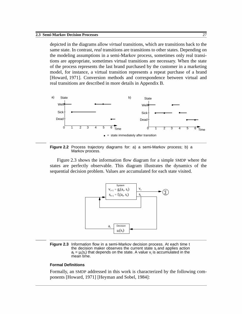
2.3 Semi-Markov Decision Processes 27
depicted in the diagrams allowvirtual transitions, which are transitions back to thesame state. In contrast,real transitions are transitions to other states. Depending onthe modeling assumptions in a semi-Markov process, sometimes only real transi-tions are appropriate, sometimes virtual transitions are necessary. When the stateof the process represents the last brand purchased by the customer in a marketingmodel, for instance, a virtual transition represents a repeat purchase of a brand[Howard, 1971]. Conversion methods and correspondence between virtual andreal transitions are described in more details in Appendix B.
Figure 2.2 Process trajectory diagrams for: a) a semi-Markov process; b) aMarkov process.
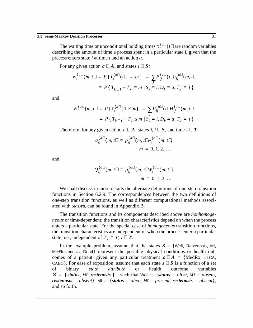
Figure 2.3 shows the information flow diagram for a simpleSMDP where thestates are perfectly observable. This diagram illustrates the dynamics of thesequential decision problem. Values are accumulated for each state visited.
Figure 2.3 Information flow in a semi-Markov decision process. At each time tthe decision maker observes the current state st and applies actionat = µt(st) that depends on the state. A value vt is accumulated in themean time.
Formal Definitions
Formally, anSMDP addressed in this work is characterized by the following com-ponents [Howard, 1971] [Heyman and Sobel, 1984]:
Time0 1 2 3 4 5 6
State
Dead
Sick
Well
Time0 1 2 3 4 5 6
State
Dead
Sick
Well
a) b)
= state immediately after transition
st+1 = ft(at, st)
System
µt(st)Decision
st
at
vt∑
vt+1 = gt(at, st)

28 2 A Survey of Current Approaches
• A time index setT;
• A decision or control process denoted by a set of random variables, where is the decision made at
time t; and
• A semi-Markov reward process denoted by a set of random variables, where is the state of the process at
time t, with:
1. an embedded Markov chain denoted by a set of random variables; such that , where are the ran-
dom variables denoting the successive epochs or instants of time at whichthe process makes transitions;
2. α sets of transition probabilitiesamong the states of the embedded chain. The transition probabilities indi-cate the fractions of (eventual) transitions from a statei to another statej,given that the process enters statei at timet, and an actiona.
For any given action , and states :
which also satisfies theMarkovian property, i.e., it does not depend on howthe process gets to the current statei:
3. α sets of holding times amongthe states of the embedded chain, which are random numbers with corre-sponding probability mass functions (PMFs):
and cumulative distribution functions (CDFs):
.
The holding times describe the amount of time the process spent in a par-ticular statei, given that the process enters statei at timet, its next transi-tion is to statej, and an actiona.
For any given action , and states :
D t( ) t T∈; D t( ) A∈ 1 2 … α, , , =
S t( ) t T∈; S t( ) S∈ 0 1 2 …, , , =
Sk k 0≥; Sk S Tk( )= T1 T2 T3 …< < <
Pija( ) t( ) i 0 j 0≥ 1 a α t T∈,≤ ≤,,≥;
a A∈ i j S∈,
Pija( ) t( ) P Sk 1+ j Sk i Dk, a Tk,= = = t = =
P S T( k 1+ ) j S T( k ) i D Tk( ),= == a Tk, t = =
Pija( ) t( ) P Sk 1+ j Sk i Dk, a Tk,= = = t = =
P Sk 1+ j Sk i Sk 1−, h … Dk, , a Tk,= = = == t =
τija( ) t( ) i 0 j 0 1 a α t T∈,≤ ≤,≥,≥;
hija( ) m t,( ) i 0 j 0 1 a α m 0 t T∈,≥,≤ ≤,≥,≥;
Hija( ) m t,( ) i 0 j 0 1 a α m 0 t T∈,≥,≤ ≤,≥,≥;
a A∈ i j S∈,

2.3 Semi-Markov Decision Processes 29
and
and
4. α sets of rewards or value functionsassociated with the states of the embedded chain, such that for any givenaction , is the value achievable in state over timedurationm.
may be defined in terms of the sets of value functions associatedwith the possible transitions ,given any action and .
Together, the transition probabilities and the holding time distributions consti-tute theone-step transition functions with PMFs:
andCDFs:
The one-step transition functions characterize the state transitions by answer-ing the following question: Given the process enters statei at timet and an actiona, how likely is it that the next transition is a transition to statej, and that the tran-sition will occur atn time units after entering state i (for thePMF), or by n timeunits after entering statei (for theCDF)?
For any given action , states , and time :
and
hija( ) m t,( ) P τij
a( ) t( ) m = =
P Tk 1+ Tk− m Sk i Sk 1+, j Dk, a Tk,= = = == t ;=
m 0 1 2 …, , ,=
Hija( ) m t,( ) P τij
a( ) t( ) m≤ =P Tk 1+ Tk− m Sk≤ i Sk 1+, j Dk, a Tk,= = == t ;=
m 0 1 2 …, , ,=
via( ) m( ) i 0 1 a α m 0≥,≤ ≤,≥;
a A∈ via( ) m( ) i S∈
via( ) m( )
vija( ) m( ) i 0 j 0 1,≥ a α m 0≥,≤ ≤,≥;
a A∈ i j, S∈
qija( ) m t,( ) i 0 j 0≥ 1 a α m 0 t,≥ T∈,≤ ≤,,≥;
Qija( ) m t,( ) i 0 j 0≥ 1 a α m 0 t,≥ T∈,≤ ≤,,≥;
a A∈ i j S∈, t T∈
qija( ) m t,( ) Pij
a( ) t( ) hija( )⋅ m t,( )=
m 0 1 2 …, , ,=P Sk 1+ j Tk 1+ Tk−, m Sk i Dk, a Tk,= = = == t ;=

30 2 A Survey of Current Approaches
In the special case of anMDP, the holding timePMFs andCDFs are:
where is the unit-impulse function; and
where is the unit-step function.
Therefore, the holding times for anMDP are all exactly one time unit in length,and the corresponding transition functions are:
;
and
.
The one-step transition functions can also be defined in terms of thecondi-tional transition probabilitiesandwaiting times with PMFs:
andCDFs:
.
The conditional transition probabilities indicate the fractions of transitionsfrom statei to another statej, given that the process enters statei at timet, makes atransition at durationm after entering statei, and an actiona.
which also satisfies theMarkovian property:
Qija( ) m t,( ) Pij
a( ) t( ) Hija( ) m t,( )⋅=
m 0 1 2 …, , ,=
P Sk 1+ j Tk 1+ Tk−,= m Sk≤ i Dk, a Tk,= == t ;=
hija( ) m t,( ) hij
a( ) m( ) δ m 1−( )= =
δ m 1−( )
Hija( ) m t,( ) Hij
a( ) m( ) 1 m 1−( )= =
1 m 1−( )
qija( ) m t,( ) qij
a( ) m( ) Pija( ) δ m 1−( )⋅==
Qija( ) m t,( ) Qij
a( ) m( ) Pija( ) 1 m 1−( )⋅==
pija( ) m t,( ) i 0 j 0≥ 1 a α m 0 t,≥ T∈,≤ ≤,,≥;
τia( ) t( ) i 0 1 a α t T∈,≤ ≤,≥;
wia( ) m t,( ) i 0 1 a α m 0 t T∈,≥,≤ ≤,≥;
Wia( ) m t,( ) i 0 1 a α m 0 t T∈,≥,≤ ≤,≥;
pija( ) m t,( ) P Sk 1+ j Sk= i Dk, a Tk, t Tk 1+ Tk−, m = = = = =
pija( ) m t,( )
P Sk 1+ j Sk i Sk 1−, h … Dk, , a Tk,= = = == t Tk 1+ Tk−, m = =
P Sk 1+ j Sk i Dk, a Tk, t Tk 1+ Tk−, m = = = = ==
2.3 Semi-Markov Decision Processes 31
The waiting time or unconditional holding times are random variablesdescribing the amount of time a process spent in a particular statei, given that theprecess enters statei at timet and an actiona.
For any given action , and states :
and
Therefore, for any given action , states , and time :
and
We shall discuss in more details the alternate definitions of one-step transitionfunctions in Section 6.2.9. The correspondences between the two definitions ofone-step transition functions, as well as different computational methods associ-ated withSMDPs, can be found in Appendix B.
The transition functions and its components described above arenonhomoge-neous or time-dependent; the transition characteristics depend on when the processenters a particular state. For the special case ofhomogeneous transition functions,the transition characteristics are independent of when the process enter a particularstate, i.e., independent of .
In the example problem, assume that the statesS = Well, Restenosis, MI,MI+Restenosis, Dead represent the possible physical conditions or health out-comes of a patient, given any particular treatment = MedRx, PTCA,CABG. For ease of exposition, assume that each state is a function of a setof binary state attribute or health outcome variables
, such thatWell := status = alive, MI = absent,restenosis = absent, MI := status = alive, MI = present,restenosis = absent ,and so forth.
τia( ) t( )
a A∈ i S∈
wia( ) m t,( ) P τi
a( ) t( ) m Pija( ) t( ) hij
a( ) m t,( )j
∑= = =
P Tk 1+ Tk− m Sk i Dk, a Tk,= = == t =
Wia( ) m t,( ) P τi
a( ) t( ) m≤ Pija( ) t( ) Hij
a( ) m t,( )j
∑= =
P Tk 1+ Tk− m Sk≤ i Dk, a Tk,= == t =
a A∈ i j S∈, t T∈
qija( ) m t,( ) pij
a( ) m t,( ) wia( ) m t,( ) ;=
m 0 1 2 …, , ,=
Qija( ) m t,( ) pij
a( ) m t,( ) Wia( ) m t,( ) ;=
m 0 1 2 …, , ,=
Tk t t T∈;=
a A∈s S∈
Θ status MI restenosis, ,=

32 2 A Survey of Current Approaches
The semi-Markov reward process, with time index set , isdefined by:
1. the embedded Markov chain as depicted in Figure 2.4;
2. three sets of transition probabilities among the states in , condi-tional on the actions in ;
3. three sets of holding timePMFs or CDFs among thestates in , conditional on the actions in ; and
4. three sets of value functions , corresponding to the amount ofQALE expected in each state in , conditional on the actions in .
Figure 2.4 State transition diagram of an embedded Markov chain for theexample. The nodes denote the states. The links represent possibletransitions from one state to another, given any treatment.
Solutions
A solution to an SMDP is an optimal policy. An optimal policy specifies the optimaldecision rule
for each that maximizes the expected value achievable in each state; a policyis stationary if it contains the same decision rule over the entire decision horizon.The optimal policies are guidelines for choosing the optimal actions over the deci-sion horizon, for all possible evolutions of the states, that maximize the expectedvalue or reward.
A variety of solution methods are available forSMDPs. The most commonalgorithms are based on thevalue iteration method of the dynamic programmingor Bellman optimality equation. A dynamic decision problem can be expressed asthe dynamic programming equation of anSMDP. Due to its complexity, we shallleave the details of this equation to Chapter 7. For now, it suffices to show the gen-eral form of the optimality equation for discrete-timeMDPs, with an arbitrary dis-count factor :
T 0 1 2 … , , ,⊆
Pija( ) .( ) S
Ahij
a( ) .( ) Hija( ) .( )
S Avi
a( ) .( )S A
Well
MI
Restenosis
MI+
Restenosis
Dead
π* µ0* µ1
* µ2* µ3
* … , , , ,= µt* : S A→
t T∈
0 β 1≤ ≤

2.3 Semi-Markov Decision Processes 33
(EQ 1)
The solution to the optimality equation is an optimal policy that maximizes, the optimal expected value or reward for an initial state,e.g.,the well
state for the example problem, at time 0.
Alternately,(EQ 1) can be reformulated as follows:
(EQ 2)
The solution to this alternate optimality equation is an optimal policy that max-imizes , the optimal expected value or reward for an initial state overduration N or N stages.
The remaining decision stages, sometimes called decision stages “to go,” indi-cates the remaining time in the decision horizon. The relationship between timeand stage is depicted in Figure 2.5.
Figure 2.5 Relationships between time and stage views of dynamic decisionproblem horizons
Note that in the Markov case, as illustrated in(EQ 1) and(EQ 2), the time vari-ablet and the duration variablen have one-to-one direct correspondence. In otherwords, the time horizon is defined as , such that
. Therefore,(EQ 2) is equivalent to:
(EQ 2’)
Other solution methods forSMDPs include policy iteration, linear program-ming,etc. Applicability of the different solution methods depends on certain prob-lem characteristics such as constant discount factor, stationary policy, andhomogeneous transition functions. Some of these methods are described in moredetails in Appendix B.
Vi* β t,( ) maxa βtvi
a( )1( ) Pij
a( ) t( ) Vj* β t, 1+( ) ;⋅
j∑+=
i j S a A t T∈,∈,∈,
Vinit* 0( )
Vi* β n,( ) maxa vi
a( ) 1( ) β Pija( ) N n−( ) Vj
* β n, 1−( )⋅j
∑+ ;=
i j S a A n,∈,∈, 0 1 2 … N, , , ,=
Vinit* N( )
TimeStage
0 1 2 tt-1...
n n-1 01...Finite
Horizon
TimeStage
0 1 ...
01...InfiniteHorizon∞
∞
T 0 1 2 3 … N, , , , , =n N t t T∈ n,;− 0 1 2 … N, , , ,= =
Vi* n β t, ,( ) maxa vi
a( ) 1( ) β Pija( ) t( ) Vj
* n 1− β t, 1+,( )⋅j
∑+ ;=
i j S a A n,∈,∈, 0 1 2 … N t T∈, , , , ,=

34 2 A Survey of Current Approaches
2.4 Dynamic Decision Modeling
A dynamic decision model is based on a graphical modeling language that depictsrelevant parameters for decision analysis in a dynamic decision problem. All thegraphical components have precise mathematical definitions. In general, such amodel consists of the following six components, the first five of which constitute aconventional decision model such as decision tree or influence diagram:
• A set ofdecision nodes listing the alternative actions that the decision makercan take, for instance, the choices of medical therapy,PTCA, andCABG;
• A set ofchance nodes, corresponding to a set of random variables, outliningthe possible outcomes or happenings that the decision maker has no controlover, for example, the physical status of the patient, the prognostic outcomes ofPTCA, and the complications ofCABG;
• A single or a set ofvalue functions, sometimes denoted asvalue nodes, captur-ing the desirability, in terms of cost, life-expectancy,etc., of each outcome oraction;
• A set ofconditional dependencies depicting how the outcomes of each chancenode probabilistically depend on other outcomes or actions;
• A set of informational or temporal dependencies indicating the informationavailable when the decision maker makes a decision; and
• An underlyingstochastic process governing the evolution in time for the abovefive components.
The stochastic processes underlying existing dynamic decision modelingframeworks are specializations ofsemi-Markov processes. The definition of asemi-Markov process is similar to that in Section 2.3, except without the decisioncomponent.
A solution to a dynamic decision model is a course of optimal action that max-imizes the value functions. The solution, derived byevaluating the model, usuallyinvolves interleaving chance nodes expectation and decision nodes maximization.
We briefly examine three types of dynamic decision models for the exampleproblem. The embedded Markov chains for the semi-Markov processes underlyingthese models are identical to the one shown in Figure 2.4.
2.4.1 Dynamic Influence Diagrams
An influence diagram is a graphical stochastic model that can explicit display con-ditional and temporal dependencies in a decision problem. An influence diagram isahierarchical representation; it has a qualitative layer and a quantitative layer. Thequalitative level is a directed graph with no cycles; it summarizes the relationsamong the decision parameters. The nodes in the graph correspond to the parame-

2.4 Dynamic Decision Modeling 35
ters in the model; the links represent the relations among the parameters. Thequantitative level includes the embedded information in the nodes. Embedded ineach chance node or value node is a list of possible outcomes or values, and a tableof probabilities conditional on its probabilistic predecessors. Embedded in eachdecision node is a list of the alternate treatments and a list of its informational pre-decessors.
Figure 2.6 shows a simple influence diagram. The notation depicts rectanglesas decision nodes, ovals as chance nodes, and diamonds as value nodes. The linksleading into the chance and value nodes indicate conditional dependence; the linksleading into the decision nodes indicate informational or temporal dependence.The absence of links between any pair of nodes indicates conditional or temporalindependence.The diagram is interpreted as follows: Random variablesx andy areindependent;z is conditioned ony. The decision maker will know the outcome ofxbefore decisiond is made; the decision will affect the outcome ofy. The objectiveis to optimize the expected value ofV, which is conditioned ond, x, andz.
Figure 2.6 An influence diagram and its embedded information.
Dynamic influence diagrams [Tatman and Shachter, 1990] extend influencediagrams by allowingtime-separable value functions; each component value func-tion measures the value achievable in a single time unit or decision stage. Adynamic influence diagram has the same kinds of graphical components as aninfluence diagram as shown in Figure 2.6, except that there will be several compo-nent or non-terminal value nodes, and a terminal value node. The relationshipbetween the non-terminal value nodes , wheren is the time index or decisionstage, and the terminal value nodeV has one of the following forms:
or
x y z
d
V
d:alternatives: (A1, A2)predecessors: (x)x:outcomes: (X, Not-X)probs: 0.1 0.9y:outcomes: (Y, Not-Y)
probs:0.2 0.8
0.7 0.3
conditioning-outcomes: (A1, A2)
z:outcomes: (Z1, Z2, Z3)
probs:0.1 0.3 0.6
0.5 0.2 0.2
conditioning-outcomes: (Y, Not-Y)
V:values: f(d, x, z)
(read:Y|A1 Not-Y|A1
Y|A2 Not-Y|A2 )
vn
V vnn∑= V vn
n∏=

36 2 A Survey of Current Approaches
Figure 2.7 shows a dynamic influence diagram for the example problem. Thenumber at the end of each node indicates the decision stage “to go,” in which theparameter is considered. Each decision stage corresponds to the time intervalbetween two successive actions, which also indicates two successive transitions inthe underlying discrete-time Markov chain; the time intervals may be in any unitand are usually constant within the model. The diagram indicates a decision hori-zon of three time units. At the beginning of the decision horizon, a decision ismade based on whetherCAD or MI or both are present, and also whether the patientis alive. At each subsequent decision stage, the decision is made based on whetherrestenosis orMI or both have occurred.
Figure 2.7 A dynamic influence diagram for the example problem.
Solutions
In a dynamic influence diagram, the decision problem is solved by graph reduc-tions through a series ofvalue preserving transformations. These reductions ortransformations preserve the joint probability distribution, the optimal course ofaction, and the expected value of the influence diagram by removing the decisionnodes, chance nodes, and non-terminal value nodes.
There are five basic transformations in solving a dynamic influence diagram[Shachter, 1986] [Tatman and Shachter, 1990]:
Barren Node Removal
A barren node is a chance node with no successors. The distribution of such anode does not affect the joint probability distribution of the diagram. Hence, a bar-
Status 3
CAD 3
Status 2 Status 1 Status 0
MI 2 MI 1 MI 0
Decision 3 Decision 2 Decision 1
Restenosis 2 Restenosis 1 Restenosis 0
Value 2
Value
Value 3 Value 0Value 1
MI 3
Decision stage n

2.4 Dynamic Decision Modeling 37
ren node can be removed from the diagram without any consequence. If theremoval of a barren node causes other nodes to become barren, they can beremoved as well.
Arc Reversal
Arc or link reversal between two chance nodes corresponds to applying Bayestheorem, when there is no other path between the two chance nodes. The twonodes involved inherit each others’ predecessors.
Chance Node Removal
Chance node removal corresponds to conditional expectation. We first add thepredecessors of the chance node to the list predecessors of its single successor.When the chance node has another chance node as its successor, we eliminate thechance node by summing its outcomes out of the joint probability distribution.When the chance node has a value node as its successor, we eliminate the chancenode by calculating its expected value.
Decision Node Removal
When a decision node has a value node as its single successor, and all otherconditional predecessors of that value node are informational predecessors of thedecision node, the decision node can be removed by maximizing the expectedvalue of its alternatives.
Non-terminal Value Node Removal
Finally, non-terminal value node removal corresponds to summing or multiply-ing the value into the terminal value node.
In addition to introducing the notion of time-separable value nodes, [Tatmanand Shachter, 1990] also provide a well established algorithm for solving dynamicinfluence diagrams. In order to take advantage of a much larger collection of eval-uation algorithms, recent efforts have tried to translate these models into Bayesianor probabilistic networks [Shachter and Peot, 1992]; all these algorithms, however,areNP-hard [Cooper, 1990] with respect to the size of the models.
2.4.2 Markov Cycle Trees
A Markov cycle tree models the dynamic effects of a decision alternative in theconventional decision tree. A Markov cycle tree does not represent a completedynamic decision problem itself. Instead, it is part of a larger model which usuallyinvolves as many cycle trees as there are decision alternatives. Figure 2.8 showsthe common use of Markov cycle trees in a dynamic decision model. Although thecycle trees in the same model may be different in principle, they usually have thesame structure in practice.

38 2 A Survey of Current Approaches
Figure 2.8 Use of Markov cycle trees to model dynamic effects of decisionalternatives.
Graphically, a Markov cycle tree is similar to a conventional decision tree. It isa single level representation; the qualitative information and the quantitative infor-mation are depicted simultaneously. The qualitative information, in terms of a setof nodes and links, summarizes the decision parameters and their relations; thequantitative information reflects the actual conditional probabilities and values.The nodes represent the decision parameters. No decision nodes are allowed in acycle tree. The chance nodes represent random variables. The state nodes, whichhave associated values, represent the states in the underlying embedded discrete-time Markov chain. The links indicate the outcomes of the chance nodes, and theconditional and temporal dependencies among these outcomes and the states. Con-ditional and temporal independence, however, are not explicitly displayed. Theconditional probabilities among the outcomes of the chance nodes, conditioned onthe specific action modeled by the cycle tree, are associated with the links.
Figure 2.9 depicts a Markov cycle tree for the example problem; three cycletrees with the same structure, but different quantitative information, are attached tothe end of the decision alternatives for the conventional decision tree with a singledecision node. The cycle tree models the possible state transitions in the embeddedMarkov chain in a decision stage, conditional on the specified action. All possiblecombinations of the chance events that could happen at each decision stage, orbetween any two transitions of the underlying Markov chain, are represented inbetween the root and the leaves of the cycle tree. The inter-transition time intervalsare constant. The cycle tree structure usually remains constant over time, only thequantitative information may change for each decision stage,e.g., with time-vary-ing transition probabilities. This prevents the size of the tree from “exploding”over time.
MedRx
PTCA
CABG
Markov cycle tree
Markov cycle tree
Markov cycle tree

2.4 Dynamic Decision Modeling 39
Figure 2.9 A Markov cycle tree.The symbol denotes the root of the cycletree, and each a leaf, i.e., the state to start in the next cycle.The label DieASR means die of all other causes, conditioned only onthe age, sex, and race of the patient.
Solutions
The solution to a dynamic decision model with Markov cycle trees determines thesingle optimal action or decision alternative over time; this is done by calculatingand comparing the values achievable over time from the respective cycle trees.Two common solution methods for Markov cycle trees arecohort analysis [Beckand Pauker, 1983] andMonte Carlo simulation; both are simulation methods, andindividual simulations are conducted for each cycle tree in the model.
In cohort analysis, the simulation begins with a hypothetical cohort in someinitial distribution, with respect to the root of the cycle tree, among the states. Forinstance, some patients who have undergonePTCA begin in theWell state, others inthe MI state due to perioperative complication. In each decision stage or “cycle,”the fraction of cohort in each state is partitioned among all the states according tothe transition probabilities specified through the intermediate chance events. Forinstance, with reference to Figure 2.9, the transition probability from theWell stateto theMI state, conditioned onPTCA, is:
MedicalTherapy
PTCA
CABG
DieASR
Survive
Restenosis
Stay Well
MI
No MI
MI
No MI
MI+Restenosis
Dead
Restenosis
MI
Well
Well
DieASR
Survive
Die Restenosis
Stay WellMI
No MI
Dead
Dead
MI+Restenosis
Restenosis
Restenosis
DieASR
Survive
Die MI
Stay WellRestenosis
No Restenosis
Dead
Dead
MI+Restenosis
MI
MI
DieASR
Survive
Die MI
Stay WellDie Restenosis
Stay Well
Dead
Dead
Dead
MI+Restenosis
MI+Restenosis
DeadDead
<state>

40 2 A Survey of Current Approaches
This results in a new distribution of the cohort among the states. As each individ-ual of the cohort passes through a state, value is accumulated for the passage. Ateach decision stage, the expected values accumulated, calledcycle sum, are:
where n is the decision stage index, ,, is the value
achievable in states, conditioned on actiona, for over a single decision stage, and is the fraction of the cohort in states at decision stagen, given actiona.
The next cycle starts with a new distribution at the root of the cycle tree. Theexpected values are accumulated until the process converges, or when theDeadstate reaches probability 1. The final result, or the expected values achievable overtime for the specified action, is:
The evaluation may take an arbitrarily long time to terminate, or it may not termi-nate at all.
In Monte Carlo simulation, the simulation involves a large number of individ-ual trials. Each individual begins in a starting state, for instance, theWell state. Atthe end of each decision stage, a random-number generator guided by the transi-tion probabilities determines the next state of the individual. Values are accumu-lated as the individual passes through each state. The trial stops when theindividual enters anabsorbing state such as theDead state. The process is repeatedmany times to derive a distribution of the values achievable; the mean of this dis-tribution is the expected value achievable for the specified action.
Both cohort analysis and Monte Carlo simulation areforward induction pro-cesses; the problem is solved by starting at the initial stage or time, and movingforward one stage at a time, until all stages are included. This contrasts with thebackward induction process, where the problem is solved by starting at the finalstage, and moving back one stage at a time, until all stages are included. Forwardinduction is applicable in a Markov cycle tree because there are no decisions orchoices involved, except at the very beginning. In other words, there is no futureoptimization involved. In general, forward induction cannot address optimizationover time problems because there is no way to compare future values in the pro-cess. It can, however, be augmented with auxilliary constructs to address some his-tory-dependent problems; this may be useful for alleviating the restrictive“memoriless” Markov assumption in such cases.
pPTCA Well MI→( ) pPTCASurvive pPTCAStaywell pPTCAMI⋅⋅=
Vna( ) frs n,
a( ) vsa( ) 1( )⋅
s∑=
a MedRx PTCA CABG,, ∈s Well MI Restenosis MI Restenosis Dead,+,,, ∈ vs
a( ) 1( )
frs n,a( )
V a( ) Vna( )
n 0=
∞
∑=

2.4 Dynamic Decision Modeling 41
2.4.3 Stochastic Trees
A stochastic tree is the continuous time version of a Markov cycle tree; it models acontinuous-time Markov chain. The inter-transition time intervals between anytwo states i and j, given an action a, are exponentially distributed:
, with specific rater and time intervalτ.
Figure 2.10 depicts a stochastic tree for the example problem. With referenceto the embedded Markov chain in Figure 2.4, only transitions to immediate statesare depicted in the stochastic tree. The bracketed state names,e.g.,[Well], indicatecyclic notations; in other words, when a bracketed state is reached, subsequentevolution starts from the point of the stochastic tree where that state is first located.Transition rates, instead of transition probabilities, are used to specify the probabi-listic characteristics of the tree. A transition rate describes the number of occur-rences of an event, per unit time, for a population of specific size; it ranges fromzero to infinity.
Figure 2.10 A stochastic tree. Parameters on the arcs indicate transition ratesamong the states.
Solutions
The solution to a dynamic decision model with stochastic trees determines the sin-gle optimal action or decision alternative over time; this is done by calculating andcomparing the values achievable over time for the respective stochastic trees. Themost common solution method is value iteration, analogous to that described in(EQ 1) and(EQ 2) for MDPs. In value iteration, the stochastic tree is rolled back. Theexpected value of each state is calculated by value expectation in the subtree withthe state in concern as the root, along the branches from the leaves. The basicmanipulations involved, as summarized in Figure 2.11, are based on the “memori-less” property of the exponential distributions [Taylor and Karlin, 1994]. Moreintuitively, a process waiting in states until it makes a transition to a specific desti-nation is equivalent to waiting in states until a transition occurs and then determin-ing the identity of the destination [Hazen, 1992].
Hija( ) τ( ) 1 e rτ−−=
MedicalTherapy
PTCA
CABG
Well
Dead
MI
Restenosis
Dead
MI + Restenosis
Dead
[Well]
MI + Restenosis
Dead
µ0
λm
µ0 + µm
λr µ0 + µm +µr
Deadµ0 + µm +µr
µ0 + µr
λr λw
λm

42 2 A Survey of Current Approaches
Figure 2.11 Basic manipulations in a stochastic tree. The fractions pi’s are definedby pi = ri / Σi ri.
The expected values achievable for a specific action can be expressed in termsof the optimality equation as follows:
where ,, is the value achievable in states per unit time,
conditioned on actiona, is the transition rate from states, and .
With reference to Figure 2.10, for instance:
If cycles appear in the state transition diagram of the embedded Markov chain,the evaluation must be done across several cycles until the numbers converge. Dueto the decomposability of the exponential transition time functions, fewer calcula-tions are required as compared to Markov cycle tree evaluation, and the evaluationterminates in finite time.
2.5 Planning in Artificial Intelligence
In classicalAI planning, the dynamic decision problem consists of an initial state, agoal state, and a set of operators. The typical operators, originating from the plan-ner STRIPS [Fikes and Nilsson, 1971], characterize actions or events (actions ofnature) in terms of their preconditions and their effects. An operatorω can bedescribed as a set of pairs < α, β >, whereα is a set of preconditions andβ is a setof effects or postconditions. The preconditions are propositions or conditions thatmust hold before the operator can be applied; the postconditions are propositionsor conditions that must hold after the operator is applied. Each propositiondescribes a subset of the states involved; the states may or may not be fully enu-merated. In other words, each proposition describes an attribute or dimension of
S
S1
S2
S3
r1
r2
r3
S
S1
S2
S3
p2
p3
r ii∑Superposition
Decomposition
p1
Via( ) 1
r jj∑vi
a( )⋅ pj Vja( )⋅
j∑+=
i j, Well MI Restenosis MI Restenosis Dead,+,,, ∈a MedRx PTCA CABG,, ∈ vs
a( )
rs ps rs rss∑⁄=
VM I+RestenosisPTCA 1
µ0
µm
µr
+ + vMI+RestenosisPTCA⋅ VDead
PTCA+=
VMIPTCA 1
µ0
µm
µr
+ + vMIPTCA⋅
λr
µ0
µm
µr
+ + VM I+RestenosisPTCA⋅
µ0
µm
+µ
0µ
mµ
r+ + VDead
PTCA⋅+ +=

2.5 Planning in Artificial Intelligence 43
the state definitions. A plan is a sequence of operators; it is the solution to thedynamic decision problem if the plan is applicable in the initial state, and the goalstate is true after executing the plan [Tate et al., 1990].
ClassicalAI planning assumes deterministic action effects and absolute utilityor value of the goal state. In other words, if the preconditions of an action operatorare satisfied, after the operator is applied, its postconditions are guaranteed to besatisfied. Moreover, reaching a goal state or satisfying a set of objectives can eithersucceed or fail; there is no notion of optimality.
Recent research in decision-theoretic planning has led to a number of planningframeworks that incorporate decision theoretic methods. Many of these techniquesaddress dynamic decision problems that can be described in terms ofMDPs. Thesetechniques, therefore, are directly relevant to this work.
In a decision-theoretic planner, an operatorω can be described as a set of tri-ples < α, ρ, β >, whereα is a set of preconditions,β is a set of postconditions, andρ is a probability indicating how likelyβ will be satisfied afterω is applied[Hanks, 1990] [Draper et al., 1994] [Kushmerick et al., 1994]. For instance:
Operator(PTCA) = <Restenosis, 0.8, Well>, < Restenosis, 0.15, Restenosis>,<Restenosis, 0.05, Dead>
Most of the research inAI planning focuses on efficiently representing andsolving dynamic decision problems with large and complex state space. On repre-sentations, decomposable representation techniques of action effects or statedescriptions are emphasized. On solutions, feasible ways of trading off optimalityfor speed, and improving such trade-offs, are addressed.
In the generalSMDPs and dynamic decision modeling approaches describedearlier, problem formulation and solution are in terms of explicitly and exhaus-tively enumerated action space and state space. InAI planning, however, problemformulation and solution involve on-demand generation of the action space andstate space.AI planners, therefore, usually need to address theramification prob-lem, thequalification problem, and theframe problem. The ramification problemdeals with the representation of complex action effects. The qualification problemconcerns the necessary preconditions for an action to achieve specific effects.Theframe problem addresses the invariant conditions after applying an action.
Solutions
Solution methods in classicalAI planning are based onheuristic search[Korf, 1987]. Guided by a set of heuristics, plan generations often involve actionand state spaces at multiple levels of abstraction. The appropriate heuristicsdepend on the planning ontology of the framework.
In decision-theoretic planning, many solution methods that aim to provide fastanswers at the cost of optimality are based on generating partial plans and system-

44 2 A Survey of Current Approaches
atically improving on such plans. This approach is similar to the policy iterationmethod inMDPs [Howard, 1960].
Figure 2.12 depicts a partial search space for the example problem. The mostcommon solution approach is to heuristically determine the size of the searchspace and the direction of search. The objective of the search is to find an optimalcourse of action. Optimality is usually defined in terms of maximizing probabili-ties or minimizing time. In the diagram, the oval nodes represent the states, thesquare nodes the actions. Links leading into the chance nodes indicate conditionaldependencies, links leading into the action nodes indicate informational dependen-cies. Transition probabilities and other parameters such as transition times areassociated with the conditional links. A decision stage spans between any twoactions separated by a state. The propositions or state attributes that are relevantare labelled besides the states; unmentioned propositions are assume to be eitherirrelevant or unchanged from possible previous decision stage.
Figure 2.12 A partial search space for an AI planner.
2.6 Summary
We have so far sketched the basic framework in three approaches to dynamic deci-sion making under uncertainty. In the next chapter, we shall examine the common-alities, the differences, and the strengths and weaknesses of the techniques in termsof their decision ontologies and problem structures, solution methods, and avail-able metrics for assessing model quality.
Status(Alive)
Restenosis(T)MI(T)
Restenosis(T)MI(F)
Restenosis(F)MI(T)
Restenosis(F)MI(F)Status(Dead)
Restenosis(T)MI(T)
Restenosis(T)MI(F) Restenosis(F)
MI(T)Restenosis(F)
MI(F)Status(Dead)
PTCA
CABG
MedRx
PTCA CABG MedRx
0.80.05
0.05 0.050.05

45
3 A Unifying View
Based on the survey in Chapter 2, we present a unifying view for reasoning aboutthe class of dynamic decision problems addressed in this work. We first define auniform task definition of dynamic decision making under uncertainty, and thenidentify a common vocabulary for the existing methodologies. This unifying viewestablishes a basis for comparing and contrasting the different techniques. Threemajor arguments result from this exercise. First, there are well-defined correspon-dence among the different methodologies. Second, by building on their commonbasis, we can integrate the desirable features of these techniques to form a soundand flexible framework. Third, we can extend this integration to support a new par-adigm of dynamic decision making under uncertainty; the central ideas involvedmultiple perspective reasoning and incremental language extension. We claim thatthis paradigm generalizes current approaches.
3.1 A Uniform Task Definition
The three major tasks in dynamic decision making under uncertainty are problemformulation, solution, and analysis. Problem formulation defines the decision envi-ronment or context by specifying the relevant parameters and their interrelation-ships. Problem solution prescribes a course of optimal action given the decisioncontext. Problem analysis supports validation and verification of the decisionparameters and solutions. The three tasks may interleave and may repeat manytimes for a given problem.
3.1.1 Problem Formulation
Formulating a dynamic decision problem begins with representing and specifyingthe decision factors and constraints involved. Examples of decision factors include

46 3 A Unifying View
alternative actions and strategies, possible state transitions, chance events that con-stitute the state transitions, and relevant probability distributions with respect totime. Examples of decision constraints include applicability conditions of theactions, validity conditions of the states, and logical statements about the statesand chance events. This modeling task is supported by the decision ontology orvocabulary. The defining characteristics of a decision ontology are its expressive-ness, its succinctness, and its transparency.
Expressiveness of a decision ontology defines how accurately we can specifythe factors and constraints in a decision situation; it determines the types and orga-nization of the relevant parameters and their interrelationships. For example, adecision ontology may include only actions and states as basic concepts and tem-poral dependences as basic relations, while another may also include events andprobabilistic dependences. Similarly, a decision ontology may represent actions asindividual concepts, while another may support reasoning with classes of actions.
Succinctness of a decision ontology determines how easily we can specify thefactors and constraints in a decision situation. For example, inSMDPs and dynamicdecision models, all the states in a dynamic decision problem have to be explicitlyenumerated; inAI planning, only the relevant conditions or attributes of the statedescriptions are specified in the operators. Some features that would contribute tosuccinctness include decomposable or hierarchical descriptions, and explicit con-straint declarations. An example of hierarchical description is the taxonomic orga-nization of decision parameters such as actions, states, and chance events. Anexample of constraint declaration is a statement analogous to a logical and quanti-fied sentence or well-formed formula in predicate calculus.
Transparency of a decision ontology reflects how efficiently we can drawinferences on the information involved in a decision situation, and how easily wecan comprehend such information. An ontology with a simple syntax or semanticsdoes not necessarily imply that it is transparent; unless it is succinct, it may requiremany terms and sentences to specify a small piece of knowledge. Some featuresthat would contribute to transparency include constant representation and multipleperspective visualization.
Constant representation means the same piece of information is interpreted inthe same way or with minimal changes at all times. In order to reduce computa-tional costs or to promote precision, for instance, the same qualitative structure in amodel may be reused with different quantitative bindings or values. While justifiedand preferred sometimes, such a practice often obscures the content of the infor-mation involved, especially when the changes involved are qualitative or implicit.
Multiple perspective visualization facilitates access to the same piece of infor-mation in different ways, depending on the situations or needs. This is analogousto viewing the world with different pairs of lenses, each providing a perspectivemost natural to a particular task.

3.2 A Common Vocabulary 47
3.1.2 Problem Solution
The solution to a well-formed dynamic decision problem is a course of action thatoptimize some objectives in the decision context. The solution format can beclosed-loop or open-loop. A closed-loop solution solves the problem with respectto a specific initial point and a specific end point. A plan generated by a classicalAI
planner for a starting state and a goal state is a closed-loop solution. An open-loopsolution solves the problem with respect to all possible initial points and all possi-ble end points. A policy determined in a semi-Markov decision process (SMDP) isan open-loop solution.
The solution task involves choosing an appropriate solution method and exe-cuting the method accordingly. A solution method is a computational model thatmanipulates the information in the decision context. Unlike the modeling task inproblem formulation, problem solution assumes a complete, explicit organizationof the decision factors and constraints. In other words, given a well-formed model,the solver does not need to know how the information organization arises in thefirst place.
3.1.3 Problem Analysis
Both the formulation and the solution of a dynamic decision problem may requireanalysis of the decision factors and constraints involved. In problem formulation,analysis ensures accuracy and conciseness of the model. In problem solution, anal-ysis supports revision and refinement of the result, via revision and refinement ofthe problem formulation; it also illuminates important characteristics of the prob-lem and the solution method.
The most common analysis technique is sensitivity analysis. Sensitivity analy-sis can be divided into deterministic sensitivity and stochastic sensitivity. Deter-ministic sensitivity is reflected through adjustments of the qualitative informationinvolved; it determines which uncertain events affect the choice and the value ofthe decision. Stochastic sensitivity is reflected through adjustments of the quantita-tive information involved; it reveals how uncertain events affect the choice andvalue of the decision.
3.2 A Common Vocabulary
In addition to a uniform task definition, we need a common basis to compare andcontrast the existing techniques. Just as first-order predicate calculus serves as thebasis for most deterministic knowledge representation research inAI, we proposethat SMDPs, as described in Section 2.3, serve the same role for the class of deci-sion making techniques relevant to this work. We substantiate this argument in thenext section with a detailed analysis of the techniques described in Chapter 2. Weshall interpret the language components of the other frameworks in terms of the

48 3 A Unifying View
mathematical constructs ofSMDPs. In other words, we shall define a set of inter-pretation or mapping functions for each technique concerned as shown inFigure 3.1.
Figure 3.1 Interpretation by mapping. Each arrow type indicates atransformation function or correspondence rule.
3.3 An Analysis
Based on the uniform task definition and the common vocabulary, we examine thecapabilities and limitations of the techniques outlined in Chapter 2. In particular,we compare and contrast the decision ontology and problem structure involved in,and the solution methods and model quality metrics available for the differenttechniques. For each technique, the first and second dimensions support problemformulation, and the third and fourth dimensions support problem solution andproblem analysis.
3.3.1 Decision Ontology and Problem Structure
In this section, we analyze the decision ontology and the problem structure of theexisting techniques. The decision ontology comprises the basic language compo-nents of each technique. The problem structure describes how these componentscan be combined together to formulate a dynamic decision problem, and theassumptions and constraints involved in the combination. These two dimensionsilluminate the expressiveness, succinctness, and transparency of a language,thereby indicating its effectiveness in supporting problem formulation.
Semi-Markov Decision Processes
Recall from Section 2.3, anSMDP has the following basic components: a timeindex setT, an action spaceA, a state spaceS, a set of one-step transition functions
Current Methodology Semi-Markov Decision Process
state
state-space-at-n
transition
state-node-1
chance-node-1
transition-1-2
state-node-2
influence-n-1
γsγs
γt
influence-1-n+1
γi

3.3 An Analysis 49
with PMFs andCDFs defined in terms of either 1) a set of transi-
tion probabilities and a set of holding times withPMFs andCDFs
, or 2) a set of conditional transition probabilities and a set of
waiting times withPMFs andCDFs , and a set of value functions
. The stochastic processes defined on these basic components, based on
the embedded Markov chain , include a decision process
and a semi-Markov reward process .
The descriptions given so far summarize the basic definitions for non-homoge-neousSMDPs. Although we will not address them in detail in this work, more gen-eral classes ofSMDPs provide direct expression of the following concepts1:
• Varying action space and state space with respect to time, e.g., action a isapplicable only at timet and states is valid only at timet:
• Varying action space with respect to state,e.g., actiona is applicable only instates.
• Varying action space with respect to both state and time,e.g., actiona is onlyapplicable in states at timet:
where
• Partially observable states, which means that the decisionsare made based on some observations , but not the states
. The states and the observations, however, are related by con-ditional probability distributions . Figure 3.2 showsthe information flow diagram of a partially observableSMDP.
1. Some of these extended definitions are included in Appendix B.
qija( ) .( ) Qij
a( ) .( )
Pija( ) .( ) hij
a( ) .( )
Hija( ) .( ) pij
a( ) .( )
wia( ) .( ) Wi
a( ) .( )
via( ) .( )
S Tk( ) Tk T∈; D t( ) t T∈; S t( ) t T∈;
A Att T∈∪=
S Stt T∈∪=
A Ass S∈∪=
A AStt T∈∪=
AStAs t,s S t T∈,∈
∪=
D t( ) t T∈; Φ t( ) t T∈;
S t( ) t T∈; P Φ t( ) S t( ) t T∈;

50 3 A Unifying View
Figure 3.2 Information flow in a partially observable semi-Markov decisionprocess. At each time t the decision maker observes the currentobservation ωt, which is conditionally dependent on state st throughφt = ηt(st), and applies action at = µt(φt) that depends only on theobservation. A value vt is accumulated in the mean time.
The SMDPs, therefore, provide a very rich decision ontology for formulatingdynamic decision problems. The general action space and state space definitionsprovide flexible ways to conceptualize the decision alternatives and their effects.The one-step transition functions reflect the probabilistic and temporal depen-dences among the decision parameters; they also allow uncertainty to be expressedin both the transition destinations and the time before transitions. The observationspace adds another dimension to characterizing the decision environment by han-dling partial information.
Given the decision ontology, we examine how some common assumptions andconstraints involved in formulating dynamic decision problems are incorporated inSMDPs. In this section, we introduce some of the issues concerned: time-indicesand decision horizon, sequential separable decisions, decomposable state descrip-tions, strategic constraints, and granularity of transition characteristics. Theseissues will be addressed for other techniques as well.
In the following discussion, we assume that theworld refers to the environ-ment from which the decision maker gathers information before taking an action,and to which the action effects are directed. A patient’s pathophysiological statusis the world in anSMDP for treatment management.
Time Indices and Decision Horizon
The time indices of a dynamic decision problem can be discrete or continuous.The horizon of a dynamic decision problem can be finite or infinite. In finite hori-zon problems, the optimal policy is determined over a finite number of time unitsor decision stagesN, e.g., deciding on the best course of action for 65 year-oldpatients in the 5 years immediately following aPTCA. In infinite horizon problems,the decision endpoint may be at an arbitrarily distant future,e.g., when a large
System
µt(φt)Decision
st
at
vt∑
ηt(st)Observationφt
st+1 = ft(at, st)vt+1 = gt(at, st)

3.3 An Analysis 51
cohort of patients all die, using a small cycle time unit. Although we only addressdiscrete-time dynamic decision problems in this work, for anSMDP, the time indexsetT can be discrete or continuous, the decision horizon can be finite or infinite.
Sequential Separable Decisions
In an SMDP, a decision is an action chosen at a single point in timet; uncer-tainty about the decision is represented by a random variable over theactions at each time pointt. Decisions are made in sequence. Based on the generaldefinitions above, the decisions may involve different sets of alternativeactions for different states , for the same states at different time points , or fordifferent states at different time points .
Decomposable State Descriptions
In anSMDP, a state is a complete description of the world at a single point intime t; uncertainty about the world is represented by a random variable overthe states at each time pointt. Although it is often useful to define a state alongseveral distinguishable dimensions or attributes, the vocabulary does not formallyinclude suchstate attribute variables , where
is a state attribute variable at timet. A stateattribute corresponds to a proposition or condition in the state descriptions ofAI
planning mentioned in Section 2.5.
The state space at timet can be defined as a product of the state attribute spacesat timet:
(EQ 3)
In other words, at any timet, a states is an element of the Cartesian product of aset of state attribute variables:
The above definition, however, is sometimes too general. Domain-specificknowledge often imposes further restrictions on how the state space can be definedin terms of the state attribute variables. Consider the state of a patient that isdefined in terms of whether he is alive or dead, whether he hasMI or not, andwhether he has restenosis or not. If the patient’sstatus is dead, it does not matterwhether he has either or both of the diseases concerned. The corresponding statespace will be smaller than the Cartesian product space of the three state attributevariables involved. Hence, an alternate form of(EQ 3) is as follows:
(EQ 3’)
whereg is a function conforming to the imposed domain-specific restrictions.
D t( )
D t( )As At
ASt
S t( )
θk t( ) k; 1 2 3 … K t T ∈, , , , ,=θk t( ) Θk t,∈ 0 1 2 3 …, , , , =
St Θk t,k
∏=
st Θ1 t, Θ2 t, Θ3 t,×× … ΘK t,××∈
St g Θ1 t, Θ2 t, Θ3 t, … ΘK t,, , , ,( )=

52 3 A Unifying View
Strategic Constraints
In the example problem introduced in Section 2.2, all the alternate treatmentsare assumed to be applicable at every decision stage; the decisions are assumed tobe independent. The independent decision assumption may not be true in general.The efficacy ofPTCA may be lower if the patient had gone through anotherPTCA
before. A patient could only go through threeCABG procedures. ACABG couldonly be followed by aPTCA or medical therapy. These considerations are examplesof strategic constraints in dynamic decision problems.
As mentioned earlier,SMDPs allow definitions of action space that varies withtime or state or both, specifying the applicable actions with respect to the time orthe state of the system or both. Hence, most of the strategic constraints can beexpressed in terms of extra states in the embedded Markov chain. For instance, ifCABG can only be applied three times, extra states are needed to keep track of thenumber ofCABG administered. In general, a constraint on the applicability of theaction needs to be encoded as a state attribute variable. Figure 3.3 shows a statetransition diagram for an extension of the example problem in whichCABG isapplicable up to two times. The state attributesickis defined as either havingMI orrestenosis or both.CABG is not applicable in the shaded states; the other twoactions,PTCA and MedRx, are applicable in all the states.
Figure 3.3 State transition diagram for example problem. The action CAGB isnot applicable in shaded states shown. All other actions are assumedto be applicable in every state.
Some solution methods such as those employing forward induction, where thedecision problem is solved from the initial stage and moving forward in time, canmake use of external devices to keep track of the strategic constraints. An exampleis a counter for the number of each action applied so far. This would alleviate theproblem of “state explosion” if many strategic constraints are involved. The gen-eral problem of incorporating constraints as new dimensions, however, is inherentin all Markov processes due to the “memoriless” nature of their state space.
Well &#CABG £ 1
Well &#CABG 2
Sick &#CABG £ 1
Sick &#CABG 2
Dead

3.3 An Analysis 53
Granularity of Transition Characteristics
All the possible effects of an action are captured in the transition functions andthe next reachable states. As mentioned, the states and the sets of transition func-tions conditional on each action are theoretically independent of those conditionalon other actions. In other words, the effects of the actions can be modeled sepa-rately. TheSMDP ontology, however, does not support decomposing the transitionsinto constituent events. The transition functions may be difficult to assess directly.For instance, without explicitly considering if a patient hasMI or restenosis orboth, it can be confusing to keep track of all the ways a patient can becomesick.
Dynamic Decision Modeling
SMDPs are the common theoretical basis for the three types of dynamic decisionmodels addressed [Leong, 1993]. Consider again the example problem in Section2.2 and its dynamic decision models described in Section 2.4. With reference tothe definition of anSMDP in Section 2.3, in each model:
• The set of actions .
• The semi-Markov reward process, with time index set forthe dynamic influence diagram and the Markov cycle tree, andfor the stochastic tree, is defined by:
1. An embedded Markov chain, as illustrated in Figure 2.4, with state space;
2. Three sets of transition probabilities among the states in , condi-
tional on the actions in ;3. Constant holding times with cumulative distribution functions (CDFs)
, where is a step function at duration
(in any unit) for the dynamic influence diagram and the Markovcycle tree, and exponential holding times withCDFs
, where are the state-dependent transition rates
for the stochastic tree; and
4. Three sets of value functions , corresponding to the amount of
QALE expected in each state in , conditional on the actions in .
While sharing the general theoretical basis, the three dynamic decision model-ing techniques capture and reflect the underlying mathematical information in dif-ferent ways; different assumptions are also adopted.
One major advantage of dynamic decision modeling is the graphical modelinglanguages involved. Although different types of decision models explicitly displaydifferent types of information, all the graphical tools provide much insights intothe decision context.
A MedRx PTCA CABG,, =
T 0 1 2 … , , ,⊆T 0 +∞,[ ]⊆
S Well MI Restenosis MI Restenosis Dead,+,,, =
Pija( ) t( ) S
A
Hija( ) m t,( ) 1 m 1−( )= 1 m 1−( )
m 1=
Hija( ) m t,( ) 1 e
µim−−= µi
via( ) m( )
S A

54 3 A Unifying View
Dynamic influence diagrams
A dynamic influence diagram has the following basic components: a set of deci-sion nodes, a set of chance nodes, a set of value nodes, a set of probabilistic influ-ence links, a set of informational influence links, a set of conditional probabilisticdistributions associated with the chance nodes, and a set of value functions associ-ated with the value nodes.
As shown in Figure 3.4, a dynamic influence diagram depicts a sequential viewof the interactions among the action space, the state space, and the value functionsin anSMDP. The decision node represents the action space at a particular timet ordecision stagen in anSMDP. The notion of states is not explicitly included in thedecision ontology, but the states in the embedded Markov chain can be representedas the outcomes of a set of specially designated chance node, called state variablenodes. The probabilistic influence links between each pair of state variable nodesindicate, but not explicitly illustrate as in a state transition diagram, transitionsamong the states in two successive time points or decision stages. The conditionalprobability distribution associated with each state variable node details the set ofPMFs of the one-step transition functions involved. A set of extra chancenodes can be incorporated to represent a partially observableSMDP.
Figure 3.4 Dynamic influence diagrams representations of semi-Markovdecision processes. a) Structure of semi-Markov decision process. b)Structure of partially observable semi-Markov decision process.
qija( ) .( )
Σ
S3 S0S1S2
Φ3 Φ2 Φ1
D3 D2 D1
V3 V0V1V2
Σ
S3 S0S1S2
D3 D2 D1
V3 V0V2
Decision Stage n
a) b)
Keys:
Dn Sn Φn VnDecision node State variable node
(Chance node)Observation variable node(Chance node)
Value node
V1

3.3 An Analysis 55
Time Indices and Decision Horizon
The time indices are discrete in dynamic influence diagrams. The inter-transi-tion intervals are usually assumed to be constant, although varying intervals canalso be incorporated. In other words, the underlying stochastic processes are usu-ally Markov, instead of semi-Markov in nature. Since the distinct decision stagesare explicitly depicted, the decision parameters and transition functions are sepa-rately specified for the conditional distributions in each stage. Therefore, dynamicinfluence diagrams are usually feasible only for finite horizon problems.
Sequential Separable Decisions
As shown in Figure 2.7 and Figure 3.4, dynamic influence diagrams explicitlydisplay the sequential nature of the decisions in dynamic decision problems. Inthese diagrams, the alternative actions embedded in each decision node constitutethe entire action spaceA applicable at that decision stage. From these perspectives,however, applicability of the actions with respect to the different states are implic-itly encoded in the conditional distribution of the corresponding state variablenode. For instance, if actiona is not applicable in states, states is an absorbingstate conditional on actiona. In other words, the conditional probabilities fromstates at any decision stagen to the same states at decision stagen-1 are unity,those from all other states to states are zero, and states conditional on actionadoes not accrue any value.
An alternate way to represent varying action space, be it dependent only on thestates, the time, or both, is shown in Figure 3.5. This diagram incorporates thesame amount of information as the one in Figure 3.4 a), but depicts more clearlythe varying nature of the action space. The same organization is also suitable forformulating dynamic decision problems with separable state space,i.e., there aresubsets of states that are inaccessible from the others. Note that an optimal deci-sion in this formulation involves choosing an action from among all the decisionnodes within a decision stage; the expected values for the alternatives of thesedecision nodes are calculated separately.
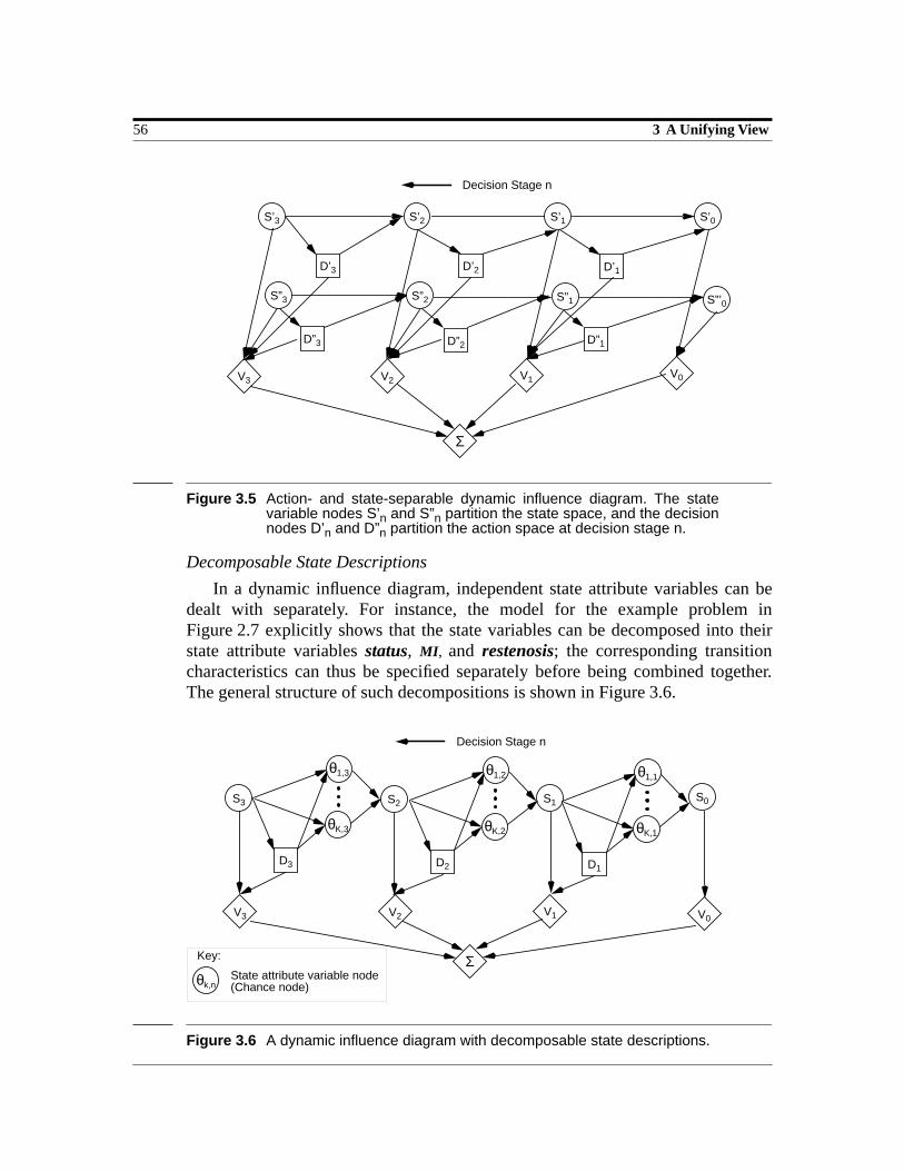
56 3 A Unifying View
Figure 3.5 Action- and state-separable dynamic influence diagram. The statevariable nodes S’n and S”n partition the state space, and the decisionnodes D’n and D”n partition the action space at decision stage n.
Decomposable State Descriptions
In a dynamic influence diagram, independent state attribute variables can bedealt with separately. For instance, the model for the example problem inFigure 2.7 explicitly shows that the state variables can be decomposed into theirstate attribute variablesstatus, MI , and restenosis; the corresponding transitioncharacteristics can thus be specified separately before being combined together.The general structure of such decompositions is shown in Figure 3.6.
Figure 3.6 A dynamic influence diagram with decomposable state descriptions.
Σ
S’3 S’0S’1S’2
D”3 D”2 D”1
V3V0V1V2
Decision Stage n
D’3 D’2 D’1
S”3 S”2 S”1 S”’0
Σ
S3 S0S1S2
θK,3
D3
V3 V0V1V2
Decision Stage n
Key:
θk,nState attribute variable node(Chance node)
θ1,3
θK,2
D2
θ1,2
θK,1
D1
θ1,1

3.3 An Analysis 57
Strategic Constraints
In general, the capabilities of a dynamic influence diagram for handling strate-gic constraints are similar to those of anSMDP. For instance, since the conven-tional solution methods for dynamic influence diagrams usually employ backwardinduction, dependent efficacies of and numeric restrictions on specific actions canbe handled only with extra state attribute variables.
Granularity of Transition Characteristics
The qualitative structure of a dynamic influence diagram is at a higher level orabstraction than a state transition diagram. Unless the action-separable organiza-tion as shown in Figure 3.5 is used, a dynamic influence diagram does not usuallyexplicate the distinct effects of different actions at a particular decision stage; suchinformation is revealed only through the corresponding conditional distributionsassociated with the state variables.
With chance nodes as part of its decision ontology, however, a dynamic influ-ence diagram can represent the transitions in more details. In addition to explicitlymodeling the state attribute variables as shown in Figure 3.6, other possible chanceevents that might influence them can also be incorporated. The structure of thevalue functions can also be explicitly depicted in these models. For a particulardecision stage, the general structure of such decompositions is shown inFigure 3.7. The ability of separately displaying these decomposed parametersallow the underlying conditional distributions to be independently assessed.
Figure 3.7 A dynamic influence diagram with chance events constituting thestate transitions and decomposed value functions. All the circles arechance nodes.
Σ
Sn-1
θK,n
Dn
Vn
Decision Stage n
θ1,nE1
EX
Sn
v1 vY

58 3 A Unifying View
Markov cycle trees and Stochastic trees
Since stochastic trees are the continuous-time analogs of Markov cycle trees, wediscuss these two techniques together. A Markov cycle tree or a stochastic tree hasthe following basic components: a set of decision nodes, a set of state nodes, a setof chance nodes, a set of conditional probability distributions associated with thechance nodes, and a set of value functions associated with the state nodes. Theconditional probability distributions in a stochastic tree is in the form of constanttransition rates.
A Markov cycle tree or stochastic tree models the consequences of a specificaction by depicting a more detailed view of the state transition diagram of theembedded Markov chain. The tree explicitly displays the possible effects of theaction, in terms of a set of chance nodes, which are implicitly captured in the tran-sition arrows of the embedded Markov chain. This correspondence is more obvi-ous if we remove all the intermediate chance nodes by conditional expectations asshown in Figure 3.8.
Figure 3.8 Comparing a) a Markov cycle tree and b) a state transition diagram.
Time Indices and Decision Horizon
The time indices are discrete in Markov cycle trees, and continuous in stochas-tic trees. The constant holding times in the former and the constant transition ratesin the latter are very strong assumptions; they cannot express situations where thetransition functions depend on the time duration since entering a state. After aPTCA, for instance, if the patient is well, it is three times more likely that he willdevelop restenosis in the next 6 months than later. This cannot be easily capturedin the models; extensions such astunnel states in the cycle trees are necessary[Sonnenberg and Beck, 1993]. Each tunnel state is a transient state that is accessi-ble in a fixed sequence; it can represent a single unit of time duration spent in theoriginal state. Figure 3.9 shows a (partial) state transition diagram for the tunnel
Well
Sick
Dead
Well
Sick
Dead
Well
Sick
Dead
Well
Sick
Dead
Well
Sick
Dead
Well
Sick
Dead
State at time t State at time t+1
a) b)

3.3 An Analysis 59
state organization in the above example. The tunnel states are represented asshaded circles. Assuming the cycle length or inter-transition interval is threemonths, the first tunnel state represents the first three months afterPTCA, the sec-ond the next there months, and the third any time, at three-month intervals, sixmonths after the treatment.
Figure 3.9 Using tunnel states to model duration dependent transitions.
Markov cycle trees can model both finite and infinite horizon problems. In sto-chastic trees, state transitions can occur at any time corresponding to some expo-nential distributions, hence they are valid only for infinite horizon problems.
Sequential Separable Decisions
In the tree-based dynamic decision models, all the states are assumed to bevalid at all times; the action associated with each Markov cycle tree or stochastictree is assumed to be applicable in all states. Since the decision ontology does notinclude decision nodes, the sequential nature of the decisions cannot be conciselyrepresented. For instance, the Markov cycle tree and the stochastic tree for theexample problem as shown in Figure 2.9 and Figure 2.10 do not include sequentialdecisions; they do not consider how backup or alternate treatments may affect thepatient’s prognosis. Such “cross-over” information can only be incorporated asadditional state attributes. The combinations of all subsequent actions and theirpossible consequences between any two successive transitions would have to bemodeled as separate states in the cycle tree. Figure 3.10 shows such an extendedMarkov cycle tree for the example problem.CABG can be performed as back-uptreatment for other actions; the implications for stayingwell after aCABG is differ-ent from stayingwell after other treatments.
PostPTCA 1
PostPTCA 2
PostPTCA
Restenosis

60 3 A Unifying View
Figure 3.10 A Markov cycle tree involving cross-over strategy with differentconsequences.
Decomposable State Descriptions
In a Markov cycle tree or a stochastic tree, state attribute variables are notgraphically depicted as chance nodes. In a Markov cycle tree, state attributes han-dling is closely related to the forward induction based solution methods. The stateattributes are defined in a set of logical or algebraic expressions asbindings associ-ated with some of the outcomes of the chance nodes. The outcomes in questionhave bindings that act like counters. For instance, in Figure 2.9, the outcomeMI ofthe chance node indicating the presence or absence ofMI has an associated bindingMI := 1. When that particular branch is traversed, the binding is set on; the statesrepresented as leaf nodes in a Markov cycle tree are determined by logical or alge-braic expressions in terms of the bindings such as:
.
As in anSMDP, state attribute variables are not handled formally by the deci-sion ontology. The backward induction based solution methods employed with sto-chastic trees also do not incorporate external devices such as bindings.
Strategic Constraints
In a Markov cycle tree or a stochastic tree, the same action, which may includeone or more diagnostic tests or treatments in the medical domain, is assumed atevery decision point. In other words, dynamic decision models employing thesetechniques can only model problems that compare the effectiveness of fixed strate-gies, but not those that determine an optimal sequence of possibly varying deci-sions.
Well after CABG
Sick
Dead
Sick
Dead
Dead
Well after CABG
Sick
Dead
Sick
DeadWell after others
Sick
Dead
Well after CABG
Well after others
Well after others
Well after CABG
CABG
No CABGMedRx
PTCA
CABG
MI+Restenosis : MI 1=( ) Restenosis 1=( )∧=

3.3 An Analysis 61
Numeric restrictions on the actions, however, can be incorporated into aMarkov cycle tree as bindings as described earlier. This avoids the extra statesneeded to incorporate such constraints. As mentioned, the bindings mechanism isspecific to forward induction based solution methods, and cannot be generalized.
Granularity of Transition Characteristics
As mentioned earlier, a Markov cycle tree or stochastic tree depicts the transi-tions in more details. In addition to the chance events constituting the transitions,the different paths or combinations of the corresponding outcomes that constitutesuch transitions are also displayed. As an example, consider the thickened linesshown in Figure 3.10. Starting at any statei from the root node, the expectation ofprobabilities associated with all the paths leading to the same state nodej consti-tutes the one-step transition function fromi to j.
Comparing to the influence diagram perspective, the tree structure is also goodfor modeling modular, asymmetric pieces of knowledge. Again with reference toFigure 3.10, the different subtree structures for thewell states indicate thatCABG isnot considered as a backup strategy if the original treatment isCABG itself. In adynamic influence diagram, such asymmetry will be encoded in the conditionaldistributions, but not revealed at the structural level.
AI Planning
The basic decision ontology of anAI planner includes a set of operators, a setof propositions or conditions, and a set of states. An operator corresponds to anaction in anSMDP, together with its applicability constraints and effects. The pre-conditions of an operator specify the subset of states in which the action is applica-ble; the postconditions of an operator specify the subset of states that are reachableafter taking the action. Together the preconditions and the postconditions deter-mine the set of transition functions associated with the action. In classicalAI plan-ning, the transition functions are deterministic; in decision-theoretic planning, thetransition functions are stochastic. A proposition corresponds to a state attribute inanSMDP. A state is a complete description of the world at a single point in time; acollection of states that describe the world at different levels of abstraction at thesame time may be defined simultaneously [Mansell, 1993]. The goal state corre-sponds to a value function in anSMDP. There is usually no explicit notion of timeexcept for sequencing order of the operators.
Time Indices and Decision Horizon
For AI planning, the time indices are usually discrete and the planning horizonis often finite.
Sequential Separable Decisions
Most AI planning research deals with complex world states and actions; it maybe very difficult or even impossible to enumerate all the states involved in a plan-ning problem. The rich and complex operator representations simplify the specifi-
qija( ) .( )

62 3 A Unifying View
cation of action applicability conditions and effects. Without additional aids suchas dependency diagrams, however, the sequential and separable nature of theactions are difficult to visualize.
Decomposable State Descriptions
In an AI planning problem, the states are usually defined in terms of a set ofpropositions. Problem formulation may or may not involve a complete enumera-tion of the state space.
Strategic Constraints
Besides the basic components described earlier,AI planning frameworks varyin their ontologies. Strategic constraints, however, are usually explicitly repre-sented. Most of the constraints involved inAI planning are either captured in theoperators or represented with external modules.e.g., temporal databases. Whilethe constraints are explicitly expressed, additional inferences may be necessary toreason about them.
Granularity of Transition Characteristics
In AI planning, the transition functions are defined in terms of the stateattributes affected by the actions. There is no further breakdown of the transitionsinto chance events that would in turn influence the state attributes.
3.3.2 Solution Methods
Solving a dynamic decision problem assumes that the problem is completely andproperly formulated in the respective framework. If more information is neededduring the process, the solution method will determine and direct the derivation ofsuch information.
Semi-Markov Decision Processes
A variety of solution methods are available forSMDPs. The most common algo-rithms are based on thevalue iteration method of the dynamic programming orBellman optimality equation. Other methods include policy iteration, linear pro-gramming,etc. Applicability of the different solution methods depends on certaincharacteristics of the problem,e.g., constant discount factor, stationary policy, andhomogeneous transition functions. A more detailed discussion on these techniquescan be found in Chapter 7 and Appendix B.
Dynamic Decision Modeling
Solving a dynamic decision model for the optimal policy is also called evaluatingthe model. Most of the evaluation algorithms are based on thevalue iterationmethod of the dynamic programming or Bellman optimality equation of semi-Markov decision processes, the discrete time Markov version of which is shown in(EQ 2’) in Section 2.3. This method is based on the notion ofbackward induction.

3.3 An Analysis 63
All possible state evolutions over time have to be explicitly enumerated in themodels, and hence considered by the evaluation algorithms. There are, however,calculations on optimal substructures that can be reused, thereby reducing theoverall amount of calculations involved.
Even then, the power of dynamic programming,i.e.,considering only the opti-mal decisions obtained so far from the future by backward induction, is actuallynot fully exploited in dynamic decision modeling. Although dynamic influencediagrams correspond to exact formulations of the dynamic programming equation[Tatman and Shachter, 1990], all the tree-based solution methods that are based onforward induction do not make use of the optimal substructure. In these lattermethods, all the possible decision consequences have to be simulated or traversedforward over time during evaluation. No reuse of optimal substructures isinvolved.
AI Planning
Solution methods inAI planning are based onheuristic search [Korf, 1987]. Thesolution algorithms are often not only concerned with finding the solution paths,but also how to cut down the search space in finding such paths. Guided by a set ofheuristics, plan generations often involve action and state spaces at multiple levelsof abstraction. The appropriate heuristics depend on the planning ontology of theframework.
3.3.3 Model Quality Metrics
To perform analysis on the model and the solution of a dynamic decision problem,we need a set of metrics to assess the quality of the model and the solution. Thequality of the solution is usually determined, with respect to domain-specificknowledge, using standard statistical techniques such as one-way and two-waysensitivity analysis. This can be done on solutions generated by all the techniquesaddressed. The quality of the model can be measured in terms of its accuracy, con-ciseness, and clarity. A model is accurate if both its structure and parametersreflect the decision situation to a “satisfactory” extent. A model is concise if it con-tains only the relevant information pertaining to the decision situation. A model isclear if it contains information that can be easily accessed by an inference processto produce “meaningful” answers. Therefore, the quality measures are not onlytheoretically meaningful, but also indicate how easily the model can be“debugged” during problem formulation and problem analysis in practice.
In this section, we briefly compare the model quality metrics for the currenttechniques. A detailed explanation of the metrics is beyond the scope of this analy-sis; references for these metrics, however, are provided. We focus on highlightingthe availability or absence of, and the similarities and differences in the metrics forthe different techniques.

64 3 A Unifying View
Semi-Markov Decision Processes
Accuracy
The fidelity of the probabilistic parameters involved in anSMDP can be mea-sured with standard statistical techniques. The accuracy of theSMDP can beassessed in terms of the mathematical properties that can be proved about it,e.g.,existence and convergence of optimal policies. Some methods that facilitate suchproofs are the certainty equivalence principle, the controllability and observabilityconditions, and the monotonicity and contraction mapping principle[Bertsekas, 1987]. The certainty equivalence principle asserts that an optimal pol-icy is unaffected by the presence of zero-mean disturbances. By analyzing theranks of the system matrices, controllability indicates if a dynamical system can becontrolled; observability determines if its variables can be inferred. If the valuefunctions manifest monotonicity or contraction mapping properties, convergenceof the corresponding solution method, and hence the existence of optimal policies,is guaranteed.
Due to its precise mathematical definitions, however, many assumptions andtransformations of the decision factors and constraints must be made to fit into theSMDP ontology. Therefore, while anSMDP supports formal analysis, such tech-niques may be difficult to apply and to understand.
Conciseness
The main difficulty in formulating aSMDP is the combinatorially increasingdimension of the state space with each relevant state attribute variable. One way toensure conciseness of the state space description is to explicitly manipulate thecombinations of state attributes with either formalcanonical forms or domain-spe-cific heuristics. Another way is to develop quantities calledsufficient statistics,which ideally would be of smaller dimension than the original state space, and yetsummarize all the essential information for problem solution and analysis[Bertsekas, 1987]. We do not know of any effective guidelines for developing suchtechniques in general.
Clarity
The clarity of anSMDP can be assessed in terms of its inferential efficiency andinformation explicitness. No formal metrics exist for this quality. In general, appli-cable inferences can be easily determined in a complete model with precise mathe-matical properties. Informational explicitness, however, cannot be easily verifieddue to the assumptions and transformations involved in problem formulation.
Dynamic Decision Modeling
Accuracy
Various metrics exist for assessing the accuracy of a dynamic decision model.Examples of these metrics include the equivalence decision class analysis fordetermining relevant chance events [Provan and Poole, 1991], the value of infor-
3.3 An Analysis 65
mation, and the “confidence” measure of the recommended decision, which com-pares the fidelity of subjective probabilities with objective relative frequencies inthe model [Willard and Critchfield, 1986] [Neapolitan, 1993]. While most of thesemetrics are applicable to any dynamic decision model type, actual implementa-tions of the metrics, and hence their ease of use, vary with different model types.This is particularly true for structural accuracy metrics. For instance, equivalencedecision class analysis is usually employed in updating dynamic influence dia-grams; the structural complexity of the tree-based decision models renders suchupdating much more difficult. In addition, some metrics are designed with specificmodel types in mind,e.g.,structural controllability and observability in influencediagrams [Chan and Shachter, 1992].
Conciseness
The structural differences also complicate the measure of conciseness amongthe dynamic decision models. The network structure of an influence diagram, forinstance, is much simpler than a branching decision tree; by allowing asymmetricoutcomes, however, a decision tree actually depicts more specific information thanan influence diagram.
Without an intuitive, uniform definition of conciseness, we usually resort todetermining theadequacy of a dynamic decision model. The information in adynamic decision model is adequate when all elements of the decision problem areclearly defined. This usually involves refining the conceptualizations of parametersassociated with the situation to a sufficient level so that a decision can be made[Clemen, 1991]. Theclarity test is a technique for measuring such adequacy[Howard, 1988].
Clarity
The clarity of a dynamic decision model can also be assessed with respect to itsinferential efficiency and informational explicitness. Again, the structural differ-ences of the decision model types render these capabilities difficult to be character-ized.
Although a dynamic influence diagram displays all the chance variables andtheir conditional dependencies in a simple network structure, the exact relationsamong the outcomes of the variables, which may be asymmetric, are encoded inthe associated conditional distributions. Careful examination of the distributionsare needed to derive the specific relations; this may hinder or complicate modeldebugging in practice.
On the other hand, a Markov cycle tree or a stochastic tree explicitly displaysall chance variable outcomes. While the specific information is easily visualizablethis way, the details may lead to a very complex tree structure. In practice, theresulting complexity is countered by adopting a few constant tree structures tomodel the consequences of all alternative actions, and using devices such as bind-ings to model the variations in information [Sonnenberg and Beck, 1993]. Unfor-

66 3 A Unifying View
tunately, this violates the constant representation requirement for transparency asdescribed in Section 3.1.1; it makes a lot of the information implicit, and hencerenders model debugging difficult.
AI Planning
Accuracy
Several formal criteria for checking the correctness of a planning model havebeen proposed [Chapman, 1987] [Lifschitz, 1986] [Rosenschein, 1981]. These cri-teria are restricted to models with some basic operator representations. Currently,there are no general techniques for ensuring the accuracy of a planning model.AI
planning languages, however, usually incorporate rich and variable representationsfor the concepts involved. For example, actions and goals represented in multiplelevels of abstraction, capabilities for handling time constraints and resourcerequirements,etc. Such expressiveness may improve model accuracy by allowingmore intuitive and more direct specification of the decision factors and constraints.
Conciseness
Given an expressive planning ontology, a planning model is usually conciselyspecified. For example, instead of enumerating all the states that an action or oper-ator is applicable in, only the relevant state attributes are specified in the precondi-tions and the effects of the operator.
Clarity
There are no formal metrics for inferential efficiency and informational explic-itness inAI planning. Since most of the decision factors and constraints are explic-itly specified in a planning model, informational explicitness can be informallyassessed. Due to the expressiveness of the planning ontology and the concisenessof the resulting model, however, more inferences may be necessary to derive use-ful information.
3.4 Summary
An analysis of theSMDPs, dynamic decision modeling, andAI planning approachesto dynamic decision making under uncertainty illuminates the following issues:
First, there is a common basis, in terms of both the task definition and the deci-sion ontology, among the three techniques. All techniques support problem formu-lation, solution, and analysis. Their decision ontologies and problem structures foraddressing the dynamic decision problems concerned in this work can also beinterpreted in terms of the mathematical definitions ofSMDPs. Each framework,however, has additional strengths and weaknesses relative to the others.
Second, there is a trade-off between model transparency and solution effi-ciency. A formal framework such asSMDP supports efficient and varied solution

3.4 Summary 67
methods, but problem formulation may require many assumptions and transforma-tions of the information involved. On the other hand, a well-structured knowledgeorganization framework inAI planning facilitates problem formulation, but prob-lem solution may involve complex inferences on such information.
Third, we have noticed that the graphical capabilities of dynamic decisionmodels add an invaluable dimension to support problem formulation and analysis.Different dynamic decision models, however, graphically depict the relevant infor-mation in different perspectives, and each perspective has its strengths and limita-tions.
We draw from these results the following conclusions:
First, a sound and flexible framework for dynamic decision making underuncertainty could result from integrating the desirable features of existing tech-niques; such an integration should build on the common basis identified.
Second, the modeling task and the solution task are not only different innature, but they also require different representational and inferential support. Avocabulary effective for supporting one task may not be adequate for the other.The weaknesses of most existing techniques arise from striving toward such acompromise.
Third, based on what we have learned in this analysis, we believe a new para-digm with multiple perspective reasoning and incremental language extensionwould supplant current approaches. Building on the basis ofSMDPs, this new para-digm would allow different representational and inferential capabilities for prob-lem formulation, solution, and analysis, and support visualization of theinformation involved in different perspectives. We introduce such a framework inthe next chapter.

68 3 A Unifying View

69
4 An IntegratedLanguage Design
To address the issues concluded from the analysis in Chapter 3, we propose a newlanguage, calledDynaMoL (for Dynamic decisionModeling Language), fordynamic decision making under uncertainty. This language design is motivated bya set of specific desiderata for dynamic decision modeling and influenced by somegeneral design principles in computer science. It distinguishes the representationaland inferential support for formulating, solving, and analyzing dynamic decisionproblems.
4.1 Desiderata of An Integrated Language
An effective language for dynamic decision making under uncertainty should pro-vide representational and inferential support for all the different tasks involved. Inparticular, it should balance the trade-off between model transparency and solutionefficiency. Such a language should have an expressive decision ontology and a for-mal basis, it should support multiple levels of abstraction and multiple perspec-tives of visualization, and it should be extensible, adaptable, and practical.
4.1.1 Expressive Decision Ontology
The decision ontology of the new language should include decision factors andconstraints common to most current frameworks; it should address, therefore, awide range of issues in typical dynamic decision problems.
The vocabulary should facilitate problem formulation. In other words, expres-siveness, succinctness, and transparency are its most important qualities. Thesequalities are determined not only by the types and varieties of the ontological com-ponents, but also by the representation and organization of the components.

70 4 An Integrated Language Design
4.1.2 Formal Theoretic Basis
The language should have a mathematical basis to support problem solution andproblem analysis. This theoretical framework should reflect the expressiveness ofthe decision ontology, but it should have simple and rigorous syntax and seman-tics. These qualities would facilitate examining and analyzing the formal proper-ties of the problem and its solutions.
4.1.3 Multiple Levels of Abstraction
During problem formulation, a user should be able to deal mainly with the relevantontological concepts, instead of the specific mathematical definitions. This indi-cates the need for a decision ontology that is flexible, “high level”, and intuitive.The language, therefore, must support reasoning at multiple levels of abstraction.
Two general types of abstraction are involved. The first type refers to the onto-logical abstraction within the high level decision ontology. Some examples areaction classes, and state and transition descriptions at different levels of details.The second type refers to the abstraction of the high level ontology from its formalrepresentation. To ensure coherent integration of a high level decision ontologyand an underlying theoretical framework, proper translations should be establishedfor each type of abstraction.
4.1.4 Multiple Perspectives of Visualization
The graphical capabilities of dynamic decision modeling should be preserved inthe new language. These capabilities facilitate modeling and analysis; they shouldbe extended to visualize the decision factors and constraints involved in multipleperspectives, and across different levels of abstraction.
Visualization in multiple perspectives reflects a common pattern in humandecision making. For instance, at one stage of problem formulation, it might beessential to consider only the possible state transitions; at another stage, it might beilluminating to estimate the uncertain effects of an action between state transitions.Again correspondences must be established among the graphical entities and rela-tions in different perspectives.
4.1.5 Extensibility
The language should be incrementally extensible. Extensions involve incorporat-ing additional language constructs for new types of decision factors and con-straints. Both the high level decision ontology and the theoretical frameworkshould be extensible. Modularity should be preserved through the translationacross multiple levels of abstraction and multiple perspectives of visualization.

4.2 Overview of Language Design 71
Given an expressive and stable theoretical framework, most of the extensionsshould be on the high level decision ontology. When additions are made to the the-oretical framework, the mathematical properties should carry over, or generalize ina straightforward manner.
4.1.6 Adaptability
The language should be systematically adaptable. Adaptation involves changes inthe organization of the language constructs; it does not necessarily affect theexpressiveness of the language. For instance, instead of incorporating asymmetricrelations in terms of the probabilities in a conditional distribution table, explicitstatements can be made about the relations, thereby making them more obvious.Again both the high level decision ontology and the theoretical framework shouldbe adaptable. Modularity should also be preserved through the translation acrossmultiple levels of abstraction and multiple perspectives of visualization.
4.1.7 Practicality
The language should support implementations that can be put into practical use. Apractical dynamic decision modeling language is modular, comprehensive, andexplicit. The components of a modular language can be implemented separatelyand then integrated directly. Implementation is thus easier and less prone to errors.The number of the implemented language features can also be incrementallyincreased. A comprehensive language is applicable for real problems. The infor-mation expressed in terms of an explicit language can be easily accessible andexamined. This would facilitate model debugging and support tools development.
4.2 Overview of Language Design
The DynaMoL design attempts to satisfy the above desiderata by integrating theexpressiveness and transparency ofAI planning languages, the graphical capabili-ties of dynamic decision models, and the concise properties and varied solutions ofSMDPs. It also incorporates the general idea of programming language design:translation of a higher level language for modeling into an object language for exe-cution.
Based on a basic decision ontology, the language has four major components: adynamic decision grammar, agraphical presentation convention, a formal mathe-matical representation, and atranslation convention. The decision grammar sup-ports problem formulation with multiple interfaces. The presentation convention,in the tradition of graphical decision models, governs parameter visualization inmultiple perspectives. The mathematical representation provides a concise formu-lation of the decision problem; it admits various solution methods, depending onthe different properties of the formal model. The translation convention guides

72 4 An Integrated Language Design
development of correspondence rules among the different perspectives and repre-sentations of the decision factors and constraints. This in turn supports modularextensions to the scope of admissible decision problems and systematic improve-ments to the efficiency of their solutions.
A dynamic decision model formulated inDynaMoL has the following parts:
• the time-horizon, denoting the time frame for the decision problem;
• a set ofvalue functions, denoting the evaluation criteria of the decision prob-lem;
• a set ofstates, denoting the possible conditions that would affect the valuefunctions;
• a set ofactions, denoting the alternative choices at each state;
• a set ofevents, denoting occurrences in the environment that might affect theevolution of the states;
• a set oftransition parameters, denoting the probabilistic and temporal charac-teristics, conditional on the actions, among the states;
• a set ofinfluence parameters, denoting the probabilistic and temporal charac-teristics, possibly conditional on the actions, among the events and the states;
• a set ofdeclaratory constraints, such as the valid conditions of and logicalrelationships among the states, events, transition parameters, and influenceparameters; and
• a set ofstrategic constraints, such as the valid durations for certain actions, thenumber of times an action can be applied, the valid ordering of a set of actions,and the required duration between successive actions.
The initial DynaMoL design consists of a basic set of model components. Inparticular, the constraint definitions are minimal. The ontology is extended byincrementally incorporating individual translators or correspondence rules.
4.3 DynaMoL: The Language
The syntax of the language is defined by the dynamic decision grammar and thegraphical presentation convention. The semantics is defined by the mathematicalrepresentation of anSMDP and the translation that bridges the grammar, the presen-tation, and the mathematical representation of the decision factors and constraints.This section summarizes the decision ontology and the features of the languagecomponents; Chapters 6 and 7 discuss the definitions in more details.

4.3 DynaMoL: The Language 73
4.3.1 Basic Decision Ontology
We adopt a knowledge formalization approach similar to first-order predicate cal-culus (FOPC), as presented in [Genesereth and Nilsson, 1987]. InDynaMoL, acon-ceptualization of a decision situation includes the relevant decision parameters andthe interrelationships among them. Formally, a conceptualization consists of auni-verse of discourse, a functional basis set, and arelational basis set. The universeof discourse is the set of decision parameters about which knowledge is beingexpressed. Various functions and relations can be defined among these parameters.The functional basis set is the set of relevant functions in the universe of discourse.The relational basis set is the set of relevant relations in the universe of discourse.In the example problem introduced in Section 2.2, the universe of discourseincludes the actionsPTCA, CABG, andMedRx, and their consequences in terms ofstatus,MI, and restenosis. The functional basis set includes the probability func-tions and value functions defined. The relational basis set includes the probabilisticand temporal dependences.
Based on the conceptualization, we define the expressions inDynaMoL interms of the following components:basic concepts, variable concepts, functions,relations, andconstraints. These concepts are analogous to the constant symbols,variable symbols, function symbols, relation symbols, and sentences or well-formed formulas inFOPC. Many of theDynaMoL concepts, however, also haveprobabilistic interpretations. All of the variable concepts, for instance, also corre-spond to the random variables in probability theory. Moreover, both deterministicand probabilistic relations are involved.
Basic Concepts
A basic concept is a description of the world, within the universe of discourse, at asingle point in time. There are three types of basic concepts:events, actions, andstates.
Event
An event is a partial description of the world at a single point in time. It corre-sponds to a proposition or atomic sentence inFOPC. In particular, it describes anoccurrence or a lack of occurrence of a phenomenon. Both “presence ofMI” and“absence ofMI” are events. In a clinical decision situation, an event representseither an occurrence or a lack of a physical or physiological condition of one ormore patients,e.g., “restenosis occurred” and “restenosis did not occur.”
Action
An action is a special type of events which involves an actor. The actor can bethe decision maker concerned, in which the action is controlled; the actor can alsobe unknown and the action is subject to chance, in which case the action isembed-ded. In a clinical decision situation, relevant actions include different tests andtreatments, and their combinations,e.g., “revascularization performed” and “no

74 4 An Integrated Language Design
revascularization performed.” The effects of an action are expressed in terms ofevents. A complication of the actionPTCA is the event “presence ofMI.”
State
A state is a complete description of the world at a single point in time. Thestate description comprises a set of events or proposition as defined above. Forinstance, the statewell in the example problem is defined in terms of the events: status = alive, MI = absence,restenosis = absence. Every state has an associ-atedvalue, indicating the desirability of being in that state.
Variable Concepts
A variable concept corresponds to a random variable in probability theory. It rep-resents the uncertainty about the world, as described by the basic concepts, at asingle time point. We only consider discrete variables in this work.
a) Chance Variable
A chance variable corresponds to a chance node in a decision model. It hasseveral possible outcomes or values; the outcomes can be events or states. Eachpossible outcome occurs only by chance and cannot be explicitly chosen. There arethree types of chance variables: event variables, state attribute variables, and statevariables.
Event Variable:
The outcomes of an event variable are events. An event variable usually repre-sents a possible consequence of an action. In particular, it can capture an observ-able or unobservable phenomenon that directly or indirectly describe the states.
State Attribute Variable:
A state attribute variable is a special kind of event variables; it represents acharacteristic or property directly relevant to describing the states. The outcomesof a state attribute variable are events. Given a set of such variables, a state is usu-ally defined in terms of the Cartesian product of their outcomes. For instance, inthe example problem, all the event variables involved:status, MI , andrestenosis,are state attribute variables. The state attribute variablestatus has outcomesaliveanddead, MI has outcomespresence ofMI andabsence ofMI, andrestenosis hasoutcomespresence of restenosis andabsence of restenosis.
State Variable
A state variable represents the uncertainty about the actual state that the worldis in at a single point in time. It corresponds to a state space in anSMDP and a statevariable node in a dynamic influence diagram at that time point or decision stage.All of the outcomes of a state variable are states.

4.3 DynaMoL: The Language 75
b) Action Variable
An action variable denotes a decision or choice point at a single point in time;it corresponds to part or all of theaction space in anSMDP or a decision node in adynamic influence diagram at that time point or decision stage. An action variablehas several possiblealternatives, which are actions. Any alternative action can beexplicitly controlled or chosen as the decision.
c) Function Variable
A function variable denotes the value function or desirability measure struc-ture at a single time point. It corresponds to a value node in a dynamic influencediagram at that time point or decision stage. Each outcome of the function variableis a number, a table, or a function representing the value or desirability of a stategiven an action. In other words, the outcomes of such a variable are determined bythe Cartesian product or other functional combination of the outcomes of a statevariable and those of an action variable.
Relations
The basicrelations among the concepts are probabilistic dependences and tempo-ral dependences.
Probabilistic Dependences
A probabilistic dependence relation between two concepts corresponds to theconditional dependence notion in probability theory. Such a relation indicates aconcept is conditionally dependent on another. The direction of a probabilisticdependence relation reflects the definition of the underlying conditional depen-dence; it has no temporal implication. The special class of probabilistic depen-dence among the states are called transitions.
Temporal Dependences
A temporal dependence relation between two concepts indicates that one tem-porally precedes another; it has no causal implication.
Functions
The basicfunctions defined over the concepts and the relations are probabilityfunctions and value functions.
Probability Function
A probability function is either aPMF or aCDF.
Value Function
A value function measures the desirability of a state. Such a measure may havedifferent dimensions, e.g., monetary cost and life expectancy, and are usually con-ditional on an action.

76 4 An Integrated Language Design
Constraints
The constraints are meta-level descriptive or prescriptive conditions imposed onthe concepts, the relations, and the functions as defined above. They correspond tothe logical sentences and quantification sentences inFOPC. Some examples are theapplicability of actions with respect to the states or time or both, and the validity ofstates and events with respect to each other or time or both. For instance, given astate spaceS, the following constraint specifies that the actionPTCA is applicablein all states:
The relationApplicable, of course, will be properly interpreted by the model con-structor and solution algorithm to impose the constraint.
4.3.2 Dynamic Decision Grammar
The dynamic decision grammar forDynaMoL is anabstract grammar. Followingthe convention in [Meyer, 1990], this grammar contains the following compo-nents:
• A finite set of names ofconstructs;
• A finite set of productions, each associated with a construct.
An example of a production that defines the construct “model” is as follows:
Each construct describes the structure of a set of objects, called thespecimensof the construct. The construct is the (syntactic)type of its specimens. In the aboveexample, an object with the typeModel has five parts:name (with type Identifier),contexts (with typeContext-list),... etc. The constructs/types appearing on the right-hand side of the above definition are similarly defined by different productions. Aset of primitive constructs/types are assumed,e.g, String, Cumulative DistributionFunction, etc.
There are some fixed ways in which the structure of a construct can be speci-fied. The above example shows an “aggregate” production,i.e., the construct hasspecimens comprising a fixed number of components. Other types of productionsinclude:
Model → name: Identifier;
contexts: Context-list;
definitions: Definition-list;
constraints: Constraint-list;
solution: Optimality-policy
s S Applicable PTCA s,( ),∈∀

4.3 DynaMoL: The Language 77
“Choice” productions,e.g., the time duration in the decision horizon can befinite or infinite:
“List” productions,e.g., the state-space of the decision problem consists of oneor more states:
The DynaMoL grammar defines the structure of a dynamic decision model interms of its components; the structures of these components are recursivelydefined in a similar manner. The grammar specifies the information required tobuild a model. On the other hand, there can be many ways to manipulate suchinformation. In other words, the abstract grammar can support different interfaceimplementations. For example, an object of typeState-space may be specified in 3different ways:
• Text command interface: Type “state-space state-1 state-2 state-3” to com-mand-prompt.
• Graphical interface: Draw three state-nodes labeled “state-1,” “state-2,” “state-3” in the display window.
• Routine or code interface: Type “(define-state-space 'state-1 'state-2 'state-3)”to the Common Lisp prompt.
The complete grammar for the current version ofDynaMoL is given in Appen-dix A.
4.3.3 Graphical Presentation Convention
The graphical presentation convention inDynaMoL prescribes how the decisionfactors and constraints expressible in the grammar are displayed; it determineshow the same information can be visualized in multiple perspectives. Two generalperspectives or views are defined:transition view andinfluence view. The currentpresentation definitions adhere to the established graphical representations such asMarkov state transition diagrams and dynamic influence diagrams. These defini-tions, however, can be changed easily as long as the graphical components consis-tently correspond to the dynamic decision grammar constructs. Additionalperspectives such as partial decision tree view, information flow view, and two-dimensional Cartesian plots, can also be incorporated when appropriate.
Transition View
The transition view corresponds directly to the Markov state transition diagram.Given an action, the transition view depicts the possible state transitions, as shownin Figure 4.1.
Time-duration → |
State-space → State+
ℑ+ 0 ∪ ∞

78 4 An Integrated Language Design
Figure 4.1 Transition view for an action. The nodes denote the states; the linksdenote the possible transitions from one state to another.
Influence View
Given an action, the influence view depicts the possible event variables that affectthe transitions from one state to another, as shown in Figure 4.2.
Figure 4.2 Influence view for an action. The index “n” indicates the relevantdecision stage. The shaded nodes depict the states, the clear nodesthe possible event variables that affect the state transitions, and thelinks the probabilistic dependences.
4.3.4 Mathematical Representation
The mathematical representation of a dynamic decision model formulated inDynaMoL is anSMDP as described in Section 2.3. All the solution methods forSMDPs can be used to derive an optimal policy for the dynamic decision model for-mulated inDynaMoL. The mathematical representation will also support formalanalysis on the model and its solutions.
STATE-1
STATE-2STATE-3
STATE-4
STATE-1-n STATE-1
STATE-2-n STATE-2
STATE-3-n STATE-3
STATE-4-n STATE-4
EVENT-3
EVENT-1
EVENT-2
EVENT-4

4.3 DynaMoL: The Language 79
4.3.5 Translation Convention
Two general types of translation are involved:inter-level translation andinter-per-spective translation. In inter-level translation, a dynamic decision model specifiedin the dynamic decision grammar inDynaMoL is automatically translated into anSMDP. The model specification may involve more constructs than those defining anSMDP. A set of translators or correspondence rules are employed to bridge the con-structs of the dynamic decision grammar and the graphical presentation conven-tion with the definitions of theSMDP. The general idea, as illustrated in Figure 4.3,is to map a construct or a set of constructs in the grammar to an entity or relation inthe mathematical representation.
Figure 4.3 Inter-level translation by mapping. Each arrow type indicates atransformation function or correspondence rule.
Problem formulation and analysis inDynaMoL involve specifying and examin-ing the decision factors and constraints in multiple perspectives. The different per-spectives may facilitate expressing the same knowledge in different ways. Forinstance, a state transition can be specified either directly in terms of thePMF orCDF of a one-step transition function, or indirectly as several constituent eventvariables and the associated conditional probability distributions. Inter-perspectivetranslation, therefore, establishes proper correspondence among the different rep-resentation or organization formats. Since the same information is involved, inter-level translation can then be defined in terms of any covering set of organizationformats among the different perspectives. Figure 4.4 illustrates the idea of inter-perspective translation.
Dynamic Decision Model in Decision Grammar Mathematical Representation
state
state-space-at-n
transition
state-1
state-variable-at-n
event-variable-1
transition-1-2
state-2
influence-1-1
γsγs
γt
γsv
influence-1-2
γi

80 4 An Integrated Language Design
Figure 4.4 Inter-perspective translation by mapping. Each arrow type indicates atransformation function or correspondence rule. Directions of thearrows indicate directions of translation.
4.4 DYNAMO: A Prototype Implementation
Figure 4.5 shows the system architecture of a prototype implementation ofDynaMoL. The system, calledDYNAMO1, is implemented in Lucid Common Lispon a Sun SparcStation, with theGARNET graphics package [Myers et al., 1990]. Itincludes a graphical user interface that allows interactive model specification. Thespecification can be strictly text-based, or aided by the available graphical presen-tations of the decision factors and constraints. Figure 4.6 shows the interface of thecurrent version ofDYNAMO. Only a subset of the dynamic decision grammar isincluded in this implementation; the solution method supported is value iteration.
Figure 4.5 The system architecture of DYNAMO: a prototype implementation ofDynaMoL. The blocks indicate system components; the arrowsindicate information inflows.
1. This system has no association with the DYNAMO simulation language[Pugh, 1970].
Influence View Transition View
state
state-space-at-n
transition
state-1
state-variable-at-n
event-variable-1
state-2
influence-1-1
γsγs
γsv/γss
influence-1-2
γi
Graphical Interface
Translator SolverBase-Language

4.4 DYNAMO: A Prototype Implementation 81
Figure 4.6 The DYNAMO interface.
DYNAMO V 0.5
File Edit Model Solution Analysis
MODEL-NAME: New-Model
PATHNAME: ./New.sbin
DISCOUNT-FACTOR: 1.0
VALUE-FUNCTION-UNIT: QALE
TIME-UNIT: YearTIME-DURATION: 12
TIME-HORIZON: Finite Transition-View
Influence-View
Welcome to DYNAMO! (make-action ’ACTION-A) #<Action ACTION-A> (make-action ’ACTION-B) #<Action ACTION-B> (define-action-space :static :actions ACTION-A ACTION-B) #<Simple-Array T (1 1) 20E2006>
Transition View
View Edit
ACTION: ACTION-ARELATIONS-LIFESPAN: AllENTITIES-LIFESPAN: All
State Transition Double-transition
WELL ILL
DEAD
Influence View
View Edit
ACTION: ACTION-ARELATIONS-LIFESPAN: AllENTITIES-LIFESPAN: All
Event Decision Value Influence
WELL-n WELL
ILL-n ILL
DEAD-n DEAD
Disease-1
Disease-2

82 4 An Integrated Language Design

83
5 A Case Study
To facilitate discussion and evaluation of decision making inDynaMoL, we haveconducted a comprehensive case study based on an actual decision situation inmedicine1. This chapter introduces the background, the problems and the assump-tions involved. Details of the case study are discussed in Chapters 6 and 7. A com-plete description of the model data and solution results is given in Appendix C.
5.1 Management of Paroxysmal Atrial Fibrillation
Atrial fibrillation (AF) is a kind of cardiac arrhythmia or abnormal heartbeat. Itmeans irregular and rapid randomized contractions of the atria working indepen-dently of the ventricles. It has two undesirable side-effects: 1) it causes hemody-namic deterioration at very slow or very rapid heart rates and a loss of atrialmechanical contraction; and 2) blood clots can collect in the fibrillating atrium thatmay subsequently embolize,i.e., become material masses present in the bloodstream [Fishman et al., 1985]. Embolization is dangerous because it blocks bloodflow to the target organs and may lead to strokes, renal failure, gangrene of thelegs,etc.
AF can occur in paroxysms,i.e., sudden, periodic episodes. Both the frequencyand the length of theAF episodes usually increase with time; constant fibrillationoften develops eventually.
1. This case study is based on a consult case for the Division of Clinical DecisionMaking at the Tufts-New England Medical Center. Dr. Charles A. Ellis is in-charge of this consult; he has kindly provided the background medical knowledgeand shared the dynamic decision modeling expertise involved in the case study.The original consult was done in a Markov cycle tree framework.

84 5 A Case Study
Management ofAF involves antiarrhythmic agents to control the heart ratesand to restore normal sinus rhythm. Because of the risk of embolization, anticoag-ulants such as warfarin and aspirin are often used to prevent blood clot formationin the atria. The treatments, however, have undesirable side-effects of their own. Inparticular, a commonly used antiarrhythmic agent, Quinidine, increases the risk ofsudden death; an anticoagulant may cause excessive bleeding, which in turn maylead to strokes or death.
5.2 Case Description and Clinical Questions
The patient is a 52 year old white male with a history of paroxysmalAF. He hasbeen on warfarin, an anticoagulant, for about 10 years, and on Quinidine, an anti-arrhythmic agent, for a shorter period. His arrhythmic attacks are asymptomatic,and of unknown frequency and duration. Since mid-1990, several episodes ofAF
have been detected, and the level of quinidine prescribed has been steadily raisedaccordingly. Each prescription adjustment has been able to bring him back to nor-mal sinus rhythm(NSR), i.e., out of arrhythmia. The patient is recently diagnosedas being diabetic and put on diabetic medication. He also has mild hypertensionand a slightly diminished ejection fraction. All these three factors are associatedwith increased risk of embolization.
The clinical questions to be addressed is as follows:
Problem 1: Quinidine decreases the proportion of time that the patient spends inAF. Does this decrease his risk of embolic complications enough to justify theincreased risk of sudden death?
Problem 2: What is the optimal course of treatment in the next five years, takinginto account the varying relative risk of bleeding for warfarin with respect to theduration of treatment?
5.3 Assumptions
AF is the only relevant condition targeted in the dynamic decision problems. Thepatient’s diabetes, hypertension, and diminished ejection fraction are not affectedby theAF therapy; these conditions, however, markedly influence the likelihoodsof various therapeutic consequences.
The actions involved are Quinidine and warfarin. Quinidine is strictly an exter-nally controlled action. Warfarin, on the other hand, can be initiated or prohibitedin accordance with certain observable events. The effects of the actions may recurand also vary in duration.

5.4 Assessment Objectives 85
Effects of Quinidine
Quinidine decreases the likelihood ofAF. Its most undesirable side-effect is toincrease the risk of sudden cardiac death.
Effects of Warfarin
Warfarin decreases the risk of thromboembolism or embolization of blood clots. Athromboembolic event may be transient or result in a stroke. The undesirable side-effects of warfarin include cerebral hemorrhage,i.e., bleeding in the brain, andgastrointestinal bleeding,i.e., bleeding in the stomach and the intestines. All theseconsequences may be fatal.
The relative risk ratio compares the rate at which an event occurs given and notgiven an action [Wong et al., 1990]. The relative risk of bleeding for warfarin, withrespect to the duration of treatment, is assumed to be constant in the first problem,and varying in the second problem.
Initiation and Prohibition of Warfarin
Occurrence of a thromboembolic event will mandate initiation of warfarin if thepatient is inAF, and if warfarin is not prohibited. Once warfarin is initiated, it willnot be stopped unless there are contra-indications.
Occurrence of a bleeding event, either cerebral or gastrointestinal, will man-date discontinuation of warfarin. This will also prohibit warfarin from being pre-scribed in the future.
5.4 Assessment Objectives
The case study aims to illuminate the theoretical and practical capabilities and lim-itations of theDynaMoL framework. To show thatDynaMoL can handle an actualdynamic decision problem in medicine, we adhere closely to the original clinicalconsult in addressing the first clinical question. To show thatDynaMoL offers addi-tional flexibility to existing frameworks, we focus on illustrating the ontologicaland computational features involved in addressing the second clinical question; theclinical significance of the data and assumptions adopted in this latter problem areless important.
We informally assess the effectiveness of modeling and solving the twodynamic decision problems with respect to three criteria. First, we demonstratehow the relevant decision factors and constraints can be expressed in theDynaMoLontology. Second, we compare the solutions to the results of the actual clinicalconsult or the clinical judgment of domain experts or both. Third, we examinesensitivity analysis results on the solutions to ensure reasonable behavior of theparameters involved.

86 5 A Case Study
For ease of exposition, we formulate the two dynamic decision problems interms of a single dynamic decision model with two sets of slightly different numer-ical parameters. Chapter 6 details how we construct the dynamic decision modeland translate it into its mathematical representation. Chapter 7 describes the solu-tion methods involved and the sensitivity analyses supported.

87
6 Dynamic DecisionModel Formulation
As mentioned in Chapter 3, dynamic decision making under uncertainty is an iter-ative process; it involves interleaving and repeating steps of problem formulation,solution, and analysis. Problem formulation is mainly a modeling process; prob-lem solution is a computational process. Analyses on the model and its solutionsbridge and improve the modeling and the computational results.
In this chapter, we examine problem formulation inDynaMoL. With the aid ofthe DYNAMO system interface, we describe in detail the language syntax andsemantics in terms of the modeling tasks they support. To highlight the languagefeatures, we also explain how such tasks are handled in other dynamic decisionmodeling frameworks when appropriate.
In the following discussion, details of the case study introduced in Chapter 5serve mainly as examples to illustrate the different modeling tasks. The choice ofthe modeling assumptions are less essential.
6.1 Dynamic Decision Modeling in DynaMoL
Problem formulation inDynaMoL involves constructing a dynamic decision modeland translating it into its mathematical representation. The model captures the rele-vant decision factors and constraints for solving a dynamic decision problem. Inthe programming language analogy, a dynamic decision model is a program writ-ten inDynaMoL that can be compiled or interpreted into its mathematical represen-tation. Such a program can also be viewed as anobject representing the dynamicdecision problem in the object-oriented programming paradigm. Computationalmethods are then applied to the model and its mathematical representation to pro-duce solutions for and answer queries about the problem.

88 6 Dynamic Decision Model Formulation
A dynamic decision model inDynaMoL is a well-formed or complete modelwhen it corresponds to a well-formedSMDP with an optimality criterion. Somemodel constructs directly correspond to the underlying mathematical definitions,others need to be translated. The default optimality criterion is finite horizon dis-counted total expected value.
Definition 1 (Dynamic Decision Model) A dynamic decision model M inDynaMoL is an 8-tuple together with an optimalitycriterion, where:
T is the time-index set or decision horizon;
A is the action space;
S is the state space;
E is the event-variable space;
ΩE is the set of events or outcomes of the event variables;
Ξ is the set of transitions;
Ψ is the set of influences;
ς is the set of value functions;
Κ is the set of constraints; and
G is the set of translators.
6.2 Model Construction
Dynamic decision model construction inDynaMoL typically comprises the follow-ing tasks:
1. Specify a dynamic decision problem type, its duration, and its optimality andevaluation criteria.
2. Define the alternative actions and the states involved.
3. Conditional on each action, specify the possible transitions among the statesand the values achievable in the states.
4. When such transitions and values are unobservable or difficult to be directlyassessed, specify the possible event variables and their relations that constitutethe transitions.
5. Impose relevant constraints among the decision factors when appropriate.
Besides a natural way to begin model construction, there is no strict order onthe tasks involved. The specifications and definitions may and often change in themodeling process. A major challenge for the modeling language, therefore, is toprovide adequate and direct support for the changes. InDynaMoL, such support isprovided by the dynamic decision grammar, the graphical presentation convention,and their respective interfaces.
T A S E ΩE Ξ Ψ ς K Γ, , , , , , , , ,⟨ ⟩

6.2 Model Construction 89
6.2.1 Basic Problem Characterization
The basic characteristics of a dynamic decision problem are determined by theproblem type, thedecision horizon, and theevaluation criterion. The problem typeindicates the nature of the decisions involved. The decision horizon determines thetime frame in which the decisions are relevant. The evaluation criterion specifiesthe objective or goal of the decisions; multiple criteria may sometimes beinvolved.
Problem Type
Two types of dynamic decision problems are supported byDynaMoL: optimizationproblems anddiscrimination problems with respect to some objective or evalua-tion criterion. An optimization problem is solved by constructing an optimal pol-icy:
where is an optimizing function from the state spaceS to theaction spaceA at timet with respect to the time index setT.
An optimization problem compares the independent effects of actions; theproblem solution answers the question: Ateach decision stage, what is the bestalternative action to take?
Contrarily, a discrimination problem is solved by choosing the best policy:
from a predetermined set of single-action stationary policies ,i.e., policieswhich involve a single action over the entire decision horizon, such that
where , is a function from the state spaceS to an optimizingaction .
There are two types of discrimination problems. The first type also comparesthe independent effects of actions; the problem solution answers the question: Forall decision stages, what is the best alternative action to take? The second typedelineatesstrategies or combinations of actions with dependent effects. It allowsall the possible consequences of some actions to be considered, instead of only theeffects of the optimal action. This formulation designates a single action as exter-nally controlled in a strategy, and incorporates the application pattern of all theother actions, called theembedded actions, in the state descriptions. To solve theproblem, an explicit enumeration of the policies associating each controlled actionand all possible combinations of the embedded actions is necessary. The problemsolution answers the question: Forall decision stages, taking into account the
π* µ0* µ1
* µ2* µ3
* … , , , ,=
µt* : S A t T∈;→
π* πa*=
πa
πa* µa* µa* µa* µa* … , , , ,=
µa* : S a* a* A∈;→a*

90 6 Dynamic Decision Model Formulation
effects of the controlled and embedded actions, what is the best alternative strategyto take?
In clinical decision making, determining the best course of diagnostic tests andtreatments are optimization problems, while comparing the efficacies of diagnostictests and treatments are discrimination problems. The first dynamic decision prob-lem in the case study is formulated as a discrimination problem.The problem is todetermine the net effects of the antiarrhymic agent Quinidine on a patient who ison the anticoagulant warfarin; Quinidine is a controlled action, warfarin an embed-ded action. As mentioned in Section 5.3, warfarin is never stopped once it isadministered, unless there are contra-indications for it. Similarly, warfarin is neveradministered again once it is stopped. Four strategies are to be discriminated:
1. Strategy “None”: Start without any drug, with warfarin administered andstopped as necessary;
2. Strategy “Warfarin”: Start with warfarin, which can be stopped when neces-sary;
3. Strategy “Quinidine”: Start with Quinidine, with warfarin administered andstopped as necessary; and
4. Strategy “Both”: Start with both Quinidine and warfarin, with warfarin stoppedwhen necessary.
The second dynamic decision problem in the case study is formulated as anoptimization problem. The problem is to determine a course of optimal initialaction, e.g., start with or without warfarin or Quinidine or both, with strategicimplications as defined above.
Other dynamic decision modeling frameworks support formulation of optimi-zation and discrimination problems to different extents. Dynamic influence dia-grams support direct formulation of both optimization and discriminationproblems. Without augmenting computational structures such as bindings or flags,and assumptions on the solution methods, both Markov cycle trees and stochastictrees only support direct formulation of discrimination problems. The tree-basedtechniques do not support direct formulation of optimization problems becausethey do not allow decisions to be made in stages; a decision is made only at thefinal stage by comparing the objective values for the individual decision alterna-tives over the entire decision horizon.
Decision Horizon
The decision horizon can be finite or infinite. A finite hori-zon model with a long duration and small time units may be approximated as aninfinite horizon model. We shall discuss more about the conditions under whichsuch an approximation is feasible in Chapter 7.
Clinical decision problems usually involve finite decision horizons because thepatient’s life-expectancy is finite. Long-term decision horizons project the deci-
T 0 1 2 3 …, , , , =

6.2 Model Construction 91
sions over an approximation of the patient’s lifetime; short-term decision horizonsconsider the best course of action in the immediate future,e.g., in the next fiveyears. In the case study, we assume a long-term decision horizon of 50 years or600 months for the first dynamic decision problem, and a short-term decision hori-zon of 5 years or 60 months for the second.
Evaluation Criterion
The evaluation criterion can be in any unit of interest,e.g., life expectancy, mone-tary cost, and cost-benefit ratio; it is defined by one or more sets of value functions.More than one evaluation criterion may be involved. We may be interested todetermine the quality-adjusted life expectancy of a patient, as well as the monetarycost incurred by his illness in the next five years. As in all other dynamic decisionmodeling frameworks, the value functions are assumed to be linear and additive.We will formally define the value functions in Section 6.2.7. The evaluation crite-rion for the case study problem is quality-adjusted life expectancy.
Figure 6.1 shows part of theDYNAMO interface that specifies some of the basicproblem characteristics for the case study.
Figure 6.1 Basic problem characteristics of the case study (partial).
6.2.2 Action Space Definition
Theaction space denotes the set of actions to be consid-ered in the dynamic decision problem.DynaMoL currently assumes astatic actionspace,i.e., the action space remains unchanged over the entire decision horizon.We explain how this assumption can be relaxed in Chapter 8.
The action space of an optimization problem model consists of the individualactions. The action space of a discrimination problem model consists of the con-trolled actions of the relevant strategies; the most basic strategies involve only thecontrolled actions with no additional embedded actions. Note that the word actionindicates a single unit of behavior. An action may actually involve more than oneactivity, e.g., administer two drugs and perform two diagnostic tests; the constitu-ent activities in an action are assumed to be simultaneous and constant at everydecision stage.
In the case study, the action space consists of the two controlled actions for thestrategies involved: . The effects of the embedded
MODEL-NAME: Case-Study-Model
PATHNAME: ~/Case-Study.sbin
DISCOUNT-FACTOR: 1.0
VALUE-FUNCTION-UNIT: QALE
TIME-UNIT: MonthTIME-DURATION: 600
TIME-HORIZON: Finite
A a1 a2 … a A, , , =
A NoDrug Quinidine, =

92 6 Dynamic Decision Model Formulation
action warfarin with or without Quinidine are expressed in the state descriptions,as described in the next subsection, and can be read off directly.
6.2.3 State Space Definition
Thestate space denotes the set of states in which the con-trolled actions can take place.DynaMoL currently also assumes astatic state space,i.e., the state space remains unchanged over the entire decision horizon. Weexplain how this assumption can be relaxed in Chapter 8.
The states are defined in terms of a set ofstate attribute variables; these vari-ables denote the different characteristics that constitute and distinguish the states.There are three types of state attribute variables. The first type affects the valuefunctions,e.g., quality-adjusted life expectancy of a patient depends on whether hehas normal sinus rhythm or atrial fibrillation. The second type indicates the eligi-bility of one or more actions,e.g., warfarin is applicable only in a state with noprevious contra-indication for anticoagulation. The third type reflects the status ofone or more embedded actions,e.g., whether warfarin is administered in a statewhen Quinidine is considered.
The states are usually defined as the Cartesian product of the outcomes of thestate attribute variables. This definition, however, leads to many redundant orinvalid state descriptions in practice. For instance, the most common state attributeinvolved in clinical decision making is whether the patient is alive or dead; if thepatient is dead, all other state attributes are irrelevant, and the state space size canbe cut in half. There are many ways in which the state space can be reduced in size.Most of them, however, involve domain specific heuristics. In general, such heu-ristics can be expressed in terms of the declaratory constraints to be described inSection 6.2.8.
The relevant state attribute variables and their possible outcomes in the casestudy are shown in Table 6.1.Sinus rhythm indicates heartbeat pattern.Cerebralvascular accident indicates obstruction of blood flow to the brain, which mayresult in a stroke or temporary weakness. These two state attributes affect the valuefunctions.Warfarin eligibility affects the applicability of the action warfarin.War-farin statusreflects the status of the embedded action warfarin.
The states are defined in terms of the Cartesian product of the outcomes of theabove four state attribute variables. A complete listing of the states can be found inAppendix C. We employ a simple heuristic to reduce the size of the state space:Since warfarin will not be administered when it is not eligible, we eliminate thatcombination in the resulting states.
S s1 s2 … s S, , , =

6.2 Model Construction 93
In dynamic influence diagrams, the state attribute variables are represented aschance nodes directly influencing the value nodes; the implicit state descriptions,therefore, are strict Cartesian product of the outcomes of these chance nodes. InMarkov cycle trees and stochastic trees, state attribute variables are not captured inthe bindings; state space definition in these frameworks often involves logicalcombinations of the relevant bindings.
6.2.4 State Transition Specification
Conditional on each controlled action, a set of possibletransitions is defined among the states.
Definition 2 (Transition) A transition relation between anytwo states , given an action at time , denotes the accessibilityof j from i given a at t. The nature of this accessibility is characterized by a one-step transition function withPMF and CDF as defined for anSMDP in Section 2.3.
Recall that a transition function is a joint probability distribution governing thetwo dimensions of a transition: destination of the transition and time remaining orduration before the transition; temporal precedence is imposed in determining thedestination. As described in Section 2.3, one way to calculate the transition func-tions is by multiplying the eventual transition probability and the hold-ing-time PMF or CDF . Another way to calculate the transitionfunction is by multiplying the conditional transition probability and thewaiting-time PMF or CDF . States with no out transitions arecalledabsorbing states.
Table 6.1 State attribute variables and their outcomes for the case study
State Attribute Variable OutcomesStatus Alive (Alive)
Dead (Dead)
Sinus rhythm Normal sinus rhythm (NSR)Atrial Fibrillation (AF)
Warfarin eligibility Warfarin-OK (War-OK)Warfarin-Not-OK (War-No)
Warfarin status Warfarin-On (War-On)Warfarin-Off (War-Off)
Cerebral vascular accident None (None)Transient ischemic attack (TIA)Stroke (Stroke)
Ξ ξ a i j t, , ,( ) i j, S a A t T∈,∈ ,∈=
ξ A S S T×××⊆i j, S∈ a A∈ t T∈
qija( ) .( ) Qij
a( ) .( )
Pija( ) .( )
hija( ) .( ) Hij
a( ) .( )pij
a( ) .( )wi
a( ) .( ) Wia( ) .( )

94 6 Dynamic Decision Model Formulation
The possible transitions may be estimated before the transition functions areexactly defined. For instance, there is a transition from every state to thedead state.Similarly, once a patient is ineligible for warfarin treatment, he should not be ableto make a transition to a state where warfarin is on. InDynaMoL, the transitionview supports graphical presentation of the Markov state transition diagram. Tran-sition functions can be specified directly on the links representing the transitions.
A transition view of the states and the possible transitions for the action Quini-dine is shown in Figure 6.2. For ease of exposition, it is an abstract or abbreviatedview in that only two state attributes that affect the transition patterns:warfarineligibility andwarfarin status are included in the state descriptions. The actualstate transition diagram has all the states with the displayed state attributes con-nected to each other in a similar manner.
Figure 6.2 An abbreviated transition view for action Quinidine in case study.
All current dynamic decision modeling frameworks do not support visualiza-tion of the state transitions in the transition view manner.
6.2.5 Event Variable Space Definition
At times it is difficult to specify the transition functions directly, especially whenthe action effects are partially observable or unobservable. Such effects are mod-eled inDynaMoL as event variables and their associated relations among the states.For each controlled action , itsaction-specific event variable space
denotes the set of event variables that constitute itseffects. Theevent variable space denotes the set of all event vari-
Transition View
View Edit
ACTION: QUINIDINERELATIONS-LIFESPAN: AllENTITIES-LIFESPAN: All
State Transition Double-transition
WARFARIN-ONWARFARIN-OFF
DEAD
WARFARIN-NOT-ELIGIBLE
a A∈Ea e1 e2 … e Ea
, , , =E Eaa A∈∪=

6.2 Model Construction 95
ables for all the actions. Each event variablee has an associated eventor outcomespace , which denotes the set of possible outcomesfor e. Theaction-specific event space and theoverall event space are sim-ilarly defined.
In DynaMoL, the action-specific event variable space can be different; theevent variable space however, is currently assumed to be static over time. In otherwords, the event variables associated with different actions may be different, butthe same set of event variables are associated with each action over all decisionstages. In the case study, the action-specific event variable spaces for the controlledactions NoDrug and Quinidine are assumed to be the same; the relevant event vari-ables indicate the presence or absence ofthromboembolization, cerebral hemor-rhage, gastro-intestinal bleeding, whether the patient survives the events shouldthey occur, and the set of state attribute variables mentioned earlier.
An event variable corresponds to a random variable in probability theory; italso corresponds to a chance node in existing dynamic decision model frame-works. A conditional probability distribution on the outcomes, which may be con-ditional on an action, the outcomes of other event variables, and states, isassociated with each event variable. The distributions may be non-homogeneousor time-dependent. Specification of the distributions usually follows the specifica-tion of a set of probabilistic influences among the event variables, as describedbelow. The state spaceS at each time pointt or decision stagen can be representedas a special event variable, called the state variable or . The outcomes of thestate variable are all the states in the corresponding state space.
6.2.6 Probabilistic Influence Specification
Conditional on each controlled action, a set of probabilistic influences is defined among the event
variables.
Definition 3 (Probabilistic Influence) A probabilistic influence relation between any two event variables , given an action
at time , reflects the probabilistic dependences, conditional on theeffects of an action, among the outcomes of the two event variables at time t. Theabsence of a direct probabilistic influence between two event variables means thatthey are conditionally independent at time t, given the action.
When two event variables are related by a probabilistic influence ,readx influencesy given a at t, the actual conditional probabilities involved arespecified in a table or matrix associated withy. The conditional distribution for theoutcomes ofy, conditioned on the actiona at timet, is specified for all possiblecombinations of the outcomes of itsprobabilistic predecessors, including x, asindicated by the set of probabilistic influences leading intoy. In other words, letu
Ωe ω1 ω2 … ωk, , , k 1≥;=ΩEa
ΩE
st sn
Ψ ψ a x y t, , ,( ) a A∈ x y Ea t T∈,∈, , =
ψ A Ea Ea T×××⊆ x y, Ea∈a A∈ t T∈
ψ a x y t, , ,( )

96 6 Dynamic Decision Model Formulation
and w be the other two event variables influencingy through and. The conditional distribution for the outcomes ofy, conditioned
on the outcomes ofx, of u, of w, given actiona at timet, is:
The conditional distribution between two state variables and , there-fore, represents the set of all transition functions among the states, given actionain decision stagen.
In DynaMoL, the influence view supports graphical presentation of the eventvariables and probabilistic influences for an action at a particular decision stage.Conditional probabilities can be defined directly on the nodes representing theevent variables.
An influence view for the action Quinidine in the case study is shown inFigure 6.3. We assume the same action-specific event variable space for both con-trolled actions NoDrug and Quinidine; only the probabilistic influences vary. Thenode labeledstate-n is the state variable representing the state spaceS at decisionstagen; the node labeledstate is thenext-state variable representing the states thatare directly accessible from the state space at decision stagen.
Figure 6.3 Influence view for action Quinidine in case study.
ψ a u y t, , ,( )ψ a w y t, , ,( ) yk
xp uq wr
P yk xp uq wr a t, , , ,
sn sn 1−
Influence View
View Edit
ACTION: QUINIDINERELATIONS-LIFESPAN: AllENTITIES-LIFESPAN: All
Event Decision Value Influence
WARFARIN?
?DIE-TE
STATE
?GI-BLEEDING
?DIE-CEREHEM
?TE
?CEREHEM
WARFARIN-OK?
?DIE
STATE-NSTROKE?
?DIE-GI-BLEEDING
AFIB?
STATUS?

6.2 Model Construction 97
The perspective depicted in Figure 6.3, with the states represented as the out-comes of a state variable, is similar to dynamic influence diagrams in that condi-tional independence among the states and the event variables are explicitly shown.It is, however, a more detailed depiction since it corresponds to the effects of a sin-gle action. As mentioned, different actions may have different influence views. Analternate perspective, as shown in Figure 4.2, is similar to Markov cycle trees andstochastic trees in that the influence relationships and the individual states areclearly displayed. Conditional independence is not graphically shown in Markovcycle trees nor in stochastic trees; asymmetric and varying patterns of relevantintermediate event variables between individual states are not graphically dis-played in dynamic influence diagrams.
6.2.7 Value Function Definition
Conditional on each controlled action, and with respect to the evaluation criterion,a set of value functions aredefined for the states.
Definition 4 (Value Function) A value function determinesthe objective value achievable in state over time duration , condi-tional on action . It is defined in terms of the associated transition valuefunctions for each possible transition from state i to state jafter staying in state i for duration n, conditional on the action a.
Definition 5 (Transition Value Function) A transition value function determines the objective value achievable in a transition
from state to state over time duration , conditional on action. It has two components: a yield rate and a bonus . The yield
rate indicates the value achievable at time l after entering state i over time interval(l, l+ 1); the bonus is a one-time value achievable when the transition takes placefrom state i[Howard, 1971]. The value functions are assumed to be independent ofthe absolute time t.
Formally:
(EQ 4)
In the case study, we adopt a special case for the value function: the yield ratesand the bonus are constant for all states and transitions, and for all actions. In otherwords, , for all . Theyields are specified for the individual states, those for the absorbing states being
ς via( ) m( ) i S a A m,∈;∈ 0 1 2 …, , ,= =
v : A S ℵ×× ℜ→i S∈ m ℵ∈
a A∈vij
a( ) m( ) ξ a i j ., , ,( )
vξ : A S S ℵ××× ℜ→i S∈ j S∈ m ℵ∈
a A∈ yia( ) l( ) bij
a( )
via( ) m( ) qij
a( ) .( ) vija( ) m( )
j∑ qij
a( ) .( ) yia( ) l( )
l 0=
n 1−
∑ bija( )+
j∑= = ;
a A i,∈ j, S l m, 0≥,∈
via( ) m( ) vij m( ) myi bij+= = a A i j S m 0≥,∈, ,∈

98 6 Dynamic Decision Model Formulation
zero. Bonuses are negative in this case, indicating short-term morbidities; they areassociated only with transitions in which some adverse events may occur,e.g., thepresence of stroke, cerebral hemorrhage, or gastro-intestinal bleeding.
In DynaMoL, the bonuses are currently specified with respect to the transitions,instead of their constituent event variables. Both dynamic influence diagrams andMarkov cycle trees allows more detailed bonus specifications. In dynamic influ-ence diagrams, the value functions usually contain only the yield rates for fixedtime intervals; the bonuses can be incorporated by adding influence links from thechance nodes that are not state variables to the value nodes. This latter formula-tion, however, would complicate the structure of the model and tax the solutionalgorithm.
Similarly, the “toll” structures in Markov cycle trees allows bonuses to be asso-ciated with the chance nodes. A toll is a binding to an outcome of a chance node,indicating a positive or negative value associated with that outcome,e.g., -0.25quality-adjusted life months for a stroke. Tolls can be added or subtracted from thetotal expected value accumulated as the branches of the tree structure are tra-versed. This feature, however, is feasible only with forward induction based algo-rithms.
6.2.8 Constraint Management
So far we have described the basic components of a dynamic decision model for-mulated inDynaMoL. Definitions of these components can be subjected to a set ofgeneral or domain-specific constraints , where
is the set ofdeclaratory constraints and is the set ofstrategic constraints.
In general, a constraintκ corresponds to a logical or quantification sentence orwell-formed formula (wff) in FOPC.
Declaratory Constraints
The set of declaratory constraints concern the definitions of the states, eventvariables, and their associated relations.
Definition 6 (Declaratory Constraint) A declaratory constraint is a relation, whereS is the state space, is the
event space representing the set of all outcomes of the event-variables in the eventvariable spaceE, and n is the arity.
Many of these constraints are inherent in the definitions supported byDynaMoL. For instance, conditional on an action , an absorbing statehas a zero value function and has no outgoing transitions to other states :
K κ κ KD∈ or κ KS∈ =KD KS
KD
κD S ΩE Ξ Ψ ς∪ ∪ ∪ ∪ n n 2≥;⊆ ΩE
a A∈ i S∈j S∈
a i absorbing a i,( ) v( ia( ) .( )⇒∀∀ 0 ) j i(∀∧ j ) ξ a i j ., , ,( ) Ξ∉[ ]∧≠=

6.2 Model Construction 99
A similar example is the relevance of a particular set of event variables indescribing a state transition conditional on an action. These constraints areimposed during model construction; their effects are explicitly encoded in the defi-nitions of the structural or numerical parameters in the dynamic decision model.While translators can be devised in future to simplify the syntax for specifyingsuch constraints, there is currently limited support for such translations inDynaMoL. For instance, an absorbing state is explicit defined, as illustrated by theCommon Lisp code below:
(MAKE-STATE ‘DEAD :ABSORBING-P T :VALUE-FUNCTION 0.0)(MAKE-TRANSITION NODRUG DEAD DEAD :TRANS-FUCNTION 1.0)(MAKE-TRANSITION QUINIDINE DEAD DEAD :TRANS-FUNCTION 1.0)
The Disjunctive Definition Constraint
There are some constraints whose effects need to be explicitly interpreted dur-ing inter-level or inter-perspective translations. An example of such constraints inDynaMoL is disjunctive definition, or “partial OR-gate,” for event combinations.The partialOR-gate is analogous to acanonical model for specifying Bayesian net-works.
Canonical models are default strategies for specifying the conditional distribu-tions of the chance variables in a Bayesian network; they are used when detailedinteractions among the variables are unavailable, too numerous to elicit, or toocomplex to be determined precisely [Pearl, 1988]. A common canonical form usedto reduce the number of conditional probabilities that need to be assessed is dis-junctive interaction, or “noisy-OR-gate.”
The partialOR-gate is devised to facilitate conditional distribution specifica-tions of event variables. Consider a partial set of event variables in the influenceview for the action Quinidine in the case study, as shown in Figure 6.4. The vari-abledie indicates death from age, sex, or race related causes,die-TE indicates deathfrom thromboembolism,die-cerehemindicates death from cerebral hemorrhage,anddie-GI-bleeding indicates death from gastro-intestinal bleeding.
Figure 6.4 A partial influence view in case study. The nodes represent event-variables, the links probabilistic influences.
The probability distribution of the outcomes of the state attribute variablesta-tus in Figure 6.4 is conditioned on the Cartesian or cross product of the outcomesof its probabilistic predecessors:
?Die ?Die-TE ?Die-Cerehem ?Die-GI-bleeding
Status?

100 6 Dynamic Decision Model Formulation
(distribution status?/Quinidine)#<Distribution-Table #:G725 Type: DISCRETE Matrix: #:G725 “Prc|r” ALIVE-A DEAD-A(DIE DIE-GIB DIE-CHM DIE-TE) 0.00000 1.00000(DIE DIE-GIB DIE-CHM NOT-DIE-TE) 0.00000 1.00000(DIE DIE-GIB NOT-DIE-CHM DIE-TE) 0.00000 1.00000(DIE DIE-GIB NOT-DIE-CHM NOT-DIE-TE) 0.00000 1.00000(DIE NOT-DIE-GIB DIE-CHM DIE-TE) 0.00000 1.00000(DIE NOT-DIE-GIB DIE-CHM NOT-DIE-TE) 0.00000 1.00000(DIE NOT-DIE-GIB NOT-DIE-CHM DIE-TE) 0.00000 1.00000(DIE NOT-DIE-GIB NOT-DIE-CHM NOT-DIE-TE) 0.00000 1.00000(NOT-DIE DIE-GIB DIE-CHM DIE-TE) 0.00000 1.00000(NOT-DIE DIE-GIB DIE-CHM NOT-DIE-TE) 0.00000 1.00000(NOT-DIE DIE-GIB NOT-DIE-CHM DIE-TE) 0.00000 1.00000(NOT-DIE DIE-GIB NOT-DIE-CHM NOT-DIE-TE) 0.00000 1.00000(NOT-DIE NOT-DIE-GIB DIE-CHM DIE-TE) 0.00000 1.00000(NOT-DIE NOT-DIE-GIB DIE-CHM NOT-DIE-TE) 0.00000 1.00000(NOT-DIE NOT-DIE-GIB NOT-DIE-CHM DIE-TE) 0.00000 1.00000(NOT-DIE NOT-DIE-GIB NOT-DIE-CHM NOT-DIE-TE) 1.00000 0.00000
In the conditional distribution table shown above, each matrix entry is read as:“the probability of <column index> conditional on <row index>.” The suffixes “-A” for the column indices simply indicate that they are the outcomes of a stateattribute variable. The indices are conjunctions of events. This specification, as werealize, is not only cumbersome, but unrealistic with respect to the domain knowl-edge. We want to express: a patient is dead if he dies from natural causes or diesfrom a stroke or dies from cerebral hemorrhage or dies from gastro-intestinalbleeding. In other words, we want to specify some indices of the conditional distri-bution table as a disjunction of events. By incorporating the partialOR-gate, wecan specify the conditional distribution table for the state attribute variablestatusabove as follows, where the square-bracketed index is a disjunction:
(distribution status?/Quinidine)#<Distribution-Table #:G725 Type: DISCRETE Matrix: #:G725 “Prc|r” ALIVE-A DEAD-A[DIE DIE-GIB DIE-CHM DIE-TE] 0.00000 1.00000(NOT-DIE NOT-DIE-GIB NOT-DIE-CHM NOT-DIE-TE) 1.00000 0.00000
With respect to the generalized noisyOR model developed by [Srinivas, 1992],of which the binary noisyOR-gate as described in [Pearl, 1988] is a special case,the partialOR-gate is different in the following manners. First, in theDynaMoLvocabulary, the former is a function on the event variable spaceE, while the latteris a function on the event space . Second, in the former, the combination con-straint is imposed on an event variable and all its predecessors, while in the latter,the combination constraint can be imposed on an event variable and any subset ofits predecessors, hence the name “partial.”
Formally, the disjunctive definition constraint has the general form:
ΩE
e1 e2 … ek ec⇒∨ ∨ ∨
6.2 Model Construction 101
where are theconstraining events and is theconsequent event.Theconstraint is read as: “If or or ... or , then .” The constraint is imposed onthe specification and interpretation of the conditional distribution table of an eventvariablex. The constraining events are outcomes of the probabilistic predecessorsof x; the consequent event is an outcome ofx.
In DYNAMO, a user can explicitly specify the partialOR-gate constraints for thedifferent event variables in terms of a set of logical statements as shown above.The conditional distribution tables with the correct dimensions and labels are auto-matically created. The numerical parameters involved can then be specifiedaccordingly.
For simplicity,DYNAMO currently allows only one partialOR-gate constraint tobe imposed on each event variable. In other words, only one outcome of an eventvariable can be a consequent event. There are no theoretical impediments to relax-ing this assumption.
The partialOR-gate is rather useful in the case study. In addition to the exampleshown in Figure 6.4, another example is the definition of thecerebral vascularaccidentstate attribute variable: a patient will be in a state with the attributestrokeif he has a permanent stroke, a cerebral hemorrhage, or had a stroke before.
Other Declaratory Constraints
Other declaratory constraints such as numeric restrictions on the events areexpressed in terms of additional state attribute variables. For instance, if a patientis assumed to be dead after having two strokes, we need to define the number ofstrokes as a state attribute variable to incorporate the assumption. In general, aconstraint can usually be expressed in terms of a state attribute variable. But doingso will lead to an explosion of the state space size. We discuss in more detail howthis can be avoided in Chapter 8.
Strategic Constraints
The set of strategic constraints concern the definitions of the actions.
Definition 7 (Strategic Constraint) A strategic constraint is a relation, where S is the state space, is the
event space representing the set of all outcomes of the event-variables in the eventvariable spaceE, and n is the arity.
Again most of these constraints are inherent in the definitions supported byDynaMoL. For instance, all the controlled actions are assumed to be appli-cable in all the states at all times :
Extension to include state-dependent or state- and time-dependent action space asdescribed in Section 3.3.1 is equivalent to designating the states in which an action
ei e2 … ek, , , ecei e2 ek ec
KS
κS S ΩE Ξ Ψ ς∪ ∪ ∪ ∪ n n 2≥;⊆ ΩE
a A∈s S∈ t T∈
a s t applicable∀ a s t, ,( )∀∀

102 6 Dynamic Decision Model Formulation
is not applicable as absorbing states with no out transitions and with zero valuefunctions.
In the case study, all the controlled actions are assumed to be applicable in allthe states in the state space. Since warfarin is modeled as an embedded action, itseffects are not taken into account in the states where warfarin is ineligible.
Numeric restriction and order restriction on the actions are currently expresseddirectly in terms of extra state attribute variables. Chapter 8 discusses how addi-tional grammar constructs and their corresponding translators may be incorporatedto manage such constraints inDynaMoL.
6.2.9 Parametric Assessment
The numbers, functions, and probability distributions associated with the variablesand relations are usually assessed after the structure of the model is in place. As inall other dynamic decision modeling frameworks,DynaMoL does not currentlyprovide explicit guidance or specification on how such parameters should beassessed, except for checking the types of the parameters.
A set of definitional guidelines and techniques for directly specifying one-steptransition functions in anSMDP, corresponding to the transition view inDynaMoL,is documented in Appendix B. When direct estimation of the one-step transitionfunctions is difficult, the same set of numeric parameters associated with the tran-sitions can be specified in the influence view, in terms of their constituent eventvariables instead.
Specification for the conditional distributions in the influence view is straight-forward for the Markov case. In this case, each entry in a conditional dis-tribution table or matrixC is simply:
(EQ 5)
subject to
wherex is a row index representing a combination of outcome events of all theprobabilistic predecessors for an event variabley, is a column index repre-senting an outcome ofy, , and . The entry, which is usually a function
of time, indicates the probability of eventy in the next decision stage onetime unit later, given that eventx occurs and actiona taken at the decision stage attime t.
For the semi-Markov case, there are a few different ways to assess the one-steptransition functions in terms of the constituent event variables. Consider specifying
the PMFs of one-step transition functions, . Recall that thePMFs of one-
C x y,[ ]
P y x a t, ,
P y x a t, , y∑ 1=
y Ωy∈a A∈ t T∈
f t( )
qija( ) .( )

6.2 Model Construction 103
step transition functions can be defined either in terms of the transition probabili-
ties and holding timePMFs , such that
or the conditional transition probabilities and waiting timePMFs, such that
The first approach is to assess the probabilities of the transition destinationsfirst, then decide on the holding times with respect to those transitions. In this case,we interpret the probability given in(EQ 5), which is a function of time, as aneventual transition probability,i.e., the probability of eventy over those of otheroutcomes ofy, given that eventx occurs and actiona is taken at the decision stageat timet. The collection of conditional distributions in the influence view will then
constitute the eventual transition probabilities , where
for the underlyingSMDP. We then estimate the holding timePMFs directly for the corresponding transitions. In the clinical context, thisapproach first determines the transition destination of a patient, and then depend-ing on this destination, estimates the time duration spent in the current state beforemaking the transition. For instance, there is a probability of 0.3 that a patient whohas undergone surgery A will develop complication B; the probability for such apatient to develop the complication is 0.2 in the first month after surgery, 0.5 in thesecond month, and 0.3 in the third month.
The second approach is to decide on the waiting times first, then assess theprobabilities of transition destinations with respect to those waiting times. In thiscase, we directly estimate the waiting timePMFs for each state . We theninterpret the probability given in(EQ 5), which is now a function of bothduration and time, as a conditional transition probability,i.e., the probability ofeventy over those of other outcomes ofy, given that eventx occurs, actiona istaken, and the waiting time ism at the decision stage at timet. The collection ofconditional distributions in the influence view will then constitute the conditional
transition probabilities , where for the
underlying SMDP. In the clinical context, this approach first estimates the timeduration a patient spends in the current state before making a transition, and thendepending on the this duration, determines the transition destination. For instance,the probability that a patient who has undergone surgery A will remain well is 0.2for a month after surgery, 0.5 for two months and 0.3 for three months; if thepatient is well, the probability for him to develop complication B is 0.6 in the firstmonth after surgery, 0.5 in the second month, and 0.3 in the third month.
Pija( ) .( ) hij
a( ) .( )
qija( ) m t,( ) Pij
a( ) t( ) hija( ) m t,( ) ;=
a A i j, S t T m 0≥,∈,∈,∈
pija( ) .( )
wia( ) .( )
qija( ) m t,( ) pij
a( ) m t,( ) wia( ) m t,( ) ;=
a A i j, S t T m 0≥,∈,∈,∈
f t( )
Pija( ) t( )
i j, S a A t T∈,∈,∈
s S∈f m t,( )
pija( ) m t,( ) i j, S a A t T m 0≥,∈,∈,∈

104 6 Dynamic Decision Model Formulation
Validity, adequacy, and relevance of the numeric parameters should be deter-mined by employing external techniques when appropriate. In future, such tech-niques could be incorporated into theDynaMoL ontology as additional constraints.
In the case study, the distributions involved are estimated from the medical lit-erature and derived from statistical tables such as life tables. Since the relevantdata for the occurrence of an event are usually reported in terms of yearly ormonthly rates instead of probabilities, the following equation is used to convert aconstant rater into a probability:
(EQ 6)
where is the unit of the rate with respect to the time unit of the decision horizon,e.g., to derive a monthly probability, for a monthly rate, and fora yearly rate.
The first dynamic decision problem in the case study is formulated as aMarkov decision problem. An example conditional distribution table for the vari-abledie-TE conditional on the action NoDrug is shown below:
> (distribution ?die-te/NoDrug)#<Distribution-Table #:G721 Type: DISCRETE Matrix: #:G721 “Prc|r” DIE-TE NOT-DIE-TE
PERM-STR PDIESTROKE (- 1 PDIESTROKE) TRANS-STR PDIESTROKE (- 1 PDIESTROKE)
TIA 0.00000 1.00000 NOT-TE 0.00000 1.00000
The second dynamic decision problem in the case study is formulated as asemi-Markov decision problem. Most of the numeric parameters are identical tothose for the first problem. We assume that the relative rate of bleeding for war-farin varies with the durationm since entering a states according to a function ofthe form:
(EQ 7)
where . Figure 6.5 compares the constant and varying relative risksof bleeding for warfarin assumed for the first and second dynamic decision prob-lems respectively.
P 1 e rτ−−=
ττ 1= τ 1 12⁄=
A Be Cm−+A B C ℜ+∈, ,

6.2 Model Construction 105
Figure 6.5 Constant and varying risks of bleeding for warfarin in case study.
With respect to the varying risk as described above, we assess the correspond-ing conditional distributions of the event variables as the conditional transitionprobabilities. An example conditional distribution table for the variableGI-bleed-ing conditional on the action NoDrug is shown below:
> (distribution ?gi-bleeding/nodrug)#<Distribution-Table #:G727 Type: DISCRETE Matrix: #:G727 “Prc|r” GIB NOT-GIB
NSR-N-WOFF-N PGIB (- 1 PGIB) NSR-N-WON-N PGIB-WARF (- 1 PGIB-WARF)
NSR-N-WNE-N PGIB (- 1 PGIB) NSR-TIA-WOFF-N PGIB (- 1 PGIB)
NSR-TIA-WON-N PGIB-WARF (- 1 PGIB-WARF)NSR-TIA-WNE-N PGIB (- 1 PGIB)
NSR-STR-WOFF-N PGIB (- 1 PGIB) NSR-STR-WON-N PGIB-WARF (- 1 PGIB-WARF) NSR-STR-WNE-N PGIB (- 1 PGIB) AF-N-WOFF-N PGIB (- 1 PGIB)
AF-N-WON-N PGIB-WARF (- 1 PGIB-WARF) AF-N-WNE-N PGIB (- 1 PGIB)
AF-TIA-WOFF-N PGIB (- 1 PGIB) AF-TIA-WON-N PGIB-WARF (- 1 PGIB-WARF)
AF-TIA-WNE-N PGIB (- 1 PGIB) AF-STR-WOFF-N PGIB (- 1 PGIB) AF-STR-WON-N PGIB-WARF (- 1 PGIB-WARF)
AF-STR-WNE-N PGIB (- 1 PGIB)
wherepgib-warf is a function indicating the probability of developing gastro-intes-tinal bleeding given warfarin after entering the state for durationm.
We assume the waiting timePMFs for the states affected by the varying relativerisk of bleeding for warfarin are functions of durationm with the same form asindicated in(EQ 7). This means that a patient on warfarin is more likely to make atransition out of that state sooner than later. Due to a lack of actual clinical data,this assumption is made to help evaluate the parameter specification and computa-tion processes inDynaMoL more than to reflect the clinical significance.
The complete list of the numeric parameters in the case study can be found inAppendix C.
Rate (per year)
m (month)
2.5
12
Rate (per year)
m (month)
A
12
Rate of excessbleedinggiven warfarin
Rate of excessbleedinggiven warfarin
Duration since entering state s Duration since entering state s
B
Rate 2.5 per year= Rate A BeCm− per year+=
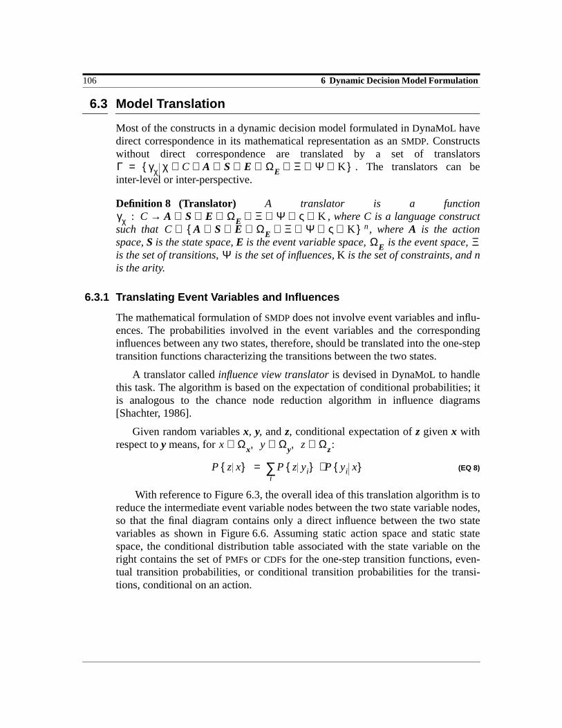
106 6 Dynamic Decision Model Formulation
6.3 Model Translation
Most of the constructs in a dynamic decision model formulated inDynaMoL havedirect correspondence in its mathematical representation as anSMDP. Constructswithout direct correspondence are translated by a set of translators
. The translators can beinter-level or inter-perspective.
Definition 8 (Translator) A translator is a function, where C is a language construct
such that , whereA is the actionspace,S is the state space,E is the event variable space, is the event space,is the set of transitions, is the set of influences,K is the set of constraints, and nis the arity.
6.3.1 Translating Event Variables and Influences
The mathematical formulation ofSMDP does not involve event variables and influ-ences. The probabilities involved in the event variables and the correspondinginfluences between any two states, therefore, should be translated into the one-steptransition functions characterizing the transitions between the two states.
A translator calledinfluence view translatoris devised inDynaMoL to handlethis task. The algorithm is based on the expectation of conditional probabilities; itis analogous to the chance node reduction algorithm in influence diagrams[Shachter, 1986].
Given random variablesx, y, andz, conditional expectation ofz givenx withrespect toy means, for :
(EQ 8)
With reference to Figure 6.3, the overall idea of this translation algorithm is toreduce the intermediate event variable nodes between the two state variable nodes,so that the final diagram contains only a direct influence between the two statevariables as shown in Figure 6.6. Assuming static action space and static statespace, the conditional distribution table associated with the state variable on theright contains the set ofPMFs orCDFs for the one-step transition functions, even-tual transition probabilities, or conditional transition probabilities for the transi-tions, conditional on an action.
Γ γχ χ C A S E ΩE Ξ Ψ K∪ ∪ ∪ ∪ ∪ ∪⊆∈ =
γχ : C A S E ΩE Ξ Ψ ς K∪ ∪ ∪ ∪ ∪ ∪ ∪→C A S E ΩE Ξ Ψ ς K∪ ∪ ∪ ∪ ∪ ∪ ∪ n⊆
ΩE ΞΨ
x Ωx∈ y Ωy∈ z Ωz∈, ,
P z x P z yi P yi x ⋅i
∑=

6.3 Model Translation 107
Figure 6.6 Final influence view after reduction by the influence translator.
In essence, the influence view translator iteratively identifies an event variablenode to be reduced, updates the conditional distributions of other event variablesaffected by it, and removes it. The main algorithm is as follows:
INFLUENCE-VIEW-TRANSLATOR (ID)
◊ ID is a sequence of event-variable-nodesx ← FIND-REMOVABLE-EVENT-VARIABLE (ID)while x
do ID ← ABSORB-EVENT-VARIABLE (ID, x)x ← FIND-REMOVABLE-EVENT-VARIABLE (ID)
return ID
An event variable node is removable only if it has a single probabilistic succes-sor. A simple heuristic is employed to remove event variable nodes with smallerconditional distribution dimensions first. This heuristic helps keep the size of theconditional distribution tables to be updated as small as possible.
FIND-REMOVABLE -EVENT-VARIABLE (ID)
◊ ID is a sequence of event-variable-nodesE-list ← ∅for each x∈ ID
unless x = state-variable or x = next-state-variable do if length[successors[x]] = 1
then E-list ← E-list ∪ x◊ Sort elements of E-list according to the increasing number of predecessorsnodes and the increasing size of (lone) successor.return first[E-list]
To remove an event variable nodex, its lone successory must inherit its prede-cessors, and the conditional distribution ofy must be updated accordingly. Simi-larly, x will no longer be a successor to all its predecessors.
ABSORB-EVENT-VARIABLE (ID, x)
◊ ID is a sequence of event-variable-nodes, x is an event-variable-node.Dx ← distribution-table[x]y ← first[successors[x]] ◊ Assume x has only one successor.
STATE-N STATE
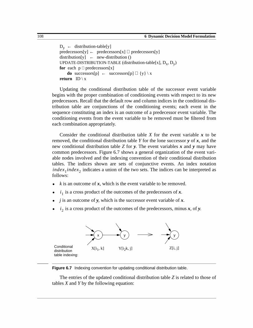
108 6 Dynamic Decision Model Formulation
Dy ← distribution-table[y]predecessors[y]← predecessors[x]∪ predecessors[y]distribution[y] ← new-distribution ()UPDATE-DISTRIBUTION-TABLE (distribution-table[x], Dx, Dy)for each p∈ predecessors[x]
do successors[p] ← successors[p]∪ y \ xreturn ID \ x
Updating the conditional distribution table of the successor event variablebegins with the proper combination of conditioning events with respect to its newpredecessors. Recall that the default row and column indices in the conditional dis-tribution table are conjunctions of the conditioning events; each event in thesequence constituting an index is an outcome of a predecessor event variable. Theconditioning events from the event variable to be removed must be filtered fromeach combination appropriately.
Consider the conditional distribution tableX for the event variablex to beremoved, the conditional distribution tableY for the lone successory of x, and thenew conditional distribution tableZ for y. The event variablesx andy may havecommon predecessors. Figure 6.7 shows a general organization of the event vari-able nodes involved and the indexing convention of their conditional distributiontables. The indices shown are sets of conjunctive events. An index notation
indicates a union of the two sets. The indices can be interpreted asfollows:
• k is an outcome ofx, which is the event variable to be removed.
• is a cross product of the outcomes of the predecessors ofx.
• j is an outcome ofy, which is the successor event variable ofx.
• is a cross product of the outcomes of the predecessors, minusx, of y.
Figure 6.7 Indexing convention for updating conditional distribution table.
The entries of the updated conditional distribution tableZ is related to those oftablesX andY by the following equation:
index1index2
i1
i2
x y y
Conditional X[i 1, k] Y[i 2k, j] Z[i, j]distributiontable indexing:
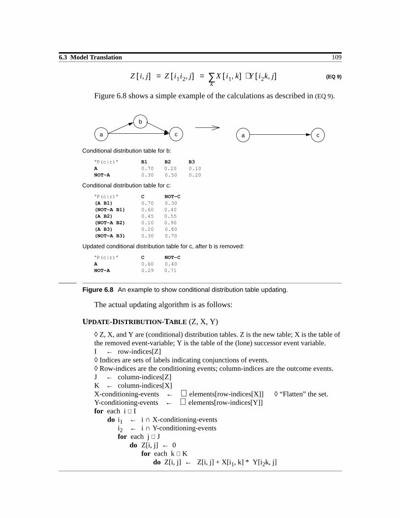
6.3 Model Translation 109
(EQ 9)
Figure 6.8 shows a simple example of the calculations as described in(EQ 9).
Conditional distribution table for b:
“P(c|r)” B1 B2 B3A 0.70 0.20 0.10NOT-A 0.30 0.50 0.20
Conditional distribution table for c:
“P(c|r)” C NOT-C(A B1) 0.70 0.30(NOT-A B1) 0.60 0.40(A B2) 0.45 0.55(NOT-A B2) 0.10 0.90(A B3) 0.20 0.80(NOT-A B3) 0.30 0.70
Updated conditional distribution table for c, after b is removed:
“P(c|r)” C NOT-CA 0.60 0.40NOT-A 0.29 0.71
Figure 6.8 An example to show conditional distribution table updating.
The actual updating algorithm is as follows:
UPDATE-DISTRIBUTION -TABLE (Z, X, Y)
◊ Z, X, and Y are (conditional) distribution tables. Z is the new table; X is the table ofthe removed event-variable; Y is the table of the (lone) successor event variable.I ← row-indices[Z]◊ Indices are sets of labels indicating conjunctions of events.◊ Row-indices are the conditioning events; column-indices are the outcome events.J ← column-indices[Z]K ← column-indices[X]X-conditioning-events ← ∪ elements[row-indices[X]] ◊ “Flatten” the set.Y-conditioning-events ← ∪ elements[row-indices[Y]]for each i∈ I
do i1 ← i ∩ X-conditioning-eventsi2 ← i ∩ Y-conditioning-eventsfor each j∈ J
do Z[i, j] ← 0for each k∈ K
do Z[i, j] ← Z[i, j] + X[i 1, k] * Y[i 2k, j]
Z i j,[ ] Z i1i2 j,[ ] X i1 k,[ ] Y i2k j,[ ]⋅k∑= =
ca
b
ca

110 6 Dynamic Decision Model Formulation
Assuming that each event variable involved has m outcomes andn predeces-sors on average, the number of conditional distribution table entries to be updatedis .
For the influence view of the case study as shown in Figure 6.3, the state vari-able and the next-state variable have 18 and 19 outcomes each, and the other eventvariables have an average number of 3 outcomes. Applying the influence viewtranslator algorithm as described above, the most common table updating involvesthe next-state variable, with about 3 other event variables and the state variable asits predecessors. To reduce an event variable from an influence view, the numberof table entries that need to be calculated is of the order of 8700; the addition ofone more predecessor would make it to the order of 26,000! This is the main moti-vation for introducing the partialOR-gate, which drastically cuts down the sizes ofthe intermediate conditional distribution tables in practice.
6.3.2 Translating Declaratory Constraints
Most declaratory constraints have direct correspondence in theSMDP representa-tion. Each state variable, for instance, corresponds to the state-space at a particulartime or decision stage in theSMDP.
The only explicit translator currently defined inDynaMoL is a translator for thepartialOR-gate constraint. Recall that this constraint can be expressed in terms ofan implication statement. The antecedent contains the constraining events in dis-junctive form; the consequent represents the target definition for the constrainingevents. The corresponding translator is encoded as a special version of the updatedistribution table algorithm described in Section 6.3.1. This new algorithm is usedwhen the event variablex to be removed, or its lone successory, or both containconditional distribution tables with the partialOR-gate constraints. In other words,some of the indices of these tables are sequences or sets of labels representing dis-junctions of events. Recall also that currently only one partialOR-gate can beimposed on each event variable.
Let be the table entries forx, be the table entries fory, and be the table entries for the updated table ofy. A constraining row index is a
row index in disjunctive form, representing all of the constraining events in thepartial OR-gate. A constrainingpartial row index is a row index in disjunctiveform, representingsome of the constraining events in the partialOR-gate. Forinstance,[DIE DIE-GIB DIE-CHM DIE-TE] is a constraining row index,[DIE-GIB DIE-TE]
is a constraining partial row index for the partialOR-gate defined with respect toFigure 6.4. Similar, a constrained column index represents the consequent event ina partialOR-gate. For instance,DEAD-A is a constrained column index for the aboveexample.
The translator needs to consider three cases:
O mn 1+ )(
X i1 k,[ ] Y i2k j,[ ]Z i j,[ ]
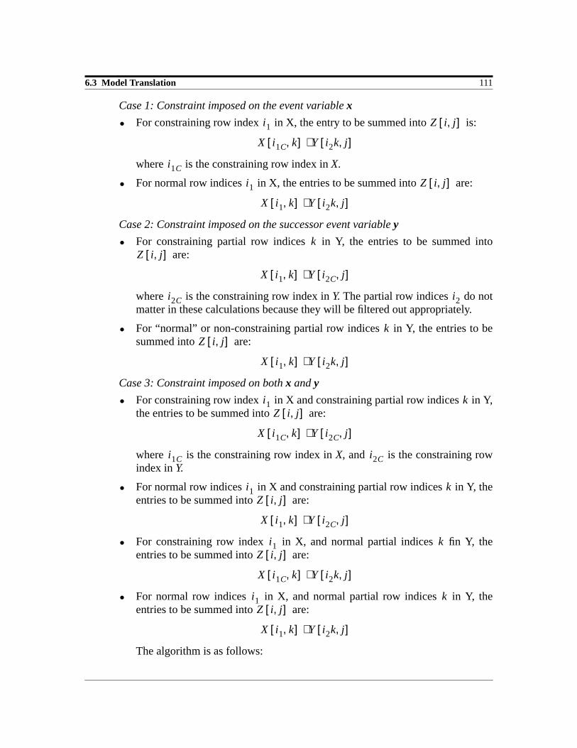
6.3 Model Translation 111
Case 1: Constraint imposed on the event variablex
• For constraining row index in X, the entry to be summed into is:
where is the constraining row index inX.
• For normal row indices in X, the entries to be summed into are:
Case 2: Constraint imposed on the successor event variabley
• For constraining partial row indices in Y, the entries to be summed into are:
where is the constraining row index inY. The partial row indices do notmatter in these calculations because they will be filtered out appropriately.
• For “normal” or non-constraining partial row indices in Y, the entries to besummed into are:
Case 3: Constraint imposed on bothx andy
• For constraining row index in X and constraining partial row indices in Y,the entries to be summed into are:
where is the constraining row index inX, and is the constraining rowindex inY.
• For normal row indices in X and constraining partial row indices in Y, theentries to be summed into are:
• For constraining row index in X, and normal partial indices fin Y, theentries to be summed into are:
• For normal row indices in X, and normal partial row indices in Y, theentries to be summed into are:
The algorithm is as follows:
i1 Z i j,[ ]
X i1C k,[ ] Y i2k j,[ ]⋅
i1C
i1 Z i j,[ ]
X i1 k,[ ] Y i2k j,[ ]⋅
kZ i j,[ ]
X i1 k,[ ] Y i2C j,[ ]⋅
i2C i2
kZ i j,[ ]
X i1 k,[ ] Y i2k j,[ ]⋅
i1 kZ i j,[ ]
X i1C k,[ ] Y i2C j,[ ]⋅
i1C i2C
i1 kZ i j,[ ]
X i1 k,[ ] Y i2C j,[ ]⋅
i1 kZ i j,[ ]
X i1C k,[ ] Y i2k j,[ ]⋅
i1 kZ i j,[ ]
X i1 k,[ ] Y i2k j,[ ]⋅

112 6 Dynamic Decision Model Formulation
UPDATE-DISTRIBUTION -TABLE -WITH -CONSTRAINTS (Z X, Y)
◊ Z, X, and Y are (conditional) distribution tables. Z is the new table; X is the tableof the removed event-variable; Y is the table of its (lone) successor.I ← row-indices[Z]◊ Indices are sequences or sets of labels indicating conjunctions or disjunctions ofevents.◊ Row-indices are the conditioning events; column-indices are the outcome events.J ← column-indices[Z]K ← column-indices[X]i1C ← constraining-row-index[X]i2C ← constraining-row-index[Y]X-conditioning-events ← ∪ elements[row-indices[X]] ◊ “Flatten” the set.Y-conditioning-events ← ∪ elements[row-indices[Y]]for each i∈ I
do i1 ← i ∩ X-conditioning-eventsi2 ← i ∩ Y-conditioning-eventsfor each j∈ J
do Z[ i, j ] ← 0for each k∈ K
do if constraining? (i1)then if constraining? (k)
then Z[i, j] ← Z[i, j] + X[i 1C, k] * Y[i 2C, j]else Z[i, j] ← Z[i, j] + X[i1C, k] * Y[i 2k, j]
else if constraining? (k)then Z[i, j] ← Z[i, j] + X[i 1, k] * Y[i 2C, j]else Z[i, j] ← Z[i, j] + X[i1, k] * Y[i 2k, j]
The number of table entries to be updated is of about the same order as before: wherem is the average number of outcomes andn is the average
number of predecessors of an event variable. The smaller dimensions of the condi-tional distribution tables rendered by the partialOR-gate, however, makes a big dif-ference in computational costs in practice.
Explicit translations for other declaratory constraints such as numeric restric-tion on the events are not currently handled inDynaMoL.
6.3.3 Translating Strategic Constraints
The only strategic constraints supported by the current version ofDynaMoL ontol-ogy are on the applicability of the actions in the states. Given the state space, thestates in which an action are not applicable are specified as absorbing states. Noexplicit translators are devised for such strategic constraints.
O m 1−( ) n 1+( )

113
7 Dynamic DecisionModel Solutionand Analysis
Once the dynamic decision model is formulated and translated into anSMDP, themodel can be solved by any solution methods forSMDPs. Analysis can be carriedout on both the model and its correspondingSMDP. This chapter discusses someapplicable solution methods and the types of relevant analysis.
7.1 Solution Methods
A variety of solution methods are available forSMDPs. We examine in detail thetwo solution methods implemented in the current version ofDYNAMO : value-itera-tion and fundamental matrix solution. We also briefly mention other availablemethods. Admitting various solution methods is a major feature of theDynaMoLarchitecture. Based on the characteristics of the dynamic decision problem con-cerned, we can choose the most efficient solution method available.
7.1.1 Value Iteration
A dynamic decision problem can be expressed as the dynamic programming equa-tion, or Bellman optimality equation, of anSMDP. For a decision horizon ofnstages, with a discount factor , the optimal value achievable in any state
, , given an initial value and current time , is [Howard, 1971]:0 β≤ 1<
i S∈ Vi* Vi 0( ) t T∈

114 7 Dynamic Decision Model Solution and Analysis
(EQ 10)
where
is the one-step transition function from statei to j, conditional on actiona, fordurationm after entering a statei at timet; and
is the transition value function with yield rate and bonus for transi-tion such that
denotes the objective value achievable in each state over durationm, condi-tional on action .
The first addend in(EQ 10) indicates the expected value achievable if the nexttransition out of statei occurs after time durationn, and the second addend indi-cates the expected value achievable if the next transition occurs before time dura-tion n. In the specialized case of anMDP, (EQ 10) specializes into(EQ 2’) asdescribed in Section 2.3 and reproduced below:
(EQ 11)
The value iteration solution method is to solve the optimality equation shownin (EQ 10) or (EQ 11). The solution to such an equation is an optimal policy
where and , that maximizes , the optimalexpected value or reward for an initial state over durationN, at time . Recallthat is the remaining duration for the decision horizon.
Vi* n β t, ,( )
n 0 i j S∈ a A t T∈,∈, , ,≥
+ qija( ) m t,( ) βl yi
a( ) l( ) βmbija( ) βm+ Vj
* n m− β t m+, ,( )+l 0=
m 1−
∑ ;m 1=
n
∑j
∑
maxa qija( ) m t,( ) βl yi
a( ) l( ) βnVi 0( )+l 0=
n 1−
∑m n 1+=
∞
∑j
∑=
qija( ) m t,( ) Pij
a( ) t( ) hija( ) m t,( )⋅=
vija( ) m( ) yi
a( ) l( )l 0=m 1−∑[ ] bij
a( )+=
yia( ) .( ) bij
a( )
ξ a i j t, , ,( )
via( ) m( ) qij
a( ) .( ) vija( ) m( )
j∑=
i S∈a A∈
Vi* n β t, ,( ) maxa vi
a( ) 1( ) β Pijk( ) t( ) Vj
* n 1− β t, 1+,( ) ;⋅j
∑+=
n 0 i j S∈ a A t T∈,∈, , ,≥
π* µ0* µ1
* µ2* µ3
* … , , , ,=
µt* : S A→ t T∈ Vinit
* N β 0, ,( )t 0=
n N t−=

7.1 Solution Methods 115
For a decision horizon of durationN, the complexity of the value iterationalgorithm forSMDP is , since in each decision stage, we gener-ally need to consider all time points such that . The complexity ofthe corresponding algorithm forMDP is ; in this case there is aone-to-one correspondence between the durationn and the current timet:
.
As mentioned, all the default solution methods in existing dynamic decisionmodeling techniques are based on value iteration. While probabilistic inferencetechniques can also be employed for solving dynamic influence diagrams[Shachter and Peot, 1992], the graph reduction algorithm [Tatman andShachter, 1990] corresponds directly to Markov value iteration. The graph roll-back algorithm for stochastic trees [Hazen, 1992] also corresponds directly tovalue iteration. Cohort analysis and Monte Carlo simulation in Markov cycle trees,however, are based on conditional expectation in a forward manner; the complex-ity of these algorithms is since they do not make use of thememoized optimal substructures inherent in dynamic programming techniques.
Currently, four different versions of the value iteration method are imple-mented inDYNAMO: semi-Markov value iteration as described in(EQ 10) for solv-ing discrimination problems and optimization problems, and Markov valueiteration as described in(EQ 11) for discrimination problems and optimization prob-lems. The discrimination versions simply ignore the maximization step involvedand compute the expected value with respect to each controlled action indi-vidually.
The first clinical question for the case study is posed as a discrimination prob-lem; the numeric parameters are assessed in accordance with anMDP, i.e, withconstant holding times. The solution produced by the solver is a set of two poli-cies, corresponding to the four strategies considered; each policy includes theexpected value achievable for all possible starting states and all possible decisionstages. We assume that the patient has a probability of 0.25 to be in atrial fibrilla-tion, has no history of thromboembolism, and is not on warfarin at the beginningof the decision horizon. The results indicate that the strategy that administers onlywarfarin initially is the preferred strategy over a long-term decision horizon of 50years or 600 months.
The second clinical question for the case study is posed as an optimizationproblem; the numerical parameters are assessed in accordance with anSMDP. Thesolution produced by the solver is an optimal policy for all possible starting statesand all possible decision stages. We adopt the same assumptions about the condi-tion of the patient as mentioned. For a short-term decision horizon of 5 years or 60months, the results indicate that the strategy that administers only warfarin initiallyis the preferred strategy up to 8 months. After 8 months, if the patient remains inthe same condition, the strategy that does not administer any drug initially is pre-ferred.
O N2 A S 2⋅ ⋅( )t' t t' t n+≤ ≤
O N A S 2⋅ ⋅( )
n N t−=
O S A S⋅( ) N⋅( )
a A∈

116 7 Dynamic Decision Model Solution and Analysis
7.1.2 Fundamental Matrix Solution
If the durationN for the decision horizon is large, the problem can be formulatedwith an infinite decision horizon. For infinite horizon problems with homogeneousor time-independent one-step transition functions,(EQ 10) simplifies to:
(EQ 12)
The corresponding equation for the Markov case is:
(EQ 13)
7.1.3 Other Methods
Although not currently implemented inDYNAMO, DynaMoL admits many othersolutions methods. Solution methods reported in theMDPs andSMDPs literaturesuch aspolicy iteration [Howard, 1960],adaptive aggregation [Bertsekas, 1987],or linear programming are directly applicable if certain assumptions or conditionsare met. These conditions include stationary policies, constant discount factors,homogeneous transition functions,etc. Some of these methods are summarized inAppendix B.
As mentioned in Section 2.5, recent research in decision-theoretic planning hasalso led to new solution methods forMDPs [Dean et al., 1993a] [Deanet al., 1993b] [Deardon and Boutilier, 1994] [Drummond and Bresina, 1990][Kushmerick et al., 1994]. These methods address the trade-off between solutionoptimality and computation cost in complex and time-critical decision domains.
Besides the solution methods forMDPs andSMDPs, other solution methods thattake advantage of the high levelDynaMoL ontology can also be employed. Weexplore how these methods can be devised in Chapter 8.
In summary, by separating the modeling task supported by the decision gram-mar and graphical presentation, and the solution task supported by the mathemati-cal representation, a large collection of solution methods can be employed inDynaMoL. Moreover, employing a new solution method does not involve anychange to the high level modeling language itself; all solution methods referenceonly the mathematical representation of a model. Similarly, extending or adaptingthe decision grammar and graphical presentation do not affect the solution meth-
Vi* β( ) maxa qij
a( ) m( ) βl yia( ) l( ) βmbij
a( ) βmVj* β( )+ +
l 0=
m 1−
∑m 1=
∞
∑j
∑ ;=
i j S∈, a A∈;
Vi* β( ) maxa vi
a( ) 1( ) β Pija( ) Vj
* β( )⋅j
∑+ ;=
i j S∈ a A∈, ,

7.2 Sensitivity Analyses 117
ods already applicable; these may, however, admit other solution methods thatmake use of the additional constructs.
7.2 Sensitivity Analyses
To assess the accuracy, conciseness, and clarity of a dynamic decision model for-mulated inDynaMoL, sensitivity analyses are often performed. Such analyses canlead to revision of the structural and numerical parameters of the model. Althoughnot currently implemented, various model quality metrics described in Section3.3.3 can be used in theDynaMoL framework. Adequate support for sensitivityanalyses is essential for a practical dynamic decision modeling language. The cur-rent version ofDynaMoL provides basic support for such analyses. Additional fea-tures can be incorporated as we extend the language and the implementation.
The graphical presentation convention and precise mathematical properties oftheDynaMoL ontology facilitate analysis of the structural and numerical parame-ters of the model. Structural parametric analysis is done by removing or addingsome event variables. The influence view supports such local structural changes.In addition to determining and analyzing the information involved in the changes,the revised models will also be translated into and solved asSMDPs to examine thechanges in solution results. On the other hand, the transition view makes it easierto detect improperly specified parameters. For instance, there should not be a tran-sition from a state where warfarin is ineligible to one where warfarin is adminis-tered. Currently there is no support for reverse translation, hence changes made tothe underlyingSMDP cannot be reflected in the high level components of thedynamic decision model.
Numerical parametric analysis is done by simply changing some of the transi-tion and value functions in theSMDP and invoking the solution method. Usually notranslation of the model is necessary.
In the case study, we conducted only numerical parametric analysis. Theresults are described in detail in Appendix C. For the long-term discriminationproblem, the results indicate that the strategy of administering only warfarin butnot Quinidine to the patient is the dominant strategy for all reasonable ranges ofnumerical parameters involved. For the short-term optimization problem, theresults demonstrate that over the decision horizon, the preferred strategy shifts in areasonable manner from initially administering warfarin to no drug, depending onthe desirable and the undesirable effects of warfarin.
The mathematical representation ofSMDP also facilitates analysis of the natureof a solution to a dynamic decision model. Given a specific solution method, muchinsights can be gained about the solution by examining the nature of the statespace, action space, and other decision parameters. For instance, if absorbing

118 7 Dynamic Decision Model Solution and Analysis
states are present in a well-formedSMDP, convergence is guaranteed in value itera-tion.

119
8 LanguageEnhancement andPracticalDevelopment
Besides addressing the trade-off between model transparency and solution effi-ciency,DynaMoL is a flexible framework designed to be extensible, adaptable, andpractical. In Chapter 7, we have described how the current version ofDynaMoLsupports dynamic decision modeling with multiple perspective reasoning; all thecapabilities mentioned are implemented in theDYNAMO system. In this chapter,we examine how the language features and system capabilities can be extended,adapted, and developed for general practical applications. The discussion high-lights the desirable, the feasible, and the inherently difficult aspects of languageenhancement and practical development of theDynaMoL framework.
8.1 Supporting Language Extension and Adaptation
Language enhancement includes extending and adapting the basic decision ontol-ogy in DynaMoL. Extension improves language expressiveness; it often involvesaddition or generalization of the dynamic decision grammar constructs, the graphi-cal presentation perspectives, and theSMDP definitions. Adaptation improves lan-guage transparency or clarity; it often involves addition or reorganization of thegrammar constructs and presentation perspectives, while the underlyingSMDP def-initions remain unchanged. This may in turn support solution methods that canmake use of the rearranged representation.
DynaMoL supports incremental extension and adaptation. In general, languageextension and adaptation are achieved by introducing a set of new grammar con-structs or presentation formats or both, and devising a set of translators for them.This section sketches the approaches to addressing some of these issues.

120 8 Language Enhancement and Practical Development
8.1.1 Static vs. Dynamic Spaces
The current version ofDynaMoL assumes static state spaceS and static actionspaceA. In a static state space, the same states are valid throughout the decisionhorizon. In a static action space, the same set of actions are applicable in each stateover all time points or decision stages. We can model dynamic state space or actionspace by providing “dummy” states and “no-op” actions. Such extraneous entities,however, may compromise model clarity and solution efficiency in practice.
The DynaMoL decision grammar can be easily extended to incorporatedynamic state space and dynamic action space. New productions for the corre-sponding constructs can be written to incorporate the valid time or duration foreach state and action. The graphical presentation convention remains mostlyunchanged; only the valid entities are displayed for particular time points or deci-sions stages.
These new constructs directly correspond to the general classes of semi-Markov decision processes with dynamic state space and dynamic action space asdefined in Section 3.3.1.
8.1.2 Automatic State Augmentation
State augmentation is a basic technique for incorporating extra information in theSMDP framework. Most of the declaratory and strategic constraints, for instance,can be represented as state attribute variables. In other words, the constraints areincorporated as additional dimensions of the state space. It is the user’s responsi-bility to identify the relevant constraints and incorporate them into the state spacedirectly; the associated numerical parameters are then assessed accordingly.
From a modeling point of view, constraints such as numeric restriction onsome events affect only part of the original state space. For example, if one of theoriginal state attribute variables indicates whether the patient has a stroke before,the constraint on the number of stroke only affects those states that involve astroke. Therefore, it is more convenient to specify such constraints and their asso-ciated parameters separately, and have a set of translators to automatically incorpo-rate the information. This involves working with an abstract state space, whichwill eventually be translated into the full state space for solution and analysis. Thisapproach would allow us to incrementally and separately impose various con-straints, without directly dealing with the resulting large and complex state space.
Automatic state augmentation can be achieved inDynaMoL by adding a set ofgrammar constructs for specifying the constraints, and a set of translators for trans-lating them to form a state space of larger dimension. Similarly, additional con-structs and translators are needed for the associated parameters.
This idea of modeling in an abstract state space for transparency is directlyopposite to the idea of execution or solution in an abstract state space for effi-

8.1 Supporting Language Extension and Adaptation 121
ciency. The latter idea is adopted asaggregation methods in control theory[Bertsekas, 1987], and ashierarchicalor abstraction planning methods in non-lin-ear AI planning [Knoblock, 1991] [Korf, 1987] [Stefik, 1981] [Sacerdoti, 1974][Sacerdoti, 1975] [Tate, 1977] and decision-theoretic planning [Deardon andBoutilier, 1994].
Sometimes it is desirable to freely access the multiple levels of abstraction in adynamic decision model for both modeling and solution. Although we do notknow if it is feasible in general, this may be achieved by devising a set of two-waytranslators inDynaMoL. This issue is left for future exploration.
8.1.3 Limited Memory
As compared to a Markov process, a semi-Markov process supports a seconddimension of uncertainty: time spent in a state before transition. A semi-Markovprocess is only “semi-” Markov because there is a limited memory of the timeduration since entry into any particular state. In some cases, memory about previ-ous states or actions is important in a dynamic decision problem. For example, if apatient had a heart attack before, he would be more susceptible to a second heartattack during surgery. Such limited memory can be incorporated into a semi-Markov or Markov process by state augmentation, either directly or automaticallyas described above.
Repeated applications of state augmentation usually lead to an explosion of thestate space size. To avoid such explosion, we can relegate the solution methods tokeep track of limited memory. Only forward induction based solution methods,however, are applicable. In this approach, a new counter or binding calledmemoryor history can be introduced to keep track of the relevant states that a process hasvisited. Calculations of the expected value with respect to the model parametersare now conditional on the history accumulated so far. In other words, the parame-ters are specified in terms of conditional statements. For instance, if a particularpatient has a heart attack before, then the probability of his having another heartattack in the next year is 0.3, otherwise, it is 0.15.
A set of history constructs can be introduced inDynaMoL to keep track of thelimited memory, and a set of translators for the conditional parametric specifica-tion are needed. The solution methods can then operate on both theSMDP and thehistory constructs.
8.1.4 Numeric and Ordering Constraints
Numeric and ordering constraints are closely related to the limited memory capa-bilities. There are several types of such constraints: Event or state numeric con-straints specify that a certain number of events or states will lead to a specificconsequence, e.g., a patient is assumed dead if he has had three strokes. Action

122 8 Language Enhancement and Practical Development
numeric constraints restrict the number of times an action may be applied. Actionordering constraints specify that an action must always or never follow anotheraction.
As in limited memory, there are two methods to incorporate such constraintsinto a dynamic decision model. The first method is to augment the state space tokeep track of the number or the order of the decision factors. For instance, a trans-lator for the numeric restriction constraint can be developed in the following man-ner: Add an additional state attribute variable for the constraint,e.g.,number ofstroke. For each event or state whose number is to be restricted, establish an influ-ence from the corresponding event variable or state variable to the new stateattribute variable. Finally, establish an influence from the new state attribute vari-able to every state in the next-state variable that is affected by the numeric restric-tion whose number is to be restricted.
The second method is to introduce a set of counters and let the solution meth-ods worry about keeping track of the constraints. Again new constructs and trans-lators are needed to incorporate the constraints. To facilitate proper translations, anexternal knowledge based system can be employed to choose the right translatorsby examining the nature of the constraints and solution methods.
8.1.5 Canonical Models of Combination
In the previous chapter, we have demonstrated how the partial-OR constraint onevent combination can be incorporated inDynaMoL. Other general or domain spe-cific constraints or canonical models can be introduced in a similar manner.
8.1.6 Presentation Convention
So far we have described two graphical presentation perspectives inDynaMoL: thetransition view and the influence view. Each perspective illuminates the dynamicdecision problem in a different way, and facilitates modeling at a different level ofgranularity. Other useful presentation perspectives can be incorporated by intro-ducing new presentation conventions and translators.
For instance, asymmetric probabilistic relations are not structurally shown inthe influence view; a tree-like perspective is more convenient for illuminating suchrelations. Consider the piece of knowledge: “A patient may have a chance ofthromboembolization, the outcomes may be a stroke, a transient ischemic attack,or no thromboembolization. If he has a stroke, it may be permanent or transient,and there is a chance that he will die from the stroke.” Figure 8.1 shows a partialinfluence view that represents the above knowledge. The asymmetry involved isembedded in the conditional distribution table. If we can expand the event vari-ables and the probabilistic relations involved into a tree, as shown in Figure 8.2,
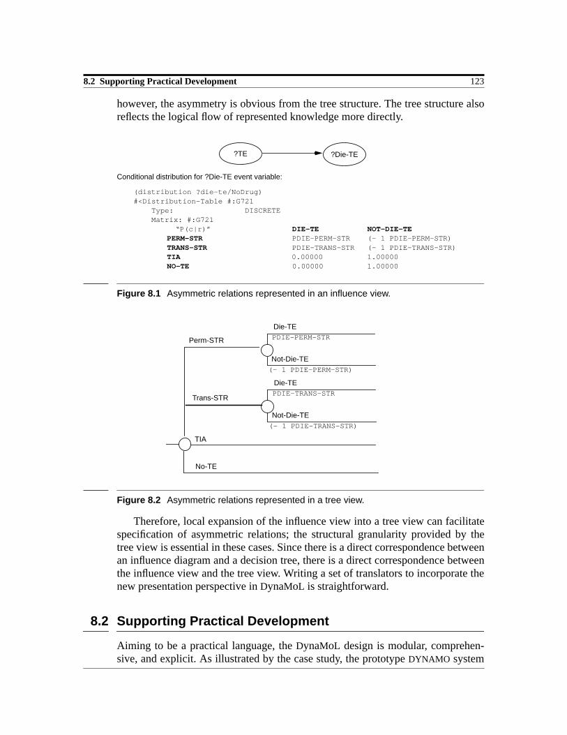
8.2 Supporting Practical Development 123
however, the asymmetry is obvious from the tree structure. The tree structure alsoreflects the logical flow of represented knowledge more directly.
Conditional distribution for ?Die-TE event variable:
(distribution ?die-te/NoDrug)#<Distribution-Table #:G721 Type: DISCRETE Matrix: #:G721
“P(c|r)” DIE-TE NOT-DIE-TEPERM-STR PDIE-PERM-STR (- 1 PDIE-PERM-STR)TRANS-STR PDIE-TRANS-STR (- 1 PDIE-TRANS-STR)TIA 0.00000 1.00000NO-TE 0.00000 1.00000
Figure 8.1 Asymmetric relations represented in an influence view.
Figure 8.2 Asymmetric relations represented in a tree view.
Therefore, local expansion of the influence view into a tree view can facilitatespecification of asymmetric relations; the structural granularity provided by thetree view is essential in these cases. Since there is a direct correspondence betweenan influence diagram and a decision tree, there is a direct correspondence betweenthe influence view and the tree view. Writing a set of translators to incorporate thenew presentation perspective inDynaMoL is straightforward.
8.2 Supporting Practical Development
Aiming to be a practical language, theDynaMoL design is modular, comprehen-sive, and explicit. As illustrated by the case study, the prototypeDYNAMO system
?TE ?Die-TE
TIA
No-TE
Perm-STR
Trans-STR
Die-TE
Not-Die-TE
PDIE-PERM-STR
(- 1 PDIE-PERM-STR)
Die-TE
Not-Die-TE
PDIE-TRANS-STR
(- 1 PDIE-TRANS-STR)

124 8 Language Enhancement and Practical Development
can handle a class of actual dynamic decision problems in medicine. On the theo-retical side, incorporating the possible language enhancement discussed abovewould allow the system to model and solve a larger class of problems. On the prac-tical side, we propose a set of support tools that would make the system more con-venient to use. This section summarizes the desirable support tools and sketcheshow these tools can be incorporated into the currentDYNAMO architecture.
8.2.1 Editing and Specification Support
Structural parameters such as actions, states, and event variables can be specifiedin DYNAMO through either the graphical interface or Common Lisp code. On theother hand, numerical parameters, which mostly involve the conditional distribu-tions of event variables, can only be specified through a simple table editor. Sincemany of the table entries are repetitive or related by probabilistic constraints, moresophisticated table editing support can be very helpful. Some examples of suchsupport include spreadsheet editors and equation editors. These tools can be addeddirectly to theDYNAMO system architecture.
8.2.2 Statistical Analysis
Numerical sensitivity analysis on the dynamic decision model is conductedthrough standard statistical techniques such as one-way or two-way regression.Such statistical capabilities can be added toDYNAMO. Alternately, external func-tion interfaces or hooks can be incorporated to access a readily available statisticalpackage.DYNAMO has a separately modifiable module for recording and printing asolution in different ways. The solution data can be easily piped to an external sta-tistical module or package.
8.2.3 Data Visualization
Throughout this work, we have emphasized that information visualization is essen-tial for facilitating dynamic decision modeling. Such visualization not only helpsin debugging the model parameters, but also provides useful insights to the under-lying natural phenomena. The presentation perspectives mentioned earlier illumi-nate both structural and numerical information in a model. Other presentationformats such as two- or three-dimensional Cartesian plots are helpful in visualiz-ing the numerical data in different ways. The data plotters can be incorporated intotheDYNAMO graphical interface in a straightforward manner.

125
9 Conclusion
We conclude by reflecting on the lessons learned in this research. First, we summa-rize the achievements and limitations of this work. Then, we compare ourapproaches and results with some related work. Finally, we point out some direc-tions for future research.
9.1 Summary
We set out to compare and contrast existing methodologies for addressing a sub-class of dynamic decision problems. We identified semi-Markov decision pro-cesses (SMDPs) as a common basis among the current techniques. Building on thecommon basis by integrating different features of these techniques, we proposed anew general methodology for dynamic decision making under uncertainty. Weintroduced multiple perspective reasoning and incremental language extension asthe central ideas of this new methodology.
To informally evaluate the feasibility and effectiveness of the new ideas, weimplemented them in a prototype system; we also conducted a detailed case studyto formulate and solve two dynamic decision problems in medicine. The prototypesystem produced adequate solutions for the case study, and showed desirable sup-port for general dynamic decision modeling. This exercise demonstrated the prac-tical promise of the proposed framework.
9.1.1 The Analysis
The analysis of three major approaches to dynamic decision making under uncer-tainty highlighted their similarities and differences, as well as their strengths andweaknesses.

126 9 Conclusion
SMDPs are formal mathematical models with rigorous definitions but limitedflexibility. While they can express a general class of stochastic models, they pro-vide very little organizational support for the knowledge involved. The preciselyencoded knowledge is difficult to specify and access since many assumptions arebuilt in. TheSMDP approach, therefore, is difficult to apply in practice.
Dynamic decision modeling provides graphical support for specifying andaccessing the information involved. Different types of information, however, aremore clearly depicted in different dynamic decision models. Moreover, the graphi-cal model structures usually restrict the solution methods applicable.
Decision-theoretic planning techniques establish guidelines and methods toefficiently solve dynamic decision problems in large and complex domains. UnlikeSMDPs and dynamic decision models, these techniques do not assume a completelyenumerable state space or decision environment. There is no uniform planningframework. The underlying theoretical basis, however, is usually a subclass ofSMDPs, the Markov decision processes (MDPs). Most of the insights and results arestill experimental, and may not be applicable in general asSMDPs and dynamicdecision models.
9.1.2 The Unifying View
Based on a uniform task definition for dynamic decision making under uncertainty,we explicated the representational and inferential support involved. We alsoexplained how the other techniques can be formulated in terms of theSMDPsframework.
We propose thatSMDPs be regarded the same role in dynamic decision makingunder uncertainty as first-order predicate calculus(FOPC) in deterministic knowl-edge representation. Recently, [Dean, 1994] has independently come up with thesame idea forMDPs to be regarded as the basis for decision-theoretic planning. Wehave further illustrated the motivation for our proposal by devising a new method-ology based on the idea.
9.1.3 The General Methodology
The new methodology adopted inDynaMoL aims to balance the trade-off betweenmodel transparency and solution efficiency. It supports information visualizationand access from different angles, facilitating different aspects of problem solving.It also promotes the use of translators to enhance language ontology and differenti-ate the modeling task from the solution or execution task. We demonstrated how towrite such translators, specifically with the development of the partial-OR gateconstraint on event combination.
Model specification inDynaMoL is in terms of a higher level language thanthat in existing dynamic decision modeling frameworks. In frameworks such as

9.1 Summary 127
dynamic influence diagrams or Markov cycle trees, the model parameters need tobe explicitly specified in detail. In particular, the declaratory and strategic con-straints are explicitly incorporated into the graphical structure of the model; theprobabilistic and temporal parameters are explicitly encoded for each time slice orperiod considered. The dynamic decision grammar inDynaMoL, on the otherhand, supports abstract statements about the decision situation,e.g., statementsabout how the events and states are logically related to each other. These abstractstatements are analogous to macro constructs in conventional programming lan-guages. By focusing on the decision problem ontology instead of the decisionmodel components,DynaMoL provides a more concise and yet more transparentplatform for supporting model construction.
The advantages of the graphical nature of existing dynamic decision modelinglanguages are preserved and extended inDynaMoL. By extending the graphicalpresentation convention, most model components and constraints can potentiallybe visualized. The different presentation perspectives further contribute to thevisualization ease and clarity.
Theoretically,SMDPs can approximate most stochastic processes by state aug-mentation or other mechanisms. The resulting state space, however, may be toocomplex for direct manipulation or visualization. On the other hand, efficient solu-tion methods may not exist for more general stochastic models. By distinguishingthe specification grammar and the underlying mathematical model,DynaMoL pre-serves the clarity and expressiveness of the model structure, while at the same timeadmits a spectrum of solution methods.
While the different perspectives illuminates the model in different ways, how-ever, loss of information may occur when the information is stored in a normalform, e.g., asSMDPs. Unless all the perspective information is kept around, laterretrieval of the information may be difficult. Therefore, there is an extra burden ofinformation storage. There is also an overhead in translation time.
Moreover, theSMDP framework has some inherent limitations. Explosion ofthe state space size seems unavoidable when we introduce more constraints.Choosing an appropriate solution method and adapting it to handle the constraintscan be a daunting task. We proposed some ideas on how such issues can beaddressed.
9.1.4 The Prototype System
As illustrated with the case study, theDYNAMO system can currently handle a sub-stantial class of dynamic decision problems; its performance is on par with exist-ing programs. More support tools, however, are needed to enhance its utility forroutine use.

128 9 Conclusion
We demonstrated the system capabilities with nonhomogeneous Markov andsemi-Markov decision processes. The efficiency of the semi-Markov value itera-tion solution method needs to be improved in order to handle problems with longerdecision horizons. With the advancement in computer technology and processingspeed, however, we believe the method can be practically useful in many cases.
9.1.5 The Case Study
We conducted a detailed case study to informally evaluate theDynaMoL designand theDYNAMO implementation. The modeling experience involved and thesolution results produced gave us confidence that the methodology would workwell for a class of dynamic decision problems at least as complex as the ones in thecase study.
Although not explicitly discussed, many aspects of the new methodology areuseful for addressing different extensions to the case study. For instance, we couldmake further use of the information provided in the comprehensive policies pro-duced. Such information can be used to predict, for example, disease evolution andtreatment prognosis of a patient or a cohort of patients. Questions such as the fol-lowing can be answered directly: “If the patient has a stroke 3 months later, and ableeding episode 5 months later, and hence ineligible for warfarin therapy, whatwould be his expectedQALE a year later?”
Working on the case study also illuminated some important aspects of practicaldecision modeling in a large domain in particular, and of interdisciplinary collabo-rative research in general. We summarize three main lessons learned from thisexperience:
First, a good dynamic decision modeling methodology should be both theoreti-cally sound and practically useful. An elegant theory without a convenient inter-face is not going to be used to solve real problems.
Second, in system development, there should be ample communicationbetween the language designer, the modeling expert, and in most cases, the domainexpert. Each party will bring to the architecture design a different, important per-spective of task requirement. Establishing effective communication can be verydifficult at times due to the different technical background and proficiency of theparties involved.
Third, dynamic decision modeling is a knowledge- and labor-intensive task.Incorporating extensive domain knowledge in the system,e.g., in terms a knowl-edge base, would facilitate the modeling process. An equally important desidera-tum, however, is to provide automated support for basic modeling requirements,e.g., consistency checking of probability distributions.

9.2 Related Work 129
9.2 Related Work
This work extends existing dynamic decision modeling techniques such asdynamic influence diagrams, Markov cycle trees, and stochastic trees. It also inte-grates many ideas in control theory and operations research for the mathematicalrepresentation and solution of semi-Markov decision processes. The notion ofabstraction that lies in the core of the methodology design is a fundamental con-cept in computer science, and perhaps many other disciplines.
[Egar and Musen, 1993] has examined the grammar approach to specifyingdecision model variables and constraints. This grammar is based on the graphicalstructure of influence diagrams; it captures prototypical patterns at a high levelabstraction for modeling trade-offs or dilemmas in clinical decision problems. Thegrammar, however, has not been extended to handle dynamic decision models.
The recent efforts in decision-theoretic planning have devised methods basedon Markov decision processes for planning in stochastic domains; they apply themathematical formulation directly, and do not address the ontology of generaldynamic decision problems. Much can be learned from this line of work, however,both in navigating through large state spaces for finding optimal policies, and inidentifying meta-level problem types for devising solution strategies.
The graphical representation of continuous-time semi-Markov processes hasbeen explored in [Berzuini et al., 1989] and [Dean et al., 1992]; they focus only onthe single-perspective presentation of relevant decision variables as Bayesian net-works or influence diagrams.
On integrating dynamic decision model andSMDPs, [Provan, 1992] [Provanand Poole, 1991] [Provan and Clarke, 1993] have developed techniques that auto-matically construct dynamic influence diagrams from the data of underlyingSMDPs, but they employ only solution algorithms for evaluating dynamic influencediagrams. The state attribute variables involved in each decision stage are repre-sented as a Bayesian network; the overall structure corresponds to the dynamicinfluence diagram representation of anMDP or SMDP as discussed in Chapter 3.The parameters involved in each decision stage are tailored to the correspondingdata in that stage, hence allowing onlyparsimonious information to be includedover time. This approach is similar to our approach to model action effects in dif-ferent influence views. Although currently the influence view structure for eachaction is constant over all decision stages inDynaMoL, extension to allow differentviews at different decision stages is straightforward.DynaMoL can also directlybenefit from the structural and numerical sensitivity analysis techniques developedby Provanet. al.

130 9 Conclusion
9.3 Future Work
The future agenda of this project includes four major items. First, we want to pur-sue the language enhancement and practical development ideas outlined in Chap-ter 8. Second, we want to do an evaluation on a larger scale. Third, we want toexamine how the conditional probabilities and transition functions can be automat-ically constructed from large database. Fourth, we want to investigate howDynaMoL can facilitate knowledge based model construction.
9.3.1 Language and System Development
Both theDynaMoL design and theDYNAMO architecture are adequate for support-ing dynamic decision modeling of a general class of problems. To improve the lan-guage design and the system architecture, we will continue to pursue some of theideas outlined in Chapter 8.
9.3.2 Large Scale Evaluation
To evaluate the capabilities ofDynaMoL and to estimate the necessary languageextension for handling general dynamic decision problems, we need to conduct amore comprehensive and larger scale evaluation. This can be done by building auser community that would provide feedback of the system.
9.3.3 Automatic Construction of Transition Functions
One of the most daunting task in dynamic decision modeling is to estimate andspecify the numerical parameters involved. In general, given a state-space of size
, an action-space of size , and a decision horizon of durationn, the numberof probabilistic parameters to be assessed is of the order of . Subjec-tive assessments from expert physicians may be adequate in some cases. When thedecision situations are complex or the decision dimensions are large, however, thepracticality of the modeling approach is limited by the lack of realistic estimations.On the other hand, given a large set of data, objective probabilities may not be eas-ily calculated to support decision modeling; the recording formats, the measure-ment assumptions, and the processing errors associated with the data maycomplicate such derivations.
We wish to investigate the issues involved in automatic construction of one-step transition functions from databases. This exercise will provide some insightsinto the feasibility of such a task for supporting dynamic decision modeling. It willalso illuminate some limiting constraints inherent in available databases. Hope-fully, the lessons learned will contribute toward bridging the expectation gapbetween the dynamic decision modeler and the database builder. This will in turnencourage integration and advancement of the techniques and facilities provided
S AO A S2n( )

9.3 Future Work 131
by both fields. Some preliminary insights and results from experimenting with aclinical database for insulin-dependent diabetes mellitus are shown in [Yeh, 1994]and [Yeh and Leong, 1994].
9.3.4 Supporting Knowledge Based Model Construction
Research in knowledge-based decision systems (KBDSs) combines decision analy-sis and artificial intelligence techniques to automate decision making. To ease theknowledge- and labor-intensive decision analysis process, knowledge-based tech-niques are employed to automate various decision model manipulations.
KBDSs employing knowledge-based model construction (KBMC), e.g., ALTERID
[Breese, 1992], FRAIL [Goldman and Charniak, 1990], SUDO-PLANNER
[Wellman, 1990], andDYNASTY [Provan, 1992], advocate that the decision modelsfor different problems should be constructed on demand from a knowledge base[Wellman et al., 1992]. While the decision models are governed by strict decision-theoretic semantics, the knowledge base captures more general facts and relations.
Each existingKBMC system synthesizes only one type of decision models,e.g.,influence diagrams. In dynamic decision models, the time-dependent constraintsare usually translated into numbers, equations, or complicated substructures hard-wired into specific decision models; subsequent retrieval of the constraints is quitedifficult, if not impossible, from these models.
We want to explore if the high level decision ontology inDynaMoL can facili-tateKBMC. We believeDynaMoL provides a more expressive and explicit languagefor formulating dynamic decision problems. This will relieve the knowledge baseontology and organization from being restricted by the graphical structure of thetarget model. Moreover, the resulting model will support more detailed analysisand more efficient solution methods as argued before.

132 9 Conclusion

133
A Dynamic Decision Grammar
The dynamic decision grammar for Version 1.0 ofDynaMoL is shown below.
Model → name: Identifier;contexts: Context-list;definitions: Definition-list;constraints:Constraint-list;solution: Optimality-policy
Identifier → name:String
Context-list → Context*
Context → value:String
Definition-list → time: Time-horizon;actions: Action-space;states: State-space;event-variables: Event-variable-space;transitions: Transition-table;influences: Influence-table;value-functions: Value-function-table
Time-horizon → time-duration: Time-duration;time-unit: Time-unit
Time-duration → ℑ | ∞Time-unit → value:String
Action-space → Action+

134 A Dynamic Decision Grammar
Action → name: Identifier;state: State;time: Time
Time → ℑState-space → State+
State → name: Identifier;value-function: Value-function;time: Time
Event-variable-space → Event-variable*
Event-variable → name: Identifier;outcomes: Event-list;probabilities: Probability-list;time: Time
Event-list → Event+
Event → name: Identifier
Probabilitiy-list Probability+
Probability → value:[0,1]
Transition-table → Transition*
Transition → transition-probability: Probability;holding-times-distribution: Distribution-function;time: Time
Distribtuion-function → Cumulative-distribution-function|Probability-mass-function
Influence-table → prob-influence-list: Prob-influence-list;info-influence-list: Info-influence-list
Prob-influence-list → Probabilistic-influence*
Probabilistic-influence → from: Identifier;to: Identifier;cond-prob-table: Cond-prob-table;time: Time
Cond-prob-table → outcome-labels: Label-list;cond-outcome-labels: Label-list;cond-prob-list: Cond-prob-list
Label-list → Identifier+
Cond-prob-list → Probability*
Info-influence-list → Informational-influence*

135
Informational-influence → from: Identifier;to: Identifier;time: Time
Value-function-table → Value-function*
Value-function → value:Function
Constraint-list → d-constraints:Declaratory-constraint-list;s-constraints: Strategic-constraint-list
Declaratory-constraint-list → Declaratory-constraint*
Declaratory-constraint → name: Identifier;states: State-list;events: Event-list;relation: Relation
State-list → State+
Strategic-constraint-list → Strategic-constraint*
Strategic-constraint → name: Identifier;states: State-list;actions: Action-list;relation: Relation
Action -list → Action+
Optimal-policy → Decision-rule+
Decision-rule → state: Identifier;action: Identifier;time: Time;expected-value:ℜ

136 A Dynamic Decision Grammar

137
B Semi-Markov Decision Process:Definitions and Techniques
This appendix summarizes some common concepts and computational methods insemi-Markov decision processes. The descriptions below extend the definitionspresented in Chapters 2points. The main references for this summary are [Heymanand Sobel, 1984], [Howard, 1971], and [Puterman, 1990].
B.1 Components of a Semi-Markov Decision Process
A semi-Markov decision processSMDP is defined in terms of a time index setT, asemi-Markov reward process with respect to the state spaceS, adecision process with respect to the action spaceA, a set of one-step transition functions, and a set of value functions.
B.1.1 Time Index Set
The time index setT can be finite or infinite, and its elements can be discrete orcontinuous. In this work, we only consider discrete time indices,i.e.,
. The transition epochs , indicatewhen transitions actually occur in the time horizon.
B.1.2 State Space
The state space specifies the set of states that may occur for all time points. In other words:
S t( ) t T∈; D t( ) t T∈;
T 0 1 2 3 …, , , , = Tk T∈ ; k 1 2 3 …, , ,=
St T∈
S Stt T∈∪=

138 B Semi-Markov Decision Process: Definitions and Techniques
where is the set of states that may occur at time . A static state spacecontains only one set of states that are time-independent or constant for all timepoints .
B.1.3 Action Space
The action space specifies the set of actions that are valid for every state for alltime points . In other words:
where
such that is the set of actions valid for states at time . A static actionspaceA contains only one set of actions that are state-independent and time-inde-pendent; the actions are applicable for all states , for all time points .
B.1.4 One-Step Transition Functions
The one-step transition mass function is the joint probability that,given actiona, a process enters statei at timet will make its transition to statej atdurationm. In other words:
is subject to the following conditions:
i.
ii.
iii.
The one-step transition distribution function is the joint probabilitythat, given actiona, a process enters statei at timet will make its transition to statej by durationm. In other words:
St t T∈ S
t T∈
At T∈
A AStt T∈∪=
AStAs t,t T∈ s S∈,
∪=
As t, t T∈
s S∈ t T∈
qija( ) m t,( )
qija( ) m t,( )
P S Tk 1+( ) j Tk 1+ Tk−, m S Tk( ) i D Tk( ), a Tk, t = = = = ==
P Sk 1+ j Tk 1+ Tk−, m Sk i Dk, a Tk, t = = = = ==
qija( ) m t,( )
qija( ) m t,( )m 0=
∞∑j∑ 1 t T∈∀;=
qija( ) 0 t,( ) 0 t T∈∀;=
qija( ) m t,( ) 0 m 0 t T∈∀,≥∀;≥
Qija( ) m t,( )

B.1 Components of a Semi-Markov Decision Process 139
is subject to the following conditions:
i.
ii.
iii.
B.1.5 Alternate Definitions Of One-Step Transition Functions
The one-step transition function as defined above is a joint probability function.This function quantifies two dimensions of uncertainty in a state transition: thetransition destination and the time duration spent in the current state before thetransition. There are two ways to assess the one-step transition functions: fromtransition probabilities and holding time functions, or from conditional transitionprobabilities and waiting time functions. We examine the alternate definitions andthe corresponding methods in this section.
Transition Probabilities
The transition probability is the probability that, given actiona, a processthat enters the current statei at timet will eventually make the next transition tostatej.
which also satisfies theMarkovian property, i.e., it does not depend on how theprocess gets to the current statei:
is subject to the following conditions:
i.
ii.
Qija( ) m t,( )
P S Tk 1+( ) j Tk 1+ Tk−, m S Tk( )≤ i D Tk( ), a Tk, t = = = ==
P Sk 1+ j Tk 1+ Tk−, m Sk≤ i Dk, a Tk, t = = = ==
Qija( ) m t,( )
Qija( ) m t,( )
m ∞→limj∑ 1 t T∈∀;=
Qija( ) m t,( )
m 0→lim 0 t T∈∀;=
Qija( ) m t,( ) 0 m 0 t T∈∀,≥∀;≥
Pija( ) t( )
Pija( ) t( ) P Sm 1+ j Sm i Dm, a Tm,= = = t = =
Pija( ) t( ) P Sk 1+ j Sk i Dk, a Tk,= = = t = =
P Sk 1+ j Sk i Sk 1−, h … Dk, , a Tk,= = = == t =
Pija( ) t( )
Pija( ) t( )j∑ 1 t T∈∀;=
Pija( ) t( ) 0 t T∈∀;≥

140 B Semi-Markov Decision Process: Definitions and Techniques
Conditional Transition Probabilities
The conditional transition probability is the probability that, givenactiona, a process that enters the current statei at timet and makes a transition atdurationm will make that transition to statej.
which also satisfies theMarkovian property:
is subject to the following conditions:
i.
ii.
iii.
Holding Time Mass and Cumulative Distribution Functions
The holding time is a random variable denoting the time duration that,
given actiona, a process which enters the current statei at timet will stay in i, if its
next transition is to state j. Assume that is finite,
.
The probability mass function (PMF) for is defined as follows:
is subject to the following conditions:
i.
ii.
iii.
iv.
pija( ) m t,( )
pija( ) m t,( ) P Sk 1+ j Sk= i Dk, a Tk, t Tk 1+ Tk−, m = = = = =
pija( ) m t,( )
P Sk 1+ j Sk i Sk 1−, h … Dk, , a Tk,= = = == t Tk 1+ Tk−, m = =
P Sk 1+ j Sk i Dk, a Tk, t Tk 1+ Tk−, m = = = = ==
pija( ) m t,( )
pija( ) m t,( )j∑ 1 t T∈∀;=
pija( ) m t,( ) 0 t T∈∀;≥
pija( ) 0 t,( ) 0 t T∈∀;=
τija( ) t( )
E τija( ) t( )[ ]
a A i∀ j S t∀ T∈,∈, ,∈∀
τija( ) t( )
hija( ) m t,( ) P τij
a( ) t( ) m = =
P Tk 1+ Tk− m Sk i Sk 1+, j Dk, a Tk,= = = == t =
hija( ) m t,( )
m 0 1 2 3 …, , , ,=
hija( ) 0 t,( ) 0 t T∈∀;=
hija( ) m t,( )m 0=
∞∑ 1 t T∈∀;=
hija( ) m t,( ) 0 m 0 t T∈∀,≥∀;≥

B.1 Components of a Semi-Markov Decision Process 141
The cumulative distribution function (CDF) for is defined as follows:
is subject to the following conditions (as allCDFs):
i. is monotonically increasing and .
ii. is right continuous:
iii. and
Waiting Time Mass and Cumulative Distribution Functions
The waiting time or unconditional holding time is a random variabledenoting the time duration that, given actiona, a process which enters the currentstatei at timet will stay in i before its next transition.
ThePMF for is defined as follows:
is subject to the following conditions:
i.
ii.
iii.
iv.
TheCDF for is defined as follows:
τija( ) t( )
Hija( ) m t,( ) P τij
a( ) t( ) m ≤=
P Tk 1+ Tk− m Sk≤ i Sk 1+, j Dk, a Tk,= = == t =
Hija( ) m t,( )
Hija( ) m t,( ) 0 Hij
a( ) m t,( ) 1 t T∈∀;≤≤
Hija( ) m t,( )
Hija( )
ε 0→lim m ε t,+( ) Hij
a( ) m t,( ) t T∈∀;=
Hija( )
m 0→lim m t,( ) 0= Hij
a( )m ∞→lim m t,( ) 1 t T∈∀;=
τia( ) t( )
τia( )
wia( ) m t,( ) P τi
a( ) t( ) m Pija( ) t( ) hij
a( ) m t,( )j
∑= = =
P Tk 1+ Tk− m Sk i Dk, a Tk,= = == t =
wia( ) m t,( )
m 0 1 2 3 …, , , ,=
wia( ) 0 t,( ) 0 t T∈∀;=
wia( ) m t,( )m 0=
∞∑ 1 t T∈∀;=
wia( ) m t,( ) 0 m 0 t T∈∀,≥∀;≥
τia( ) t( )
Wia( ) m t,( ) P τi
a( ) t( ) m≤ Pija( ) t( ) Hij
a( ) m t,( )j
∑= =
P Tk 1+ Tk− m Sk≤ i Dk, a Tk,= == t =

142 B Semi-Markov Decision Process: Definitions and Techniques
is subject to the following conditions (as allCDFs):
i. is monotonically increasing and .
ii. is right continuous,i.e.,
iii. and
Calculating one-step transition functions: Method 1
The first method to calculate the one-step transition function is to select the transi-tion destination first, then decide on the holding time.
For thePMF:
is subject to the following conditions:
i.
ii.
For theCDF:
is subject to the following conditions:
i.
ii.
Calculating one-step transition-functions: Method 2
The second method to calculate the one-step transition function is to select thewaiting time first, then decide on the transition destination.
Wia( ) m t,( )
Wia( ) m t,( ) 0 Wi
a( ) m t,( ) 1 t T∈∀;≤≤
Wia( ) m t,( )
Wia( )
ε 0→lim m ε t,+( ) Wi
a( ) m t,( ) t T∈∀;=
Wia( )
m 0→lim m t,( ) 0= Wi
a( )m ∞→lim m t,( ) 1 t T∈∀;=
qija( ) m t,( ) Pij
a( ) t( ) hija( ) m t,( ) ;=
a A i j, S t T m 0≥,∈,∈,∈
qija( ) m t,( )
qija( ) m t,( )j∑ Pij
a( ) t( ) hija( ) m t,( )j∑ wi
a( ) m t,( )= =
qija( ) m t,( )m 0=
∞∑ Pija( ) t( ) hij
a( ) m t,( )m 0=∞∑ Pij
a( ) t( )= =
Qija( ) m t,( ) Pij
a( ) t( ) Hija( ) m t,( ) ;=
a A i j, S t T m 0≥,∈,∈,∈
Qija( ) m t,( )
Qija( ) m t,( )j∑ Pij
a( ) t( ) Hija( ) m t,( )j∑ Wi
a( ) m t,( )= =
Qija( ) m t,( )
m ∞→lim Pij
a( ) t( ) Hija( ) m t,( )
m ∞→lim Pij
a( ) t( )= =

B.1 Components of a Semi-Markov Decision Process 143
For thePMF:
For theCDF:
and are subject to the same conditions as defined ear-lier.
Relationships among the components of one-step transition functions
From the definitions above, we have:
Therefore, to find:
The same calculations can be carried out with thePMFs for holding times and wait-ing times substituted by theCDFs.
Special Case 1: Independent Semi-Markov Decision Processes
In the special cases involvingindependentSMDPs, knowledge of when a transitionoccurs does not affect assignment of the transition destination. In other words:
or .
Special Case 2: Real versus Virtual Transitions
Virtual transitions are self-transitions that may not be observable. Transformationof anSMDP with both real and virtual transitions into one with only real or observ-able transitions is as follows:
qija( ) m t,( ) pij
a( ) m t,( ) wia( ) m t,( ) ;=
a A i j, S t T m 0≥,∈,∈,∈
Qija( ) m t,( ) pij
a( ) m t,( ) Wia( ) m t,( ) ;=
a A i j, S t T m 0≥,∈,∈,∈
qija( ) m t,( ) Qij
a( ) m t,( )
Pija( ) t( ) hij
a( ) m t,( ) pija( ) m t,( ) wi
a( ) m t,( )=
pija( ) m t,( )
Pija( ) t( ) hij
a( ) m t,( )
wia( ) m t,( )
Pija( ) t( ) hij
a( ) m t,( )
Pija( ) t( ) hij
a( ) m t,( )j∑= =
Pija( ) t( ) pij
a( ) m t,( ) wia( ) m t,( )
m 0=
∞
∑=
hija( ) m t,( )
pija( ) m t,( ) wi
a( ) m t,( )
Pija( ) t( )
=
hija( ) m t,( ) wi
a( ) m t,( )= pija( ) m t,( ) Pij
a( ) t( )=

144 B Semi-Markov Decision Process: Definitions and Techniques
In practice, if the one-step transition functions are calculated from either meth-ods described earlier, the transformation involves transforming the transition prob-abilities or conditional transition probabilities, and then assessing the holding timefunctions or waiting time functions accordingly.
Special Case 3: Geometric Holding Time Functions for Markov Decision Processes
Assuming the independence condition as defined above, a Markov process withvirtual or self transitions and constant holding time functions can be transformedto one with no virtual transitions and geometric holding time mass or distributionfunctions as follows:
The definition indicates that the probability for a waiting time ofm time unitsimplies that all transitions up tom-1 time units are virtual or self transitions.
B.1.6 Value Functions
The value function determines the objective values achievable by a pro-cess in statei, given actiona, over time durationm. is defined in terms ofthe transition value function which determines the objective valuesachievable by a process in statei, given actiona, over time durationm if its nexttransition is to statej.
The transition value function is in turn defined in terms of a transi-tion yield function and a transition bonus function .
The transition yield function determines the objective values achievable, afterentering statei, at timel for occupying statei during the time interval ,given that the action isa and the next state isj.
The transition bonus function determines the objective values achievable attime of transition from statei to statej, given actiona and after a holding timeduration ofm in statei.
qij, a( ) m t,( )
qija( ) m t,( )
1 qiia( ) m t,( )−
if i j≠
0 if i j=
; m 0≥ t T∈∀,∀=
Pija( ) t( ) hij
a( ) m t,( )j
∑ Pija( ) t( ) wi
a( ) m t,( )j
∑ wia( ) m t,( )= =
1 Piia( ) t( )−( ) Pii
a( )( )m 1−
=
via( ) m( )
via( ) m( )
vija( ) m( )
via( ) m( ) q .( ) vij
a( ) m( )j
∑=
vija( ) m( )
yija( ) l( ) bij
a( ) m( )
0 l ],(

B.2 Solutions of a Semi-Markov Decision Process 145
B.2 Solutions of a Semi-Markov Decision Process
The solution of anSMDP is an optimal policy ; an optimal policy is a set of deci-sion rules across the decision horizonT. In other words:
The decision rule prescribes the optimal action for every
state at time . A stationary decision rule is one in which
the optimal action is the same for all the states for each time index . A sta-tionary optimal policy is one in which the decision rulesare the same for all time indices .
Value Iteration
The value iteration method is detailed in Chapter 7.
Policy Iteration
For infinite horizon problems, assuming optimal stationary policies, the policyiteration method is usually more efficient than brute-force value iteration. Thealgorithm for this technique onMDPs is briefly summarized below[Bertsekas, 1987]:
1. (Initialization) Guess an initial stationary policy;
2. (Policy evaluation) Given the stationary policy, compute the corresponding value
function from the linear system of equations, which followsfrom the stationary property of the policy:
3. (Policy improvement) Obtain a new stationary policy satisfying:
If ,
stop and declare the optimal policy;otherwise go to step 2 and repeat with the improved policy
.
Since the decision space and the state space are finite, the collection of all sta-tionary policies is also finite. Moreover, at each iteration an improved policy isobtained. It follows that unlike value iteration, the policy iteration algorithm will
π*µt
*π* µ0
* µ1* µ2
* …, , , =
µt* : S A→ a A∈
s S∈ t T∈ µta* : S a→
t T∈π* µ* µ* µ* …, , , =
t T∈
π0 µ0 µ0 µ0 … , , ,=
πm µm µm µm … , , ,=Ji
µm
Jiµm
viµm i( ) β Pij
µm i( ) Jjµm
i j, S∈∀;j
∑+=
πm 1+ µm 1+ µm 1+ µm 1+ … , , ,=
viµm 1+ i( ) β Pij
µm 1+ i( ) Jjµm
j∑+ maxa vi
a( ) β Pija( ) Jj
µm
a A i S∈,∈∀;j
∑+=
Jiµm
maxa via( ) β Pij
a( ) Jjµm
a A i j, S∈,∈∀;j∑+=
πm µm µm µm … , , ,=
πm 1+ µm 1+ µm 1+ µm 1+ … , , ,=

146 B Semi-Markov Decision Process: Definitions and Techniques
finitely terminate. The overhead for this method, however, could still be very highif the state space size is large.
Adaptive Aggregation
To ease the overhead imposed by large state spaces in the policy iteration method,an approximation technique called adaptive aggregation can be employed. The keyidea of this method, which will not be elaborated here, is to solve a system of equa-tions with smaller dimension; this can be achieved by lumping together the origi-nal states inS into a smaller set of aggregate states. This is assuming that theexpected value achievable in all the original states in any aggregate state differsfrom that achievable in the aggregated form by a constant factor.
More than one aggregation may be carried out in this method, and the aggre-gate states can change from one iteration to the next. Each aggregation step canalso be used together with value iteration for a finite number of steps to furtherimprove the efficiency [Bertsekas, 1987].
Linear Programming
The linear programming method is based on the characteristics of the transitionmatrix P of the underlying semi-Markov process. In particular, let the orderedeigenvalues of the transition matrix be
. For MDPs, it followsafter some manipulations on the optimality equation that the optimal policy corre-sponding to solves the following minimization problem:
The rationale behind the method is detailed in [Bertsekas, 1987]. We shall onlynote here that polynomial time algorithms, with respect to the number of states,exist for solving a system of linear equations. Although the method becomesunwieldy when the decision space and state space sizes get large, to the order ofhundreds, say, we believe it would work reasonably well for a subclass of prob-lems in the medical domain considered in this work.
λj 1 j S such thatλ1 λ2 … λ S with λ1≥ ≥ ≥,≤ ≤, 1=
Ji* i S∈∀,
min λii 1=
S
∑subject to
λi via( ) β Pij
a( ) λjj
∑+≥ i j S∈ a A∈, ,∀;

147
C Dynamic Decision Modelfor the Case Study
This chapter details the data and results for the case study. The data are specifiedthrough either theDYNAMO graphical interface or Common Lisp code.
C.1 The Action Space
There are two controlled actions: No drug and Quinidine, and two embeddedactions: warfarin on and warfarin off, corresponding to the following four strate-gies:
1. Strategy “None”: Start without any drug, with warfarin administered andstopped as necessary;
2. Strategy “Warfarin”: Start with warfarin, which can be stopped when neces-sary;
3. Strategy “Quinidine”: Start with Quinidine, with warfarin administered andstopped as necessary; and
4. Strategy “Both”: Start with both Quinidine and warfarin, with warfarin stoppedwhen necessary.
C.2 The State Space
The state space contains 19 states with associated value functions as described inTable C.1. The keys to the table are as follows:
Keys to state descriptions
NSR = Normal sinus rhythmAF = Atrial fibrillationN = No thromboembolizationTIA = Transient isthmic attack

148 C Dynamic Decision Model for the Case Study
STR = StrokeWOFF = Warfarin offWON = Warfarin onWNE = Warfarin not eligible
Keys to yield rates
UWarf = 0.9800UStroke = 0.5000
C.3 Numerical Variables
The numerical variables defined for computing the probability distributions aredescribed in the following Common Lisp file. The yearly ratesr shown in the tableare converted to monthly probabilitiesP according to(EQ 6), as reproduced below:
(EQ 6)
Table C.1 The states and corresponding value functions.
State i Yield rate Initial valueNSR-N-WOFF 1.0000 -0.5000
NSR-N-WON UWarf -0.5000*UWarf
NSR-N-WNE 1.0000 -0.5000
NSR-TIA-WOFF 1.0000 -0.5000
NSR-TIA-WON UWarf -0.5000*UWarf
NSR-TIA-WNE 1.0000 -0.5000
NSR-STR-WOFF UStroke -0.5000*UStroke
NSR-STR-WON UStroke*UWarf -0.5000*UStroke*UWarf
NSR-STR-WNE UStroke -0.5000*UStroke
AF-N-WOFF 1.0000 -0.5000
AF-N-WON UWarf -0.5000*UWarf
AF-N-WNE 1.0000 -0.5000
AF-TIA-WOFF 1.0000 -0.5000
AF-TIA-WON UWarf -0.5000*UWarf
AF-TIA-WNE 1.0000 -0.5000
AF-STR-WOFF UStroke -0.5000*UStroke
AF-STR-WON UStroke*UWarf -0.5000*UStroke*UWarf
AF-STR-WNE UStroke -0.5000*Ustroke
DEAD 0.0000 0.0000
yi Vi 0( )
P 1 e rτ− τ;− 1 12⁄= =

C.3 Numerical Variables 149
;;; -*- Mode: LISP; Syntax: Common-Lisp; Package: DYNAMO-INTERFACE; Base: 10 -*-
;;; *************************************************************************;;; CASE-STUDY;;;;;;;;; Quinidine Case Study Data File;;; Creation date: April 19, 1994;;;;;; Copyright (c) 1994, Tze-Yun Leong, Massachusetts Institute of Technology;;; *************************************************************************
(in-package :dynamo-interface)
;;; The life table.(read-life-table “/u/leong/dynamo/table/mmale.tab2”)
;;; All the probabilities are monthly probabilities. All the rates are yearly;;; rates. Appropriate conversion to monthly probabilities are needed.
;;; The Variable Bindings.
(defvar IIM (/ 1 12.0)) ; The time duration or interval in month(defvar StartAge 51.0000) ; Initial age of patient(defvar AFinit 0.2500) ; Initial probability of being in AF
(defvar pdiestroke 0.1000) ; Probability of dying of stroke(defvar pdiechm 0.6200) ; Probability of dying of cerebral hemorrhage(defvar pdiegib 0.1000) ; Probability of dying of gastro-intestinal bleeding(defvar pperm 0.4800) ; Probability of a stroke being permanent(defvar pstroke 0.8800) ; Probability of developing a stroke
(defvar muquin 0.0120) ; Excess mortality rate of Quinidine(defvar rCerehem 0.0006) ; Rate of developing cerebral hemorrhage(defvar rEmb 0.0093) ; Rate of developing thromboembolism(defvar rGib 0.0060) ; Rate of developing gastro-intestinal bleeding
(defvar STRfact 2.0000) ; Relative risk of stroke on thromboembolism(defvar rrEmbAF 5.0000) ; Relative risk of AF on thromboembolism(defvar rrwarf 0.3000) ; Relative risk of warfirin on thromboembolism(defvar rrbleed 2.5000) ; Relative risk of warfarin on bleeding(defvar rrquin 0.6000) ; Relative risk of Quinidine on AF
(defvar stmGIB 0.2500) ; Short term morbidity of gastro-intestinal bleeding(defvar stmSTROKE 0.7500) ; Short term morbidity of stroke(defvar stmTIA 0.2500) ; Short term morbidity of transient ischemic attack
;;; The Variable Bindings dependent on the Action
;;; Time-dependent probability of dying and its complement.(defvar pmusum ‘(prob (read-from-table (+ StartAGE (* time iim))) iim))(defvar pmusum-comp (selective-sub (list 1 pmusum)))
;;; Time-depedent probability of dying given Quinidine and its complement.(defvar pmusum-quin ‘(prob (+ (read-from-table (+ StartAGE (* time iim))) muquin) iim))(defvar pmusum-quin-comp (selective-sub (list 1 pmusum-quin)))
(defvar pcerehem (prob rcerehem iim)) ; Probability of cerebral hemorrhage

150 C Dynamic Decision Model for the Case Study
;;; Probability of developing cerebral hemorrhage given warfarin and its complement;;; Markov case: assume constant rrbleed(defvar pcerehem-warf (prob (* rcerehem rrbleed) iim))(defvar pcerehem-warf-comp PCEREHEM-WARF-COMP);;; Semi-Markov case: assume varying rrbleed(defvar pcerehem-warf ‘(prob (* rcerehem (+ 2.5 (* 22.5 (exp (- 0.4 duration))))) iim))(defvar pcerehem-warf-comp ( ‘(- 1.0 (prob (* rcerehem (+ 2.5 (* 22.5 (exp (- 0.4 duration))))) iim)))
(defvar pgib (prob rGib iim)); Probability of developing gastro-intestinal bleeding;;; Probability of gastro-intestinal bleeding given warfarin and its complement;;; Markov case: assume constant rrbleed(defvar pgib-warf (prob (* rGib rrbleed) iim))(defvar pgib-warf-comp (- 1.0 pgib-warf);;; Semi-Markov case: assume varying rrbleed(defvar pgib-warf ‘(prob (* rgib (+ 2.5 (* 22.5 (exp (- 0.4 duration))))) iim))(defvar pgib-warf-comp ‘(- 1.0 (prob (* rgib (+ 2.5 (* 22.5 (exp (- 0.4 duration))))) iim)))
;;; The Variable Bindings dependent on both the Action and current State.
;;; Probability of thromboembolism given various factors: AF, stroke, warfarin(defvar pemb (prob remb iim))(defvar pemb-af (prob (* remb rrEmbAf) iim))(defvar pemb-warf (prob (* remb rrwarf) iim))(defvar pemb-af-warf (prob (* remb rrembAF rrwarf) iim))(defvar pemb-str (prob (* remb strfact) iim))(defvar pemb-af-str (prob (* remb rrembAF strfact) iim))(defvar pemb-str-warf (prob (* remb strfact rrwarf) iim))(defvar pemb-all (prob (* remb rrembAF strfact rrwarf) iim))
;;; Probability of specific thromboembolization: permanent stroke, transient;;; stroke, transient ischemic attack, given various factors: AF, stroke, warfarin.(defvar pperm-str (* pemb pstroke pperm))(defvar ptrans-str (* pemb pstroke (- 1 pperm)))(defvar ptia (* pemb (- 1 pstroke)))
(defvar pperm-str-a (* pemb-af pstroke pperm))(defvar ptrans-str-a (* pemb-af pstroke (- 1 pperm)))(defvar ptia-a (* pemb-af (- 1 pstroke)))
(defvar pperm-str-w (* pemb-warf pstroke pperm))(defvar ptrans-str-w (* pemb-warf pstroke (- 1 pperm)))(defvar ptia-w (* pemb-warf (- 1 pstroke)))
(defvar pperm-str-aw (* pemb-af-warf pstroke pperm))(defvar ptrans-str-aw (* pemb-af-warf pstroke (- 1 pperm)))(defvar ptia-aw (* pemb-af-warf (- 1 pstroke)))
(defvar pperm-str-s (* pemb-str pstroke pperm))(defvar ptrans-str-s (* pemb-str pstroke (- 1 pperm)))(defvar ptia-s (* pemb-str (- 1 pstroke)))
(defvar pperm-str-as (* pemb-af-str pstroke pperm))(defvar ptrans-str-as (* pemb-af-str pstroke (- 1 pperm)))(defvar ptia-as (* pemb-af-str (- 1 pstroke)))
(defvar pperm-str-sw (* pemb-str-warf pstroke pperm))(defvar ptrans-str-sw (* pemb-str-warf pstroke (- 1 pperm)))

C.4 The Event Variable Space and Conditional Distributions 151
(defvar ptia-sw (* pemb-str-warf (- 1 pstroke)))
(defvar pperm-str-all (* pemb-all pstroke pperm))(defvar ptrans-str-all (* pemb-all pstroke (- 1 pperm)))(defvar ptia-all (* pemb-all (- 1 pstroke)))
(defvar pafib 0.2000) ; Probability of getting AF(defvar pafib-stay 0.5000) ; Probability of staying in AF
(defvar pafib-quin (* rrquin pafib)); Probability of getting AF given Quinidine(defvar pafib-quin-stay (* rrquin rstayAF)); Probability of staying in AF,given
; Quinidine
C.4 The Event Variable Space and Conditional Distributions
The event variable space for the case study and its associated conditional distribu-tions are described in the following printout of the parameters defined.
;;; -*- Mode: LISP; Syntax: Common-Lisp; Package: DYNAMO-INTERFACE; Base: 10 -*-
;;; *************************************************************************;;; CASE-STUDY-DISTRIBUTIONS;;; Module: Cases;;;;;; Distributions for case study;;; Creation date: May 25, 1994;;;;;; Copyright (c) 1994, Tze-Yun Leong, Massachusetts Institute of Technology;;; *************************************************************************
> ;;; Distributions for action NODRUG.
(distribution state-n/nodrug)#<Distribution-Table #:G723 Type: DISCRETE Matrix: #:G723
NSR-N-WOFF-N 0.05556 NSR-N-WON-N 0.05556 NSR-N-WNE-N 0.05556 NSR-TIA-WOFF-N 0.05556 NSR-TIA-WON-N 0.05556 NSR-TIA-WNE-N 0.05556 NSR-STR-WOFF-N 0.05556 NSR-STR-WON-N 0.05556 NSR-STR-WNE-N 0.05556 AF-N-WOFF-N 0.05556 AF-N-WON-N 0.05556 AF-N-WNE-N 0.05556 AF-TIA-WOFF-N 0.05556 AF-TIA-WON-N 0.05556 AF-TIA-WNE-N 0.05556 AF-STR-WOFF-N 0.05556 AF-STR-WON-N 0.05556 AF-STR-WNE-N 0.05556

152 C Dynamic Decision Model for the Case Study
> (distribution ?die/nodrug)#<Distribution-Table #:G741 Type: DISCRETE Matrix: #:G741 “Prc|r” DIE NOT-DIE NSR-N-WOFF-N PMUSUM PMUSUM-COMP NSR-N-WON-N PMUSUM PMUSUM-COMP NSR-N-WNE-N PMUSUM PMUSUM-COMP NSR-TIA-WOFF-N PMUSUM PMUSUM-COMP NSR-TIA-WON-N PMUSUM PMUSUM-COMP NSR-TIA-WNE-N PMUSUM PMUSUM-COMP NSR-STR-WOFF-N PMUSUM PMUSUM-COMP NSR-STR-WON-N PMUSUM PMUSUM-COMP NSR-STR-WNE-N PMUSUM PMUSUM-COMP AF-N-WOFF-N PMUSUM PMUSUM-COMP AF-N-WON-N PMUSUM PMUSUM-COMP AF-N-WNE-N PMUSUM PMUSUM-COMP AF-TIA-WOFF-N PMUSUM PMUSUM-COMP AF-TIA-WON-N PMUSUM PMUSUM-COMP AF-TIA-WNE-N PMUSUM PMUSUM-COMP AF-STR-WOFF-N PMUSUM PMUSUM-COMP AF-STR-WON-N PMUSUM PMUSUM-COMP AF-STR-WNE-N PMUSUM PMUSUM-COMP
> (distribution ?te/nodrug)#<Distribution-Table #:G739 Type: DISCRETE Matrix: #:G739
“Prc|r” PERM-STR TRANS-STR TIA NOT-TE NSR-N-WOFF-N PPERM-STR PTRANS-STR PTIA (- 1 PEMB) NSR-N-WON-N PPERM-STR-W PTRANS-STR-W PTIA-W (- 1 PEMB-WARF) NSR-N-WNE-N PPERM-STR PTRANS-STR PTIA (- 1 PEMB) NSR-TIA-WOFF-N PPERM-STR-S PTRANS-STR-S PTIA-S (- 1 PEMB-STR) NSR-TIA-WON-N PPERM-STR-SW PTRANS-STR-SW PTIA-SW (- 1 PEMB-STR-WARF) NSR-TIA-WNE-N PPERM-STR-S PTRANS-STR-S PTIA-S (- 1 PEMB-STR) NSR-STR-WOFF-N PPERM-STR-S PTRANS-STR-S PTIA-S (- 1 PEMB-STR) NSR-STR-WON-N PPERM-STR-SW PTRANS-STR-SW PTIA-SW (- 1 PEMB-STR-WARF) NSR-STR-WNE-N PPERM-STR-S PTRANS-STR-S PTIA-S (- 1 PEMB-STR) AF-N-WOFF-N PPERM-STR-A PTRANS-STR-A PTIA-A (- 1 PEMB-AF) AF-N-WON-N PPERM-STR-AW PTRANS-STR-AW PTIA-AW (- 1 PEMB-AF-WARF) AF-N-WNE-N PPERM-STR-A PTRANS-STR-A PTIA-A (- 1 PEMB-AF) AF-TIA-WOFF-N PPERM-STR-AS PTRANS-STR-AS PTIA-AS (- 1 PEMB-AF-STR) AF-TIA-WON-N PPERM-STR-ALL PTRANS-STR-ALL PTIA-ALL (- 1 PEMB-ALL) AF-TIA-WNE-N PPERM-STR-AS PTRANS-STR-AS PTIA-AS (- 1 PEMB-AF-STR) AF-STR-WOFF-N PPERM-STR-AS PTRANS-STR-AS PTIA-AS (- 1 PEMB-AF-STR) AF-STR-WON-N PPERM-STR-ALL PTRANS-STR-ALL PTIA-ALL (- 1 PEMB-ALL) AF-STR-WNE-N PPERM-STR-AS PTRANS-STR-AS PTIA-AS (- 1 PEMB-AF-STR)
> (distribution ?cerehem/nodrug)#<Distribution-Table #:G747 Type: DISCRETE Matrix: #:G747 “Prc|r” CHM NOT-CHM NSR-N-WOFF-N PCEREHEM (- 1 PCEREHEM) NSR-N-WON-N PCEREHEM-WARF PCEREHEM-WARF-COMP NSR-N-WNE-N PCEREHEM (- 1 PCEREHEM) NSR-TIA-WOFF-N PCEREHEM (- 1 PCEREHEM) NSR-TIA-WON-N PCEREHEM-WARF PCEREHEM-WARF-COMP NSR-TIA-WNE-N PCEREHEM (- 1 PCEREHEM) NSR-STR-WOFF-N PCEREHEM (- 1 PCEREHEM) NSR-STR-WON-N PCEREHEM-WARF PCEREHEM-WARF-COMP

C.4 The Event Variable Space and Conditional Distributions 153
NSR-STR-WNE-N PCEREHEM (- 1 PCEREHEM) AF-N-WOFF-N PCEREHEM (- 1 PCEREHEM) AF-N-WON-N PCEREHEM-WARF PCEREHEM-WARF-COMP AF-N-WNE-N PCEREHEM (- 1 PCEREHEM) AF-TIA-WOFF-N PCEREHEM (- 1 PCEREHEM) AF-TIA-WON-N PCEREHEM-WARF PCEREHEM-WARF-COMP AF-TIA-WNE-N PCEREHEM (- 1 PCEREHEM) AF-STR-WOFF-N PCEREHEM (- 1 PCEREHEM) AF-STR-WON-N PCEREHEM-WARF PCEREHEM-WARF-COMP AF-STR-WNE-N PCEREHEM (- 1 PCEREHEM)
> (distribution ?gi-bleeding/nodrug)#<Distribution-Table #:G727 Type: DISCRETE Matrix: #:G727 “Prc|r” GIB NOT-GIB NSR-N-WOFF-N PGIB (- 1 PGIB) NSR-N-WON-N PGIB-WARF PGIB-WARF-COMP NSR-N-WNE-N PGIB (- 1 PGIB) NSR-TIA-WOFF-N PGIB (- 1 PGIB) NSR-TIA-WON-N PGIB-WARF PGIB-WARF-COMP NSR-TIA-WNE-N PGIB (- 1 PGIB) NSR-STR-WOFF-N PGIB (- 1 PGIB) NSR-STR-WON-N PGIB-WARF PGIB-WARF-COMP NSR-STR-WNE-N PGIB (- 1 PGIB) AF-N-WOFF-N PGIB (- 1 PGIB) AF-N-WON-N PGIB-WARF PGIB-WARF-COMP AF-N-WNE-N PGIB (- 1 PGIB) AF-TIA-WOFF-N PGIB (- 1 PGIB) AF-TIA-WON-N PGIB-WARF PGIB-WARF-COMP AF-TIA-WNE-N PGIB (- 1 PGIB) AF-STR-WOFF-N PGIB (- 1 PGIB) AF-STR-WON-N PGIB-WARF PGIB-WARF-COMP AF-STR-WNE-N PGIB (- 1 PGIB)
> (distribution ?die-te/nodrug)#<Distribution-Table #:G721 Type: DISCRETE Matrix: #:G721 “Prc|r” DIE-TE NOT-DIE-TE PERM-STR PDSTROKE (- 1 PDSTROKE) TRANS-STR PDSTROKE (- 1 PDSTROKE) TIA 0.00000 1.00000 NOT-TE 0.00000 1.00000
> (distribution ?die-cerehem/nodrug)#<Distribution-Table #:G745 Type: DISCRETE Matrix: #:G745 “Prc|r” DIE-CHM NOT-DIE-CHM CHM PDIECHM (- 1 PDIECHM) NOT-CHM 0.00000 1.00000
> (distribution ?die-gi-bleeding/nodrug)#<Distribution-Table #:G735 Type: DISCRETE Matrix: #:G735 “Prc|r” DIE-GIB NOT-DIE-GIB GIB PDIEGIB (- 1 PDIEGIB) NOT-GIB 0.00000 1.00000

154 C Dynamic Decision Model for the Case Study
> (distribution afib?/nodrug)#<Distribution-Table #:G737 Type: DISCRETE Matrix: #:G737 “Prc|r” NSR-A AFIB-A NSR-N-WOFF-N (- 1 PAFIB) PAFIB NSR-N-WON-N (- 1 PAFIB) PAFIB NSR-N-WNE-N (- 1 PAFIB) PAFIB NSR-TIA-WOFF-N (- 1 PAFIB) PAFIB NSR-TIA-WON-N (- 1 PAFIB) PAFIB NSR-TIA-WNE-N (- 1 PAFIB) PAFIB NSR-STR-WOFF-N (- 1 PAFIB) PAFIB NSR-STR-WON-N (- 1 PAFIB) PAFIB NSR-STR-WNE-N (- 1 PAFIB) PAFIB AF-N-WOFF-N (- 1 PAFIB-STAY) PAFIB-STAY AF-N-WON-N (- 1 PAFIB-STAY) PAFIB-STAY AF-N-WNE-N (- 1 PAFIB-STAY) PAFIB-STAY AF-TIA-WOFF-N (- 1 PAFIB-STAY) PAFIB-STAY AF-TIA-WON-N (- 1 PAFIB-STAY) PAFIB-STAY AF-TIA-WNE-N (- 1 PAFIB-STAY) PAFIB-STAY AF-STR-WOFF-N (- 1 PAFIB-STAY) PAFIB-STAY AF-STR-WON-N (- 1 PAFIB-STAY) PAFIB-STAY AF-STR-WNE-N (- 1 PAFIB-STAY) PAFIB-STAY
> (distribution status?/nodrug)#<Distribution-Table #:G725 Type: DISCRETE Matrix: #:G725 “Prc|r” ALIVE-A DEAD-A[DIE DIE-GIB DIE-CHM DIE-TE] 0.00000 1.00000(NOT-DIE NOT-DIE-GIB NOT-DIE-CHM NOT-DIE-TE) 1.00000 0.00000> (distribution stroke?/nodrug)#<Distribution-Table #:G743 Type: DISCRETE Matrix: #:G743 “Prc|r” STR-A TIA-A NO-STR-A[CHM PERM-STR NSR-STR-WOFF-N NSR-STR-WON-N NSR-STR-WNE-N AF-STR-WOFF-N AF-STR-WON-N AF-STR-WNE-N] 1.00000 0.00000 0.00000(NOT-CHM TRANS-STR NSR-N-WOFF-N) 0.00000 1.00000 0.00000(NOT-CHM TIA NSR-N-WOFF-N) 0.00000 1.00000 0.00000(NOT-CHM NOT-TE NSR-N-WOFF-N) 0.00000 0.00000 1.00000(NOT-CHM TRANS-STR NSR-N-WON-N) 0.00000 1.00000 0.00000(NOT-CHM TIA NSR-N-WON-N) 0.00000 1.00000 0.00000(NOT-CHM NOT-TE NSR-N-WON-N) 0.00000 0.00000 1.00000(NOT-CHM TRANS-STR NSR-N-WNE-N) 0.00000 1.00000 0.00000(NOT-CHM TIA NSR-N-WNE-N) 0.00000 1.00000 0.00000(NOT-CHM NOT-TE NSR-N-WNE-N) 0.00000 0.00000 1.00000(NOT-CHM TRANS-STR NSR-TIA-WOFF-N) 0.00000 1.00000 0.00000(NOT-CHM TIA NSR-TIA-WOFF-N) 0.00000 1.00000 0.00000(NOT-CHM NOT-TE NSR-TIA-WOFF-N) 0.00000 1.00000 0.00000(NOT-CHM TRANS-STR NSR-TIA-WON-N) 0.00000 1.00000 0.00000(NOT-CHM TIA NSR-TIA-WON-N) 0.00000 1.00000 0.00000(NOT-CHM NOT-TE NSR-TIA-WON-N) 0.00000 1.00000 0.00000(NOT-CHM TRANS-STR NSR-TIA-WNE-N) 0.00000 1.00000 0.00000(NOT-CHM TIA NSR-TIA-WNE-N) 0.00000 1.00000 0.00000(NOT-CHM NOT-TE NSR-TIA-WNE-N) 0.00000 1.00000 0.00000(NOT-CHM TRANS-STR AF-N-WOFF-N) 0.00000 1.00000 0.00000(NOT-CHM TIA AF-N-WOFF-N) 0.00000 1.00000 0.00000(NOT-CHM NOT-TE AF-N-WOFF-N) 0.00000 0.00000 1.00000
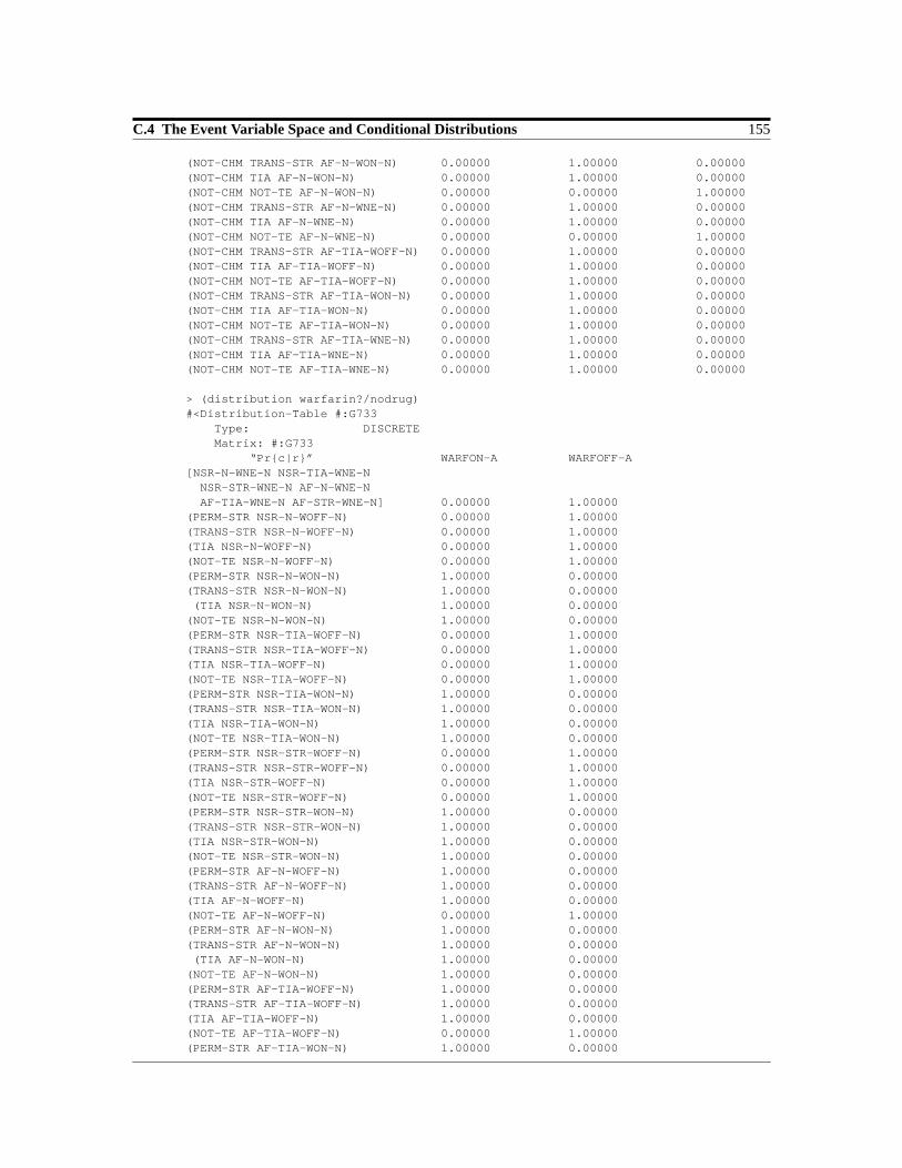
C.4 The Event Variable Space and Conditional Distributions 155
(NOT-CHM TRANS-STR AF-N-WON-N) 0.00000 1.00000 0.00000(NOT-CHM TIA AF-N-WON-N) 0.00000 1.00000 0.00000(NOT-CHM NOT-TE AF-N-WON-N) 0.00000 0.00000 1.00000(NOT-CHM TRANS-STR AF-N-WNE-N) 0.00000 1.00000 0.00000(NOT-CHM TIA AF-N-WNE-N) 0.00000 1.00000 0.00000(NOT-CHM NOT-TE AF-N-WNE-N) 0.00000 0.00000 1.00000(NOT-CHM TRANS-STR AF-TIA-WOFF-N) 0.00000 1.00000 0.00000(NOT-CHM TIA AF-TIA-WOFF-N) 0.00000 1.00000 0.00000(NOT-CHM NOT-TE AF-TIA-WOFF-N) 0.00000 1.00000 0.00000(NOT-CHM TRANS-STR AF-TIA-WON-N) 0.00000 1.00000 0.00000(NOT-CHM TIA AF-TIA-WON-N) 0.00000 1.00000 0.00000(NOT-CHM NOT-TE AF-TIA-WON-N) 0.00000 1.00000 0.00000(NOT-CHM TRANS-STR AF-TIA-WNE-N) 0.00000 1.00000 0.00000(NOT-CHM TIA AF-TIA-WNE-N) 0.00000 1.00000 0.00000(NOT-CHM NOT-TE AF-TIA-WNE-N) 0.00000 1.00000 0.00000
> (distribution warfarin?/nodrug)#<Distribution-Table #:G733 Type: DISCRETE Matrix: #:G733 “Prc|r” WARFON-A WARFOFF-A[NSR-N-WNE-N NSR-TIA-WNE-N NSR-STR-WNE-N AF-N-WNE-N AF-TIA-WNE-N AF-STR-WNE-N] 0.00000 1.00000(PERM-STR NSR-N-WOFF-N) 0.00000 1.00000(TRANS-STR NSR-N-WOFF-N) 0.00000 1.00000(TIA NSR-N-WOFF-N) 0.00000 1.00000(NOT-TE NSR-N-WOFF-N) 0.00000 1.00000(PERM-STR NSR-N-WON-N) 1.00000 0.00000(TRANS-STR NSR-N-WON-N) 1.00000 0.00000 (TIA NSR-N-WON-N) 1.00000 0.00000(NOT-TE NSR-N-WON-N) 1.00000 0.00000(PERM-STR NSR-TIA-WOFF-N) 0.00000 1.00000(TRANS-STR NSR-TIA-WOFF-N) 0.00000 1.00000(TIA NSR-TIA-WOFF-N) 0.00000 1.00000(NOT-TE NSR-TIA-WOFF-N) 0.00000 1.00000(PERM-STR NSR-TIA-WON-N) 1.00000 0.00000(TRANS-STR NSR-TIA-WON-N) 1.00000 0.00000(TIA NSR-TIA-WON-N) 1.00000 0.00000(NOT-TE NSR-TIA-WON-N) 1.00000 0.00000(PERM-STR NSR-STR-WOFF-N) 0.00000 1.00000(TRANS-STR NSR-STR-WOFF-N) 0.00000 1.00000(TIA NSR-STR-WOFF-N) 0.00000 1.00000(NOT-TE NSR-STR-WOFF-N) 0.00000 1.00000(PERM-STR NSR-STR-WON-N) 1.00000 0.00000(TRANS-STR NSR-STR-WON-N) 1.00000 0.00000(TIA NSR-STR-WON-N) 1.00000 0.00000(NOT-TE NSR-STR-WON-N) 1.00000 0.00000(PERM-STR AF-N-WOFF-N) 1.00000 0.00000(TRANS-STR AF-N-WOFF-N) 1.00000 0.00000(TIA AF-N-WOFF-N) 1.00000 0.00000(NOT-TE AF-N-WOFF-N) 0.00000 1.00000(PERM-STR AF-N-WON-N) 1.00000 0.00000(TRANS-STR AF-N-WON-N) 1.00000 0.00000 (TIA AF-N-WON-N) 1.00000 0.00000(NOT-TE AF-N-WON-N) 1.00000 0.00000(PERM-STR AF-TIA-WOFF-N) 1.00000 0.00000(TRANS-STR AF-TIA-WOFF-N) 1.00000 0.00000(TIA AF-TIA-WOFF-N) 1.00000 0.00000(NOT-TE AF-TIA-WOFF-N) 0.00000 1.00000(PERM-STR AF-TIA-WON-N) 1.00000 0.00000

156 C Dynamic Decision Model for the Case Study
(TRANS-STR AF-TIA-WON-N) 1.00000 0.00000(TIA AF-TIA-WON-N) 1.00000 0.00000(NOT-TE AF-TIA-WON-N) 1.00000 0.00000(PERM-STR AF-STR-WOFF-N) 1.00000 0.00000(TRANS-STR AF-STR-WOFF-N) 1.00000 0.00000(TIA AF-STR-WOFF-N) 1.00000 0.00000(NOT-TE AF-STR-WOFF-N) 0.00000 1.00000(PERM-STR AF-STR-WON-N) 1.00000 0.00000(TRANS-STR AF-STR-WON-N) 1.00000 0.00000(TIA AF-STR-WON-N) 1.00000 0.00000(NOT-TE AF-STR-WON-N) 1.00000 0.00000
> (distribution warfarin-ok?/nodrug)#<Distribution-Table #:G731 Type: DISCRETE Matrix: #:G731 “Prc|r” WARFOK-A WARFNE-A[CHM GIB NSR-N-WNE-N NSR-TIA-WNE-N NSR-STR-WNE-N AF-N-WNE-N F-TIA-WNE-N AF-STR-WNE-N] 0.00000 1.00000(NOT-CHM NOT-GIB NSR-N-WOFF-N) 1.00000 0.00000(NOT-CHM NOT-GIB NSR-N-WON-N) 1.00000 0.00000(NOT-CHM NOT-GIB NSR-TIA-WOFF-N) 1.00000 0.00000(NOT-CHM NOT-GIB NSR-TIA-WON-N) 1.00000 0.00000(NOT-CHM NOT-GIB NSR-STR-WOFF-N) 1.00000 0.00000(NOT-CHM NOT-GIB NSR-STR-WON-N) 1.00000 0.00000(NOT-CHM NOT-GIB AF-N-WOFF-N) 1.00000 0.00000(NOT-CHM NOT-GIB AF-N-WON-N) 1.00000 0.00000(NOT-CHM NOT-GIB AF-TIA-WOFF-N) 1.00000 0.00000(NOT-CHM NOT-GIB AF-TIA-WON-N) 1.00000 0.00000(NOT-CHM NOT-GIB AF-STR-WOFF-N) 1.00000 0.00000(NOT-CHM NOT-GIB AF-STR-WON-N) 1.00000 0.00000
;;; Output of different format for this large table.> (distribution state/nodrug)#<Distribution-Table #:G729 Type: DISCRETE Matrix: #:G729 Distribution-Table #:G601
For OUTCOME: NSR-N-WOFFNSR-N-WOFF | (NO-STR-A NSR-A WARFOFF-A WARFOK-A ALIVE-A): 1.00000
For OUTCOME: NSR-N-WONNSR-N-WON | (NO-STR-A NSR-A WARFON-A WARFOK-A ALIVE-A): 1.00000
For OUTCOME: NSR-N-WNENSR-N-WNE | (NO-STR-A NSR-A WARFON-A WARFNE-A ALIVE-A): 1.00000NSR-N-WNE | (NO-STR-A NSR-A WARFOFF-A WARFNE-A ALIVE-A): 1.00000
For OUTCOME: NSR-TIA-WOFFNSR-TIA-WOFF | (TIA-A NSR-A WARFOFF-A WARFOK-A ALIVE-A): 1.00000
For OUTCOME: NSR-TIA-WONNSR-TIA-WON | (TIA-A NSR-A WARFON-A WARFOK-A ALIVE-A): 1.00000
For OUTCOME: NSR-TIA-WNENSR-TIA-WNE | (TIA-A NSR-A WARFON-A WARFNE-A ALIVE-A): 1.00000NSR-TIA-WNE | (TIA-A NSR-A WARFOFF-A WARFNE-A ALIVE-A): 1.00000

C.4 The Event Variable Space and Conditional Distributions 157
For OUTCOME: NSR-STR-WOFFNSR-STR-WOFF | (STR-A NSR-A WARFOFF-A WARFOK-A ALIVE-A): 1.00000
For OUTCOME: NSR-STR-WONNSR-STR-WON | (STR-A NSR-A WARFON-A WARFOK-A ALIVE-A): 1.00000
For OUTCOME: NSR-STR-WNENSR-STR-WNE | (STR-A NSR-A WARFON-A WARFNE-A ALIVE-A): 1.00000NSR-STR-WNE | (STR-A NSR-A WARFOFF-A WARFNE-A ALIVE-A): 1.00000
For OUTCOME: AF-N-WOFFAF-N-WOFF | (NO-STR-A AFIB-A WARFOFF-A WARFOK-A ALIVE-A): 1.00000
For OUTCOME: AF-N-WONAF-N-WON | (NO-STR-A AFIB-A WARFON-A WARFOK-A ALIVE-A): 1.00000
For OUTCOME: AF-N-WNEAF-N-WNE | (NO-STR-A AFIB-A WARFON-A WARFNE-A ALIVE-A): 1.00000AF-N-WNE | (NO-STR-A AFIB-A WARFOFF-A WARFNE-A ALIVE-A): 1.00000
For OUTCOME: AF-TIA-WOFFAF-TIA-WOFF | (TIA-A AFIB-A WARFOFF-A WARFOK-A ALIVE-A): 1.00000
For OUTCOME: AF-TIA-WONAF-TIA-WON | (TIA-A AFIB-A WARFON-A WARFOK-A ALIVE-A): 1.00000
For OUTCOME: AF-TIA-WNEAF-TIA-WNE | (TIA-A AFIB-A WARFON-A WARFNE-A ALIVE-A): 1.00000AF-TIA-WNE | (TIA-A AFIB-A WARFOFF-A WARFNE-A ALIVE-A): 1.00000
For OUTCOME: AF-STR-WOFFAF-STR-WOFF | (STR-A AFIB-A WARFOFF-A WARFOK-A ALIVE-A): 1.00000
For OUTCOME: AF-STR-WONAF-STR-WON | (STR-A AFIB-A WARFON-A WARFOK-A ALIVE-A): 1.00000
For OUTCOME: AF-STR-WNEAF-STR-WNE | (STR-A AFIB-A WARFON-A WARFNE-A ALIVE-A): 1.00000AF-STR-WNE | (STR-A AFIB-A WARFOFF-A WARFNE-A ALIVE-A): 1.00000
For OUTCOME: DEADDEAD | DEAD-A: 1.00000
> ;;; Distributions for action QUINIDINE.
(distribution state-n/quinidine)#<Distribution-Table #:G767 Type: DISCRETE Matrix: #:G767
NSR-N-WOFF-N 0.05556 NSR-N-WON-N 0.05556 NSR-N-WNE-N 0.05556 NSR-TIA-WOFF-N 0.05556 NSR-TIA-WON-N 0.05556 NSR-TIA-WNE-N 0.05556 NSR-STR-WOFF-N 0.05556 NSR-STR-WON-N 0.05556 NSR-STR-WNE-N 0.05556 AF-N-WOFF-N 0.05556 AF-N-WON-N 0.05556

158 C Dynamic Decision Model for the Case Study
AF-N-WNE-N 0.05556 AF-TIA-WOFF-N 0.05556 AF-TIA-WON-N 0.05556 AF-TIA-WNE-N 0.05556 AF-STR-WOFF-N 0.05556 AF-STR-WON-N 0.05556 AF-STR-WNE-N 0.05556
> (distribution ?die/quinidine)#<Distribution-Table #:G765 Type: DISCRETE Matrix: #:G765 “Prc|r” DIE NOT-DIE NSR-N-WOFF-N PMUSUM-QUIN PMUSUM-QUIN-COMP NSR-N-WON-N PMUSUM-QUIN PMUSUM-QUIN-COMP NSR-N-WNE-N PMUSUM-QUIN PMUSUM-QUIN-COMP NSR-TIA-WOFF-N PMUSUM-QUIN PMUSUM-QUIN-COMP NSR-TIA-WON-N PMUSUM-QUIN PMUSUM-QUIN-COMP NSR-TIA-WNE-N PMUSUM-QUIN PMUSUM-QUIN-COMP NSR-STR-WOFF-N PMUSUM-QUIN PMUSUM-QUIN-COMP NSR-STR-WON-N PMUSUM-QUIN PMUSUM-QUIN-COMP NSR-STR-WNE-N PMUSUM-QUIN PMUSUM-QUIN-COMP AF-N-WOFF-N PMUSUM-QUIN PMUSUM-QUIN-COMP AF-N-WON-N PMUSUM-QUIN PMUSUM-QUIN-COMP AF-N-WNE-N PMUSUM-QUIN PMUSUM-QUIN-COMP AF-TIA-WOFF-N PMUSUM-QUIN PMUSUM-QUIN-COMP AF-TIA-WON-N PMUSUM-QUIN PMUSUM-QUIN-COMP AF-TIA-WNE-N PMUSUM-QUIN PMUSUM-QUIN-COMP AF-STR-WOFF-N PMUSUM-QUIN PMUSUM-QUIN-COMP AF-STR-WON-N PMUSUM-QUIN PMUSUM-QUIN-COMP AF-STR-WNE-N PMUSUM-QUIN PMUSUM-QUIN-COMP
> (distribution ?te/quinidine)#<Distribution-Table #:G761 Type: DISCRETE Matrix: #:G761
“Prc|r” PERM-STR TRANS-STR TIA NOT-TE NSR-N-WOFF-N PPERM-STR PTRANS-STR PTIA (- 1 PEMB) NSR-N-WON-N PPERM-STR-W PTRANS-STR-W PTIA-W (- 1 PEMB-WARF) NSR-N-WNE-N PPERM-STR PTRANS-STR PTIA (- 1 PEMB) NSR-TIA-WOFF-N PPERM-STR-S PTRANS-STR-S PTIA-S (- 1 PEMB-STR) NSR-TIA-WON-N PPERM-STR-SW PTRANS-STR-SW PTIA-SW (- 1 PEMB-STR-WARF) NSR-TIA-WNE-N PPERM-STR-S PTRANS-STR-S PTIA-S (- 1 PEMB-STR) NSR-STR-WOFF-N PPERM-STR-S PTRANS-STR-S PTIA-S (- 1 PEMB-STR) NSR-STR-WON-N PPERM-STR-SW PTRANS-STR-SW PTIA-SW (- 1 PEMB-STR-WARF) NSR-STR-WNE-N PPERM-STR-S PTRANS-STR-S PTIA-S (- 1 PEMB-STR) AF-N-WOFF-N PPERM-STR-A PTRANS-STR-A PTIA-A (- 1 PEMB-AF) AF-N-WON-N PPERM-STR-AW PTRANS-STR-AW PTIA-AW (- 1 PEMB-AF-WARF) AF-N-WNE-N PPERM-STR-A PTRANS-STR-A PTIA-A (- 1 PEMB-AF) AF-TIA-WOFF-N PPERM-STR-AS PTRANS-STR-AS PTIA-AS (- 1 PEMB-AF-STR) AF-TIA-WON-N PPERM-STR-ALL PTRANS-STR-ALL PTIA-ALL (- 1 PEMB-ALL) AF-TIA-WNE-N PPERM-STR-AS PTRANS-STR-AS PTIA-AS (- 1 PEMB-AF-STR) AF-STR-WOFF-N PPERM-STR-AS PTRANS-STR-AS PTIA-AS (- 1 PEMB-AF-STR) AF-STR-WON-N PPERM-STR-ALL PTRANS-STR-ALL PTIA-ALL (- 1 PEMB-ALL) AF-STR-WNE-N PPERM-STR-AS PTRANS-STR-AS PTIA-AS (- 1 PEMB-AF-STR)

C.4 The Event Variable Space and Conditional Distributions 159
> (distribution ?cerehem/quinidine)#<Distribution-Table #:G773 Type: DISCRETE Matrix: #:G773 “Prc|r” CHM NOT-CHM NSR-N-WOFF-N PCEREHEM (- 1 PCEREHEM) NSR-N-WON-N PCEREHEM-WARF PCEREHEM-WARF-COMP NSR-N-WNE-N PCEREHEM (- 1 PCEREHEM) NSR-TIA-WOFF-N PCEREHEM (- 1 PCEREHEM) NSR-TIA-WON-N PCEREHEM-WARF PCEREHEM-WARF-COMP NSR-TIA-WNE-N PCEREHEM (- 1 PCEREHEM) NSR-STR-WOFF-N PCEREHEM (- 1 PCEREHEM) NSR-STR-WON-N PCEREHEM-WARF PCEREHEM-WARF-COMP NSR-STR-WNE-N PCEREHEM (- 1 PCEREHEM) AF-N-WOFF-N PCEREHEM (- 1 PCEREHEM) AF-N-WON-N PCEREHEM-WARF PCEREHEM-WARF-COMP AF-N-WNE-N PCEREHEM (- 1 PCEREHEM) AF-TIA-WOFF-N PCEREHEM (- 1 PCEREHEM) AF-TIA-WON-N PCEREHEM-WARF PCEREHEM-WARF-COMP AF-TIA-WNE-N PCEREHEM (- 1 PCEREHEM) AF-STR-WOFF-N PCEREHEM (- 1 PCEREHEM) AF-STR-WON-N PCEREHEM-WARF PCEREHEM-WARF-COMP AF-STR-WNE-N PCEREHEM (- 1 PCEREHEM)
> (distribution ?gi-bleeding/quinidine)#<Distribution-Table #:G757 Type: DISCRETE Matrix: #:G757 “Prc|r” GIB NOT-GIB NSR-N-WOFF-N PGIB (- 1 PGIB) NSR-N-WON-N PGIB-WARF PGIB-WARF-COMP NSR-N-WNE-N PGIB (- 1 PGIB) NSR-TIA-WOFF-N PGIB (- 1 PGIB) NSR-TIA-WON-N PGIB-WARF PGIB-WARF-COMP NSR-TIA-WNE-N PGIB (- 1 PGIB) NSR-STR-WOFF-N PGIB (- 1 PGIB) NSR-STR-WON-N PGIB-WARF PGIB-WARF-COMP NSR-STR-WNE-N PGIB (- 1 PGIB) AF-N-WOFF-N PGIB (- 1 PGIB) AF-N-WON-N PGIB-WARF PGIB-WARF-COMP AF-N-WNE-N PGIB (- 1 PGIB) AF-TIA-WOFF-N PGIB (- 1 PGIB) AF-TIA-WON-N PGIB-WARF PGIB-WARF-COMP AF-TIA-WNE-N PGIB (- 1 PGIB) AF-STR-WOFF-N PGIB (- 1 PGIB) AF-STR-WON-N PGIB-WARF PGIB-WARF-COMP AF-STR-WNE-N PGIB (- 1 PGIB)
> (distribution ?die-te/quinidine)#<Distribution-Table #:G751 Type: DISCRETE Matrix: #:G751 “Prc|r” DIE-TE NOT-DIE-TE PERM-STR PDSTROKE (- 1 PDSTROKE) TRANS-STR PDSTROKE (- 1 PDSTROKE) TIA 0.00000 1.00000 NOT-TE 0.00000 1.00000

160 C Dynamic Decision Model for the Case Study
> (distribution ?die-cerehem/quinidine)#<Distribution-Table #:G759 Type: DISCRETE Matrix: #:G759 “Prc|r” DIE-CHM NOT-DIE-CHM CHM PDIECHM (- 1 PDIECHM) NOT-CHM 0.00000 1.00000
> (distribution ?die-gi-bleeding/quinidine)#<Distribution-Table #:G771 Type: DISCRETE Matrix: #:G771 “Prc|r” DIE-GIB NOT-DIE-GIB GIB PDIEGIB (- 1 PDIEGIB) NOT-GIB 0.00000 1.00000
> (distribution afib?/quinidine)#<Distribution-Table #:G753 Type: DISCRETE Matrix: #:G753 “Prc|r” NSR-A AFIB-A NSR-N-WOFF-N (- 1 PAFIB-QUIN) PAFIB-QUIN NSR-N-WON-N (- 1 PAFIB-QUIN) PAFIB-QUIN NSR-N-WNE-N (- 1 PAFIB-QUIN) PAFIB-QUIN NSR-TIA-WOFF-N (- 1 PAFIB-QUIN) PAFIB-QUIN NSR-TIA-WON-N (- 1 PAFIB-QUIN) PAFIB-QUIN NSR-TIA-WNE-N (- 1 PAFIB-QUIN) PAFIB-QUIN NSR-STR-WOFF-N (- 1 PAFIB-QUIN) PAFIB-QUIN NSR-STR-WON-N (- 1 PAFIB-QUIN) PAFIB-QUIN NSR-STR-WNE-N (- 1 PAFIB-QUIN) PAFIB-QUIN AF-N-WOFF-N (- 1 PAFIB-QUIN-STAY) PAFIB-QUIN-STAY AF-N-WON-N (- 1 PAFIB-QUIN-STAY) PAFIB-QUIN-STAY AF-N-WNE-N (- 1 PAFIB-QUIN-STAY) PAFIB-QUIN-STAY AF-TIA-WOFF-N (- 1 PAFIB-QUIN-STAY) PAFIB-QUIN-STAY AF-TIA-WON-N (- 1 PAFIB-QUIN-STAY) PAFIB-QUIN-STAY AF-TIA-WNE-N (- 1 PAFIB-QUIN-STAY) PAFIB-QUIN-STAY AF-STR-WOFF-N (- 1 PAFIB-QUIN-STAY) PAFIB-QUIN-STAY AF-STR-WON-N (- 1 PAFIB-QUIN-STAY) PAFIB-QUIN-STAY AF-STR-WNE-N (- 1 PAFIB-QUIN-STAY) PAFIB-QUIN-STAY
> (distribution status?/quinidine)#<Distribution-Table #:G775 Type: DISCRETE Matrix: #:G775 “Prc|r” ALIVE-A DEAD-A[DIE DIE-GIB DIE-CHM DIE-TE] 0.00000 1.00000(NOT-DIE NOT-DIE-GIB NOT-DIE-CHM NOT-DIE-TE) 1.00000 0.00000
> (distribution stroke?/quinidine)#<Distribution-Table #:G769 Type: DISCRETE Matrix: #:G769 “Prc|r” STR-A TIA-A NO-STR-A[CHM PERM-STR NSR-STR-WOFF-N NSR-STR-WON-N NSR-STR-WNE-N AF-STR-WOFF-N AF-STR-WON-N AF-STR-WNE-N] 1.00000 0.00000 0.00000(NOT-CHM TRANS-STR NSR-N-WOFF-N) 0.00000 1.00000 0.00000(NOT-CHM TIA NSR-N-WOFF-N) 0.00000 1.00000 0.00000(NOT-CHM NOT-TE NSR-N-WOFF-N) 0.00000 0.00000 1.00000(NOT-CHM TRANS-STR NSR-N-WON-N) 0.00000 1.00000 0.00000

C.4 The Event Variable Space and Conditional Distributions 161
(NOT-CHM TIA NSR-N-WON-N) 0.00000 1.00000 0.00000(NOT-CHM NOT-TE NSR-N-WON-N) 0.00000 0.00000 1.00000(NOT-CHM TRANS-STR NSR-N-WNE-N) 0.00000 1.00000 0.00000(NOT-CHM TIA NSR-N-WNE-N) 0.00000 1.00000 0.00000(NOT-CHM NOT-TE NSR-N-WNE-N) 0.00000 0.00000 1.00000(NOT-CHM TRANS-STR NSR-TIA-WOFF-N) 0.00000 1.00000 0.00000(NOT-CHM TIA NSR-TIA-WOFF-N) 0.00000 1.00000 0.00000(NOT-CHM NOT-TE NSR-TIA-WOFF-N) 0.00000 1.00000 0.00000(NOT-CHM TRANS-STR NSR-TIA-WON-N) 0.00000 1.00000 0.00000(NOT-CHM TIA NSR-TIA-WON-N) 0.00000 1.00000 0.00000(NOT-CHM NOT-TE NSR-TIA-WON-N) 0.00000 1.00000 0.00000(NOT-CHM TRANS-STR NSR-TIA-WNE-N) 0.00000 1.00000 0.00000(NOT-CHM TIA NSR-TIA-WNE-N) 0.00000 1.00000 0.00000(NOT-CHM NOT-TE NSR-TIA-WNE-N) 0.00000 1.00000 0.00000(NOT-CHM TRANS-STR AF-N-WOFF-N) 0.00000 1.00000 0.00000(NOT-CHM TIA AF-N-WOFF-N) 0.00000 1.00000 0.00000(NOT-CHM NOT-TE AF-N-WOFF-N) 0.00000 0.00000 1.00000(NOT-CHM TRANS-STR AF-N-WON-N) 0.00000 1.00000 0.00000(NOT-CHM TIA AF-N-WON-N) 0.00000 1.00000 0.00000(NOT-CHM NOT-TE AF-N-WON-N) 0.00000 0.00000 1.00000(NOT-CHM TRANS-STR AF-N-WNE-N) 0.00000 1.00000 0.00000(NOT-CHM TIA AF-N-WNE-N) 0.00000 1.00000 0.00000(NOT-CHM NOT-TE AF-N-WNE-N) 0.00000 0.00000 1.00000(NOT-CHM TRANS-STR AF-TIA-WOFF-N) 0.00000 1.00000 0.00000(NOT-CHM TIA AF-TIA-WOFF-N) 0.00000 1.00000 0.00000(NOT-CHM NOT-TE AF-TIA-WOFF-N) 0.00000 1.00000 0.00000(NOT-CHM TRANS-STR AF-TIA-WON-N) 0.00000 1.00000 0.00000(NOT-CHM TIA AF-TIA-WON-N) 0.00000 1.00000 0.00000(NOT-CHM NOT-TE AF-TIA-WON-N) 0.00000 1.00000 0.00000(NOT-CHM TRANS-STR AF-TIA-WNE-N) 0.00000 1.00000 0.00000(NOT-CHM TIA AF-TIA-WNE-N) 0.00000 1.00000 0.00000(NOT-CHM NOT-TE AF-TIA-WNE-N) 0.00000 1.00000 0.00000
> (distribution warfarin?/quinidine)#<Distribution-Table #:G749 Type: DISCRETE Matrix: #:G749 “Prc|r” WARFON-A WARFOFF-A[NSR-N-WNE-N NSR-TIA-WNE-N NSR-STR-WNE-N AF-N-WNE-N AF-TIA-WNE-N AF-STR-WNE-N] 0.00000 1.00000(PERM-STR NSR-N-WOFF-N) 0.00000 1.00000(TRANS-STR NSR-N-WOFF-N) 0.00000 1.00000(TIA NSR-N-WOFF-N) 0.00000 1.00000(NOT-TE NSR-N-WOFF-N) 0.00000 1.00000(PERM-STR NSR-N-WON-N) 1.00000 0.00000(TRANS-STR NSR-N-WON-N) 1.00000 0.00000(TIA NSR-N-WON-N) 1.00000 0.00000(NOT-TE NSR-N-WON-N) 1.00000 0.00000(PERM-STR NSR-TIA-WOFF-N) 0.00000 1.00000(TRANS-STR NSR-TIA-WOFF-N) 0.00000 1.00000(TIA NSR-TIA-WOFF-N) 0.00000 1.00000(NOT-TE NSR-TIA-WOFF-N) 0.00000 1.00000(PERM-STR NSR-TIA-WON-N) 1.00000 0.00000(TRANS-STR NSR-TIA-WON-N) 1.00000 0.00000(TIA NSR-TIA-WON-N) 1.00000 0.00000(NOT-TE NSR-TIA-WON-N) 1.00000 0.00000(PERM-STR NSR-STR-WOFF-N) 0.00000 1.00000(TRANS-STR NSR-STR-WOFF-N) 0.00000 1.00000(TIA NSR-STR-WOFF-N) 0.00000 1.00000(NOT-TE NSR-STR-WOFF-N) 0.00000 1.00000

162 C Dynamic Decision Model for the Case Study
(PERM-STR NSR-STR-WON-N) 1.00000 0.00000(TRANS-STR NSR-STR-WON-N) 1.00000 0.00000(TIA NSR-STR-WON-N) 1.00000 0.00000(NOT-TE NSR-STR-WON-N) 1.00000 0.00000(PERM-STR AF-N-WOFF-N) 1.00000 0.00000(TRANS-STR AF-N-WOFF-N) 1.00000 0.00000(TIA AF-N-WOFF-N) 1.00000 0.00000(NOT-TE AF-N-WOFF-N) 0.00000 1.00000(PERM-STR AF-N-WON-N) 1.00000 0.00000(TRANS-STR AF-N-WON-N) 1.00000 0.00000 (TIA AF-N-WON-N) 1.00000 0.00000(NOT-TE AF-N-WON-N) 1.00000 0.00000(PERM-STR AF-TIA-WOFF-N) 1.00000 0.00000(TRANS-STR AF-TIA-WOFF-N) 1.00000 0.00000(TIA AF-TIA-WOFF-N) 1.00000 0.00000(NOT-TE AF-TIA-WOFF-N) 0.00000 1.00000(PERM-STR AF-TIA-WON-N) 1.00000 0.00000(TRANS-STR AF-TIA-WON-N) 1.00000 0.00000(TIA AF-TIA-WON-N) 1.00000 0.00000(NOT-TE AF-TIA-WON-N) 1.00000 0.00000(PERM-STR AF-STR-WOFF-N) 1.00000 0.00000(TRANS-STR AF-STR-WOFF-N) 1.00000 0.00000(TIA AF-STR-WOFF-N) 1.00000 0.00000(NOT-TE AF-STR-WOFF-N) 0.00000 1.00000(PERM-STR AF-STR-WON-N) 1.00000 0.00000(TRANS-STR AF-STR-WON-N) 1.00000 0.00000(TIA AF-STR-WON-N) 1.00000 0.00000(NOT-TE AF-STR-WON-N) 1.00000 0.00000
> (distribution warfarin-ok?/quinidine)#<Distribution-Table #:G763 Type: DISCRETE Matrix: #:G763 “Prc|r” WARFOK-A WARFNE-A[CHM GIB NSR-N-WNE-N NSR-TIA-WNE-N NSR-STR-WNE-N AF-N-WNE-N AF-TIA-WNE-N AF-STR-WNE-N] 0.00000 1.00000(NOT-CHM NOT-GIB NSR-N-WOFF-N) 1.00000 0.00000(NOT-CHM NOT-GIB NSR-N-WON-N) 1.00000 0.00000(NOT-CHM NOT-GIB NSR-TIA-WOFF-N) 1.00000 0.00000(NOT-CHM NOT-GIB NSR-TIA-WON-N) 1.00000 0.00000(NOT-CHM NOT-GIB NSR-STR-WOFF-N) 1.00000 0.00000(NOT-CHM NOT-GIB NSR-STR-WON-N) 1.00000 0.00000(NOT-CHM NOT-GIB AF-N-WOFF-N) 1.00000 0.00000(NOT-CHM NOT-GIB AF-N-WON-N) 1.00000 0.00000(NOT-CHM NOT-GIB AF-TIA-WOFF-N) 1.00000 0.00000(NOT-CHM NOT-GIB AF-TIA-WON-N) 1.00000 0.00000(NOT-CHM NOT-GIB AF-STR-WOFF-N) 1.00000 0.00000(NOT-CHM NOT-GIB AF-STR-WON-N) 1.00000 0.00000
;;; Different output format for this large table.> (distribution state/quinidine)#<Distribution-Table #:G755 Type: DISCRETE Matrix: #:G755 Distribution-Table #:G630
For OUTCOME: NSR-N-WOFFNSR-N-WOFF | (NO-STR-A NSR-A WARFOFF-A WARFOK-A ALIVE-A): 1.00000

C.4 The Event Variable Space and Conditional Distributions 163
For OUTCOME: NSR-N-WONNSR-N-WON | (NO-STR-A NSR-A WARFON-A WARFOK-A ALIVE-A): 1.00000
For OUTCOME: NSR-N-WNENSR-N-WNE | (NO-STR-A NSR-A WARFON-A WARFNE-A ALIVE-A): 1.00000NSR-N-WNE | (NO-STR-A NSR-A WARFOFF-A WARFNE-A ALIVE-A): 1.00000
For OUTCOME: NSR-TIA-WOFFNSR-TIA-WOFF | (TIA-A NSR-A WARFOFF-A WARFOK-A ALIVE-A): 1.00000
For OUTCOME: NSR-TIA-WONNSR-TIA-WON | (TIA-A NSR-A WARFON-A WARFOK-A ALIVE-A): 1.00000
For OUTCOME: NSR-TIA-WNENSR-TIA-WNE | (TIA-A NSR-A WARFON-A WARFNE-A ALIVE-A): 1.00000NSR-TIA-WNE | (TIA-A NSR-A WARFOFF-A WARFNE-A ALIVE-A): 1.00000
For OUTCOME: NSR-STR-WOFFNSR-STR-WOFF | (STR-A NSR-A WARFOFF-A WARFOK-A ALIVE-A): 1.00000
For OUTCOME: NSR-STR-WONNSR-STR-WON | (STR-A NSR-A WARFON-A WARFOK-A ALIVE-A): 1.00000
For OUTCOME: NSR-STR-WNENSR-STR-WNE | (STR-A NSR-A WARFON-A WARFNE-A ALIVE-A): 1.00000NSR-STR-WNE | (STR-A NSR-A WARFOFF-A WARFNE-A ALIVE-A): 1.00000
For OUTCOME: AF-N-WOFFAF-N-WOFF | (NO-STR-A AFIB-A WARFOFF-A WARFOK-A ALIVE-A): 1.00000
For OUTCOME: AF-N-WONAF-N-WON | (NO-STR-A AFIB-A WARFON-A WARFOK-A ALIVE-A): 1.00000
For OUTCOME: AF-N-WNEAF-N-WNE | (NO-STR-A AFIB-A WARFON-A WARFNE-A ALIVE-A): 1.00000AF-N-WNE | (NO-STR-A AFIB-A WARFOFF-A WARFNE-A ALIVE-A): 1.00000
For OUTCOME: AF-TIA-WOFFAF-TIA-WOFF | (TIA-A AFIB-A WARFOFF-A WARFOK-A ALIVE-A): 1.00000
For OUTCOME: AF-TIA-WONAF-TIA-WON | (TIA-A AFIB-A WARFON-A WARFOK-A ALIVE-A): 1.00000
For OUTCOME: AF-TIA-WNEAF-TIA-WNE | (TIA-A AFIB-A WARFON-A WARFNE-A ALIVE-A): 1.00000AF-TIA-WNE | (TIA-A AFIB-A WARFOFF-A WARFNE-A ALIVE-A): 1.00000
For OUTCOME: AF-STR-WOFFAF-STR-WOFF | (STR-A AFIB-A WARFOFF-A WARFOK-A ALIVE-A): 1.00000
For OUTCOME: AF-STR-WONAF-STR-WON | (STR-A AFIB-A WARFON-A WARFOK-A ALIVE-A): 1.00000
For OUTCOME: AF-STR-WNEAF-STR-WNE | (STR-A AFIB-A WARFON-A WARFNE-A ALIVE-A): 1.00000AF-STR-WNE | (STR-A AFIB-A WARFOFF-A WARFNE-A ALIVE-A): 1.00000
For OUTCOME: DEADDEAD | DEAD-A: 1.00000

164 C Dynamic Decision Model for the Case Study
C.5 The Transition Values
The following Common Lisp code is used to specify the transition values once thetransitions are defined. The transition values constitute the bonus componentsin the value functions . The transition value definitions can be subject to sen-sitivity analysis as other numerical parameters. The definitions are as follows:
• Short term morbidities are defined for stroke, transient ischemic attack, andbleeding.
• If a transition is made to a different state where any of the above events areindicated, the short term morbidities are deducted accordingly.
• If a transition is made to the same state with any of the above events exceptstroke, the corresponding short term morbidity multiplied by a small factor of0.05 is deducted.
• If a transition is made to the same state with stroke, the corresponding shortterm morbidity multiplied by a slightly larger factor of 0.25 is deducted. Weassume that a stroke has more serious consequences than the other events.
;;; Full negative bonus for first indication. Factored negative bonus for repeated;;; indications.
(defun load-transition-values5 (action) (let ((n-set (list nsr-n-woff nsr-n-won af-n-woff af-n-won)) (tia-set (list nsr-tia-woff nsr-tia-won af-tia-woff af-tia-won )) (str-set (list nsr-str-woff nsr-str-won af-str-woff af-str-won)) (n-ne-set (list nsr-n-wne af-n-wne)) (tia-ne-set (list nsr-tia-wne af-tia-wne)) (str-ne-set (list nsr-str-wne af-str-wne)))
(set-transition-values action n-set n-ne-set (- stmGIB))
(set-transition-values action n-set tia-set (- stmTIA)) (set-transition-values action n-set tia-ne-set
(- (+ stmTIA stmGIB))) (set-transition-values action n-set str-set
(- (- stmSTROKE (- 1 Ustroke)))) (set-transition-values action n-set str-ne-set
(- (+ (- stmSTROKE (- 1 Ustroke)) stmGIB)))
(set-transition-values action n-ne-set n-ne-set (- (* 0.05 stmGIB)))
(set-transition-values action n-ne-set tia-ne-set (- (+ stmTIA (* 0.05 stmGIB))))
(set-transition-values action n-ne-set str-ne-set (- (+ (- stmSTROKE (- 1 Ustroke))
(* 0.05 stmGIB))))
(set-transition-values action tia-set tia-set (- (* 0.05 stmTIA))) (set-transition-values action tia-set tia-ne-set
(- (+ (* 0.05 stmTIA) stmGIB))) (set-transition-values action tia-set str-set
(- (- stmSTROKE (- 1 Ustroke)))) (set-transition-values action tia-set str-ne-set
(- (+ (- stmSTROKE (- 1 Ustroke)) stmGIB)))
bijvi .( )

C.6 Solution and Analysis 165
(set-transition-values action tia-ne-set tia-ne-set (- (+ (* 0.05 stmTIA) (* 0.05 stmGIB))))
(set-transition-values action tia-ne-set str-ne-set (- (+ (- stmSTROKE (- 1 Ustroke)) (* 0.05 stmGIB))))
(set-transition-values action str-set str-set (- (* 0.25 (- stmSTROKE (- 1 Ustroke)))))
(set-transition-values action str-set str-ne-set (- (+ (* 0.25 (- stmSTROKE (- 1 Ustroke))) stmGIB)))
(set-transition-values action str-ne-set str-ne-set (- (+ (* 0.25 (- stmSTROKE (- 1 Ustroke))) (* 0.05 stmGIB))))))
C.6 Solution and Analysis
Recall that the two clinical questions addressed in the case study are:
Problem 1: Quinidine decreases the proportion of time that the patient spends inAF. Does this decrease his risk of embolic complications enough to justify theincreased risk of sudden death?
Problem 2: What is the optimal course of treatment in the next five years, takinginto account the varying relative risk of bleeding for warfarin with respect to theduration of treatment?
Solution and Analysis of Long-Term Discriminatory Problem
The solution produced by the Markov value iteration solver for discriminatoryproblems is a set of two policies corresponding to the four strategies considered;each policy includes the expected value achievable in all possible starting statesfor all possible decision stages. Assuming that the patient is initially in either stateNSR-N-WOFF or stateAF-N-WOFF. He has a probability of 0.25 to be in atrial fibril-lation, with no thromboembolization history, and not on warfarin at the beginningof the decision horizon. The solution to the first clinical question is detailed inTable C.2. The solution suggests that Quinidine does not decrease the risk ofembolic complications enough to justify the increased risk of sudden death.Although not shown here, similar answers with respect to different starting statescan also be directly derived from the policies information produced by theDYNAMO solver.

166 C Dynamic Decision Model for the Case Study
Table C.2 Solution to long-term discriminatory problem in case study.
Sensitivity analysis on some of the numerical parameters shows that the War-farin strategy dominates except in the following conditions.
The None strategy,i.e., administer warfarin only when indicated and stop whennecessary, becomes the preferred choice under three circumstances: First, when thetherapeutic efficacy of warfarin on preventing thromboembolism falls below 47%,where the efficacy is calculated by:
.
Second, when the complication risks associated with warfarin are very serious, aswhen the relative risk of bleeding exceeds 3.76 (50% increase from base case). therisk of cerebral hemorrhage exceeds 0.0017 (200%), and the risk of gastro-intesti-nal bleeding exceeds 0.015 (150%). Third, when the risk of thromboembolizationis very low, as when the rate of thromboembolization falls below 0.0068 (27%decrease from base case).
The Quinidine strategy becomes the preferred choice only when the excessmortality rate for Quinidine falls below 0.0005 (96% decrease from base case).
Solution and Analysis of Short-Term Optimization Problem
The solution produced by the semi-Markov value iteration solver for optimizationproblems is an optimal policy indicating the optimal expected value achievable inall possible starting states for all possible decision stages. Assuming that thepatient is initially in either stateNSR-N-WOFF or stateAF-N-WOFF. He has a proba-bility of 0.25 to be in atrial fibrillation, with no thromboembolization history, andnot on warfarin at the beginning of the decision horizon. The solution to the secondclinical question is partially detailed in Table C.3. In the table, the unit of the deci-sion stages are in months. The notation “N” indicates the None strategy; the nota-tion “W” indicates the Warfarin strategy. Recall that the decision stage 60 is attime 0.
StrategyQALY
(600 stages)RelativeValue
None 22.2664 -0.3594
Warfarin 22.6258 0
Quinidine 19.3532 -3.2726
Both 19.3781 -3.2477
Efficacy 1 Relative risk−=

C.6 Solution and Analysis 167
The solution shows that the strategy that administers only warfarin initially isthe preferred strategy up to 8 months. After 8 months, if the patient remains in thesame condition, the strategy that does not administer any drug initially is preferred.Again, although not shown here, similar answers with respect to different startingstates can also be directly derived from the policies information produced by theDYNAMO solver. This would allow an optimal treatment course be derived accord-ing to the varying condition of the patient,e.g., what is the best treatment strategya year from now, if he suffers a stroke in the first 3 months and a bleeding episodein the seventh month?
Table C.3 Partial solution to short-term optimization problem.
Sensitivity analysis on some of the numerical parameters shows that the War-farin strategy becomes the preferred strategy over more decision stages when therisk of thromboembolization increases or when the relative risk of bleeding forwarfarin decreases. The same pattern is also observed with waiting time functionsfor the states affected by warfarin that lessen its adverse effects. In the base case,for instance, a patient is more likely to leave his current state sooner, when theprobability of bleeding due to warfarin is higher, than later, when the probability ofbleeding due to warfarin is lower. The adverse effects of warfarin are lessened ifthe patient is equally likely to leave his current state sooner or later.
StageQALY/Strategy
StageQALY/Strategy
5 0.37389 N 35 2.80835 N
10 0.78636 N 40 3.20565 N
15 1.19594 N 45 3.60087 N
20 1.60278 N 50 3.99412 N
25 2.00703 N 55 4.39177 W
30 2.40885 N 60 4.78974 W

168 C Dynamic Decision Model for the Case Study

169
D Glossary
This glossary contains a list of simplified medical concepts from [Bantam, 1990]and [Taber, 1989]. Cross-references within the glossary are initalic.
AnginaA sense of suffocation or suffocating pain.
Antiarrhythmic agentA drug that controls or prevents cardiac arrhythmias or irregular heartbeats.
AnticoagulantAn agent that prevents the clotting of blood. It is used to prevent the formationof blood clots or to break up clots in blood vessels in conditions such asthrom-bosis andembolism.
AtherosclerosisA disease of the arteries in which fatty plaques develop on their inner walls,with eventual obstruction of blood flow.
Cerebral hemorrhageBleeding from a cerebral artery into the tissue of the brain.
Chronic ischemic heart diseaseHeart disease of gradual onset that limits blood supply to the heart muscles.
Coronary artery bypass graftA surgical procedure that establishes a shunt that permits blood to travel fromthe aorta to a branch of the coronary artery at a point past an obstruction.
EmbolismThe condition in which a mass of material such as blood clot becomes lodgedin an artery and obstructs its blood flow.

170 D Glossary
GangreneDeath of tissue, usually due to deficient or absent blood supply.
Gastrointestinal bleedingBleeding in the stomach and the intestines.
Myocardial infarctionHeart attack. Death of a segment of heart muscle, which follows interruption ofits blood supply.
Percutaneous transluminal coronary angioplastyA method of treating localized coronary artery narrowing by applying a specialcatheter with a cylindrical balloon that surrounds a portion of it. Inflation of theballoon dilates the narrowed vessel.
Paroxysmal atrial fibrillationA kind of cardiac arrhymia or abnormal heartbeat of sudden onset. It resultsfrom irregular and rapid randomized contractions of the atria working indepen-dently of the ventricles.
RestenosisThe reccurrence of a stenosis or the condition of constriction or narrowing of apassage or orifice.
QuinidineAn antiarrhythmic agent that slows down the activity of the heart and isadministered by mouth to control abnormal and increased heart rhythm.
Sinus rhythmThe normal cardiac rhythm or heartbeat rate.
ThromboembolismAn embolism; the blocking of a blood vessel by a blood clot or thrombus thathas become detached from its site of formation.
ThrombosisThe formation, development, or existence of a blood clot or thrombus withinthe vascular system.
WarfarinAn anticoagulant used mainly to treat coronary or venousthrombosis to reducethe risk ofembolism. It is given by mouth or injection.
171
References
Bantam (1990). The bantam medical dictionary, revised edition. Bantam Books.
Beck, J. R. and Pauker, S. G. (1983). The Markov process in medical prognosis.Medical Decision Making, 3:419–458.
Bellman, R. A. (1957).Dynamic Programming. Princeton University Press, Princ-eton, NJ.
Bertsekas, D. P. (1987).Dynamic Programming: Deterministic and StochasticModels. Prentice-Hall, Englewood Cliffs, NJ.
Berzuini, C., Bellazzi, R., and Quaglini, S. (1989). Temporal reasoning with prob-abilities. InProceedings of the Fifth Workshop on Uncertainty in Artificial Intelli-gence, pages 14–21. Association for Uncertainty in Artificial Intelligence.
Breese, J. S. (1992). Construction of belief and decision networks.ComputationalIntelligence, 8:624–647.
Chan, B. Y. and Shachter, R. D. (1992). Structural controllability and observabilityin influence diagrams. In Dubois, D., Wellman, M. P., D’Ambrosio, B. D., andSmets, P., editors,Uncertainty in Artificial Intelligence: Proceedings of the EighthConference, pages 25–32, San Mateo, CA. Morgan Kaufmann.
Chapman, D. (1987). Planning for conjunctive goals.Artificial Intelligence,32:333–377.
Clemen, R. T. (1991).Making Hard Decisions: An Introduction to Decision Analy-sis. PWS-KENT, Boston, MA.
Cooper, G. F. (1990). The computational complexity of probabilistic inferenceusing Bayesian belief networks.Artificial Intelligence, 42(2-3):393–405.
Dean, T. (1994). Decision-theoretic planning and markov decision processes. Sub-mitted for publication.
Dean, T., Kaelbling, L. P., Kirman, J., and Nicholson, A. (1993a). Deliberationscheduling for time-critical sequential decision making. In Heckerman, D. andMamdami, A., editors,Uncertainty in Artificial Intelligence: Proceedings of theNinth Conference, pages 309–316, San Mateo, CA. Morgan Kaufmann.
Dean, T., Kaelbling, L. P., Kirman, J., and Nicholson, A. (1993b). Planning withdeadlines in stochastic domains. InProceedings of the Eleventh National Confer-ence on Artificial Intelligence, pages 574–579.

172 References
Dean, T., Kriman, J., and Kanazawa, K. (1992). Probabilistic network representa-tions of continuous-time stochastic processes for applications in planning and con-trol. In Proceedings of the First International Conference on AI Planning Systems.
Dean, T. L. and Wellman, M. P. (1991).Planning and Control. Morgan Kaufmann,San Mateo, CA.
Deardon, R. and Boutilier, C. (1994). Integrating planning and execution in sto-chastic domains. InUncertainty in Artificial Intelligence: Proceedings of the TenthConference, San Mateo, CA. Morgan Kaufmann.
Draper, D., Hanks, S., and Weld, D. (1994). A probabilistic model of action forleast-commitment planning with information gathering. InUncertainty in ArtificialIntelligence: Proceedings of the Tenth Conference.
Drummond, M. and Bresina, J. (1990). Ayntime synthetic projection: Maximizingthe probability of goal satisfaction. InProceedings of the Eighth National Confer-ence on Artificial Intelligence, pages 138–144.
DT-Planning (1994).Proceedings of AAAI Spring Symposium on Decision-Theo-retic Planning. American Association for Artificial Intelligence.
Egar, J. W. and Musen, M. A. (1993). Graph-grammar assistance for automatedgeneration of influence diagrams. In Heckerman, D. and Mamdami, A., editors,Uncertainty in Artificial Intelligence: Proceedings of the Ninth Conference, pages235–242, San Mateo, CA. Morgan Kaufmann.
Fikes, R. E. and Nilsson, N. J. (1971). STRIPS: A new approach to the applicationof theorem proving to problem solving.Artificial Intelligence, 2:189–208.
Fishman, M. C., Hoffman, A. R., Klausner, R. D., and Thaler, M. S. (1985). Car-diac arrhythmias. InMedicine, chapter 4, pages 29–39. J. B. Lippincott Company,Philadelphia, PA.
Genesereth, M. R. and Nilsson, N. J. (1987).Logical Foundations of ArtificialIntelligence. Morgan Kaufmann, San Mateo, CA.
Goldman, R. P. and Charniak, E. (1990). Dynamic construction of belief networks.In Proceedings of the Sixth Conference on Uncertainty in Artificial Intelligence,pages 90–97.
Haddawy, P. and Hanks, S. (1990). Issues in decision-theoretic planning: Symbolicgoals and numeric utilities. InProceedings of the DARPA Workshop on InnovativeApproaches to Planning, Scheduling, and Control, pages 48–58.
Haddawy, P. and Hanks, S. (1992). Representations for decision-theoretic plan-ning: Utility functions for deadline goals. In Nebel, B., Rich, C., and Swartout, W.,editors, Proceedings of the Third International Conference on Principles ofKnowledge Representation and Reasoning, pages 71–82, San Mateo, CA. MorganKaufmann.

173
Hanks, S. (1990). Practical temporal projection. InProceedings of the EighthNational Conference on Artificial Intelligence, pages 158–163. American Associa-tion for Artificial Intelligence.
Hazen, G. B. (1992). Stochastic trees: A new technique for temporal medical deci-sion modeling.Medical Decision Making, 12:163–178.
Heyman, D. P. and Sobel, M. J. (1984).Stochastic Models in OperationsResearch: Stochastic Optimization, volume 2. McGraw-Hill.
Hollenberg, J. P. (1984). Markov cycle trees: A new representation for complexMarkov processes.Medical Decision Making, 4(4). Abstract from the SixthAnnual Meeting of the Society for Medical Decision Making.
Howard, R. A. (1960).Dynamic Programming and Markov Processes. MIT Press,Cambridge, MA.
Howard, R. A. (1971).Dynamic Probabilistic Systems, volume 1 & 2. John Wileyand Sons, New York.
Howard, R. A. (1988). Decision analysis: Practice and promise.Management Sci-ence, 34:679–695.
Howard, R. A. and Matheson, J. E. (1984). Influence diagrams. In Howard, R. A.and Matheson, J. E., editors,The Principles and Applications of Decision Analysis,volume 2, pages 719–762. Strategic Decisions Group, Menlo Park, CA.
Janssen, J., editor (1986).Semi-Markov Models: Theory and Applications. PlenumPress, New York, NY.
Jewell, W. S. (1963). Markov renewal programming: I. formulations, finite returnmodels II. infinite return models, example.Operations Research, 11:938–971.
Kassirer, J. P., Moskowitz, A. J., Lau, J., and Pauker, S. G. (1987). Decision analy-sis: A progress report.Annals of Internal Medicine, 106:275–291.
Knoblock, C. A. (1991). Search reduction in hierarchical problem solving. InPro-ceedings of the Ninth National Conference on Artificial Intelligence, pages 686–691.
Korf, R. E. (1987). Planning as search: A quantitative approach.Artificial Intelli-gence, 33:65–88.
Kushmerick, N., Hanks, S., and Weld, D. (1994). An algorithm for probabilisticleast-commitment planning. InProceedings of the Twelfth National Conference onArtificial Intelligence. American Association for Artificial Intelligence.
Leong, T.-Y. (1993). Dynamic decision modeling in medicine: A critique of exist-ing formalisms. InProceedings of the Seventeenth Annual Symposium on Com-puter Applications in Medical Care, pages 478–484. IEEE.

174 References
Lifschitz, V. (1986). On the semantics of sc strips. In Georgeff, M. P. and Lansky,A. L., editors,Reasoning about Actions and Plans: Proceedings of the 1986 Work-shop, pages 1–9. Morgan Kaufmann.
Mansell, T. M. (1993). A method for planning given uncertain and incompleteinformation. In Heckerman, D. and Mamdani, A., editors,Uncertainty in ArtificialIntelligence: Proceedings of the Ninth Conference, pages 350–358, San Mateo,CA. Morgan Kauffman.
Meyer, B. (1990).Introduction to the Theory of Programming Languages. PrenticeHall.
Myers, B. A., Giuse, D. A., Dannenberg, B. V. Z., Kosbie, D. S., Pervin, E., Mick-ish, A., and Marchal, P. (1990). Garnet: Comprehensive support for graphical,highly-interactive user interfaces.IEEE Computer, 23(11):71–85.
Neapolitan, R. E. (1993). Computing the confidence in a medical decisionobtained from an influence diagram.Artificial Intelligence in Medicine, 5:341–363.
Newell, A., Shaw, J. C., and Simon, H. A. (1960). Report on a general problem-solving program. InProceedings of the International Conference on InformationProcessing, pages 256–264. UNESCO.
Newell, A. and Simon, H. A. (1972).Human Problem Solving. Prentice-Hall.
Pauker, S. G. and Kassirer, J. P. (1987). Medical progress: Decision analysis.NewEngland Journal of Medicine, 316:250–258.
Pearl, J. (1988).Probabilistic Reasoning in Intelligent Systems: Networks of Plau-sible Inference. Morgan Kaufmann, San Mateo, CA.
Provan, G. M. (1992). Modeling the evolution of acute abdominal pain using tem-poral influence diagrams. Technical Report MIS-CS-92-69, University of Pennsyl-vania, Dept. of Computer and Information Science.
Provan, G. M. and Clarke, J. R. (1993). Dynamic network construction and updat-ing techniques for the diagnosis of acute abdominal pain.IEEE Transactions onPattern Analysis and Machine Intelligence, 15(3):299–307.
Provan, G. M. and Poole, D. (1991). A utility-based analysis of consistency-baseddiagnosis. In Allen, J., Fikes, R., and Sandewall, E., editors,Principles of Knowl-edge Representation and Reasoning: Proceedings of the Second InternationalConference (KR’91), pages 461–472, San Mateo, CA. Morgan Kaufmann.
Pugh, A. L. (1970).DYNAMO II Users’ Manual. MIT Press, Cambridge, MA.
Puterman, M. L. (1990). Markov decision processes. In Heyman, D. P. and Sobel,M. J., editors,Handbooks in Operations Research and Management Science, vol-ume 2: Stochastic Models, chapter 8, pages 331–434. Elsevier Science PublishersB. V.(North-Holland).

175
Raiffa, H. (1968).Decision Analysis: Introductory Lectures on Choices UnderUncertainty. Addison-Wesley, Reading, MA.
Rosenschein, S. J. (1981). Plan synthesis: A logical perspective. InProceedings ofthe Seventh International Joint Conference on Artificial Intelligence, pages 331–337.
Sacerdoti, E. D. (1974). Planning in a hierarchy of abstraction spaces.ArtificialIntelligence, 5:115–135.
Sacerdoti, E. D. (1975). The nonlinear nature of plans. InProceedings of theFourth International Joint Conference on Artificial Intelligence, pages 206–214.
Shachter, R. D. (1986). Evaluating influence diagrams.Operations Research,34:871–882.
Shachter, R. D. and Peot, M. A. (1992). Decision making using probabilistic infer-ence methods. In Dubois, D., Wellman, M. P., D’Ambrosio, B. D., and Smets, P.,editors,Uncertainty in Artificial Intelligence: Proceedings of the Eighth Confer-ence, pages 276–283. Morgan Kaufmann.
Shapley, L. S. (1953). Stochastic games.Proceedings of the National Academy ofScience, 39:1095–1100.
Sonnenberg, F. A. and Beck, J. R. (1993). Markov models in medical decisionmaking: A practical guide.Medical Decision Making, 13(4):322–338.
Srinivas, S. (1992). Generalizing the noisy or model to n-ary variables. TechnicalMemorandum 79, Rockwell International Science Center, Palo Alto Laboratory,Palo Alto, CA.
Stefik, M. (oopsort1981a1981). Planning with constraints (sc molgen: Part 1).Artificial Intelligence, 16:111–140.
Taber (1989). Taber’s cyclopedic medical dictionary, edition 16. F. A. Davis Com-pany.
Tate, A. (1977). Generating project networks. InProceedings of the Fifth Interna-tional Joint Conference on Artificial Intelligence, pages 888–893.
Tate, A., Hendler, J., and Drummond, M. (1990). A review of ai planning tech-niques. In Allen, J., Hendler, J., and Tate, A., editors,Readings in Planning, pages26–49. Morgan Kaufmann, San Mateo, CA.
Tatman, J. A. and Shachter, R. D. (1990). Dynamic programming and influencediagrams.IEEE Transactions on Systems, Man, and Cybernetics, 20(2):365–379.
Taylor, H. M. and Karlin, S. (1994).An Introduction to Stochastic Modeling. Aca-demic Press, revised edition edition.
Wellman, M. P. (1990).Formulation of Tradeoffs in Planning Under Uncertainty.Pitman and Morgan Kaufmann.

176 References
Wellman, M. P., Breese, J. S., and Goldman, R. P. (1992). From knowledge basesto decision models.The Knowledge Engineerting Review, 7(1):35–53.
Wellman, M. P. and Doyle, J. (1991). Preferential semantics for goals. InProceed-ings of the National Conference on Artificial Intelligence, pages 698–703.
Wellman, M. P. and Doyle, J. (1992). Modular utility representation for decision-theoretic planning. InProceedings of the First International Conference on AIPlanning Systems.
Willard, K. E. and Critchfield, G. C. (1986). Probabilistic analysis of decision treesusing symbolic algebra.Medical Decision Making, 6.
Wong, J. B., Sonnenberg, F. A., Salem, D. M., and Pauker, S. G. (1990). Myocar-dial revascularization for chronic stable angina: Analysis of the role of percutane-ous transluminal coronary angioplasty based on data available in 1989.Annals ofInternal Medicine, 113(11):852–871.
Yeh, S. S. (1994). Constructing decision models for diabetes from clinical data.Master’s thesis, MIT, Cambridge, MA.
Yeh, S. S. and Leong, T.-Y. (1994). Automatic generation of transition probabili-ties in dynamic decision modeling: A case study. InProceedings of the AAAISpring Symposium on Artificial Intelligence in Medicine.