food price volatility and - food and agriculture organization · 2017-11-28 · food price...
TRANSCRIPT


Food price volatility and natural hazards in Pakistan
Measuring the impacts on hunger and food assistance
Food and Agriculture Organization of the United Nations Rome 2014
By:
Cheng Fang 1
Issa Sanogo 2
1 Cheng Fang, Economist, FAO. Technical Coordinator for FAO/WFP Joint Project to Develop Shock Impact Simulation Model for Food
Insecurity Monitoring and Analysis
2 Issa Sanogo, Senior Policy Programme Advisor, Analysis and nutrition Service WFP. Project Coordinator for WFP

The designations employed and the presentation of material in this information product do not imply the expression of any opinion whatsoever on the part of the Food and Agriculture Organization of the United Nations (FAO) concerning the legal or development status of any country, territory, city or area or of its authorities, or concerning the delimitation of its frontiers or boundaries. The mention of specific companies or products of manufacturers, whether or not these have been patented, does not imply that these have been endorsed or recommended by FAO in preference to others of a similar nature that are not mentioned.
The views expressed in this information product are those of the author(s) and do not necessarily reflect the views or policies of FAO.
ISBN 978-92-5-108387-1 (print)E-ISBN 978-92-5-108388-8 (PDF)
© FAO, 2014
FAO encourages the use, reproduction and dissemination of material in this information product. Except where otherwise indicated, material may be copied, downloaded and printed for private study, research and teaching purposes, or for use in non-commercial products or services, provided that appropriate acknowledgement of FAO as the source and copyright holder is given and that FAO’s endorsement of users’ views, products or services is not implied in any way.
All requests for translation and adaptation rights, and for resale and other commercial use rights should be made via www.fao.org/contact-us/licence-request or addressed to [email protected].
FAO information products are available on the FAO website (www.fao.org/publications) and can be purchased through [email protected].
Photo credits:
© FAO/Assim Hafeez
© FAO/Farooq Naeem

Contents
iii
Page
Foreword xiAcknowledgments xiiiAcronyms xvGlossary xviiPreface xxiExecutive summary xxiii
Chapter 1. Introduction 1
1.1 Background and rationale 11.2 Approach 2
Chapter 2. Methodology 5
2.1 Theoretical background: How household income and price variations impact food consumption 52.2 Framework of shock impact modeling system (SISMOD): Simulating effects on household food consumption 72.3 Methodological note on market and climate shock modules 10
2.3.1 Market integration and estimates of price transmission elasticities 102.3.2 Staple crop production monitoring 12
2.4 Pass through of shocks: The income generation module 152.4.1 Components of aggregate income 152.4.2 Net income of total crop production 16
2.5 From income estimates to total and food expenditures 172.5.1 First stage demand system (linear expenditure system): Total household expenditure 182.5.2 Second stage of food demand system 20
2.6 Measuring undernourishment and food security indicators 222.6.1 Deriving per capita dietary energy consumption 22

CONTENTSiv
2.6.2 Undernourishment and percentage of people consuming less than the DECR in total population 262.6.3 Food gap in quantity of wheat equivalent 27
Chapter 3. Economic environment and vulnerability to food price shocks 29
3.1 Macroeconomic context 293.2 Trade policies and regulations 313.3 Characteristics of Pakistan’s agricultural sector 333.4 Market integration and food price transmission 34
3.4.1 Trends in domestic and international prices of wheat and rice 353.4.2 Domestic price transmission 403.4.3 Price transmission between world prices and domestic prices 453.4.4 Key markets exposed to price shocks 46
Chapter 4. Vulnerability to natural risks, shocks and hazards 53
4.1 Geographic features and climate 534.2 Covariant risks: History of natural disasters in Pakistan 54
4.2.1 Floods 554.2.2 Drought 564.2.3 Implications for agricultural production 57
4.3 Forecasting the impact of weather shocks on wheat production 574.3.1 Trends in wheat production from 1970-2008 574.3.2 Trends in rainfall patterns from 1970-2010 594.3.3 Provinces vulnerable to weather shocks on wheat production 60
Chapter 5. Household food security and vulnerability to shocks 63
5.1 Demographics 635.1.1 Nationwide demographics 635.1.2 Demographics of the household survey sample 63
5.2 Household wealth status 645.2.1 Income by source 645.2.2 Income by crop 665.2.3 Asset ownership 66
5.3 Household food consumption 695.3.1 Expenditures 695.3.2 Food calorie intake 705.3.3 Undernourishment 70
5.4 Vulnerable livelihood groups 71

CONTENTS v
Chapter 6. Simulating the impacts of market and climate shocks on household food consumption 77
6.1 Overview of SISMOD: Interaction between vulnerability profiling and parameter estimations 77
6.1.1 Review of main findings from vulnerability profiling 776.1.2 Shock scenarios 78
6.2 Impact of shocks on household food security 786.2.1 Impacts on percentage of people consuming less than the threshold (DECR) 786.2.2 Quantifying the shock impacts in terms of the number of undernourished people, depth of hunger and food needs 82
Chapter 7. Conclusions 89
References 91Appendix 1 95Appendix 2 121Appendix 3 127Appendix 4 133
List of tables
Table 1: Household demand in Pakistan: Estimated own price elasticities and expenditure elasticities by rural/urban for the first stage demand system, 2001-2007 19
Table 2: Low income group in Pakistan: Compensated price elasticities and income elasticities 23Table 3: Middle income group in Pakistan: Compensated price
elasticities and income elasticities 24Table 4: High income group in Pakistan: Compensated price elasticities
and income elasticities 25Table 5: Pakistan’s trade balance (USD millions) 30Table 6: Granger causality tests - wheat retail prices (January 1993-March 2010) 41Table 7: Granger causality tests - wheat wholesale prices (January 1993-March 2010) 41Table 8: Co-integration tests - wheat wholesale prices 42Table 9: Market integration tests and adjustment for the domestic
wheat markets (Multan to other markets) 43Table 10: Market integration tests and adjustment for the domestic IRRI
rice markets (Multan to other markets) 45

CONTENTSvi
Table 11: Transmission of world wheat price to domestic prices (nominal prices in rupee) 46
Table 12: Transmission of world IRRI rice price to domestic prices (nominal prices in rupee) 47Table 13: Transmission of world Basmati rice price to domestic prices (nominal prices in rupee) 47Table 14: Wheat area (000 ha), yield (tonnes/ha), and production (000 tonnes) by province (1970-2008) 59Table 15: Cumulative rainfall (October-April in mm) by province (1975-2010) 60Table 16: Relationship between wheat yield and cumulative rainfall (October-April) with or without shocks (droughts/floods Pakistan) 62Table 17: Distribution of households by livelihood group 64Table 18: Per capita monthly income (Rs) and percentage share by source
and by livelihood group in rural areas in Pakistan 65Table 19: Per capita monthly income (Rs) and percentage share by source in urban areas in Pakistan 67Table 20: Per capita monthly crop income (Rs) by commodity and by livelihood
group in rural areas of Pakistan 68Table 21: Per capita total calorie intake and percentage of people consuming
less than the DECR by province and by rural/urban 71Table 22: Percentage of people consuming less than the DECR and share of
staple food consumption in rural Pakistan by livelihood group and province 72
Table 23: Percentage of people consuming less than the DECR and share of staple food consumption in urban Pakistan by livelihood group and province 73
Table 24: Vulnerability of rural livelihood groups to shocks 74Table 25: Vulnerability of urban livelihood groups to shocks 75Table 26: Simulated impact of flood and price increases on percentage of
people consuming less than the threshold (caloric intake: % of adults <2 350 kcal/per day) 79
Table 27: Simulated shock impacts on the number of undernourished people (caloric intake: 000 adults <2 350 kcal/per day) 83
Table 28: Quantifying the shock impacts in terms of depth of hunger (no. of kcal below 2 350 kcal/person/day) 85
Table 29: Quantifying shock impacts in terms of food needed (tonnes of wheat per year) to meet requirements of the undernourished population 86

CONTENTS vii
List of figures
Figure 1: Shock impact modeling system framework 8Figure 2: Second stage of food demand system: Deriving food consumption 21Figure 3: Comparing retail wheat prices in key domestic markets to
the international price 36Figure 4: Comparing wholesale wheat prices in domestic markets to
the international price 36Figure 5: Wheat wholesale price and procurement price 37Figure 6: IRRI rice retail prices: Comparing key domestic markets to regional and the international price 38Figure 7: IRRI rice wholesale prices: Comparing domestic markets to regional
and the international price 38Figure 8: Basmati retail prices: Comparing domestic prices to regional
and the international price 39Figure 9: Basmati wholesale prices: Comparing domestic prices to regional and the international price 39Figure 10: Markets that are most sensitive to price shocks 49Figure 11: Classification of natural disasters 54Figure 12: Frequency of natural disasters in Pakistan 55Figure 13: Number of people affected by floods in Pakistan 56Figure 14: General trend in wheat production and yield in Pakistan (1970-2010) 58Figure 15: Cumulative rainfall (October-April) from 1975-2010 for four provinces 60Figure 16: Detrended wheat yield and cumulative rainfall (October-April)
from 1975-2010 for four provinces 61Figure 17: Percentage of people consuming less than the threshold due to simulated
market and flood shocks by district (% of population below 2 350 kcal/day) 81Figure 18: Per capita severity of undernourishment due to simulated market and flood shocks by district (required kilocalories/day to reach minimum requirement of 1 730 kcal/person/day) 84Figure 19: Wheat needed (kilograms/person/month) to meet threshold
requirements of the undernourished population (2 350 kcal/person/day) by district 86
Figure 20: District food needs (kilograms of wheat/adult/month) in Sindh 87

CONTENTSviii
List of boxes
Box 1: Linear expenditure system (LES) demand equations 18Box 2: Model specification 21
List of appendices
APPENDIX 1: Tables and figures on market integration analysis (Chapter 3), vulnerability analysis (Chapter 4) and household food security profiling (Chapter 5) 95
Table A1.1: Example tables of income sources and disaggregated crop income 96Table A1.2: Coefficients of correlation between wheat prices
(January 1993-March 2009) 97Table A1.3: Coefficients of correlation between IRRI rice prices
(January 1993-March 2009) 98Table A1.4: Granger causality tests IRRI rice retail prices
(January 1993-March 2010) 99Table A1.5: Granger causality tests IRRI rice wholesale prices
(January 1993-March 2010) 100Table A1.6: Co-integration and error correction model IRRI rice 101Table A1.7: Coefficients of correlation between Basmati rice prices (January 1993-March 2009) 102Table A1.8: Granger causality tests (Basmati rice retail prices
(January 1993-March 2010) 103Table A1.9: Basmati rice granger causality tests - wholesale prices
(January 1993-March 2010) 103Table A1.10: Basmati rice co-integration and error correction model 104Table A1.11: Household vulnerability profiling - urban and rural
demographics 105Table A1.12: Livelihoods and per capita monthly crop income (Rs) by
commodity in urban areas of Pakistan 107Table A1.13: Livelihoods and per capita assets (land in hectare and annual
value of livestock in Rs) in rural areas by province in Pakistan 108Table A1.14: Livelihoods and per capita assets (land in hectare and
annual value of livestock in Rs) in urban areas by province in Pakistan 110

CONTENTS ix
Table A1.15: Livelihoods and per capita monthly expenditures (Rs) in rural areas by province in Pakistan 111Table A1.16: Livelihoods and per capita monthly expenditures (Rs) in urban
areas by province in Pakistan 112Table A1.17: Household vulnerability profiling - rural caloric intake
(kcal/person/day) 113Table A1.18: Household vulnerability profiling - urban caloric intake
(kcal/person/day) 115Table A1.19: Estimated food needs: Kilograms of wheat per month/adult
by district 117
Figure A1.1: Wheat area, yield, and production 1974-2010 118Figure A1.2: Relationship between weather shocks and wheat yield 119
APPENDIX 2:Simulated results with low DECR (Chapter 6) 121
Table A2.1: Simulated impact of flood and price increases on undernourishment (caloric intake: % of population <1 730 kcal/per day) 122
Table A2.2: Simulated shock impacts on the number of undernourished people (caloric intake: 000 adults <1 730 kcal/per day) 123
Table A2.3: Depth of hunger among undernourished population (number of kilocalories below the minimum daily energy requirement of 1 730 kcal/person/day) 124
Table A2.4: Quantifying shock impacts in terms of food needed (tonnes of wheat per year) to meet undernourished requirements 125
FigureA2.1: Percentage of people consuming less than the DECR due to simulated market and flood shocks by district (% of population below 1 730 kcal/day) 123
FigureA2.2: Per capita severity of undernourishment due to simulated market and flood shocks by district (required kilocalories/day to reach minimum daily energy requirement of 1 730 kcal/person/day) 125
Figure A2.3: Wheat needed (kilograms/person/month) to meet requirements of the undernourished population (1 730 kcal/person/day)
by district 126

CONTENTSx
APPENDIX 3:Simulated results with DECR of 2 100 kcal per day (Chapter 6) 127
Table A3.1: Simulated impact of flood and price increases on undernourishment
(Caloric intake: % of adults <2 100 kcal/per day) 128Table A3.2: Simulated shock impacts on the number of undernourished
people (caloric intake: 000 adults <2 100 kcal/per day) 129Table A3.3: Depth of hunger among undernourished population (number
of kilocalories below the minimum daily energy requirement of 2 100 kcal/person/day) 130
Table A3.4: Quantifying shock impacts in terms of food needed (tonnes of wheat per year) to meet undernourished requirements of 2 100 kcal/day 131
APPENDIX 4: 133Introduction - FAO/WFP SISMod 133

xi
Foreword
In recent years, there has been much concern over the increased volatility of global food commodity prices, climate change leading to a higher frequency of severe natural
disasters, and political crises, all of which have adverse effects on food security. Both food producing/exporting countries and Low Income Food Deficit Countries (LIFDCs) are affected by recurring crises, which often send shockwaves through national economies and households, leading to a heightened situation of food insecurity.
In order to take timely action to avert a food crisis, countries need to be able to rapidly assess the impact of such shocks. As disasters are unpredictable by nature, often little time is available for assessment, planning and response. Developing countries may not have the capacity to do such rapid assessments. Furthermore, these countries may be concurrently experiencing other types of economic or political crises, making assessment even more difficult.
Addressing the multi-dimensional factors that underpin food insecurity and poverty requires livelihoods-based analytical tools to better understand food security at global, national and household levels. The global food and financial crises have demonstrated that priority should be given to supporting national and global capacities for timely and forward-looking impact assessments.
Both the Global Information and Early Warning System (GIEWS) of FAO and the Food Security Analysis Service (ODXF/VAM) of WFP monitor the food security situation in all developing countries, and jointly conduct the FAO/WFP Crop and Food Security Assessment Missions (CFSAM) in countries with current or potential food emergencies. Estimating food availability, access and food assistance needs, and analyzing and targeting vulnerable groups for such rapid assessment missions have proven very difficult because of the lack of analytical tools and baseline information for vulnerable groups.
In light of the above, a Shock Impact Simulation Modeling System (SISMOD) was developed jointly by FAO and WFP to simulate the impacts of shocks on household food consumption. The SISMOD builds on existing nationally representative household survey data. This model is regarded as a strong alternative to nationwide assessments, as it can be used as a cost-effective, time-efficient tool prior to in-depth assessments conducted on the ground in the most affected areas and populations. The results of the simulation can also support early warning and contingency planning for potential shocks and a more rapid response to shocks as they occur. The SISMOD provides estimates of the proportion of undernourished people by livelihood and income group, as well as

FOREWORDxii
by geographical area. It thus contributes to geographic and community targeting in selected LIFDCs that are highly vulnerable to reoccurring crises.
This book presents the case study for Pakistan, which is the first of five case studies carried out in LIFDCs. The methodological and analytical approach of the SISMOD are presented here, together with extensive baseline information on the vulnerability situation of Pakistan by livelihood and income groups and geographical areas. The results of the simulation of the combined impacts of high food price crisis and climate shocks (floods) provide guidance to policymakers on the most affected areas and population groups. The methodology and the tools used for Pakistan have now been refined in order to ensure effective replication in other countries subject to large-scale shocks.
Joyce Kanyangwa-Luma Shukri AhmedDeputy Director Team Leader, EST/GIEWSPolicy, Programme and Innovation FAOAnalysis and Nutrition ServiceWFP

Acknowledgements
xiii
This book was jointly prepared by FAO and WFP research teams. We would like to express our sincere appreciation to all who contributed to the
preparation and development of this publication, including the following FAO staff and consultants from the Trade and Markets Division: Shukri Ahmed, GIEWS Team Leader; Kirsten Hayes, Project Consultant; Mischa Tripoli, Project Consultant; Steven Yen, Project Consultant. We would also like to acknowledge the valuable contribution of the following WFP staff and consultants from the Analysis and Nutrition Service (VAM): Stephanie Brunelin, Project Consultant; Sahib Haq, Programme Officer, WFP Pakistan; Shaibalini Khadka, Project Consultant; Ruangdech Poungprom, Sr. Programme Assistant, WFP Regional Bureau for Asia; Rishi Sharma, Project Consultant; and Chloe Wong, Project Consultant.
We are very grateful to Boubaker BenBelhassen, Jamie Morrison and Ramesh Sharma from FAO, and Michael Sheinkman and Wolfgang Herbinger from WFP, who reviewed draft versions and provided recommendations for the final version of this book, and to Ramani Wijesinha-Bettoni for editorial advice. Appreciation is extended to the constant support from David Hallam, Director of EST at FAO and Joyce Kanyangwa-Luma, Deputy Director, Policy, Programme and Innovation Division at WFP.
Finally, this publication would not have been possible without the generous financial support provided by the Government of the Republic of Ireland.

Acronyms
xv
AHM Agriculture Household ModelsAJK Azad Jammu KashmirAPC Average Propensity to ConsumeAPS Average Propensity to SaveCPI Consumer Price IndexCRED Centre for Research on the Epidemiology of DisastersCV Coefficient of VariationDEC Dietary Energy ConsumptionDECR Dietary Energy Consumption Requirement (or threshold)ECM Error Correction ModelFAO Food and Agriculture OrganizationFATA Federally Administrated Tribal AreaFG Food GapFR Frontier RegionsFSRI Food Security Risk IndexFY Fiscal YearGB Gilgit- BaltistanGDP Gross Domestic ProductGIEWS Global Information and Early Warning System of the Food and Agriculture Organization (FAO)GOP Government of PakistanH Hectare HIES Household Integrated Economic SurveyIDPs Internally Displaced PersonsISIC United Nations International Standards Industrial Classification of All Economic ActivitiesISU International System of UnitsFATA Federally Administered Tribal AreasKcal Kilo CaloriesKG KilogramKM² Square Kilometers KPK Khyber PakhtunkhwaLAIDS Linear Approximate Almost Ideal Demand SystemLES Linear Expenditure SystemLIFDC Low Income Food Deficit CountriesMDGS Millennium Development GoalsMINFA Ministry of Food and AgricultureMFN Most Favorable Nations

ACRONYMSxvi
MT Metric tonnesMMT Million metric tonnesMY Market yearNDVI Normalized Difference Vegetation IndexNFSS National Food Security StrategyODXF Food Security Analysis Service of World Food ProgrammePAK Pakistan Administered KashmirPARC Pakistan Agriculture Research CouncilPE Partial EquilibriumPSLM Pakistan Social and Living Standards Measurement SurveyRs RupeesSISMOD Shock Impact Simulation ModelTTRI Tariff Trade Restrictiveness IndexUNDP United Nations Development ProgrammeUNICEF United Nations Children’s FundUNISDR United Nations International Strategy for Disaster ReductionUSD United States DollarWFP World Food ProgrammeWHO World Health OrganizationWTO World Trade Organization

Glossary
xvii
Average propensity to consume (Apc)APC is defined as the ratio of a household’s spending or consumption to its disposable income. In turn, the ‘average propensity to save’ or APS is the ratio of the family’s savings to its disposable income. The resulting sum of APC and APS is one; that is, one hundred percent of disposable income.
Crop incomeThe estimation of crop income accounts for the sale of crop production, crop by-product production, sharecropping, the consumption of household crop production, net of all expenditures incurred in realizing these activities, such as agricultural inputs (seeds, pesticides and fertilizers) and the hiring of farm labour.
Depth of hunger (kcal/person/day) Refers to the difference between the average dietary energy intake of an undernourished population and its average minimum dietary energy consumption requirement (DECR). (Average gap between Minimum DECR and DEC for the undernourishment population).
Dietary energy consumption (DEC) (kcal) Food consumption expressed in energy terms. At sub-national levels it is estimated using food consumption data, with quantities collected from in national household surveys; these estimates refer to private food consumption. Average DEC is the average per capita daily total food calorie intake.
Dietary energy consumption requirement (DECR)The threshold amount of dietary energy per person adequate to meet the energy needs for minimum acceptable limit of the range of body-weight for attained-height and the light physical activity norm. For a population, the overall daily dietary energy requirement per person is derived by aggregating the sex-age requirements weighted by the proportion of each sex and age group in the total population.

GLOSSARYxviii
DisasterA serious disruption of the functioning of a community or a society involving widespread human, material, economic or environmental losses and impacts, which exceeds the ability of the affected community or society to cope using its own resources.
Household incomeHousehold income is disaggregated into crop income, livestock income, wage income and remittance income.
Livestock incomeThe livestock income category includes income from the sale and barter of livestock, livestock by-product production (i.e. milk, eggs, honey etc.), net of expenses related to livestock production (e.g. fodder, medicines) and livestock purchases, plus the value of household consumption of own livestock and livestock by-product production.
Percentage of people consuming less than the threshold of DECR (<2 350 kcal/person in adult eq./day)Percentage of people with daily kilocalorie (kcal) intake <2 350 kcal in adult equivalent.
Percentage of people consuming less than the threshold of DECR (<2 100 kcal/person/day)Percentage of people with daily kilocalorie (kcal) intake <2 100 kcal.
Percentage of people consuming less than the threshold of DECR (<1 730 kcal/person/day)Percentage of people with daily kilocalorie (kcal) intake <1 730 kcal.
Remittance incomeRemittance income is separated from other income. Remittance income can be sourced by domestic transfer income and overseas transfer income.
Total cereal gap in wheat equivalent (tonnes) (or food gap in quantity of wheat equivalent)Total gap for all undernourished people in a year (converted from kcal to wheat equivalent).

GLOSSARY xix
UndernourishmentRefers to the condition of people whose dietary energy consumption is continuously below a minimum dietary energy requirement (MDER) for maintaining a healthy life and carrying out light physical activity. The number of undernourished people refers to those in this condition.
Number of people undernourishedTotal number of people who are undernourished.
Wage incomeWage income consists of all income received in the form of employee compensation either in cash or in kind. Wage employment income is first disaggregated by industry in the survey. The classification is based on the United Nations International Standards Industrial Classification of all Economic Activities (ISIC). As the classification of industries changes over time, the most appropriate revision of the ISIC classification standards is chosen based on the year the survey was undertaken. In the survey, industries are grouped into ten principal categories: agriculture; forestry and fishing; mining; manufacturing; utilities; construction; commerce; transportation, communications and storage; finance and real estate; services; and miscellaneous. Using this industrial classification, total wage employment income is separated into three aggregate categories: agricultural wages, non-agricultural private wages, and non-agricultural public wages.

Preface
xxi
This book forms part of the output from the joint FAO/WFP Project (JP) created to develop a Shock Impact Simulation Model (SISMod) for Food Security Monitoring
and Needs Assessment for selected vulnerable countries. The initial phase of the current project focused on shock-prone food-deficit countries representing different levels of exposure to shocks: Bangladesh, Nepal, Pakistan, Tajikistan, Niger, Tanzania and Uganda.
Pakistan is the first of five case studies. In recent years, Pakistan has faced the combined impacts of the global food price, fuel and financial crises and a series of climate shocks, which have increased undernourishment significantly. These events have also sent shockwaves through the national economy. To analyse the impact of these shocks on food security, the JP team processed household survey data, conducted a household food demand analysis, developed profiles on vulnerability to food insecurity at national, subnational and household levels, and carried out studies on market integration. The model developed for Pakistan was applied during the 2010 multi-agency Damage and Needs Assessment in Pakistan, which was led by the Asian Development Bank/World Bank and the UN Mission on Floods Impact on MDG Analysis in Pakistan led by UNDP. Furthermore, the model has been applied by the WFP for programme formulation activities in Pakistan for 2012.
Executive summary
xxiii
Synopsis• Recent increases in global food prices, high frequency of natural disasters and
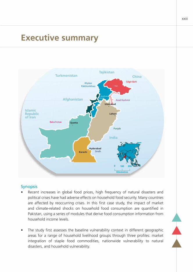
political crises have had adverse effects on household food security. Many countries are affected by reoccurring crises. In this first case study, the impact of market and climate-related shocks on household food consumption are quantified in Pakistan, using a series of modules that derive food consumption information from household income levels.
• The study first assesses the baseline vulnerability context in different geographic areas for a range of household livelihood groups through three profiles: market integration of staple food commodities, nationwide vulnerability to natural disasters, and household vulnerability.
Quetta
Islamabad
Hyderabad
Lahore
Karachi
Islamic Republic of Iran
Afghanistan
TurkmenistanTajikistan
China
India
0 100 200
Kilometres

EXECUTIVE SUMMARYxxiv
• The results of the simulation model indicate that the number of undernourished people (as per the Government of Pakistan’s calorie consumption threshold of 2 350 kcal/adult/day) increased from 77.6 million in 2005/06 to 95.7 million by the end of 2010. The increase can be attributed to price inflation (about 13 million people) and to the massive flood disaster in August 2010 (an additional five million people). The consumption shortfall for the undernourished population equals 6.2 million tonnes of wheat per annum to combat the impacts of the recent shocks.
• If a lower minimum per capita consumption standard of 2 100 kcal/person/day is applied, the number of undernourished people reaches 99.2 million (an additional 11.5 million owing to price inflation and five million because of floods, from a baseline value of 82.7 million). The national food gap becomes some 6 million tonnes of wheat per annum. If the minimum daily energy requirement of 1 730 kcal/person/day is used, the number of undernourished people becomes 65 million (an additional 14 million because of price inflation and 7 million because of floods, from a baseline value of 44 million), and the national food gap becomes 2.7 million tonnes per annum.
• Pakistan’s per capita wheat consumption has been declining in recent years in response to high prices and the reduction in incomes, leading to a rise in wheat stocks. In terms of the national balance sheet, Pakistan is expected to be balanced in wheat while continuing to be a net exporter in rice, albeit with a reduction in volume by over one million tonne.
Background and approachRecently there has been a marked increase in the number of countries facing food crises. Some of the underlying causes have included higher global food commodity price and increased volatility, higher frequency of severe natural disasters and political crises. National and global methods for prompt assessments are weak in supporting timely responses to food crises in many developing countries. While many sudden-onset natural disasters leave little time for assessment and response, man-made disasters present even more challenges to conducting increasingly complex and in-depth analyses. Therefore, there has been an urgent need to develop an effective Early Warning System that signals potential shocks and allows a quick response to crises.
This report presents such a system: a shock impact modeling system (SISMOD) that was developed jointly by WFP and FAO, to simulate the impacts of shocks on household food consumption. The SISMOD builds on existing nationally representative household survey data. This model reduces the need for in-depth nationwide assessments, which can then be limited to the most affected areas and populations. Geographic and community targeting

EXECUTIVE SUMMARY xxv
is made possible as the SISMOD provides estimates of the proportion of undernourished people by livelihood, income group and geographical area. It is being piloted in selected Low- Income Food- Deficit Countries (LIFDCs) that are highly vulnerable to reoccurring crises.1
The results of the Pakistan case study are presented here. In recent years, Pakistan has faced several crises, including the 2008 global food, fuel and financial crises, and a series of major natural disasters, which have increased undernourishment significantly and sent shockwaves through the national economy. In 2008, a UN Interagency mission was conducted in Pakistan in order to assess the impact of food price hikes in the country. This mission was supported by the Government of Pakistan and other stakeholders.2 As the analytical method developed for this assessment was recognized to be very useful, the methodology was further refined, in order to enable effective replication in other countries vulnerable to large-scale shocks.
The project consisted of two parts. In part 1, the vulnerability context of Pakistan was assessed using baseline data (i.e. without shocks), and the areas and livelihood groups most vulnerable to potential shocks were identified. Three profiles were used to assess the vulnerability context. The first provides a market integration analysis of staple food commodities, and determines the markets that are most receptive or vulnerable to international and domestic food price shocks. The second profile reviews the historical records of nationwide vulnerability to natural disasters and highlights the areas that are most vulnerable to climate shocks. An understanding of the relationship between weather patterns and staple crop production, and the implications for household food security are provided. The third profile estimates the baseline caloric intake of households and analyses the vulnerability of livelihood groups to shocks by combining households’ main income sources with the shock factors. These three baseline vulnerability profiles provided contextual information for the modeling by highlighting factors that make households sensitive to market and climate shocks.
The second part was the simulation of the impact of shocks on household food consumption (measured by caloric intake) through a series of modules following three steps: estimation of incomes, allocation of incomes through a two-stage budget allocation demand system by income group, and estimation of equivalent caloric intake. The simulation results show the population groups that were most affected by previous shocks and the groups that are most likely to be affected by future shocks.
1 These countries include: Bangladesh, Tajikistan, Tanzania, Nepal and Pakistan.2 The UN Inter Agency (FAO/UNDP/UNICEF/WFP/WHO) Assessment Mission. High Food Prices in Pakistan:
Impact Assessment and the Way Forward http://www.un.org.pk/wfp/Pakistan_High%20Food%20Prices%20_11%20Aug%202008_.pdf


1. Introduction
1
1.1 Background and rationaleIn recent years, the increase in global food commodity price and their volatility, climate change with higher frequency of severe natural disasters, and political crises have had adverse effects on food security. Both food producing/exporting countries and Low-Income Food-Deficit Countries (LIFDCs) are affected by reoccurring crises, which often send shockwaves through national economies and households, leading to a heightened situation of food insecurity. Estimates show that more than 1 billion people are undernourished worldwide; a substantial increase has occurred in the number of undernourished people in recent years as a result of these shocks (FAO, 2009).
National and global methods for prompt assessments and estimates of the impacts of shocks are weak in supporting timely national responses to food crises in many developing countries. Many sudden-onset natural disasters leave inadequate time for assessment, planning and response. Man-made disasters present even more technical challenges towards conducting increasingly complex and in-depth analyses of socio-economic factors.
In view of the above, a shock impact modeling system (SISMOD) is being developed jointly by the Food Security Analysis Service (OSZA/VAM) of the World Food Programme (WFP) and the Global Information and Early Warning System (GIEWS) of the Food and Agriculture Organization (FAO) to simulate the shock impact on household food consumption. The SISMOD builds on existing nationally representative household survey data. This model is regarded as a strong alternative to nationwide assessments, as it can be used as a cost and time-effective tool by reducing the scope of in-depth ground-truthing assessments to the most affected areas and populations. The results of the simulation can also support early warning for potential shocks and early response to shocks that have taken place. The SISMOD provides estimates of the proportion of undernourished people by livelihood and income groups, as well as by geographical area. Therefore, it can contribute to geographic and community targeting. It is being piloted in selected LIFDCs that are highly vulnerable to reoccurring crises.3
Pakistan is the first of the five case studies. In recent years, Pakistan has been faced with the combined impacts of the 2008 global food price, fuel and financial crises and a series of climate shocks, which have increased undernourishment significantly.
3 These countries are Bangladesh, Burkina Faso, Malawi, Nepal and Pakistan.

Food price volatility and natural hazards in Pakistan2
Pakistan has experienced several natural disasters over the past few years, from the massive Kashmir earthquake in October 2005 to the August 2010 flood, which affected over twenty million people (EM-DAT, 2010). These events have all sent shockwaves through the national economy and aggravated the food insecurity situation especially of vulnerable population.
In 2008, a United Nations Interagency mission was conducted in Pakistan, supported by the Government of Pakistan and other stakeholders, to conduct an assessment of the impacts of food price hikes in the country.4 The findings and recommendations of this assessment resulted in the rapid launch of a safety-net program for vulnerable populations in the most affected areas as well as in policy action within the framework of a National Task Force on Food Security established by the Prime Minister. The analytical method used for the inter-agency assessment was recognized as very useful. As a result, it was recommended that the methodology and tools be refined, in order to ensure effective replication in other countries that are subject to large-scale shocks.
1.2 ApproachThe approach to this project and the present report is two-fold: to assess the vulnerability profile of the country and to develop a shock simulation model. Part one assesses the vulnerability context of Pakistan using baseline data (i.e. without shocks). It identifies the areas and livelihood groups that are most vulnerable to potential shocks and describes the food security situation of households measured in terms of caloric intake. This vulnerability profile provides contextual information for the modeling exercise by highlighting factors that make households sensitive to market and climate shocks.
Part two develops a framework for the Shock Impact Modeling System (SISMOD) which quantifies the impact of the recent market and climate shocks on household food consumption in Pakistan. The simulation results show which population groups are most affected by previous shocks and which groups are most likely to be severely affected by future shocks. Chapter 2 provides a methodological note on the SISMOD and market integration and crop production monitoring analyses.
Part one: Vulnerability profilesThe vulnerability context of Pakistan was assessed through three profiles. The first vulnerability profile, Market Environment and Vulnerability to Food Price Shocks, provides a market integration analysis of staple food commodities, and determines the markets that are most receptive or vulnerable to international and domestic food
4 The UN Inter Agency (FAO/UNDP/UNICEF/WFP/WHO) Assessment Mission. High Food Prices in Pakistan: Impact Assessment and the Way Forward
http://www.un.org.pk/wfp/Pakistan_High%20Food%20Prices%20_11%20Aug%202008_.pdf

Chapter 1. Introduction 3
price shocks. This chapter provides brief contextual information on the macroeconomic context, trends in the agricultural sector, and trade policies, to identify the current trends among shock factors. This profile also provides parameters on price transmission for the SISMOD.
The second profile, Vulnerability to Natural Risks, Shocks and Hazards, reviews the historical records of nationwide vulnerability to natural disasters and highlights the areas that are most vulnerable to climate shocks. It provides an understanding of the relationship between weather patterns and staple crop production and the implications for household food security. This profile provides the parameters for crop production monitoring, taking into account the impacts of weather related variables such as rainfall. The estimated productions are then used in the SISMOD.
The third profile, Household Vulnerability and Food Security, estimates the baseline caloric intake of households and analyses the vulnerability of livelihood groups to shocks by combining households’ main income sources with the shock factors. In this third profile, it is assumed that the extent to which the impact of a shock is transmitted to households largely depends on their main income sources and on their level of dependency on markets.
Part two: Shock impact modeling system (SISMOD): Simulating the impacts of shocks on household food consumptionThe second part, and core of this report, is the simulation of the impact of shocks on household food consumption measured by caloric intake. The simulation model (SISMOD) estimates the impacts of market and climate shocks on household caloric intake through a series of modules following three steps: estimation of incomes, allocation of incomes through a two-stage budget allocation demand system by income groups, and estimation of equivalent caloric intake. The SISMOD simulates the percentage change in households’ caloric intake from the baseline situation, the corresponding number of undernourished people and the food requirements to meet the needs of the affected people. The simulation results show the population groups that were most affected by previous shocks and the groups that are most likely to be affected by future shocks.

2. Methodology
5
The following methodological note provides a detailed description of the approach and methods used in this assessment. This methodology chapter is organized into four main sections. The first section provides the theoretical background of the decision-making process of agricultural households. The second section explains the general framework of the Shock Impact Modeling System (SISMOD), to connect the various components which simulate shock factors on income, expenditures, and consumption. The third section describes the methods used in the market integration analysis and crop production analysis in the vulnerability profiling and in deriving parameters for market and crop monitoring in SISMOD. The fourth section provides an in-depth methodological note on SISMOD, which articulates the process of simulating the impacts of shock factors on household food consumption, by simulating shocks on household income, simulating household income to total/food expenditures, and measuring undernourishment and food needs.
2.1 Theoretical background: How household income and price variations impact food consumption
This study adopts the Agricultural Household Models (AHM) approach developed by Singh et al. (1986). Household-farm models are used to analyse how household-specific transaction costs shape the impacts of exogenous factors, like policy and market changes in rural areas. The application of such modeling techniques have included a gambit of research initiatives, ranging from technology adoption and migration to deforestation and biodiversity. It is now becoming a tool for price policy analysis.
The AHM approach developed by Singh et al. (1986) incorporates both the production and consumption sides, integrates the price effects on different markets, and takes in account the interaction between them. Previous models, like a single-market approach have not captured such a comprehensive effect, which consider consumers and producers separately. Household-farm models acknowledge that production and consumption decisions are linked because the deciding entity (rural household) is both a producer and consumer (Kuroda and Yotopoulos, 1978). An intricate source of the household income is farm profits, which include implicit profits from goods produced and consumed by the same household. Household consumption includes goods that are both purchased from the market and self-produced. As long as perfect markets for all goods, including labour, exist, the household is indifferent between consuming self-produced and market-purchased goods.

Food price volatility and natural hazards in Pakistan6
The fundamental difference between an AHM and pure consumer model is that the household budget is generally assumed to be fixed in a pure consumer model, while in AHM it is endogenous and depends on production decisions that contribute to income through farm profits in AHM. To the standard Slutsky effects of the consumer model, AHM adds an additional, “farm profit” effect, which can be positive or negative. Therefore, the traditional price effect, where household demand decreases as a result of price increases, is comprised by the farm profits effect, which adds a positive influence to the negative Slutsky effects on food demand that may increase household food consumption.
Full income represents the household budget constraint. As a consumer, the household selects a consumption bundle to maximize utility subject to his income, given prices of all consumption goods. Utility-maximizing consumption is expressed in the following form:
(1) C*i = Ci (P, Y*)
In the standard consumer model, consumption of goods (C*i) depends on own prices, prices of related goods (P), and income (Y*). However, in the household-farm model, income is endogenous and depends upon production decisions.
Market equilibrium conditions for individual goods or factors depend upon whether the item or factor in question is tradable or non-tradable for the household. For tradable goods, prices are exogenous, determined by outside markets. Markets clear through supply and demand and determine the marketed surplus (MS*):
(2) MS*i = Q*i - C*i , where Q = Supply, and C = Demand
Use of household-farm models for comparative static analysis for simulationThe motivation for constructing AHM is to understand impacts of polices and other exogenous shocks on household-farm behavior. Following Ulimwengu and Ramadan (2009), the most general form of the comparative static equations in term of own-price shock is the following:
(3)
A change in the price (pi) of a given commodity (i) affects both the supply and the demand decisions. The net impact on household food consumption (qi )depends on the importance of the commodity in terms of both consumption and profit. In equation 3, the first term on the right-hand side of above equation is the direct impact on consumption. The second term on the right-hand side of the above equation is the profit/income effect,
dqi
dpi
=qi
pi
+qi
Ri
Ri
pi
Chapter 2. Methodology 7
which indirectly effects through profit/income (Ri). In other words, the change in price affects the farm profit/income, which in turn affects the full income available for the household. The final impact of the price change on the quantity consumed is a net effect from both terms, which depends on which effect is the most important.
The above equation can be rewritten in term of elasticities as:
(4)
The change of food price is a function of own-price elasticity ( pi ), income elasticity ( R), and profit elasticity ( ).
The equation can be reordered as the following:
(5)
Similarly, the cross price effects of commodity j on the consumed quantity i of commodity I can be derived in the elasticity terms as follows: (6)
Hence, the net impact of food price changes on food consumption of each commodity is a function of own-price elasticity, cross-price elasticities, income elasticity, and profit elasticity with respect to food prices.
In terms of climate shocks, such as droughts or floods, both prices and profit/income may be affected. The price effects can be analysed by partial equilibrium of commodities at market level. The shock impact on income/profit can be assessed by linking household production and profit to the shock factors (the framework is presented in the next section).
The own-price elasticity, cross-price elasticities, and income elasticity will be estimated by a demand system based on household survey data. The details on the data and estimation methods are provided in the following sections.
2.2 Framework of shock impact modeling system (SISMOD): Simulating effects on household food consumption
The shock impact modeling system is composed of several modules that represent the decision-making process of an agricultural household. This process determines the
Food price volatility and natural hazards in Pakistan8
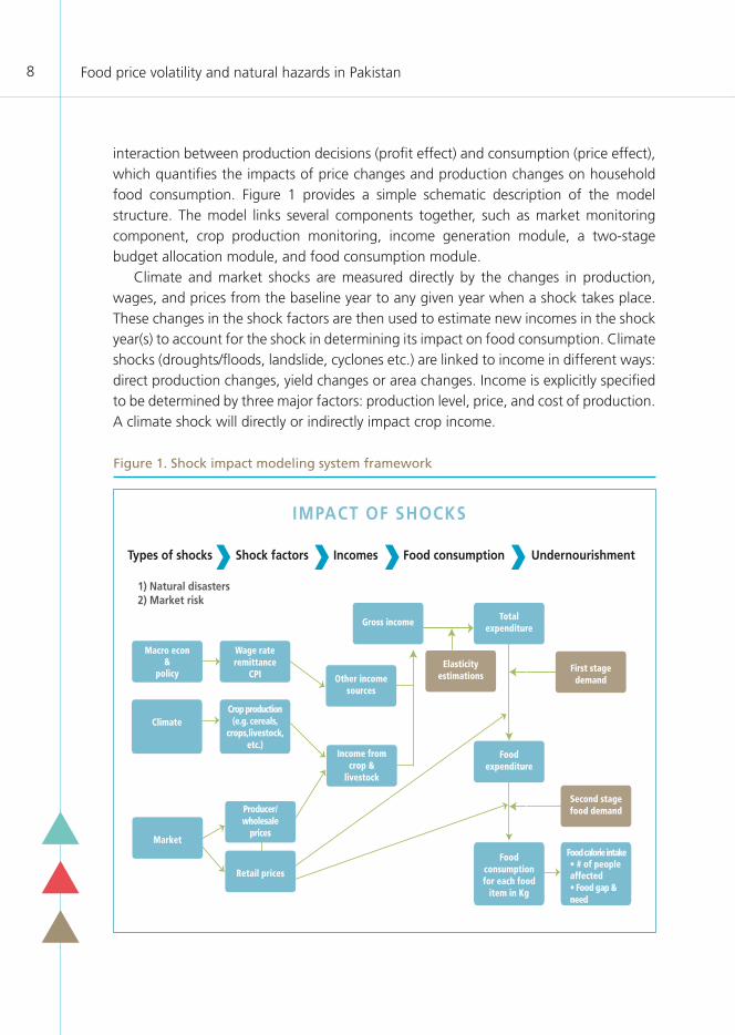
interaction between production decisions (profit effect) and consumption (price effect), which quantifies the impacts of price changes and production changes on household food consumption. Figure 1 provides a simple schematic description of the model structure. The model links several components together, such as market monitoring component, crop production monitoring, income generation module, a two-stage budget allocation module, and food consumption module.
Climate and market shocks are measured directly by the changes in production, wages, and prices from the baseline year to any given year when a shock takes place. These changes in the shock factors are then used to estimate new incomes in the shock year(s) to account for the shock in determining its impact on food consumption. Climate shocks (droughts/floods, landslide, cyclones etc.) are linked to income in different ways: direct production changes, yield changes or area changes. Income is explicitly specified to be determined by three major factors: production level, price, and cost of production. A climate shock will directly or indirectly impact crop income.
Figure 1. Shock impact modeling system framework
IMPACT OF SHOCKS
Types of shocks Shock factors Incomes Food consumption Undernourishment
1) Natural disasters2) Market risk
Wage rateremittance
CPI
Crop production(e.g. cereals,
crops,livestock, etc.)
Gross income
Other incomesources
Totalexpenditure
Foodexpenditure
First stage demand
Second stage food demand
Elasticityestimations
Food consumption for each food
item in Kg
Food calorie intake• # of people affected• Food gap & need
Income fromcrop &
livestock
Retail prices
Producer/wholesale
pricesMarket
Macro econ&
policy
Climate

Chapter 2. Methodology 9
Crop production monitoring and market monitoring are two modules used to track the changes in the shock factors, either based on past patterns for simulating the impact of past shocks for ex-post analysis or based on forecasted changes for ex-ante analysis. For early warning purpose, crop harvested area of a specific crop i (for example, maize) is a function of own price, competing crop prices, total land owned in the household, and household size. Crop production is specified as a area and yield, which is a function of rainfall and time trend, a proxy indicator of technology development.
The market monitoring module includes a commodity partial equilibrium5 model(PE) and a set of price transmission equations. Price formulation, in individual country sub-models, is specified as either price transmission from the world price or market clearing when there are significant restrictions in trade flow. The PE aims to clear the market and generate market prices in the national/regional leading market. Prices in local markets are derived by estimated price transmission elasticities.
The income generation module is used to link shocks to household income, which is aggregated into the following categories: crop income, livestock income, agricultural wage income,6 non-agricultural wage income, public wage income, remittance income, and other income. Each income category is subject to different shocks directly or indirectly. Crop income is categorized by major crop in order to assess the impact of different shocks in different seasons. Crop income is separated into wheat, rice, maize, pulses, cotton, sugarcane, and other crop income. Other income in the households such as wage income is a function of GDP, wage rate, and CPI.
The food consumption module is the core of the system, which simulates the impacts of income and price changes on food consumption. Food consumption impact analyses hinge critically on the underling functional form for representing consumer demand. Simple functional forms can lead to unrealistic estimations by failing to capture changes in income and price elasticities of demand for different population groups. The two-stage budgeting procedure assumes that the consumer’s utility maximization decision can be decomposed into two separate steps. In the first stage, total household expenditure is broken down over eight broad commodity groups which include: food, clothing, fuel, housing, durable goods, education, medical, and other items. In the second stage, household food expenditure is allocated over ten food subgroups which include: rice;
5 In structure of the partial equilibrium models, the following identity is satisfied for each country/region and the world: Beginning Stock + Production + Imports = Ending Stock + Consumption + Exports. Pro-duction is divided into yield and area equations, while consumption is divided into food, feed and other demand. To satisfy the identity, two different methods are used. In most of the countries, domestic price is modeled as a function of the world price with a price transmission equation, and the identity is satisfied with one of the variables set as the residual. In other cases, prices are solved to satisfy the identity
6 The shock model assumes that macroeconomic variables, such as GDP, population (urban/rural), em-ployment and wage rates, and exchange rates, are exogenous variables that are monitored for ex-post analysis or are based on the projections by other studies.
Food price volatility and natural hazards in Pakistan10
wheat; other Cereals; potatoes; meat; fish and eggs; milk products; vegetables and fruits; fats and oils; spices and sugar; and non-alcoholic beverages.
The food consumption in quantity is converted to calorie intake by using a food composition table. Food security indicators related to household undernourishment are then calculated based on daily per capita calorie intake. The major indicators include: mean and distribution (CV) of per capita calorie intake, undernourishment (head count, gap and square of gap), ratio of calorie intake from cereal in total calorie intake (food quality indicator), food gap (in wheat/rice/maize equivalent) for vulnerable groups. Percentage of people who cannot meet a certain requirement dietary energy consumption is measured by several levels of daily caloric intake consumption requirements for food aid/assistance intervention analysis (Smith et al., 2006).
2.3 Methodological note on market and climate shock modules
2.3.1 Market integration and estimates of price transmission elasticitiesThe following methodology is used to measure both the degree of price integration among major commodities to identify the most vulnerable markets to price shocks, and to derive parameters on price transmission for SISMOD. The degree of price transmission between markets reflects the level of market integration. Integrated markets are those where price signals are transferred from one to another, allowing physical arbitrage to adjust any disturbances in these markets; integrated markets are thus a sign of efficiency. Spatial market integration refers to co-movements or the long-run relationship among prices. It is defined as the smooth transmission of price signals and information across spatially separated markets. Two markets are assumed integrated if price changes in one market are manifested in an identical price response in another market (Barret, 1996).
The most common measures of spatial market integration between time series of commodity prices are the bivariate correlation coefficients. However, there are weaknesses associated with the use of price correlation coefficients as measures of market integration: there is the chance that the correlations could be spurious, rather than resulting from the integrated nature of the markets (Barrett, 1996). This analysis recognized these weaknesses and augmented the correlation coefficient approach by co-integration tests and Granger causality tests.
• Co-integration tests:The first step of our analysis consists in determining the order of integration of our variables by using ADF, Phillips Perron and KPSS tests. It is well known that regressing non-stationary time series is likely to give spurious results (Granger and Newbold, 1974). Spurious regression refers to the regression that tends to accept a false relation or reject

Chapter 2. Methodology 11
a true relation by flawing regression schemes. That is the reason why for non-stationary time series it is advisable to work with their differences.
However, regressing first order integrated, i.e. I(1) dependant variables Yt on I(1) independent variables Xt can be informative, but only if these variables are related in a precise sense, i.e., if they are co-integrated. Price co-integration implies that prices move together in the long-run, although in the short run they may drift apart, and this is consistent with the concept of market integration.
If Yt and Xt are two I(1) processes, then, in general, Yt - t is an I(1) process for any number . Nevertheless, it is possible that for some ≠0, Yt - t is a I(0) process. If such a exists, then Y and X are said to be co-integrated. If the data are cointegrated, then we can legitimately estimate a model using the levels of the data to estimate the long-run equilibrating relationship between the variables.
The long-run relationship is given as:
Yt = + t + μt
• Error correction model estimation: If two variables are co-integrated, the following error correction model can be estimated:
yt = t-1 t-1 t-1 yt-1 t
yt and t are the log of two different markets
Δ is the difference operator , and are the estimated parameters, and t is the error term
The term (yt-1- t-1 ) is called the error correction term. If yt-1 > t-1 that means that yt-1
is too high above its equilibrium value, then the negative value of corrects the error. reflects the speed of adjustment: the speed by which prices adjust to their long-run
relationship
Since prices are expressed in logarithms, the coefficient of change in the market t ( ) is the short-run elasticity of the price in the market y relative to the price on the market . It represents the percentage adjustment of price on market y after 1 percent shock in price on market . The co-integration factor ( ) is the long-run elasticity of price transmission of market y in relation to market .

Food price volatility and natural hazards in Pakistan12
The distinction between short-run and long-run price transmission is important as changes in the price at one market may take time to be transmitted to the other markets (due to policies, transportation costs etc.).
• Granger causality tests:If two time-series are cointegrated, then there must be Granger causality between them - either one-way or in both directions. Cointegration tests themselves cannot establish the direction of causality but tests can be applied to cointegrating VARs. Therefore, Granger causality provides additional evidence as to whether, and in which direction, price transmission is occurring between two series.
If past X contains useful information (in addition to the information in past Y) to predict future values of Y, X is said to “Granger causes” Y. Granger causality tests help us to identify the leading markets. A market is considered to be a leading market when past prices significantly contribute to the formation of current prices on other domestic and/or regional markets. There is a possibility of unidirectional causality, bidirectional causality or none. An unidirectional causality may indicate the direction of information flow or of trade, but it is also a sign of information inefficiency (Gupta and Mueller, 1982).
2.3.2 Staple crop production monitoring The following methodological note on crop production monitoring is used both to display the relationship between weather patterns and crop production in the vulnerability profiling, as well as to derive parameters that estimate changes in crop production for application in SISMOD. Traditionally, econometric models for forecasting crop production or crop yield can be characterized as empirical statistical regression equations. These regression equations link regional production or yield with independent “predictor variables”, known as factors. In such models, the dependent variable is the regional production/yield whereas the independent variables can be defined by environmental variables such as weather variables or indices. Predictor variables include the NDVI (Normalized Difference Vegetation Index – satellite index), farm inputs (e.g. fertilizer use), or outputs from simulation models (e.g. average soil moisture).
The main premise behind this forecasting approach, termed as “parametric”, is that the model is derived on the basis of historical production, yield and climatic data through a “calibration” process. The model is then applied to data from a more recent time period by using current crop and within-season data, to produce a production or yield forecast.
The approach taken in this work can be characterized as parametric due to two factors:

Chapter 2. Methodology 13
a) it derives or requires a number of parameters, such as regression coefficients, and these parameters in turn define the crop simulation models;
b) it seeks to pinpoint specific factors commonly associated with crop production/yield and to measure the impact.
In the context of Pakistan, the forecasting process relies on a crop simulation model developed by using regression equations, by rainfall data, NDVI, soil moisture, surface temperature, production and yield dataset for the respective region. This model is contingent on the idea that physical factors (e.g. rainfall, NDVI, surface temperature, and soil moisture) are significant in determining crop production. As with rainfall data, data on NDVI, soil moisture, and surface temperature are used on a temporal annual average basis from July 1974 to June 2010, and be adjusted to account for the crop calendar. For the purpose of this study, we use cumulative monthly rainfall data covering the period July 1974 to June 2010, where precipitation is measured in millimeters.
Crop production data are calculated on an annual basis from 1974 to 2008. Crop production data are measured in metric tonnes and cultivated land area is measured in hectares. It follows that crop yield is calculated by dividing the annual crop production data (in MTs) by the cultivated area (Hectares). To account for the varying climate and geography of Pakistan, we use data gathered at the provincial level, classified according to four of the largest Provinces: Baluchistan, Khyber Pakhtunkhwa (KPK—formerly known as North-West Frontier Province, NWFP), Punjab and Sindh.
This model uses regression coefficients for rainfall and intercept to forecast annual crop production and yield. The rationale for the use of only two parameters in defining our crop simulation model is that the relationship between rainfall and crop production/yield will demonstrate a strong, positive relationship in countries characterized by rain-fed agricultural systems.
Estimation equationThis simple regression describes the nature of the relationship between annual crop production or crop yield, as being dependent on the amount of rainfall. The implicit stipulation of this simple model is that the relationship between these two variables is positive and strong.
(7) y = c1 + a1
where y = crop production or crop yield, a1 = slope of rainfall, RF = cumulative monthly rainfall (July 1974 to June 2010 in millimeters), c1 = regression constant and = error term.

Food price volatility and natural hazards in Pakistan14
Crop production or yield forecasting We substitute the values for the intercept (c1) and the regression coefficient (a1) to estimate the trend crop production or yield. The equation used to forecast trend crop production or yield is as follows:
(8) yt = c1 + a1
where t = trendline, 1974 (first year in the dataset).
It is worth noting that when linking changes in annual crop production or yield to changes in the amount of monthly cumulative rainfall (monthly average or long-run pattern), exogenous factors should be removed from the model.
The output from the forecast equation (10) represents the trend crop production or yield for each year from 1974 to 2010, based on historical trends in the dataset. In turn, this annually estimated trend crop production or yield figure is subsequently used alongside the actual crop production or yield figure to calculate the deviation from the forecast. Hence, the deviation from the forecast is equal to the difference between actual crop production or yield (y) and estimated crop production or yield, based on historical trends in the data (yt ).
Moving forward, the goal is to expand on the earlier regression analysis by incorporating the impact of independent physical factors such as rainfall, NDVI, soil moisture and surface temperature on annual crop production or crop yield in developing countries such that:
(9) y = c1 + a1 RF + a2 NDVI + a3 ST + a4
where y = crop production or crop yield, a1 = slope of rainfall, a2 = slope of the NDVI, a3 = slope of ST, a4 = slope of SM, RF = cumulative monthly rainfall (July 1974 to June 2010 in millimeters), NDVI = Normalized Difference Vegetation Index, ST = Surface Temperature, SM = Soil Moisture, c1 = regression constant and = error term.
Accounting for weather shocks Explaining the linkages between climatic variability and crop production or yield also entails investigating the impact of unexpected weather shocks. For the purpose of this analysis, we specify an annual rainfall threshold which stands as a benchmark against which to compare the effect of a loss in crop production and yield that arises as a consequence of natural disasters. Furthermore, by identifying the particular year and type of natural disaster that occurs in a given country, it would be possible to remove abnormalities in the dataset based on historical

Chapter 2. Methodology 15
trends. These abnormalities would otherwise distort the relationship between crop production/yield and rainfall. These outliers in the rainfall dataset are pinpointed by using a specific threshold to categorize a particular event as a natural disaster. For the purposes of this study, the types of natural disaster that are of particular concern are droughts and flooding.
The XY scatter plots shown in this report were produced with both the regression line and regression equations. The strength of the relationship between cumulative rainfall and annual wheat production is represented by the correlation coefficient, the R² value. For Pakistan, the predictive power of the relationship is higher for the cumulative rainfall.
2.4 Pass-through of shocks: The income generation moduleAs mentioned above, the market monitoring and crop production monitoring modules are used to derive the changes in the shocks factors (production, prices, wages) from the baseline year (without shock) to any given year when a shock takes place. These two modules track the changes in shocks factors either based on past patterns for stimulating the impacts of past shocks for ex-post analysis, or based on forecasted changes for ex-ante analysis. Production changes are estimated by field missions (ex-post) or forecast based on rainfall/temperature (ex-ante). Producer price of output is based on the real price changes (ex-post) or forecast based on the partial equilibrium or/and price transmission (ex-ante). Therefore, the income generation module estimates new incomes in the shock year(s) based on the changes in the shock factors to account for the shock in determining its impact on food consumption.
2.4.1 Components of aggregate incomeHousehold income sources are disaggregated by the following components:
Crop income: The estimation of crop income accounts for the sale of crop production, crop by-product production, sharecropping, the consumption of household crop production, net of all expenditures incurred in realizing these activities, such as agricultural inputs (seeds, pesticides and fertilizers) and the hiring of farm labour.
Livestock income: The livestock income category includes income from the sale and barter of livestock, livestock by-product production (i.e. milk, eggs, honey etc.), net of expenses related to livestock production (e.g. fodder, medicines) and livestock purchases, plus the value of household consumption of own livestock and livestock by-product production. The values of own consumption are estimates based on the food consumption/expenditure section of the questionnaire. In cases where this information is not available in that module, the consumption amount is obtained from

Food price volatility and natural hazards in Pakistan16
the agricultural module. The approach for valuation of own consumption is the same as for the valuation of crop own-consumption.
Wage income: Wage income consists of all income received in the form of employee compensation either in cash or in kind. Wage employment income is first disaggregated by industry in the survey. The classification is based on the UN International Standards Industrial Classification of all Economic Activities (ISIC). As the classification of industries changes over time, the most appropriate revision of the ISIC classification standards is chosen based on the year the survey was undertaken. In the survey, industries are grouped into ten principal categories: agriculture; forestry and fishing; mining; manufacturing; utilities; construction; commerce; transportation, communications and storage; finance and real estate; services; and miscellaneous. Using this industrial classification, total wage employment income is separated into three aggregate categories: agricultural wages, non-agricultural private wages, and non-agricultural public wages.
Remittance income: Given the increasing importance of remittance income in food security for poor households, remittance income is separated from other income. Remittance income can be sourced by domestic transfer income and overseas transfer income.
Summary tables of the percentage income by each category and the share of each crop in total crop income are presented in Appendix 1 (see Table A1.1). In Pakistan, crop income constitutes the largest part of income for rural agriculturalists. The crop income in Pakistan is disaggregated into wheat, rice, maize, cotton, sugarcane, pulse, and fruits.
2.4.2 Net income of total crop production Since the survey did not report input and cost of production of individual crops, the net income of crop production is estimated at the aggregated level: net income of total crop production = sum of gross crop income – total cost of crop production.
Crop area harvested for a specific crop (for example: wheat, rice, maize) is a function of own price (Pio ), competing crop prices (Pic ), total land owned in the household (Land j ), and household size.
(10) Aij = f (Pio, Pic, Land j, Househols Size j )
Crop yield is specified as a function of rainfall or the Normalized Difference Vegetation Index, and time trend (representing the technology development), expressed as:
(11) y1 =f
NVPI
raintime

Chapter 2. Methodology 17
Wage income is a function of wage rate, GDP, and CPI and expressed as:
(12)
Total income is expressed as:
(13)
2.5 From income estimates to total and food expendituresThe ‘average propensity to consume’ or APC is defined as the ratio of a household’s spending or consumption to its disposable income. In turn, the ‘average propensity to save’ or APS is the ratio of the family’s savings to its disposable income. The resulting sum of APC and APS is one; that is, one hundred percent of disposable income.
To pass the shocks to income and then to total household expenditure, the household APC was estimated for urban and rural populations in Pakistan by using Pakistan Social and Living Standards Measurement Survey (PSLM) data. The equation for total expenditure is specified as a function of household income, controlling for households social and demographic characteristics such as household size, location, and gender of household head, age of household head, and education of household head.
(14)
The elasticities derived are used for the shock model simulation.
Income group separationDifferences in income and household characteristics lead to different household behavior in the acquisition of goods. Food expenditures are almost completely explained by income levels for low income households, while for high income households food expenditures depend on other factors such as household demographic characteristics. The method for classifying households into income groups was based on an analysis of homogeneity of variances of residuals. Following Jensen and Manrique (1996), the procedure has two basic steps, estimation of Engel relations and tests for homoscedasticity of variances. Successive Goldfeld-Quandt tests using the residuals from the Engel estimation were performed in order to classify the household observations into groups with different variances. Classification of households into income groups was determined by setting income boundaries for groups of residuals. The idea is to test whether the variance of the disturbances of one part of the sample is the same as another part (homoscedasticity).
Iio = f(GDP,Wage Rate,CPI)
Ii = PioAiyi
i=1
K
+Iio

Food price volatility and natural hazards in Pakistan18
To do so, first the observations were ordered based on income level (or total food expenditure level) and equally separated in the number of groups desired (i, normally five groups); second, equally separate the sub-observations into three groups (j) within the group (i) and re-estimate independently for each sub-group of observations (j) based on the Engel estimation; third, test whether the variances of the three sub-groups are the same based on the estimation in step two and F-test. If the F-test indicates they are not in the same income group, those observations are moved to the next group i; forth, final income boundaries are determined by repeating the Goldfeld-Quandt tests. In the context of Pakistan, three income groups (low, middle and high) were identified.
2.5.1 First stage demand system (linear expenditure system): Total household expenditure
In this analysis, the first stage allocates total household expenditure to eight broad groups of goods: food, clothing, fuel, housing, durable goods, education, medical items, and other items. A non-Linear Seemingly Unrelated Regression was used to estimate a linear expenditure system (LES) of seven equations for the first-stage budget allocation (Box 1). The advantage of the LES is that it is simple and provides an intuitive economic interpretation, despite its strong separability assumption. The separability assumption is not overly restrictive for such commodities as food, housing, or clothing (Timmer and Aldermand, 1979).
In the LES, demand equations are assumed to be linear in all prices and incomes and the set
of demand functions is expressed in expenditure form:
(1)
with =1 and Y>X . Where P X (P and X are aggregated price and quantity
indices for commodities within group I) is expenditure, and R and are parameters. Y is
household total expenditure. The uncompensated own-price and cross-price elasticities
associated with equation (1) are:
(2) II = (1- I) PJRJ/(PIXI)-1 and
(3) IJ = - I (PJRJ)/(PIXI).
The expenditure elasticities are: (4) μ Y/(P X ).
Box 1. Linear expenditure system (LES) demand equations
PI XI = PI RI + I Y PI
j
RI

Chapter 2. Methodology 19
This study uses Pakistan Social and Living Standards Measurement Survey (PSLM) data of 2001/02, 2003/05, 2005/06, and 2007/08 which recorded all major economic activities in the survey year. Unlike aggregate time series, which are often not conducive to precise estimation of cross-price effects largely due to collinearity of prices, cross-sectional data offer an important advantage in deriving better elasticity estimates. Detailed demographic characteristics collected in cross sectional surveys allow accommodation of heterogeneous preferences, and the typically large sample also provides the degrees of freedom required to estimate a large and disaggregate demand system.
The sample contains variables on rural and urban household income, expenditure, production and consumption, as well as their demographic characteristics. The data used are the panel data of cross sector (by province and income group) and time series (four time periods). The data are derived from aggregated data from the Pakistan National Statistical Office. The aggregated prices for the grouped goods in the first stage are derived based on the Pakistan CPI database and are computed using the Stone aggregation with their expenditure shares as weights in each group.
Results of parameter estimates and elasticities The estimation results for the first-stage demand for eight broad consumption groups are presented in Table 1. All parameters, from the regressions for each income group and entire sample, have the expected signs and appropriate magnitudes. Most parameters are significant at the 1 percent level.
The adjusted R-square is 0.93 for food expenditures for urban and 0.95 for rural, and are greater than 0.8 for all other expenditure groups in both urban and rural.
Table 1: Household demand in Pakistan: Estimated own price elasticities and
expenditure elasticities by rural/urban for the first stage demand system, 2001-2007
Source: Estimated by Joint FAO/WFP Household Modeling Project based on Pakistan HIES data 2005/06. “Food” corresponds to “Food, beverages and tobacco”.
Food Clothing Fuel Housing Durables Medical Education
RURAL PARAMETERS
Own price elasticities
-0.836 -0.820 -0.816 -1.003 -0.878 -0.856 -1.183
Expenditure elasticities
0.874 1.025 1.015 1.295 1.103 1.097 1.562
URBAN PARAMETERS
Own price elasticities
-0.788 -0.797 -0.811 -1.159 -0.961 -0.801 -1.142
Expenditure elasticities
0.792 0.932 0.943 1.429 1.139 0.947 1.377

Food price volatility and natural hazards in Pakistan20
Using the estimated coefficients, uncompensated price and expenditure elasticities are evaluated at the sample means. Own-price elasticity for food is -0.836 in rural and -0.788 in urban. Own-price elasticities for clothing, fuel, medical, and other group are similar to that of food group, ranging from -0.82 to -0.88 in rural and ranging from -0.80 to -0.96 in urban. Relatively, housing and education have more elasticity, with own-price elasticities greater than unity in both rural and urban areas.
Expenditure elasticity for food is 0.87 in rural and 0.79 in urban, the lowest in the broad consumption groups. Education and housing have the highest expenditure elasticities: 1.56 for education and 1.30 for housing in rural and 1.38 for education and 1.43 for housing in urban. These results indicate that the demand for food is less elastic than the demand for the other 6 groups with respect to expenditures. This implies that people would reduce expenditures much more on education and housing during a price shock than on food.
2.5.2 Second stage of food demand systemThe synthetic food demand equation for each food item is defined in per-capita terms and is a function of real price of the commodity, real consumer expenditures per capita and real prices of other foods:
(15)
The real price of the commodity is expected to be negatively related to food demand. The signs of the other two variables are ambiguous because expenditure elasticities can be positive or negative, and other foods can be substitutes or complements.
Given the income and price elasticities, the percentage change in each food item consumed will be determined by percentage of change in price (own and cross price) and percentage of change in income.
The framework of the second stage is summarized in Figure 2.In this second stage, a Linear Almost Ideal Demand System (LAIDS) (Deaton and
Muellbauer 1980) (see Box 2) was estimated for 13 food products: milk and milk products; meat and fish; fruits; potatoes; vegetables; tobacco; sugar; beverage and drinks; wheat; rice; other cereals; edible oils/fats; and spices. A censored linear almost ideal demand system is estimated with a Bayesian Markov chain Monte Carlo procedure (detailed can be found from Kasteridis, Yen, and Fang). The second stage estimates used the household level 2005/06 PSLM data of 15 400 households. Conducted by Pakistan’s Federal Bureau of Statistics, The PSLM is one of the main mechanisms for monitoring the implementation of the Poverty Reduction Strategy Paper of the Government of Pakistan (2003).
Of the 13 equations estimated, statistical significance of demographic variables are most notable in the tobacco equation, with 14 of the 15 variables significant at
),,( PjPfd ii

Chapter 2. Methodology 21
Figure 2. Second stage of food demand system: Deriving food consumption
Food consumption shock model based on food demand system
Computation of expenditure and price elasticity for 13 food groups
Set of synthetic equations for shocks
Grouping of households by per capita total expenditure
Estimation of complete demand system in the second stage by income group
Demographic characteristics
Consider the Linear Almost Ideal Demand System (LAIDS) with L equations for latent share of
each food group in total consumption ( ) for household (Deaton and Muellbauer 1980):
(1)
where are demographic variables, is total expenditure, and is
the price index. The adding-up, homogeneity, and symmetry restrictions are in Equations
(23), (24) and (2), respectively:
(3)
(4)
(5)
Box 2. Model specification

Food price volatility and natural hazards in Pakistan22
the 10 percent significance level or lower, followed by sugar, wheat, and cereals (with nine variables significant), down to rice (three variables significant), and beverages (two variables significant). Of the 78 quadratic price coefficients ( ), over two-thirds (56 coefficients) are significant at the 10 percent level or lower. All but two (meat, fruits) of the coefficients of the expenditure variable ( ), and all the error standard deviations, are significant at the 1 percent level. Over two thirds (or 46) of the 66 error correlation coefficients ( ) are significant at the 10 percent level or lower.
The estimated compensated price and expenditure elasticities are summarized in Tables 2, 3 and 4. The own-price elasticities of beverages are slightly above unity for low, middle and high income groups. In addition, the own-price elasticities are above one for fruits and tobacco in the low income group; for meat in the middle income group, and for rice and oils in the high income group. All other own-price elasticities are below unity, suggesting that demand for food is predominantly inelastic in Pakistan. All expenditure elasticities are positive and significant at the 1 percent level. The largest expenditure elasticities are observed for milk (1.5), fruits (1.0), wheat (1.6) and rice (1.3) in low income groups; for tobacco (1.3) and fruits (1.1) in middle income groups, and for meat (1.0), fruits (1.1) and tobacco (1.3) in high income groups.
The cross-price elasticities show a mix of gross complements and substitutes. Wheat and rice are complements for low income groups while they are substitutes for middle and high income groups. Milk and oils are substitutes to cereals (rice, wheat) in all three income groups. However meat is a complement for wheat in low income groups. Sugar is a substitute to cereals in low and middle income groups.
2.6 Measuring undernourishment and food security indicators
2.6.1 Deriving per capita dietary energy consumption The dietary energy consumption per person is the amount of food, in kilocalorie (kcal)7 per day, for each individual in the total population (FAO, 2008). Food consumption in quantities is converted into dietary energy consumption (DEC) by using energy conversion factors for energy-yielding macronutrients (proteins, fats and carbohydrates). These energy conversion factors for Pakistan were extracted from the conversion factors in Nepal and Bangladesh, as well as by consultation with Pakistan.
Following the FAO method (FAO, 2010), the total dietary energy consumed by individuals depends on the quantity of food consumed and its caloric content:
7 One kcal equals 1 000 calories and one kj equals 1 000 joules. In the International System of Units (ISU), the universal unit of dietary energy is the joule (J). One kcal = 4.184 kJ. The dietary protein consump-tion per person is the amount of protein in food, in grams per day, for each individual in the total population. The dietary fat consumption per person is the amount of fat in food, in grams per day, for each individual in the total population (Data source: FAO Statistics Division).

Chapter 2. Methodology 23
Pric
e el
asti
citi
esEx
pend
itur
e
Milk
Mea
t Fr
uits
Pota
toes
Veg.
Toba
cco
Suga
rBe
v.W
heat
Rice
Cere
als
Oils
Spice
s
Milk
–0.7
93**
*0.
138*
**0.
066*
**0.
025*
**0.
071*
**0.
011*
**0.
107*
**0.
036*
**0.
118*
**0.
055*
**0.
081*
**0.
035*
**0.
051*
**1.
529*
**
Mea
t0.
205*
**–0
.082
***
0.03
8***
–0.0
30**
*–0
.010
–0.0
100.
009
0.00
2–0
.231
***
0.01
70.
053*
**0.
044*
**–0
.004
0.89
1***
Fru
its
0.21
7***
0.08
5***
–1.0
15**
*0.
073*
**0.
055*
**0.
024*
**0.
064*
**–0
.028
***
0.08
4***
0.12
9***
0.09
2***
0.17
9***
0.04
1***
1.02
3***
Pota
-to
es0.
124*
**–0
.091
***
0.10
0***
–0.2
95**
*0.
078*
**0.
046*
**0.
048*
**0.
044*
**–0
.226
***
–0.0
89**
*0.
013
0.22
8***
0.02
0.72
1***
Veg
.0.
176*
**–0
.018
0.03
7***
0.04
0***
–0.5
01**
*0.
034*
**0.
031*
**0.
031*
**–0
.039
0.00
90.
042*
**0.
134*
**0.
025*
*0.
769*
**
Tob
ac-
co0.
215*
**0.
016
0.11
5***
0.13
7***
0.21
1***
–2.3
14**
*0.
034
0.11
8***
0.52
1***
0.36
6***
0.05
1**
0.41
5***
0.11
7***
0.66
3***
Sug
ar0.
184*
**0.
002
0.02
8***
0.01
6***
0.02
0**
–0.0
09*
–0.6
22**
*0.
085*
**0.
109*
**0.
015*
0.02
3***
0.13
9***
0.01
0*0.
584*
**
Bev
.0.
150*
**0.
003
–0.0
40**
*0.
040*
**0.
053*
**0.
031*
**0.
202*
**–1
.404
***
0.54
8***
0.12
4***
0.04
1***
0.21
4***
0.03
8***
0.69
6***
Wh
eat
0.14
3***
–0.1
89**
*0.
026*
*–0
.065
***
–0.0
27*
0.05
2***
0.07
8***
0.17
0***
–0.2
10**
*–0
.061
***
–0.0
54**
*0.
124*
**0.
012
1.57
4***
Ric
e0.
250*
**0.
058*
0.17
5***
–0.0
81**
*0.
021
0.13
9***
0.04
9**
0.13
7***
–0.1
88**
*–0
.831
***
0.02
9*0.
126*
**0.
116*
**1.
256*
**
Cer
eals
0.31
2***
0.13
4***
0.11
0***
0.01
20.
072*
**0.
006
0.06
0***
0.04
2***
–0.1
49**
*0.
024*
–0.7
54**
*0.
101*
**0.
030*
**0.
759*
**
Oils
0.06
4***
0.03
8***
0.08
7***
0.08
2***
0.09
2***
0.05
0***
0.13
3***
0.08
7***
0.16
6***
0.04
4***
0.03
9***
–0.9
66**
*0.
085*
**0.
612*
**
Spic
es0.
201*
**-0
.017
0.04
5***
0.01
70.
041*
*0.
029*
*0.
027*
0.03
6***
0.04
80.
104*
**0.
029*
**0.
207*
**-0
.767
***
0.54
2***
Tab
le 2
: Lo
w in
com
e g
rou
p in
Pak
ista
n: C
om
pen
sate
d p
rice
ela
stic
itie
s an
d in
com
e el
asti
citi
es
Not
e: A
ster
isks
indi
cate
leve
ls o
f st
atis
tical
sig
nific
ance
: ***
1%
; **
5%; *
10%
.So
urce
: Est
imat
ed b
y Jo
int
FAO
/WFP
Hou
seho
ld M
odel
ing
Proj
ect
base
d on
Pak
ista
n H
IES
data
200
5/06
.

Food price volatility and natural hazards in Pakistan24
Pric
e el
asti
citi
esEx
pend
itur
e
Milk
Mea
t Fr
uits
Pota
toes
Veg.
Toba
cco
Suga
rBe
v.W
heat
Rice
Cere
als
Oils
Spice
s
Milk
–0.6
86**
*0.
152*
**–0
.069
***
0.05
6***
0.03
6***
0.17
7***
0.04
1***
0.03
7***
0.11
1***
0.06
0**
0.01
9**
0.05
0***
0.01
7***
0.82
8***
Mea
t0.
302*
**–1
.128
***
0.04
80.
090*
*0.
007
–0.0
950.
053*
**0.
024
0.61
5***
0.10
9–0
.045
*0.
029
–0.0
09**
0.93
0***
Fru
its
–0.1
15**
*0.
022
0.09
0**
0.04
7***
0.03
6***
0.06
2–0
.022
***
0.00
5–0
.136
***
–0.0
030.
017*
–0.0
03–0
.001
1.08
9***
Pota
toes
0.28
8***
0.23
2**
0.15
6***
–0.9
30**
*0.
166*
*0.
097
0.04
60.
02–0
.079
–0.0
56–0
.042
0.12
9**
–0.0
28**
*0.
783*
**
Veg
.0.
156*
**0.
018
0.15
2***
0.18
2**
–0.9
54**
*0.
149*
0.03
1–0
.016
0.09
70.
017
0.05
40.
093
0.01
9*0.
849*
**
Tob
acco
0.16
6***
–0.0
47**
0.03
8**
0.00
8–0
.001
–0.0
17–0
.046
***
–0.0
06–0
.066
**0.
026
–0.0
03–0
.039
***
–0.0
13**
*1.
341*
**
Sug
ar0.
168*
**0.
168*
*–0
.082
***
0.03
20.
023
–0.2
36**
*–0
.724
***
0.18
6***
0.37
5***
0.21
6***
–0.0
37–0
.081
*–0
.008
0.87
9***
Bev
.0.
223*
**0.
083
0.05
60.
017
–0.0
140.
101
0.16
6***
–1.2
91**
*0.
331*
*0.
122
0.00
70.
167*
**0.
031*
**0.
867*
**
Wh
eat
0.13
8***
0.44
4***
–0.1
25**
*–0
.027
0.03
7–0
.195
***
0.09
6***
0.07
9**
–0.8
20**
*0.
210*
**0.
053*
*0.
066*
*0.
045*
**0.
714*
**
Ric
e0.
125*
*0.
110*
0.00
6–0
.015
0.01
80.
035
0.06
9***
0.03
9*0.
281*
**–0
.759
***
0.03
9*0.
034
0.01
6***
0.82
8***
Cer
eals
0.09
9*–0
.149
*0.
087*
*–0
.067
0.07
0.05
1–0
.012
0.00
80.
233*
0.12
7–0
.536
***
0.08
5**
0.00
40.
833*
**
Oils
0.19
9***
0.06
70.
007
0.13
0*0.
089
–0.1
64**
–0.0
450.
143*
**0.
178
0.04
50.
063*
–0.7
09**
*–0
.004
0.80
5***
Spic
es0.
273*
**–0
.169
***
0.01
1–0
.225
***
0.08
2–0
.239
***
–0.0
140.
125*
**0.
727*
**0.
141*
**–0
.007
–0.0
32–0
.673
***
0.66
4***
Tab
le 3
: Mid
dle
inco
me
gro
up
in P
akis
tan
: Co
mp
ensa
ted
pri
ce e
last
icit
ies
and
inco
me
elas
tici
ties
Not
e: A
ster
isks
indi
cate
leve
ls o
f st
atis
tical
sig
nific
ance
: ***
1%
; **
5%; *
10%
.So
urce
: Est
imat
ed b
y Jo
int
FAO
/WFP
Hou
seho
ld M
odel
ing
Proj
ect
base
d on
Pak
ista
n H
IES
data
200
5/06
.

Chapter 2. Methodology 25
Price
ela
stic
itie
sEx
pend
iture
Milk
Mea
t Fr
uits
Pota
toes
Veg.
Toba
cco
Suga
rBe
v.W
heat
Rice
Cere
als
Oils
Spic
es
Milk
–0.8
76**
*0.
025
–0.0
90**
*0.
025*
*–0
.001
–0.0
84**
*0.
022*
**0.
008
0.02
0.01
3–0
.004
0.00
3–0
.002
0.94
1***
Mea
t0.
029
–0.8
73**
*–0
.085
***
0.02
9–0
.031
**–0
.251
***
0.01
10.
014
0.18
5***
0.01
5–0
.027
–0.0
25–0
.010
**1.
017*
**
Fru
its
–0.1
42**
*–0
.078
***
–0.2
78**
*0.
007
–0.0
32**
*–0
.243
***
–0.0
38**
*–0
.007
–0.1
84**
*0.
007
–0.0
04–0
.046
***
–0.0
14**
*1.
052*
**
Pota
toes
0.09
4**
0.07
80.
034
–0.7
99**
*–0
.035
–0.1
17**
0.04
40.
144*
**–0
.336
***
0.06
1–0
.029
0.04
9–0
.017
0.82
8***
Veg
.–0
.003
–0.0
84*
–0.0
99**
*–0
.077
–0.4
23**
*–0
.250
***
0.01
9–0
.043
0.10
4–0
.067
–0.0
170.
013
–0.0
120.
938*
**
Tob
acco
–0.0
93**
*–0
.149
***
–0.1
49**
*–0
.032
***
–0.0
60**
*–0
.245
***
–0.0
81**
*–0
.039
***
–0.2
04**
*–0
.078
***
–0.0
33**
*–0
.086
***
–0.0
26**
*1.
273*
**
Sug
ar0.
071*
**0.
04–0
.073
***
0.02
90.
007
–0.1
94**
*–0
.833
***
0.01
3–0
.093
0.06
8–0
.052
***
0.03
20.
036*
**0.
949*
**
Bev
.0.
044
0.06
70.
004
0.19
6***
–0.0
24–0
.151
***
0.03
7–1
.257
***
0.26
9***
–0.0
60–0
.012
0.04
60.
017
0.82
4***
Wh
eat
0.03
60.
178*
**–0
.172
***
–0.1
30**
*0.
033*
*–0
.266
***
–0.0
130.
075*
**–0
.865
***
0.15
6***
0.02
50.
129*
**0.
004
0.81
0***
Ric
e0.
030.
025
0.03
30.
035
–0.0
21–0
.160
***
0.03
7*–0
.022
0.21
0***
–1.1
88**
*0.
022
0.03
0.00
30.
967*
**
Cer
eals
–0.0
42–0
.079
0–0
.054
–0.0
16–0
.152
***
–0.0
75**
–0.0
210.
071
0.05
7–0
.611
***
0.02
3–0
.029
***
0.92
8***
Oils
0.00
2–0
.032
–0.1
14**
*0.
044
0.01
4–0
.279
***
0.05
1*0.
030.
358*
**0.
062
0.02
–1.0
05**
*0.
013
0.83
7***
Spic
es–0
.022
–0.0
34–0
.095
***
–0.0
79–0
.015
–0.2
29**
*0.
166*
**0.
045
0.01
50.
032
–0.0
68**
*0.
052
–0.5
48**
*0.
780*
**
Tab
le 4
: Hig
h in
com
e g
rou
p in
Pak
ista
n: C
om
pen
sate
d p
rice
ela
stic
itie
s an
d in
com
e el
asti
citi
es
Ast
eris
ks in
dica
te le
vels
of
stat
istic
al s
igni
fican
ce: *
** 1
%; *
* 5%
; * 1
0%.
Sour
ce: E
stim
ated
by
Join
t FA
O/W
FP H
ouse
hold
Mod
elin
g Pr
ojec
t ba
sed
on P
akis
tan
HIE
S da
ta 2
005/
06.

Food price volatility and natural hazards in Pakistan26
(16) Dietary Energy Consumption:
Food consumption is usually measured at the household level, so we define xj as the per-capita quantity of food j, cj is the energy content of food j, and TC the total dietary energy intake, measured in kilocalories per capita. As the energy conversion factors are fixed and they depend on the energy contents of the various macronutrients), the changes in dietary energy consumption are given by the changes in food consumption.
2.6.2 Undernourishment and percentage of people consuming less than the DECR in total population Undernourishment refers to the condition of people whose DEC is continuously below a minimum dietary energy requirement for maintaining a healthy life and carrying out light physical activity. In a specified age and sex group, the minimum energy requirement is the amount of dietary energy per person adequate to meet the energy needs for minimum acceptable weight for attained-height maintaining a healthy life and carrying out a light physical activity. For a population, the minimum energy requirement is the weighted average of the minimum energy requirements of the different age groups (male and female) in the population. Percentage of people consuming less than the DECR is defined as the proportion of the population in a condition of undernourishment. This study measures the prevalence of undernourishment as the percentage of people with daily kilocalorie (kcal) intake <2 350 kcal in adult equivalent (the recommended daily caloric intake for an adult) (Smith et al., 2006). However, other definitions for undernourishment such as 2 100 kcal/day and 1 730 kcal/day were also applied to all categories of the simulation results (Appendices 2 and 3).
The following indices capture different aspects of hunger, presenting a comprehensive picture. The Headcount simply counts the number of the undernourished. The Hunger Gap contains a measure of the Depth of Hunger. The Severity of Hunger captures the degree of inequality among the undernourished. Only joint consideration of these three indices can give an adequate description of undernourishment.
The calculation of undernourishment indices computes the hunger value for each individual and then aggregates these values to obtain an index for all the population. Formulas are as follows:

Chapter 2. Methodology 27
H0i = h0 wi( ) =1 if wi < z
0 if wi zHC =
1
Nh0 wi( )
i=1
N
H1i = h1 wi( ) =z wi
z if wi < z
0 if wi z
HG =1
Nh1 wi( )
i=1
N
H2i = h2 wi( ) =z wi
z
2
if wi < z
0 if wi z
SH =1
Nh2 wi( )
i=1
N
wi
Headcount (HC):
Hunger Gap (HG):
Severity of Hunger (SH):
Where z is the value of the undernourished line, is the per adult equivalent consumption expenditure of the individual i, and N is the total population. For all the indices, when the individual values are summed up they are multiplied by the household size and properly weighted to represent the whole population.
2.6.3 Food gap in quantity of wheat equivalent For a rapid food security assessment, one important indicator is the calculation of the food assistance needed. Food Gap (FG) in quantity of grain (such as wheat) equivalent is calculated for households with DEC below the requirement. The formula for Pakistan is the following:
(19) Food Gap in grain per household = (kcal consumed or available per capita – requirement) x HH size /conversion factor from kcal to kg of grain).
In conclusion, the methodological approach presented above provides two main intermediary outputs that can be used for early warning: the market price transmission effects and the production forecast. In addition, the SISMOD provides important outputs to the understanding of undernourishment status after a shock or in anticipation of a shock:
• the hunger head-count of the undernourishment, i.e. the percentage of undernourished population affected by a shock. This estimate can be presented by gender, geographic setting, income groups or livelihood groups;
• the hunger-gap and the severity of hunger can also be categorized by the different groups mentioned above;
• the food gap in cereal equivalent quantity.


29
3. Economic environment and vulnerability to food price shocks
The following chapter provides a summary of the current economic context in Pakistan and identifies the transmission channels of market shocks in the country. The first part of this chapter provides contextual information on the economic environment in Pakistan by reviewing the macroeconomic context, trade policies and regulations, and the characteristics of the agricultural sector. The core of this chapter provides a market integration analysis and price transmission analysis in Pakistan to determine the degree of wheat, IRRI rice, and basmati rice price transmission between domestic and international markets. The results highlight the markets that are most vulnerable to domestic and international price shocks.
3.1 Macroeconomic context The global food, fuel, and financial crises in 2008 triggered the beginning of an economic slowdown that sent shockwaves around the world. The current global economic deceleration is the result of a variety of simultaneous bubbles or crises, which displayed the interconnection and undrawn boundaries between international and domestic markets. The shockwaves have resulted in tremendous economic challenges which have rippled through national to household economies.
Today, Pakistan’s economy continues to face the combined residual effects of the global financial crisis, the food and fuel crises, the aftermath of various natural disasters, and the continuing volatile security situation. Prior to the 2008 fiscal year Pakistan was the 26th largest economy in the world in terms of purchasing power, and in 2005 Pakistan was the third fastest growing economy in Asia. During the five years prior to 2008, Pakistan’s economy more than doubled in size with an annual GDP growth rate averaging nearly 7 percent. Pakistan, classified as a lower middle income country by the World Bank, had a 2009 GDP valued around USD166 billion using the official exchange rate. However, the economy has experienced a slowdown in growth. As a consequence of the effects of the above mentioned shocks, key macroeconomic indicators are signifying a weakened and unstable economy compared with previous years.
The nominal GDP growth rate dropped from 7.7 percent in 2005 to 2.0 percent in 2008 and 3.7 percent in 2009. In real terms, the GDP growth rate was estimated to be 2.7 percent in 2009 (World Bank, 2011). The largest contributor to Pakistan’s national income is the state supported services sector (especially in transport,
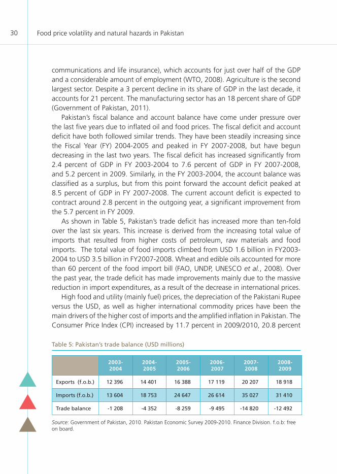
Food price volatility and natural hazards in Pakistan30
communications and life insurance), which accounts for just over half of the GDP and a considerable amount of employment (WTO, 2008). Agriculture is the second largest sector. Despite a 3 percent decline in its share of GDP in the last decade, it accounts for 21 percent. The manufacturing sector has an 18 percent share of GDP (Government of Pakistan, 2011).
Pakistan’s fiscal balance and account balance have come under pressure over the last five years due to inflated oil and food prices. The fiscal deficit and account deficit have both followed similar trends. They have been steadily increasing since the Fiscal Year (FY) 2004-2005 and peaked in FY 2007-2008, but have begun decreasing in the last two years. The fiscal deficit has increased significantly from 2.4 percent of GDP in FY 2003-2004 to 7.6 percent of GDP in FY 2007-2008, and 5.2 percent in 2009. Similarly, in the FY 2003-2004, the account balance was classified as a surplus, but from this point forward the account deficit peaked at 8.5 percent of GDP in FY 2007-2008. The current account deficit is expected to contract around 2.8 percent in the outgoing year, a significant improvement from the 5.7 percent in FY 2009.
As shown in Table 5, Pakistan’s trade deficit has increased more than ten-fold over the last six years. This increase is derived from the increasing total value of imports that resulted from higher costs of petroleum, raw materials and food imports. The total value of food imports climbed from USD 1.6 billion in FY2003-2004 to USD 3.5 billion in FY2007-2008. Wheat and edible oils accounted for more than 60 percent of the food import bill (FAO, UNDP, UNESCO et al., 2008). Over the past year, the trade deficit has made improvements mainly due to the massive reduction in import expenditures, as a result of the decrease in international prices.
High food and utility (mainly fuel) prices, the depreciation of the Pakistani Rupee versus the USD, as well as higher international commodity prices have been the main drivers of the higher cost of imports and the amplified inflation in Pakistan. The Consumer Price Index (CPI) increased by 11.7 percent in 2009/2010, 20.8 percent
Table 5: Pakistan’s trade balance (USD millions)
2003- 2004
2004-2005
2005-2006
2006-2007
2007-2008
2008-2009
Exports (f.o.b.) 12 396 14 401 16 388 17 119 20 207 18 918
Imports (f.o.b.) 13 604 18 753 24 647 26 614 35 027 31 410
Trade balance -1 208 -4 352 -8 259 -9 495 -14 820 -12 492
Source: Government of Pakistan, 2010. Pakistan Economic Survey 2009-2010. Finance Division. f.o.b: free on board.

Chapter 3. Economic environment and vulnerability to food price shocks 31
in 2008/2009 and by 12 percent in 2007/2008. The CPI for June 2010 increased by about 12.7 percent over that for June 2009, and the food CPI increased by 14.5 percent over the same period. For the first 10 months of 2009/2010, food accounted for over 40 percent of the CPI inflation (Government of Pakistan, 2010).
Remittances in Pakistan serve as a safety-net to support households. Remittances in Pakistan have grown over the last decade to account for a sizable percentage of the national income. In 2009, remittances accounted for ~6 percent of the Pakistan’s GDP, increasing steadily from USD 3.9 billion in 2004 to 9.4 billion (World Bank, 2010).
During this period of economic decline the unemployment rate has not increased. In fact, from FY 2002 to FY 2009 the unemployment rate has declined from 8.3 percent to 5.6 percent. The government has recently announced a 16 percent increase in the minimum wage (Government of Pakistan, 2010).
3.2 Trade policies and regulationsThe year 1995 marked the formal economic structural transition from a protected closed economy to a free market approach, as Pakistan became a member of the World Trade Organization (WTO). The Comprehensive Economic Revival Program launched in 1999 was the first major liberalization initiative to restructure the economy and liberalize trade. Pakistan adopted the liberal economic framework of strengthening its comparative advantage to build an export-import based economy. This has been a central element in Pakistan’s becoming a participant in the global economy and in developing a higher performing and more efficient economy. Therefore, Pakistan began implementing market-based reforms, a privatization program, and removing protectionist trade policies that protected domestic producers from foreign competition. The government adopted new policy measures that removed restrictions and bans on exports and imports, eliminating non-tariff barriers, and reducing tariff rates to engage markets in international competition (WTO, 2002).
Since then, trade restriction and tariff rates have dropped drastically, but Pakistan still maintains a level of protection of domestic entities in international trade. According to the World Bank’s World Trade Indicators (2010), with a MFN8 Tariff Trade Restrictiveness Index (TTRI) for overall trade of 12.2 percent, Pakistan’s trade regime remains slightly more restrictive than the average South Asian nation (TTRI of 11.3 percent) and considerably more restrictive than the average lower-middle-income country (TTRI of 8.6 percent). The simple average of the MFN applied tariff
8 MFN is the abbreviation for “most favoured nation”, which is a status or level of treatment accorded by one state to another in international trade. All members of the WTO agree to accord this status to each other.

Food price volatility and natural hazards in Pakistan32
rate has decreased roughly by one-third over the last decade to 13.5 percent. Owing to Pakistan’s dependency on food imports, the government has established much lower import barriers for agricultural goods than for non-agricultural goods.
Despite Pakistan’s integration of free market reform into the economic framework, the Government of Pakistan still intervenes in wheat and rice trade policy at different levels. Owing to the importance of wheat in household consumption, the government intervenes heavily on wheat markets, with the dual objectives of maintaining adequate incentives for producers and ensuring the supply of wheat flour to consumers at affordable prices. The government purchases a large proportion of the crop available in the market and releases the wheat at subsidized consumer prices. The procurement price of wheat is fixed each year before the planting season. Prior to the market disruptions of 2008, the Government of Pakistan purchased on average 60 percent of the crop available in the market (FAO, UNDP, UNESCO et al., 2008).
In 2008, wheat production reached approximately 22 million tonnes. As Pakistan experienced massive exports, the country had to import over 2 million tonnes of wheat at peak prices. Thus the government decided in autumn 2008 to increase the farm support price for wheat. This resulted in a bumper harvest of 24 million tonnes in spring 2009. In the meantime the international wheat price decreased below the farm support price in Pakistan. This price differential between domestic prices in Pakistan and the international price led to an important decrease in wheat exports from Pakistan to neighbouring countries and to a decline in domestic consumption. As a result, the government was left with large stocks.
In contrast, since rice trade was liberalized and the state run Rice Export Corporation of Pakistan was dismantled, government intervention in rice production has been limited. However in response to the rising food prices in 2008, the Pakistani government took a number of measures to protect the agricultural sector and to ensure national food security. In the rice market the government applied floor prices to rice exports, with the intention of ensuring a fair price. The measure was implemented for only a short time and has now been removed. In the wheat market the government has implemented a ban on wheat exports and imports (Raza and Carroll, 2010).
In the wake of the recent shocks to the economy, the Ministry of Commerce released a three year Strategic Trade Policy Framework 2009-2012 that aims to achieve sustainable economic growth through exports. The objective is to increase the growth of exports over the three year period from 6 percent to 13 percent by the final year. The major measures to achieve this objective in the agricultural sector are to improve rice production and develop the capacity for processed food exports which have an enticing profit potential. By emphasizing improved and

Chapter 3. Economic environment and vulnerability to food price shocks 33
more efficient rice production, the potential for directly increasing export growth can be achieved. The policy measures include introducing new varieties of rice, increasing the area under cultivation, a strict monitoring system of import seeds and investment in additional rice farm machinery (Government of Pakistan, 2010).
3.3 Characteristics of Pakistan’s agricultural sectorThe agricultural sector is the largest employer in Pakistan, absorbing 45 percent of the country’s labor force. Growth in the agricultural sector has been in decline for the past three decades. Over the past six years, the sector has grown at an average rate of 3.7 percent per annum. However, volatility in the sector is high, with the range of growth varying from 1.0 percent to 6.5 percent. The fluctuations depend largely on the contribution of crop production, which is challenged by water availability and climate change.
The total value within the sector is composed of crops, which contribute ~43 percent, and livestock, which contributes ~54 percent. The most important crops are wheat, rice, cotton, sugarcane, fruit and vegetables, which together represent more than 75 percent of the value of the total crop output. However, it should be noted that despite intensive farming practices, Pakistan still remains a net food importer. Pakistan’s exports include rice, fish, fruit, and vegetables, while its imports consist of vegetable oil, wheat, cotton (net importer), pulses and consumer foods.
Wheat plays an important role in sustaining livelihoods in Pakistan. Wheat is Pakistan’s most important agricultural crop, as it is of importance on both production and consumption sides. It is a winter crop planted between October and December and harvested from April to June. Wheat is a staple food for most households in Pakistan; it supplies about 72 percent of caloric energy in Pakistan (Raza and Carroll, 2010). Per capita wheat consumption is estimated at around 124 kg/year, one of the highest in the world. Wheat is grown by 80 percent of farmers on about 40 percent of the total cultivated area. Over the last two years wheat production has ranged from 21.5 million metric tonnes (MMT) in 2008 to 24 MMT in 2009 (a record production level). Wheat production forecasts for 2010 are 22.5 MMT, down from the previous year. In 2008, 2009 and 2010, total production accounted for 79 percent, 91 percent and 88 percent respectively, of Pakistan’s total wheat supply, with the remainder coming from imports and drawdown of government stocks (Raza and Carroll, 2010). The major production area is Punjab, which accounts for 80 percent of the total annual wheat production, followed by the Sindh province.
The majority of Pakistan’s wheat production is used for domestic demand; however, Pakistan has fluctuated between being a net-exporter and net-importer of wheat. Since 2000 Pakistan has been a net-exporter of wheat. The main destination

Food price volatility and natural hazards in Pakistan34
for formal and informal outflows has been Afghanistan. However, when supply is below demand levels due to harvest, economic, or informal export shocks, Pakistan is a net-importer. This was the case in 2007/2008, when international prices and Afghanistan’s wheat prices were higher than domestic prices, which increased informal exports and decreased domestic supply.
Rice is one of the main export items of the country. It is the second most important cash crop in Pakistan, after cotton. Rice plays an important role in household food consumption, although to a much smaller extent than wheat. Rice accounts for 7 percent of total caloric consumption in Pakistan. There are two main rice varieties, Basmati and IRRI rice. Although the higher priced Basmati rice is preferred, IRRI rice is largely consumed by less affluent households because of its lower price. Rice is cultivated in diverse and different climate zones in Pakistan. For example, basmati rice is cultivated in the northern zone of Punjab whereas IRRI rice is grown in Sindh and Baluchistan provinces. Pakistan is the 12th largest rice producer in the world and was the third largest exporter in 2009. About 45 percent of rice produced is used for domestic consumption. After a decrease in 2001, the production of paddy rice has increased during the last years. Pakistan exports milled rice, and the volume of exports has increased since 2002. Over the last three years (2008-2010) rice production has been steady, ranging from 6.5 MMT to 6.7 MMT. The Marketing Year (MY) 2009/2010 production of basmati is estimated at 2.5 MMT and IRRI rice production at 4.0 MMT. Despite a good rice harvest in 2008-2009, massive rice exports from Pakistan at that time led to reduced in the country and high domestic prices. Moreover, the hoarding of rice by traders also contributed to the high prices. Rice exports have remained stable between 3.8 MMT and 4.0 MMT over the last three years (Raza and Carroll, 2010).
3.4 Market integration and food price transmissionThe sharp increase in food prices over the past few years has raised serious concerns about the food and nutrition situation in Pakistan. The volatility of food prices is still an issue of concern, particularly after the recent price increases of wheat and coarse grains in international markets. To understand to what degree international prices influence domestic markets, as well as the price transmission among domestic markets within Pakistan, a market integration analysis was carried out focusing on wheat and rice, the main staples for Pakistani households.
The aim is to understand the degree of vulnerability of people to food market shocks in Pakistan. As rice varieties vary depending on the climate, both basmati rice, (which is cultivated in the northern zone of Punjab) and IRRI rice (grown in the southern provinces of Sindh and Baluchistan) are considered in the analysis.

Chapter 3. Economic environment and vulnerability to food price shocks 35
The wheat and rice price data extracted from the Pakistani Federal Bureau of Statistics cover the period from January 1993 to March 2010. The degree of price transmission over this time period will be measured in two ways: (i) by assessing the distribution and trends between wholesale and retail prices with international prices of wheat and rice9 ; (ii) by using time series econometrics to examine the relationship among domestics markets in Pakistan, and then assessing the price transmission from world prices to domestic prices.
3.4.1 Trends in domestic and international prices of wheat and rice
Wheat
• From 1993 to 2010, wheat prices are characterized by five main trends. First, there are limited price differentials among domestic price averages during this time period. Retail prices among 11 analysed selected markets show that the price differential is not large over the period 1993-2009. On average, wheat price is lowest in Multan (9.7 rupees) and is highest in Peshawar (11.6 rupees). The wholesale wheat prices are almost the same in the five selected markets, with a price variation of 10.1 rupees in Hyderabad and 10.5 rupees in Peshawar.
• Second, domestic wheat prices show a pattern of a delayed response to international prices. Since 1993, retail wheat prices have followed the same pattern. Prices remained quite stable between 1994 and 2004. Domestic prices rose because of the relatively poor harvests in 2004 and 2005. Prices in Pakistan began to increase sharply from September 2007 as shown in Figure 3. During the price hike in 2008, prices in Peshawar, Karachi, Hyderabad and Sukkur increased more than in the other markets located in Punjab. The price in Peshawar reached a peak in November 2008, at Pakistan rupees 30.75/kg. The international price of wheat reached a peak a few months earlier in March 2008 at Pakistan rupees 27/kg. While the international price began to decrease from March 2008, retail and wholesale domestic prices continued to increase until March 2010.
• Third, the price of wholesale wheat is set by production levels in production markets. Wholesale prices started to increase in some Pakistani markets before the international price of wheat (Figure 4). It is particularly noticeable in Multan and Sukkur, which are located in two major wheat-producing areas. Despite the price stability policy, Pakistan experienced a sharp increase in wheat price in 2008. The main reasons for the price hike are the increase in
9 Rice international price is that of Thai rice, 5 percent broken. Wheat international price is that of Wheat US. Gulf.

Food price volatility and natural hazards in Pakistan36
the cost of production (increase in the energy costs), the price differentials with neighbouring countries that give a strong incentive for informal trade and the shortage of national wheat production.
• Fourth, as for retail prices, wholesale prices in Peshawar increased more than the other markets. Peshawar is located close to the border with Afghanistan and is the main grain market supplying the Federally Administered Tribal Areas (FATA)
Figure 4: Comparing wholesale wheat prices in domestic markets to the international price
PKR: Pakistan rupees
Figure 3: Comparing retail wheat prices in key domestic markets to the international price
PKR: Pakistan rupees
0
5
10
15
20
25
30
35
Wheat US. Gulf
Peshawar
Sukkur
Multan
Rawalpindi
Lahore
2010
2009
2008
2007
2006
2005
2004
2003
2002
2001
2000
1999
1998
1997
1996
1995
PKR/
kg
0
5
10
15
20
25
30
35Wheat US. Gulf
Sukkur
Multan
Lahore
Rawalpindi
Peshawar
PKR/
kg
2010
2009
2008
2007
2006
2005
2004
2003
2002
2001
2000
1999
1998
1997
1996
1995

Chapter 3. Economic environment and vulnerability to food price shocks 37
and KPK areas. KPK area has the largest wheat deficit and is one of the most vulnerable areas in Pakistan. While the western part of the country experienced wheat shortages in 2008 and the early months of 2009, the movements of wheat were banned from surplus areas to deficit areas, causing severe regional disparity and important price differentials.
• Finally, the wholesale prices of wheat follow closely the procurement price decided by the government (Figure 5). The procurement price appears as a major factor in price determination. Wholesale and retail prices followed the same pattern which can be explained by the government interventions on wheat markets.
IRRI rice• IRRI rice prices were relatively stable until the end of 2006 (Figure 6). In
December 2006, retail prices varied from 15 rupees in Gujranwala to 19 rupees in Peshawar. Prices then rose steadily and peaked in May and June 2008 at 43 rupees/kg in Gujranwala and at 57.5 rupees in Peshawar. While prices fell in 2009, they rose again in 2010 and have remained at high levels since then. As in the case of wheat prices, price differentials between markets were small before the price hike in 2008, suggesting low transaction costs and thus an efficient IRRI rice trade.
• Wholesale prices started to increase from March 2007 in Lahore (Figure 7), approximately 11 months before the rise in the international rice price. As Pakistan was the third largest rice exporter in 2009, price fluctuation in Pakistan
Figure 5: Wheat wholesale price and procurement price
PKR: Pakistan rupees
0
200
400
600
800
1000
1200
The Gov price
HyderabadLahore
Rawalpindi
Peshawar
2009
2010
2007
2005
2003
2001
1999
1997
1995
1993
1991
1989
1987
1985
1983
1981
PKR/
kg

Food price volatility and natural hazards in Pakistan38
Figure 6: IRRI rice retail prices: Comparing key domestic markets to regional and the
international price*
PKR: Pakistan rupees * International prices refer to Thai Rice
may have had an impact on world rice price determination, and the early increase in rice price in Pakistan in 2007 may have contributed to the world rice price hike in 2008. The market price in Lahore increased faster than the other Pakistani markets. Price in Lahore increased from 16 rupees per kilo in October 2006 to 40 rupees a kilo in April 2007.
0
5
10
20
30
45
50
60
2010
200
9
200
8
200
7
200
6
200
5
200
4
200
3
200
2
200
1
200
0
199
9
199
8
199
7
199
6
199
5
Wheat/ US. Gulf
SukkurMultan
Lahore
RawalpindiPeshawar
PKR/
kg
Figure 7: IRRI Rice wholesale prices: Comparing domestic markets to regional and the
international price
PKR: Pakistan rupees
0
10
20
30
40
50
60Thai rice
Hyderabad w
Sukkur w
Multan w
Lahore w
Rawalpindi w Peshawar w
201
0
2009
2008
2007
200
6
2005
2004
2003
2002
2001
2000
1999
1998
1997
1996
1995
PKR/
kg

Chapter 3. Economic environment and vulnerability to food price shocks 39
Figure 8: Basmati retail prices: Comparing domestic prices to regional and the international price
PKR: Pakistan rupees
Figure 9: Basmati wholesale prices: Comparing domestic prices to regional and the
international price
PKR: Pakistan rupees
Basmati rice• Figures 8 and 9 show that the retail prices follow the same pattern as wholesale
prices change. Prices increased slightly between 1994 and 1998. They remained stable between 1999 and 2001 and then decreased suddenly in December 2001. After a period of stability, prices increased again sharply in 2008.
• Wholesale prices increased slightly between 1994 and 2007. Wholesale prices in Pakistan began to increase in April 2007 in Rawalpindi, Lahore and Peshawar ten months before the rise in international price (Figure 9).
0
10
20
30
40
50
70
60
2010
2009
2008
2007
2006
2005
2004
2003
2002
2001
2000
1999
1998
1997
1996
1995
Thai rice
Quetta
Peshawar
Karachi
Multan
Lahore
PKR/
kg
Punjab
Sindh Baluchistan
NWFP
mill
imet
ers
0
10
20
30
40
50
60
70

Food price volatility and natural hazards in Pakistan40
3.4.2 Domestic price transmission
Domestic wheat prices The augmented Dickey-Fuller test, the Phillips-Perron test and KPSS tests suggest that there is insufficient evidence to reject the null hypothesis of non-stationarity for all price series. When applied to the differenced series, the tests reject the null, indicating that all price series are non-stationary I(1). A series is said to be integrated of order 1 (I (1)) if, the changes in this series form a stationary series. Therefore, the first differences are used to compute the coefficients of correlation.
The coefficients of correlation between prices are low, suggesting a situation of price discrimination. The results from the price correlations between both retail and wholesale wheat markets with the various domestic markets are presented in Table A1.2. Typically, this would suggest price dispersion, but due to the government’s price procurement policy and the prices between markets showing limited variation, a situation of price discrimination is more likely to exist in some markets. The average coefficients between retail prices are around 0.5 and the average coefficients between wholesale prices are around 0.4.
The change in wholesale prices is not immediately transmitted to retail prices owing to the government subsidy policy. On an individual basis, there is strong correlation among four markets. The three highest coefficients of correlation are between Sarhodha-Faisalabad (0.81 based on retails price), Sialkot-Sarghoda (0.77 based on retails price), and Lahore-Rawalpindi wholesale price (0.77). The correlation between wholesale and retail markets was also found to be very low.
A Granger causality test was carried out to assess whether price movements follow well-defined patterns from production and supply areas to consumption and demand areas. The results suggest that the Karachi and Rawalpindi markets may play a role in retail wheat price formation, as they have the largest amount of significant causal relationships with other markets (Table 6). Karachi is located in the south of Pakistan, and Rawalpindi is located in northern Pakistan. It appears that both retail markets are central supply markets. Rawalpindi is located in the region of Pakistan that produces 80 percent of the domestic wheat, while Karachi is the main port where imports arrive and where urban households are among the biggest consumers of imported wheat. In addition, the results suggest that Rawalpindi is a major actor in the determination of price as it Granger causes four markets and shares a bi-directional relationship with Karachi (the other import source market).
As shown in Table 7, the Granger causality tests between wheat wholesale markets indicate the importance of Multan and Peshawar for wholesale market monitoring. Both Multan and Peshawar appear to be linked to the other wholesale markets. These findings highlight the importance in monitoring wholesale price

Chapter 3. Economic environment and vulnerability to food price shocks 41
in these two markets, especially Multan, which influences four markets and is Granger-caused by only one market. Granger causality tests indicate that Peshawar is also important for monitoring and early warning, as it seems to forecast prices in the rest of the country. Peshawar, located along the border to Afghanistan and the crisis-affected areas of Pakistan, is the main cereal market which supplies the
Table 6: Granger causality tests: Wheat retail prices (January 1993-March 2010)
Market X Cause Other markets
No. of other markets Granger-
caused by X market
(sig. at 5% Level)
No. of other markets Granger-causing market X (sig. at 5% Level)
Faisalabad Karachi, Sukkur 2 1
Gujranwala Hyderabad*, Karachi, Rawalpindi* 1 0
Hyderabad Gujranwala*, Karachi*, Sukkur 1 3
KarachiFaisalabad, Gujranwala*,
Rawalpindi*, Lahore, Multan*2 3
Lahore / 0 2
Multan Karachi*, Lahore 1 0
Peshawar Hyderabad, Rawalpindi 2 1
Rawalpindi Hyderabad, Karachi, Multan*, Sukkur 3 1
Sargodha Multan* 0 0
Sialkot Hyderabad, Peshawar* 1 0
Sukkur Peshawar 1 3
A market in bold text indicates a bidirectional relationship * indicates that the coefficient is significant at 10% level; otherwise at 5% level
Table 7: Granger causality tests: Wheat wholesale prices (January 1993-March 2010)
Market x Cause Other markets
No. of other markets Granger-
caused by x market (sig. at 5% level)
No. of other markets Granger-causing market x (sig. at 5% level)
Hyderabad Peshawar 1 2
Lahore Peshawar 1 2
MultanHyderabad, Lahore, Peshawar,
Rawalpindi4 1
PeshawarHyderabad, Lahore, Multan,
Rawalpindi4 3
Rawalpindi Hyderabad* 0 2
A market in bold text indicates a bidirectional relationship * indicates that the coefficient is significant at 10% level; otherwise at 5% level

Food price volatility and natural hazards in Pakistan42
FATA and KPK areas. Wheat comes from Multan and Lahore and then moves on to crisis-affected areas. An estimated 70 percent of the wheat flour coming from Lahore is exported to Afghanistan through informal cross-border trade (WFP, 2010), reflecting strong incentives due to the price difference.
Co-integration tests were carried out on wholesale wheat prices to explore the existence of a long term relationship between wholesale markets (Table 8). The elasticities of price transmission among these markets are the coefficients of the co-integration relationship, as prices are expressed in logarithm. In the long-run, all the pairs of price series move together with the exception of Peshawar and Hyderabad.
Error correction model (ECM)If two variables are co-integrated, the following error correction model can be estimated:
Table 8: Co-integration tests: Wheat wholesale prices
P1t P2t Long-run relationship?Short-run adjustment
from P2t to P1t
Hyderabad Rawalpindi Yes 0.53
Hyderabad Lahore Yes 0.63
Hyderabad Peshawar No
Hyderabad Multan Yes 0.31
Rawalpindi Hyderabad Yes 0.70
Rawalpindi Lahore Yes 0.85
Rawalpindi Peshawar Yes 0.38
Rawalpindi Multan Yes 0.42
Lahore Peshawar Yes 0.43
Lahore Multan Yes 0.43
Lahore Rawalpindi Yes 0.74
Lahore Hyderabad Yes 0.70
Peshawar Multan Yes 0.19
Peshawar Rawalpindi Yes 0.36
Peshawar Hyderabad No
Peshawar Lahore Yes 0.47
Multan Hyderabad Yes 0.78
Multan Lahore Yes 0.91
Multan Peshawar Yes 0.38
Multan Rawalpindi Yes 0.75
All the coefficients are significant at 5% level

Chapter 3. Economic environment and vulnerability to food price shocks 43
(17)
where yt and t are the log of two different markets Δ is the difference operator
, , , , and are the estimated parameters, and t is the error term
The term t-1 t-1 ) is called the error correction term. If yt-1 t-1 that means that yt-1 is too high above its equilibrium value, then the negative value of corrects the error. reflects the speed of adjustment: the speed by which prices adjust to their long-run relationship
Changes in the price at one market may need some time to be transmitted to other markets for various reasons. That is why the distinction between short-term and long-term adjustment is important.
Since prices are expressed in logarithms, the coefficient of change in the market
t ( ) is the short-run elasticity of the price in the market y relative to the price on the market . It represents the percentage adjustment of price on market y after 1 percent shock in price on market . The co-integration factor ( ) is the long-run elasticity of price transmission or of market y in relation to market .
The four Pakistani wheat markets considered appeared to be linked to wheat prices in Multan (Table 9). The elasticity of price transmission ranges from 0.87 to 0.97, suggesting that 87-97 percent of the changes in Multan wheat prices are transmitted to these four domestic markets.
The estimated ECM suggests that the adjustment process is faster for Peshawar and Quetta as about 16 percent of divergence from the long-run equilibrium is corrected each month.
The short-run adjustment coefficients indicate that changes in Multan wheat prices are transmitted to the other domestic markets contemporaneously but not fully.
Table 9: Market integration tests and adjustment for the domestic wheat markets
(Multan to other markets)
Unit root ?Long-run
relationshipSpeed of
adjustmentShort-term adjustment
Long-run adjustment
Hyderabad Yes Yes -0.06 0.28 0.87
Lahore Yes Yes -0.05 0.34 0.97
Peshawar Yes Yes -0.16 0.48 0.97
Quetta Yes Yes -0.16 0.30 0.94
yt = a+ yt 1 xt 1( )+ xt 1 + yt 1 + t

Food price volatility and natural hazards in Pakistan44
Domestic IRRI rice markets Based on the Augmented Dickey-Fuller tests, the Phillips-Perron tests and KPSS tests, there is insufficient evidence to reject the null hypothesis of non-stationarity for all price series. When applied to the differenced series, both tests reject the null, indicating that all price series are I(1).
The coefficients of correlation between market prices are relatively high, suggesting that prices are integrated in IRRI rice retail markets in general. Table A1.3 displays the coefficient of correlations of IRRI rice retail and wholesale prices in Pakistan’s markets. The coefficients of correlation for retail prices range from 0.50 to 0.97. On average, prices in Hyderabad, Islamabad and Rawalpindi have the highest correlations with coefficients of 0.8. Retail prices portray a stronger correlation than those of wholesale prices. However, the coefficients are quite high between Multan and Peshawar (0.66) and between Multan and Rawalpindi (0.70). Between wholesale and retail prices, the coefficients of correlation are very low even when the wholesale and retail prices are related to the same market. This result confirms the lack of connectivity between wholesale and retail prices owing to policy interventions.
As shown in Table A1.4, the Granger Causality tests were applied to 12 markets. Islamabad, Karachi, Lahore, Quetta and Rawalpindi influence many other IRRI rice retail markets in Pakistan. Therefore, it is important to monitor these markets. There are many bidirectional causal relationships, suggesting efficient trade and information flows between IRRI markets. Lahore appears to have the least bidirectional relations and therefore plays a large role in influencing prices elsewhere.
Table A1.5 displays the results from the Granger causality tests applied to wholesale markets, and indicates that IRRI rice wholesale prices are well integrated. Similar to IRRI rice retail markets, there are many bidirectional causal relationships, suggesting efficient trade and information flows. It is not clear which market plays the leading role, but Multan and Quetta have less bidirectional relations and thus may have larger roles.
The results from the co-integration tests displayed in Table A1.6 show a long-run integration of wholesale prices between all markets except between Peshawar and Hyderabad. Again, this is the only pair of markets where a long-term relationship between prices does not exist. In the short run, the magnitude of price transmission from Multan and Rawalpindi to other wholesale markets is high, suggesting that these two markets are important for monitoring and early warning. A shock in these markets is likely to be transmitted to the other markets. The results of Market Integration Tests and Adjustment for the Domestic IRRI Rice Markets (Multan to other markets) are shown in Table 10.

Chapter 3. Economic environment and vulnerability to food price shocks 45
Domestic Basmati rice markets The results indicate a moderate level of correlation between basmati rice retail prices, as well as among wholesale prices (Table A1.7). The level of correlation between retail prices varies according to the markets selected. On average, the two markets with the highest coefficients of correlation are Islamabad and Lahore (0.7). The markets with the lowest coefficients of correlation are Sukkur and Quetta. In contrast to retail prices, the coefficients of correlation are generally low between wholesale prices.
The results from the Granger causality tests show very limited integration for retail and wholesale markets in Pakistan (Table A1.8). In general, the causal relationships are not statistically significant. The only market that is influential in price transmission is the Peshawar retail market, with seven unidirectional relationships. The Peshawar market needs to be monitored as a price shock in Peshawar will likely be transmitted to almost all other markets. The Granger Causality tests suggest that the wholesale markets of basmati rice (Table A1.9) are not integrated in Pakistan. The weak integration (or lack of integration) of basmati rice markets is further confirmed by co-integration tests. Table A1.10 shows that there is no long-run linkage between markets.
3.4.3 Price transmission between world prices and domestic pricesJohansen co-integration tests were carried out on wheat and rice prices to assess the relationship between global food price shocks and domestic wholesale prices. The price series are non-stationary or I(1), according to the Augmented Dickey-Fuller, Phillips-Perron and KPSS tests.
Two of the six wheat markets have a long-run relationship with world wheat prices (Table 11). There is also evidence of unidirectional Granger causality. In particular, the international price of wheat Granger causes the prices on Hyderabad and Peshawar markets.
Table 10: Market integration tests and adjustment for the domestic IRRI rice markets
(Multan to other markets)
Unit root ?Long-run
relationshipSpeed of
adjustmentShort-term adjustment
Long-run adjustment
Hyderabad Yes Yes -0.06 0.28 0.87
Lahore Yes Yes -0.05 0.34 0.97
Peshawar Yes Yes -0.16 0.48 0.97
Quetta Yes Yes -0.16 0.30 0.94
Rawalpindi Yes Yes -0.27 0.56 1.02
Sukkur Yes Yes -0.22 0.60 0.94

Food price volatility and natural hazards in Pakistan46
However, when assessing the speed of transmission and the short-term convergence of international and domestic wheat prices through an error correction model (ECM), domestic prices appear to take a significant amount of time to adjust to international price fluctuations. The error correction coefficients (-0.06 for Hyderabad and -0.05 for Peshawar) indicate that the adjustment to the long-run relationship is relatively slow, with an adjustment speed of 5-6 percent to the long-run equilibrium. The short-run adjustment coefficients are not statistically significant, suggesting that Hyderabad and Peshawar are not well integrated in the short run with the international wheat market. This result implies that global wheat price hikes are transmitted with a long delay and domestic prices are sticky to international price declines.
Although Pakistan is probably more of a price maker than a price taker in rice markets, the world price can still affect domestic markets. The integration tests of IRRI rice prices show that five of the seven wholesale markets displayed a long-run relationship between domestic and international price (Table 12). Short-term adjustment coefficients are quite low and not significant, suggesting that domestic prices and international price are not well integrated in the short term.
The integration tests of the basmati rice markets yield the same conclusion (Table 13). The poor integration between basmati domestic rice and the world price of Thai rice can be due to the difference in quality between these types of rice that hinders the comparison.
3.4.4 Key markets exposed to price shocks The findings suggest that the degree of market integration is stronger among domestic markets compared with international markets. The low integration of international to domestic price signals can be explained by various factors, such as government intervention in wheat markets and trading patterns in IRRI and
Table 11: Transmission of world wheat price to domestic prices (nominal prices in rupee)
MarketsType of markets
CommodityUnit root?
Long-run relationship?
Vector error correction model
Speed of adjustment
Short-run adjustment
Long-run adjustment
Hyderabad Wholesale Wheat Yes Yes -0.0603 * 0.0032 -1.2109 *
Lahore Wholesale Wheat Yes No
Multan Wholesale Wheat Yes No
Peshawar Wholesale Wheat Yes Yes -0.0490 * -0.0398 -1.4902 *
Rawalpindi Wholesale Wheat Yes No
Sukkur Wholesale Wheat Yes No
* Indicates that the coefficient is significant at 10% level; otherwise at 5% level

Chapter 3. Economic environment and vulnerability to food price shocks 47
basmati rice markets. Informal trade flows with Afghanistan and India tend to affect integration patterns due to cross-border price differentials. The statistical significance of international price transmission was relaxed to 10 percent in order to select leading markets. The low integration of domestic markets to the international market could undermine market response to international price decreases. At the same time it could shelter households from being severely impacted by imported price volatility.
The results of the domestic market integration analysis show that price transmission is strongest in wheat and IRRI rice markets. The results of the price transmission in domestic wheat markets are also likely affected by government intervention, but the price signals are strong enough to draw conclusions on the price-setting markets. IRRI rice price is the most integrated among domestic markets and in international price transmission. Figure 10 summarizes the list of the main markets that are vulnerable to food price shocks and hence require close
Table 12: Transmission of world IRRI rice price to domestic prices (nominal prices in rupee)
MarketsType of markets
CommodityUnit root?
Long-run relationship?
Vector error correction model
Speed of adjustment
Short-run adjustment
Long-run adjustment
Lahore Wholesale IRRI rice Yes No
Quetta Wholesale IRRI rice Yes Yes 0.024 0.019 -1.172 *
Rawalpindi Wholesale IRRI rice Yes Yes -0.015 -0.049 -1.044 *
Hyderabad Wholesale IRRI rice Yes No
Peshawar Wholesale IRRI rice Yes Yes -0.011 -0.009 -1.009 *
Multan Wholesale IRRI rice Yes Yes -0.032 -0.094 -1.031 *
Sukkur Wholesale IRRI rice Yes Yes -0.022 -0.136 -0.98 *
* indicates that the coefficient is significant at 10% level; otherwise at 5% level.
Table 13: Transmission of world Basmati rice price to domestic prices (nominal prices in rupee)
MarketsType of markets
CommodityUnit root?
Long-run relationship?
Vector error correction model
Speed of adjustment
Short-run adjustment
Long-run adjustment
Lahore Wholesale Basmati rice Yes No
Rawalpindi Wholesale Basmati rice Yes No
Hyderabad Wholesale Basmati rice Yes Yes -0.005781 0.024684 -0.604 *
Peshawar Wholesale Basmati rice Yes No
* indicates that the coefficient is significant at 10% level; otherwise at 5% level.

Food price volatility and natural hazards in Pakistan48
monitoring due to their leading role in the domestic economy and their integration to the international market.
Since wheat is the staple commodity in Pakistan, access and availability have direct linkages with ensuring household food security. Therefore, the Pakistani government’s decision to intervene in wheat markets to keep wheat prices affordable in order to ensure food security has affected the level of price transmission and the ability to determine the price-setting markets. Despite these general findings, this study suggests that there are two wheat markets to monitor: Hyderabad and Peshawar which are the two markets that showed a long-term relationship with international prices. Hyderabad is located near the major port of Karachi, which is the entry point for wheat imports.
On the retail side, two markets appear important: Karachi and Rawalpindi. Karachi is the entry point for wheat imports and is also a major consumption center. Rawalpindi is a market which also serves Islamabad, the capital city of the country. These two markets are wheat deficit markets and are important to monitor as they are likely to be highly sensitive to a change in wheat supply. On the wholesale side, two important markets were identified for monitoring: Peshawar and Multan. Peshawar is a major trading point with Afghanistan and supplies areas in FATA and KPK. Multan is located in the center of the largest wheat producing province Punjab and can affect the variation in wheat supply.
Price transmission from international IRRI rice markets to domestic markets shows mixed results. The results show a marginal level of price transmission from international to domestic prices. Unlike wheat, domestic wholesale prices of IRRI rice tend to increase before the international price, suggesting that Pakistan plays a role in setting the price in the IRRI rice market. The results of the market integration analysis highlight five IRRI rice markets to monitor in case of an international price shock (Figure 10). Sukkur, which is located close to the border with India, has the highest response rate of short-term fluctuations in international prices. Multan also shows a higher level of short-term adjustment to international prices compared with the other markets. This suggests that IRRI rice prices in Sukkur and Multan are most responsive to shocks.
The domestic price integration analysis suggests that Islamabad, Karachi, Lahore, Quetta and Rawalpindi are important retail markets to monitor as prices in these markets play a role in price determination throughout Pakistan’s IRRI rice markets. On the wholesale side, the analysis suggests monitoring of Multan and Rawalpindi markets. Rawalpindi is located just outside of Islamabad and is a major supply market for the capital city. Multan is a leading market on domestic price transmission and likely a price setter among domestic prices due to Multan’s number of unidirectional relations in the Granger causality tests.

Chapter 3. Economic environment and vulnerability to food price shocks 49
Figure 10: Markets that are most sensitive to price shocks
Leading Basmati rice markets
Most sensitive markets to international price shocks
Basmati rice markets
Domestic price transmission - retail markets
Domestic price transmission - wholesale markets
International price transmission - retail markets0 75 300
N
Kilometers
Balochistan
Karachi
Punjab
Multan
Gurjanwala
RawalpindiIslamabad
Peshawar
Khyber Pakhtunkhwa
Lahore
Sukkur
Hyderabad
Karachi
FataAFGHANISTAN
Balochistan
INDIA
Pakistan
Sindh
Leading Basmati rice marketsintegration patterns in Pakistan
150
Leading wheat markets
Most sensitive markets to international price shocks
Wheat markets
Domestic price transmission - retail markets
Domestic price transmission - wholesale markets
International price transmission - retail markets0 75 300
N
Kilometers
Balochistan
Karachi
Punjab
Multan
Gurjanwala
Rawalpindi
Peshawar
Khyber Pakhtunkhwa
Lahore
Faisalabad
Sukkur
Hyderabad
Karachi
FataAFGHANISTAN
INDIA
Pakistan
Sindh
Leading wheat marketsintegration patterns in Pakistan
Balochistan
150

Food price volatility and natural hazards in Pakistan50
Leading rice markets
Most sensitive markets to international price shocks
IRRI rice markets
Islamabad
Lahore
Karachi
Quetta
Rawalpindi
Domestic price transmission - retail markets (unidirectional relationship)
Domestic price transmission - retail markets (bidirectional relationship)
Domestic price transmission - wholesale markets
International price transmission - wholesale markets
0 125 500
N
Kilometers
Balochistan
Karachi
Punjab
Multan
Mul
tan
Sukkur
Sukk
ur
Gurjanwala
Gur
janw
ala
Raw
alpi
ndi
IslamabadIs
lam
abad
Peshawar
Pesh
awar
Khyber Pakhtunkhwa
Lahore
Laho
re
Hyd
erab
ad
Quetta
Que
tta
No
No
Karachi
Kar
achi
FataAFGHANISTAN
Wholesale markets
Lead
ing
mar
kets
INDIAPakistan
Sindh
Leading IRRI rice marketsintegration patterns in Pakistan
Balochistan
250
Sialkot
Sial
kot
Fais
alab
ad
Markets
Rawalpindi
Faisalabad
Hyderabad
Retail markets
.
.
.
.
.
Figure 10: Markets that are most sensitive to price shocks (Cont.d)

Chapter 3. Economic environment and vulnerability to food price shocks 51
The basmati rice market efficiency seems quite low. The trends of wholesale and retail prices in Hyderabad and Rawalpindi suggest that the government intervenes to keep retail prices affordable for consumers. The government indirectly influences prices by controlling exports in order to manipulate supply levels. Similar to wheat, government intervention prevents market efficiency and makes it difficult for price forecasting. The results indicate that basmati rice markets are weakly integrated between domestic markets and between international and domestic markets. In retail markets, Peshawar is the price setting market and should be monitored in case of a price shock. Such a shock would be transmitted to other markets.


4. Vulnerability to natural risks, shocks and hazards
53
The United Nations defines disaster as “a serious disruption of the functioning of a community or a society involving widespread human, material, economic or environmental losses and impacts, which exceeds the ability of the affected community or society to cope using its own resources” (UNISDR, 2009). This chapter conducts a vulnerability analysis of natural disasters. After reviewing the frequency of climate shocks in Pakistan, floods and droughts are highlighted as the most common disasters. The impact of rainfall patterns on staple food production and yield is therefore assessed. The relationship between rainfall and wheat production in the four main provinces in Pakistan is analysed to provide a better understanding of the regions that are most vulnerable to the specified climate shocks.
4.1 Geographic features and climatePakistan is divided into three main agro-ecological zones: the northern highlands; the Indus River Plain, with two major subdivisions corresponding roughly to the Baluchistan Plateau and to the provinces of Punjab and Sindh. It is estimated that less than one-fifth of Pakistan’s land area has the potential for intensive agricultural use. In fact, almost all of the arable land is actively cultivated. However, agricultural outputs are low in comparison to world standards. Due to Pakistan’s geographic features, cultivation is sparse in the northern mountains, the southern deserts, and the western plateaus. The Indus River basin, situated in the provinces of Punjab and northern Sindh, has fertile soil that enables Pakistan to feed its population under usual climatic conditions. The Baluchistan plateau covers 347 192 km2 of Pakistani territory and represents 48 percent of the total land area of Pakistan. It is the largest of the four provinces in terms of geographical size. The population density is very low due to the mountainous terrain and scarcity of water.
Pakistan is located in the temperate zone, slightly above the Tropic of Cancer. The climate varies from tropical to temperate. In the coastal south, arid conditions prevail, characterized by a monsoon season with adequate rainfall and dry season with lower rainfall, while abundant rainfall is experienced in the Punjab province. The rainfall pattern can range from as little as 10 inches a year to over 150 inches a year in various parts of Pakistan. There are wide variations in terms of extremes in temperature across different locations.

Food price volatility and natural hazards in Pakistan54
Pakistan is marked by four seasons: a cool, dry winter characterized by mild temperatures from December through February; a hot, dry spring from March to May; the summer rainy season, or southwest monsoon period, from June to September; and the retreating monsoon period of October and November. Based on the location, the onset and duration of these seasons tend to vary.
4.2 Covariant risks: History of natural disasters in PakistanNatural disasters are classified into several categories based on their nature, i.e., whether their nature is biological, geophysical, hydrological, meteorological, etc. Figure 11 illustrates the classification of natural disasters according to the Centre for Research on the Epidemiology of Disasters (CRED).
According to Maplecroft (2010), a global risk assessment company, Pakistan ranks fourth among the top countries at risk from extreme weather. Pakistan is prone to various reoccurring natural hazards such as, floods, earthquakes, landslides, and cyclones. Among the two most severe natural disasters that occurred within the current decade in Pakistan were the October 2005 earthquake and the July 2010 floods. Both these disasters caused tremendous damage in terms of human and economic losses. Thousands of lives were lost; 5 128 000 people were affected by the earthquake that struck Pakistan and Azad Jammu and Kashmir (AJK) in October 2005 and 20 202 327 people were reportedly affected by the July 2010 floods (EM–DAT, 2010). Recently (18th of January 2011), Pakistan experienced a major earthquake of magnitude 7.2 in Kharan, Baluchistan, but no major damages were reported (CNN, 2011).
Figure 11: Classification of natural disasters
Source: “EM-DAT: The OFDA/CRED International Disaster Database: www.emdat.be-Universit? Catholique de Louvain-Brussels-Belgium”
NATURAL DISASTERS
Biological Geophysical Hydrological Meteorological Climatological
• Epidemic• Viral infectious
disease• Bacterial infectious
disease• Parasitic infectious
disease• Prion infectious disease• Insect infestation• Animal stampede
• Flood• General flood• Flash flood• Storm Surge/ coastal • Flood• Mass movement (wet)• Rockfall• Landslide• Avalanche• Subsidence
• Earthquake• Volcano• Mass movement (dry)• Rockfall• Landslide• Avalanche• Subsidence
• Storm• Tropical cyclone• Extra-tropical cyclone• Local storm
• Extreme temperature• Heat wave• Cold wave• Extreme winter condition• Drought• Wildfire• Forest fire• Land fire

Chapter 4. Vulnerability to natural risks, shocks and hazards 55
4.2.1 FloodsFloods are the most frequent natural disaster in Pakistan (Figure 12). Pakistan has been traditionally vulnerable to recurring floods, particularly in the alluvial plains of the Indus river system. Pakistan is also among the five South Asian countries with the highest annual average number of people physically exposed to floods. This normally occurs due to storm systems that originate from the Bay of Bengal during the monsoon season from July to September. At a provincial level, Punjab and Sindh are particularly prone to floods, while hill torrents tend to affect the more hilly provinces of KPK and Baluchistan. The major flood events of 1973, 1976, 1992, and 2005 caused many deaths and huge losses to the national economy. In addition, the recent flooding (July 2010) has also resulted in considerable damage to life and property, the damage caused being estimated at USD 9.5 billion (EM–DAT, 2010). According to official sources, over the period 1991-2001, floods in Pakistan caused an estimated damage of over Rs. 78 000 million to property. In addition to the riverine floods during the summer monsoon, flash floods and land slide hazards are also frequent events in the mountainous north along watersheds. Flash floods also occur in the upper plains adjacent to river catchment areas.
The increase in loss of life and property in recent years (see Figure 13) indicates the relative lack of preparedness to such hazards. This is in spite of the fact that an effective protection network of dykes and flood water regulatory infrastructure has been built over the years.
Figure 12: Frequency of natural disasters in Pakistan
Flood Earthquake
2323
Local storm/tropical cyclone
20
Avalanche/landslide
Extreme temperature
15
Epidemic
10
Drought
1
Number of natural disaster events in Pakistan since 1900*
0
5
10
15StormEarthquakeDroughtFlood
2010200019901980197019601950
1973
1976
1992
19961999
2005
2007
2010
1978
Ten biggest natural disasters in Pakistan: By number of affected population*
67
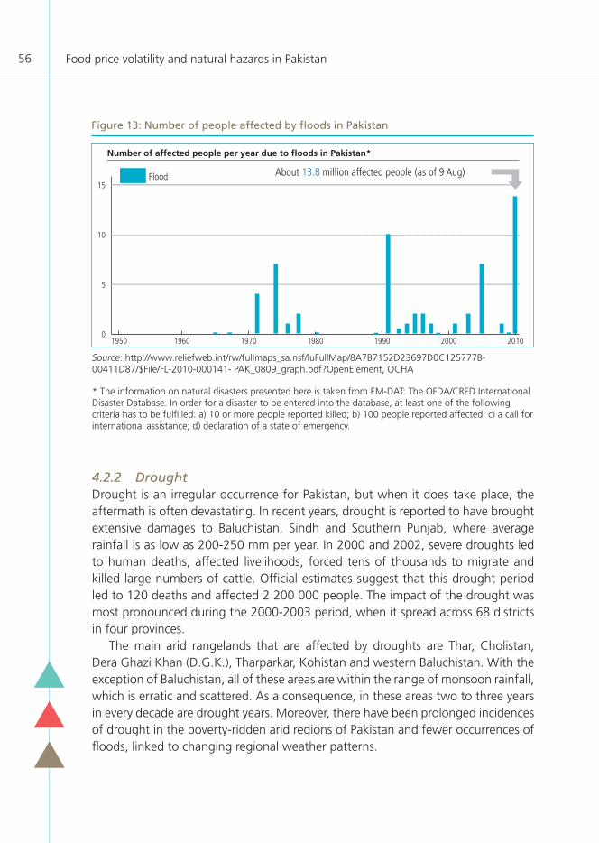
Food price volatility and natural hazards in Pakistan56
4.2.2 DroughtDrought is an irregular occurrence for Pakistan, but when it does take place, the aftermath is often devastating. In recent years, drought is reported to have brought extensive damages to Baluchistan, Sindh and Southern Punjab, where average rainfall is as low as 200-250 mm per year. In 2000 and 2002, severe droughts led to human deaths, affected livelihoods, forced tens of thousands to migrate and killed large numbers of cattle. Official estimates suggest that this drought period led to 120 deaths and affected 2 200 000 people. The impact of the drought was most pronounced during the 2000-2003 period, when it spread across 68 districts in four provinces.
The main arid rangelands that are affected by droughts are Thar, Cholistan, Dera Ghazi Khan (D.G.K.), Tharparkar, Kohistan and western Baluchistan. With the exception of Baluchistan, all of these areas are within the range of monsoon rainfall, which is erratic and scattered. As a consequence, in these areas two to three years in every decade are drought years. Moreover, there have been prolonged incidences of drought in the poverty-ridden arid regions of Pakistan and fewer occurrences of floods, linked to changing regional weather patterns.
Source: http://www.reliefweb.int/rw/fullmaps_sa.nsf/luFullMap/8A7B7152D23697D0C125777B-00411D87/$File/FL-2010-000141- PAK_0809_graph.pdf?OpenElement, OCHA
* The information on natural disasters presented here is taken from EM-DAT: The OFDA/CRED International Disaster Database. In order for a disaster to be entered into the database, at least one of the following criteria has to be fulfilled: a) 10 or more people reported killed; b) 100 people reported affected; c) a call for international assistance; d) declaration of a state of emergency.
Figure 13: Number of people affected by floods in Pakistan
About 13.8 million affected people (as of 9 Aug)
0
5
10
15Flood
2010200019901980197019601950
Number of affected people per year due to floods in Pakistan*

Chapter 4. Vulnerability to natural risks, shocks and hazards 57
4.2.3 Implications for agricultural productionFloods and droughts in Pakistan have caused tremendous damage to livelihoods and infrastructure, with severe implications for food security. As exemplified by the August 2010 flood, the largest losses and impact were suffered by the agriculture, livestock, and fisheries sectors. Damage to the already old irrigation infrastructure caused by the 2010 floods, combined with the increasing scarcity of water resources in Pakistan, pose serious risks to agricultural production. This is particularly alarming when a large portion of the national wheat output depends on irrigation.
4.3 Forecasting the impact of weather shocks on wheat productionAs shown above, Pakistan has experienced several catastrophic floods over the past few decades, which often have substantial impacts. The following crop production model determines the depth of the relationship between rainfall and wheat production by province, and provides implications for household food security. This section first reviews the descriptive statistics on the trends in wheat and rainfall data among the four main wheat producing provinces. This analysis provides the parameters for crop production monitoring, taking into account the impacts of weather related variables such as rainfall. The estimated productions are then used in the SISMOD.
4.3.1 Trends in wheat production from 1970-2008Figure 14 shows the general trend in wheat production and yield in Pakistan from 1970-2010. Both production and yield have more than doubled (increased by 2.32 times) within this time period. During these 40 years the national wheat production increased from an annual 6.85 million tonnes in 1970-72 to 22.77 million tonnes in 2008-10, an increase of 232 percent.
The main increase was the result of both a yield increase (by 120 percent) and an area increase (by 50 percent). The increase in productivity during this period was partially due to the agricultural policies and reforms implemented subsequent to the Green Revolution of the 1970s.
At a provincial level (see Figure A1.1), in Punjab production increased by 2.5 times, yield doubled, and cultivated area became 50 percent more than it used to be in 1970. There has been a steady pace in the increase in both wheat production and yield in Punjab, although a small decline was experienced from 2001 to 2003. In Sindh, from 1970 to 2000 production tripled and yield more than doubled, whereas cultivated area remained constant throughout this period. From 2000 to 2004, Sindh experienced a significant decline in both production and yield. From 2004 to 2008, production and yield went up by 60 percent and 40 percent respectively, whereas the cultivated area increased by 10 percent. Overall, wheat

Food price volatility and natural hazards in Pakistan58
production exhibited the lowest standard deviation in KPK, suggesting that this province is less likely to suffer from erratic rainfall patterns and natural disasters. For KPK, production almost tripled and yield more than doubled, while cultivated area only rose slightly from 1970 to 2008. There was a steep decline in both production and yield from 1998 to 2001, followed by an increase.
Both production and yield in Baluchistan have gone up significantly, with production being 5 times higher and yield being 2.5 times higher in 2008 than in 1970, while the cultivated area doubled. There was a steep decline in both production and yield from 1997 to 2000 in Baluchistan, followed by an increase from 2000 to 2004, and a rapid increase from 2006 to 2008.
There are considerable differences in the area cultivated across the provinces (Table 14). Baluchistan has the lowest mean of area cultivated and Punjab has the highest. Out of the four provinces, Punjab is subject to the highest fluctuation in the area cultivated since the standard deviation is extremely high. The mean representing the cultivated area is the largest for Punjab among the provinces, totaling 5 440.17 hectares. This figure is more than double the mean of the combined cultivated areas of the other 3 provinces (Baluchistan, KPK and Sindh) (2 016.43 hectares).
The fact that the median values are almost always greater than the mean values for production, area and yield implies that the impact of weather shocks related to erratic annual rainfall could have led to a decline in wheat production and yield across the various provinces in recent years. This explanation is consistent with the increase in both frequency and scale of natural disasters that have struck Pakistan in recent years.
Figure 14: General trend in wheat production and yield in Pakistan (1970-2010)
Whe
at a
rea
(mis
sion
ha)
and
pro
duct
ion
(mill
ion
tonn
es)
Whe
at y
ield
(ton
nes/
ha)
5
7
9
11
13
15
17
19
21
23
25
0.0
0.5
1.0
1.5
2.0
2.5
3.0
2010
2008
2006
2004
2002
2000
1998
1996
1994
1992
1990
1988
1986
1984
1982
1980
1978
1976
1974
1972
1970
YieldAreaProduction

Chapter 4. Vulnerability to natural risks, shocks and hazards 59
4.3.2 Trends in rainfall patterns from 1970-2010From Table 15, Sindh and Baluchistan appear to be drier areas while KPK and Punjab are wetter areas, based on rainfall over a 35-year period. The data indicate there is a great deal of variation in the rainfall pattern between the four provinces as well as within a given province.
Sindh is the driest among the four provinces, while KPK province is the wettest province, receiving the highest average annual rainfall over a 35-year period. The mean, standard deviation, minimum, maximum and median values for Sindh are the lowest among the four provinces. The data highlight that Sindh is more vulnerable to droughts. On the other hand, KPK has the highest mean, standard deviation, minimum, maximum and median values of the four provinces, suggesting that the KPK is more prone to flooding.
The range in the monthly precipitation received within a province is also quite significant, especially in KPK in Punjab, as can be seen from the differences between the minimum and maximum values. It should also be noted that owing to the vast surface area of Punjab, it might be more useful to aggregate the data at a district level, in order to better account for the variation in the rainfall data at the provincial level.
Table 14: Wheat area (000 ha), yield (tonnes/ha), and production (000 tonnes) by
province (1970-2008)
MeanStandard deviation
Minimum Maximum Median
BALUCHISTAN
Production 483.4 269.9 68.6 930.1 529.5
Area 272.2 86.1 134.5 430.5 293.7
Yield 1.63 0.59 0.40 2.41 1.86
KPK
Production 921.9 248.3 331.2 1356.0 962.2
Area 767.8 75.3 589.6 918.1 781.9
Yield 1.18 0.25 0.56 1.54 1.20
PUNJAB
Production 10575.1 3893.7 4948.2 17853.0 10513.8
Area 5440.2 707.3 4216.3 6483.4 5589.4
Yield 1.89 0.48 1.13 2.78 1.86
SINDH
Production 2077.6 592.6 1081.1 3411.4 2130.9
Area 976.5 111.0 755.5 1144.2 1010.7
Yield 2.11 0.52 1.19 3.47 2.12

Food price volatility and natural hazards in Pakistan60
Table 15: Cumulative rainfall (October-April in mm) by province (1975-2010)
Province Baluchistan KPK Punjab Sindh
Mean 105.23 341.91 218.63 29.36
Standard Deviation 55.10 145.94 107.02 27.03
Minimum 21.15 79.40 79.63 2.18
Maximum 224.87 657.00 600.26 134.24
Median 97.59 339.68 189.20 21.16
Looking at the data showing the cumulative annual rainfall for the four provinces (1975-2010), Baluchistan and Sindh are still the drier areas whereas KPK and Punjab receive more rainfall (Figure 15).
4.3.3 Provinces vulnerable to weather shocks on wheat production From this trend data, we were able to run regressions and derive the parameter estimations to link rainfall to crop yield. Detrended wheat yield and cumulative rainfall are plotted in Figure 16. The strength of the relationship between cumulative rainfall and annual wheat production is represented by the power of the regression, the R² value. The derived parameters are shown in Table 16 and the scatter plots are displayed in Figure A1.2.
The results show all four regions have a stronger correlation between estimated and observed yield when the weather shock data (droughts and floods) are
Figure 15: Cumulative rainfall (October-April) from 1975-2010 for four provinces
Punjab
Sindh Baluchistan
NWFP
mill
imet
ers
1975
1977
1979
1981
1983
1985
1987
1989
1991
1993
1995
1997
1999
2001
2003
2005
2007
2009
0
100
200
300
400
500
600
700
Rainfall pattern in four provinces at the start of the winter wheat harvest season in April, based on Pakistan’s crop calendar (using cumulative rain (October- April)

Chapter 4. Vulnerability to natural risks, shocks and hazards 61
Figure 16: Detrended wheat yield and cumulative rainfall (October-April) from 1975-2010 for four provinces
BA
LUC
HIS
TAN
SIN
DH
KPK
PUN
JAB
0
50
100
150
200
250
-0.4
-0.6
-0.2
0
0.2
0.4
0.6
2010
2008
2006
2004
2002
2000
1998
1996
1994
1992
1990
1988
1986
1984
1982
1980
1978
1976
1974
Cum
ulat
ive
rain
fall
(mm
)
Det
rend
ed w
heat
yie
ld (t
onne
s/ha
0
100
200
300
400
500
600
700
-0.5
-0.4
-0.3
-0.2
-0.1
0
0.1
0.2
Cum
ulat
ive
rain
fall
(mm
)
Det
rend
ed w
heat
yie
ld (t
onne
s/ha
)
2010
2008
2006
2004
2002
2000
1998
1996
1994
1992
1990
1988
1986
1984
1982
1980
1978
1976
1974
-0.6
-0.4
-0.2
0
0.6
0.4
0.8
Det
rend
ed w
heat
yie
ld (t
onne
s/ha
)
0.2
0.0
20
40
60
80
100
120
140
160
Cum
ulat
ive
Rain
fall
(mm
)
2010
2008
2006
2004
2002
2000
1998
1996
1994
1992
1990
1988
1986
1984
1982
1980
1978
1976
1974
0.0
-0.3-0.4
-0.2
-0.1
0
0.1
0.2
0.3
0.4
100
200
300
400
500
600
700
2010
2008
2006
2004
2002
2000
1998
1996
1994
1992
1990
1988
1986
1984
1982
1980
1978
1976
1974
Cum
ulat
ive
Rain
fall
(mm
)
Det
rend
ed w
heat
yie
ld (t
onne
s/ha
)
Cumulative rainfall (mm)Detrend yield (tonnes/ha)

Food price volatility and natural hazards in Pakistan62
excluded from the correlation. The overall trend displays a positive slope indicating that production and yield have both improved despite the frequent ups and downs caused by weather shocks. The strongest relationships were in Punjab and Sindh. Both provinces receive the largest amount of rainfall among the provinces. KPK produces the least amount of wheat, while Punjab is the largest wheat producer. The forecasting model is a good predictor of trends in crop production and yield, as is supported by the relatively high R² values. Once rainfall data that are categorized as “outliers” are removed (in order to isolate natural disaster events such as droughts or floods), the R² values increase significantly.
In conclusion, in all four provinces wheat production is vulnerable to both flood and drought shocks. The derived parameters will serve to estimate changes in wheat production in the SISMOD. The correlation between wheat production and cumulative rainfall is statistically significant, suggesting that cumulative rainfall is a good predictor of wheat production in Pakistan. This vulnerability to weather shocks has implications on household food insecurity and livelihoods in Pakistan. However, the magnitude of the impact transmitted to households largely depends on their livelihood and reliance on the agricultural sector. The next chapter provides further insights into livelihoods, incomes and consumption patterns and their vulnerability to both the market and weather shocks, identified in Chapters 3 and 4.
Table 16: Relationship between wheat yield and cumulative rainfall
(October-April) with or without shocks (droughts/floods Pakistan)
Province Estimated yield, yCoefficient of
observed yield, xConstant
Power of regression, R2
Punjab w/ weather shocks 0.92 0.16 0.91
w/o weather shocks 0.97 0.06 0.94
Sindh w/ weather shocks 0.81 0.42 0.81
w/o weather shocks 0.81 0.42 0.81
KPK w/ weather shocks 0.64 0.45 0.66
w/o weather shocks 0.71 0.36 0.80
Baluchistan w/ weather shocks 0.59 0.73 0.64
w/o weather shocks 0.58 0.74 0.66

5. Household food security and vulnerability to shocks
63
The last aspect of the profiling analyses livelihood groups that are vulnerable to potential shocks. In order to provide such an assessment, this chapter presents a descriptive household analysis. The analysis groups the different profiles by province and by livelihood in rural and urban areas, including demographics, income sources, assets (land and livestock), expenditures and food energy consumption. These variables provide insight into sectors of the population in Pakistan that are more vulnerable to the impacts of market and climate shocks.
5.1 Demographics
5.1.1 Nationwide demographicsPakistan is the sixth most populous country in the world, with an estimated population of about 170 million people. The population is still growing quite significantly, with a growth rate of 2.05 percent over the last four years. Pakistan is considered a “young” country, as there are currently 104 million Pakistanis below the age of thirty. Approximately 109.1 million people reside in rural areas and 60.9 million live in cities. Life expectancy in Pakistan is 64.1 years of age (GOP, 2010).
Pakistan is currently the most urbanized nation in South Asia. Urban dwellers make up 36 percent of the population. Since 1950, Pakistan’s urban population has expanded seven-fold, while the total population increased four-fold. The urbanization growth rate is 3 percent (GOP, 2010).
Pakistan has the tenth largest labor force in the world. According the latest Labor Force Survey of 2008-2009, the labor force is estimated at about 54 million. The total working-age population is 121 million. Of the total labor force, about three million people are unemployed, which results in unemployment rate of 5.5 percent. The gender distribution of the labor force is 42 million men and 12 million women (GOP, 2010).
5.1.2 Demographics of the household survey sampleThe descriptive analyses of demographics in different livelihood groups in Pakistan show many similarities between rural and urban areas (Table A1.11). The household sizes range between 7 and 15 persons in rural areas and 7 and 12 persons in urban areas. However, rural areas exhibit a relatively higher dependency ratio compared
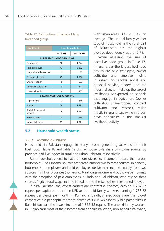
Food price volatility and natural hazards in Pakistan64
with urban areas, 0.49 vs. 0.42, on average. The unpaid family worker type of household in the rural part of Baluchistan has the highest average dependency ratio of 0.78.
When assessing the size of each livelihood group in Table 17. In rural areas the largest livelihood groups are paid employee, owner cultivator and employer, while in urban households social and personal service, traders and the industrial sector make up the largest livelihoods. As expected, households that engage in agriculture (owner cultivator, sharecropper, contract cultivator, and livestock) reside mostly in rural areas, while in urban areas agriculture is the smallest livelihood activity.
5.2 Household wealth status
5.2.1 Income by source Households in Pakistan engage in many income-generating activities for their livelihoods. Table 18 and Table 19 display households share of income sources by province and livelihoods in rural and urban Pakistan, respectively.
Rural households tend to have a more diversified income structure than urban households. Their income sources are spread among two to three sources. In general, households of employers and paid employees derive their incomes mainly from two sources in all four provinces (non-agricultural wage income and public wage income), with the exception of paid employees in Sindh and Baluchistan, who rely on three sources (agricultural wage income in addition to the two others mentioned above).
In rural Pakistan, the lowest earners are contract cultivators, earning 1 287.07 rupees per capita per month in KPK and unpaid family workers, earning 1 733.22 rupees per capita per month in Punjab. In Sindh, sharecroppers are the lowest earners with a per capita monthly income of 1 815.48 rupees, while pastoralists in Baluchistan earn the lowest income of 1 862.58 rupees. The unpaid family workers in Punjab earn most of their income from agricultural wage, non-agricultural wage,
Table 17: Distribution of households by
livelihood group
Livelihood Rural households
% of HH No. of HH
RURAL LIVELIHOOD GROUPING
Employer 16 1 224
Paid employee 43 3 322
Unpaid family worker 1 63
Owner cultivator 25 1 916
Share cropper 9 693
Contract cultivator 3 217
Livestock only 4 307
URBAN LIVELIHOOD GROUPING
Agriculture 7 346
Traders 26 1 291
Social & personal service
29 1 463
Service sector 13 639
Industrial sector 25 1 221

Chapter 5. Household food security and vulnerability to shocks 65
Table 18: Per capita monthly income (Rs) and percentage share by source and by
livelihood group in rural areas in Pakistan
Note: Livelihood Groups of Unpaid family worker and Contract Cultivator in Baluchistan are not shown since only very small samples were available
LivelihoodPer capita
incomeCrop
incomeLivestock income
Agricultural wage
income
Non agricultural
wage
Public wage
Remittance income
Other income
Rs .............................................................................. % ..............................................................................
PUNJAB
Employer 2 475 2.5 5.8 4.7 57.4 22.8 2.8 4.1
Paid employee 2 024 2.2 6.6 11.3 50.5 23.5 3.2 2.8
Unpaid family worker
1 733 8.5 15.8 35.3 16.1 6.3 14.6 3.4
Owner cultivator 3 298 15.8 18.1 52.3 5.6 2.3 4.2 1.8
Sharecropper 1 946 11.0 21.1 50.4 8.7 1.3 6.0 1.4
Contract cultivator
2 996 22.5 17.3 48.6 6.0 1.2 3.5 0.8
Livestock only 2 357 0.1 37.2 30.8 9.6 1.8 9.2 11.3
SINDH
Employer 2 604 3.0 8.8 8.7 62.9 11.5 0.1 5.0
Paid employee 2 017 3.8 3.0 29.8 39.9 20.0 0.1 3.5
Unpaid family worker
2 537 34.3 5.6 54.8 3.5 0.3 1.5 0.0
Owner cultivator 2 869 27.7 9.6 53.6 5.0 2.9 0.3 0.9
Sharecropper 1 815 27.4 10.0 51.2 8.1 2.8 0.4 0.2
Contract cultivator
3 004 27.4 2.9 59.7 5.0 4.9 0.0 0.0
Livestock only 3 149 0.7 13.6 20.9 2.4 1.3 0.4 60.7
KPK
Employer 2 470 0.9 2.7 2.2 55.8 22.4 7.8 8.2
Paid employee 1 975 1.6 3.2 4.8 49.1 27.6 6.9 6.6
Unpaid family worker
1 443 -7.4 5.4 17.7 33.3 13.9 23.1 14.1
Owner cultivator 1 759 5.8 15.0 38.4 10.8 6.0 19.5 4.4
Sharecropper 1 521 6.3 19.8 37.1 16.0 3.8 14.9 2.0
Contract cultivator
1 287 3.6 14.3 45.1 12.2 6.4 15.2 3.2
Livestock only 2 211 1.1 39.0 34.0 7.9 3.2 12.6 2.2
BALOCHISTAN
Employer 2 514 1.7 1.6 9.7 58.6 25.7 0.1 2.6
Paid employee 2 020 2.7 1.8 14.9 49.6 29.0 0.3 1.7
Owner cultivator 2 570 14.1 4.4 67.4 8.3 5.0 0.4 0.5
Sharecropper 2 165 17.5 9.6 67.4 2.3 2.2 0.0 0.9
Livestock only 1 863 0.7 31.3 40.5 8.8 4.6 2.2 11.9

Food price volatility and natural hazards in Pakistan66
and livestock income; in Sindh most of the sharecroppers earn through both crop income and agricultural wage income; and in Khyber Pakhtunkhwa agricultural wage, remittance income, livestock and non-agricultural wage income prevails for contract cultivators.
Urban household income is generally distributed among one to three income sources. Among the urban livelihood groups, more than 80 percent of income share is derived from non-agricultural wages and public wages in all four provinces, with the exception of the agriculture-based households. The service sector captures the highest income levels in Punjab, Sindh, and KPK. Service sector based households in urban Punjab capture the highest per capita total monthly income of 4 866 rupees, with public and non-agricultural wages accounting for roughly 90 percent of the incomes. This is closely followed by agriculture-based households in Punjab, earning a per capita total monthly income of 4856.80 rupees. The per capita wages are generally lower in Baluchistan than in the other provinces for all sectors with the exception of agriculture-based households, which have the highest income levels in Baluchistan, at 3 256 rupees.
Similar to rural households, urban households classified as agriculturalists tend to have more diversified income structures than non-agricultural households. In urban agricultural households, the main share of income range from two to three sources, typically from agricultural wages, livestock, and non-agricultural wages, depending on the province. The agriculture livelihood groups in both Baluchistan and KPK have a well-distributed share of income across sources.
5.2.2 Income by cropTable 20 and Table A1.12 provide more details in terms of crop income earned by province and by livelihoods in rural and urban areas, respectively. As previously stated, rural areas are mostly engaged in agricultural activities and hence earn the most crop income. Wheat is a very important crop in Pakistan and most livelihood groups in all provinces engage in wheat production. Punjab and Sindh earn crop income from the production of wheat, rice, cotton and sugar. The biggest earners from maize are contract cultivators in Punjab and owner cultivators in KPK, while it is sharecropper households in Punjab and Baluchistan for pulses. Earnings from fruit production come from urban farming in Baluchistan and Pujab, and owner cultivators in Baluchistan.
5.2.3 Asset ownershipAsset ownership is a good determinant of household wealth. Table A1.13 and Table A1.14 show livelihoods and assets by province in rural and urban households, respectively. As expected, owner cultivators own the most land in rural Pakistan.

Chapter 5. Household food security and vulnerability to shocks 67
Table 19: Per capita monthly income (Rs) and percentage share by source in urban areas
in Pakistan
LivelihoodPer capita
incomeCrop
incomeLivestock income
Agricultural wage
income
Non agricultural
wage
Public wage
Remittance income
Other income
Rs ................................................................................% ...............................................................................
PUNJAB
Agriculture 4 857 4.8 16.4 55.6 7.9 4.7 3.3 7.2
Traders 3 913 0.4 2.4 0.7 85.2 5.4 1.8 4.2
Social & personal service
4 850 0.4 0.9 0.9 46.4 42.7 2.0 6.6
Service sector 4 866 0.6 0.2 0.2 18.9 70.5 3.8 5.7
Industrial sector 3 895 0.4 0.9 0.4 89.3 4.6 1.6 2.9
SINDH
Agriculture 3 097 13.2 5.9 67.7 7.1 3.4 0.0 2.6
Traders 4 673 0.0 0.2 0.0 90.7 5.6 0.5 2.9
Social & personal service
4 064 0.1 0.2 0.2 51.3 45.4 0.2 2.6
Service sector 4 682 0.0 0.2 0.3 10.9 87.3 0.0 1.3
Industrial sector 4 414 0.0 0.1 0.2 90.7 5.1 0.1 3.7
KPK
Agriculture 2 572 2.8 16.1 39.5 15.9 9.6 5.5 10.6
Traders 3 127 0.0 0.7 0.5 86.2 4.5 2.4 5.7
Social & personal service
3 661 0.0 0.4 1.2 46.6 42.1 2.8 6.8
Service sector 4 272 0.2 0.9 0.8 7.1 79.8 5.5 5.8
Industrial sector 3 348 0.0 0.8 0.3 79.4 8.0 1.8 9.6
BALUCHISTAN
Agriculture 3 256 10.3 9.2 63.8 8.9 7.1 0.5 0.2
Traders 2 402 0.0 0.6 1.4 88.4 6.7 0.9 2.0
Social & personal service
2 975 0.0 0.2 1.0 49.0 48.2 0.0 1.7
Service sector 2 577 0.0 0.1 0.0 7.3 91.3 0.2 1.1
Industrial sector 2 894 0.0 0.1 0.3 89.0 6.7 0.0 3.9
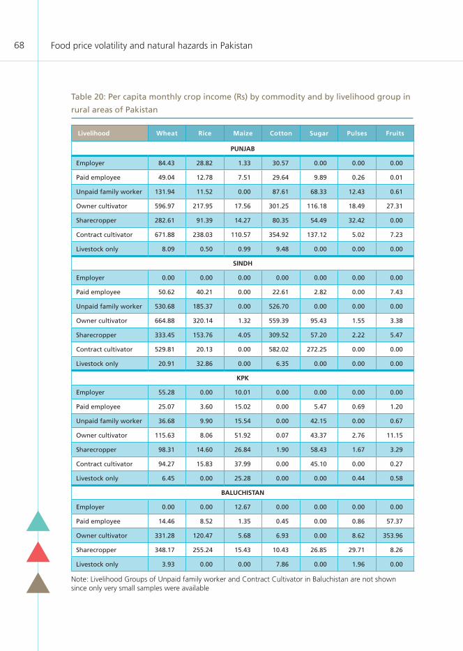
Food price volatility and natural hazards in Pakistan68
Table 20: Per capita monthly crop income (Rs) by commodity and by livelihood group in
rural areas of Pakistan
Livelihood Wheat Rice Maize Cotton Sugar Pulses Fruits
PUNJAB
Employer 84.43 28.82 1.33 30.57 0.00 0.00 0.00
Paid employee 49.04 12.78 7.51 29.64 9.89 0.26 0.01
Unpaid family worker 131.94 11.52 0.00 87.61 68.33 12.43 0.61
Owner cultivator 596.97 217.95 17.56 301.25 116.18 18.49 27.31
Sharecropper 282.61 91.39 14.27 80.35 54.49 32.42 0.00
Contract cultivator 671.88 238.03 110.57 354.92 137.12 5.02 7.23
Livestock only 8.09 0.50 0.99 9.48 0.00 0.00 0.00
SINDH
Employer 0.00 0.00 0.00 0.00 0.00 0.00 0.00
Paid employee 50.62 40.21 0.00 22.61 2.82 0.00 7.43
Unpaid family worker 530.68 185.37 0.00 526.70 0.00 0.00 0.00
Owner cultivator 664.88 320.14 1.32 559.39 95.43 1.55 3.38
Sharecropper 333.45 153.76 4.05 309.52 57.20 2.22 5.47
Contract cultivator 529.81 20.13 0.00 582.02 272.25 0.00 0.00
Livestock only 20.91 32.86 0.00 6.35 0.00 0.00 0.00
KPK
Employer 55.28 0.00 10.01 0.00 0.00 0.00 0.00
Paid employee 25.07 3.60 15.02 0.00 5.47 0.69 1.20
Unpaid family worker 36.68 9.90 15.54 0.00 42.15 0.00 0.67
Owner cultivator 115.63 8.06 51.92 0.07 43.37 2.76 11.15
Sharecropper 98.31 14.60 26.84 1.90 58.43 1.67 3.29
Contract cultivator 94.27 15.83 37.99 0.00 45.10 0.00 0.27
Livestock only 6.45 0.00 25.28 0.00 0.00 0.44 0.58
BALUCHISTAN
Employer 0.00 0.00 12.67 0.00 0.00 0.00 0.00
Paid employee 14.46 8.52 1.35 0.45 0.00 0.86 57.37
Owner cultivator 331.28 120.47 5.68 6.93 0.00 8.62 353.96
Sharecropper 348.17 255.24 15.43 10.43 26.85 29.71 8.26
Livestock only 3.93 0.00 0.00 7.86 0.00 1.96 0.00
Note: Livelihood Groups of Unpaid family worker and Contract Cultivator in Baluchistan are not shown since only very small samples were available

Chapter 5. Household food security and vulnerability to shocks 69
Contract cultivators and sharecroppers rent the most land in rural Pakistan, while sharecroppers mostly dispose of shared land. In urban Pakistan, agriculture-based urban households mostly own land; they rent and share land to a minimal extent. In Baluchistan, there is no evidence of any land rental or shared land.
In terms of total annual per capita livestock owned, unpaid family workers in rural KPK account for the highest value of 51 827 rupees (Table A1.13); but most of this is not marketed (as they account for a low per capita monthly livestock income of 78 rupees, equivalent to 5 percent share of total income, see Table 18). Buffaloes account for most of this value.
Pastoralist-based households have total per capita value of livestock owned ranging between 10 738 rupees/year in rural KPK and 15 375 rupees/year in rural Sindh (Table A1.13). Comparing with incomes, we observe that earnings from livestock account for about 39 percent of the total income of Pastoralist-based households in KPK while they account for 13.6 percent in Sindh (Table 18).
In urban areas, agriculture-engaged households possess the highest per capita livestock value, as is to be expected: 13 909 rupees/year in Punjab; 5 562 rupees/year in Sindh; 3 782 rupees/year in KPK; and 1 884 rupees/year in Baluchistan (Table A1.14). Buffalo (70 percent) and cattle (21 percent) make up most of the livestock asset value.
5.3 Household food consumption
5.3.1 ExpendituresThe analysis of expenditures is displayed in Table A1.15 for rural households and in Table A1.16 for urban households. Employers are among those having the highest expenditure levels in all rural regions, as expected, since employers are among the highest income earners. Owner cultivators in Punjab, pastoralists in Sindh, and unpaid family workers in KPK also have high per capita expenditure levels, which correlate to their high income levels.
In general, for the average household, 60 percent of expenditures are allocated to non-food items and 40 percent to food items. Employers spend the most on food items (on average 471 rupees per month), but have an average distribution of expenditures between food (40 percent) and non-food items (60 percent). In urban areas, agricultural households spend the least on food items and allocate slightly less of their expenditures to food (on average 38 percent). However, the percentage of food expenditures varies quite significantly by livelihood group and by province. For example, while contract cultivators in Sindh spend 42 percent of their total income on food, those in KPK spend 47 percent on food items.

Food price volatility and natural hazards in Pakistan70
5.3.2 Food calorie intakeTable A1.17 and Table A1.18 display livelihoods and food calorie intake by province in rural and urban areas, respectively. The top 5 livelihoods in terms of total per capita calorie intake are agricultural households in urban Punjab and KPK (2 930 kcal and 2 697 kcal), owner cultivators in rural Punjab (2 925 kcal), pastoralists in rural KPK (2 808 kcal), and contract cultivators in rural Punjab (2 690 kcal).
The bottom 5 livelihoods in terms of total per capita calorie intake are mostly in urban Baluchistan: agricultural households (1 879 kcal), traders (1 792 kcal), service sector (2 007 kcal) and social and personal service (2 016 kcal). For rural areas, paid employees in rural Sindh have the lowest caloric intake of 1 984 kcal per capita.
The food items that make up most of the calorie intake in Pakistan are wheat, milk and rice, which account for 55 percent of caloric intake for the average rural household and 49 percent among urban dwellers. High-income groups tend to consume different food items compared with medium and low-income groups. In rural areas in Pakistan, high-income groups consume more milk, sugar, fats and oils, and fruit than medium- and low-income groups. The main difference in urban areas is that there are more equal consumption patterns of sugar between low- and high-income groups.
5.3.3 UndernourishmentThe Percentage of people consuming less than the DECR is measured by comparing the usual food consumption expressed in terms of dietary energy (kcal) with the energy requirement norm of 2 350 kcal, which is the adult calorie requirement. The part of the population with food consumption below the energy requirement norm is considered undernourished.
Table 21 summarizes the undernourishment status in Pakistan. Rural Punjab has the highest average per capita total food calorie intake of 2 571.27 kcal, while, urban Baluchistan the smallest, of 2 019.63 kcal, with an estimated 67 percent of its population undernourished. Overall, the Pakistan average is satisfactory at 2 372.10 kcal, although about 45 percent of the population is undernourished in the baseline survey data.
Tables 22 and 23 display undernourishment among livelihood groups in rural and urban areas in Pakistan. Employers comprise a relatively low proportion of undernourished households as they are the highest income earners as well as spenders on food. The lowest levels of undernourishment (i.e. below 2 350 kcal) are encountered in households involved in the agricultural sectors. This is with the exception of owner cultivators, sharecroppers, pastoralists in rural Baluchistan (50 percent, 53 percent, and 60 percent of undernourished, respectively), and sharecroppers in rural Sindh (48 percent of undernourished, below 2 350 kcal), and
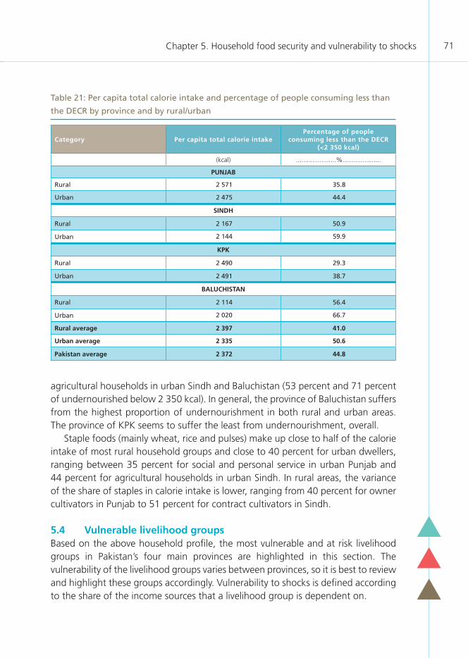
Chapter 5. Household food security and vulnerability to shocks 71
Table 21: Per capita total calorie intake and percentage of people consuming less than
the DECR by province and by rural/urban
Category Per capita total calorie intakePercentage of people
consuming less than the DECR (<2 350 kcal)
(kcal) ......................%.....................
PUNJAB
Rural 2 571 35.8
Urban 2 475 44.4
SINDH
Rural 2 167 50.9
Urban 2 144 59.9
KPK
Rural 2 490 29.3
Urban 2 491 38.7
BALUCHISTAN
Rural 2 114 56.4
Urban 2 020 66.7
Rural average 2 397 41.0
Urban average 2 335 50.6
Pakistan average 2 372 44.8
agricultural households in urban Sindh and Baluchistan (53 percent and 71 percent of undernourished below 2 350 kcal). In general, the province of Baluchistan suffers from the highest proportion of undernourishment in both rural and urban areas. The province of KPK seems to suffer the least from undernourishment, overall.
Staple foods (mainly wheat, rice and pulses) make up close to half of the calorie intake of most rural household groups and close to 40 percent for urban dwellers, ranging between 35 percent for social and personal service in urban Punjab and 44 percent for agricultural households in urban Sindh. In rural areas, the variance of the share of staples in calorie intake is lower, ranging from 40 percent for owner cultivators in Punjab to 51 percent for contract cultivators in Sindh.
5.4 Vulnerable livelihood groupsBased on the above household profile, the most vulnerable and at risk livelihood groups in Pakistan’s four main provinces are highlighted in this section. The vulnerability of the livelihood groups varies between provinces, so it is best to review and highlight these groups accordingly. Vulnerability to shocks is defined according to the share of the income sources that a livelihood group is dependent on.

Food price volatility and natural hazards in Pakistan72
LivelihoodPercentage of people
consuming less than the DECR (<2,350 Kcal)
Share of staple food consumption in calorie intake
....................................%....................................
PUNJAB
Employer 41.4 42.8
Paid employee 47.9 44.2
Unpaid family worker 40.6 46.1
Owner cultivator 23.2 40.1
Sharecropper 19.6 43.3
Contract cultivator 24.9 41.6
Livestock only 28.5 41.7
SINDH
Employer 32.9 45.3
Paid employee 57.1 46.5
Unpaid family worker 41.8 44.1
Owner cultivator 35.8 45.5
Sharecropper 47.9 49.8
Contract cultivator 41.8 50.5
Livestock only 34.0 44.4
KPK
Employer 23.8 44.8
Paid employee 35.1 45.1
Unpaid family worker 27.0 40.6
Owner cultivator 20.1 45.8
Sharecropper 28.6 44.2
Contract cultivator 38.9 48.2
Livestock only 18.0 40.7
BALUCHISTAN
Employer 63.7 46.1
Paid employee 58.3 47.8
Owner cultivator 49.6 45.7
Sharecropper 53.1 48.3
Livestock only 60.1 47.5
Table 22: Percentage of people consuming less than the DECR and share of staple food
consumption in rural Pakistan by livelihood group and province
Note: Livelihood Groups of Unpaid family worker and Contract Cultivator in Baluchistan are not shown since only very small samples were available

Chapter 5. Household food security and vulnerability to shocks 73
There are three main income sources: crop and livestock income, agricultural wage income and non-agricultural wage income. Livelihood groups (owner cultivator, sharecropper, contract cultivator and pastoralists) whose major income source (at least 1/3) is crop and livestock income would be vulnerable to both market and climate shocks. Those that receive a significant portion of their income (at least 1/3) from agricultural wage income are at risk of both market and climatic shocks, as they would be dependent on the market for food expenditures and their agricultural wage labor could be affected in the case of a climate shock (flood,
Table 23: Percentage of people consuming less than the DECR and share of staple food
consumption in urban Pakistan by livelihood group and province
LivelihoodPercentage of people
consuming less than the DECR (<2 350 kcal)
Share of staple food consumption in calorie intake
....................................%....................................
PUNJAB
Agriculture 23.0 36.9
Traders 51.4 36.6
Social & personal service 42.5 35.0
Service sector 47.1 36.8
Industrial sector 51.2 38.7
SINDH
Agriculture 53.0 43.6
Traders 59.1 37.6
Social & personal service 61.1 38.2
Service sector 58.2 37.3
Industrial sector 58.8 38.5
KPK
Agriculture 34.2 42.3
Traders 43.8 40.6
Social & personal service 32.0 36.4
Service sector 31.2 40.6
Industrial sector 38.9 41.4
BALUCHISTAN
Agriculture 70.9 42.7
Traders 70.6 43.3
Social & personal service 63.1 41.9
Service sector 61.9 43.0
Industrial sector 59.4 42.5

Food price volatility and natural hazards in Pakistan74
Table 24: Vulnerability of rural livelihood groups to shocks
Level of Vulnerability to Shocks - XXX: High (> 1/3 of incomes); XX: Moderate (10-33% of incomes); X: Low (<10% of incomes
Livelihood Market shocks Climate shocks
PUNJAB
Employer XXX X
Paid employee XXX XX
Unpaid family worker XXX XXX
Owner cultivator XX XXX
Sharecropper XX XXX
Contract cultivator XX XXX
Livestock only XX XXX
SINDH
Employer XXX X
Paid employee XXX XX
Unpaid family worker X XXX
Owner cultivator X XXX
Sharecropper XX XXX
Contract cultivator XX XXX
Livestock only X XX
KPK
Employer XXX X
Paid employee XXX X
Unpaid family worker XXX XX
Owner cultivator XXX XX
Sharecropper XXX XXX
Contract cultivator XXX XXX
Livestock only XX XXX
BALOCHISTAN
Employer XXX X
Paid employee XXX XX
Unpaid family worker X XXX
Owner cultivator XX XXX
Sharecropper X XXX
Contract cultivator X XXX
Livestock only XX XXX

Chapter 5. Household food security and vulnerability to shocks 75
drought). Non-agricultural wage income, public wage income, and remittances would be the most vulnerable to a market shock, as their livelihoods are dependent on both domestic and international markets.
In general, employers and paid employees in rural areas (Table 24) and traders, social and personal service, service sector, and industrial workers in urban areas (Table 25) receive the majority (close to 80 percent) of their income from non-agricultural income sources as mentioned above. These livelihood groups are likely to be more
Livelihood Market shocks Climate shocks
PUNJAB
Agriculture XX XXX
Traders XXX X
Social & Personal service XXX X
Service sector XXX X
Industrial sector XXX X
SINDH
Agriculture XX XXX
Traders XXX X
Social & personal service XXX X
Service sector XXX X
Industrial sector XXX X
KPK
Agriculture XXX XXX
Traders XXX X
Social & personal service XXX X
Service sector XXX X
Industrial sector XXX X
BALUCHISTAN
Agriculture XX XXX
Traders XXX X
Social & personal service XXX X
Service sector XXX X
Industrial sector XXX X
Table 25: Vulnerability of urban livelihood groups to shocks
Level of Vulnerability to Shocks - XXX: High (> 1/3 of incomes); XX: Moderate (10-33% of incomes); X: Low (<10% of incomes

Food price volatility and natural hazards in Pakistan76
vulnerable to market shocks. Unpaid family worker, owner cultivator, sharecropper, contract cultivator and livestock livelihood groups have more distributed incomes sources between crop and livestock income, agricultural wage income, and non-agricultural wage income. These groups are likely to be more vulnerable to both climate and markets shocks.
6. Simulating the impacts of market and climate shocks on household food consumption
77
This chapter builds on the baseline profiles of Chapters 3, 4 and 5 to simulate the impacts of price increases and floods on caloric intake. The chapter begins by reviewing the main findings from the vulnerability profiling in order to depict its relation to SISMOD. This section is followed by a review of the main aspects of the methodology. The last section provides the results from SISMOD, which is organized by the Percentage of people consuming less than the DECR (categorized by rural/urban, main provinces, livelihood groups, and income groups), the number of undernourished people, and the food needs to meet the caloric requirement of the undernourished.
6.1 Overview of SISMOD: Interaction between vulnerability profiling and parameter estimationsIn the case of Pakistan, the application of the SISMOD will focus on examining the impact of previous shocks on household income, expenditure and food consumption.
6.1.1 Review of main findings from vulnerability profilingThe key findings of the vulnerability profiling portray the trajectory of market and climate shocks by exposing the key markers to these crises: changes in price and production. These pathways of the two different shock factors will determine the magnitude of the impacts on households, simulated by the SISMOD.
The results of the price transmission analysis (Chapter 3) suggests that international cereal price shocks are transmitted to the Pakistani domestic markets through Hyderabad and Peshawar for wheat, and Multan, Sukkur, Peshawar, Rawalpindi and Quetta for IRRI rice and Hyderabad for Basmatti rice. However, due to policy interventions, the speed of transmission is delayed and domestic prices are sticky to international price declines. The above leading markets also play an important role in domestic price transmission between markets.
The relationship between crop production and natural disasters also suggests that all the main wheat production areas in Pakistan are significantly vulnerable to climate shocks. The most vulnerable wheat producing areas to weather shocks are Punjab and KPK (Chapter 4).
The household profiling reveals that a household’s relationship with the agricultural sector in sustaining its livelihood plays a large role in the type of shock

Food price volatility and natural hazards in Pakistan78
and the extent to which it is likely to be affected (Chapter 5). Livelihood groups that depend on the agricultural sector (crop and livestock income; agricultural wage income) have a more distributed share of income sources among crop income, agricultural wage income and non-agricultural income, and are likely to be impacted by both market and climate shocks. Livelihoods groups that are less directly dependent on the agricultural sector and whose main incomes are sourced from non-agricultural wage are likely to be most impacted by market shocks.
6.1.2 Shock scenarios The shock model simulates two different scenarios to provide the most likely situations of market and climate shocks. The first scenario (market shock) is based on actual changes in real wholesale prices, retail prices and wage rates between 2005/06 and 2010/11. These changes were estimated for 20 commodity prices and wage rates in each province.
The second scenario combines scenario one and the impact of the flooding in August 2010. The impact of flooding is captured by the actual losses in crop and livestock production. These losses were estimated through assessments in more than 120 districts in Pakistan.
6.2 Impact of shocks on household food securityPlease note that the following sections present the simulation results for the percentage of people with daily intake <2 350 kcal/day in adult equivalents; other definitions for undernourishment such as 2 100 kcal/day and 1 730 kcal/day were also applied to all categories of the simulation results and the results are provided in Appendices 2 and 3.
6.2.1 Impacts on percentage of people consuming less than the threshold (DECR)Table 26 shows the results of the simulation applied to rural and urban areas, four provinces, seven livelihood groups, and three income groups. These results are articulated in terms of proportion of population with calorie intake below the adult equivalent for daily required kilocalories (<2 350 kcal.)10. The simulation results of scenario one (market shocks) show that price increases had a substantial impact on the Percentage of people consuming less than the DECR in both rural and urban areas (7.5 percentage points increase), but rural areas were impacted more (9.3 percentage points increase) than urban areas (4.8 percentage points increase). In
10 Other definitions for undernourishment such as, 2 100 kcal and 1 730 kcal are applied to all categories of the simulation results and provided in Appendix 2 and Appendix 3.
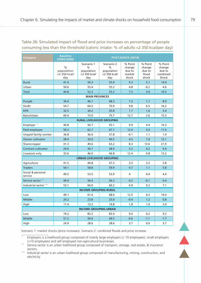
Chapter 6. Simulating the impacts of market and climate shocks on household food consumption 79
Table 26: Simulated impact of flood and price increases on percentage of people consuming less than the threshold (caloric intake: % of adults <2 350 kcal/per day)
CategoryBaseline
(2005/2006)POST-SHOCK (2010)
% population <2 350 kcal/
day
Scenario 1%
population <2 350 kcal/
day
Scenario 2%
population<2 350 kcal/
day
% Point change due to market shock
% Point change due to flood shock
% Point change due to
combined Shock
Rural 41.0 50.3 55.4 9.3 5.1 14.4
Urban 50.6 55.4 55.2 4.8 -0.2 4.6
Total 44.8 52.3 55.3 7.5 3.0 10.5
MAIN PROVINCES
Punjab 39.4 46.7 48.3 7.3 1.7 8.9
Sindh 54.7 64.5 70.9 9.8 6.5 16.2
KPK 32.5 34.2 35.8 1.7 1.6 3.4
Baluchistan 60.4 73.0 75.7 12.7 2.6 15.3
RURAL LIVELIHOOD GROUPING
Employer * 40.8 50.7 55.1 9.9 4.4 14.3
Paid employee 50.3 62.7 67.7 12.4 5.0 17.4
Unpaid family worker 36.8 36.6 37.8 -0.1 1.1 1.0
Owner cultivator 28.4 33.0 40.5 4.5 7.6 12.1
Sharecropper 41.3 49.6 63.2 8.3 13.6 21.9
Contract cultivator 29.6 34.7 38.9 5.2 4.2 9.4
Livestock only 33.6 46.0 46.8 12.4 0.8 13.2
URBAN LIVELIHOOD GROUPING
Agriculture 41.5 44.8 47.3 3.3 2.5 5.8
Traders 54.1 58.8 59.9 4.7 1.1 5.8
Social & personal service
49.5 53.5 53.9 4 0.4 4.4
Service sector ** 49.9 56.4 56.3 6.5 -0.1 6.4
Industrial sector *** 53.1 60.0 60.2 6.9 0.2 7.1
INCOME GROUPING-RURAL
Low 49.1 61.6 68.0 12.5 6.5 19.0
Middle 24.2 23.8 25.0 -0.4 1.2 0.8
High 11.4 13.2 14.8 1.8 1.6 3.4
INCOME GROUPING-URBAN
Low 74.2 83.2 83.4 9.0 0.2 9.2
Middle 51.2 50.6 49.5 -0.6 -1.1 -1.7
High 24.9 28.6 28.6 3.7 0.0 3.7
Scenario 1: market shocks (price increases). Scenario 2: combined floods and price increase.
* Employers is a livelihood group composed of mainly large employers (≥ 10 employees), small employers (<10 employees) and self employed non-agricultural businesses.
** Service sector is an urban livelihood group composed of transport, storage, real estate, & insurance sectors.
*** Industrial sector is an urban livelihood group composed of manufacturing, mining, construction, and electricity.

Food price volatility and natural hazards in Pakistan80
scenario two (combined market and flood shocks), the level of undernourishment in urban areas remained almost unchanged compared with scenario one, suggesting that urban households are less vulnerable to floods.
When categorizing the impacts by province, the results show that price increases had the largest impact in Baluchistan with a 13 percent percentage point increase. The market shock also substantially affected both Punjab and Sindh, which are the two largest wheat producing regions in Pakistan. The floods in 2010 had a significant impact only on the province of Sindh, with a 6.5 percentage point increase of undernourishment from the 2005/06 baseline scenario. The combined market and flood shocks had the highest incidence on undernourishment in Sindh (16.2 percentage points increase). KPK proved to be the most resilient to both price increases and floods. Figure 17 displays these provincial trends spatially for identifying the impacts of price increases and flooding on the Percentage of people consuming less than the DECR by district.
The results categorized by livelihood groups show similar findings from the baseline situation. Unsurprisingly, the livelihood groups that are less dependent on the agricultural sector as their main source of income are most affected by price increases in rural areas (first two rural livelihood groups in Table 26). Paid employees and pastoralists are the worst affected livelihoods, as the percentage of those having an inadequate food intake increased in both groups by 12.4 percentage points to 62.7 percent and 46.0 percent, respectively. Price increases also seem to have resulted in a substantial increase of undernourishment figures among employer-based households. The income source of employers is derived mainly from non-agricultural wages and public wages, which explains their vulnerability. Overall, household groups with agricultural production face relatively smaller impacts of price increases on the Percentage of people consuming less than the DECR. Rural non-farming households are worst hit by price increases because they cannot rely on own production for food consumption.
When applying the flood shock impact, the livelihood groups whose main income sources are derived from the agricultural sector were most affected. Sharecroppers suffered the most among the livelihood groups, having the highest percentage increase of undernourishment of 13.6 percentage points due to flooding. On average among the four provinces, sharecroppers earn over 80 percent of their income from the agricultural sector. In Baluchistan and Sindh sharecroppers have the highest shares of agriculture-based income of 94 percent and 88 percent. Owner cultivators also faced a relatively high percentage increase of undernourishment of 7.6 percentage points. Overall, rural farming households were worst hit by the August 2010 floods because they rely on production as their source of food and income.
The combined impacts of market and climate shocks seem to push households

Chapter 6. Simulating the impacts of market and climate shocks on household food consumption 81
which already had high-levels of food insecurity pre-crises into further destitution. When applying scenario two of the combined impact of price increases and floods, sharecroppers have the highest increase of undernourishment of 21.9 percentage points from the baseline year, with 63.2 percent of the population being undernourished in scenario 2. This is the second highest total inadequate food intake among livelihoods groups. Sharecroppers have quite a diverse income structure: their income comes from two to five sources in the four main provinces. Sharecroppers in KPK derive their income from five different sources. These balanced sources of income can explain this combined impact for sharecroppers. Also in scenario two, paid employees have the second highest increase in inadequate food intake of 17.4 percentage points, and the highest undernourished overall population among the livelihood groups of 67.7 percent.
Among urban livelihood groups, price increases had a larger impact on households’ undernourishment than floods, as income sources were generally derived from non-agricultural income with the exception of agricultural-based urban households. Service sector and manufacturing sector based households were
Figure 17: Percentage of people consuming less than the threshold due to simulated
market and flood shocks by district (% of population below 2 350 kcal/day)

Food price volatility and natural hazards in Pakistan82
the worst affected urban livelihoods, as inadequate food intake increased by 6.5 percentage points to 56.4 percent and by 6.9 percentage points to 60 percent respectively. The simulation results found the situation of flooding to only affect agricultural based households among the urban livelihood grouping (2.5 percentage point increase).
Looking at the income groups, the shock impact simulation shows that a larger proportion of low-income households became undernourished as a result of price increases in both rural (12.5 percentage points) and urban (9.0 percentage points) areas. In the case of flooding, only low income households in rural areas are affected (6.5 percentage points increase in rural). Middle and high income groups did not suffer much from either price increases or flooding. As the average income increases, the impact of price increases and flooding on households’ food consumption becomes less.
6.2.2 Quantifying the shock impacts in terms of the number of undernourished people, depth of hunger and food needs As shown in Table 27, when applying the minimum requirement of 2 350 kcal/adult/day, the number of severely food insecure people nationwide increased from 77.6 million in the baseline situation to 95.7 million due to price increases (+12.9 million people) and flooding in August 2010 (+5.2 million people). The increase in the number of undernourished people was largest in rural areas, as an additional 9.9 million people became undernourished due to the market shock, and an additional 5.3 million people due to the climate shock from the baseline value of 45.7 million people. The increase of undernourishment in urban areas was small compared with rural areas, as urban areas were only impacted by the market shock by an increase of 3.0 million people from the baseline value of 31.9 million people.
The two indicators Depth of Hunger and Wheat Gap, quantify the food in kilocalories and kilograms required to mitigate the impacts of price and flood shocks on household undernourishment. Depth of Hunger calculates in kilocalories the gap between the estimated food consumption and the minimum requirement for the households with inadequate food calorie intake. As shown in Table 28, when consuming less than 2 350 kcal per day, the average number of kilocalories needed to close the gap among the undernourished nationwide increased from 475 kcal per day in the baseline situation to 603 kcal per day in a combined scenario of price increases (+78 kcal/day) and flooding (+50 kcal/day).
Depth of Hunger results show similar tends to the Percentage of people consuming less than the DECR. On the provincial level, the most severe Depth of Hunger was found in Sindh and Baluchistan (Figure 18). Both price increases and flooding led to steady increases (+66 kcal and +94 kcal respectively) to the amount

Chapter 6. Simulating the impacts of market and climate shocks on household food consumption 83
of kilocalories required to reached minimum caloric requirement of 2 350 kcal/day. With a combined impact, on average for an adult 699 kcal are needed per day to close the hunger gap. Prices increases in Baluchistan led to a significant increase in the Depth of Hunger (+120 kcal.) and to combat the combined impacts of a market shock and flood shock 657 kcal/day are needed per adult. Figure 17 displays these provincial impacts spatially to highlight the most severe depths of hunger on the district level for future mitigation.
On the household level, price increases most severely impacted the Depth of Hunger of paid employees (+106 kcal/day) among rural livelihood groups. Paid employees already had the highest baseline Depth of Hunger of 490 kcal/adult/day. This livelihood group also had one of the highest depths of hunger (+650 kcal/day) in a combined scenario (with floods). Floods had the most severe impact on sharecroppers as their average daily caloric intake decreased 200 kcal below 2 350 kcal. Like paid employees, sharecroppers had the highest Depth of Hunger (of 657 kcal/adult/day) among rural livelihood groups in a combined scenario.
When assessing the Depth of Hunger among urban households, there is small variation between livelihood groups. The increase in the Depth of Hunger from price increases ranged from 70 kcal/day for industrial-based households to 83 kcal/day for social and personal service households. Since the impacts of flooding were minor among urban households, the variation of the Depth of Hunger was small in the combined shock scenario, which ranged from 560 kcal/adult/day for industrial workers to 626 kcal/adult/day for agriculture-based households.
To quantify the hunger gap in terms of wheat in Pakistan, the Wheat Gap is calculated by converting the Depth of Hunger calculations from calories to the equivalent quantity of wheat in kilogram terms. As shown in Table 29, pre-crisis, the total food needs in 2005/06 to fill the Wheat Gap was 2.24 million tonnes of wheat in rural areas and 1.71 million tonnes in urban areas. An additional 978 126 tonnes of wheat is needed in rural areas and 446 242 tonnes in urban areas in 2010/11
Table 27 Simulated shock impacts on the number of undernourished people
(caloric intake: 000 adults <2 350 kcal/per day)
Category POST-SHOCK (2010)
Baseline (2005/2006)
(A)Scenario 1 Scenario 2 (B) Total (A+B)
Rural 45 665 9 991 15 273 60 938
Urban 31 899 3 004 2 899 34 798
Total 77 564 12 995 18 172 95 736
Scenario 1: market shocks (price increases). Scenario 2: combined floods and price increase

Food price volatility and natural hazards in Pakistan84
to fill the gap created by price increases. Nationwide, to cover the gap caused by flood, an additional 817 119 tonnes of wheat is required compared with the additional amount necessary if only price increases occur.
Estimated food needs per adult by district as a result of price increases and floods are reported in Table A1.19 and displayed spatially in Figure 19. The case of Sindh is illustrated in Figure 20. Due to the importance of various crops to household income and the degree of damage to crops in different districts, the impact on food needs varies significantly. In Sindh, Jacobabad has the highest increase in needs per capita (8.40 kg/person/month of wheat) due to floods and price increases, followed by Shikarpur (7.83 kg/person/month) and Dadu (7.76 kg/person/month of wheat).
Food need calculations allow for an assessment of the equivalent amount of wheat needed to meet requirements of the undernourished, but do not intend to overlook the issue of access. Food needs do not necessarily mean that the required
Figure 18: Per capita severity of undernourishment due to simulated market and flood
shocks by district (required kilocalories/day to reach minimum requirement of
1 730 kcal/person/day)

Chapter 6. Simulating the impacts of market and climate shocks on household food consumption 85
Table 28: Quantifying the shock impacts in terms of depth of hunger
(no of Kkcal below 2 350 kcal/person/day)
CategoryPOST-SHOCK (2010)
Baseline (2005/2006) Scenario 1 Scenario 2
Rural 455 537 608
Urban 500 576 596
Total 475 553 603
MAIN PROVINCES
Punjab 439 520 551
Sindh 539 605 699
KPK 356 375 389
Baluchistan 532 652 685
RURAL LIVELIHOOD GROUPING
Employer 421 510 560
Paid employee 490 596 650
Unpaid family worker 302 440 534
Owner cultivator 389 448 535
Sharecropper 425 457 657
Contract cultivator 403 415 464
Livestock only 409 451 540
URBAN LIVELIHOOD GROUPING
Agriculture 493 573 626
Traders 502 577 588
Social & personal service 498 581 596
Service sector 476 552 579
Industrial sector 467 537 560
INCOME GROUPING-RURAL
Low 472 559 636
Middle 331 338 348
High 328 355 367
INCOME GROUPING-URBAN
Low 572 686 717
Middle 417 426 429
High 378 401 405
Scenario 1: market shocks (price increases). Scenario 2: combined floods and price increase

Food price volatility and natural hazards in Pakistan86
Table 29: Quantifying shock impacts in terms of food needed
(tonnes of wheat per year) to meet requirements of the undernourished population
Category POST-SHOCK (2010)
Baseline (2005/2006)
(A)Scenario 1 Scenario 2 (B) Total (A+B)
Rural 2 244 263 978 126 1 725 946 3 970 209
Urban 1 711 257 446 242 515 541 2 226 797
Nationwide 3 955 520 1 424 368 2 241 487 6 197 006
Figure 19: Wheat needed (kilograms/person/month) to meet threshold requirements of
the undernourished population (2 350 kcal/person/day) by district
Scenario 1: market shocks (price increases). Scenario 2: combined floods and price increase.
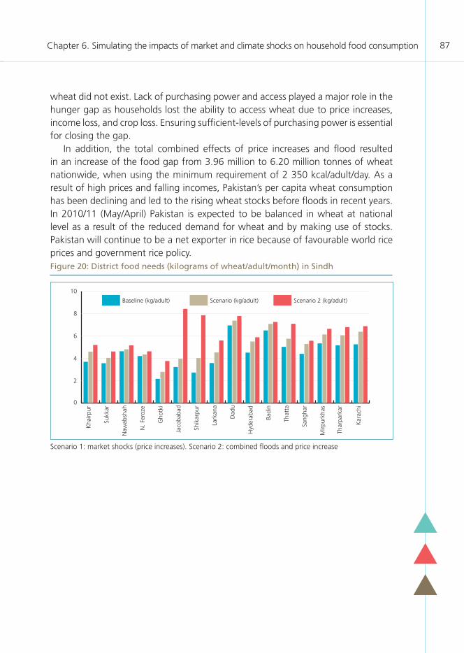
Chapter 6. Simulating the impacts of market and climate shocks on household food consumption 87
wheat did not exist. Lack of purchasing power and access played a major role in the hunger gap as households lost the ability to access wheat due to price increases, income loss, and crop loss. Ensuring sufficient-levels of purchasing power is essential for closing the gap.
In addition, the total combined effects of price increases and flood resulted in an increase of the food gap from 3.96 million to 6.20 million tonnes of wheat nationwide, when using the minimum requirement of 2 350 kcal/adult/day. As a result of high prices and falling incomes, Pakistan’s per capita wheat consumption has been declining and led to the rising wheat stocks before floods in recent years. In 2010/11 (May/April) Pakistan is expected to be balanced in wheat at national level as a result of the reduced demand for wheat and by making use of stocks. Pakistan will continue to be a net exporter in rice because of favourable world rice prices and government rice policy.Figure 20: District food needs (kilograms of wheat/adult/month) in Sindh
Scenario 1: market shocks (price increases). Scenario 2: combined floods and price increase
0
2
4
6
8
10
Scenario 2 (kg/adult)Scenario (kg/adult)Baseline (kg/adult)
Kar
achi
Thar
park
ar
Mirp
urkh
as
Sang
har
That
ta
Badi
n
Hyd
erab
ad
Dad
u
Lark
ana
Shik
arpu
r
Jaco
baba
d
Gho
tki
N. F
eroz
e
Naw
absh
ah
Sukk
ar
Kha
irpur


7. Conclusions
89
The Pakistan case study shows that price increases and floods had a negative impact on household food security. This assessment report provides valuable information for monitoring, preparing and responding to future shocks, in order to minimize the impacts on undernourishment. The price transmission and crop production analyses highlighted the trajectory of market and climate shocks by exposing the key markers to price and production changes.
In order to estimate the impacts of a market shock in the simulation model, the price transmission relationships where estimated for wheat and rice prices. The key wheat markets that are most sensitive to international price shocks and are therefore important for monitoring are Hyderabad and Peshawar. In the case of domestic price shocks, Karachi, Rawalpindi, Multan and Peshawar are the leading wheat markets that need monitoring. The IRRI rice markets that are key for monitoring domestic price changes are Islamabad, Karachi, Lahore, Quetta, Rawalpindi, and Multan. Multan, Sukkur, Peshawar, Rawalpindi, and Quetta are the leading IRRI rice markets for international price shocks. Among the basmati rice markets, the Peshawar, Hyderabad and Multan are domestic price-setting markets, while Hyderabad is the only market to monitor for international price shocks. Monitoring of the identified leading markets can provide early warning information on the first signs of a price shock.
Likewise, the results of the relationships between baseline wheat production and natural disasters (floods and droughts) can provide early warning information on production areas most likely to show the first signs of a climate shock in the Pakistan context. Wheat yield in the four main provinces in Pakistan are receptive to weather shocks, but the most at risk wheat producing areas for monitoring weather shocks are Punjab and KPK.
The results of the Household vulnerability and food security module show that a household’s relationship with the agricultural sector in sustaining its livelihood plays a large role in the type of shock and the extent to which it is affected. Livelihood groups who depend on the agricultural sector have a more distributed share of income sources among crop income, agricultural wage income and non-agricultural income, and would be impacted by both market and climate shocks. Livelihoods groups that are less directly dependent on the agricultural sector and whose main

Food price volatility and natural hazards in Pakistan90
incomes are sourced from non-agricultural wage income, are likely to be most impacted by market shocks. These assumptions are further supported by the results of the simulation model.
In the case of price increases, on the provincial level Sindh and Baluchistan were the two most affected provinces. Households of employers, paid employees and pastoralists in rural areas and service sector and industrial based households in urban areas were the most affected livelihood groups. The main income source of employers, paid employees, service sector and industrial sector livelihoods is non-agricultural wage income, which accounts for over 80 percent of income on average in all four of the main provinces in Pakistan. Among the various livelihood groups, paid employees and pastoralists are most sensitive to the impact of market shocks on undernourishment.
In the case of floods, the households that are most affected are sharecroppers and owner cultivators. Among the livelihood groups, the share of income sources is well distributed among the three income sources mentioned above, for all groups except paid employees. Sharecroppers are the most at risk to increased undernourishment during the occurrence of flood shocks. Among the four provinces, over 80 percent of sharecroppers’ income is derived from the agricultural sector. Among the provinces Sindh was most affected by floods in the simulation model and sharecroppers in Sindh derive roughly 88 percent of their income from the agricultural sector. Furthermore, in the situation of the combined impacts of market and flood shocks, the most affected livelihood groups are sharecroppers and paid employees.
In total, it is estimated that an additional 18 million people became undernourished because of price increases and the severe flood of August 2010, increasing the total number of undernourished population from the baseline situation of 77.6 million people in 2005/2006 to 95.7 million people. On average, the undernourished population is about 603 kcal per day below the minimum requirement of 2 350 kcal/adult/day and about 6 million tonnes per annum of wheat is necessary to meet their requirements. Increasing purchasing power is essential for the undernourished to obtain access to wheat. However, based on the wheat balance, it is apparent that both national reserves and private imports alone are insufficient to meet the gap.
In conclusion, the findings of the Pakistan case study identified the transmission channels of market and climate shocks to household food security. The impacts of the shocks were measured through the Percentage of people consuming less than the DECR, the number of people affected, the Depth of Hunger, and the food needs to meet their post-crisis food requirements. As such, the simulation results can be used for shock impact mitigation responses. Further research can be carried out to simulate the potential impacts of crop forecast and future international price changes on household food security in Pakistan, building on the relationships established in this case study between international prices and domestic prices and between rainfall and production.

References
91
Barrett, C.B. 1996. Markets Analysis Methods: Are Our Enriched Toolkits Well Suited to Enlivened Markets? American Journal of Agricultural Economics, 78: 825-829.
CNN Wire Staff. 18 January 2011. Major Earthquake Strikes Southwestern Pakistan. CNN (available at http://articles.cnn.com/2011-01-18/world/pakistan.quake_1_major-damage-magnitudes-quake?_s=PM:WORLD)
Deaton, A.S. & Muellbauer, J. 1980. An Almost Ideal Demand System. American Economic Review, 70: 213-326.
EM-DAT. 2010. The OFDA/CRED International Disaster Database – www.emdat.be – Université Catholique de Louvain – Brussels – Belgium.
FAO. 2008. Deriving food security information from national household budget surveys: Experiences, Achievements, Challenges (available at ftp://ftp.fao.org/docrep/fao/011/i0430e/i0430e.pdf).
FAO. 2009. The State of Food Insecurity in the World: Economic crises – impacts and lessons learned. Economic and Social Development Department, FAO (available at ftp://ftp.fao.org/docrep/fao/012/i0876e/i0876e.pdf).
FAO. 2010. Measuring dietary energy deficiency and the impact of food price variations at the household level. Anriquez, G., Karfakis, P., Daidone, S. & Mane, E. ESA Working paper No. 10-02. Agricultural Development Economics Division, FAO (available at http://www.fao.org/docrep/012/al299e/al299e00.pdf).
FAO, UNDP, UNESCO, UNICEF, WFP & WHO. 2008. High Food Prices in Pakistan: Impact Assessment and the Way Forward. The UN Inter Agency Assessment Mission (available at http://www.fao.org/giews/english/otherpub/PakistanImpactAssessment.pdf).

Food price volatility and natural hazards in Pakistan92
Government of Pakistan. 2001. Pakistan Integrated Household Survey: Poverty in the 1990s. (available at http://siteresources.worldbank.org/PAKISTANEXTN/Resources/pdf-Files-in-Events/Poverty+Paper.pdf)
Government of Pakistan. 2010. Pakistan Economic Survey 2009-2010. Finance Division (available at http://www.finance.gov.pk/survey_0910.html).
Government of Pakistan. 2011. Federal Bureau of Statistics (available at http://www.statpak.gov.pk/fbs/).
Granger, C.W.J. & Newbold, P. 1974. Spurious Regressions in Econometrics. Journal of Econometrics, 2: 111–120.
Gupta, S. & Mueller, R.A.E. 1982. Analyzing the Pricing Efficiency in Spatial Markets: Concept and Application. European Review of Agricultural Economics, 9: 301–312.
Jensen, H.H. & Manrique, J. 1996. Disaggregated Welfare Effects of Agricultural Price Polices in Urban Indonesia. Working Paper 96-WP 173, CARD/ISU. Centre for Agricultural and Rural Development, Iowa State University (available at http://www.card.iastate.edu/publications/dbs/pdffiles/96wp173.pdf).
Kasteridis, P., Yen, S. T. & Fang, C. 2011. Bayesian Estimation of a Censored Linear Almost Ideal Demand System: Food Demand in Pakistan, American Journal of Agricultural Economics, 93 (5): 1374-1390.
Kuroda, Y. & Yotopoulos, P. A. 1978. A Microeconomic Analysis of Production Behavior of the Farm Household in Japan: A Profit Function Approach. The Economic Review (Japan), 29: 115-129.
Maplecroft. 2010. BRICs and N11 countries top Maplecroft’s natural disaster risk ranking (available at http://www.maplecroft.com/about/news/natural_disasters.html).
Raza, A. & Carroll, J. 2010. Pakistan Grain and Feed Annual Report. USDA Foreign Agricultural Service.
Singh, I., Squire, L. & Strauss, J. 1986. Agricultural Household Models—Extensions, Applications and Policy. Baltimore. The Johns Hopkins University Press.

References 93
Smith, L. C., Alderman, H. & Aduayom, D. 2006. Food Insecurity in Sub-Saharan Africa: New Estimates from Household Expenditure Surveys. Research Report 146. International Food Policy Research Institute.
Timmer, P., & Aldermand, H. 1979. Estimating Consumption Parameters for Food Policy Analysis. American Journal of Agricultural Economics, 61: 982-987.
Ulimwengu, J.M. & Ramadan, R. 2009. How Does Food Price Increase Affect Ugandan Households? An Augmented Multimarket Approach. International Food Policy Research Institute.
UNISIC. 2011. Classification: International Standards Industrial Classification of all Economic Activities (ISIC). (available at http://unstats.un.org/unsd/cr/registry/regcst.asp?Cl=27)
UNISDR. 2009. Terminology: Basic terms of disaster risk reduction. United Nations International Strategy for Disaster Reduction (available at http://www.unisdr.org/eng/library/lib-terminology-eng%20home.htm)
WFP. 2010. Food Security and Market Assessment in Crisis Areas of NWFP and FATA, Pakistan. World Food Programme (available at http://home.wfp.org/stellent/groups/public/documents/ena/wfp221262.pdf).
WTO. 2002. Pakistan: January 2002. Trade Reviews Press Release. World Trade Organization. (Available at http://www.wto.org/english/tratop_e/tpr_e/tp185_e.htm).
WTO. 2008. Trade Policy Review: Pakistan. World Trade Organization (available at http://www.wto.org/english/tratop_e/tpr_e/tp293_e.htm).
World Bank. 2010a. Migration and Remittances Factbook 2011 (available at http://web.worldbank.org/WBSITE/EXTERNAL/TOPICS/0,,contentMDK:21924020 ~pagePK:5105988~piPK:360975~theSitePK:214971,00.html).
World Bank. 2010b. World Development Indicators (http://data.worldbank.org/data-catatog/world-development-indicators).S/0,,contentMDK:21924020~pagePK:5105988~piPK:360975~theSitePK:214971,00.html).

Appendix 1: Tables and figures on market integration analysis (Chapter 3), vulnerability analysis (Chapter 4) and household food security profiling (Chapter 5)

App
endi
x 1
96
Emp = employees; Wage ag = agricultural wages Wage no ag = non-agricultural wages Wage pub = public wages
Source: Compiled by the authors
Table A1.1: Example tables of income sources and disaggregated crop Income
Crop Livestock Wage ag. Wage no
ag.Wage pup Remit Other
By source and livelihood ...............................................(%) ...............................................
Employer (<10 empl.) 1.8 2.9 3.7 53.3 25.9 5.8 6.6
Employer (>10 empl.) 1.1 0.5 0.9 79.9 8.2 4.9 4.4
Self-employed 4.1 5.2 5.3 56.0 21.0 3.3 5.1
Paid employee 4.7 3.8 16.1 45.8 23.7 2.3 3.5
Unpaid family worker 18.0 10.0 29.6 17.0 6.7 13.2 5.4
Owner cultivator 30.7 11.8 43.3 5.5 2.8 4.4 1.5
Share cropper 32.2 11.1 43.8 7.3 2.2 2.8 0.6
Contract cultivator 37.1 12.5 39.3 5.2 1.6 3.5 0.7
Livestock only 1.1 30.6 29.7 7.5 2.2 6.4 22.4
RURAL PAKISTAN: PER CAPITA MONTHLY INCOME (%) BY SOURCE AND LIVELIHOOD
Source: Compiled by the authors
Wheat Rice Maize Cotton Sugarcane Pulse Fruits
By crop ...............................................(%) ...............................................
Employer (<10 empl.) 69.9 9.7 10.2 10.3 0.0 0.0 0.0
Employer (>10 empl.) 94.2 0.0 3.3 0.0 0.0 0.0 2.5
Self-employed 46.4 13.0 2.3 29.4 2.3 1.5 5.0
Paid employee 39.3 19.1 5.6 16.6 5.1 0.4 13.9
Unpaid family worker 41.6 9.2 1.7 31.1 14.4 1.8 0.2
Owner cultivator 44.1 16.5 2.1 21.9 7.6 1.0 6.8
Share cropper 41.8 19.3 1.6 27.5 7.8 1.4 0.7
Contract cultivator 43.8 14.3 7.1 23.9 10.2 0.3 0.4
Livestock only 35.2 23.5 12.0 27.7 0.0 1.4 0.2
RURAL PAKISTAN: % OF PER CAPITA CROP INCOME

Appendix 1
97
Tab
le A
1.2:
Co
effi
cien
ts o
f co
rrel
atio
n b
etw
een
wh
eat
pri
ces
(Jan
uar
y 19
93-M
arch
200
9)
Fa
isal
abad
Guj
ranw
ala
Hyd
erab
adH
yder
abad
W
Kara
chi
Laho
re
WLa
hore
M
ulta
n W
Mul
tan
Pesh
awar
W
Pesh
awar
Ra
wal
pind
iRa
wal
pind
i W
Sarg
hoda
Sial
kot
Sukk
ur
WSu
kkur
Fais
alab
ad1.
00
Gu
jran
wal
a0.
431.
00
Hyd
erab
ad0.
200.
241.
00
Hyd
erab
ad W
0.31
0.24
0.20
1.00
Kar
ach
i0.
310.
470.
160.
161.
00
Lah
ore
W0.
240.
260.
240.
650.
061.
00
Lah
ore
0.
630.
630.
230.
290.
420.
231.
00
Mu
ltan
W0.
100.
070.
100.
260.
090.
250.
131.
00
Mu
ltan
0.
710.
610.
220.
350.
370.
310.
680.
061.
00
Pesh
awar
W0.
310.
100.
250.
58-0
.01
0.70
0.29
0.30
0.24
1.00
Pesh
awar
0.
480.
270.
130.
270.
500.
090.
460.
130.
440.
181.
00
Raw
alp
ind
i0.
640.
490.
240.
280.
420.
180.
690.
080.
610.
280.
491.
00
Raw
alp
ind
i W0.
170.
200.
230.
570.
030.
770.
230.
210.
270.
570.
110.
201.
00
Sarg
ho
da
0.81
0.59
0.23
0.33
0.39
0.27
0.70
0.09
0.73
0.30
0.55
0.61
0.14
1.00
Sial
kot
0.64
0.66
0.33
0.24
0.48
0.23
0.74
0.05
0.62
0.19
0.49
0.66
0.21
0.77
1.00
Sukk
ur
W-0
.01
0.01
0.07
0.03
0.03
0.06
-0.0
50.
54-0
.02
0.06
-0.0
8-0
.05
0.18
-0.0
10.
061.
00
Sukk
ur
0.50
0.57
0.30
0.24
0.64
0.14
0.56
0.00
0.53
0.02
0.49
0.48
0.12
0.62
0.72
0.05
1.00
“W
” in
dica
tes
who
lesa
le; f
or e
xam
ple,
Lah
ore
= L
ahor
e re
tail
pric
e; L
ahor
e W
= L
ahor
e w
hole
sale
pric
e.Th
e 10
% h
ighe
st c
oeffi
cien
ts a
re s
how
n in
red
and
the
low
est
10%
coe
ffici
ents
in g
reen
.
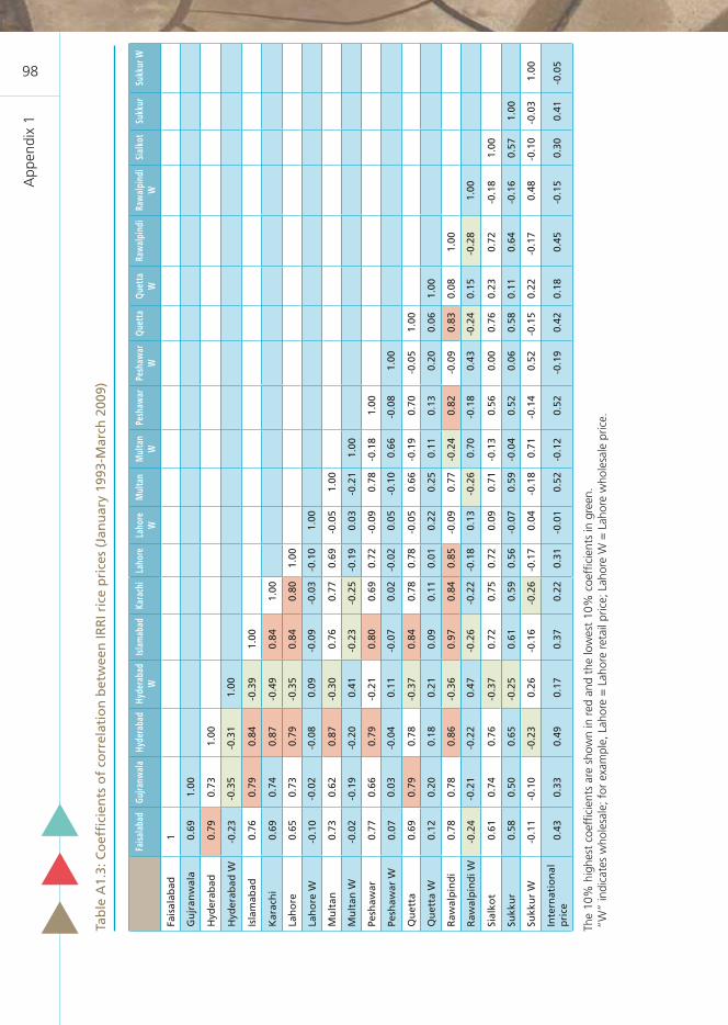
App
endi
x 1
98
Tab
le A
1.3:
Co
effi
cien
ts o
f co
rrel
atio
n b
etw
een
IRR
I ric
e p
rice
s (J
anu
ary
1993
-Mar
ch 2
009)
The
10%
hig
hest
coe
ffici
ents
are
sho
wn
in r
ed a
nd t
he lo
wes
t 10
% c
oeffi
cien
ts in
gre
en.
“W
” in
dica
tes
who
lesa
le; f
or e
xam
ple,
Lah
ore
= L
ahor
e re
tail
pric
e; L
ahor
e W
= L
ahor
e w
hole
sale
pric
e.
Fa
isala
bad
Gujra
nwal
aHy
dera
bad
Hyde
raba
d W
Islam
abad
Kara
chi
Laho
reLa
hore
W
Mul
tan
Mul
tan
WPe
shaw
arPe
shaw
ar
WQu
etta
Quet
ta
WRa
wal
pind
iRa
wal
pind
i W
Sial
kot
Sukk
urSu
kkur
W
Fais
alab
ad1
Gu
jran
wal
a0.
691.
00
Hyd
erab
ad0.
790.
731.
00
Hyd
erab
ad W
-0.2
3-0
.35
-0.3
11.
00
Isla
mab
ad0.
760.
790.
84-0
.39
1.00
Kar
ach
i0.
690.
740.
87-0
.49
0.84
1.00
Lah
ore
0.65
0.73
0.79
-0.3
50.
840.
801.
00
Lah
ore
W-0
.10
-0.0
2-0
.08
0.09
-0.0
9-0
.03
-0.1
01.
00
Mu
ltan
0.73
0.62
0.87
-0.3
00.
760.
770.
69-0
.05
1.00
Mu
ltan
W-0
.02
-0.1
9-0
.20
0.41
-0.2
3-0
.25
-0.1
90.
03-0
.21
1.00
Pesh
awar
0.77
0.66
0.79
-0.2
10.
800.
690.
72-0
.09
0.78
-0.1
81.
00
Pesh
awar
W0.
070.
03-0
.04
0.11
-0.0
70.
02-0
.02
0.05
-0.1
00.
66-0
.08
1.00
Qu
etta
0.69
0.79
0.78
-0.3
70.
840.
780.
78-0
.05
0.66
-0.1
90.
70-0
.05
1.00
Qu
etta
W0.
120.
200.
180.
210.
090.
110.
010.
220.
250.
110.
130.
200.
061.
00
Raw
alp
ind
i0.
780.
780.
86-0
.36
0.97
0.84
0.85
-0.0
90.
77-0
.24
0.82
-0.0
90.
830.
081.
00
Raw
alp
ind
i W-0
.24
-0.2
1-0
.22
0.47
-0.2
6-0
.22
-0.1
80.
13-0
.26
0.70
-0.1
80.
43-0
.24
0.15
-0.2
81.
00
Sial
kot
0.61
0.74
0.76
-0.3
70.
720.
750.
720.
090.
71-0
.13
0.56
0.00
0.76
0.23
0.72
-0.1
81.
00
Sukk
ur
0.58
0.50
0.65
-0.2
50.
610.
590.
56-0
.07
0.59
-0.0
40.
520.
060.
580.
110.
64-0
.16
0.57
1.00
Sukk
ur
W-0
.11
-0.1
0-0
.23
0.26
-0.1
6-0
.26
-0.1
70.
04-0
.18
0.71
-0.1
40.
52-0
.15
0.22
-0.1
70.
48-0
.10
-0.0
31.
00
Inte
rnat
ion
al
pri
ce0.
430.
330.
490.
170.
370.
220.
31-0
.01
0.52
-0.1
20.
52-0
.19
0.42
0.18
0.45
-0.1
50.
300.
41-0
.05
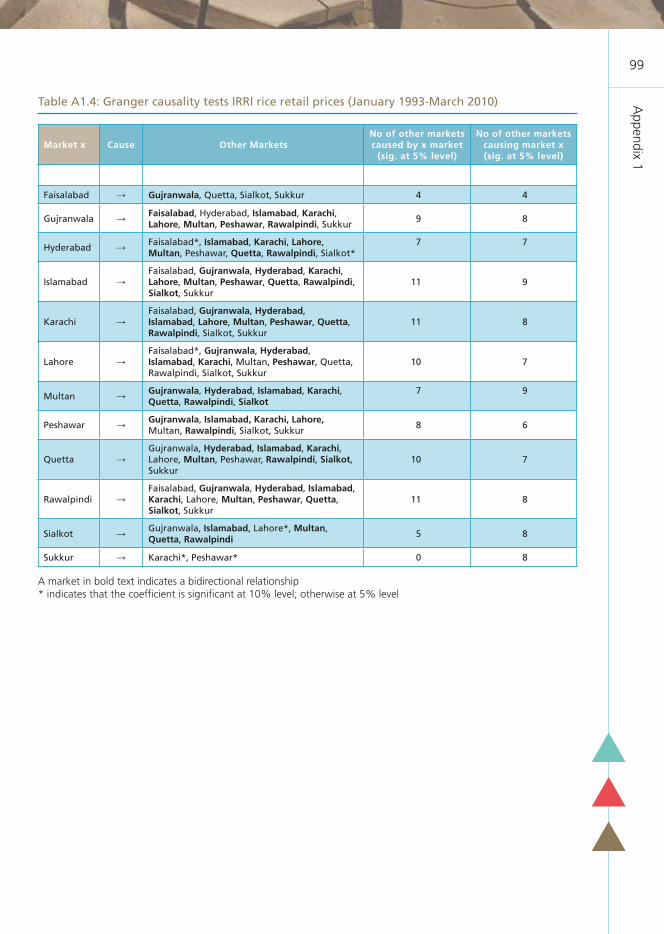
Appendix 1
99
Table A1.4: Granger causality tests IRRI rice retail prices (January 1993-March 2010)
Market x Cause Other Markets No of other markets caused by x market
(sig. at 5% level)
No of other markets causing market x (sig. at 5% level)
Faisalabad Gujranwala, Quetta, Sialkot, Sukkur 4 4
GujranwalaFaisalabad, Hyderabad, Islamabad, Karachi, Lahore, Multan, Peshawar, Rawalpindi, Sukkur
9 8
HyderabadFaisalabad*, Islamabad, Karachi, Lahore, Multan, Peshawar, Quetta, Rawalpindi, Sialkot*
7 7
IslamabadFaisalabad, Gujranwala, Hyderabad, Karachi, Lahore, Multan, Peshawar, Quetta, Rawalpindi, Sialkot, Sukkur
11 9
KarachiFaisalabad, Gujranwala, Hyderabad, Islamabad, Lahore, Multan, Peshawar, Quetta, Rawalpindi, Sialkot, Sukkur
11 8
LahoreFaisalabad*, Gujranwala, Hyderabad, Islamabad, Karachi, Multan, Peshawar, Quetta, Rawalpindi, Sialkot, Sukkur
10 7
MultanGujranwala, Hyderabad, Islamabad, Karachi, Quetta, Rawalpindi, Sialkot
7 9
PeshawarGujranwala, Islamabad, Karachi, Lahore, Multan, Rawalpindi, Sialkot, Sukkur
8 6
QuettaGujranwala, Hyderabad, Islamabad, Karachi, Lahore, Multan, Peshawar, Rawalpindi, Sialkot, Sukkur
10 7
RawalpindiFaisalabad, Gujranwala, Hyderabad, Islamabad, Karachi, Lahore, Multan, Peshawar, Quetta, Sialkot, Sukkur
11 8
SialkotGujranwala, Islamabad, Lahore*, Multan, Quetta, Rawalpindi
5 8
Sukkur Karachi*, Peshawar* 0 8
A market in bold text indicates a bidirectional relationship * indicates that the coefficient is significant at 10% level; otherwise at 5% level

App
endi
x 1
100
Table A1.5: Granger causality tests (IRRI rice wholesale prices (January 1993-March 2010)
Markets Cause #of times that a market x causes another market
# of times that a market x is caused by
another market
Hyderabad Lahore, Quetta*, Sukkur 2 4
LahoreMultan, Peshawar, Quetta, Rawalpindi, Sukkur
5 4
MultanHyderabad, Lahore*, Peshawar, Quetta, Rawalpindi, Sukkur
5 4
PeshawarHyderabad*, Lahore, Multan, Quetta, Rawalpindi, Sukkur
5 5
QuettaHyderabad, Lahore, Multan, Peshawar, Rawalpindi
5 3
RawalpindiHyderabad, Lahore, Multan, Peshawar, Sukkur
5 5
SukkurHyderabad, Lahore, Multan, Peshawar, Rawalpindi
5 5
A market in bold text indicates a bidirectional relationship * indicates that the coefficient is significant at 10% level; otherwise at 5% level

Appendix 1
101
Table A1.6: Co-integration and error correction model IRRI Rice
P1t P2tLong-run
relationship?Short-run
adjustmentP1t P2t
Long-run relationship?
Short-run adjustment
Lahore Hyderabad Yes 0.35 Rawalpindi Hyderabad Yes 0.68
Lahore Multan Yes 0.34 Rawalpindi Lahore Yes 0.44
Lahore Peshawar Yes 0.4 Rawalpindi Multan Yes 0.56
Lahore Rawalpindi Yes 0.46 Rawalpindi Peshawar Yes 0.59
Lahore Quetta Yes 0.46 Rawalpindi Quetta Yes 0.64
Lahore Sukkur Yes 0.31 Rawalpindi Sukkur Yes 0.48
Multan Hyderabad Yes 0.77 Quetta Hyderabad Yes 0.38
Multan Lahore Yes 0.41 Quetta Lahore Yes 0.27
Multan Peshawar Yes 0.82 Quetta Multan Yes 0.29
Multan Rawalpindi Yes 0.81 Quetta Peshawar Yes 0.34
Multan Quetta Yes 0.73 Quetta Rawalpindi Yes 0.32
Multan Sukkur Yes 0.69 Quetta Sukkur Yes 0.3
Peshawar Hyderabad No Sukkur Hyderabad Yes 0.6
Peshawar Lahore Yes 0.28 Sukkur Lahore Yes 0.35
Peshawar Multan Yes 0.48 Sukkur Multan Yes 0.6
Peshawar Rawalpindi Yes 0.5 Sukkur Peshawar Yes 0.64
Peshawar Quetta Yes 0.48 Sukkur Rawalpindi Yes 0.59
Peshawar Sukkur Yes 0.43
Hyderabad Lahore Yes 0.17
Hyderabad Multan Yes 0.28
Hyderabad Peshawar No
Hyderabad Rawalpindi yes 0.33
Hyderabad Quetta Yes 0.3
Hyderabad Sukkur Yes 0.24
All the coefficients are significant at 5% level

App
endi
x 1
102
Fa
isala
bad
Gujra
nwal
aHy
dera
bad
Hyde
raba
d W
Islam
abad
Kara
chi
Laho
reLa
hore
WM
ulta
nM
ulta
n W
Pesh
awar
Pesh
awar
W
Wor
ld
price
Quet
taRa
wal
pind
iRa
wal
pind
i W
Sial
kot
Sukk
ur
Fais
alab
ad1
Gu
jran
wal
a0.
621.
00
Hyd
erab
ad0.
680.
571.
00
Hyd
erab
ad W
0.01
0.07
0.06
1.00
Isla
mab
ad0.
710.
690.
710.
031.
00
Kar
ach
i0.
590.
570.
76-0
.08
0.71
1.00
Lah
ore
0.69
0.73
0.74
-0.0
50.
790.
731.
00
Lah
ore
W0.
06-0
.03
-0.0
10.
06-0
.04
-0.0
4-0
.02
1.00
Mu
ltan
0.57
0.56
0.53
0.05
0.68
0.50
0.62
-0.0
21.
00
Mu
ltan
W0.
050.
040.
000.
470.
000.
030.
030.
33-0
.01
1.00
Pesh
awar
0.64
0.58
0.77
0.11
0.77
0.69
0.68
0.04
0.55
0.02
1.00
Pesh
awar
W0.
170.
150.
02-0
.02
0.06
0.04
0.04
0.22
0.00
0.12
0.14
1.00
Wo
rld
pri
ce0.
140.
310.
190.
060.
250.
200.
23-0
.12
0.26
-0.0
20.
39-0
.11
1.00
Qu
etta
0.36
0.48
0.59
0.05
0.56
0.48
0.51
0.08
0.34
-0.0
20.
53-0
.15
0.24
1.00
Raw
alp
ind
i0.
600.
600.
600.
000.
780.
570.
67-0
.02
0.56
0.01
0.63
0.09
0.17
0.44
1.00
Rw
alp
ind
i W0.
040.
04-0
.03
0.02
0.07
0.09
0.02
0.31
0.04
0.41
0.06
0.35
-0.0
40.
050.
051.
00
Sial
kot
0.70
0.79
0.70
-0.0
50.
740.
650.
790.
020.
570.
040.
640.
230.
150.
490.
670.
051.
00
Sukk
ur0.
400.
380.
530.
050.
560.
380.
49-0
.03
0.42
0.00
0.49
0.01
0.20
0.47
0.42
-0.0
20.
441.
00
Tab
le A
1.7:
Co
effi
cien
ts o
f co
rrel
atio
n b
etw
een
Bas
mat
i ric
e p
rice
s (J
anu
ary
1993
-Mar
ch 2
009)
The
10%
hig
hest
coe
ffici
ents
are
sho
wn
in r
ed a
nd t
he lo
wes
t 10
% c
oeffi
cien
ts in
gre
en.
“W
” in
dica
tes
who
lesa
le; f
or e
xam
ple,
Lah
ore
= L
ahor
e re
tail
pric
e; L
ahor
e W
= L
ahor
e w
hole
sale
pric
e.

Appendix 1
103
Table A1.8: Granger causality tests - Basmati rice retail prices (January 1993-March 2010)
A market in bold text indicates a bidirectional relationship All the coefficients are significant at 5% level
Markets Cause
No. of times that a market x Granger-
causes another market
No. of times that a market x is Granger-caused by another
market
Faisalabad Multan 1 1
Gujranwala Hyderabad, Karachi, Lahore 3 3
Hyderabad / 0 2
Islamabad / 0 1
Karachi Faisalabad 1 4
Lahore Gujranwala 1 2
Multan Karachi, Peshawar 2 2
PeshawarGujranwala, Hyderabad,
Islamabad, Karachi, Lahore,Multan, Rawalpindi
7 1
Quetta Gujranwala, Sialkot 2 0
Rawalpindi / 0 1
Sialkot Karachi 1 1
Sukkur / 0 0
Table A1.9 Basmati rice granger causality tests - wholesale prices (January 1993-March 2010)
Markets Cause
No. of times that a market x Granger-
causes another market
No. of times that a market x is Granger-caused by another
market
Hyderabad Multan 1 1
Lahore 0 0
Multan Hyderabad 1 1
Peshawar 0 0
Rawalpindi 0 0
All the coefficients are significant at 5% level
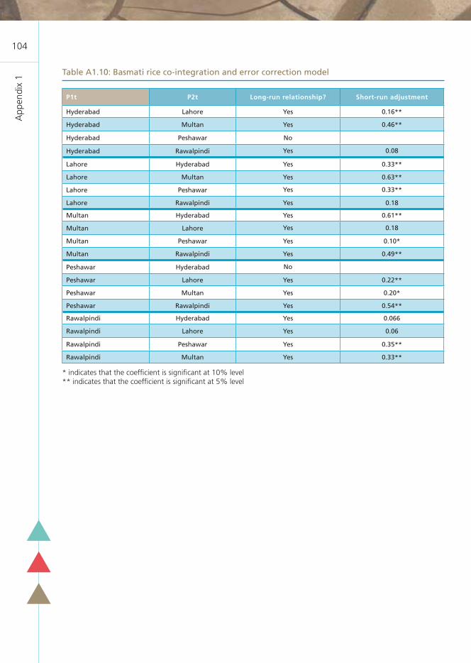
App
endi
x 1
104
Table A1.10: Basmati rice co-integration and error correction model
P1t P2t Long-run relationship? Short-run adjustment
Hyderabad Lahore Yes 0.16**
Hyderabad Multan Yes 0.46**
Hyderabad Peshawar No
Hyderabad Rawalpindi Yes 0.08
Lahore Hyderabad Yes 0.33**
Lahore Multan Yes 0.63**
Lahore Peshawar Yes 0.33**
Lahore Rawalpindi Yes 0.18
Multan Hyderabad Yes 0.61**
Multan Lahore Yes 0.18
Multan Peshawar Yes 0.10*
Multan Rawalpindi Yes 0.49**
Peshawar Hyderabad No
Peshawar Lahore Yes 0.22**
Peshawar Multan Yes 0.20*
Peshawar Rawalpindi Yes 0.54**
Rawalpindi Hyderabad Yes 0.066
Rawalpindi Lahore Yes 0.06
Rawalpindi Peshawar Yes 0.35**
Rawalpindi Multan Yes 0.33**
* indicates that the coefficient is significant at 10% level** indicates that the coefficient is significant at 5% level

Appendix 1
105
Table A1.11: Household vulnerability profiling: Urban and rural demographics
LivelihoodNo. of
householdsAge of HH
head
% Female headed
HHsHH size
% HH dependency
ratio
No. age 14 or under
No. age 15-64 yr
No. age 65 or over
LIVELIHOODS AND DEMOGRAPHICS IN RURAL AREAS BY PROVINCE IN PAKISTAN
PUNJAB
Employer 620 44 1.1 8 46.60 0.00 0.00 0.00
Paid employee 1 147 43 2.8 7 48.43 0.00 0.00 0.00
Unpaid family worker 35 56 31.2 8 47.35 0.00 0.00 0.00
Owner cultivator 951 50 1.6 9 42.92 0.00 0.00 0.00
Sharecropper 105 51 1.9 9 43.97 0.00 0.00 0.00
Contract cultivator 165 46 0.0 8 46.33 0.00 0.00 0.00
Livestock only 178 48 12.5 8 49.52 0.00 0.00 0.00
SINDH
Employer 159 43 1.3 9 46.37 0.00 0.00 0.00
Paid employee 1 003 40 0.4 8 45.95 0.00 0.00 0.00
Unpaid family worker 6 30 9.4 15 53.79 0.00 0.00 0.00
Owner cultivator 279 45 0.0 10 46.13 0.00 0.00 0.00
Sharecropper 400 44 0.0 9 50.19 0.00 0.00 0.00
Contract cultivator 14 40 0.0 8 48.51 0.00 0.00 0.00
Livestock only 49 44 1.1 9 48.77 0.00 0.00 0.00
KPK
Employer 328 45 1.1 11 47.48 0.00 0.00 0.00
Paid employee 562 43 1.4 10 49.25 0.00 0.00 0.00
Unpaid family worker 21 55 21.8 11 51.10 0.00 0.00 0.00
Owner cultivator 408 50 6.2 12 48.17 0.00 0.00 0.00
Sharecropper 100 50 1.6 11 48.15 0.00 0.00 0.00
Contract cultivator 35 52 11.1 11 51.14 0.00 0.00 0.00
Livestock only 33 46 9.4 8 52.51 0.00 0.00 0.00
BALUCHISTAN
Employer 117 45 0.3 9 50.64 0.00 0.00 0.00
Paid employee 610 42 0.0 9 48.68 0.00 0.00 0.00
Unpaid family worker 1 48 0.0 9 77.78 0.00 0.00 0.00
Owner cultivator 278 48 0.0 9 43.49 0.00 0.00 0.00
Sharecropper 88 45 0.0 9 47.53 0.00 0.00 0.00
Contract cultivator 3 41 0.0 8 41.31 0.00 0.00 0.00
Livestock only 47 50 0.0 8 49.96 0.00 0.00 0.00
LIVELIHOODS AND DEMOGRAPHICS IN URBAN AREAS BY PROVINCE IN PAKISTAN
PUNJAB
Agriculture 157 51 2.4 8 39.84 0.00 0.00 0.00
Traders 604 46 0.8 8 38.80 0.00 0.00 0.00
Social & personal service 606 45 3.9 7 39.18 0.00 0.00 0.00
Service sector 277 44 0.0 7 38.69 0.00 0.00 0.00
Industrial sector 537 43 1.7 8 41.19 0.00 0.00 0.00

App
endi
x 1
106
Table A1.11: Household vulnerability profiling: Urban and rural demographics (cont.)
Note: Livelihood groups of unpaid family worker and contract cultivator in rural Baluchistan are not shown since only very small samples were available.
LivelihoodNo. of
householdsAge of HH
head
% Female headed
HHsHH size
% HH dependency
ratio
No. age 14 or under
No. age 15-64 yr
No. age 65 or over
SINDH
Agriculture 83 46 0.0 10 45.29 0.00 0.00 0.00
Traders 358 47 0.0 8 38.36 0.00 0.00 0.00
Social & personal service 376 44 1.9 9 38.56 0.00 0.00 0.00
Service sector 158 43 0.0 8 38.38 0.00 0.00 0.00
Industrial sector 434 44 0.7 8 39.36 0.00 0.00 0.00
KPK
Agriculture 52 52 0.0 10 39.57 0.00 0.00 0.00
Traders 216 46 0.3 11 45.53 0.00 0.00 0.00
Social & personal service 243 46 1.8 8 40.42 0.00 0.00 0.00
Service sector 103 43 0.0 9 45.70 0.00 0.00 0.00
Industrial sector 150 44 0.0 8 39.75 0.00 0.00 0.00
BALUCHISTAN
Agriculture 54 46 0.0 12 46.14 0.00 0.00 0.00
Traders 113 47 0.0 11 46.11 0.00 0.00 0.00
Social & personal service 238 44 0.0 9 46.02 0.00 0.00 0.00
Service sector 101 45 0.0 10 46.88 0.00 0.00 0.00
Industrial sector 100 45 0.0 10 44.17 0.00 0.00 0.00

Appendix 1
107
Table A.12: Livelihoods and per capita monthly crop income (Rs) by commodity in urban
areas of Pakistan
Wheat Rice Maize CottonSugar cane
Pulses Fruits
PUNJAB
Agriculture 556.00 126.73 402.47 546.59 57.60 14.03 340.14
Traders 10.11 0.43 0.00 22.03 0.00 0.10 0.00
Social & personal service 13.31 3.24 0.31 23.71 3.31 0.00 0.00
Service sector 30.66 42.23 0.00 0.80 0.00 0.00 0.00
Industrial sector 27.79 14.63 0.00 13.62 6.56 0.00 0.00
SINDH
Agriculture 218.06 86.58 0.00 202.65 54.68 0.00 84.67
Traders 0.29 0.00 0.00 0.29 0.00 0.00 0.00
Social & personal service 2.87 0.68 0.00 0.00 1.30 0.00 2.27
Service sector 0.00 0.00 0.00 0.00 0.00 0.00 0.00
Industrial sector 1.25 0.36 0.00 1.64 0.00 0.00 0.00
KPK
Agriculture 95.65 14.06 18.15 0.00 18.82 0.00 0.29
Traders 3.18 0.50 0.39 0.00 0.00 0.06 0.00
Social & personal service 2.77 0.89 1.02 0.00 0.00 0.30 0.25
Service sector 9.99 0.38 1.30 0.00 0.00 0.00 0.00
Industrial sector 2.02 0.00 0.83 0.00 0.00 0.00 0.00
BALUCHISTAN
Agriculture 57.67 39.78 0.00 11.16 0.00 0.80 487.24
Traders 0.35 1.04 0.00 0.00 0.00 0.00 0.00
Social & personal service 0.00 0.00 0.00 0.00 0.00 0.00 0.00
Service sector 0.00 0.00 0.00 0.00 0.00 0.00 0.00
Industrial sector 0.00 0.00 0.00 0.00 0.00 0.00 0.00

App
endi
x 1
108
Tab
leA
1.1
3: L
ivel
iho
od
s an
d p
er c
apit
a as
sets
(la
nd
in h
ecta
re a
nd
an
nu
al v
alu
e o
f liv
esto
ck in
Rs)
in r
ura
l are
as b
y p
rovi
nce
in P
akis
tan
Lan
d
Ow
ne
dLa
nd
R
en
ted
Lan
d
Sh
are
dLi
ve
sto
ck
Ow
ne
dC
att
le
Ow
ne
dB
uff
alo
O
wn
ed
Ca
me
l O
wn
ed
Sh
ee
p
Ow
ne
dG
oa
t O
wn
ed
Ho
rse
s O
wn
ed
Ass
es
Ow
ne
dM
ule
s O
wn
ed
Po
ult
ry
Ow
ne
dO
the
r Li
ve
sto
ck
Ow
ne
d
PUN
JAB
Emp
loye
r0.
030.
010.
003
196
799
2 00
818
2118
239
2814
860
Paid
em
plo
yee
0.03
0.01
0.00
3 06
889
81
848
1815
231
635
125
0
Un
pai
d f
amily
wo
rker
0.14
0.02
0.03
7 90
72
529
4 28
80
8875
80
111
017
117
Ow
ner
cu
ltiv
ato
r0.
430.
090.
0217
573
4 28
411
131
154
211
922
673
122
173
2
Shar
ecro
pp
er0.
110.
070.
3511
485
4 15
46
014
167
235
731
099
6321
0
Co
ntr
act
cult
ivat
or
0.07
0.26
0.01
13 1
943
825
8 55
70
6058
432
115
021
0
Live
sto
ck o
nly
0.02
0.01
0.00
14 1
193
467
8 04
30
902
1 53
80
151
019
0
SIN
DH
Emp
loye
r0.
050.
000.
023
379
1 50
31
131
4814
577
010
80
00
Paid
em
plo
yee
0.05
0.00
0.02
1 79
731
11
316
517
138
08
02
0
Un
pai
d f
amily
wo
rker
0.17
0.00
0.08
5 46
540
14
874
00
180
00
09
0
Ow
ner
cu
ltiv
ato
r0.
440.
000.
027
301
1 56
85
119
051
507
031
011
14
Shar
ecro
pp
er0.
020.
030.
285
472
1 43
73
489
066
429
145
05
0
Co
ntr
act
cult
ivat
or
0.05
0.29
0.03
2 84
732
72
218
00
301
00
00
0
Live
sto
ck o
nly
0.00
0.00
0.03
15 3
752
535
10 5
170
171
1 12
781
03
021
20
KPK
Emp
loye
r0.
090.
000.
001
083
511
330
1913
190
04
015
0
Paid
em
plo
yee
0.06
0.00
0.00
1 36
172
434
30
3618
821
260
231
Un
pai
d f
amily
wo
rker
0.11
0.04
0.00
51 8
2748
350
972
040
190
128
00
150
Ow
ner
cu
ltiv
ato
r0.
160.
000.
015
006
2 54
11
553
5095
581
3481
068
3
Shar
ecro
pp
er0.
060.
130.
064
898
2 65
81
431
189
4041
60
790
5530
Co
ntr
act
cult
ivat
or
0.05
0.07
0.01
5 30
12
224
2 33
70
9855
20
480
420
Live
sto
ck o
nly
0.03
0.00
0.00
10 7
382
845
5 47
10
225
1 75
345
204
010
689

Appendix 1
109
Tabl
eA 1
.13:
Liv
elih
oods
and
per
cap
ita
asse
ts (l
and
in h
ecta
re a
nd a
nnua
l val
ue o
f liv
esto
ck in
Rs)
in r
ural
are
as b
y pr
ovin
ce in
Pak
ista
n - C
ont.
Lan
d
Ow
ne
dLa
nd
R
en
ted
Lan
d
Sh
are
dLi
ve
sto
ck
Ow
ne
dC
att
le
Ow
ne
dB
uff
alo
O
wn
ed
Ca
me
l O
wn
ed
Sh
ee
p
Ow
ne
dG
oa
t O
wn
ed
Ho
rse
s O
wn
ed
Ass
es
Ow
ne
dM
ule
s O
wn
ed
Po
ult
ry
Ow
ne
dO
the
r Li
ve
sto
ck
Ow
ne
d
BA
LOC
HIS
TAN
Emp
loye
r0,
020,
010,
0263
329
510
061
4712
90
00
00
Paid
em
plo
yee
0,04
0,00
0,00
887
129
124
6094
466
010
05
0
Un
pai
d f
amily
wo
rker
0,00
0,00
0,00
1.11
10
00
01.
111
00
00
0
Ow
ner
cu
ltiv
ato
r0,
570,
000,
002
711
397
271
435
589
930
068
020
0
Shar
ecro
pp
er0,
100,
010,
424
502
1 57
31
993
017
070
525
300
60
Co
ntr
act
cult
ivat
or
0,00
0,00
0,27
0 28
80
00
028
80
00
00
Live
sto
ck o
nly
0,02
0,00
0,00
11 1
0150
128
956
95
581
4 02
356
680
130
Not
e: L
ivel
ihoo
d gr
oups
of
unpa
id f
amily
wor
ker
and
cont
ract
cul
tivat
or in
Bal
uchi
stan
are
not
sho
wn
sinc
e on
ly v
ery
smal
l sam
ples
wer
e av
aila
ble

App
endi
x 1
110
Tab
le A
1.14
: Liv
elih
oo
ds
and
per
cap
ita
asse
ts (l
and
in h
ecta
re a
nd
an
nu
al v
alu
e o
f liv
esto
ck in
Rs)
in U
rban
are
as b
y p
rovi
nce
in P
akis
tan
Lan
d
Ow
ne
dLa
nd
R
en
ted
Lan
d
Sh
are
dLi
ve
sto
ck
Ow
ne
dC
att
le
Ow
ne
dB
uff
alo
O
wn
ed
Ca
me
l O
wn
ed
Sh
ee
p
Ow
ne
dG
oa
t O
wn
ed
Ho
rse
s O
wn
ed
Ass
es
Ow
ne
dM
ule
s O
wn
ed
Pou
ltry
O
wn
ed
Oth
er
Live
sto
ck
Ow
ned
PUN
JAB
Ag
ricu
ltu
re0.
240.
090.
0113
909
3 39
99
738
563
447
136
7336
210
Trad
ers
0.00
0.01
0.00
440
6834
40
021
42
01
0
Soci
al &
per
son
al s
ervi
ce0.
010.
000.
0060
576
459
241
180
10
260
Serv
ice
sect
or
0.01
0.00
0.00
176
3712
90
07
03
00
0
Ind
ust
rial
sec
tor
0.01
0.01
0.00
647
147
464
09
220
20
30
SIN
DH
Ag
ricu
ltu
re0.
170.
010.
025
562
358
4 61
60
2244
00
440
820
Trad
ers
0.00
0.00
0.00
228
2420
10
02
00
00
0
Soci
al &
per
son
al s
ervi
ce0.
000.
000.
0011
630
690
017
00
00
0
Serv
ice
sect
or
0.00
0.00
0.00
810
600
00
00
021
0
Ind
ust
rial
sec
tor
0.00
0.00
0.00
135
2011
20
03
00
00
0
KPK
Ag
ricu
ltu
re0.
310.
010.
013
782
1 24
51
554
3925
639
043
023
70
Trad
ers
0.00
0.00
0.00
356
121
218
00
140
10
20
Soci
al &
per
son
al s
ervi
ce0.
000.
000.
0019
814
154
00
00
00
30
Serv
ice
sect
or
0.08
0.00
0.00
374
3531
90
016
00
03
0
Ind
ust
rial
sec
tor
0.01
0.00
0.00
288
129
132
00
220
10
40
BA
LOC
HIS
TAN
Ag
ricu
ltu
re0.
070.
000.
001
884
178
1 57
70
512
00
10
30
Trad
ers
0.00
0.00
0.00
148
014
70
00
00
01
0
Soci
al &
per
son
al s
ervi
ce0.
000.
000.
0042
160
00
250
00
10
Serv
ice
sect
or
0.00
0.00
0.00
7062
00
08
00
01
0
Ind
ust
rial
sec
tor
0.00
0.00
0.00
580
580
00
00
00
0

Appendix 1
111
Table A1.15: Livelihoods and per capita monthly expenditures (Rs) in rural areas by province in Pakistan
Note: Livelihood groups of unpaid family worker and contract cultivator in Baluchistan are not shown since only very small samples were available.
Livelihood Total Recreation Transport Apperal Housing Medical Education Fuel Food
PUNJAB
Employer 1 193.0 2.4 63.6 97.4 133.1 69.5 34.9 60.7 435.8
Paid employee 1 074.4 1.3 61.3 83.9 125.7 54.4 32.7 59.7 410.3
Unpaid family worker 1 049.4 2.6 75.2 96.0 105.0 33.8 18.8 69.0 326.6
Owner cultivator 1 199.7 1.2 70.5 108.3 132.7 77.0 40.4 67.2 341.1
Sharecropper 951.0 1.0 47.0 86.4 85.4 98.0 28.3 57.7 297.5
Contract cultivator 992.7 0.7 51.2 93.0 110.9 61.8 22.8 56.5 310.1
Livestock only 1 052.4 0.2 46.5 81.7 125.3 47.9 22.0 60.1 401.7
SINDH
Employer 1 179.2 5.6 79.8 82.9 167.5 57.9 26.2 43.4 452.8
Paid employee 962.4 1.5 79.5 69.1 114.2 44.6 15.1 41.8 412.3
Unpaid family worker 669.9 0.0 64.9 58.3 88.9 24.8 4.6 42.5 283.0
Owner cultivator 889.6 1.0 75.7 75.0 99.2 61.4 13.0 39.6 316.8
Sharecropper 665.6 0.2 41.3 58.9 76.6 40.7 6.1 37.3 263.0
Contract cultivator 966.1 0.0 102.9 69.8 88.8 51.8 10.8 37.8 411.7
Livestock only 1 180.4 2.0 89.8 89.9 109.1 64.0 17.2 41.4 353.3
KPK
Employer 1 270.6 1.6 60.2 87.3 107.5 93.6 52.4 76.2 481.3
Paid employee 1 148.7 1.4 57.5 75.7 97.5 69.6 56.3 89.2 466.1
Unpaid family worker 1 270.5 3.8 49.6 86.6 122.9 92.7 48.6 96.8 514.5
Owner cultivator 1 090.0 0.9 56.4 84.1 87.2 89.2 37.4 92.6 407.6
Sharecropper 838.8 0.1 32.6 72.0 62.7 80.8 23.0 63.7 326.1
Contract cultivator 739.2 0.0 26.7 66.8 50.2 42.8 16.9 70.8 348.6
Livestock only 986.9 0.0 34.4 69.0 85.4 69.0 18.5 89.4 431.2
BALOCHISTAN
Employer 1 085.3 2.4 87.9 55.1 153.2 23.2 16.5 57.1 517.1
Paid employee 943.5 2.4 73.4 52.4 109.1 20.5 12.9 55.2 480.4
Unpaid family worker 502.1 0.0 33.3 47.2 23.1 3.7 7.4 28.3 290.6
Owner cultivator 908.0 2.2 83.2 61.0 101.1 29.0 9.2 63.2 393.0
Sharecropper 716.2 1.1 68.2 59.3 75.6 32.1 4.1 46.3 302.5
Contract cultivator 934.7 0.0 93.7 46.7 133.1 18.3 6.6 40.8 420.2
Livestock only 762.3 1.4 65.7 49.2 66.3 21.2 4.4 53.7 384.3
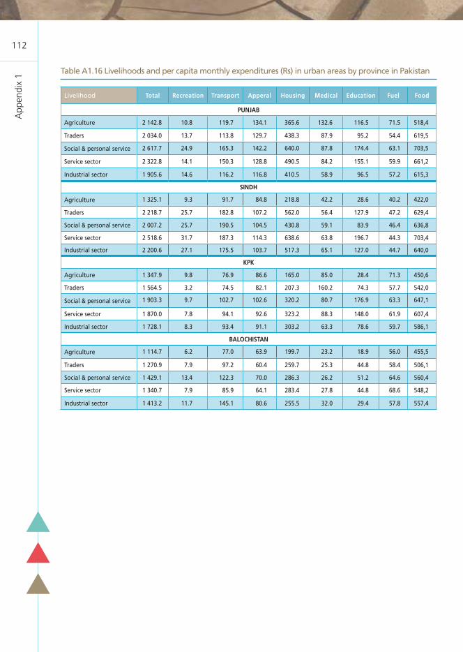
App
endi
x 1
112
Table A1.16 Livelihoods and per capita monthly expenditures (Rs) in urban areas by province in Pakistan
Livelihood Total Recreation Transport Apperal Housing Medical Education Fuel Food
PUNJAB
Agriculture 2 142.8 10.8 119.7 134.1 365.6 132.6 116.5 71.5 518,4
Traders 2 034.0 13.7 113.8 129.7 438.3 87.9 95.2 54.4 619,5
Social & personal service 2 617.7 24.9 165.3 142.2 640.0 87.8 174.4 63.1 703,5
Service sector 2 322.8 14.1 150.3 128.8 490.5 84.2 155.1 59.9 661,2
Industrial sector 1 905.6 14.6 116.2 116.8 410.5 58.9 96.5 57.2 615,3
SINDH
Agriculture 1 325.1 9.3 91.7 84.8 218.8 42.2 28.6 40.2 422,0
Traders 2 218.7 25.7 182.8 107.2 562.0 56.4 127.9 47.2 629,4
Social & personal service 2 007.2 25.7 190.5 104.5 430.8 59.1 83.9 46.4 636,8
Service sector 2 518.6 31.7 187.3 114.3 638.6 63.8 196.7 44.3 703,4
Industrial sector 2 200.6 27.1 175.5 103.7 517.3 65.1 127.0 44.7 640,0
KPK
Agriculture 1 347.9 9.8 76.9 86.6 165.0 85.0 28.4 71.3 450,6
Traders 1 564.5 3.2 74.5 82.1 207.3 160.2 74.3 57.7 542,0
Social & personal service 1 903.3 9.7 102.7 102.6 320.2 80.7 176.9 63.3 647,1
Service sector 1 870.0 7.8 94.1 92.6 323.2 88.3 148.0 61.9 607,4
Industrial sector 1 728.1 8.3 93.4 91.1 303.2 63.3 78.6 59.7 586,1
BALOCHISTAN
Agriculture 1 114.7 6.2 77.0 63.9 199.7 23.2 18.9 56.0 455,5
Traders 1 270.9 7.9 97.2 60.4 259.7 25.3 44.8 58.4 506,1
Social & personal service 1 429.1 13.4 122.3 70.0 286.3 26.2 51.2 64.6 560,4
Service sector 1 340.7 7.9 85.9 64.1 283.4 27.8 44.8 68.6 548,2
Industrial sector 1 413.2 11.7 145.1 80.6 255.5 32.0 29.4 57.8 557,4

Appendix 1
113
Table A1.17: Household vulnerability profiling: Rural caloric intake (kcal/person/day)
Note: Livelihood groups of unpaid family worker and contract cultivator in Baluchistan are not shown since only very small samples were available.
LivelihoodTotal food
Milk Meat Eggs FishFresh Fruits
Dry Fruits
Potatoes Vegetable
PUNJAB
Employer 2 318 355.5 15.8 8.4 0.8 37.6 0.7 30.9 40.6
Paid employee 2 215 322.5 13.5 7.2 0.5 29.6 0.5 30.5 42.4
Unpaid family worker 2 501 471.6 12.1 9.3 0.5 25.2 0.3 27.5 32.8
Owner cultivator 2 925 751.8 17.1 11.0 0.8 41.9 1.1 32.5 36.6
Sharecropper 2 650 492.8 13.1 7.5 0.2 27.7 1.2 31.6 32.5
Contract cultivator 2 690 568.2 15.1 10.4 0.6 34.6 0.9 31.0 39.5
Livestock only 2 625 544.9 13.3 9.3 0.1 30.3 0.7 33.5 36.2
SINDH
Employer 2 094 192.1 16.0 6.5 13.5 46.2 1.0 43.8 36.2
Paid employee 1 984 181.2 13.9 3.7 8.6 37.0 0.0 31.7 33.1
Unpaid family worker 2 145 279.7 16.3 3.5 5.3 11.5 0.0 47.4 29.7
Owner cultivator 2 380 381.2 16.0 4.6 12.7 36.6 0.0 42.1 32.0
Sharecropper 2 117 263.9 9.5 2.2 6.7 27.5 0.1 40.8 29.6
Contract cultivator 2 274 174.5 15.1 2.3 8.5 54.5 0.0 28.3 31.0
Livestock only 2 384 427.7 16.3 4.6 9.0 36.1 0.0 34.2 30.3
KPK
Employer 2 509 262.0 26.8 10.2 0.7 40.6 1.8 33.2 47.2
Paid employee 2 374 221.6 21.3 12.5 1.0 33.4 1.8 29.8 36.3
Unpaid family worker 2 598 308.4 36.8 15.2 0.0 40.8 0.0 30.8 31.6
Owner cultivator 2 685 341.6 18.7 12.7 0.2 30.0 2.4 32.0 34.7
Sharecropper 2 454 330.7 17.0 13.5 0.2 27.0 1.2 24.3 30.7
Contract cultivator 2 222 164.4 15.6 9.6 0.0 11.5 1.2 33.4 33.0
Livestock only 2 808 413.0 14.8 17.2 0.4 40.6 4.5 27.9 38.3
BALUCHISTAN
Employer 2 067 144.8 20.3 3.8 15.8 19.4 6.5 37.8 32.3
Paid employee 2 033 95.6 19.2 5.5 9.5 19.7 1.4 33.0 31.9
Unpaid family worker 1 517 78.2 0.0 8.2 0.0 32.8 0.0 53.9 28.3
Owner cultivator 2 192 164.6 22.0 6.4 9.2 22.4 3.3 34.2 40.8
Sharecropper 2 172 170.9 14.9 3.5 2.9 12.2 1.5 48.5 35.5
Contract cultivator 1 544 93.6 21.4 9.2 6.4 29.3 0.0 17.2 20.3
Livestock only 2 019 131.7 20.9 4.8 7.4 12.6 0.2 29.6 25.9

App
endi
x 1
114
Table A1.17: Household vulnerability profiling: Rural caloric intake (kcal/person/day) - Cont’d
Condiments and Spices
SugarNon-alcoholic
beverageWheat Rice
Other cereals
PulsesOils and
fatsTea and coffee
Baked and fried products
PUNJAB
48.1 194.1 0.5 855.4 80.3 6.9 9.8 254.9 6.6 6.4
46.2 194.3 0.4 848.8 75.0 4.8 10.6 250.5 6.6 2.5
40.5 169.4 0.3 1.002.3 70.2 4.3 8.5 265.2 7.6 0.7
267.5 222.5 0.7 986.1 93.0 8.4 11.3 266.2 7.6 1.4
41.4 232.1 0.4 1.008.0 80.7 6.2 11.4 259.9 8.0 0.8
48.8 222.8 0.4 959.1 88.0 7.7 9.9 254.0 6.8 0.6
49.9 774.6 0.5 937.0 81.4 10.4 11.4 254.6 7.1 2.7
SINDH
52.5 142.3 0.3 644.1 287.5 5.0 8.0 254.1 10.6 3.3
53.3 159.9 0.3 698.2 215.3 4.5 7.6 211.8 12.0 2.6
54.5 172.2 0.2 668.3 254.8 2.0 5.8 240.5 11.3 0.5
54.5 160.4 0.2 714.0 334.7 5.4 7.5 231.8 11.1 1.5
50.2 157.7 0.1 722.6 300.5 3.0 6.8 197.4 10.1 1.1
48.4 190.0 18.6 953.8 183.2 9.0 9.6 200.3 12.8 0.6
51.7 160.4 0.4 742.6 271.7 15.7 7.9 229.4 12.1 2.1
KPK
52.2 246.6 0.2 938.2 82.9 69.9 11.1 257.4 13.6 3.5
87.2 251.2 0.2 884.6 90.5 63.4 10.4 241.0 13.7 12.3
61.5 299.1 0.4 872.2 104.8 60.1 12.0 256.7 13.4 3.3
53.9 275.7 0.1 976.1 106.5 105.5 11.4 243.2 15.1 2.7
49.2 255.9 0.2 891.3 49.2 107.8 8.4 231.7 13.0 4.9
37.5 263.5 0.1 845.3 110.8 97.0 10.6 205.9 13.9 1.2
62.7 305.3 0.1 939.1 83.1 75.3 10.5 268.0 15.6 14.2
BALUCHISTAN
50.5 186.5 0.2 838.0 88.5 3.4 11.2 244.2 11.7 2.4
53.2 195.8 0.1 858.5 86.1 2.8 11.0 240.2 11.2 2.3
44.0 79.0 0.0 538.2 128.1 6.4 4.7 245.0 7.3 0.0
51.8 210.4 0.3 874.4 102.5 6.8 11.5 240.7 11.4 3.2
60.5 193.0 0.0 794.9 190.2 45.9 6.8 231.6 9.6 0.7
53.0 82.6 0.0 562.5 19.3 0.0 11.8 293.9 13.6 0.0
53.5 192.2 0.0 823.1 101.1 2.2 11.7 239.5 10.9 1.7

Appendix 1
115
Table A1.18: Household vulnerability profiling: Urban caloric intake (kcal/person/day)
LivelihoodTotal food
Milk Meat Eggs FishFresh fruits
Dry fruits
Potatoes Vegetable
PUNJAB
Agriculture 2 930 684.7 24.8 13.1 3.6 62.3 2.4 32.8 60.0
Traders 2 243 407.1 23.2 11.6 2.3 53.7 2.1 30.9 33.5
Social & personal service 2 437 432.3 27.1 15.8 2.5 60.4 2.7 33.7 38.4
Service sector 2 311 358.5 26.1 13.5 1.4 53.6 2.4 31.2 36.8
Industrial sector 2 269 365.7 23.1 11.3 2.5 48.1 1.9 31.7 38.2
SINDH
Agriculture 2 111 190.2 15.1 6.8 9.5 31.6 0.0 37.5 30.2
Traders 2 051 205.9 26.4 12.7 8.8 58.1 0.9 29.8 31.1
Social & personal service 2 073 211.5 23.8 14.1 9.8 59.4 0.9 29.9 30.1
Service sector 2 115 225.2 30.1 16.3 8.0 60.2 0.5 30.1 33.7
Industrial sector 2 063 190.6 24.4 15.7 7.5 58.3 1.1 29.8 33.3
KPK
Agriculture 2 697 368.0 24.3 13.4 2.5 39.9 3.6 32.2 38.7
Traders 2 309 255.4 25.0 9.5 1.6 40.2 1.0 27.1 34.2
Social & personal service 2 668 310.9 33.5 20.5 4.2 60.9 3.2 31.8 41.8
Service sector 2 376 212.3 30.9 13.4 1.4 55.3 3.9 28.1 39.3
Industrial sector 2 491 240.0 26.3 10.7 1.3 45.2 1.3 32.5 44.5
BALUCHISTAN
Agriculture 1 879 126.3 20.7 8.3 18.3 27.3 0.0 31.5 30.2
Traders 1 792 97.8 20.3 5.8 13.8 23.9 0.7 30.1 29.1
Social & personal service 2 016 107.1 23.5 5.5 6.9 25.7 2.0 29.5 34.8
Service sector 2 007 112.0 24.1 6.7 5.6 24.8 6.7 31.1 29.4
Industrial sector 2 039 109.0 21.1 5.4 9.6 28.9 2.6 32.1 31.7
Note: Livelihood groups of unpaid family worker and contract cultivator in Baluchistan are not shown since only very small samples were available.

App
endi
x 1
116
Table A1.18: Household vulnerability profiling: Urban caloric intake (kcal/person/day) - Cont’d
Condiments and spices
SugarNon-alcoholic
beverageWheat Rice
Other cereals
PulsesOils and
fatsTea and coffee
Baked and fried products
PUNJAB
52.7 219.6 1.5 879.8 98.3 8.9 12.7 303.7 7.5 10.6
47.7 166.8 2.4 678.6 83.6 7.6 11.1 267.1 6.2 19.6
51.2 218.0 1.6 696.5 90.8 7.4 11.7 299.0 7.5 31.8
50.8 177.0 4.1 697.8 92.2 8.2 12.4 289.8 7.6 27.6
47.5 176.6 1.1 716.3 91.1 6.9 11.2 278.5 6.8 17.9
SINDH
83.3 153.2 0.4 660.3 234.7 10.2 7.4 249.0 11.0 4.3
58.2 152.0 0.9 574.2 171.7 7.2 9.3 271.2 13.0 30.9
55.9 155.2 1.0 576.5 177.0 7.7 9.2 274.4 13.5 31.3
54.6 159.3 1.1 562.3 182.9 7.3 9.2 276.1 14.0 38.0
60.3 160.7 1.2 588.2 171.5 7.1 9.7 268.7 14.2 27.0
KPK
54.6 226.6 0.1 978.6 69.9 33.2 13.4 285.8 13.6 37.8
42.7 215.1 0.5 832.0 52.3 12.9 12.2 250.7 13.0 55.9
54.0 260.7 3.4 816.0 57.0 18.1 14.7 282.9 14.2 116.1
46.6 226.3 0.6 842.5 62.6 21.8 13.5 265.2 13.5 51.9
50.3 237.0 0.5 896.5 69.3 20.4 12.5 267.0 13.5 60.2
BALUCHISTAN
49.3 167.4 0.0 658.4 132.6 4.2 9.1 229.4 10.7 2.9
47.9 168.5 0.3 666.9 99.0 2.7 8.2 222.8 10.2 5.4
51.9 201.9 0.4 738.5 88.1 2.6 10.5 255.1 11.4 25.3
50.5 234.6 0.5 750.0 81.8 3.8 9.4 245.1 9.6 21.6
50.7 196.4 0.3 721.9 131.4 3.2 9.6 267.8 11.0 14.3

Appendix 1
117
Table A1.19: Estimated food needs: Kilograms of wheat per month/adult by district
District BaselineScenario
1Scenario
2
PUNJAB
Islamabad 3.32 3.97 4.33
Attock 4.04 4.76 4.92
Rawalpindi 2.44 2.80 2.89
Jhelum 3.58 4.09 4.43
Chakwal 3.32 4.20 4.34
Sargoda 3.74 4.93 5.29
Bhakkar 4.05 4.42 4.79
Khushab 5.29 5.91 6.18
Mianwali 2.69 3.59 4.00
Faisalabad 3.46 4.16 4.63
T.T.Singh 3.03 4.15 4.37
Jhang 3.22 3.71 4.07
Gujranwala 4.54 5.02 5.49
Gujrat 3.95 4.32 4.80
Sialkot 3.08 3.91 4.40
Hafizabad 2.44 3.49 4.06
Mandi Bahaud Din 2.09 3.11 3.90
Narowal 2.77 3.58 3.42
Lahore 4.51 5.07 5.40
Kasur 3.83 4.88 5.40
Okara 3.25 4.54 4.68
Sheikhupura 3.97 5.10 5.32
Vehari 4.43 4.49 4.75
Sahiwal 4.45 5.19 5.68
Multan 3.23 4.28 4.29
D.G Khan 4.21 4.98 5.15
Pakpattan 3.99 4.69 4.95
Lodhran 4.08 4.64 5.06
Khanewal 4.41 5.13 5.20
Rajanpur 3.83 4.41 5.20
Layyah 2.99 2.99 3.40
Muzaffargarh 3.93 3.83 4.52
Bahawalpur 3.77 4.60 5.25
Bahawalnagar 2.57 3.36 3.66
Rahim Yar Khan 3.63 4.68 5.29
SINDH
Shikarpur 2.72 4.01 7.83
Larkana 3.57 4.51 5.58
District BaselineScenario
1Scenario
2
Dadu 6.92 7.35 7.76
Hyderabad 4.50 5.49 5.87
Badin 6.48 7.06 7.23
Thatta 5.01 5.74 7.07
Sanghar 4.39 5.27 5.56
Mirpurkhas 5.32 6.12 6.62
Tharparkar 5.15 6.05 6.77
Karachi 5.24 6.36 6.86
KPK
Swat 2.93 2.64 2.95
Dir Upper 3.55 3.59 3.85
Dir Lower 2.97 3.04 3.19
Chitral 2.67 3.12 2.95
Shangla 1.46 1.92 2.71
Malakand 3.04 2.87 3.51
Bonair/Buner 2.08 2.70 2.75
Charsadda 2.12 2.52 3.01
Nowshera 3.40 3.73 4.25
Peshawar 2.36 2.54 2.67
Kohat 2.08 2.54 2.40
Karak 1.34 2.13 1.99
Hangu 3.49 3.51 3.73
Tank 5.83 6.16 3.39
D.I.Khan 3.38 3.50 3.63
Mansehra 3.33 3.56 4.22
Abbottabad 2.33 2.74 2.90
Haripur 3.20 3.78 3.45
Battagram 2.50 2.88 3.42
Kohistan 4.03 4.08 4.33
Mardan 2.65 2.95 3.22
Swabi 2.90 3.16 2.46
Bannu 2.52 2.49 2.70
Lakki 4.27 6.31 4.10
BALUCHISTAN
Quetta 3.91 4.73 5.08
Sibi 3.83 5.55 5.64
Kalat 4.51 5.64 6.08
Makran/Turbat 4.96 6.20 6.56
Zhob 4.48 5.68 5.95
Nasirabad 2.82 3.59 4.22
Scenario 1: market shocks (price increases). Scenario 2: combined floods and price increase.

App
endi
x 1
118
Figure A1.1: Wheat area, yield, and production 1974-2010W
heat
are
a (m
issi
on H
a) a
nd
prod
uctio
n (m
illio
n to
nnes
)
Whe
at y
ield
(ton
nes/
Ha)
0
2
46
8
10
12
14
16
18
20
2010
2008
2006
2004
2002
2000
1998
1996
1994
1992
1990
1988
1986
1984
1982
1980
1978
1976
1974
1972
1970
YieldAreaProduction
Punjab
0.0
0.5
1.0
1.5
2.0
2.5
3.0
0.0
0.5
1.0
1.5
2.0
2.5
3.0
3.5
4.0
0.0
0.5
1.0
1.5
2.0
2.5
3.0
3.5
4.0
2010
2008
2006
2004
2002
2000
1998
1996
1994
1992
1990
1988
1986
1984
1982
1980
1978
1976
1974
1972
1970
YieldAreaProduction
Sindh
0.0
0.2
0.4
0.6
0.8
1.0
1.2
1.4
1.6
1.8
2.0
0.00.2
0.4
0.6
0.8
1.0
1.2
1.4
1.6
1.8
2.0
2010
2008
2006
2004
2002
2000
1998
1996
1994
1992
1990
1988
1986
1984
1982
1980
1978
1976
1974
1972
1970
YieldAreaProduction
KPK
0.0
0.3
0.6
0.9
1.2
1.5
1.8
2.1
2.4
2.7
3.0YieldAreaProduction
2010
2008
2006
2004
2002
2000
1998
1996
1994
1992
1990
1988
1986
1984
1982
1980
1978
1976
1974
1972
1970
Baluchistan
0.0
0.5
1.0
1.5
2.0
2.5
3.0
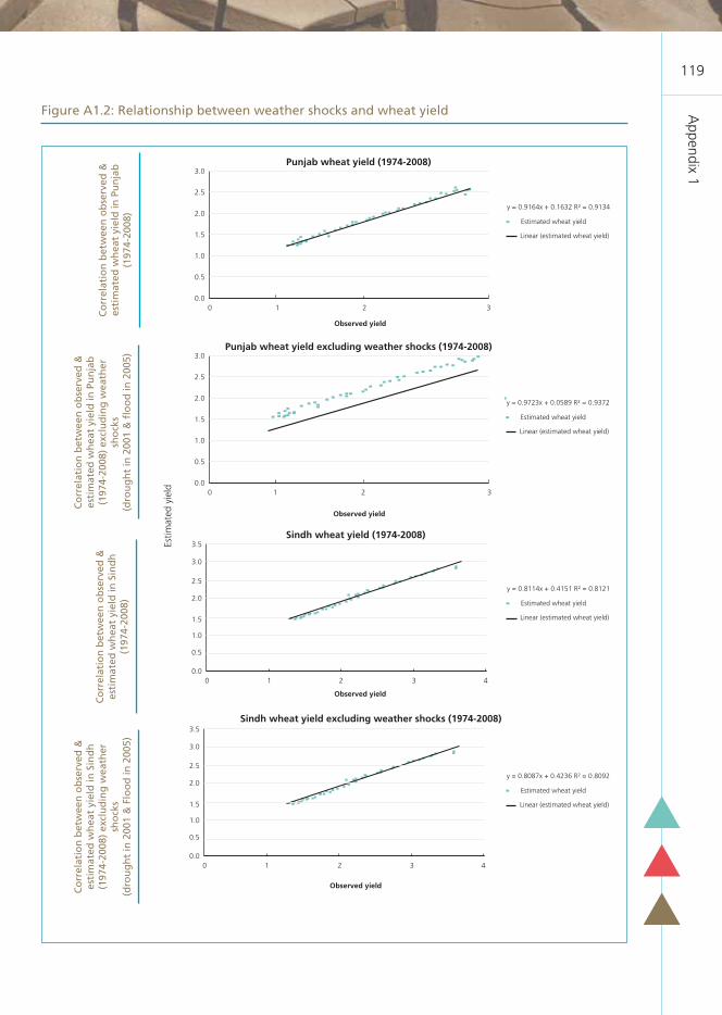
Appendix 1
119
Figure A1.2: Relationship between weather shocks and wheat yield
Co
rrel
atio
n b
etw
een
ob
serv
ed &
es
tim
ated
wh
eat
yiel
d in
Pu
nja
b
(197
4-20
08)
excl
ud
ing
wea
ther
sh
ock
s
(dro
ug
ht
in 2
001
& fl
oo
d in
200
5)
Co
rrel
atio
n b
etw
een
ob
serv
ed &
es
tim
ated
wh
eat
yiel
d in
Sin
dh
(1
974-
2008
)
Co
rrel
atio
n b
etw
een
ob
serv
ed &
es
tim
ated
wh
eat
yiel
d in
Sin
dh
(1
974-
2008
) ex
clu
din
g w
eath
er
sho
cks
(d
rou
gh
t in
200
1 &
Flo
od
in 2
005)
Co
rrel
atio
n b
etw
een
ob
serv
ed &
es
tim
ated
wh
eat
yiel
d in
Pu
nja
b
(197
4-20
08)
0.010 2 3
0.5
1.0
1.5
2.0
2.5
3.0
Observed yield
Punjab wheat yield (1974-2008)
0.0
0.5
1.0
1.5
2.0
2.5
3.0
Estim
ated
yie
ld
Punjab wheat yield excluding weather shocks (1974-2008)
10 2 3
0.010 2 3
0.5
1.0
1.5
2.0
2.5
3.0
3.5
4
Sindh wheat yield (1974-2008)
10 2 3 4
Sindh wheat yield excluding weather shocks (1974-2008)
0.0
0.5
1.0
1.5
2.0
2.5
3.0
3.5
Observed yield
Observed yield
Observed yield
Estimated wheat yield
y = 0.9164x + 0.1632 R² = 0.9134
Linear (estimated wheat yield)
Estimated wheat yield
y = 0.8114x + 0.4151 R² = 0.8121
Linear (estimated wheat yield)
Estimated wheat yield
y = 0.8087x + 0.4236 R² = 0.8092
Linear (estimated wheat yield)
Estimated wheat yield
y = 0.9723x + 0.0589 R² = 0.9372
Linear (estimated wheat yield)

App
endi
x 1
120
Figure A1.2: Relationship between weather shocks and wheat yield - Cont.d
Co
rrel
atio
n b
etw
een
Ob
serv
ed
& E
stim
ated
Wh
eat
Yie
ld in
B
alu
chis
tan
(19
74-2
008)
exc
lud
ing
W
eath
er s
ho
cks
(Dro
ug
ht
in 2
001
&
Flo
od
in 2
005)
Co
rrel
atio
n b
etw
een
Ob
serv
ed &
Es
tim
ated
Wh
eat
Yie
ld in
KPK
(19
74-
2008
)
Co
rrel
atio
n b
etw
een
Ob
serv
ed &
Es
tim
ated
Wh
eat
Yie
ld in
KPK
(19
74-
2008
) ex
clu
din
g W
eath
er s
ho
cks
(Dro
ug
ht
in 2
001
& F
loo
d in
200
5)
Co
rrel
atio
n b
etw
een
Ob
serv
ed &
Es
tim
ated
Wh
eat
Yie
ld in
Pu
nja
b
(197
4-20
08)
Baluchistan wheat yield (1974-2008)
0.0
0.5
1.0
1.5
2.0
2.5
Observed yield
Estim
ated
yie
ld
10 2 3
0.0
0.5
1.0
1.5
2.0
2.5
Observed yield
Estim
ated
yie
ld
Baluchistan wheat yield excluding weather shocks (1974-2008)
10 2 3
Year
-0.5
0.0
0.5
1.0
1.5
2.0
2007
2004
2001
1998
1995
1992
1989
1986
1983
1980
1977
1974
Whe
at y
ield
Wheat yield in KPK (trend & detrended value)
Year
-400-200
0200400600800
1000120014001600
Detrended value
Linear (N_wheat_prod)
N_wheat_prod
2007
2004
2001
1998
1995
1992
1989
1986
1983
1980
1977
1974
Whe
at p
rodu
ctio
n
Wheat production in KPK (trend & detrended value)
Estimated wheat yield
y = 0.5932x + 0.7288 R² = 0.6368
Linear (estimated wheat yield)
Estimated wheat yield
y = 0.5823x + 0.7396 R² = 0.6573
Linear (estimated wheat yield)
Detrended value
Linear (N_wheat_prod)
N_wheat_prod

Appendix 2:
Appendix 2: Simulated results with low DECR (Chapter 6)

App
endi
x 2
122
Table A2.1 Simulated impact of flood and price increases on undernourishment (caloric intake:
% of population <1 730 kcal/per day)
Category POST-SHOCK (2010)
Baseline (2005/2006)
% population <1 730 kcal/day
Scenario 1% population <1 730 kcal/
day
Scenario 2% population <1 730 kcal/
day
% Points Change due to market
shock
% Points Change due
to flood shock
% Points Change due to combined
shock
Rural 23.3 32.7 38.8 9.4 6.2 15.5
Urban 28.9 35.2 35.7 6.2 0.5 6.7
Total 25.5 33.7 37.6 8.1 3. 12.0
MAIN PROVINCES
Punjab 21.7 29.2 31.3 7.5 2.1 9.6
Sindh 33.4 43.3 52.7 9.9 9.4 19.3
KPK 15.1 17.2 18.4 2.1 1.2 3.3
Baluchistan 37.5 52.9 56.2 15.4 3.4 18.8
RURAL LIVELIHOOD GROUPING
Employer * 22.3 33.0 37.5 10.7 4.5 15.2
Paid employee 31.0 44.3 51.1 13.3 6.8 20.1
Unpaid family worker 14.9 24.2 25.4 9.3 1.1 10.4
Owner cultivator 13.3 18.5 25.2 5.2 6.7 11.8
Sharecropper 20.2 26.7 44.2 6.5 17.5 24.0
Contract cultivator 16.5 20.3 24.6 3.9 4.2 8.1
Livestock only 22.2 27.9 33.0 5.8 5.1 10.8
URBAN LIVELIHOOD GROUPING
Agriculture 23.7 30.5 32.3 6.8 1.8 8.6
Traders 30.4 36.3 37.2 5.9 0.9 6.8
Social & personal service
28.1 34.6 35.0 6.4 0.4 6.8
Service sector ** 28.6 35.4 35.8 6.8 0.4 7.2
Industrial sector 28.7 36.0 38.0 7.3 2.0 9.2
INCOME GROUPING-RURAL
Low 29.6 42.2 50.4 12.6 8.2 20.8
Middle 8.2 8.2 8.9 0.0 0.7 0.7
High 2.8 3.6 4.4 0.8 0.7 1.6
INCOME GROUPING-URBAN
Low 51.6 66.1 67.3 14.4 1.2 15.7
Middle 23.2 23.2 22.9 0.0 -0.3 -0.3
High 8.1 9.6 9.8 1.5 0.2 1.7
* Employers is a livelihood group composed of mainly large employers (≥ 10 employees), small employers (<10 employees) and self employed non-agricultural businesses.
** Service sector is an urban livelihood group composed of transport, storage, real estate, & insurance sectors.

Appendix 2
123
Figure A2.1 Percentage of people consuming less than the DECR due to simulated market and
flood shocks by district (% of population below 1 730 kcal/day)
Table A2.2: Simulated shock impacts on the number of undernourished people
(caloric Intake: 000 adults <1 730 kcal/per day)
Category POST-SHOCK (2010)
Baseline (2005/2006)(A)
Scenario 1 Scenario 2(B)
Total (A+B)
Rural 25.971 10.104 16.565 42.536
Urban 18.217 3.933 4.245 22.463
Nationwide 44.188 14.037 20.811 64.999
Scenario 1: market shocks (price increases). Scenario 2: combined floods and price increase.

App
endi
x 2
124
Table A2.3 Depth of hunger among undernourished population (number of kilocalories below
the minimum daily energy requirement of 1 730 kcal/person/day)
Category POST-SHOCK (2010)
Baseline (2005/2006)No. of kcal below
1 730 kcal/day
Scenario 1No. of kcal below
1 730 kcal/day
Scenario 2No. of kcal below
1 730 kcal/day
Rural 296 347 393
Urban 307 363 379
Total 301 353 388
MAIN PROVINCES
Punjab 278 333 354
Sindh 348 385 443
KPK 239 246 255
Baluchistan 303 388 413
RURAL LIVELIHOOD GROUPING
Employer 276 326 361
Paid employee 310 378 407
Unpaid family worker 208 252 359
Owner cultivator 258 269 351
Sharecropper 339 329 460
Contract cultivator 273 257 292
Livestock only 231 311 337
URBAN LIVELIHOOD GROUPING
Agriculture 318 348 412
Traders 323 376 389
Social & personal service 309 359 375
Service sector 277 348 368
Industrial sector 284 345 352
INCOME GROUPING-RURAL
Low 302 353 402
Middle 201 208 208
High 262 250 266
INCOME GROUPING-URBAN
Low 336 401 423
Middle 232 242 241
High 246 265 264
Scenario 1: market shocks (price increases). Scenario 2: combined floods and price increase.

Appendix 2
125
Figure A2.2 Per capita severity of undernourishment due to simulated market and flood shocks
by district (required kilocalories/day to reach minimum daily energy requirement of
1 730 kcal/person/day)
Table A2.4 Quantifying shock impacts in terms of food needed (tonnes of wheat per year) to
meet undernourished requirements
Category POST-SHOCK (2010)
Baseline (2005/2006)(A)
Scenario 1 Scenario 2(B)
Total (A+B)
Rural 827 794 517 903 964 718 1 792 512
Urban 600 484 261 995 313 265 913 749
Nationwide 1 428 278 779 898 1 277 983 2 706 261
Scenario 1: market shocks (price increases). Scenario 2: combined floods and price increase.
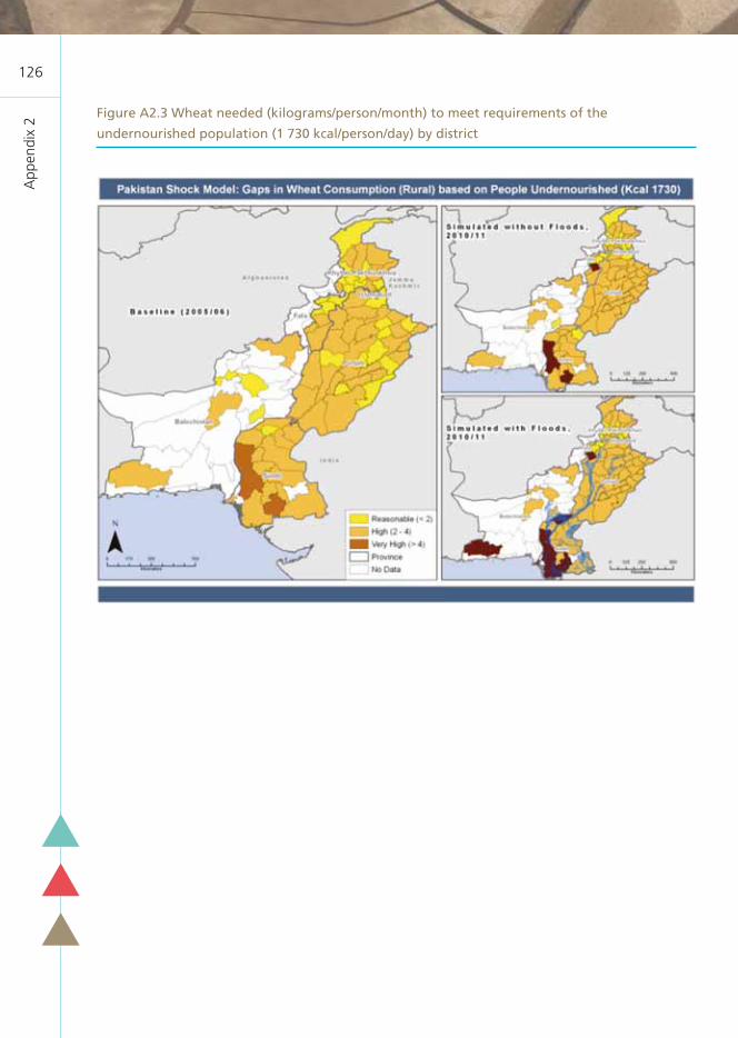
App
endi
x 2
126
Figure A2.3 Wheat needed (kilograms/person/month) to meet requirements of the
undernourished population (1 730 kcal/person/day) by district

Appendix 3: Simulated results with DECR of 2 100 kcal per day (Chapter 6)

App
endi
x 3
128
Table A3.1: Simulated impact of flood and price increases on undernourishment
(caloric intake: % of adults <2 100 kcal/per day)
Category POST-SHOCK (2010)
Baseline (2005/2006)
% population <2 100 kcal/
day
Scenario 1% population <2 100 kcal/
day
Scenario 2% population <2 100 kcal/
day
% Points change due to market
shock
% Points change due
to flood shock
% Points change due to combined
shock
Rural 45.6 54.0 58.7 8.3 4.7 13.0
Urban 51.0 55.2 55.3 4.2 0.1 4.3
Total 47.8 54.5 57.3 6.7 2.9 9.5
MAIN PROVINCES
Punjab 41.8 48.2 50.2 6.4 2.0 8.4
Sindh 57.2 65.7 71.3 8.4 5.6 14.1
KPK 37.7 39.7 40.9 2.0 1.2 3.2
Baluchistan 62.2 73.3 76.3 11.1 2.9 14.0
RURAL LIVELIHOOD GROUPING
Employer 45.9 54.8 58.4 8.9 3.6 12.5
Paid employee 55.3 66.0 70.5 10.7 4.5 15.1
Unpaid family worker 33.5 37.1 43.1 3.6 5.9 9.5
Owner cultivator 31.7 37.4 43.6 5.7 6.2 11.9
Sharecropper 48.1 55.3 67.3 7.2 12.0 19.2
Contract cultivator 34.8 40.4 45.6 5.6 5.2 10.8
Livestock only 40.3 50.0 51.7 9.7 1.7 11.4
URBAN LIVELIHOOD GROUPING
Agriculture 41.1 45.2 47.7 4.0 2.5 6.6
Traders 55.5 59.4 60.1 3.9 0.7 4.6
Social & personal service
49.3 53.3 53.8 4.1 0.4 4.5
Services ector 50.5 56.4 57.2 5.9 0.8 6.7
Industrial sector 53.6 58.6 60.6 5.0 2.1 7.0
INCOME GROUPING-RURAL
Low 55.4 66.3 72.3 11.0 6.0 16.9
Middle 24.7 24.3 24.9 -0.4 0.6 0.2
High 10.9 13.8 16.0 3.0 2.1 5.1
INCOME GROUPING-URBAN
Low 78.3 85.8 86.1 7.4 0.4 7.8
Middle 49.8 50.2 49.6 0.3 -0.5 -0.2
High 22.4 25.6 25.8 3.2 0.3 3.5

Appendix 3
129
Table A3.2: Simulated shock impacts on the number of undernourished people
(caloric intake: 000 adults <2 100 kcal/per day)
Category POST-SHOCK (2010)
Baseline (2005/2006)(A)
Scenario 1 Scenario 2(B)
Total (A+B)
Rural 50 535 8 899 13 802 64 337
Urban 32 140 2 639 2 714 34 855
Nationwide 82 675 11 538 16 516 99 192
Scenario 1: market shocks (price increases). Scenario 2: combined floods and price increase.

App
endi
x 3
130
Table A3.3: Depth of hunger among undernourished population (number of kilocalories below
the minimum daily energy requirement of 2 100 kcal/person/day)
Category POST-SHOCK (2010)
Baseline (2005/2006)No. of kcal below 2
100 kcal/day
Scenario 1No. of kcal below
2 100 kcal/day
Scenario 2No. of kcal below
2 100 kcal/day
Rural 429 509 570
Urban 465 537 551
Total 445 520 562
MAIN PROVINCES
Punjab 425 502 524
Sindh 494 563 652
KPK 351 371 381
Baluchistan 483 603 629
RURAL LIVELIHOOD GROUPING
Employer 409 490 539
Paid employee 463 566 616
Unpaid family worker 413 463 485
Owner cultivator 366 407 495
Sharecropper 407 441 618
Contract cultivator 388 402 434
Livestock only 409 466 524
URBAN LIVELIHOOD GROUPING
Agriculture 478 539 581
Traders 463 533 547
Social & personal service 468 540 553
Service sector 452 518 533
Industrial sector 438 518 521
INCOME GROUPING-RURAL
Low 445 531 597
Middle 309 313 324
High 282 278 282
INCOME GROUPING-URBAN
Low 532 641 664
Middle 382 384 382
High 333 356 355
Scenario 1: market shocks (price increases). Scenario 2: combined floods and price increase.

Appendix 3
131
Table A3.4: Quantifying shock impacts in terms of food needed (tonnes of wheat per year) to
meet undernourished requirements of 2 100 kcal/day
Category POST-SHOCK (2010)
Baseline (2005/2006)(A)
Scenario 1 Scenario 2(B)
Total (A+B)
Rural 2 340 301 916 993 1 587 307 3 927 608
Urban 1 605 408 400 223 456 687 2 062 094
Nationwide 3 945 709 1 317 216 2 043 994 5 989 703
Scenario 1: market shocks (price increases). Scenario 2: combined floods and price increase.


Appendix 4: Introduction - FAO/WFP SISMod

App
endi
x 4
134
2013
A tool to measure the impact of shocks on food security in vulnerable countries
Project rationale• The FAO/WFP Shock Impact Simulation Model (SISMod) has been developed to address
the notable rise in the number of people facing various types of shocks (market, economic, political and climatic), which leads to challenges in addressing food insecurity in developing countries. Previously, it had proved difficult to provide quantitative estimates on the impact that various shock factors have on the livelihoods and food security of different population groups at a nationally representative level.
• Shocks arise from rapid changes in economic, political, market or climatic conditions, and affect different population groups differently. These shocks can have lasting impacts on livelihoods and food security, impeding development and progress. Interventions are often criticised for being “too little, too late”, but often actors do not have the necessary tools to make quantitative assessments that can help them identify who is most affected, to what extent and where.
• The initial phase of the current project focused on shock-prone food-deficit countries representing different levels of exposure to shocks: Bangladesh, Nepal, Pakistan, Tajikistan, Niger, Tanzania and Uganda.
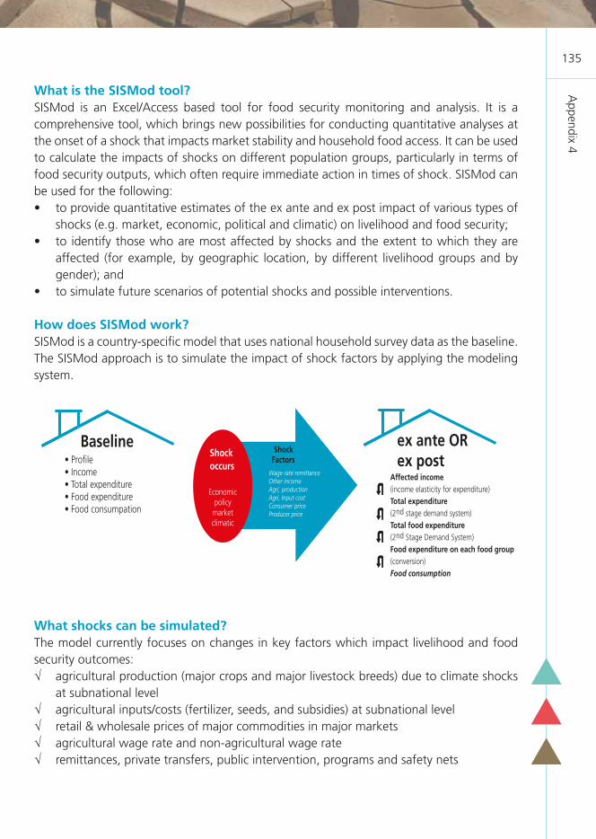
Appendix 4
135
What is the SISMod tool?SISMod is an Excel/Access based tool for food security monitoring and analysis. It is a comprehensive tool, which brings new possibilities for conducting quantitative analyses at the onset of a shock that impacts market stability and household food access. It can be used to calculate the impacts of shocks on different population groups, particularly in terms of food security outputs, which often require immediate action in times of shock. SISMod can be used for the following:• to provide quantitative estimates of the ex ante and ex post impact of various types of
shocks (e.g. market, economic, political and climatic) on livelihood and food security; • to identify those who are most affected by shocks and the extent to which they are
affected (for example, by geographic location, by different livelihood groups and by gender); and
• to simulate future scenarios of potential shocks and possible interventions.
How does SISMod work?SISMod is a country-specific model that uses national household survey data as the baseline. The SISMod approach is to simulate the impact of shock factors by applying the modeling system.
What shocks can be simulated?The model currently focuses on changes in key factors which impact livelihood and food security outcomes: agricultural production (major crops and major livestock breeds) due to climate shocks
at subnational level agricultural inputs/costs (fertilizer, seeds, and subsidies) at subnational level retail & wholesale prices of major commodities in major markets agricultural wage rate and non-agricultural wage rate remittances, private transfers, public intervention, programs and safety nets
Baseline• Profile• Income• Total expenditure• Food expenditure• Food consumpation
ex ante ORex post
Affected income(income elasticity for expenditure)Total expenditure(2nd stage demand system)Total food expenditure(2nd Stage Demand System)Food expenditure on each food group(conversion)Food consumption
Wage rate remittanceOther incomeAgri, productionAgri, Input costConsumer priceProducer price
Shockoccurs
Economicpolicymarketclimatic
ShockFactors

App
endi
x 4
136
macro-economic factors and trade policies (including consumer price index, exchange rate, tariff, population)
KEY output indicators for interventionsThe model generates estimates of the impacts on key livelihood variables as listed below: • proportion of people consuming less than a specified level of dietary energy consumption
(DEC) (i.e. below a specified threshold); • number of people who need food assistance after shocks;• depth of hunger (kcal/person/day), i.e. deficit in absolute terms between the average
DEC of the needy population and the threshold level;• gap of food needs (kg of cereal/person/year), i.e. cereal needed to meet the needs of
the undernourished population;• total food assistance needed to meet the needs (ton/year); • agricultural assistance needs after shocks;• indicators for gender/smallholder/MDG studies;• changes in household income and expenditure;• changes in agricultural production and food availability; and• other indicators as requested.
Outputs display optionsIn the SISMod tool, the outputs are listed on the “OUTPUT tab” and presented in table and chart format for quick reference and use:
Output indicators by groupsFor better targeting, the shock impacts at household level are aggregated by various groupings, and the outputs can be viewed by different population groups, including:

Appendix 4
137
Grouping for geographical analysis for food distribution• nationwide total • by living area (Urban/Rural)• by province (e.g. Pakistan: Punjab/Sindh/Khyber Pakhtunkhwa/Balochistan)• by district (e.g. Pakistan: covering 82 out of 102 districts)• by district & living area
Grouping by gender index for gender analysis• by gender of household head & living area• by index on the ratio of females within household & living area • by index on the ratio of female adults (age 15-64) within household & living area• by gender and marital status of household head
Grouping by production/land ownership size for smallholder family farming analysis • by index on land size (operated)• by index on per capita production quantity• by index on per capita value of production sold
Grouping by income/income source for poverty analysis• by income group & geographic area• by industry type of household head & geographic area• by employment status of household head & geographic area
Other groupings based on the objectives of the intervention program and policy analysis.
Applying the outputs The model can be used for comprehensive situation analysis, simulation and monitoring of the impact of shocks on household livelihoods and food consumption. It can also generate values for estimated populations with food needs, which can be used in WFP operations and other interventions.
By regularly updating the time series data, the model can be used to monitor situations of changing market conditions. Such regular updates would enable the SISMod to be applied in crisis situations.
For policy purposes, the model can be used to deduce the effect of shocks in past situations and draw lessons for future shocks, in order to better understand how to target interventions to protect those at the greatest risk of loss of income and food consumption. The model is country specific; users will observe that the impact of shocks is largely context specific. Similar shocks in different parts of the country can lead to similar or different outcomes, depending on the type of shock, its magnitude and the profile of the household. The model can be run and compared with the results from other countries to better understand the need to tailor interventions and policy in food security to country needs.

App
endi
x 4
138
The quantitative estimates supplied by SISMod can be used to support other impact assessments, such as the Household Economic Analysis or WFP and FAO emergency assessments.
Potential usersSISMod allows timely assessment of emerging issues by generating up-to-date subnational food security data, and simulates the outcome of different intervention/policy scenarios. This will be valuable to a wide range of potential users including WFP, FAO, and national/international aid bodies who carry out Food Assistance Interventions and Economic/Policy Analysis on:• crop and food security assessments (e.g. CFSAM)• rapid or emergency food security assessments after disasters and market shocks (e.g. EFSA)• rapid market situation assessments (e.g. EMMA, MIFIRA)• joint UN MDG assessments• programme formulation activities (e.g. emergency operations, recovery and rehabilitation)• disaster risk planning • gender impact analysis• smallholder and trade policy analysis
Structure of SISModThe tool combines data sets from FAO, WFP, World Bank and national sources on key household/livelihood, economic, market and production data to model the effect of various key shock factors.
The conceptual model of SISMOD is shown in the following diagram:
MODEL STRUCTURE FOR SIMULATING SHOCKS
Shock factors Food securityIncome
Wage ratesremittances
CPI
Gross income
Other income
Income from crop
& livestock
Foodexpenditure
Foodconsumption
Foodneeds
Elasticityestimations
Totalexpenditure
Input costs
Consumer retail prices
Producer wholesale
prices
Crop production
Population
Time frame
Economic & policy
Market
Climate
Shock Occurs(economic or
climatic)
Impact on livlihoods
Step 1: Input key parameters
Simulation profile
Step 2: Adjust shock factors Step 3: Run model & analysis ouputs

Appendix 4
139
What is the methodology used?SISMod adopts the Agricultural Household Model (AHM) approach developed by Singh et al. (1986). The AHM incorporates both the production and consumption sides. It integrates the price effects on different markets and takes into account the interactions between them. The fundamental difference between an AHM and pure consumer model is that the household budget is generally assumed to be fixed in a pure consumer model, while in AHM it is endogenous, and depends on production decisions that contribute to income through farm profits in AHM. The traditional price effect is composed of the farm profits effect (as a producer), which adds a positive influence to the negative Slutsky effects on food demand (as a consumer). Similarly, other income factors such as remittance, wage rate and safety net/transfers have been modelled through household income equations.
The foundation of the SISMod analysis is built on a series of modules that take into account household income and expenditure, and estimates demand/supply/price transmission elasticities based on household survey data, national sources on food prices and other assessments. SISMOD works by linking together components such as market monitoring, crop production monitoring, the income generation module, a two-stage household budget allocation module, and changes in shock factors.
These modules track the changes in shocks factors based on either a) past patterns linked to the VAM or GIEWS monitoring systems, or b) forecasts based on a partial equilibrium model or short term price analysis. The household income module includes the following components: crop & livestock income, wage income, remittance income, and other income. To pass on the shock effects to income and then to total household expenditure, the household average propensity to consume (APC) is estimated by using household survey data.
The demand side module consists of a two-stage food demand system. The first stage allocates total household expenditure to broad groups of goods such as food, clothing, fuel, housing, durable goods, education, medical items, and other items. A nonlinear seemingly unrelated regression was used to estimate a linear expenditure system (LES) of equations for the first-stage budget allocation. In the second stage, the food demand equation for each food item is defined as a function of the real price of the commodity, real consumer expenditures per capita, and real prices of other foods.
The real price of the commodity is expected to be negatively related to food demand. The signs of the other two variables are ambiguous because expenditure elasticities can be positive or negative, and other foods can be substitutes or complements. The model bases these calculations on the national and subnational context where possible. Given the income and price elasticities, the percentage change in each food item consumed will be determined by the percentage change in price (own and cross price) and percentage change in income.
Deriving per capita dietary energy consumption: Food consumption in quantities is converted into dietary energy consumption by using energy conversion factors for energy-

App
endi
x 4
140
yielding macronutrients (protein, fat and carbohydrates). Food consumption is usually measured at the household level, so we define the household level quantity of food and the total dietary energy intake, measured in kilocalories per household. The changes in dietary energy consumption are given by the changes in food consumption.
Deriving Food Needs: The food energy gap refers to the condition of people whose dietary energy consumption is continuously below minimum dietary energy consumption needs for maintaining a healthy life and carrying out light physical activity. The minimum dietary energy consumption need for a specified age and sex group in the household is estimated, based on household members’ age and gender.
SISMod also allows users to have additional options to establish different thresholds to run in the same analysis for different policy intervention objectives. The estimated additional food assistance needs as a result of shocks is measured as the cereal (e.g. maize) equivalent weight (kg).
(For a more detailed explanation of the methodology, please refer to Section Two of this book.)
How do you run the model?The complete SISMod tool consists of two files:
a) Excel - SISMod_PAK_v1.xlsm and b) Access - SISMod_PAK_v1.accdb
These files have to be saved in a specific folder: C:\FAO_WFP_ShockModel\Pakistan (i.e. a main folder FAO_WFP_ShockModel, with a subfolder Pakistan).
Microsoft Excel (2007 or above) and Microsoft Access (2007 or above) are required to run the model. Depending on computer processing speed, it may be necessary to close all other open files and programs, to ensure that the SISMod tool processes properly (because of its large database).
Users have to make an effort to familiarize themselves with the SISMod methodology in order to ensure that the data input is accurate, model outputs are accurately interpreted. The step-by-step instructions given in the user manual should be followed throughout the modelling excise. Three main steps are required to run the model:
1. Input key parameters: a) Users select the time frame (shock year) of the shock, define the boundaries of
minimum dietary intake according to analysis or intervention need. Users also have to update or forecast the market and economic data series at subnational level or national level by using the modules and past data in the model.

Appendix 4
141
b) The SISMod tool projects the population size for the shock year and computes shock factors based the data series inputted.
2. Adjust shock factors (optional): If users need to further adjust the shock factors to create scenarios, they have to input the percentage change from the baseline for each shock factor which is being modelled. Single or multiple shock shocks can be changed, depending on the scenario.
3. Run model and analyse outputs: a) Users trigger the running of the model by one-click.b) The SISMod tool simulates key livelihood and food security indicators reflecting
shock impacts: income/expenditure, food expenditure, food consumption and food assistance needs, with options to account for livelihood, gender and geographical differences.
For more information please contact:
Cheng Fang, FAO (EST) [email protected] Sanogo, WFP (VAM) [email protected]


