Food Demand Elasticities in Ethiopia: Estimates Using Household Income Consumption Expenditure (HICE)

Survey Data

Kibrom Tafere, Alemayehu Seyoum Taffesse, and Seneshaw Tamiru

with Nigussie Tefera and Zelekawork Paulos

Development Strategy and Governance Division, International Food Policy Research Institute – Ethiopia Strategy Support Program 2, Ethiopia

IFPRI-Addis Ababa P.O. Box 5689 Addis Ababa, Ethiopia Tel: +251-11-646-2921 Fax: +251-11-646-2318 E-mail: ifpri-addis@cgiar.org

IFPRI HEADQUARTERS International Food Policy Research Institute 2033 K Street, NW • Washington, DC 20006-1002 USA Tel: +1-202-862-5600 Skype: IFPRIhomeoffice Fax: +1-202-467-4439 E-mail: ifpri@cgiar.org www.ifpri.org

ESSP2 Discussion Paper 011

Ethiopia Strategy Support Program 2 (ESSP2)

Discussion Paper No. ESSP2 011

April 2010

THE ETHIOPIA STRATEGY SUPPORT PROGRAM 2 (ESSP2)

DISCUSSION PAPERS

ABOUT ESSP 2

The Ethiopia Strategy Support Program 2 is an initiative to strengthen evidence-based policymaking in Ethiopia in the areas of rural and agricultural development. Facilitated by the International Food Policy Research Institute (IFPRI), ESSP 2 works closely with the government of Ethiopia, the Ethiopian Development Research Institute (EDRI), and other development partners to provide information relevant for the design and implementation of Ethiopia‟s agricultural and rural development strategies. For more information, see http://www.ifpri.org/book-757/ourwork/program/ethiopia-strategy-support-program or http://www.edri.org.et/.

.

ABOUT THESE DISCUSSION PAPERS

The Ethiopia Strategy Support Program 2 (ESSP2) Discussion Papers contain preliminary material and research results from IFPRI and/or its partners in Ethiopia. The papers are not subject to a formal peer review. They are circulated in order to stimulate discussion and critical comment. The opinions are those of the authors and do not necessarily reflect those of their home institutions or supporting organizations.

About the Author(s)

Kibrom Tafere International Food Policy Research Institute, Ethiopia Strategy Support Program

Alemayehu Seyoum Taffesse International Food Policy Research Institute, Ethiopia Strategy Support Program Seneshaw Tamiru International Food Policy Research Institute, Ethiopia Strategy Support Program Nigussie Tefera Zelekawork Paulos International Food Policy Research Institute, Ethiopia Strategy Support Program International Food Policy Research Institute, Ethiopia Strategy Support Program

Food Demand Elasticities in Ethiopia: Estimates Using Household Income Consumption Expenditure (HICE) Survey

Data

Kibrom Tafere, Alemayehu Seyoum Taffesse, and Seneshaw Tamiru with Nigussie Tefera and Zelekawork Paulos

Development Strategy and Governance Division, International Food Policy Research Institute –

Ethiopia Strategy Support Program 2, Ethiopia

Copyright © 2010 International Food Policy Research Institute. All rights reserved. Sections of this material may be reproduced for personal and not- for-profit use without the express written permission of but with acknowledgment to IFPRI. To reproduce the material contained herein for profit or commercial use requires express written permission. To obtain permission, contact the Communications Division at ifpri-copyright@cgiar.org.

Table of Content

ACKNOWLEDGMENTS ............................................................................................................. 1

1. INTRODUCTION ................................................................................................................ 2

2. METHODOLOGY ................................................................................................................ 3

3. DATA .................................................................................................................................. 6

4. ESTIMATION STRATEGY .................................................................................................. 7

5. RESULTS ..........................................................................................................................15

6. CONCLUSIONS .................................................................................................................20

REFERENCES .........................................................................................................................21

APPENDICES ...........................................................................................................................31

APPENDIX II: DERIVATION OF ELASTICITY OF DEMAND FOR QU-AIDM ...........................45

List of Tables

Table 1a: Compensated Price Elasticities (Country-level) .........................................................16

Table 1b: Compensated Price Elasticities of Cereals (National) ................................................17

Table 2: Expenditure Shares and Expenditure Elasticities ........................................................18

Table 3: Price Elasticities of Cereals (Urban/Rural) ...................................................................19

Table 4: Compensated Price Elasticity of Demand (QU-AIDM) – Country-level ........................24

Table 5a: Compensated Price Elasticity of Demand by Location (QU-AIDM) - Rural ................26

Table 5b: Compensated Price Elasticity of Demand by Location (QU-AIDM) - Urban ...............27

Table 6: Summary of Own Price Elasticities (QU-AIDM) ...........................................................28

Table 7: Comparison of Own Price Elasticity of Demand Estimates ..........................................29

Table 8: Elasticity Estimates from Alternative Demand Models or Estimation Procedures ........30

Table 9.1: IFGNLS Estimates of the QU-AIDM Parameters – Country-level ..............................31

Table 9.1 cont‟d ........................................................................................................................33

Table 9.2: IFGNLS Estimates of the QU-AIDM Parameters – Rural ..........................................35

Table 9.2 cont‟d ........................................................................................................................37

Table 9.3: IFGNLS Estimates of the QU-AIDM Parameters – Urban .........................................39

Table 9.3 cont‟d ........................................................................................................................41

Table 10 – Households with zero expenditure, by commodity group .........................................43

Table 11: Commodity Groups ...................................................................................................44

Table 12: Estimated Quality (or expenditure) Elasticity of Unit Values ......................................47

1

ACKNOWLEDGMENTS

The authors would like to thank Paul Dorosh for his sustained interest and regular dialogue

throughout the evolution of the paper. They acknowledge the assistance of Miguel Robles and

Brian Poi, as well as the comments ofESSPII conference participants. The authors also thank

the Ethiopian Central Statistical Agency (CSA) for providing the data used. All the usual caveats

apply.

2

1. INTRODUCTION

How households adjust their consumption in response to changes in prices and income is

crucial determinant of the effects of various shocks to market prices and commodity supplies.

These adjustments in demand are particularly significant in Ethiopia, where many households

consume inadequate quantities of calories, protein and other nutrients. Household consumption

behaviour in the country is also rather complex. Regional consumption patterns differ

considerably with no single staple dominating. Instead, four different cereals (teff, wheat,

maize and sorghum) are major staples in parts of the country and even within most regions, two

or more food staples account for relatively large shares of total calories and food expenditures1.

Quantifying household responses to price and income changes requires careful econometric

analysis of household consumption patterns. This paper utilizes household level data on

consumption, prices, expenditures, and household characteristics (including location, size, and

education of household head) to estimate demand parameters for various commodity groups.

The Quadratic Almost Ideal Demand Model (QU-AIDM) was used for that purpose. The QU-

AIDM has solid theoretical foundations and sufficient flexibility to capture substitution effects that

are especially important in the Ethiopian context of multiple staple foods.

The recent unprecedented rise in food prices in Ethiopia renewed interest in the empirical

analysis of consumer demand.2 Coupled with the paucity of current and Ethiopia-specific

demand elasticities estimates, this interest makes the present study timely. Indeed, robust

income and price elasticities of demand not only deepen understanding of economic behaviour

in the country, but can also enhance policy analysis by serving as important ingredients to such

efforts as welfare evaluations and CGE analyses.

1 Enset („false banana‟) is also a major staple in the highland areas of Southern Nations, Nationalities and Peoples region (SNNP).

2 See for instance Ulimwengu, Workneh, and Paulos (February 2009); TEFERA (AUGUST 2009); and TEFERA, NIGUSSIE, RASHID, AND

TAFFESSE (AUGUST 2009).

3

2. METHODOLOGY

Model

Consumer demand theory characterizes the basic problem of a consumer as that of maximizing

utility subject to a budget constraint.3 Under a set of assumptions, this optimization results

demands which:(i) add-up to total expenditure (value form) or to one (budget-share form), (ii)

are homogeneous of degree zero in prices alone (compensated or Hicksian demands), or jointly

in prices and total expenditure (uncompensated or Marshallian demands), (iii) have negative

compensated own-price responses, and (iv) exhibit symmetric compensated cross-price

responses (Deaton and Muellbauer (1980a)).4 As can be expected, testing the validity of this

characterization occupies a major place in empirical demand analysis. In this regard, it is

common practice to specify functional forms (for utility or expenditure) that are flexible enough

to lead to demands possessing the above properties, such that the relevant restrictions are

statistically imposed and tested. As a prelude to empirical implementation this section describes

the demand models adopted in this study.

One of the most commonly used specifications in applied demand analysis is the Almost Ideal

Demand Model (AIDM) proposed by Deaton and Muellbauer (1980b). Its popularity is in part

due to the fact that it satisfies a number of desirable properties5 and allows linear approximation

at the estimation stage. The model has budget shares as dependent variables and logarithm of

prices and real expenditure/income as regressors.

The original AIDM was subsequently extended to permit non-linear Engel curves. The resulting

model, proposed by Banks, Blundell, and Lewbel (1997), is the Quadratic Almost Ideal Demand

Model(QU-AIDM). Under QU-AIDM, the ith budget share (wi) equation for household h is given

by:6

2

1

ln ln ln (1)( ) ( ) ( )

nh i h

ih i ij j ij

x xw p

a b ap p p

with:

3 As will be seen shortly, the bulk of the data used by this study are at the household level. The household is assumed to behave as

if it were a single consumer. This approach is known as the „unitary approach‟ to household consumption behaviour. An alternative, broadly known as the „collective approach‟, attempts to accommodate the possible preferential and other heterogeneity of household members. The latter is rapidly growing in acceptance as a better perspective. See Browning, Chiappori, and Lechene (2006) for a recent elaboration of the difference between the two approaches. 4 The classic statement of this is Chapter 2 in Deaton and Muellbauer (1980a).

5 AIDM satisfies axioms of choice exactly; it allows exact aggregation over consumers; is simple to estimate; and it can be used to

test the restriction of homogeneity and symmetry through linear restrictions on fixed parameters (see Deaton and Muellbauer (1980b); and Moschini (1995)). 6 Note that with λi=0 the QU-AIDM reduces to the original AIDM.

4

01 1 1

1ln ( ) ln ln ln (2)

2

n n n

k k kj k jk k j

a p p pp

1

( ) (3)k

n

kk

b pp

In equations (1)−(3), pj and x stand for the price of commodity j and total consumption

expenditure, respectively, while ln() indicates logarithmic transformation. The αs, βs, γs, and λs

are parameters to be estimated.

Three main properties of demands derived from utility maximization under a budget constraint

can be stated and tested as restrictions on the parameters of the QU-AIDM equation system

(1).7 These are:

1 1 1

1; 0; 0; 0 (4) n n n

i ij i ii i i i

0 (5)ijj

(6)ij ji

The equalities in (4) are the adding-up restrictions. They express the property that the sum of

the budget shares equals 1 (i.e.1ihw

). The restrictions (5) express the prediction that the

demand functions are homogenous of degree zero in prices and expenditure/income. Slutsky

symmetry is satisfied only if the restrictions in (6) hold.

If the restrictions in equations (4)-(6) are satisfied, it would imply (Deaton and Muellbauer

[1980b, 314]):

1) With no variation in relative prices and ‘real’ expenditure (x/a(P)), the budget shares are

constant.

2) The direct impact of relative prices appears through the coefficients γij , each representing 100

times the effect on the ith budget share of a 1 percent increase in the jth price with (x/a(P)) held

fixed.

3) A change in ‘real’ expenditure work through the terms βi and λi.

7 Note that negativity of own-price responses cannot be imposed in the form of restrictions on the parameters of the model. See

Deaton and Muellbauer (1980b).

5

A number of additional features, to be introduced below to accommodate various data and

estimation issues, will modify the form in which these implications, as well as the restrictions

they are based on, apply.

6

3. DATA

The analysis in this paper is primarily based on data collected by the Central Statistical Agency

(CSA) via its Household Income Consumption Expenditure Survey (HICES) during 2004/05.

Additional information was extracted from the Welfare Monitoring Survey (WMS) of the same

year. 8 The HICES covers all rural and urban areas of Ethiopia except all zones of the Gambella

region, and three predominantly non-sedentary zones from Afar region and six such zones from

Somali region.

For the purpose of HICES 2004/05, CSA divided the country into three broad categories: „rural‟,

„major urban centres‟ and „other urban centres‟ categories. The „rural‟ category consists of all

rural areas in all regions of Ethiopia except those noted earlier. „Major urban centres‟ consists

mainly of regional capitals and four other urban centres with relatively sizable populations, while

„other urban centres‟ includes all urban areas that do not fall under „major urban centres‟

category.9 A total of 21,595 households make up the HICES sample. This nationally

representative sample contains 12,101 urban households and 9,494 rural households selected

from 1554 enumeration areas (EAs) in 444 woredas.

The HICES collect information on quantity of consumption, consumption expenditure, and other

expenditures of households. In contrast, the WMS survey focuses on assets, health, education,

nutrition, access to and utilization and satisfaction of basic facilities/services. Hence, the

expenditure data from HICES (2004/05) are combined with the information on assets and

demographics drawn from WMS (2004).

8 Detailed description of the HICES and the WMS can be respectively found in CSA (May 2007) and CSA (June 2004).

9 According to CSA, an urban area is generally defined as a locality with 2000 inhabitants or more. However, in the HICE (2004/05)

survey urban areas are:

i) All administrative capitals (Regional capitals, Zonal capitals and Wereda capitals); ii) Localities with Urban Dwellers‟ Association (UDAs) not included in (i); and

iii) All localities which are not included either in (i) or (ii) above, having a population of 1000 or more persons, and whose inhabitants are primarily engaged in non- agricultural activities.

7

4. ESTIMATION STRATEGY

This section describes the key elements of the estimation strategy deployed in this paper. The

strategy is adopted to address a number of issues including endogeneity of total expenditure to

budget shares, the use of unit values in place of market prices, and the case of zero

expenditures.

Unit values

The HICES dataset does include a set of prices. Nevertheless, consultation with CSA revealed

that it is not advisable to use these prices in the analysis. It was thus necessary to explore

alternatives. One option was presented by the data on expenditures on and quantities of

commodities collected by the HICE survey. It is as a result possible to calculate the unit value of

each commodity as the ratio of expenditures and quantities for households with data on both.

Data on expenditure, or quantity, or both are not reported for some households. Some of these

households did not purchase the commodity during the survey period, while others did but part

or all of the information on their purchase is not recorded. Consequently, missing unit values are

replaced by the mean unit value of the corresponding EA, Kebele, Woreda, zone, or region,

whichever occurs first. The unit values thus computed are used as „prices‟. More specifically, for

each commodity the household-level unit value takes the place of the corresponding price in

estimating price responses of commodity demands.10

The use of unit values as prices has some problems which have been thoroughly examined in

Deaton (1987; 1988; 1990; 1997) and more recently in Crawford, Laisney, and Preston (2003)

and Kedir (2005). The following paragraphs highlight the major concerns identified so as to put

the paper‟s empirical results in perspective.

Two main complications arise from the use of unit values even when they are assumed to be

direct indicators of corresponding prices (Deaton (1997)). The first relates to quality

differentiation within a commodity subgroup. Take wheat, for instance. It comes in several

varieties and quality grades. These types, varieties, or grades are unlikely to be valued equally

by consumers or have a uniform price. The unit value of wheat thus reflects these quality

differences. Household choice among goods differentiated by quality, in turn, is likely to be

influenced by prices. The price of a commodity therefore affects unit values directly and through

quality choice. Whenever operational, the latter effect prevents unit values from moving one to

one with corresponding prices. Clearly, this complication is likely to be more severe when

commodities are aggregated into groups with two or more constituents. In this regard, assuming

group-separable preferences Deaton (1987; 1988) demonstrates that the unit value of a

10

In this regard TEFERA (AUGUST 2009) and TEFERA, NIGUSSIE, RASHID, AND TAFFESSE (AUGUST 2009) also adopted this solution. The strategy deployed by Ulimwengu, Workneh, and Paulos (February 2009) is not explicitly discussed in the paper.

8

commodity group will have a less than proportionate response to the price of the group if the

aforementioned quality effect is present. The solution he proposes involves correcting quantities

and unit values for quality differences before estimating a quantity-unit value relation.

Measurement error is the second problem. Expenditures and quantities are measured with

errors. Unit values, being ratios of the two, are thus contaminated by those errors. Deaton

(1988) illustrates that these errors are likely to be spuriously negatively correlated with recorded

quantities. Estimating the relationship between quantities and unit values without accounting for

measurement error can hence results in biased estimates of the price responses of demand.

In short, quality differences within commodity groups and errors of measurement in

expenditures and quantities can lead to biased estimates. As a solution (Deaton, 1987)

proposes a complicated errors-in-variables estimator corrected for quality. Implementing this

estimator is not attempted here. Apart from the view that such implementation merits a separate

treatment in its own right, a number of considerations led to this decision.

First, „quality‟ elasticity of unit values were estimated and did not prove to be very large. For

food commodities, these elasticities range from -0.018 for sorghum through to 0.1722 for „sugar

and salt‟ (Table 9). Elasticities of comparable magnitude are also reported in Kedir (2005) for

urban Ethiopia. As expected the quality divergence caused by income/expenditure differences

are much wider in the case on non-food commodities. Second, the quantitative significance of

adjustments for „quality‟ effects and measurement error associated with the use of unit values

does not appear to be large. Kedir (2005) obtains estimates of „price‟ elasticities of quantity

demanded for urban Ethiopia that correct for these problems. He concludes “(s)pices, fruits and

vegetables, and tella have relatively large quality corrections. Teff, cereals, shiro, oil, meat, milk

and butter have modest corrections followed by slight corrections for wheat, pulses, coffee and

sugar.” In other words, from among his 13 commodities only three, and none of them a staple,

have sizable corrections (see Table 3 in Kedir (2005)). Third, the level difference between unit

values and prices may not be considerable. Capéau and Dercon (2005) implemented a

regression-based adjustment procedure to correct unit values. Out of the 15 cite-crop specific

mean unit values, only 4 fell outside the 95% confidence interval of the corrected „price‟

estimates (see Table 4 in Capéau and Dercon (2005)). To conclude, the present paper‟s

estimates of price responses of demands are obtained on the basis of unit values.11

11

Two further points. Even when adjustments are made for quality effects and measurement error, it is still necessary to establish the significance of the results thereby obtained via a comparison with an analogous estimation using observed prices. Furthermore, if measurement error is the main culprit, the bias may not necessarily be eliminated by using directly collected prices, since the latter may also be measured with substantial error. The findings in Deaton (1987, 1988, 1990), though not necessarily applicable in general, suggest that relative to quality differentiation, measurement error is by far the more significant source of bias. Indeed it is not possible to infer a priori that the potential bias associated with unit values is necessarily worse than that related to prices.

9

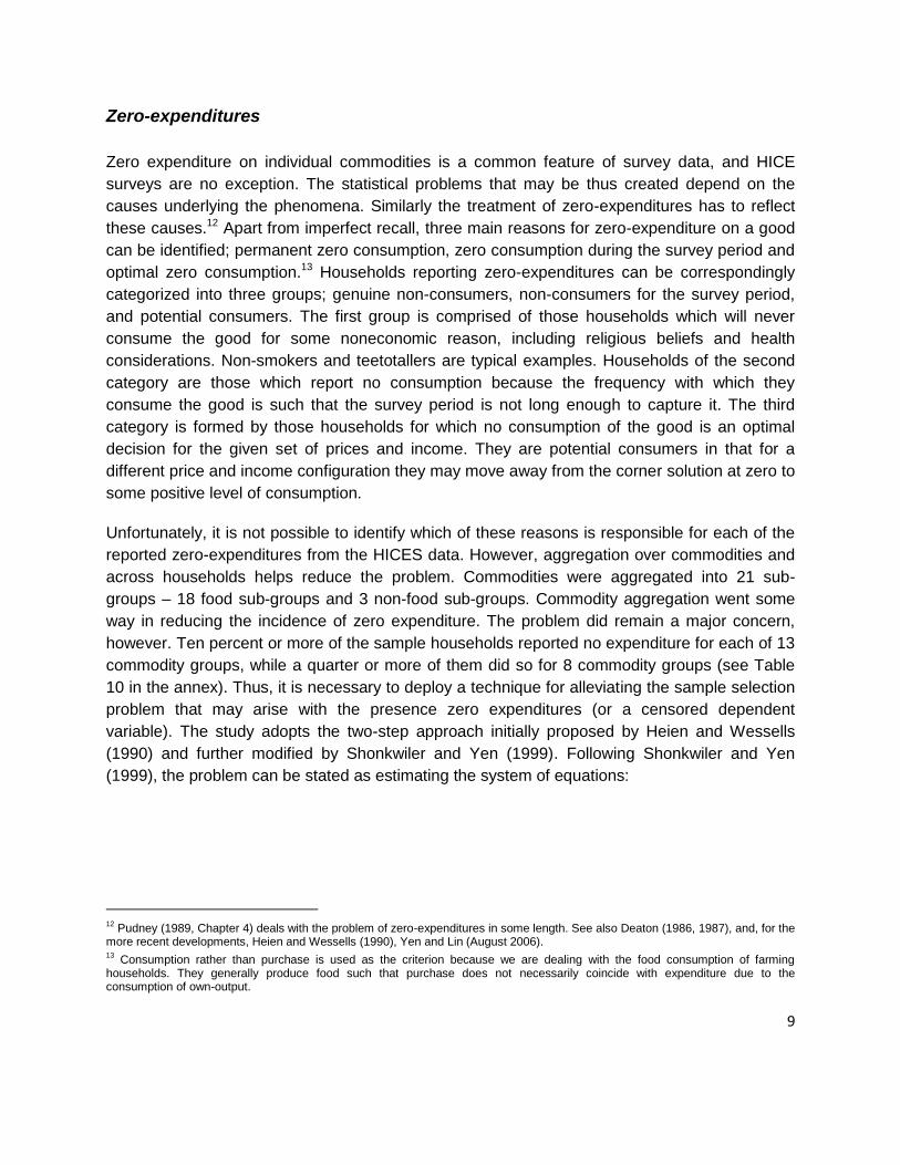
Zero-expenditures

Zero expenditure on individual commodities is a common feature of survey data, and HICE

surveys are no exception. The statistical problems that may be thus created depend on the

causes underlying the phenomena. Similarly the treatment of zero-expenditures has to reflect

these causes.12 Apart from imperfect recall, three main reasons for zero-expenditure on a good

can be identified; permanent zero consumption, zero consumption during the survey period and

optimal zero consumption.13 Households reporting zero-expenditures can be correspondingly

categorized into three groups; genuine non-consumers, non-consumers for the survey period,

and potential consumers. The first group is comprised of those households which will never

consume the good for some noneconomic reason, including religious beliefs and health

considerations. Non-smokers and teetotallers are typical examples. Households of the second

category are those which report no consumption because the frequency with which they

consume the good is such that the survey period is not long enough to capture it. The third

category is formed by those households for which no consumption of the good is an optimal

decision for the given set of prices and income. They are potential consumers in that for a

different price and income configuration they may move away from the corner solution at zero to

some positive level of consumption.

Unfortunately, it is not possible to identify which of these reasons is responsible for each of the

reported zero-expenditures from the HICES data. However, aggregation over commodities and

across households helps reduce the problem. Commodities were aggregated into 21 sub-

groups – 18 food sub-groups and 3 non-food sub-groups. Commodity aggregation went some

way in reducing the incidence of zero expenditure. The problem did remain a major concern,

however. Ten percent or more of the sample households reported no expenditure for each of 13

commodity groups, while a quarter or more of them did so for 8 commodity groups (see Table

10 in the annex). Thus, it is necessary to deploy a technique for alleviating the sample selection

problem that may arise with the presence zero expenditures (or a censored dependent

variable). The study adopts the two-step approach initially proposed by Heien and Wessells

(1990) and further modified by Shonkwiler and Yen (1999). Following Shonkwiler and Yen

(1999), the problem can be stated as estimating the system of equations:

12

Pudney (1989, Chapter 4) deals with the problem of zero-expenditures in some length. See also Deaton (1986, 1987), and, for the more recent developments, Heien and Wessells (1990), Yen and Lin (August 2006). 13

Consumption rather than purchase is used as the criterion because we are dealing with the food consumption of farming households. They generally produce food such that purchase does not necessarily coincide with expenditure due to the consumption of own-output.

10

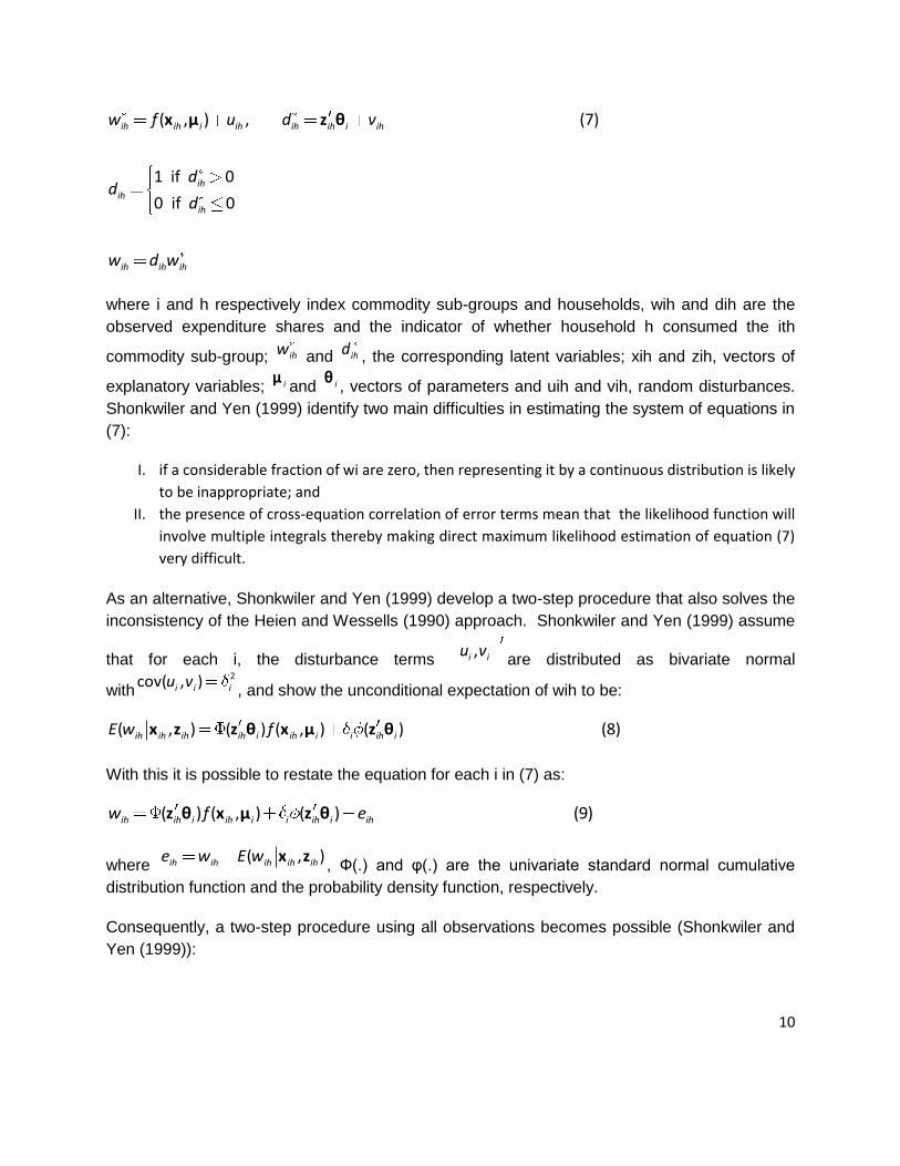
( , ) , (7)

1 if 0

0 if 0

ih ih i ih ih ih i ih

ihih

ih

ih ih ih

w f u d v

dd

d

w d w

x μ z θ

where i and h respectively index commodity sub-groups and households, wih and dih are the

observed expenditure shares and the indicator of whether household h consumed the ith

commodity sub-group; ihw and ihd , the corresponding latent variables; xih and zih, vectors of

explanatory variables; iμand iθ

, vectors of parameters and uih and vih, random disturbances.

Shonkwiler and Yen (1999) identify two main difficulties in estimating the system of equations in

(7):

I. if a considerable fraction of wi are zero, then representing it by a continuous distribution is likely

to be inappropriate; and

II. the presence of cross-equation correlation of error terms mean that the likelihood function will

involve multiple integrals thereby making direct maximum likelihood estimation of equation (7)

very difficult.

As an alternative, Shonkwiler and Yen (1999) develop a two-step procedure that also solves the

inconsistency of the Heien and Wessells (1990) approach. Shonkwiler and Yen (1999) assume

that for each i, the disturbance terms ,i iu v

are distributed as bivariate normal

with2cov( , )i i iu v, and show the unconditional expectation of wih to be:

( , ) ( ) ( , ) ( ) (8)ih ih ih ih i ih i i ih iE w fx z z θ x μ z θ

With this it is possible to restate the equation for each i in (7) as:

( ) ( , ) ( ) (9)ih ih i ih i i ih i ihw f ez θ x μ z θ

where ( , )ih ih ih ih ihe w E w x z

, Ф(.) and φ(.) are the univariate standard normal cumulative

distribution function and the probability density function, respectively.

Consequently, a two-step procedure using all observations becomes possible (Shonkwiler and

Yen (1999)):

11

Step 1: obtain ML probit estimates iθ of iθ using the binary outcome di = 1 and di = 0 for each

i;14

Step 2: calculate ( )iihz θ and ( )iihz θ and estimate 1 2, ,...μ μ and 1 2, ,... in the system

( ) ( , ) ( ) (10)i iih ih ih i i ih ihw fz θ x μ z θ

by ML or SUR procedure, where:

[ ( ) ( )] ( , ) [ ( ) ( )]i iih ih ih i ih ih i i ih i ihe fz θ z θ x μ z θ z θ

Three implications of this procedure should be noted:

The parameter estimates of the second step are consistent (Shonkwiler and Yen (1999)).

It is not possible to impose the adding-up condition via parametric restrictions as in the case of

the uncensored demand system (Drichoutis, et. al. (2008)). From the options available to

address this problem, the approach first recommended by Pudney (1989) and also recently

used, among others, by Yen, Lin, and Smallwood (2003) is adopted. The procedure involves

treating the nth good as a residual category and estimating the first n − 1 equations (i = 1, 2, . . . ,

n − 1) in the system (6), along with an identity: 1

1

1 (11)n

n ii

w w

defining the budget share of good n as a residual share. The adding-up identity can be used to

calculate elasticities of the residual good. However, the resulting estimates will not be invariant

to the good selected as the residual.

The disturbance terms in equation (10) are heteroscedastic. Steps to systematically deal with

this problem in line with ways suggested by Shonkwiler and Yen (1999) and Drichoutis, et. al.

(2008) were not attempted. Robust standard errors are used, however.

Endogeneity of total expenditure

The paper estimates a demand system spanning non-durables. The implicit assumption

underlying this partitioning is separability of durables and non-durables in household choice.

This creates the possibility that total expenditure is jointly determined with the budget shares of

the specific commodities in the demand model. In other words, total expenditure becomes

14

Shonkwiler and Yen (1999) acknowledge that “(e)stimation of the separate probit models implies the restriction E(vih ,vkh ) = 0 for i ≠ k, without which the multivariate probit model would have to be estimated. With some loss in efficiency (relative to multivariate probit) these separate probit estimates are nevertheless consistent.”

12

endogenous in the budget share equations – an endogeneity that may induce inconsistent

parameter estimates if not taken care of (Bundell and Robin (1999)). Bundell and Robin (1999)

recommend and illustrate an augmented regression technique to solve the problem. Two steps

are involved. First, total expenditure is regressed on a set of exogenous variables including

those which may directly influence budget shares. The residual from this reduced-form

regression is added, in the second step, as an explanatory variable in the budget share

equations together with total expenditure. The OLS estimator of the parameter of the total

expenditure variable in this augmented regression is identical to the Two-Stage Least Squares

(2SLS) estimator (Blundell and Robin (1999)). Moreover, Blundell and Robin (1999) argue that

testing for the significance of the coefficient, in the augmented regression, of the „residual‟

obtained in the first regression serves as a test of the exogeneity of total expenditure in the

share equations. The paper adopts this approach.

Spatial variation

As much as it is important to learn the national consumption responses to changes in prices and

income, it is imperative to recognize that the responsiveness of households may be different

across spatial locations. One important distinction of this type is between urban and rural areas.

Major differences in household characteristics, asset holdings and expenditure/income levels

between urban and rural households point towards potential differences in their reactions to

changes in economic variables (such as price and income). Accordingly, three sets of

elasticities were estimated: country-level (national) elasticities and elasticities for urban and

rural households separately.

Estimation – summary

The first step involved a probit regression to estimate the probability that a household will

consume the commodity under consideration. It expresses the dichotomous choice problem as: 1 1

0 1 2 3 4ln ln (12)R Z

ih ij j x h k kh l lh r r z z ij k l r z

d p x N a D D u

where dih=1 if the hth household consumes the ith food item, (i.e., if wih > 0) and 0 if the

household does not consume the item in question; Nks are household demographic variables

(household size, age of household head, age of household age squared, gender of household

head, and years of schooling completed by the household head), ajs are household assets

(household ownership of its dwelling unit, number of rooms in the dwelling unit, main

construction material of the dwelling‟s roof, number of dwellings/other buildings owned by the

household, number of pack animals owned, number of gas or electric stove owned, number of

radios owned, number of plough animals owned, and number of bicycles owned ), Drs are

regional dummies (10 regions), Dzs are zonal dummies (74 zones). The zero-expenditure

problem happened to be significant in size for sorghum (28 percent), teff (22 percent), maize (16

13

percent), wheat (9 percent), and, marginally, animal products (2 percent). Equation (12) was

estimated for all commodities. The corresponding ( )iihz θ and ( )iihz θ are computed from

these regressions and subsequently entered in the second-stage estimation as instruments that

correct for the zeros in the dependent variable.

Prior to executing the second-stage, total expenditure was regressed on its determinants:

1 1

0 1 2 3 4ln ln (13)R Z

h ij j k hk l hl r r z z hj k l r z

x p N a D D e

where, xh is total household consumption expenditure on non-durables, Nks are household

demographic variables (household size, age of household head, gender of household head, and

years of schooling completed by the household head), ajs are household assets (household

ownership of its dwelling unit, number of rooms in the dwelling unit, main construction material

of the dwelling‟s roof, type of toilet facility of the household, number of dwellings/other buildings

owned by the household, number of pack animals owned, number of gas or electric stove

owned, number of radios owned, number of plough animals owned, number of equine animals,

number of sheep and goats owned, number of equine animals owned, and number of bicycles

owned), Drs are regional dummies (10 regions), Dzs are zonal dummies (74 zones), and e is a

normally distributed residual. The residuals he are computed and subsequently entered in the

budget share equations estimated in the second-stage.

Therefore, the demand system finally estimated takes the form:15

2

1

( ) ln ln ln + ( ) (14)( ) ( ) ( )

nh i h

i iih ih i ij j i i h i ih ih

j

x xw p e

a b az θ z θ

p p p

where he is the residual from the total expenditure regression and( )iihz θ

and ( )iihz θ

are

obtained from the first-stage probit regressions.

The parameters of the QU-AIDM model is estimated using Poi‟s STATA routine (Poi, 2008) after

modifying it to include additional control variables in order to capture endogeneity and selectivity

problems as appropriate.16

15

See Appendix III for price and expenditure elasticity of demand formulas under QU-AIDM model. 16

The authors would like to thank Miguel Robles of IFPRI for providing them with his modified STATA ado and do files which served as a basis for subsequent adaptation.

14

The specific estimation technique chosen reflects a number of requirements in part created by

the specific features of the QU-AIDM. First, adding-up, homogeneity, and symmetry have to be

accommodated. The adding-up condition is accommodated by dropping one of the budget

share equations and imposing an adding-up identity (see above). Symmetry and homogeneity,

on the other hand, have to be explicitly imposed during estimation. The way this is achieved

reflects the nature of these restrictions. Symmetry is a cross-equation restriction, whereas

homogeneity is essentially a within-equation restriction. The joint application of the two is a

major feature of the QU-AIDM. Second, QU-AIDM is non-linear because of the quadratic total

expenditure term and the two expressions in log prices (a(p) and b(p)). To handle these features

the model was estimated as a non-linear system of seemingly unrelated regression equations

(or NSURE).17 Parameter estimates were thus obtained by estimating the respective system of

SURE, with symmetry and homogeneity simultaneously imposed. In each case the „Other non-

food‟ budget-share equation is dropped to accommodate adding-up. The remaining 20

equations were estimated by iterated feasible generalised non-linear least squares (IFGNLS)

which is equivalent to the maximum likelihood (ML) (Poi (2008)).18,19 Estimates of the elasticities

of the excluded (or dropped) budget-share equation are then recovered by exploiting the

adding-up and homogeneity restrictions.20

17

The NSURE framework also accommodates the possibility that the disturbances contain unobserved factors common to budget shares. 18

All estimation procedures were implemented using Stata/MP 11.0 for Windows .

19 Following the recommendation in Deaton and Muellbauer (1980a) 0 in ln ( )ap is chosen to be just below the lowest value of lnx

in the data. This ensures positive real total expenditure throughout. Note also that a number of 20

For uncensored versions of the model estimates, the parameters of the of the excluded (or dropped) budget-share equation are recovered by exploiting the adding-up and homogeneity restrictions, with their standard errors computed via the delta method.

15

5. RESULTS

Tables 8.1-8.3 report the parameter estimates of the QU-AIDM obtained at the country-level and

for rural areas and urban areas, respectively.

Country-Level Results

The overall performance of the QU-AIDM at the country level can be ascertained with the

information in Table 9.1. The root mean square error (RMSE) of each of the budget share

equation is low. Ranging from 0.11 through to 0.82, with half of them greater than 0.5, the

corresponding R2 values are credible. Consistent with these is the statistical significance of

most of the unrestricted coefficients (268 out of 310, to be specific) reported in the Table 9.1.

Moreover, the probability density term turned out significant in all the equations but one thereby

further corroborating the importance of adjusting for zero-expenditures. The services group

proved the exception – an expected result in light of the fact that this group has the highest

budget share and no reported zero expenditure (0.02 percent to be exact).

Total expenditure and prices are shown to be significant determinants of demand. Looking at

the results for expenditure first, the exogeneity of total expenditure is rejected for all

commodities except barley, the enset group, and clothing and shoes.21 Controlling for its

endogeneity, total expenditure turns out to be highly significant, both linearly and quadratically,

in the budget share equations. Maize, pulses, and sugar and salt proved to be the exception. As

to prices, most come out significant. Out of the possible 230 distinct price effects only 26 are

insignificant – eight of these being in the teff share equation and seven in that of oil seeds.

Substantively more informative and significant are the price and expenditure elasticity

estimates. Country-level elasticity estimates are reported in Tables 1, 2, and 3. The

compensated own-price elasticities are, as predicted by theory, negative for all commodities.22

That they are also close to -1 suggests that most of the commodities are own-price unitary

elastic. Own-price elasticities of maize and sorghum are the furthest away from -1.

Cross-price effects are also present, although they appear rather weak for most commodity

pairs (Tables 1b, 4, and 5). Among the four major cereal items (teff, wheat, maize, and

sorghum) complementarity is detected between the teff-sorghum and maize-sorghum pairs,

while substitution appears to be the link between teff and wheat. These results seem to reflect

21

Recall that the relevant check is the t-test of the significance of the residual term that enters each budget share equation from the reduced–form regression using equation (13) above. The results of the reduced-form estimation can be found in Table 11 (add the table). 22

The only exception is the residual „other non-food‟ group whose elasticity is computed using the estimates of the rest of the commodity groups using adding-up and homogeneity.

16

limited possibilities in consumption for substitution and/or complementarity in Ethiopia. Diversity

in the bio-physical and socio-economic landscape are likely to constrain these possibilities.

Table 1a: Compensated Price Elasticities (Country-level)23

National

Teff -0.888

Wheat -0.981

Barley -0.948

Maize -0.746

Sorghum -0.656

Other cereals -1.074

Processed Cereals -1.022

Pulses -0.952

Oilseeds -0.999

Animal products -0.939

Oils and Fats -0.983

Vegetables and Fruits -0.979

Pepper -0.991

Enset/Kocho/Bula -0.993

Coffee/Tea/Chat -0.960

Root crops -0.985

Sugar and Salt -0.989

Other foods -0.976

Clothing and Shoes -0.953

Services -0.683

Other Non-food 0.873

Source: Authors‟ calculation based on CSA‟s HICE 2004/05 data.

The expenditure elasticity estimates indicate that most commodities are normal, though some

are marginally so (Table 2). The negative expenditure elasticities of „other cereals‟ and barley

indicate that the two are inferior. For the former, which is dominated by millet, the result is

clearly driven by the outcome in urban demand. Teff, other cereals, processed cereals, pulses,

animal products, and services have income elastic demands. These results are consistent with

the perception that teff and animal products are generally considered superior food types in the

country. On the other hand, wheat, maize, and sorghum, appear as expenditure-inelastic. That

maize and sorghum are relatively less desired cereals in most parts of the country, while a

significant fraction of wheat originates as food aid may be the explanations.

23

For the full elasticity estimates (both national and urban/rural) see Tables 4-7.

17

Table 1b: Compensated Price Elasticities of Cereals (National)

QU-AIDM

Teff Wheat Barley Maize Sorghum

Teff -0.89 0.10 0.06 0.05 -0.10

Wheat 0.06 -0.98 0.05 0.04 0.05

Barley -0.02 0.00 -0.95 -0.02 -0.04

Maize 0.04 0.05 0.04 -0.75 -0.05

Sorghum -0.03 0.04 0.02 -0.07 -0.66 Source: Authors‟ calculation based on CSA‟s HICE 2004/05 data.

A number of studies report price and expenditure elasticities of demand estimated form

Ethiopian datasets. These include Kedir (2005), Taffesse (2003), and Shimeles (1993). Table 7

reports the estimates of these studies alongside with those of the current paper. Kedir (2005)

uses data from the Ethiopian Urban Household Survey, while Taffesse (2003) the Ethiopian

Rural Household Survey (ERHS)-1994. In contrast, Shimeles (1993) is based on aggregated

CSA data. In addition to some matched ones, a number of their elasticity estimates have

imperfect analogues in the present paper. The values in Table 7 reveal that the estimates in

Taffesse (2003) and Shimeles (1993) are broadly similar to the current paper‟s, while those of

Kedir (2005) are rather divergent.

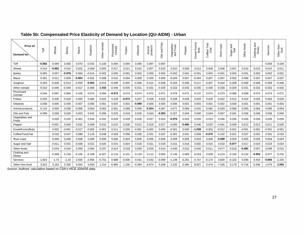
Rural and Urban Area Results

As noted earlier, the QU-AIDM was fitted to the rural and urban segments of the HICES sample

separately. The objective is to ascertain the extent to which demand responses vary between

the two household groupings. A number of significant differences are uncovered (Tables 2 and

5). Expenditure elasticities of sorghum, pulses, and the enset group are higher in rural areas.

„Other cereals‟, „oil seeds‟, and „sugar and salt.‟ Have higher expenditure elasticites in urban

areas. More varied, and sometimes stronger, cross-price effects were detected within each sub-

sample as well as between the samples. In contrast, own-price elasticities came out more or

less the same.

18

Table 2: Expenditure Shares and Expenditure Elasticities

Expenditure Share (%) Expenditure Elasticity of Demand (QU-AIDM)

National Rural Urban National Rural Urban

Teff 4.96 4.37 8.17 1.69 1.08 1.14

Wheat 5.06 5.53 2.57 0.78 0.42 0.41

Barley 2.55 2.91 0.57 -0.44 0.06 0.33

Maize 4.97 5.67 1.15 0.92 0.62 0.58

Sorghum 4.71 5.39 1.05 0.77 1.00 -0.81

Other cereals 0.89 0.97 0.47 -6.70 2.30 -6.70

Processed Cereals 1.91 0.96 7.00 2.33 -1.29 1.04

Pulses 4.47 4.73 3.06 1.03 1.13 0.87

Oilseeds 0.13 0.14 0.04 0.63 0.96 2.10

Animal products 4.43 4.28 5.22 1.31 1.22 1.23

Oils and Fats 1.95 1.56 4.03 0.72 0.83 0.90

Vegetables and Fruits 2.57 2.49 2.98 0.87 0.95 0.87

Pepper 1.53 1.49 1.74 0.41 0.30 0.67

Enset/Kocho/Bula 2.25 2.61 0.28 0.87 2.12 -0.39

Coffee/Tea/Chat 5.54 5.87 3.75 0.88 1.39 0.85

Root crops 1.85 2.03 0.91 0.94 0.18 0.59

Sugar and Salt 1.05 0.89 1.93 0.79 0.16 0.96

Other foods 5.92 5.85 6.30 0.16 0.52 0.12

Clothing and Shoes 6.50 6.28 7.70 0.74 1.19 0.67

Services 22.40 21.56 26.95 1.45 0.86 1.35

Other Non-food 14.37 14.41 14.14 1.38 1.72 1.50

Source: Authors‟ calculation based on CSA‟s HICE 2004/05 data.

Expenditure elasticity estimates point out that most consumption items are normal goods (see

Table 2). The QU-AIDM model indicates that teff, other cereals, processed cereals, and animal

products have elastic demand in both urban and rural areas. This finding further supports the

claims made above about the public perception of the items. It is also interesting to find

processed cereals (in rural areas) and other cereals (in rural areas) appear to be inferior goods.

19

Table 3: Price Elasticities of Cereals (Urban/Rural)

Teff Wheat Barley Maize Sorghum

Ru

ral

Teff -0.905 0.051 0.04 0.03 -0.077

Wheat 0.027 -0.978 0.028 0.034 0.022

Barley -0.003 0.009 -0.976 0.003 -0.009

Maize 0.031 0.043 0.037 -0.873 0.001

Sorghum 0.007 0.053 0.048 0.012 -0.84

Urb

an

Teff -0.862 0.094 0.083 0.07 -0.042

Wheat 0.013 -0.992 0.015 0.022 0.008

Barley -0.005 0.007 -0.978 0 -0.014

Maize 0.001 0.011 0.006 -0.904 -0.031

Sorghum -0.053 -0.009 -0.014 -0.05 -0.902

Source: Authors‟ calculation based on CSA‟s HICE 2004/05 data.

20

6. CONCLUSIONS

This paper is aims at empirically investigating the responsiveness of demand for various food

and non-food items to changes in price and expenditure using the Quadratic Linear Almost Ideal

Demand Model (AIDM). The demand system was estimated using non-linear Seemingly

Unrelated Regression (NSURE) technique using Household Income Consumption Expenditure

Survey 2004/05 data collected by Central Statistical Agency of Ethiopia. Zero expenditures were

accommodated via censored regression.

The findings of the study suggest that Ethiopian households display significant response to

changes in prices and expenditure/income. It is interesting to note that price elasticities of

demand for cereals are roughly the same in urban and rural areas of the country.

21

REFERENCES

Banks, J., R. W. Blundell, and A. Lewbel (1997). “Quadratic Engel curves, welfare measurement

and consumer demand,” Review of' Economics and Statistics, LXXIX(4), 527-539.

Blundell, Richard, and Jean Marc Robin (1999). “Estimation in Large and Disaggregated

Demand Systems: An Estimator for Conditionally Linear Systems,” Journal of Applied

Econometrics, Vol. 14, No. 3, pp. 209-232.

Browning, Martin, Pierre-André Chiappori, and Valérie Lechene (2006). “Collective and Unitary

Models: A Clarification,” Review of Economics of the Household, 4, pp. 5–14.

Capéau, Bart, Stefan Dercon (2005). “Prices, Unit Values and Local Measurement Units in

Rural Surveys: an Econometric Approach with an Application to Poverty Measurement in

Ethiopia,” Journal of African Economies, Volume 15, Number 2, pp. 181–211.

Crawford, Ian, François Laisney, and Ian Preston (2003). “Estimation of household demand

systems with theoretically compatible Engel curves and unit value specifications,” Journal of

Econometrics, 114, pp. 221–241.

CSA (June 2004). Welfare Monitoring Survey 2004 - Analytical Report, Central Statistical

Authority (CSA), Addis Ababa, Ethiopia.

CSA (May 2007). “Household Income, Consumption and Expenditure (HICE) Survey 2004/5:

Volume I - Analytical Report,” Statistical Bulletin 394, Central Statistical Authority (CSA), Addis

Ababa, Ethiopia.

Deaton, Angus S. (1997). The Analysis of Household Surveys: A Microeconometric Approach to

Development Policy. John Hopkins University Press for the World Bank, Baltimore.

______, (1990). “Price Elasticities from Survey Data: Extensions and Indonesian Results,”

Journal of Econometrics , 44, 281-309.

______, (1988). “Quality, Quantity, and Spatial Variation of Price,” American Economic Review ,

78 (3), 418-430.

______, (1987). “Estimation of Own- and Cross-Price Elasticities from Household Survey Data,”

Journal of Econometrics , 36, 7-30.

Deaton, Angus S., and John Muellbauer (1980a). “An Almost Ideal Demand System,” American

Economic Review , 70 (3), 312-326.

22

______, and _____ (1980b). Economics and Consumer Behaviour. Cambridge University

Press.

Drichoutis, Andreas C., Stathis Klonaris, Panagiotis Lazaridis, and Rodolfo M. Nayga, Jr.

(2008). “Household food consumption in Turkey: a comment,” European Review of Agricultural

Economics, pp. 1–6.

Heien, Dale and Cathy Roheim Wessells (1990). “Demand Systems Estimation With Microdata:

A Censored Regression Approach,” Journal of Business and Economic Statistics , 8 (3), 365-

371.

Kedir, Abbi M. (2001). “Some Issues in Using Unit Values as Prices in the Estimation of Own-

Price Elasticities: Evidence from Urban Ethiopia,” CREDIT Research Paper .

______, (2005). “Estimation of Own and Cross-price Elasticities using Unit Values: Econometric

Issues and Evidence from Urban Ethiopia,” Journal of African Economies , 14 (1), 1-20.

Moschini, G. (1995). “Units of Measurement and the Stone Index in Demand System

Estimation,” American Journal of Agricultural Economics , 77, 63-68.

Poi, B. P. (2008). “Demand System Estimation: Update,” The Stata Journal , 2 (4), 554-556.

Shimeles, Abebe (1993). “System of Demand Equations: Theory and Applications,” Ethiopian

Journal of Economics , II (2), 1-54.

Shonkwiler, J. S., and Yen, S.T. (November 1999). “Two-Step Estimation of a Censored System

of Equations,” American Journal of Agricultural Economics, Volume 81, No. 4, pp. 972-982.

Taffesse, Alemayehu Seyoum (2003). “Rationed Consumer Demands: An Applicaiton to the

Demand for Food in Rural Ethiopia,” PHOTOCOPIED.

TEFERA, NIGUSSIE (AUGUST 2009). “Household Demand for Food Consumption in Rural

Ethiopia: Two-Step Estimation of a Censored Demand System,” PHOTOCOPIED.

TEFERA, NIGUSSIE, SHAIDUR RASHID, ALEMAYEHU SEYOUM TAFFESSE (AUGUST 2009). “WELFARE

IMPLICATIONS OF RISING CEREALS PRICES IN RURAL ETHIOPIA: A NON-PARAMETRIC ANALYSIS,”

PHOTOCOPIED.

Ulimwengu, John M., Sindu Workneh, and Zelekawork Paulos (February 2009). “Impact of

Soaring Food Price in Ethiopia - Does Location Matter?” IFPRI Discussion Paper 00846,

International Food Policy Research Institute (IFPRI).

23

Yen, Steven T., Biing-Hwan Lin, and David M. Smallwood (2003). “Quasi- and simulated-

likelihood approaches to censored demand systems: food consumption by food stamp

recipients in the United States,” American Journal of Agricultural Economics, 85, pp. 458–478.

Yen, Steven T., and Biing-Hwan Lin (August 2006). “A Sample Selection Approach to Censored

Demand Systems,” American Journal Agricultural Economics, 88, 3, Pp. 742–749

24

Table 1 Consumption and sociodemographic variables definitions

Table 4: Compensated Price Elasticity of Demand (QU-AIDM) – Country-level

Price of:

Demand for:

Teff

Whea

t

Barley

Maiz

e

Sorg

hu

m

Oth

er

cere

als

Pro

ce

sse

d C

ere

als

Puls

es

Oils

ee

ds

Anim

al pro

ducts

Oils

and F

ats

Vegeta

ble

s a

nd

F

ruits

Pepp

er

Enset/

Kocho

/ B

ula

Coffe

e/

Te

a/ C

hat

Root

cro

ps

Suga

r a

nd S

alt

Oth

er

foo

ds

Clo

thin

g a

nd S

hoes

Serv

ices

Oth

er

Non

-fo

od

Teff -

0.888 0.104 0.062 0.048

-0.102

0.104 0.063 0.093 0.081 0.094 0.077 . . . . . . . . 0.083 0.104

Wheat 0.058 -

0.981 0.048 0.039 0.050 0.019 0.049 0.041 0.040 0.035 0.039 0.035 0.037 0.131 0.032 0.011 0.032 0.035 0.040 0.039 0.039

Barley -

0.023 0.002

-0.948

-0.022

-0.044

-0.014

-0.004

-0.015

-0.010

-0.015

-0.011

-0.013

-0.013

-0.075

-0.010

-0.015

-0.014

-0.015

-0.012

-0.011

-0.011

Maize 0.037 0.045 0.040 -

0.746 -

0.051 0.045 0.044 0.043 0.044 0.042 0.045 0.035 0.045

-0.013

0.046 0.045 0.035 0.045 0.045 0.046 0.044

Sorghum -

0.028 0.043 0.021

-0.071

-0.656

0.021 0.035 0.045 0.037 0.033 0.036 0.037 0.036 -

0.068 0.039 0.004 0.031 0.036 0.036 0.036 0.036

Other cereals -

0.027 -

0.095 -

0.065 -

0.060 -

0.109 -

1.074 -

0.053 -

0.061 -

0.058 -

0.054 -

0.057 -

0.057 -

0.062 -

0.117 -

0.059 -

0.065 -

0.061 -

0.061 -

0.060 -

0.060 -

0.061

Processed Cereals -

0.021 0.092 0.069 0.028 0.029 0.062

-1.022

0.036 0.045 0.051 0.042 0.039 0.041 0.285 0.044 0.034 0.045 0.038 0.044 0.045 0.037

Pulses 0.074 0.050 0.034 0.032 0.091 0.043 0.042 -

0.952 0.046 0.047 0.045 0.043 0.045 0.009 0.049

-0.046

0.016 0.041 0.046 0.046 0.043

Oilseeds 0.003 0.001 0.000 -

0.008 0.005 0.002 0.002 0.001

-0.999

0.001 0.001 0.000 0.000 0.006 0.002 -

0.004 0.000 0.001 0.001 0.001 0.004

Animal products 0.164 -

0.008 0.009

-0.057

-0.041

0.095 0.074 0.060 0.056 -

0.939 0.061 0.065 0.069

-0.083

0.055 0.001 0.073 0.054 0.058 0.058 0.036

Oils and Fats -

0.192 -

0.020 0.003

-0.003

0.000 0.081 -

0.006 0.001 0.010 0.028

-0.983

-0.052

0.030 0.147 0.047 0.069 0.023 0.014 0.013 0.013 0.050

Vegetables and Fruits

. 0.024 0.026 0.009 0.031 0.028 0.024 0.025 0.022 0.023 0.021 -

0.979 0.022 0.012 0.020 0.040 0.024 0.022 0.022 0.022 0.023

Pepper . -

0.014 -

0.002 0.049 0.060 0.002 0.005 0.016 0.005 0.030 0.015 0.007

-0.991

0.121 0.022 -

0.029 0.001 0.007 0.006 0.008

-0.073

Enset/Kocho/Bula . 0.038 0.014 0.003 -

0.009 0.016 0.028 0.019 0.020 0.018 0.020 0.018 0.020

-0.993

0.019 0.020 0.025 0.019 0.020 0.020 0.023

Coffee/Tea/Chat . -

0.059 0.087 0.112 0.173 0.080 0.060 0.085 0.057 0.047 0.061 0.010 0.060 0.023

-0.960

0.085 0.020 0.045 0.048 0.049 0.003

Root crops . 0.015 0.019 0.021 0.010 0.019 0.018 0.013 0.017 0.017 0.018 0.021 0.017 0.017 0.018 -

0.985 0.018 0.017 0.017 0.018 0.016

Sugar and Salt . 0.005 0.011 -

0.016 0.002 0.013 0.012

-0.003

0.008 0.010 0.009 0.011 0.008 0.059 0.006 0.014 -

0.989 0.008 0.008 0.008 0.011

25

Other foods . 0.012 0.028 0.079 0.094 0.049 0.020 0.025 0.034 0.019 0.015 0.051 0.018 0.076 0.016 0.110 0.039 -

0.976 0.009 0.012 0.046

Clothing and Shoes

. 0.367 0.052 -

0.155 -

0.413 0.001 0.031 0.060 0.074 0.094 0.043 0.059 0.046 0.170 0.036 0.207 0.064

-0.084

-0.953

0.063 0.214

Services 0.344 0.350 0.225 0.197 -

0.265 0.452 0.626 0.382 0.201 0.479 0.251 0.205 0.578 0.176 0.306 4.714 0.402 0.809 0.390

-0.683

-0.706

Other Non-food -

0.290 -

0.440 -

0.340 -

0.060 0.730

-0.830

-0.990

-0.470

-0.490

-0.630

-0.42 -

0.270 -

0.940 -

0.290 -

0.220 -7.41 -0.68 -0.92

-0.290

0.900 0.873

Source: Authors‟ calculation based on CSA‟s HICE 2004/05 data

26

.

Table 5a: Compensated Price Elasticity of Demand by Location (QU-AIDM) - Rural Price of:

Demand for:

Teff

Whea

t

Barle

y

Maiz

e

Sorg

h

um

Oth

er

cere

a

ls

Pro

ce

ssed

Cere

als

Puls

e

s

Oils

e

eds

Anim al

pro

du

cts

Oils

and

Fats

Veget

able

s

and

Fru

its

Pepp

er

Enset

/

Koch

o/

Bula

C

offe

e/

Te

a/

Chat

Root

cro

ps

Suga

r

and

Salt

Oth

er

foo

ds

Clo

thi

ng

and

Shoe

s

Serv

i

ces

Oth

er

Non-

foo

d

Teff -

0.905 0.051 0.040 0.030

-0.077

0.060 0.040 0.050 0.051 0.052 0.043 . . . . . . . . 0.047 0.071

Wheat 0.027 -

0.978 0.028 0.034 0.022 0.017 0.029 0.024 0.023 0.020 0.023 0.025 0.023 0.036 0.022 0.028 0.020 0.023 0.023 0.023 0.025

Barley -

0.003 0.009

-0.976

0.003 -

0.009 -

0.002 0.006 0.000 0.003 0.001 0.002 0.001 0.001 0.004 0.003 0.006 0.008 0.001 0.002 0.002 0.002

Maize 0.031 0.043 0.037 -

0.873 0.001 0.040 0.039 0.033 0.035 0.034 0.035 0.023 0.035 0.011 0.036 0.040 0.027 0.035 0.035 0.035 0.036

Sorghum 0.007 0.053 0.048 0.012 -

0.840 0.046 0.054 0.062 0.055 0.052 0.054 0.063 0.054 0.053 0.056 0.064 0.055 0.054 0.054 0.054 0.055

Other cereals 0.037 0.012 0.016 0.032 0.001 -

0.979 0.017 0.020 0.023 0.023 0.023 0.033 0.022 0.027 0.024 0.033 0.028 0.024 0.022 0.022 0.023

Processed Cereals -

0.041 0.017 0.001 0.022

-0.008

-0.033

-1.056

-0.010

-0.010

-0.013

-0.014

0.002 -

0.013 0.194

-0.013

0.004 -

0.020 -

0.016 -

0.013 -

0.011 -

0.014

Pulses 0.059 0.054 0.046 0.032 0.096 0.047 0.054 -

0.946 0.054 0.055 0.052 0.060 0.056 0.064 0.058 0.021 0.034 0.052 0.053 0.053 0.054

Oilseeds 0.008 0.000 0.001 -

0.006 0.005 0.002 0.003 0.002

-0.998

0.001 0.001 0.000 0.001 0.008 0.002 -

0.001 0.000 0.001 0.001 0.002

-0.007

Animal products 0.090 0.001 0.029 -

0.001 0.006 0.050 0.049 0.055 0.047

-0.947

0.054 0.057 0.056 -

0.021 0.050

-0.033

0.059 0.051 0.052 0.054 0.036

Oils and Fats -

0.149 0.013 0.005

-0.025

0.019 0.048 0.000 -

0.012 0.002 0.023

-0.986

-0.075

0.022 0.207 0.024 0.053 0.025 0.013 0.013 0.012 0.087

Vegetables and Fruits

. 0.025 0.023 0.001 0.039 0.030 0.026 0.026 0.023 0.024 0.022 -

0.978 0.023 0.025 0.022 0.043 0.025 0.023 0.024 0.024 0.024

Pepper . -

0.007 -

0.005 0.028 0.004 0.003 0.004 0.027 0.006 0.015 0.009

-0.013

-0.992

0.112 0.016 -

0.048 0.000 0.006 0.004 0.004

-0.010

Enset/Kocho/Bula . 0.056 0.055 0.049 0.054 0.055 0.059 0.055 0.055 0.055 0.056 0.055 0.056 -

0.953 0.055 0.050 0.055 0.055 0.055 0.055 0.057

Coffee/Tea/Chat . 0.065 0.092 0.129 0.146 0.099 0.078 0.107 0.083 0.080 0.085 0.048 0.089 0.022 -

0.920 0.138 0.060 0.076 0.081 0.081 0.059

Root crops . 0.005 0.005 0.007 0.008 0.005 0.005 0.002 0.004 0.003 0.004 0.008 0.003 -

0.001 0.004

-0.999

0.004 0.004 0.004 0.004 -

0.001

Sugar and Salt . -

0.002 0.008

-0.019

0.003 0.006 0.000 -

0.007 0.001 0.003 0.002 0.003 0.001 0.004 0.000 0.002

-0.994

0.001 0.001 0.002 0.007

Other foods . 0.064 0.056 0.074 0.075 0.069 0.037 0.042 0.049 0.040 0.035 0.060 0.037 0.117 0.034 0.099 0.051 -

0.958 0.029 0.033 0.045

Clothing and Shoes

. 0.121 0.023 -

0.135 -

0.163 -

0.059 -

0.038 0.043 0.055 0.082 0.065 0.021 0.062

-0.263

0.038 -

0.072 0.030

-0.054

-0.934

0.093 0.215

Services 0.819 1.160 1.183 1.641 1.440 1.090 1.327 0.846 1.271 0.873 0.282 1.532 0.327 -

1.020 0.352 7.445 1.691 0.964 0.327

-0.801

-0.976

Other Non-food -

1.005 -

1.554 -

1.738 -

2.185 -

1.895 -

1.714 -

2.054 -

1.128 -

2.076 -

1.202 -

0.498 -

2.258 -

0.561 1.649

-0.280

-11.13

-2.614

-1.154

-0.221

1.003 1.206

Source: Authors‟ calculation based on CSA‟s HICE 2004/05 data.

27

Table 5b: Compensated Price Elasticity of Demand by Location (QU-AIDM) - Urban

Price of:

Demand for:

Teff

Whea

t

Barley

Maiz

e

Sorg

hu

m

Oth

er

cere

als

Pro

ce

sse

d

Cere

als

Puls

es

Oils

ee

ds

Anim

al

pro

ducts

Oils

and F

ats

Vegeta

ble

s

and

Fru

its

Pepp

er

Enset/

Kocho/

Bula

Coffe

e/

Te

a/

Chat

Root

cro

ps

Suga

r a

nd

Salt

Oth

er

foo

ds

Clo

thin

g a

nd

Shoes

Serv

ices

Oth

er

Non

-

foo

d

Teff -0.862 0.094 0.083 0.070 -0.042 0.100 0.084 0.094 0.095 0.097 0.087 . . . . . . . . 0.093 0.104

Wheat 0.013 -0.992 0.015 0.022 0.008 0.005 0.017 0.011 0.010 0.007 0.010 0.010 0.009 0.012 0.009 0.008 0.007 0.010 0.010 0.010 0.011

Barley -0.005 0.007 -0.978 0.000 -0.014 -0.002 0.005 -0.001 0.002 0.000 0.002 -0.002 0.001 -0.001 0.002 -0.001 0.004 0.001 0.002 0.002 0.002

Maize 0.001 0.011 0.006 -0.904 -0.031 0.008 0.010 0.004 0.006 0.005 0.006 -0.004 0.007 -0.004 0.007 0.007 0.002 0.006 0.007 0.007 0.007

Sorghum -0.053 -0.009 -0.014 -0.050 -0.902 -0.013 -0.008 -0.002 -0.008 -0.010 -0.008 -0.003 -0.009 -0.011 -0.007 -0.004 -0.009 -0.009 -0.009 -0.009 -0.008

Other cereals -0.010 -0.046 -0.040 -0.017 -0.066 -1.033 -0.040 -0.035 -0.031 -0.031 -0.029 -0.023 -0.033 -0.035 -0.030 -0.028 -0.029 -0.031 -0.032 -0.032 -0.032

Processed Cereals

0.044 0.097 0.084 0.105 0.074 0.059 -0.972 0.073 0.074 0.072 0.071 0.079 0.071 0.137 0.071 0.073 0.066 0.069 0.072 0.073 0.071

Pulses 0.033 0.028 0.018 0.000 0.082 0.022 0.028 -0.973 0.027 0.028 0.025 0.028 0.028 0.025 0.030 -0.022 0.012 0.024 0.026 0.026 0.026

Oilseeds 0.008 0.000 0.000 -0.007 0.005 0.001 0.002 0.001 -0.998 0.000 0.000 0.000 0.001 0.003 0.001 -0.002 0.000 0.001 0.001 0.001 -0.003

Animal products 0.115 0.004 0.038 -0.006 0.004 0.063 0.061 0.068 0.058 -0.934 0.067 0.071 0.069 0.032 0.062 -0.033 0.069 0.063 0.064 0.065 0.054

Oils and Fats -0.099 0.036 0.030 0.003 0.042 0.056 0.025 0.019 0.028 0.043 -0.963 -0.027 0.044 0.095 0.044 0.067 0.041 0.036 0.036 0.036 0.065

Vegetables and Fruits

. 0.028 0.025 -0.001 0.044 0.031 0.029 0.028 0.026 0.027 0.024 -0.976 0.025 0.026 0.024 0.046 0.026 0.026 0.026 0.026 0.026

Pepper . -0.001 0.000 0.031 0.008 0.010 0.010 0.028 0.012 0.019 0.017 -0.005 -0.985 0.046 0.020 -0.041 0.009 0.012 0.012 0.011 0.005

Enset/Kocho/Bula . 0.002 -0.001 -0.017 -0.002 -0.001 0.011 0.000 -0.001 -0.002 0.000 -0.001 0.000 -1.008 -0.002 -0.012 -0.001 -0.001 -0.001 -0.001 0.001

Coffee/Tea/Chat . 0.016 0.047 0.098 0.119 0.048 0.029 0.058 0.035 0.031 0.037 -0.001 0.041 0.009 -0.970 0.102 0.021 0.027 0.031 0.031 0.019

Root crops . 0.006 0.006 0.008 0.009 0.006 0.006 0.004 0.005 0.005 0.006 0.009 0.005 0.003 0.006 -0.999 0.005 0.005 0.005 0.006 0.003

Sugar and Salt . 0.011 0.031 -0.028 0.021 0.025 0.015 0.004 0.018 0.021 0.019 0.021 0.018 0.020 0.016 0.018 -0.977 0.017 0.019 0.019 0.024

Other foods . 0.043 0.034 0.059 0.060 0.037 0.014 0.018 0.028 0.016 0.014 0.036 0.015 0.042 0.011 0.077 0.018 -0.982 0.007 0.009 0.015

Clothing and Shoes

. 0.348 0.128 -0.105 -0.189 -0.027 -0.110 0.101 0.129 0.112 0.064 0.145 0.069 0.019 0.028 0.223 0.100 -0.132 -0.952 0.077 0.232

Services -1.815 -1.74 -1.33 -2.926 -2.956 -0.701 0.688 -0.606 0.031 0.432 -0.090 -1.148 -0.201 -4.757 -0.170 3.600 -0.102 0.595 0.403 -0.666 -1.235

Other Non-food 3.915 3.163 2.350 5.564 5.693 1.214 -0.880 1.155 -0.284 -0.674 0.269 2.232 0.360 8.927 0.474 -7.026 0.179 -0.716 -0.346 1.073 2.065

Source: Authors‟ calculation based on CSA‟s HICE 2004/05 data.

28

Table 6: Summary of Own Price Elasticities (QU-AIDM)

National Rural Urban

Teff -0.888 -0.905 -0.862

Wheat -0.981 -0.978 -0.992

Barley -0.948 -0.976 -0.978

Maize -0.746 -0.873 -0.904

Sorghum -0.656 -0.840 -0.902

Other cereals -1.074 -0.979 -1.033

Processed Cereals -1.022 -1.056 -0.972

Pulses -0.952 -0.946 -0.973

Oilseeds -0.999 -0.998 -0.998

Animal products -0.939 -0.947 -0.934

Oils and Fats -0.983 -0.986 -0.963

Vegetables and Fruits -0.979 -0.978 -0.976

Pepper -0.991 -0.992 -0.985

Enset/Kocho/Bula -0.993 -0.953 -1.008

Coffee/Tea/Chat -0.960 -0.920 -0.970

Root crops -0.985 -0.999 -0.999

Sugar and Salt -0.989 -0.994 -0.977

Other foods -0.976 -0.958 -0.982

Clothing and Shoes -0.953 -0.934 -0.952

Services -0.683 -0.801 -0.666

Other Non-food 0.873 1.206 2.065

Source: Authors‟ calculation based on CSA‟s HICE 2004/05 data

29

Table 7: Comparison of Own Price Elasticity of Demand Estimates

Te

ff

Wh

ea

t

Ma

ize

So

rgh

um

Oth

er

Ce

rea

ls

Pu

lse

s

An

ima

l

Pro

du

cts

Fru

its

an

d

Ve

ge

tab

les

Ro

ot

cro

ps

Gra

in

Ce

rea

ls

Fo

od

QAIDM

National -0.888

-0.981 -0.746

-0.656

-1.074

-0.952 -0.939

-0.979 -0.985

Rural -0.905

-0.978 -0.873

-0.840

-0.979

-0946 -0.947

-0.978 -0.999

Urban -0.862 -0.992

-0.904

-0.902

-1.033

-0.973 -0.934 -0.976 -0.999

Taffesse

(2003) - - - - - - -1.09 -1.30 - -

Shimeles

(1993)

LES - - - - - - - - - -0.68

ELES - - - - - - - - - -0.88

Kedir

(2001)

-1.77 -2.54 - - 0.36 -1.21 -0.20 - 0.10* -

(2005) -0.29 - - - -0.02 -0.04* -0.01* - -0.03* -

Source: Authors‟ calculations, Kedir (2001, 2005), Shimeles (1993), and Taffesse (2003).

30

Table 8: Elasticity Estimates from Alternative Demand Models or Estimation Procedures

tems

Expenditure Elasticity Compensated Own-price Elasticity

QU-AIDM - Censor

ed1

QU-AIDM -

Uncensored

1

QU-AIDM - Uncens

ored (EA-

quintiles)1

LA-AIDM -

Uncensored

1

QU-AIDM – Censor

ed2

QU-AIDM - Censor

ed1

QU-AIDM -

Uncensored

1

QU-AIDM - Uncens

ored (EA-

quintiles)1

LA-AIDM -

Uncensored

1

QU-AIDM – Censor

ed2

Teff 1.69 1.12 0.81 1.01 0.69 -0.89 -0.92 -0.91 -0.96 -1.02

Wheat 0.78 1.08 0.83 0.99 1.19 -0.98 -0.95 -0.98 -1.03 -0.96

Maize 0.92 0.40 0.56 1.05 0.94 -0.75 -0.96 -0.94 2.06 -0.74

Sorghum 0.77 0.61 0.54 0.90 1.82 -0.66 -0.83 -0.77 3.66 -0.66

Barley -0.44 1.08 0.81 0.92 -0.95 -0.76 -0.71 -0.02

Other cereals -6.70 -2.25 -1.65 0.99 -1.07 -1.04 -1.05 -3.28

Processed Cereals

2.33 0.98 1.16 -0.54 -1.02 -1.03 -1.02 -6.02

Pulses 1.03 1.14 0.81 0.88 -0.95 -0.96 -0.97 -1.17

Oilseeds 0.63 0.70 0.92 0.81 -1.00 -1.00 -1.00 0.42

Animal products

1.31 1.51 1.31 1.49 -0.94 -0.93 -0.94 -1.21

Fruits and Vegetables

0.87 0.62 0.02 1.13 -0.98 -0.99 -1.00 -1.42

Root crops 0.94 0.84 0.60 1.10 -0.99 -0.98 -0.99 -1.58

Enset/Kocho/Bula

0.87 0.34 0.48 1.49 -0.99 -0.99 -0.99 -1.28

Oils and Fats 0.72 1.35 0.18 1.11 -0.98 -0.99 -1.02 -0.77

Pepper 0.41 0.87 0.32 0.73 -0.99 -0.96 -0.99 -1.30

Coffee/Tea/Chat

0.88 0.97 1.02 0.97 -0.96 -0.98 -0.98 -1.12

Sugar and Salt

0.79 0.58 1.07 1.00 -0.99 -0.99 -0.98 2.00

Other foods 0.16 0.26 0.57 0.32 -0.98 -0.97 -0.96 -0.87

Clothing and Shoes

0.74 0.69 0.20 0.92 2.00 -0.95 -0.96 -0.98 -0.56 -0.87

Services 1.45 1.40 1.83 0.93 -0.68 -0.69 -0.63 -0.76

Other Non-food

1.38 1.15 1.42 1.35 0.87 0.30 0.29 -0.94 Source: Authors‟ calculations based on CSA‟s HICE 2004/05 data. Notes:

1The reported elasticities are computed from the specifications with 21 commodity groups.

2 These set of

elasticities are computed from the specifications with 10 commodity groups. Teff; Wheat; Maize; Sorghum; and Clothing and shoes are the same in the two demand systems. In the system with 10 commodity groups, the rest of the commodities are aggregated in to Pulses, oilseeds, and other cereals; Animal products; Fruits, vegetables and root crops; Other food; Other non-food .

31

APPENDICES

Table 9.1: IFGNLS Estimates of the QU-AIDM Parameters – Country-level

C w1 w2 w3 w4 w5 w6 w7 w8 w9 w10

lnp1 0.0338*** 0.0225*** -

0.0146*** -

0.0149*** -

0.1072*** 0.0288*** -

0.0334*** 0.0194*** 0.0018** 0.0361***

[0.00579

2] [0.00313

2] [0.00267

6] [0.00363

5] [0.00439

3] [0.00225

9] [0.00273] [0.00164

3] [0.00078

2] [0.00138

1]

lnp2 0.0225*** -

0.0202*** 0.0091*** -0.0007 0.0076** -

0.0275*** 0.0213*** 0.0026** 0.0003 -

0.0167***

[0.00313

2] [0.00337

4] [0.00206

9] [0.00275

2] [0.00321

1] [0.00173

1] [0.00204

2] [0.00118

3] [0.00052

2] [0.00095

8]

lnp3 -

0.0146*** 0.0091*** 0.0608*** -

0.0094*** -

0.0239*** -

0.0057*** 0.0125*** -

0.0079*** -0.0004 -

0.0137***

[0.00267

6] [0.00206

9] [0.00264

5] [0.00213

5] [0.00272

3] [0.00155] [0.00189

3] [0.00095

1] [0.00041

3] [0.00103

8]

lnp4 -

0.0149*** -0.0007 -

0.0094*** 0.2080*** -

0.1022*** -0.0012 -0.0043** -

0.0056*** -

0.0033*** -

0.0205***

[0.00363

5] [0.00275

2] [0.00213

5] [0.00449

6] [0.00354

9] [0.00185

4] [0.00178

6] [0.00136

6] [0.00077

8] [0.00082

6]

lnp5 -

0.1072*** 0.0076*** -

0.0239*** -

0.1022*** 0.3064*** -

0.0283*** -0.0042* 0.0192*** 0.0018** -

0.0186***

[0.00439

3] [0.00321

1] [0.00272

3] [0.00354

9] [0.00548

9] [0.00227

8] [0.00243

6] [0.00147

2] [0.00074

1] [0.00115]

lnp6 0.0288*** -

0.0275*** -

0.0057*** -0.0012 -

0.0283*** -

0.0150*** 0.0107*** -

0.0024*** 0.0006* 0.0146***

[0.00225

9] [0.00173

1] [0.00155] [0.00185

4] [0.00227

8] [0.00173

8] [0.00163

2] [0.00082

2] [0.00034

2] [0.00076

1]

lnp7 -

0.0334*** 0.0213*** 0.0125*** -0.0043** -0.0042* 0.0107*** -

0.0654*** -

0.0055*** 0.0010*** 0.0117***

[0.00273] [0.00204

2] [0.00189

3] [0.00178

6] [0.00243

6] [0.00163

2] [0.00309

2] [0.00086

2] [0.00031

6] [0.00114

3]

lnp8 0.0194*** 0.0026** -

0.0079*** -

0.0056*** 0.0192*** -

0.0024*** -

0.0055*** 0.0015 -0.0001 0.0024***

[0.00164

3] [0.00118

3] [0.00095

1] [0.00136

6] [0.00147

2] [0.00082

2] [0.00086

2] [0.00093

9] [0.00035

8] [0.00042

8]

lnp9 0.0018** 0.0003 -0.0004 -

0.0033*** 0.0018** 0.0006* 0.0010*** -0.0001 0.0000 0.0003

[0.00078

2] [0.00052

2] [0.00041

3] [0.00077

8] [0.00074

1] [0.00034

2] [0.00031

6] [0.00035

8] [0.00015] [0.00027]

lnp10 0.0361*** -

0.0167*** -

0.0137*** -

0.0205*** -

0.0186*** 0.0146*** 0.0117*** 0.0024*** 0.0003 0.0042***

[0.00138

1] [0.00095

8] [0.00103

8] [0.00082

6] [0.00115] [0.00076

1] [0.00114

3] [0.00042

8] [0.00027] [0.00036

3]

lnp11 -

0.0353*** -

0.0051*** -

0.0020*** -0.0019** -0.0017* 0.0123*** -

0.0067*** -

0.0035*** -

0.0012*** 0.0070***

[0.00133

6] [0.00052

8] [0.00065

3] [0.00096

4] [0.00103] [0.00070

3] [0.00063

9] [0.00053] [0.00020

7] [0.00032

3]

lnp12 . 0.0013 0.0041*** -

0.0094*** 0.0064*** 0.0080***

* 0.0037*** 0.0044*** -

0.0005*** 0.0033***

. [0.00095

1] [0.00069

8] [0.00105

4] [0.00112

6] [0.00062

6] [0.00064] [0.00050

3] [0.00048

3] [0.00023

6]

lnp13 . -

0.0053*** -

0.0032*** 0.0047*** 0.0066*** -

0.0024*** -

0.0019*** 0.0021*** -

0.0018*** 0.0159***

. [0.00071

3] [0.00051

7] [0.00104

8] [0.00099] [0.00047

4] [0.00048

9] [0.00056

2] [0.00025

3] [0.00082

5]

lnp14 . 0.0436*** -

0.0172*** -

0.0286*** -

0.0524*** -

0.0116*** 0.0485*** -

0.0029*** 0.0013*** -

0.0144***

. [0.00252] [0.00134

5] [0.0014] [0.00200

3] [0.00116

1] [0.00146] [0.00060

6] [0.00023

5] [0.00061

2]

lnp15 . -

0.0256*** 0.0093*** 0.0096*** 0.0206*** 0.0090*** 0.0055*** 0.0141*** 0.0030*** -

0.0018*** . [0.00171 [0.00116 [0.00110 [0.00145 [0.00101 [0.00117 [0.00053 [0.00065 [0.00062

32

3] 3] 7] 3] 3] 3] 7] 5] 3]

lnp16 . -

0.0065*** 0.0044*** 0.0053** -

0.0128*** 0.0042*** 0.0040*** -

0.0168*** -

0.0012*** -

0.0054***

. [0.00176

5] [0.00131

3] [0.00224

7] [0.00235

1] [0.00123

3] [0.00124

5] [0.00117

3] [0.00018

9] [0.00031

2]

lnp17 . -

0.0030*** 0.0025*** -

0.0135*** -

0.0037*** 0.0045*** 0.0063*** -

0.0154*** -

0.0008*** 0.0064***

. [0.00098

9] [0.00069

3] [0.00094

5] [0.00107

5] [0.00063

3] [0.00065

3] [0.00043

9] [0.00013

7] [0.00075

5]

lnp18 . -

0.0113*** -

0.0062*** 0.0012 0.0048*** 0.0023*** -

0.0050*** -

0.0047*** 0.0000 -

0.0027***

. [0.00171

9] [0.00098

3] [0.00087

5] [0.00128] [0.00081

8] [0.00118

4] [0.00039

8] [7.67E-

05] [0.00041

4]

lnp19 . 0.0096*** -

0.0016*** -

0.0067*** -

0.0137*** -

0.0039*** -

0.0031*** -

0.0010*** -0.0001 0.0043***

. [0.00104

2] [0.00053

9] [0.00050

9] [0.00074] [0.00043

8] [0.00065

4] [0.00022

2] [7.79E-

05] [0.00053

3]

lnp20 -

0.0020*** -

0.0020*** -

0.0043*** -

0.0039*** -

0.0098*** 0.0005 0.0095*** -

0.0007*** -

0.0061*** 0.0073***

[0.00061

7] [0.00056

2] [0.00057

9] [0.00052

9] [0.00077

8] [0.00045

8] [0.00108

1] [0.00021

8] [0.00087

3] [0.00069

3]

lnp21 0.0649*** 0.0060*** 0.0074*** -

0.0023*** 0.0049*** 0.0026*** -

0.0051*** 0.0007*** 0.0055*** -

0.0198***

[0.00507] [0.00057

1] [0.00064

2] [0.00052

5] [0.00073

4] [0.00050

4] [0.00032

5] [0.00023

5] [0.00090

3] [0.00129

2]

lnx 0.0339*** -

0.0143*** -

0.0219*** 0.0025 -

0.0181*** -

0.0096*** 0.0388*** 0.0014 -0.0006* 0.0241***

[0.00254

7] [0.00229

3] [0.0024] [0.00221

1] [0.00311

2] [0.00205

1] [0.00250

1] [0.00090

2] [0.00031

6] [0.00239

6] (lnx)

2 0.0000 -0.0005 0.0023*** 0.0010 -0.0011* 0.0091*** 0.0020*** . 0.0000 0.0016***

[0.00062

6] [0.00063

1] [0.00063

3] [0.00093

6] [0.00053

4] [0.00075

9] [0.00025

4] . [9.86E-

05] [0.00060

1]

ê 0.0302*** 0.0136*** 0.0009 0.0026*** -

0.0094*** 0.0028*** 0.0195*** 0.0093*** 0.0002*** 0.0200***

[0.00136

7] [0.00127

7] [0.00088

5] [0.00097

1] [0.00123

4] [0.00052

4] [0.00146

5] [0.00063

3] [0.00006

9] [0.00121

5]

ф -

0.0375*** 0.0236*** 0.0397*** 0.0278*** 0.0051** -

0.0085*** -

0.0326*** 0.0133*** -

0.0007*** 0.0236***

[0.00229

6] [0.00247

5] [0.00195

3] [0.00166

6] [0.00237

6] [0.00133

1] [0.00274

3] [0.00196

2] [0.00024

6] [0.00306

2]

Constant 0.1678*** 0.0698*** 0.0886*** 0.1282*** 0.1633*** -

0.0255*** 0.1050*** 0.0342*** 0.0025** 0.0226***

[0.00747

1] [0.00570

4] [0.00480

6] [0.00490

3] [0.00609

7] [0.00384

8] [0.00412] [0.00221

2] [0.00103

9] [0.00369

7]

Observations 21265 21265 21265 21265 21265 21265 21265 21265 21265 21265

RMSE 0.0634 0.0569 0.0409 0.0451 0.0587 0.0256 0.0765 0.0278 0.0035 0.0549 R-squared 0.5792 0.3792 0.1758 0.4731 0.4362 0.1539 0.365 0.6561 0.1063 0.5121

Source: Authors‟ computation using CSA‟s HICES data. Notes: Robust standard errors in brackets. w1-w21 and lnp1-lnp20 stand for the expenditure (budget) shares and logarithm of „prices‟ respectively of teff, wheat, barley, maize, sorghum, „other cereals‟, „processed cereals‟, „pulses‟, „oil seeds‟, „animal products‟, „oil and fat‟, „vegetables and fruits‟, pepper, „enset, kocho, and bula‟, „coffee, tea, and chat‟, „root crops‟, „sugar and salt‟, „other food‟, „clothing and shoes‟, „services‟ and „other non-food‟. ***, **, and * indicate statistical significance at 1 percent, 5 percent, and 10 percent, respectively. RMSE is root mean square error. The rest of the variables and acronyms are as defined in the text.

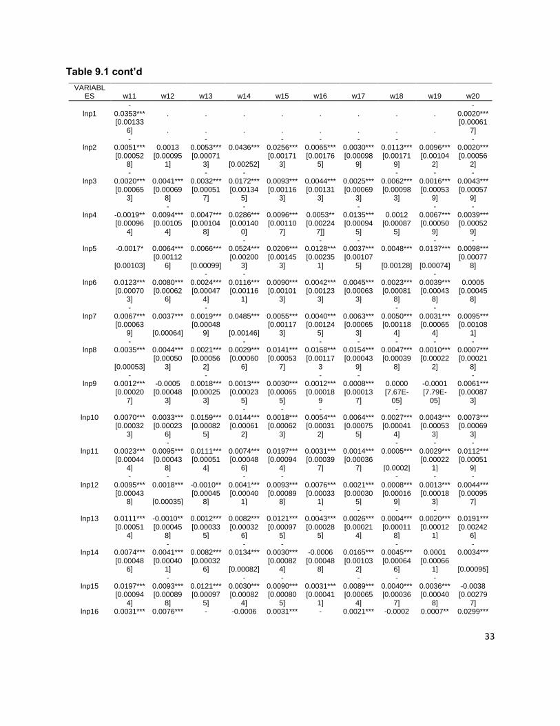
33

Table 9.1 cont’d

VARIABLES w11 w12 w13 w14 w15 w16 w17 w18 w19 w20

lnp1 -

0.0353*** . . . . . . . . -

0.0020***

[0.00133

6] . . . . . . . . [0.00061

7]

lnp2 -

0.0051*** 0.0013 -

0.0053*** 0.0436*** -

0.0256*** -

0.0065*** -

0.0030*** -

0.0113*** 0.0096*** -

0.0020***

[0.00052

8] [0.00095

1] [0.00071

3] [0.00252] [0.00171

3] [0.00176

5] [0.00098

9] [0.00171

9] [0.00104

2] [0.00056

2]

lnp3 -

0.0020*** 0.0041*** -

0.0032*** -

0.0172*** 0.0093*** 0.0044*** 0.0025*** -

0.0062*** -

0.0016*** -

0.0043***

[0.00065

3] [0.00069

8] [0.00051

7] [0.00134

5] [0.00116

3] [0.00131

3] [0.00069

3] [0.00098

3] [0.00053

9] [0.00057

9]

lnp4 -0.0019** -

0.0094*** 0.0047*** -

0.0286*** 0.0096*** 0.0053** -

0.0135*** 0.0012 -

0.0067*** -

0.0039***

[0.00096

4] [0.00105

4] [0.00104

8] [0.00140

0] [0.00110

7] [0.00224

7]] [0.00094

5] [0.00087

5] [0.00050

9] [0.00052

9]

lnp5 -0.0017* 0.0064*** 0.0066*** -

0.0524*** 0.0206*** -

0.0128*** -

0.0037*** 0.0048*** -

0.0137*** -

0.0098***

[0.00103] [0.00112

6] [0.00099] [0.00200

3] [0.00145

3] [0.00235

1] [0.00107

5] [0.00128] [0.00074] [0.00077

8]

lnp6 0.0123*** 0.0080*** -

0.0024*** -

0.0116*** 0.0090*** 0.0042*** 0.0045*** 0.0023*** -

0.0039*** 0.0005

[0.00070

3] [0.00062

6] [0.00047

4] [0.00116

1] [0.00101

3] [0.00123

3] [0.00063

3] [0.00081

8] [0.00043

8] [0.00045

8]

lnp7 -

0.0067*** 0.0037*** -

0.0019*** 0.0485*** 0.0055*** 0.0040*** 0.0063*** -

0.0050*** -

0.0031*** 0.0095***

[0.00063

9] [0.00064] [0.00048

9] [0.00146] [0.00117

3] [0.00124

5] [0.00065

3] [0.00118

4] [0.00065

4] [0.00108

1]

lnp8 -

0.0035*** 0.0044*** 0.0021*** -

0.0029*** 0.0141*** -

0.0168*** -

0.0154*** -

0.0047*** -

0.0010*** -

0.0007***

[0.00053] [0.00050

3] [0.00056

2] [0.00060

6] [0.00053

7] [0.00117

3 [0.00043

9] [0.00039

8] [0.00022

2] [0.00021

8]

lnp9 -

0.0012*** -0.0005 -

0.0018*** 0.0013*** 0.0030*** -

0.0012*** -

0.0008*** 0.0000 -0.0001 -

0.0061***

[0.00020

7] [0.00048

3] [0.00025

3] [0.00023

5] [0.00065

5] [0.00018

9 [0.00013

7] [7.67E-

05] [7.79E-

05] [0.00087

3]

lnp10 0.0070*** 0.0033*** 0.0159*** -

0.0144*** -

0.0018*** -

0.0054*** 0.0064*** -

0.0027*** 0.0043*** 0.0073***

[0.00032

3] [0.00023

6] [0.00082

5] [0.00061

2] [0.00062

3] [0.00031

2] [0.00075

5] [0.00041

4] [0.00053

3] [0.00069

3]

lnp11 0.0023*** -

0.0095*** 0.0111*** 0.0074*** 0.0197*** 0.0031*** 0.0014*** -

0.0005*** -

0.0029*** -

0.0112***

[0.00044

4] [0.00043

8] [0.00051

4] [0.00048

6] [0.00094

4] [0.00039

7] [0.00036

7] [0.0002] [0.00022

1] [0.00051

9]

lnp12 -

0.0095*** -

0.0018*** -0.0010** -

0.0041*** -

0.0093*** 0.0076*** 0.0021*** -

0.0008*** -

0.0013*** -

0.0044***

[0.00043

8] [0.00035] [0.00045

8] [0.00040

1] [0.00089

8] [0.00033

1] [0.00030

5] [0.00016

9] [0.00018

3] [0.00095

7]

lnp13 0.0111*** -0.0010** 0.0012*** 0.0082*** 0.0121*** -

0.0043*** -

0.0026*** -

0.0004*** -

0.0020*** 0.0191***

[0.00051

4] [0.00045

8] [0.00033

5] [0.00032

6] [0.00097

5] [0.00028

5] [0.00021

4] [0.00011

8] [0.00012

1] [0.00242

6]

lnp14 0.0074*** -

0.0041*** 0.0082*** -

0.0134*** -

0.0030*** -0.0006 0.0165*** -

0.0045*** 0.0001 -

0.0034***

[0.00048

6] [0.00040

1] [0.00032

6] [0.00082] [0.00082

4] [0.00048

8] [0.00103

2] [0.00064

6] [0.00066

1] [0.00095]

lnp15 0.0197*** -

0.0093*** 0.0121*** -

0.0030*** -

0.0090*** 0.0031*** -

0.0089*** -

0.0040*** -

0.0036*** -0.0038

[0.00094

4] [0.00089

8] [0.00097

5] [0.00082

4] [0.00080

5] [0.00041

1] [0.00065

4] [0.00036

7] [0.00040

8] [0.00279

7] lnp16 0.0031*** 0.0076*** - -0.0006 0.0031*** - 0.0021*** -0.0002 0.0007** 0.0299***

34

0.0043*** 0.0029***

[0.00039

7] [0.00033

1] [0.00028

5] [0.00048

8] [0.00041

1] [0.00075

2] [0.00056

5] [0.00031

2] [0.00030

8] [0.00043

5]

lnp17 0.0014*** 0.0021*** -

0.0026*** 0.0165*** -

0.0089*** 0.0021*** 0.0031*** -

0.0020*** -

0.0020*** -

0.0020***

[0.00036

7] [0.00030

5] [0.00021

4] [0.00103

2] [0.00065

4] [0.00056

5] [0.00032

2] [0.00017

8] [0.00017

8] [0.00017

8]

lnp18 -

0.0005*** -

0.0008*** -

0.0004*** -

0.0045*** -

0.0040*** -0.0002 -

0.0020*** 0.0028*** -

0.0190*** 0.0284***

[0.0002] [0.00016

9] [0.00011

8] [0.00064

6] [0.00036

7] [0.00031

2] [0.00017

8] [0.00052

7] [0.00066] [0.00042

8]

lnp19 -

0.0029*** -

0.0013*** -

0.0020*** 0.0001 -

0.0036*** 0.0007** -

0.0020*** -

0.0190*** -

0.0029*** 0.0295***

[0.00022

1] [0.00018

3] [0.00012

1] [0.00066

1] [0.00040

8] [0.00030

8] [0.00017

8] [0.00066] [0.00048

5] [0.00097

6]

lnp20 -

0.0112*** -

0.0044*** 0.0191*** -

0.0034*** -0.0038 0.0299*** -

0.0020*** 0.0284*** 0.0295*** -

0.0090***

[0.00051

9] [0.00095

7] [0.00242

6] [0.00095] [0.00279

7] [0.00043

5] [0.00017

8] [0.00042

8] [0.00097

6] [0.00071

3]

lnp21 0.0173*** 0.0014 -

0.0563*** 0.0306*** -

0.0369*** -

0.0137*** 0.0067*** 0.0218*** 0.0186*** -

0.0628***

[0.00102] [0.00139

3] [0.00287

8] [0.00319

7] [0.00353

8] [0.00308

7] [0.00209

2] [0.00206

9] [0.00155

1] [0.00471

9]

lnx 0.0001 0.0059*** -

0.0052*** 0.0176*** -

0.0049*** 0.0062*** -0.0012 -

0.0620*** 0.0137*** -

0.1256***

[0.00100

7] [0.00073

9] [0.00047] [0.00317

7] [0.00157

4] [0.00137

2] [0.00077

9] [0.00264

9] [0.00232

9] [0.00294

5]

(lnx)2 0.0008*** 0.0014*** 0.0006*** 0.0031*** 0.0002 0.0011*** 0.0002 -0.0019** 0.0047***

-0.0346***

[0.00025

4] [0.00019

7] [0.00012

8] [0.00086

5] [0.00044

1] [0.00034

3] [0.00021] [0.00075

4] [0.00059

2] [0.00082

1]

ê 0.0070*** 0.0079*** 0.0009*** 0.0006 -0.0026** 0.0072*** 0.0094*** -

0.0384*** -0.0007 -

0.0787***

[0.00052

4] [0.00048

9] [0.00032

2] [0.00060

9] [0.00115

3] [0.00066

4] [0.00052

6] [0.00186

6] [0.00118

5] [0.00260

4]

ф 0.0211*** 0.0222*** 0.0138*** 0.0392*** 0.0551*** -

0.0108*** 0.0241*** -0.079*** -

0.0317*** .

[0.00125

0] [0.00171

1] [0.00069

7] [0.00188

1] [0.00979

1] [0.00118] [0.00263

4] [0.00497

9] [0.00615] .

Constant 0.0548*** 0.0116*** 0.0551*** -0.0060 0.0651*** -

0.0287*** 0.0147*** 0.1826*** 0.0098*** 0.2393***

[0.00223

2] [0.00177

2] [0.00168

9] [0.00465

5] [0.00288

4] [0.00381

2] [0.00168

8 [0.00373

3] [0.00318

4] [0.00395

1]

Observations 21265 21265 21265 21265 21265 21265 21265 21265 21265 21265

RMSE 0.0229 0.0209 0.0135 0.035 0.0497 0.0284 0.0226 0.0842 0.0529 0.1182 R-squared 0.7068 0.6451 0.6455 0.3592 0.51 0.2534 0.5343 0.3483 0.6838 0.8188

Source: Authors‟ computation using CSA‟s HICES data. Notes: Robust standard errors in brackets. w1-w21 and lnp1-lnp20 stand for the expenditure (budget) shares and logarithm of „prices‟ respectively of teff, wheat, barley, maize, sorghum, „other cereals‟, „processed cereals‟, „pulses‟, „oil seeds‟, „animal products‟, „oil and fat‟, „vegetables and fruits‟, pepper, „enset, kocho, and bula‟, „coffee, tea, and chat‟, „root crops‟, „sugar and salt‟, „other food‟, „clothing and shoes‟, „services‟ and „other non-food‟. ***, **, and * indicate statistical significance at 1 percent, 5 percent, and 10 percent, respectively. RMSE is root mean square error. The rest of the variables and acronyms are as defined in the text.

35

Table 9.2: IFGNLS Estimates of the QU-AIDM Parameters – Rural

VARIABLES w1 w2 w3 w4 w5 w6 w7 w8 w9 w10

lnp1 0.0026 0.018*** -

0.0327*** -

0.0551*** -

0.1018*** 0.0281*** -0.0035 0.0345*** 0.0019 0.0239*** [0.01121] [0.00671] [0.00555] [0.00681] [0.0079] [0.00492] [0.00304] [0.00292] [0.00134] [0.00207]

lnp2 0.018*** 0.0087 0.0218*** -0.016*** -0.0117* 0.0148*** -0.0013 0.0086*** 0.0007 -

0.0083*** [0.00671] [0.00744] [0.00455] [0.00538] [0.00634] [0.00379] [0.00249] [0.00231] [0.00093] [0.0016]

lnp3 -

0.0327*** 0.0218*** 0.1067*** -

0.0248*** -

0.0363*** 0.003 0.0026 -

0.0145*** -0.0003 -

0.0165*** [0.00555] [0.00455] [0.00557] [0.00419] [0.00548] [0.00353] [0.00204] [0.002] [0.00072] [0.00182]

lnp4 -

0.0551*** -0.016*** -

0.0248*** 0.2998*** -

0.1179*** -0.021*** 0.0003 -

0.0111*** -

0.0056*** -

0.0215*** [0.00681] [0.00538] [0.00419] [0.00817] [0.00635] [0.00373] [0.00251] [0.00238] [0.00137] [0.00134]

lnp5 -

0.1018*** -0.0117* -

0.0363*** -

0.1179*** 0.4363*** -

0.0329*** 0.0038 0.0312*** 0.0028** -

0.0192*** [0.0079] [0.00634] [0.00548] [0.00635] [0.01002] [0.00459] [0.00289] [0.00266] [0.00124] [0.00184]

lnp6 0.0281*** 0.0148*** 0.003 -0.021*** -

0.0329*** -0.027*** 0.0033* 0.0001 0.0018*** 0.0212*** [0.00492] [0.00379] [0.00353] [0.00373] [0.00459] [0.00387] [0.00181] [0.00165] [0.00059] [0.00124]

lnp7 -0.0035 -0.0013 0.0026 0.0003 0.0038 0.0033* -0.0025 -

0.0042*** 0.0009* 0.0035*** [0.00304] [0.00249] [0.00204] [0.00251] [0.00289] [0.00181] [0.00157] [0.00107] [0.00047] [0.00069]

lnp8 0.0345*** 0.0086*** -

0.0145*** -

0.0111*** 0.0312*** 0.0001 -

0.0042*** -0.0006 0.0000 0.002*** [0.00292] [0.00231] [0.002] [0.00238] [0.00266] [0.00165] [0.00107] [0.00147] [0.00049] [0.00067]

lnp9 0.0019 0.0007 -0.0003 -

0.0056*** 0.0028** 0.0018*** 0.0009* 0.0000 0.0002 0.0011*** [0.00134] [0.00093] [0.00072] [0.00137] [0.00124] [0.00059] [0.00047] [0.00049] [0.00021] [0.00041]

lnp10 0.0239*** -

0.0083*** -

0.0165*** -

0.0215*** -

0.0192*** 0.0212*** 0.0035*** 0.002*** 0.0011*** -0.0003 [0.00207] [0.0016] [0.00182] [0.00134] [0.00184] [0.00124] [0.00069] [0.00067] [0.00041] [0.00043]

lnp11 -

0.0222*** -

0.0099*** -0.0024** -

0.0087*** 0.0048*** 0.0102*** 0.0008 -0.006*** -0.0006** 0.0072*** [0.00209] [0.00098] [0.00112] [0.00177] [0.00161] [0.00111] [0.00072] [0.00075] [0.0003] [0.00047]

lnp12 . 0.0071*** 0.0101*** 0.0014 0.0097*** 0.0026** 0.003*** 0.0035*** -

0.0024*** 0.0019*** . [0.00177] [0.00129] [0.00176] [0.00192] [0.00113] [0.00079] [0.00075] [0.00082] [0.00036]

lnp13 . -

0.0064*** -

0.0046*** 0.0075*** 0.0192*** -

0.0053*** 0.0011 0.000 -

0.0031*** 0.0432*** . [0.0015] [0.00107] [0.00203] [0.0018] [0.00093] [0.00073] [0.00084] [0.00095] [0.00135]

lnp14 . 0.0184*** -

0.0157*** 0.0028 -

0.1454*** -

0.0455*** -0.0031 -

0.0091*** 0.0011*** -

0.0123*** . [0.00491] [0.00384] [0.00467] [0.00547] [0.00361] [0.00211] [0.00192] [0.00034] [0.00093]

lnp15 . -

0.0413*** 0.0157*** 0.0056*** 0.0161*** 0.0232*** -

0.0057*** 0.0153*** 0.0021** -0.0027** . [0.0029] [0.0021] [0.00178] [0.00236] [0.00176] [0.00096] [0.0009] [0.00101] [0.00118]

lnp16 . -0.0015 -0.002 -0.0067 -

0.0393*** 0.02*** -0.005** -

0.0271*** -0.0005 -

0.0056*** . [0.00457] [0.00354] [0.00459] [0.00501] [0.00317] [0.00206] [0.00203] [0.0003] [0.00041]

lnp17 . -0.0013 -0.0007 -

0.0183*** -

0.0075*** 0.0048*** 0.0058*** -

0.0144*** -0.001*** 0.0066*** . [0.0016] [0.00119] [0.00152] [0.00173] [0.00102] [0.00069] [0.00066] [0.00023] [0.00105]

lnp18 . -0.005* -

0.0066*** 0.0025 0.008*** -0.0013 -0.0021** -

0.0081*** 0.0002 -

0.0051*** . [0.00258] [0.00183] [0.00154] [0.00212] [0.00153] [0.00084] [0.00075] [0.00013] [0.00062]

lnp19 . 0.0044*** -0.0001 -

0.0067*** -

0.0146*** -0.0014* 0.0012** -0.0007* -0.0002 0.0016* . [0.00162] [0.00103] [0.00091] [0.00128] [0.00082] [0.00048] [0.00044] [0.00014] [0.00095]

lnp20 -0.0021 -

0.0039*** -

0.0057*** -0.006*** -

0.0088*** 0.0002 0.0008 0.0009** -0.014*** 0.007*** [0.00135] [0.00124] [0.00128] [0.00109] [0.00149] [0.00096] [0.00148] [0.00045] [0.0013] [0.00084]

lnp21 0.1084*** 0.0041*** 0.0029** -0.0005 0.0035*** 0.0015 0.0003 -0.0003 0.0149*** -

36

0.0275*** [0.01018] [0.00112] [0.00131] [0.00104] [0.00127] [0.00102] [0.00024] [0.00048] [0.00138] [0.00186]

lnx 0.0036*** 0.005*** 0.0038*** 0.0044*** 0.0005 -

0.0019*** 0.002*** .*** -0.0001 0.0012 [0.00124] [0.00138] [0.00111] [0.00163] [0.00117] [0.00056] [0.00053] . [0.00015] [0.00118]

(lnx)2 0.0296*** 0.0039 -0.0001 0.0097*** 0.0041 -0.0008

-0.0077*** 0.0063*** -0.0006 0.018***

[0.00457] [0.00428] [0.00477] [0.00392] [0.00547] [0.00395] [0.00185] [0.00175] [0.00052] [0.0044] ê 0.0139*** 0.0163*** 0.0045** 0.0131*** -0.0061** 0.0019* 0.0043*** 0.0068*** 0.0006*** 0.0253*** [0.00216] [0.00273] [0.00206] [0.00247] [0.00293] [0.00106] [0.00081] [0.00135] [0.00017] [0.00233]

ф 0.0008 0.0149*** 0.0527*** 0.0156*** -

0.0506*** -

0.0101*** 0.0022 0.0243*** -0.0006* 0.0357*** [0.00351] [0.00391] [0.00369] [0.00344] [0.00393] [0.00221] [0.00161] [0.00336] [0.00037] [0.00443]

Constant 0.2074*** 0.052*** 0.0954*** 0.1856*** 0.0466*** -

0.0561*** 0.0215*** 0.0249*** 0.0015 0.0857*** [0.0162] [0.01146] [0.00933] [0.00944] [0.01083] [0.00735] [0.00408] [0.00399] [0.00179] [0.00619]

Observations 9440 9440 9440 9440 9440 9440 9440 9440 9440 9440

RMSE 0.061 0.0731 0.0569 0.0636 0.0808 0.0303 0.0242 0.0358 0.0048 0.0622 R-squared 0.3997 0.4388 0.2489 0.4876 0.4896 0.2124 0.2015 0.6126 0.1228 0.4583

Source: Authors‟ computation using CSA‟s HICES data. Notes: Robust standard errors in brackets. w1-w21 and lnp1-lnp20 stand for the expenditure (budget) shares and logarithm of „prices‟ respectively of teff, wheat, barley, maize, sorghum, „other cereals‟, „processed cereals‟, „pulses‟, „oil seeds‟, „animal products‟, „oil and fat‟, „vegetables and fruits‟, pepper, „enset, kocho, and bula‟, „coffee, tea, and chat‟, „root crops‟, „sugar and salt‟, „other food‟, „clothing and shoes‟, „services‟ and „other non-food‟. ***, **, and * indicate statistical significance at 1 percent, 5 percent, and 10 percent, respectively. RMSE is root mean square error. The rest of the variables and acronyms are as defined in the text.

37

Table 9.2 cont’d

VARIABLES w11 w12 w13 w14 w15 w16 w17 w18 w19 w20

lnp1 -

0.0222*** . . . . . . . . -0.0021 [0.00209] . . . . . . . . [0.00135]

lnp2 -

0.0099*** 0.0071*** -

0.0064*** 0.0184*** -

0.0413*** -0.0015 -0.0013 -0.005* 0.0044*** -

0.0039*** [0.00098] [0.00177] [0.0015] [0.00491] [0.0029] [0.00457] [0.0016] [0.00258] [0.00162] [0.00124]

lnp3 -0.0024** 0.0101*** -

0.0046*** -

0.0157*** 0.0157*** -0.002 -0.0007 -

0.0066*** -0.0001 -

0.0057*** [0.00112] [0.00129] [0.00107] [0.00384] [0.0021] [0.00354] [0.00119] [0.00183] [0.00103] [0.00128]

lnp4 -

0.0087*** 0.0014 0.0075*** 0.0028 0.0056*** -0.0067 -

0.0183*** 0.0025 -

0.0067*** -0.006*** [0.00177] [0.00176] [0.00203] [0.00467] [0.00178] [0.00459] [0.00152] [0.00154] [0.00091] [0.00109]

lnp5 0.0048*** 0.0097*** 0.0192*** -

0.1454*** 0.0161*** -

0.0393*** -

0.0075*** 0.008*** -

0.0146*** -

0.0088*** [0.00161] [0.00192] [0.0018] [0.00547] [0.00236] [0.00501] [0.00173] [0.00212] [0.00128] [0.00149]

lnp6 0.0102*** 0.0026** -

0.0053*** -

0.0455*** 0.0232*** 0.02*** 0.0048*** -0.0013 -0.0014* 0.0002 [0.00111] [0.00113] [0.00093] [0.00361] [0.00176] [0.00317] [0.00102] [0.00153] [0.00082] [0.00096]

lnp7 0.0008 0.003*** 0.0011 -0.0031 -

0.0057*** -0.005** 0.0058*** -0.0021** 0.0012** 0.0008 [0.00072] [0.00079] [0.00073] [0.00211] [0.00096] [0.00206] [0.00069] [0.00084] [0.00048] [0.00148]

lnp8 -0.006*** 0.0035*** 0.0000 -

0.0091*** 0.0153*** -

0.0271*** -

0.0144*** -

0.0081*** -0.0007 0.0009* [0.00075] [0.00075] [0.00084] [0.00192] [0.0009] [0.00203] [0.00066] [0.00075] [0.00044] [0.00045]

lnp9 -0.0006** -

0.0024*** -

0.0031*** 0.0011*** 0.0021** -0.0005 -0.001*** 0.0002 -0.0002 -0.014*** [0.0003] [0.00082] [0.00095] [0.00034] [0.00101] [0.0003] [0.00023] [0.00013] [0.00014] [0.0013]

lnp10 0.0072*** 0.0019*** 0.0432*** -

0.0123*** -0.0027** -

0.0056*** 0.0066*** -

0.0051*** 0.0016 0.007*** [0.00047] [0.00036] [0.00135] [0.00093] [0.00118] [0.00041] [0.00105] [0.00062] [0.00095] [0.00084]

lnp11 0.0044*** -

0.0088*** 0.006*** 0.0029*** 0.0226*** 0.0013*** 0.0006 -

0.0011*** -

0.0038*** -

0.0124*** [0.00057] [0.00064] [0.00143] [0.00063] [0.00152] [0.0005] [0.00052] [0.00029] [0.00036] [0.00071]

lnp12 -

0.0088*** -0.0005 -

0.0193*** -

0.0073*** 0.0004 0.004*** 0.0013** -0.0001 -

0.0031*** -

0.0132*** [0.00064] [0.0005] [0.0015] [0.0006] [0.0015] [0.00046] [0.00051] [0.0003] [0.00036] [0.00165]

lnp13 0.006*** -

0.0193*** 0.0042*** 0.0079*** 0.0097*** -

0.0037*** -

0.0039*** -

0.0006*** -

0.0025*** 0.1656*** [0.00143] [0.0015] [0.00134] [0.00056] [0.00158] [0.00045] [0.00039] [0.00022] [0.00025] [0.00645]

lnp14 0.0029*** -

0.0073*** 0.0079*** -

0.0057*** 0.0228*** 0.0015 0.0178*** -0.0003 -

0.0067*** 0.012*** [0.00063] [0.0006] [0.00056] [0.00173] [0.00374] [0.00137] [0.00171] [0.00103] [0.00108] [0.00148]

lnp15 0.0226*** 0.0004 0.0097*** 0.0228*** -

0.0167*** 0.004*** -

0.0088*** -0.0015** -

0.0027*** 0.0021 [0.00152] [0.0015] [0.00158] [0.00374] [0.00161] [0.00055] [0.00102] [0.00062] [0.00084] [0.00519]

lnp16 0.0013*** 0.004*** -

0.0037*** 0.0015 0.004*** 0.006*** 0.0052*** 0.0015* 0.0003 0.0266*** [0.0005] [0.00046] [0.00045] [0.00137] [0.00055] [0.00132] [0.00136] [0.00082] [0.0009] [0.00059]

lnp17 0.0006 0.0013** -

0.0039*** 0.0178*** -

0.0088*** 0.0052*** 0.0009** -

0.0012*** -

0.0031*** -0.0017 [0.00052] [0.00051] [0.00039] [0.00171] [0.00102] [0.00136] [0.00047] [0.00027] [0.00033] [0.00147]

lnp18 -

0.0011*** -0.0001 -

0.0006*** -0.0003 -0.0015** 0.0015* -

0.0012*** 0.0018*** -

0.0179*** 0.0244*** [0.00029] [0.0003] [0.00022] [0.00103] [0.00062] [0.00082] [0.00027] [0.00067] [0.00091] [0.0006]

lnp19 -

0.0038*** -

0.0031*** -

0.0025*** -

0.0067*** -

0.0027*** 0.0003 -

0.0031*** -

0.0179*** -

0.0042*** 0.0396*** [0.00036] [0.00036] [0.00025] [0.00108] [0.00084] [0.0009] [0.00033] [0.00091] [0.0007] [0.00131]

lnp20 -

0.0124*** -

0.0132*** 0.1656*** 0.012*** 0.0021 0.0266*** -0.0017 0.0244*** 0.0396*** -0.005*** [0.00071] [0.00165] [0.00645] [0.00148] [0.00519] [0.00059] [0.00147] [0.0006] [0.00131] [0.00136]

lnp21 0.0151*** 0.0098*** -0.215*** 0.1641*** - 0.0212*** 0.0188*** 0.0126*** 0.0207*** -

38

0.0601*** 0.2064*** [0.00135] [0.00233] [0.00733] [0.00748] [0.00692] [0.00639] [0.00334] [0.0032] [0.00258] [0.00945]

lnx -0.0002 0.0009** 0.0006** -0.0014 -

0.0022*** 0.0036*** 0.0004 -

0.0046*** 0.0000 -

0.0131*** [0.00038] [0.00036] [0.00024] [0.00136] [0.00085] [0.00098] [0.00033] [0.00098] [0.00081] [0.00113]

(lnx)2

-0.0043*** 0.005***

-0.0062*** 0.0191*** 0.0071** 0.0094***

-0.0044***

-0.0616*** 0.0119***

-0.1244***

[0.00151] [0.00126] [0.00085] [0.00444] [0.0029] [0.00363] [0.00112] [0.00332] [0.00323] [0.00385]

ê 0.0004 0.0035*** -0.0007 -0.0006 0.0053** 0.0099*** 0.0032*** -

0.0235*** 0.0016 -

0.0641*** [0.00075] [0.00095] [0.0006] [0.00146] [0.00236] [0.0015] [0.00089] [0.00254] [0.00179] [0.00348]

ф 0.0209*** 0.0079*** 0.0185*** 0.0089*** 0.0367*** -

0.0137*** 0.0303*** 0.0025 -0.0091 .*** [0.00144] [0.00254] [0.00099] [0.00315] [0.01228] [0.00232] [0.00788] [0.00567] [0.00814] .

Constant 0.0603*** 0.0117*** 0.0779*** 0.1024*** 0.0376*** -0.0039 0.0314*** 0.1954*** 0.0173*** 0.2188*** [0.00344] [0.00296] [0.00308] [0.00875] [0.00523] [0.00834] [0.0026] [0.00524] [0.00466] [0.00541]

Observations 9440 9440 9440 9440 9440 9440 9440 9440 9440 9440

RMSE 0.0194 0.0243 0.0153 0.0466 0.0599 0.0403 0.0224 0.0664 0.0472 0.0891 R-squared 0.5049 0.519 0.5756 0.48 0.5496 0.244 0.4577 0.4435 0.6983 0.8609

Source: Authors‟ computation using CSA‟s HICES data. Notes: Robust standard errors in brackets. w1-w21 and lnp1-lnp20 stand for the expenditure (budget) shares and logarithm of „prices‟ respectively of teff, wheat, barley, maize, sorghum, „other cereals‟, „processed cereals‟, „pulses‟, „oil seeds‟, „animal products‟, „oil and fat‟, „vegetables and fruits‟, pepper, „enset, kocho, and bula‟, „coffee, tea, and chat‟, „root crops‟, „sugar and salt‟, „other food‟, „clothing and shoes‟, „services‟ and „other non-food‟. ***, **, and * indicate statistical significance at 1 percent, 5 percent, and 10 percent, respectively. RMSE is root mean square error. The rest of the variables and acronyms are as defined in the text.

39

Table 9.3: IFGNLS Estimates of the QU-AIDM Parameters – Urban

VARIABLES w1 w2 w3 w4 w5 w6 w7 w8 w9 w10

lnp1 0.0472*** 0.003 -

0.0074*** -

0.0102*** -

0.0765*** 0.0132*** -

0.0152*** 0.0039** 0.0046*** 0.0146*** [0.00634] [0.00282] [0.00202] [0.00305] [0.00393] [0.00235] [0.00359] [0.00169] [0.00091] [0.00183]

lnp2 0.003 -0.0027 0.0046*** 0.0068*** -0.002 -

0.0092*** 0.0124*** 0.0007 -0.0006 -

0.0129*** [0.00282] [0.00249] [0.00123] [0.00193] [0.00234] [0.00139] [0.00193] [0.00100] [0.00048] [0.00102]

lnp3 -

0.0074*** 0.0046*** 0.0201*** -0.0013 -

0.0094*** -0.006*** 0.0065*** -

0.0049*** -0.0004 -

0.0056*** [0.00202] [0.00123] [0.00128] [0.00132] [0.00156] [0.00094] [0.00131] [0.00074] [0.00039] [0.00071]

lnp4 -

0.0102*** 0.0068*** -0.0013 0.0886*** -

0.0401*** 0.0046*** 0.0102*** -

0.0087*** -

0.0029*** -

0.0089*** [0.00305] [0.00193] [0.00132] [0.00316] [0.00260] [0.00129] [0.00162] [0.00123] [0.00077] [0.00089]

lnp5 -

0.0765*** -0.002 -

0.0094*** -

0.0401*** 0.106*** -

0.0135*** 0.0011 0.0188*** 0.0016** -

0.0081*** [0.00393] [0.00234] [0.00156] [0.00260] [0.00396] [0.00169] [0.00231] [0.00135] [0.00076] [0.00118]

lnp6 0.0132*** -

0.0092*** -0.006*** 0.0046*** -

0.0135*** -0.0018 -0.011*** -

0.0043*** 0.0002 0.0007 [0.00235] [0.00139] [0.00094] [0.00129] [0.00169] [0.00147] [0.00187] [0.00074] [0.00032] [0.00092]

lnp7 -

0.0152*** 0.0124*** 0.0065*** 0.0102*** 0.0011 -0.011*** -

0.0439*** 0.0013 0.0017*** -0.0005 [0.00359] [0.00193] [0.00131] [0.00162] [0.00231] [0.00187] [0.00496] [0.00099] [0.00042] [0.00179]

lnp8 0.0039** 0.0007 -

0.0049*** -

0.0087*** 0.0188*** -

0.0043*** 0.0013 0.0002 0.0004 0.0029*** [0.00169] [0.00100] [0.00074] [0.00123] [0.00135] [0.00074] [0.00099] [0.00112] [0.00056] [0.00054]

lnp9 0.0046*** -0.0006 -0.0004 -

0.0029*** 0.0016** 0.0002 0.0017*** 0.0004 0.0007*** -

0.0011*** [0.00091] [0.00048] [0.00039] [0.00077] [0.00076] [0.00032] [0.00042] [0.00056] [0.00024] [0.00039]

lnp10 0.0146*** -

0.0129*** -

0.0056*** -

0.0089*** -

0.0081*** 0.0007 -0.0005 0.0029*** -

0.0011*** 0.0027*** [0.00183] [0.00102] [0.00071] [0.00089] [0.00118] [0.00092] [0.00179] [0.00054] [0.00039] [0.00064]

lnp11 -0.027*** -0.0001 -0.0014** -

0.0037*** 0.0005 0.0059*** -

0.0043*** -

0.0059*** -

0.0027*** 0.0049*** [0.00179] [0.00057] [0.00068] [0.00099] [0.00119] [0.00079] [0.00096] [0.00069] [0.00037] [0.00046]

lnp12 . 0.0016* -0.0007 -

0.0162*** 0.0117*** 0.0079*** 0.0057*** 0.0033*** -0.0005 0.0029*** . [0.00096] [0.00064] [0.00104] [0.00117] [0.00066] [0.00085] [0.00066] [0.00056] [0.00035]

lnp13 . -

0.0031*** -0.003*** 0.0025** -0.0008 -0.001** -0.0011* 0.0067*** -0.0002 0.0064*** . [0.00071] [0.00050] [0.00105] [0.00106] [0.00051] [0.00064] [0.00074] [0.00023] [0.00071]

lnp14 . 0.0042** 0.0005 -

0.0115*** -0.0008 0.001 0.0293*** 0.0018*** 0.0013*** -

0.0053*** . [0.00176] [0.00063] [0.00086] [0.00115] [0.00091] [0.00141] [0.00049] [0.00029] [0.00082]

lnp15 . -0.0036** 0.0031*** 0.0082*** 0.0117*** 0.0055*** -0.0016 0.0103*** 0.0009 -

0.0012*** . [0.00177] [0.00080] [0.00110] [0.00139] [0.00103] [0.00154] [0.00061] [0.00069] [0.00042]

lnp16 . 0.0017** 0.0015** 0.0029** 0.0058*** 0.0034*** 0.0027*** -

0.0084*** -

0.0006*** -

0.0087*** . [0.00087] [0.00062] [0.00131] [0.00138] [0.00064] [0.00076] [0.00093] [0.00023] [0.00056]

lnp17 . -

0.0038*** 0.0063*** -

0.0136*** 0.0006 0.0051*** -

0.0039*** -0.013*** -

0.0006*** 0.0038*** . [0.00120] [0.00068] [0.00093] [0.00111] [0.00082] [0.00105] [0.00057] [0.00013] [0.00089]

lnp18 . 0.0001 -

0.0014*** -0.0008 -0.0002 0.0041*** -0.005*** -

0.0035*** -0.0001* 0.0005 . [0.00195] [0.00051] [0.00065] [0.00089] [0.00076] [0.00168] [0.00036] [0.00009] [0.00049]

lnp19 . 0.0032*** -

0.0011*** -

0.0047*** -

0.0059*** -

0.0055*** -

0.0095*** -

0.0009*** -0.0002** 0.0023*** . [0.00113] [0.00027] [0.00037] [0.00052] [0.00042] [0.00091] [0.00020] [0.00006] [0.00046]

lnp20 -

0.0083*** -

0.0045*** -

0.0017*** -

0.0035*** -

0.0052*** -

0.0015*** 0.0272*** -

0.0016*** 0.0131*** 0.0229*** [0.00058] [0.00036] [0.00024] [0.00030] [0.00044] [0.00035] [0.00138] [0.00017] [0.00126] [0.00115]

40

lnp21 0.0582*** 0.004*** 0.0016*** 0.0024*** 0.0049*** 0.0023*** -

0.0021*** 0.0007*** -

0.0144*** -

0.0124*** [0.00538] [0.00042] [0.00027] [0.00036] [0.00051] [0.00041] [0.00042] [0.00019] [0.00127] [0.00184]

Lnx -

0.0024*** -0.0005 -0.0008 -0.0018** -0.0008 0.0075*** 0.001*** . -

0.0003*** 0.0029*** [0.00055] [0.00035] [0.00052] [0.00073] [0.00054] [0.00126] [0.00026] . [0.00011] [0.00070]

(lnx)2 0.003

-0.0171***

-0.0066***

-0.0114***

-0.0221***

-0.0081*** 0.0062***

-0.0041***

-0.0008*** 0.0226***

[0.00180] [0.00116] [0.00080] [0.00093] [0.00123] [0.00113] [0.00208] [0.00051] [0.00018] [0.00147]

ê 0.0336*** 0.0092*** 0.0016*** -0.0006 -

0.0039*** 0.0016*** 0.0227*** 0.0109*** 0.0001 0.0217*** [0.00166] [0.00092] [0.00039] [0.00053] [0.00065] [0.00049] [0.00233] [0.00054] [0.00004] [0.00125]

ф -0.015*** 0.0379*** 0.01*** 0.0182*** 0.0252*** 0.0063*** 0.0215*** -0.0028 0.0007*** 0.0431*** [0.00308] [0.00207] [0.00126] [0.00116] [0.00167] [0.00118] [0.00720] [0.00179] [0.00023] [0.00431]

Constant 0.2166*** 0.0462*** 0.0298*** 0.0804*** 0.0917*** 0.028*** 0.2009*** 0.0343*** 0.0031*** 0.0277*** [0.00745] [0.00415] [0.00269] [0.00342] [0.00415] [0.00289] [0.00474] [0.00198] [0.00106] [0.00298]

Observations 11825 11825 11825 11825 11825 11825 11825 11825 11825 11825

RMSE 0.0611 0.0325 0.014 0.0195 0.0239 0.0191 0.0961 0.0188 0.0018 0.0454 R-squared 0.6946 0.408 0.1101 0.4052 0.2731 0.2205 0.422 0.7458 0.0765 0.6192

Source: Authors‟ computation using CSA‟s HICES data. Notes: Robust standard errors in brackets. w1-w21 and lnp1-lnp20 stand for the expenditure (budget) shares and logarithm of „prices‟ respectively of teff, wheat, barley, maize, sorghum, „other cereals‟, „processed cereals‟, „pulses‟, „oil seeds‟, „animal products‟, „oil and fat‟, „vegetables and fruits‟, pepper, „enset, kocho, and bula‟, „coffee, tea, and chat‟, „root crops‟, „sugar and salt‟, „other food‟, „clothing and shoes‟, „services‟ and „other non-food‟. ***, **, and * indicate statistical significance at 1 percent, 5 percent, and 10 percent, respectively. RMSE is root mean square error. The rest of the variables and acronyms are as defined in the text.

41

Table 9.3 cont’d

VARIABLES w11 w12 w13 w14 w15 w16 w17 w18 w19 w20

lnp1 -0.027*** . . . . . . . . -

0.0083*** [0.00179] . . . . . . . . [0.00058]

lnp2 -0.0001 0.0016* -

0.0031*** 0.0042** -0.0036** 0.0017** -

0.0038*** 0.0001 0.0032*** -

0.0045*** [0.00057] [0.00096] [0.00071] [0.00176] [0.00177] [0.00087] [0.00120] [0.00195] [0.00113] [0.00036]

lnp3 -0.0014** -0.0007 -0.003*** 0.0005 0.0031*** 0.0015*** 0.0063*** -

0.0014*** -

0.0011*** -

0.0017*** [0.00068] [0.00064] [0.00050] [0.00063] [0.00080] [0.00062] [0.00068] [0.00051] [0.00027] [0.00024]

lnp4 -

0.0037*** -

0.0162*** 0.0025** -

0.0115*** 0.0082*** 0.0029** -

0.0136*** -0.0008 -

0.0047*** -

0.0035*** [0.00099] [0.00104] [0.00105] [0.00086] [0.00110] [0.00131] [0.00093] [0.00065] [0.00037] [0.00030]

lnp5 0.0005 0.0117*** -0.0008 -0.0008 0.0117*** 0.0058*** 0.0006 -0.0002 -

0.0059*** -

0.0052*** [0.00119] [0.00117] [0.00106] [0.00115] [0.00139] [0.00138] [0.00111] [0.00089] [0.00052] [0.00044]

lnp6 0.0059*** 0.0079*** -0.001** 0.001 0.0055*** 0.0034*** 0.0051*** 0.0041*** -

0.0055*** -

0.0015*** [0.00079] [0.00066] [0.00051] [0.00091] [0.00103] [0.00064] [0.00082] [0.00076] [0.00042] [0.00035]

lnp7 -

0.0043*** 0.0057*** -0.0011* 0.0293*** -0.0016 0.0027*** -

0.0039*** -0.005*** -

0.0095*** 0.0272*** [0.00096] [0.00085] [0.00064] [0.00141] [0.00154] [0.00076] [0.00105] [0.00168] [0.00091] [0.00138]

lnp8 -

0.0059*** 0.0033*** 0.0067*** 0.0018*** 0.0103*** -

0.0084*** -0.013*** -

0.0035*** -

0.0009*** -

0.0016*** [0.00069] [0.00066] [0.00074] [0.00049] [0.00061] [0.00093] [0.00057] [0.00036] [0.00020] [0.00017]

lnp9 -

0.0027*** -0.0005 -0.0002 0.0013*** 0.0009 -

0.0006*** -

0.0006*** -0.0001* -0.0002** 0.0131*** [0.00037] [0.00056] [0.00023] [0.00029] [0.00069] [0.00023] [0.00013] [0.00009] [0.00006] [0.00126]

lnp10 0.0049*** 0.0029*** 0.0064*** -

0.0053*** -

0.0012*** -

0.0087*** 0.0038*** 0.0005 0.0023*** 0.0229*** [0.00046] [0.00035] [0.00071] [0.00082] [0.00042] [0.00056] [0.00089] [0.00049] [0.00046] [0.00115]

lnp11 0.001 -

0.0117*** 0.0062*** 0.0088*** 0.0062*** 0.0022*** 0.0016*** 0.0000 -

0.0014*** -

0.0094*** [0.00066] [0.00064] [0.00058] [0.00074] [0.00076] [0.00064] [0.00046] [0.00025] [0.00023] [0.00075]

lnp12 -

0.0117*** -0.002*** -0.004*** 0.0003 -

0.0074*** 0.0084*** 0.001*** -

0.0014*** -

0.0008*** 0.0017*** [0.00064] [0.00051] [0.00044] [0.00054] [0.00067] [0.00049] [0.00033] [0.00018] [0.00016] [0.00114]

lnp13 0.0062*** -0.004*** 0.0028*** 0.0064*** 0.0086*** -

0.0052*** -

0.0017*** 0.0001 -

0.0012*** -

0.0093*** [0.00058] [0.00044] [0.00033] [0.00041] [0.00101] [0.00040] [0.00023] [0.00013] [0.00011] [0.00105]

lnp14 0.0088*** 0.0003 0.0064*** -

0.0066*** -

0.0043*** -

0.0053*** 0.0005 -

0.0013*** -

0.0033*** -

0.0301*** [0.00074] [0.00054] [0.00041] [0.00073] [0.00039] [0.00051] [0.00067] [0.00042] [0.00026] [0.00111]

lnp15 0.0062*** -

0.0074*** 0.0086*** -

0.0043*** -0.002*** 0.0061*** -

0.0053*** -

0.0045*** -

0.0051*** -

0.0094*** [0.00076] [0.00067] [0.00101] [0.00039] [0.00050] [0.00063] [0.00069] [0.00038] [0.00034] [0.00181]

lnp16 0.0022*** 0.0084*** -

0.0052*** -

0.0053*** 0.0061*** -0.005*** -0.0002 -

0.0012*** -

0.0013*** 0.0355*** [0.00064] [0.00049] [0.00040] [0.00051] [0.00063] [0.0005] [0.0003] [0.0002] [0.0001] [0.0007]

lnp17 0.0016*** 0.001*** -

0.0017*** 0.0005 -

0.0053*** -0.0002 0.0044*** -

0.0029*** -

0.0007*** 0.0083*** [0.00046] [0.00033] [0.00023] [0.00067] [0.00069] [0.0003] [0.00042] [0.00023] [0.00020] [0.00185]

lnp18 0.0000 -

0.0014*** 0.0001 -

0.0013*** -

0.0045*** -

0.0012*** -

0.0029*** 0.0021*** -

0.0178*** 0.0304*** [0.00025] [0.00018] [0.00013] [0.00042] [0.00038] [0.0002] [0.00023] [0.00075] [0.00082] [0.00060]

lnp19 -

0.0014*** -

0.0008*** -

0.0012*** -

0.0033*** -

0.0051*** -

0.0013*** -

0.0007*** -

0.0178*** -

0.0067*** 0.0422*** [0.00023] [0.00016] [0.00011] [0.00026] [0.00034] [0.0001] [0.00020] [0.00082] [0.00050] [0.00108]

lnp20 -

0.0094*** 0.0017 -

0.0093*** -

0.0301*** -

0.0094*** 0.0355*** 0.0083*** 0.0304*** 0.0422*** -

0.0089*** [0.00075] [0.00114] [0.00105] [0.00111] [0.00181] [0.0007] [0.00185] [0.00060] [0.00108] [0.00095]

42

lnp21 0.0305*** 0.0002 -

0.0093*** 0.0144*** -

0.0161*** -

0.0344*** 0.0142*** 0.0029 0.0185*** -0.088*** [0.00158] [0.00174] [0.00200] [0.00245] [0.00283] [0.0023] [0.00259] [0.00250] [0.00162] [0.00441]

lnx 0.0024*** 0.0023*** 0.0005*** 0.0006 -

0.0014*** 0.0002 0.0011*** -0.0005 0.0043*** -

0.0329*** [0.00036] [0.00024] [0.00017] [0.00048] [0.00049] [0.00021] [0.00030] [0.00125] [0.00084] [0.00159]

(lnx)2 0.0047*** 0.0047***

-0.0038*** -0.0015*

-0.0109***

-0.0031*** 0.0035***

-0.0574***

-0.0092***

-0.0287***

[0.00073] [0.00047] [0.00035] [0.00089] [0.00091] [0.00049] [0.00057] [0.00219] [0.00157] [0.00274]

ê 0.0131*** 0.0099*** 0.0035*** 0.0000 -

0.0039*** 0.002*** 0.0107*** -

0.0419*** -

0.0041*** -

0.0874*** [0.00068] [0.00049] [0.00034] [0.00018] [0.00106] [0.00036] [0.00063] [0.00260] [0.00163] [0.00345]

ф -0.005** 0.0022 0.0003 0.0226*** -0.0021 0.0097*** -

0.0066*** -

0.0688*** 0.0069 . [0.00237] [0.00197] [0.00115] [0.00093] [0.01207] [0.00100] [0.00249] [0.01052] [0.00948] .

Constant 0.0222*** 0.0133*** 0.0344*** 0.0115*** 0.0875*** 0.0053** 0.0121*** 0.1157*** 0.0328*** 0.1642*** [0.00236] [0.00170] [0.00178] [0.00235] [0.00246] [0.00238] [0.00180] [0.00352] [0.00237] [0.00333]

Observations 11825 11825 11825 11825 11825 11825 11825 11825 11825 11825

RMSE 0.0239 0.017 0.0118 0.0081 0.037 0.012 0.0222 0.0953 0.0563 0.128 R-squared 0.7806 0.7668 0.7155 0.361 0.4941 0.3875 0.6006 0.3146 0.6844 0.824

Source: Authors‟ computation using CSA‟s HICES data. Notes: Robust standard errors in brackets. w1-w21 and lnp1-lnp20 stand for the expenditure (budget) shares and logarithm of „prices‟ respectively of teff, wheat, barley, maize, sorghum, „other cereals‟, „processed cereals‟, „pulses‟, „oil seeds‟, „animal products‟, „oil and fat‟, „vegetables and fruits‟, pepper, „enset, kocho, and bula‟, „coffee, tea, and chat‟, „root crops‟, „sugar and salt‟, „other food‟, „clothing and shoes‟, „services‟ and „other non-food‟. ***, **, and * indicate statistical significance at 1 percent, 5 percent, and 10 percent, respectively. RMSE is root mean square error. The rest of the variables and acronyms are as defined in the text.

43

Table 10 – Households with zero expenditure, by commodity group

Commodity Group

Households with zero

expenditure (%)

Teff 33.7

Wheat 22.5

Barley 50.3

Maize 37.3

Sorghum 47.6

Other Cereals 64.3

Processed Cereals 21.1

Pulses 4.7

Oil-Seeds 75.1

Animal-Products 11.1

Oils and Fats 11.6

Fruits and Vegetables 3.6

Pepper 10.4

Enset/Kocho/Bulla 82.6

Coffee/Tea/Chat 0.6

Root Crops 27.1

Sugar and Salt 1.6

Other Food 4.9

Clothing and Shoes 3.2

Services 0.0

Other Non-food 0.1

Total 24.4 Source: Authors‟ computation using HICES data. Notes: The figures in the second column are the fraction of the sample households who reported no expenditure on the respective commodity group during the survey period.

44

Table 11: Commodity Groups

Other Cereals Processed Cereal

Pulses Oilseeds Animal Products

Oils and Fats Finger millet Spaghetti Horse beans Niger seed Beef Butter

Rice Past Chick peas Linseed Mutton Edible oil

Oats/'Aja' Maccaroni Peas Sesame Chicken Ground nuts butter Others Injera Lentils Sunflower Pork Bread Haricot beans Castor beans Canned meat Cakes Vetch Ground nuts Goat meat Porridge Fenugreek Others Birds Others Soya-bean

Wild animals

Others

Offal

Fish

Milk

Yoghurt

Eggs

Honey

Others

Fruits and Vegetables Pepper Enset/ kocho/bulla Coffee/ tea/chat

Root crops Sugar and salt Ethiopian kale Pepper whole Kocho Coffee Potato Sugar

Cabbage Pepper flour Bulla Tea Sweet potato Salt

Lettuce Pepper sauce Kocho pancake Chat Anchote Spinach

Others Cassava

Carrot

Others Tomato

Onions

Garlic

Banana

Orange

Avocado

Others

Other foods Clothing Services Other

and shoes

non-foods

Spices like: Clothing Milling charges Cigarettes Corriander Shoes Rent Construction

materials like: Cinnamon

Transportation costs Bricks Cloves etc.

Salary for servants Water pipe

Processed foods like:

Medical expenses Corrugated iron sheets Lazanga

Schooling related expenses like:

Door set Burger/sandwich

Registration fee Paints etc

Halawa

Tution fee etc. Furniture like: 'Key wot'

Others Tables

'Tibs'

Chairs 'Minchitabish' etc.

Sofas

Beverages like:

Coca cola family

Pepsi family

Mineral water etc.

Juices

Alcholic drinks like:

Cognac

Brandy

Gin

Katikala etc.

Others

45

APPENDIX II: DERIVATION OF ELASTICITY OF DEMAND FOR QU-AIDM

Recall that the ith budget share equation for the QU-AIDM is given by:

2

1

ln ln ln( ) ( ) ( )

ni

i i ij j ij

x xw p

a b ap p p

where:

0

1 1 1

1

1ln ( ) ln ln ln

2

( ) k

n n n

k k kj k jk k j

n

kk

a p p p

b p

p

p

and p and x stand for prices and total expenditure, respectively.

Price elasticities

Since i ii

p qw

m, the uncompensated own-price and the cross-price elasticities respectively

are:

2

,1

,1

21ln (ln ln ( )) ln ln ( ) 1

( ) ( )

21ln (ln ln ( ))

( ) (

i

j

ni i

i p ii i kj k i iki

nji i

i p ij j kj k iki j

p x a x aw b b

pp x a

w p b b

p pp p

pp p

2ln ln ( )

) ix a p

Corresponding compensated price elasticities are:

, , ,

, , ,

i i

j j

i p i p i x i

i p i p i x j

w

w

Expenditure elasticities Similarly, the expenditure elasticity of demand for commodity i (qi) is given by:

,

1 2ln ln ( ) 1

( )i i

i x ii i

x qx a

q x w bp

p

46

A note on unit values

Since i ii

u qw

x , where ui is the unit value of commodity i, we have:

ii

i

w xq

u

such that:

2

( ) 1

ln ln

i ii i i i i

i i i

w x uq w w u w

x x x u u x u

Then:

,

1 11

ln lni i i

i xi i i

x q w u

q x w x u x

Since ln ln 1

ln ln ln

z z z z

y z y z y :

,

, ,

ln ln1

ln ln1

i

i i

i iq x

s x u x

w u

x x

Thus, according to the approach developed by Deaton, the use of unit values necessitates the

adjustment of expenditure elasticity of quantity demanded to account for the „quality‟ elasticity of

the commodity‟s unit value.

47

Table 12: Estimated Quality (or expenditure) Elasticity of Unit Values

Commodity Coefficient Standard

Error t P-value

95% Confidence Interval

Teff 0.035 0.004 9.850 0.000 0.028 0.042

Wheat 0.035 0.004 8.580 0.000 0.027 0.043

Barley -0.002 0.007 -0.330 0.742 -0.017 0.012

Maize -0.006 0.004 -1.590 0.112 -0.013 0.001

Sorghum -0.018 0.004 -4.370 0.000 -0.026 -0.010

Other Cereals 0.036 0.010 3.630 0.000 0.016 0.055

Processed Cereals 0.088 0.007 13.460 0.000 0.075 0.101

Pulses 0.053 0.004 12.370 0.000 0.045 0.062

Oil-Seeds -0.009 0.007 -1.260 0.210 -0.024 0.005

Animal-Products 0.095 0.010 9.190 0.000 0.075 0.115

Oils and Fats 0.067 0.005 13.080 0.000 0.057 0.076

Fruits and Vegetables 0.148 0.007 19.930 0.000 0.133 0.162

Pepper 0.006 0.003 1.900 0.058 0.000 0.011

Enset/Kocho/Bulla 0.106 0.017 6.150 0.000 0.072 0.140

Coffee/Tea/Chat 0.026 0.006 4.170 0.000 0.014 0.038

Root Crops 0.040 0.005 8.780 0.000 0.031 0.049

Sugar and Salt 0.172 0.008 22.560 0.000 0.157 0.187

Other Food 0.093 0.010 9.530 0.000 0.074 0.113

Clothing and Shoes 0.518 0.017 30.000 0.000 0.484 0.552

Services 1.181 0.022 53.580 0.000 1.138 1.225

Other Non-food 1.939 0.040 48.990 0.000 1.861 2.017

Source: Authors‟ computation using HICES data and the estimation procedure in Deaton (1997).