focusing on imaging high performance vereos pet/ct

Vereos PET/CT

Advanced Molecular Imaging

Focusing on high performance

Michael A. Miller, PhD, Philips, Advanced Molecular Imaging Physics

This white paper presents a description of the Vereos digital PET/CT system and the results of PET performance measurements made on the Vereos digital PET/CT research system installed at The Ohio State University in Columbus, Ohio, USA, and on several pre-production systems built and tested at Philips Advanced Molecular Imaging Research and Development.

The Vereos digital PET/CT system is a digital photon-counting PET scanner combined with a 64- or 128-channel CT system. The CT component, based on the Ingenuity CT, is a helical system with 40 mm axial coverage, iDose4 for noise reduction, and O-MAR (optional) for metal artifact reduction. The PET detector ring consists of 18 detector modules, each containing a 40×32 array of 4×4×19 mm3 LYSO crystals individually coupled to digital photon counters. The ring has a diameter of 764 mm and 164 mm axial length.

Each LYSO crystal is coupled to a digital photon counter. Each digital photon counter (DPC) contains an array of 3,200 single photon avalanche diodes (cells) coupled to a digital readout. Detecting and counting breakdowns of the individual cells produces a binary count of the

number of scintillation photons arriving at the DPC without need for any analog amplification or processing.1-3 The counters are mounted on tiles containing 8×8 arrays that integrate 64 DPCs and their associated digital processing and calibration electronics. When a DPC photon count exceeds a defined trigger threshold, a time stamp is saved and a validation time is started. Setting a low trigger threshold so that the trigger comes from the earliest scintillation photons provides better timing resolution. If the photon count at the validation time exceeds a validation threshold, an integration period is started. The total count is read out after the integration period and the DPC is reset. Each DPC is individually calibrated to mask off the noisiest cells to reduce the time spent processing dark counts.

2

The digital PET system

The Vereos Digital PET/CT is a high-performance PET/CT system made possible through a number of advances, including proprietary digital photon counting (DPC), 1:1 coupling between each scintillator element and DPC detector element, and fast Time-of-Flight (TOF) technology. The Philips DPC technology was developed to overcome the limitations of conventional photomultiplier technology. DPC, in combination with 1:1 coupling and enhanced TOF allows the Vereos system to offer approximately double the volumetric resolution, sensitivity gain, and accuracy of a comparable analog system.* Key advances that contribute to the high level of performance of Vereos digital PET/CT include digital photon counting, the detector tile design, 1:1 coupling, an entirely digital acquisition chain, low dead time, system stability across count rate changes, high timing resolution and TOF technology, resolution recovery, enhanced reconstruction and calibration algorithms, and high speed processing on GPUs.

The Digital Photon Counter The core of the digital PET system is the digital photoncounter. This technology was developed in order to overcome the limitations of conventional photomultiplier tubes (PMTs). PMTs are widely used and have been the foundation of PET imaging. However, PMT design has reached its limits in counting performance due to the relatively large size of the device and the timing resolution. Analog solid state detectors such as avalanche photodiodes

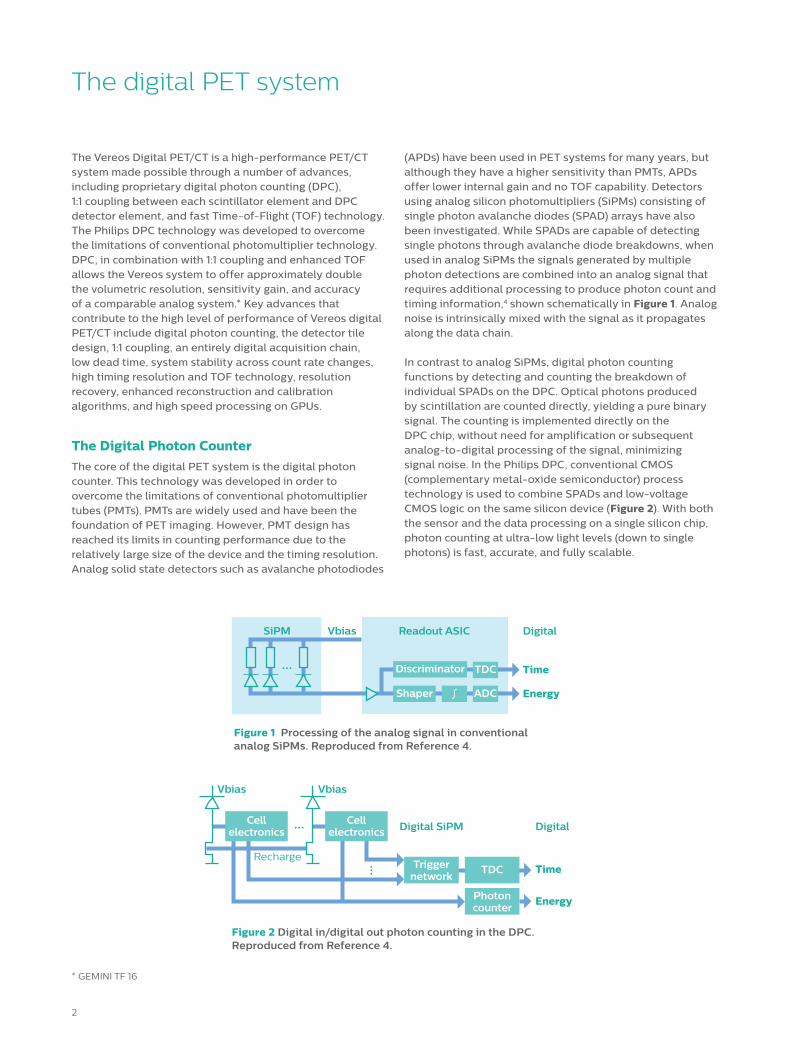
(APDs) have been used in PET systems for many years, but although they have a higher sensitivity than PMTs, APDs offer lower internal gain and no TOF capability. Detectors using analog silicon photomultipliers (SiPMs) consisting of single photon avalanche diodes (SPAD) arrays have alsobeen investigated. While SPADs are capable of detecting single photons through avalanche diode breakdowns, when used in analog SiPMs the signals generated by multiple photon detections are combined into an analog signal that requires additional processing to produce photon count and timing information,4 shown schematically in Figure 1. Analog noise is intrinsically mixed with the signal as it propagates along the data chain.

In contrast to analog SiPMs, digital photon counting functions by detecting and counting the breakdown of individual SPADs on the DPC. Optical photons produced by scintillation are counted directly, yielding a pure binary signal. The counting is implemented directly on the DPC chip, without need for amplification or subsequent analog-to-digital processing of the signal, minimizing signal noise. In the Philips DPC, conventional CMOS (complementary metal-oxide semiconductor) process technology is used to combine SPADs and low-voltage CMOS logic on the same silicon device (Figure 2). With both the sensor and the data processing on a single silicon chip, photon counting at ultra-low light levels (down to single photons) is fast, accurate, and fully scalable.

SiPM Vbias Readout ASIC

Shaper

Discriminator

ADC∫

TDC

Digital

Time

Energy

...

Figure 1 Processing of the analog signal in conventional analog SiPMs. Reproduced from Reference 4.

Vbias Vbias

Digital SiPMCell

electronics

Triggernetwork

Recharge

Digital

Time

Energy

TDC

Photoncounter

Cellelectronics

Figure 2 Digital in/digital out photon counting in the DPC. Reproduced from Reference 4.

* GEMINI TF 16

3

In practice, DPC measurements are made as follows. During a scan, 511 keV photons are converted to scintillation light in the detector crystal. When the first scintillation photon reaches a sensor, the integrated on-chip photon counter increments from 0 to 1, and the integrated timer measures the arrival time. When the second and third scintillation photons are detected by the sensors, the photon counter increments to 2 and 3 respectively (Figure 3). Data acquisition is initiated by a trigger signal, generated when the number of scintillation photons detected in a DPC exceeds the configured trigger threshold. The trigger starts a summing

period and records a timestamp. The photon counter and time are read out at the end of the summing period.

The DPC technology used in the Vereos system takes the form of highly integrated arrays, or tiles, that contain more than 200,000 SPAD cells. Each tile consists of 16 independent die sensors, arranged in a 4 x 4 matrix. Each die sensor consists of four DPC “pixels,” arranged in a 2 x 2 matrix. Each pixel has a photon counter and 3,200 cells. Each die contains a pair of time-to-digital converters, which generate a single timestamp for registered photon detection events.

Microcell

First photon

detected

002

001

0101101101

1 2

3 4

003

Figure 3 Digital photon counting in practice, showing the arrival and detection of individual photons, and timing measurements.

4

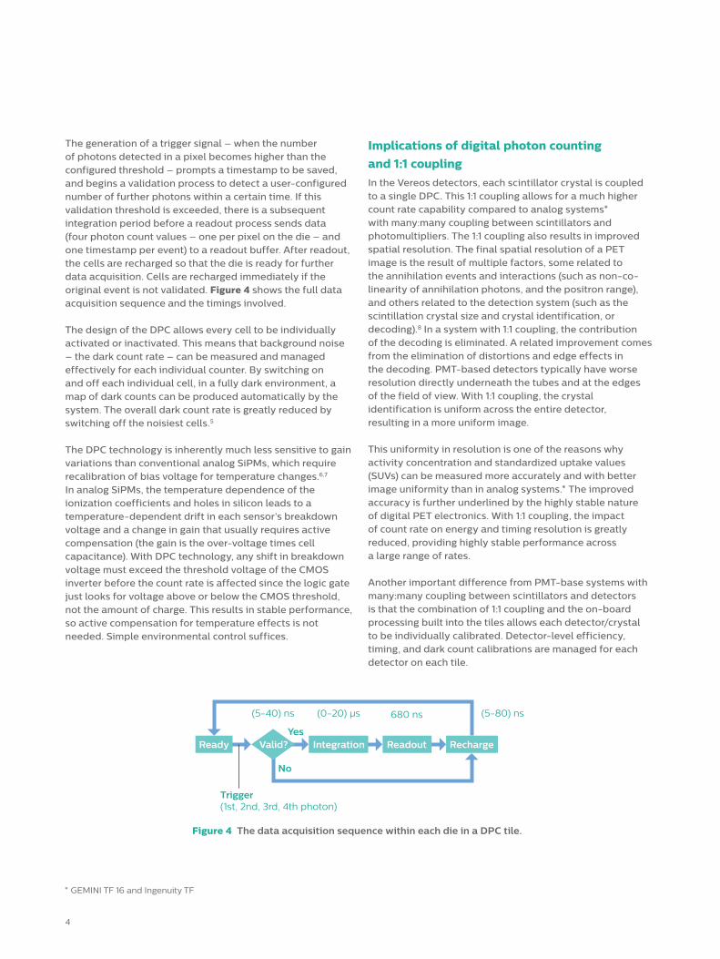
The generation of a trigger signal – when the number of photons detected in a pixel becomes higher than the configured threshold – prompts a timestamp to be saved, and begins a validation process to detect a user-configured number of further photons within a certain time. If this validation threshold is exceeded, there is a subsequent integration period before a readout process sends data (four photon count values – one per pixel on the die – and one timestamp per event) to a readout buffer. After readout, the cells are recharged so that the die is ready for further data acquisition. Cells are recharged immediately if the original event is not validated. Figure 4 shows the full data acquisition sequence and the timings involved.

The design of the DPC allows every cell to be individually activated or inactivated. This means that background noise – the dark count rate – can be measured and managed effectively for each individual counter. By switching on and off each individual cell, in a fully dark environment, a map of dark counts can be produced automatically by the system. The overall dark count rate is greatly reduced by switching off the noisiest cells.5

The DPC technology is inherently much less sensitive to gain variations than conventional analog SiPMs, which require recalibration of bias voltage for temperature changes.6,7 In analog SiPMs, the temperature dependence of the ionization coefficients and holes in silicon leads to a temperature-dependent drift in each sensor’s breakdown voltage and a change in gain that usually requires active compensation (the gain is the over-voltage times cell capacitance). With DPC technology, any shift in breakdown voltage must exceed the threshold voltage of the CMOS inverter before the count rate is affected since the logic gate just looks for voltage above or below the CMOS threshold, not the amount of charge. This results in stable performance, so active compensation for temperature effects is not needed. Simple environmental control suffices.

Implications of digital photon counting and 1:1 couplingIn the Vereos detectors, each scintillator crystal is coupled to a single DPC. This 1:1 coupling allows for a much higher count rate capability compared to analog systems* with many:many coupling between scintillators and photomultipliers. The 1:1 coupling also results in improved spatial resolution. The final spatial resolution of a PET image is the result of multiple factors, some related to the annihilation events and interactions (such as non-co-linearity of annihilation photons, and the positron range), and others related to the detection system (such as the scintillation crystal size and crystal identification, or decoding).8 In a system with 1:1 coupling, the contribution of the decoding is eliminated. A related improvement comes from the elimination of distortions and edge effects in the decoding. PMT-based detectors typically have worse resolution directly underneath the tubes and at the edges of the field of view. With 1:1 coupling, the crystal identification is uniform across the entire detector, resulting in a more uniform image.

This uniformity in resolution is one of the reasons why activity concentration and standardized uptake values (SUVs) can be measured more accurately and with better image uniformity than in analog systems.* The improved accuracy is further underlined by the highly stable nature of digital PET electronics. With 1:1 coupling, the impact of count rate on energy and timing resolution is greatly reduced, providing highly stable performance across a large range of rates.

Another important difference from PMT-base systems with many:many coupling between scintillators and detectors is that the combination of 1:1 coupling and the on-board processing built into the tiles allows each detector/crystal to be individually calibrated. Detector-level efficiency, timing, and dark count calibrations are managed for each detector on each tile.

Ready Integration Readout RechargeValid?

(5-40) ns (0-20) µs 680 ns (5-80) ns

No

Yes

Trigger(1st, 2nd, 3rd, 4th photon)

Figure 4 The data acquisition sequence within each die in a DPC tile.

* GEMINI TF 16 and Ingenuity TF

5

PET performance was evaluated with measurements of energy resolution, TOF resolution, and the NEMA NU 2-2012,9 including spatial resolution, sensitivity, count rate, scatter and image quality. Phantoms and fixtures for system daily QC and from the Philips PET NEMA kit were used for these measurements. Automated analysis was performed using the daily QC procedures and the Philips PET NEMA analysis software available with the system. Measurements were made on multiple systems, including the Vereos digital PET/CT research system installed at The Ohio State University in Columbus, Ohio, USA, and on several preproduction systems built and tested at Philips Advanced Molecular Imaging Research and Development.

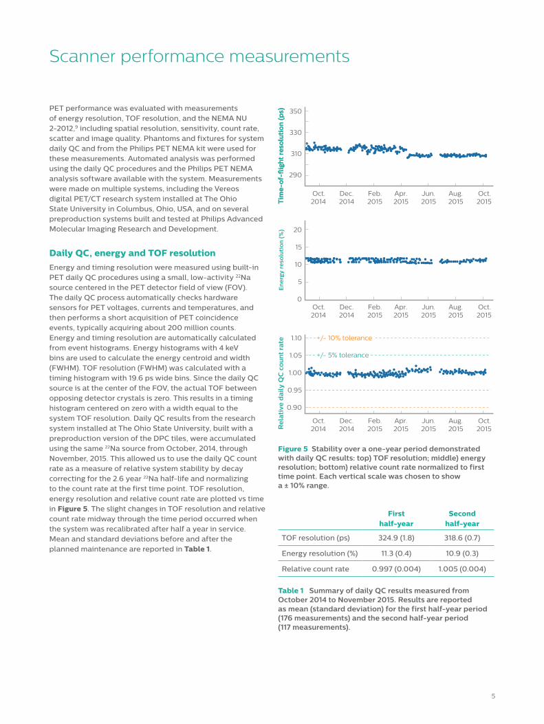
Daily QC, energy and TOF resolution Energy and timing resolution were measured using built-inPET daily QC procedures using a small, low-activity 22Na source centered in the PET detector field of view (FOV). The daily QC process automatically checks hardware sensors for PET voltages, currents and temperatures, and then performs a short acquisition of PET coincidence events, typically acquiring about 200 million counts. Energy and timing resolution are automatically calculated from event histograms. Energy histograms with 4 keV bins are used to calculate the energy centroid and width (FWHM). TOF resolution (FWHM) was calculated with a timing histogram with 19.6 ps wide bins. Since the daily QC source is at the center of the FOV, the actual TOF between opposing detector crystals is zero. This results in a timing histogram centered on zero with a width equal to the system TOF resolution. Daily QC results from the research system installed at The Ohio State University, built with a preproduction version of the DPC tiles, were accumulated using the same 22Na source from October, 2014, through November, 2015. This allowed us to use the daily QC count rate as a measure of relative system stability by decay correcting for the 2.6 year 22Na half-life and normalizing to the count rate at the first time point. TOF resolution, energy resolution and relative count rate are plotted vs time in Figure 5. The slight changes in TOF resolution and relative count rate midway through the time period occurred when the system was recalibrated after half a year in service. Mean and standard deviations before and after the planned maintenance are reported in Table 1.

Scanner performance measurements

First half- year

Second half- year

TOF resolution (ps) 324.9 (1.8) 318.6 (0.7)

Energy resolution (%) 11.3 (0.4) 10.9 (0.3)

Relative count rate 0.997 (0.004) 1.005 (0.004)

Table 1 Summary of daily QC results measured from October 2014 to November 2015. Results are reported as mean (standard deviation) for the first half-year period (176 measurements) and the second half-year period (117 measurements).

Oct. Dec. Feb. Apr. Jun. Aug. Oct.2014 2014 2015 2015 2015 2015 2015

1.10

1.05

1.00

0.95

0.90

Tim

e-o

f-�

igh

t re

solu

tio

n (

ps)

Re

lati

ve d

ail

y Q

C c

ou

nt

rate +/- 10% tolerance

+/- 5% tolerance


20

15

10

5

0

Tim

e-o

f-�

igh

t re

solu

tio

n (

ps)

En

erg

y r

eso

luti

on

(%

)


350

330

310

290

Figure 5 Stability over a one-year period demonstrated with daily QC results: top) TOF resolution; middle) energy resolution; bottom) relative count rate normalized to first time point. Each vertical scale was chosen to show a ± 10% range.

6

Spatial resolutionSpatial resolution was measured as described in NEMA NU2-2012 using glass capillaries containing a small quantity of concentrated 18F at different locations in the PET FOV. The length of the activity in the capillaries (representing a point source) was 2-5 mm. The inside diameter of the capillaries was less than 1 mm. The sources were placed at the ten locations described in NU 2-2012: transverse (x,y) positions (0,1), (0,10), (0,20), (10,0) and (20,0) cm; and axial positions at the center of the axial FOV and three-eighths of the axial FOV length from the center. List-mode PET acquisitions of 10 million events were acquired with the

capillaries parallel to the scanner axis for transverse spatial resolution measurements and perpendicular to the scanner axis for axial spatial resolution measurements. Images were reconstructed from list-mode data sets using a 3D Fourier reprojection algorithm (3D-FRP)10 and an unapodizedfilter.11 Spatial resolution values (full width at half-maximum and tenth-maximum, FWHM and FWTM) were calculated from image profiles through the peak of the source distributions using the procedures outlined in NEMA NU 2-2012. Results are presented in Table 2 and Table 3.

Transverse Tangential Radial

Central 10 cm 20 cm 10 cm 20 cm

FWHM FWTM FWHM FWTM FWHM FWTM FWHM FWTM FWHM FWTM

Mean (mm) 3.99 8.29 4.36 8.79 4.95 10.38 4.64 8.97 5.77 10.26

Standard deviation (mm) 0.10 0.07 0.01 0.03 0.02 0.15 0.03 0.10 0.03 0.03

Table 2 Transverse spatial resolution results from measurements made on two engineering systems. Results were calculated as the mean and standard deviation of four sets of measurements.

Table 3 Axial spatial resolution results from measurements made on two engineering systems.Results were calculated as the mean and standard deviation of three sets of measurements.

Central 10 cm 20 cm

FWHM FWTM FWHM FWTM FWHM FWTM

Mean (mm) 3.99 8.41 4.39 8.74 4.67 9.28

Standard deviation (mm) 0.05 0.04 0.05 0.09 0.02 0.05

7

Transverse Tangential Radial

Central 10 cm 20 cm 10 cm 20 cm

FWHM FWTM FWHM FWTM FWHM FWTM FWHM FWTM FWHM FWTM

Mean (mm) 3.99 8.29 4.36 8.79 4.95 10.38 4.64 8.97 5.77 10.26

Standard deviation (mm) 0.10 0.07 0.01 0.03 0.02 0.15 0.03 0.10 0.03 0.03

OSU system 0 cm

OSU system 10 cm

Eng system 0 cm

Eng system 10 cm

Se

nsi

tivt

y p

er

slic

e (

cps/

kBq

)

0.12

0.08

0.04

0.00

Slice location (mm) -50 0 50

SensitivityThe NEMA NU 2 PET sensitivity was measured using a 700 mm long line source (2 mm ID) containing 2-7 MBq. Measurements were made with the line source along the scanner axis, and with the source offset vertically by 10 cm. List-mode data was acquired at each location while varying the attenuation with a series of five concentric aluminum sleeves. The list data was sorted into sinograms and corrected for randoms. The count rate per source activity was extracted from the sinograms, decay corrected to a

common time, and extrapolated to a zero attenuationvalue, as per NEMA NU 2-2012. TOF effective sensitivity was calculated as the product of NEMA sensitivity and the TOF gain, G = 2D/(c∆t), where D (= 20 cm) is the diameter of the object, c is the speed of light and ∆t is the TOF resolution.12

Sensitivity results are presented in Table 4. Sensitivity profiles are plotted in Figure 6.

Figure 6 Sensitivity profiles measured on an engineering system and the investigational system at OSU.

Figure 7 Plot of true, random and scatter count rates vs activity concentration. Results from seven measurements are shown.

Co

un

t ra

te (

kcp

s)

800

600

400

200

0

Activity concentration (kBq/mL)

Trues

Randoms

Scatter

0 10 20 30 40 50 60

Table 4 Sensitivity results from three engineering systems and the investigational system at OSU. TOF gain for a D = 20 cm object was 4.10 using 325 ps TOF resolution. Results were calculated as the mean (standard deviation) of nine measurements. Due to positioning tolerances and noise, the slight increase in sensitivity at 0 cm is not observed in these results.

LocationSensitivity (cps/kBq)

TOF effective sensitivity (cps/kBq)

0 cm 5.39 (0.31) 22.1 (1.3)

10 cm 5.41 (0.27) 22.2 (1.1)

8

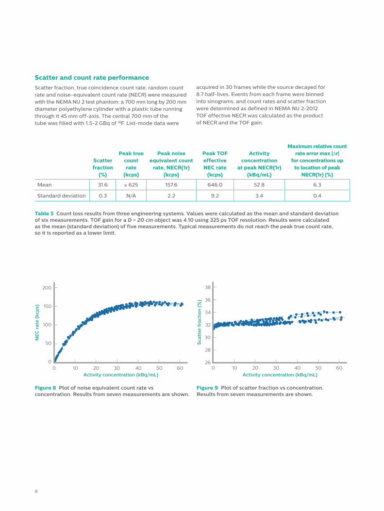
Scatter and count rate performanceScatter fraction, true coincidence count rate, random countrate and noise-equivalent count rate (NECR) were measured with the NEMA NU 2 test phantom: a 700 mm long by 200 mm diameter polyethylene cylinder with a plastic tube running through it 45 mm off-axis. The central 700 mm of the tube was filled with 1.5-2 GBq of 18F. List-mode data were

acquired in 30 frames while the source decayed for 8.7 half-lives. Events from each frame were binned into sinograms, and count rates and scatter fraction were determined as defined in NEMA NU 2-2012. TOF effective NECR was calculated as the product of NECR and the TOF gain.

Table 5 Count loss results from three engineering systems. Values were calculated as the mean and standard deviation of six measurements. TOF gain for a D = 20 cm object was 4.10 using 325 ps TOF resolution. Results were calculated as the mean (standard deviation) of five measurements. Typical measurements do not reach the peak true count rate, so it is reported as a lower limit.

Scatterfraction

(%)

Peak true count rate

(kcps)

Peak noise equivalent count

rate, NECR(1r)(kcps)

Peak TOF effectiveNEC rate

(kcps)

Activity concentration

at peak NECR(1r)(kBq/mL)

Maximum relative count rate error max |∆r|

for concentrations up to location of peak

NECR(1r) (%)

Mean 31.6 ≥ 625 157.6 646.0 52.8 6.3

Standard deviation 0.3 N/A 2.2 9.2 3.4 0.4

Figure 8 Plot of noise equivalent count rate vs concentration. Results from seven measurements are shown.

0 10 20 30 40 50 60

NE

C r

ate

(kc

ps)

200

150

100

50

0

Activity concentration (kBq/mL)

Figure 9 Plot of scatter fraction vs concentration. Results from seven measurements are shown.

Sca

tte

r fr

act

ion

(%

)

38

36

34

32

30

28

26

Activity concentration (kBq/mL)0 10 20 30 40 50 60

9

Image qualityImage quality was assessed by acquiring images of theNEMA/IEC body phantom with hot and cold spheres. The hot spheres were filled with four times the background activity concentration of 5.3 kBq/mL. Hot sphere contrast, QH, cold sphere contrast, QC, and background variability,N, were calculated as defined in the NEMA NU 2 standard. The 2012 revision of NU 2 reduced the acquisition duration for this measurement to about half the duration in the 2007 standard. This reduces the number of counts acquired, and

therefore increases the background variability. To make this change in the standard explicit, scans were acquired with both the NU 2-2012 and NU 2-2007 durations. Results were also calculated from images reconstructed with and without resolution recovery. The results, presented in Table 6 and plotted in Figure 11, show that resolution recovery increases contrast at the cost of also increasing noise. A representative image showing the hot and cold spheres is shown in Figure 10.

Figure 10 Representative image from NEMA NU 2-2012 image quality scans on an engineering system.

10

Figure 11 Plots of contrast (left) and background variability (right) results obtained with and without resolution recover, and with NEMA NU 2-2012 durations (3 minutes, approximately 30 million counts). Points are plotted at the mean. The dashed lines represent the ranges from Table 6. Note that resolution recover increases both contrast and background variability (noise). The default resolution recover settings are intentionally relatively mild. Higher contrast can be obtained, but at the expense of also producing higher noise.

Co

ntr

ast

(%

)

12

10

8

6

4

2

0 10 15 20 25 30 35 40

Without resolution recovery

Dashed lines represent range

With resolution recovery

ROI diameter (mm)

Hot and cold sphere contrast [%] mean (min/max) Background variability [%] mean (min/max)

Duration NU 2- 2012 NU 2- 2007 NU 2- 2012 NU 2- 2007

Resolution recovery

Off On Off On Off On Off On

10 mm30.8

(29.1/33.6)38.5

(34.0/42.9)33.1

(30.9/37.0)40.6

(34.9/47.2)7.2

(6.9/7.4)8.4

(8.1/ 8.7)5.8

(5.6/6.2)6.8

(6.3/7.4)

13 mm48.3

(45.6/49.8)61.3

(57.9/63.3)45.1

(42.5/48.2)56.5

(54.2/58.8)6.1

(6.0/6.2)7.1

(7.1/7.2)4.7

(4.5/5.1)5.6

(5.2/6.0)

17 mm54.1

(50.4/57.1)65.9

(61.1/69.5)52.9

(52.2/53.4)64.1

(63.0/64.7)5.0

(4.7/5.3)5.9

(5.6/6.3)3.7

(3.4/3.9)4.3

(4.0/4.5)

22 mm59.4

(58.8/60.3)68.5

(67.8/69.5)59.9

(58.1/61.3)69.2

(67.0/71.0)4.0

(3.5/4.5)4.6

(4.1/5.3)2.8

(2.6/3.0)3.3

(3.2/3.5)

28 mm79.6

(77.9/81.5)83.4

(81.0/85.7)79.9

(79.0/81.0)83.9

(82.3/85.4)3.1

(2.8/3.6)3.5

(3.1/4.1)2.4

(2.3/2.5)2.7

(2.6/2.8)

37 mm83.5

(82.7/84.3)86.4

(86.0/87.2)83.1

(82.6/84.0)86.4

(85.6/87.3)2.5

(2.3/2.7)2.8

(2.6/3.0)2.0

(1.9/2.1)2.1

(1.9/2.2)

Table 6 Comparison of hot sphere contrast, cold sphere contrast and background variability results obtained with and without resolution recover, and with NEMA NU 2-2012 durations (3 minutes, approximately 30 million counts) and NEMA NU 2-2007 durations (approximately 60 million counts). Results are reported as mean, minimum, and maximum values of three measurements.

Co

ntr

ast

(%

)

100

80

60

40

20

0 10 15 20 25 30 35 40

Hot with resolution recovery

Hot without resolution recovery

Cold with resolution recovery

Cold without resolution recovery

Dashed lines represent range

Sphere inside diameter (mm)

Dia

met

er

11

There are currently no industry-standard methods for assessing PET image uniformity and quantitative accuracy. The closest thing to an existing standard is this statement from the IEC 61675-1 standard for testing PET systems: “No test has been specified to characterize the uniformity of reconstructed images, because all methods known so far will mostly reflect the noise in the image”.13 However, user groups have developed methods for evaluating uniformity and accuracy: notably the American College of Radiology Imaging Network (ACRIN) and the National Cancer Institute’s Centers of Quantitative Imaging Excellence (NCI CQIE).Both use measures of SUV accuracy for site qualification and, where they overlap, have equivalent quantitative criteria. We have adopted the NCI CQIE definitions14 as a starting point towards consistent reporting of uniformity and accuracy. CQIE assessment includes qualitative review of image uniformity and noise characteristics and quantitative review of accuracy of the SUV calibration and the axial variation of average SUV. The Vereos digital PET/CT system exceeds the CQIE and ACRIN criteria for quantitative accuracy and uniformity.

Axial extent Before describing the uniformity metrics, a comment about axial extent is in order. To address the IEC 61675 observation about noise, we have also adopted measures of noise uniformity to complement image uniformity metrics. Measuring noise can be confounded by two factors: theincrease in noise at the edge of the axial field of view due to the shape of the sensitivity profile; and partial volume effects at the edges of phantoms. To provide consistent ways to exclude these types of edge effects, we define two types of axial extent for use in calculating uniformity:the central axial extent, and the useful axial extent. The central axial extent includes image slices that are within the central 40% of the axial coverage and further than 12 mm from the ends of the phantom. The useful axial extent includes slices that are farther than 12 mm from both the ends of the scanner axial coverage and the ends of the active portion of the phantom. These definitions can be applied to images acquired with a single frame images covering the PET detector FOV, for images with longer axial coverage achieved with bed motion and for images acquired using any of the phantoms described by CQIE.14 For our purposes, uniformity measurements are made from images of a 20 cm diameter, 30 cm long water phantom containing a well-mixed 18F solution.

Uniformity metricsVolume averaged SUV, Iva

Accuracy of image intensity is measured with the volume averaged SUV, as defined by CQIE. Circular regions of interest 16 cm diameter are drawn centered on each of the Mu image slices in the useful axial extent, as illustrated in Figure 12. The mean ROI value, xs, is calculated for each slice. The volume averaged SUV is defined as Iva = ∑sxs /Mu.

Axial variation in image intensity, Va

The axial variation in image intensity is calculated as

with the maxima and minima are calculated over the Mu slices in the useful axial extent.

Transverse integral uniformity, IUt

Uniformity in the transverse image planes is assessed using the transverse integral uniformity, IUt. It is calculated from ROI means xs,1...7 obtained from seven circular ROIs as illustrated in Figure 12, drawn on each of the Mc slices in the central 44 mm of the axial coverage. For each of the seven ROIs (i = 1, …, 7), the average over the central 44 mm, yi, is calculated. The range of these averages is used to determine the transverse integral uniformity

with the maxima and minima are calculated over the seven ROIs.

Image uniformity

Va = max (xs ) – min (xs )

mean(xs )

IUt = max (yi ) – min (yi )

max (yi ) + min (yi )

Figure 12 Illustration showing the single 16 cm diameter ROI (left) and the set of seven 6 cm diameter ROIs (right) used for uniformity calculations.

12

10

8

6

4

2

0Act

ivit

y c

on

cen

tra

tio

n (

kBq

/mL

)

-200 -100 0 100 200

Slice location (mm)

VN = max (Ns ) – min (Ns )

N

Mean noise and axial variation of noiseThe “axial variation of noise,” VN, is defined to provide a consistent method for evaluating the extent of noise changes along the axial extent of an image. This metric can be useful for evaluating the impact of non-uniform axial sensitivity profiles such as those encountered with less than 50% bed overlap between frames. The axial variation of noise uses the same seven ROIs as transverse integral uniformity. For each ROI in each of the MCAE slices in the central axial extent, the pixel-wise standard deviation, Si,s, is calculated. The noise for each ROI is defined as Ni,s = si,s /xi,s. The mean noise for each slice is calculated as Ns + ∑iNi,s /7. The mean noise over all slices is defined as N = ∑sNs /MCAE. Then axial variation of noise is defined as

Plots of Ns against slice location provide a visual representation of axial variation of noise, and can facilitate visual detection of abnormal noise-correlation patterns.

A full presentation of uniformity results is outside the scope of this paper. A representative plot of mean activity concentration, xs, is shown in Figure 13.

Figure 13 Mean activity concentration plotted vs slice location from a scan of the 30 cm long uniform cylinder phantom. The image was acquired with the default exam card for PET/CT body imaging.

13

TOF resolution stability

Timing resolution is an important system characteristic for any modern PET system. Excellent TOF resolution is required to provide the well-established benefits of TOF PET.15 Since pulse pile up in the PET detector can affect TOF resolution, it is important to demonstrate TOF resolution stability over the range of count rates. The digital PET design intrinsically minimizes pulse pile up by reducing detector cross talk with 1:1 crystal-to-DPC coupling and by providing a large number of acquisition channels.

Since there is not yet a standardized methodology for assessing TOF resolution stability, two methods were chosen from the literature: one with a “point” source,16 and another with a line source.17 Since the first method uses the digital PET daily QC source, the results are directly comparable to daily QC results reported above. While the line-source method is not directly comparable to the built-in daily QC results, it allows direct comparison to published measurements made on other systems. In the original publications, resolution stability results were presented varying detector singles rate. Singles rate is highly dependent on detector design and only incidentally related to timing resolution stability. To simplify comparisons among systems, singles rates have been converted to net activity in the phantoms.

The point source method is based on the work of Surti et al.18 This measurement used the small daily QC 22Na source placed at the center of the scanner with cylindrical phantoms (20 cm diameter by 30 cm long) placed axially on either side. The cylinders were filled with a large amount of 18F (approximately 0.7 GBq in each phantom) and multiple list-mode data acquisitions were made as the 18F decayed

over 8 half-lives. The long 22Na half-life (2.6 y) left the activity in the small source relatively constant as the 18F decayed. Each event in the list data includes detector position information, photon energy, and TOF. The list-mode data was filtered to exclude events with lines of response passing further than 3.6 cm from the location of the 22Na source in the center of the FOV. TOF resolution measurements from the filtered list files provided a measure of resolution stability across a wide range of count rates.

The second, line-source method is based on the results reported by Jakoby et al.17 In this method, the point source and two cylinder phantoms are replaced with a 40 cm long line source positioned parallel to the scanner axis. The line source was filled with a large amount of 18F (approximately 0.37 GBq) and multiple list-mode data acquisitions were made as the 18F decayed. The list-mode data was filtered to include only events with lines of response perpendicular to the line source. Again, TOF resolution measurements from the filtered list files provided a measure of resolution stability across a wide range of count rates.

TOF resolution stability results from the point source method are shown in Figure 14. There are three things to note in this comparison between the digital and analog PET results. First, the digital detector provides significantly improved time of flight resolution. Second, the 1:1 coupling in the digital system provides much better resolution stability. And finally, the digital system count rate range is considerably larger. A more direct comparison of resolution stability is possible by calculating a relative change in TOF resolution. The relative change is obtained by count rate value, as shown in Figure 15.

Figure 14 TOF resolution measured with the point source method plotted vs net 18F activity in the two cylindrical phantoms. The data plotted with open diamonds is from an analog PET system (Surti et al).

Tim

ing

res

olu

tio

n (

ps

FW

HM

) 1000

800

600

400

200

00.0 0.2 0.4 0.6 0.8 1.0 1.2 1.4

Vereos PET/CTAnalog PET,

JNM 48 (2007) 471

Net 18-F activity (GBq)

Figure 15 Relative change in TOF resolution measured with the point source method plotted vs net 18F activity in the two cylindrical phantoms. The relative change is calculated as the TOF resolution normalized to the low-count-rate value. The data plotted with open diamonds is from an analog PET system (Surti et al).

Re

lati

ve c

ha

ng

e in

tim

ing

re

solu

tio

n 1.6

1.5

1.4

1.3

1.2

1.1

1.0

0.90.0 0.2 0.4 0.6 0.8 1.0 1.2 1.4

Vereos PET/CTAnalog PET, JNM 48 (2007) 471


14

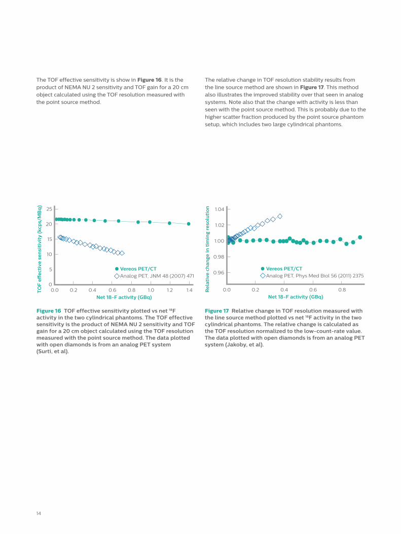
The TOF effective sensitivity is show in Figure 16. It is the product of NEMA NU 2 sensitivity and TOF gain for a 20 cm object calculated using the TOF resolution measured with the point source method.

Figure 16 TOF effective sensitivity plotted vs net 18F activity in the two cylindrical phantoms. The TOF effective sensitivity is the product of NEMA NU 2 sensitivity and TOF gain for a 20 cm object calculated using the TOF resolution measured with the point source method. The data plotted with open diamonds is from an analog PET system (Surti, et al).

TO

F e

�e

ctiv

e s

en

siti

vity

(kc

ps/

MB

q)

25

20

15

10

5

00.0 0.2 0.4 0.6 0.8 1.0 1.2 1.4


Vereos PET/CTAnalog PET, JNM 48 (2007) 471

Figure 17 Relative change in TOF resolution measured with the line source method plotted vs net 18F activity in the two cylindrical phantoms. The relative change is calculated as the TOF resolution normalized to the low-count-rate value. The data plotted with open diamonds is from an analog PET system (Jakoby, et al).

Re

lati

ve c

ha

ng

e in

tim

ing

re

solu

tio

n 1.04

1.02

1.00

0.98

0.96

0.0 0.2 0.4 0.6 0.8


Vereos PET/CTAnalog PET, Phys Med Biol 56 (2011) 2375

The relative change in TOF resolution stability results from the line source method are shown in Figure 17. This method also illustrates the improved stability over that seen in analog systems. Note also that the change with activity is less than seen with the point source method. This is probably due to the higher scatter fraction produced by the point source phantom setup, which includes two large cylindrical phantoms.

15

Dead time

One of the important characteristics of the DPC detector system is very low dead time. The DPC acquisition chain has two orders of magnitude more acquisition channels than analog PET systems,* resulting in lower throughput per channel and low dead time. Figure 18 shows a comparison of dead time measured on the Vereos system and an analog PET system.* Dead time was measured on both systems by monitoring the decay of an 18F-filled water phantom (30 cm long, 20 cm diameter) for multiple half-lives. The Vereos system demonstrates very good dead-time performance with only an approximate 34% loss at the very high activity concentration of 70 kBq/mL. The count rates and dead time observed at 70 kBq/mL with this phantom are similar to those obtained when simulating one of the highest dose procedures currently in use: cardiac imaging with 82Rb. The SNMMI/ACNC/SCCT guideline for PET myocardial perfusion imaging with 82Rb lists a standard tracer dose of 1.5-2.2 GBq for systems such as Vereos.19 Measurements made with 1.4 GBq 18F boluses based on 82Rb biodistribution data from Senthamizhchelvan et al.20 produced peak dead time correction factors similar to those shown in the Vereos data in Figure 18.

Figure 18 Comparison of dead time correction factors measured on Vereos digital PET and analog PET (Ingenuity TF).

Vereos digital PETAnalog PET

0 10 20 30 40 50 60 70

De

ad

tim

e c

orr

ecti

on

fa

cto

r

3.0

2.5

2.0

1.5

1.0

Calibration activity concentration (kBq/mL)

Discussion

This paper has described the Vereos digital PET/CT and presented a broad range of PET performance measurements. The breadth of performance values is necessary because no single parameter can fully describe a system and its suitability for a particular application. For example, sensitivity directly impacts the number of counts collected. Decisions about how many counts to acquire requires balancing the desired image quality, acquisition duration and activity. But sensitivity is not entirely a clinically relevant measurement. NEMA sensitivitymeasurements are designed to be made in the absence of random and scatter events, with no dead time and minimal attenuation: it does not include the effect of the most important corrections. Count loss measurements cover rate-dependent effects like random events and dead

time, but do not reflect the improvements afforded by TOF, which impacts image quality by improving convergence and signal to noise. Spatial resolution impacts contrast and quantitative accuracy, as do TOF and choice of reconstruction parameters. This interplay among systemcharacterization data must be taken into account when considering how a system supports any particular use. Vereos has been designed to provide excellent NEMA NU 2 performance values, with exceptional TOF resolution, and with the premium stability and uniformity. Combined, this provides two-fold improvements over the GEMINI TF PET/CT: in the TOF gain and reduced dead time; in volumetric resolution, and the quantitative accuracy as measured using the NCI CQIE criteria.

* Ingenuity TF

References

1. Degenhardt C, et al. The digital silicon photomultiplier - a novel sensor for the detection of scintillation light. Nuclear Science Symposium Conference Record (NSS/MIC). IEEE 2009.

2. Degenhardt C, et al. Arrays of digital silicon photomultipliers - intrinsic performance and application to scintillator readout. Nuclear Science Symposium Conference Record (NSS/MIC). IEEE 2010.

3. Philips Healthcare. Truly digital PET imaging: Philips proprietary Digital Photon Counting technology. 2016: Eindhoven, The Netherlands.

4. Frach T, Prescher G, and Degenhardt C. Silicon photomultiplier technology goes fully digital. Electronic Engineering Times Europe. 2010.

5. Haemisch Y, et al. Fully digital arrays of silicon photomultipliers (dSiPM) – a scalable alternative to vacuum photomultiplier tubes (PMT). Physics Procedia. 2012;37:1546–1560.

6. Frach T, et al. The digital silicon photomultiplier – principle of operation and intrinsic detector performance. Nuclear Science Symposium Conference Record (NSS/MIC). IEEE 2009.

7. Musienko Y. State of the art in SiPM’s, in industry-academia matching event on SiPM and related technologies. CERN 2011.

8. Derenzo SE and Moses WW. Critical instrumentation issues for resolution <2mm, high sensitivity brain PET, in quantification of brain function: tracer kinetics and image analysis in brain PET: proceedings of PET ’93 Akita. Quantification of Brain Function, Uemura K, Editor 1993, Elsevier: Akita, Japan. 25–40.

9. NEMA NU 2-2012. Performance Measurements of Positron Emission Tomographs. National Electrical Manufacturers Association Rosslyn, VA. 2013.

10. Matej S and Kazantsev IG. Fourier-based reconstruction for fully 3-D PET: Optimization of interpolation parameters. Medical Imaging, IEEE Transactions on. 2006;25(7):845–854.

11. Matej S and Lewitt RM. 3D-FRP: direct Fourier reconstruction with Fourier reprojection for fully 3-D PET. Nuclear Science, IEEE Transactions on. 2001;48(4):1378–1385.

12. Budinger TF. Time-of-flight positron emission tomography: status relative to conventional PET. Journal of Nuclear Medicine. 1983;24(1):73–8.

13. International Electrotechnical Commission, IEC 61675-1 Radionuclide imaging devices – Characteristics and test conditions – Part 1: Positron emission tomographs. International Electrotechnical Commission: Geneva. 2013.

14. NCI Centers of Quantitative Imaging Excellence, Manual of Procedures Part D: PET/CT Technical Procedures, v 3.2, 2013, ACRIN/NCI CQIE.

15. Daube-Witherspoon ME et al. Determination of Accuracy and Precision of Lesion Uptake Measurements in Human Subjects with Time-of-Flight PET. Journal of Nuclear Medicine. 2014;55:1–6.

16. Surti S, et al. Performance of Philips GEMINI TF PET/CT scanner with special consideration for its time-of-flight imaging capabilities. Journal of Nuclear Medicine. 2007;48(3):471–80.

17. Jakoby BW, et al. Physical and clinical performance of the mCT time-of-flight PET/CT scanner. Physics in Medicine and Biology. 2011;56(8):2375–89.

18. Surti S, et al. Impact of time-of-flight PET on whole-body oncologic studies: a human observer lesion detection and localization study. Journal of Nuclear Medicine. 2011;52(5):712–9.

19. Dorbala S, et al. SNMMI/ASNC/SCCT Guideline for Cardiac SPECT/CT and PET/CT 1.0. Journal of Nuclear Medicine. 2013;54(8):1485–507.

20. Senthamizhchelvan S, et al. Human biodistribution and radiation dosimetry of 82Rb. Journal of Nuclear Medicine. 2010;51(10):1592–9.

Results in this white paper are from research and engineering systems. Product specifications may vary.

© 2016 Koninklijke Philips N.V. All rights are reserved.Philips reserves the right to make changes in specifications and/or to discontinue any product at any time without notice or obligation and will not be liable for any consequences resulting from the use of this publication. Trademarks are the property of Koninklijke Philips N.V. or their respective owners.

www.philips.com/VereosPETCT

Printed in The Netherlands.4522 991 19831 * JUN 2016

focusing on imaging high performance vereos pet/ct

Documents