Flying into the Future: AviationEmissions Scenarios to 2050B E T H A N O W E N , * D A V I D S . L E E , A N DL I N G L I M

Dalton Research Institute, Manchester MetropolitanUniversity, John Dalton Building, Chester Street,Manchester M1 5GD, United Kingdom

Received August 19, 2009. Revised manuscript receivedJanuary 13, 2010. Accepted February 14, 2010.

This study describes the methodology and results forcalculating future global aviation emissions of carbon dioxideand oxides of nitrogen from air traffic under four of the IPCC/SRES (Intergovernmental Panel on Climate Change/SpecialReport on Emissions Scenarios) marker scenarios: A1B, A2, B1,and B2. In addition, a mitigation scenario has been calculatedfor the B1 scenario, requiring rapid and significant technologydevelopment and transition. A global model of aircraft movementsand emissions (FAST) was used to calculate fuel use andemissions to 2050 with a further outlook to 2100. The aviationemission scenarios presented are designed to interpret the SRESand have been developed to aid in the quantification of theclimate change impacts of aviation. Demand projections aremade for each scenario, determined by SRES economic growthfactors and the SRES storylines. Technology trends areexamined in detail and developed for each scenario providingplausible projections for fuel efficiency and emissionscontrol technology appropriate to the individual SRES storylines.The technology trends that are applied are calculated frombottom-up inventory calculations and industry technology trendsand targets. Future emissions of carbon dioxide are projectedto grow between 2000 and 2050 by a factor in the range of2.0 and 3.6 depending on the scenario. Emissions of oxides ofnitrogen associated with aviation over the same period areprojected to grow by between a factor of 1.2 and 2.7.

IntroductionAviation currently contributes between 2 and 3% of totalannual anthropogenic carbon dioxide (CO2) emissions (1)but possibly as much as 4.9% of radiative forcing in 2005,including cirrus cloud effects (2). Aviation has grown stronglyover recent decades with passenger transport in terms ofrevenue passenger kilometers (RPK) increasing at an averagerate of 5.2% yr-1 over the period 1992-2005, despite world-changing events such as the first and second Gulf Wars andthe World Trade Center attack, etc. (2). The future potentialgrowth of emissions from this sector is of some concern sinceits impacts on climate arise from both CO2 and non-CO2

emissions and effects. Moreover, international aviationemissions which contribute approximately 60% of the totalare not part of the Kyoto Protocol and lie outside the remitof internationally agreed emission reduction targets. Eventhough there have been significant improvements in fuelefficiency through aircraft technology and operational man-agement this has been outweighed by the increase in airtraffic.

Previously, some efforts have been made to formulatefuture aviation emissions scenarios (3) but these are nowover 10 years old and were based on older IPCC scenarioassumptions. Here, we present new aviation emissionscenarios to 2050 that are designed to interpret the IPCCSRES storylines (4) under the four main families A1B, A2, B1,and B2 with a further outlook to 2100. In addition, a scenariohas been calculated assuming that the ambitious technologytargets of the Advisory Council for Aeronautical Research inEurope (ACARE) (5) are achieved. The emission scenariospresented here are time-variant and have been gridded sothat impacts can be assessed with climate models includingchemical transport models (CTMs). These aviation emissionsscenarios form part of the European Commission sixthFramework project ‘QUANTIFY’, in which SRES-based emis-sion scenarios have been developed in a consistent mannerfor the transportation sector as a whole (www.pa.op.dlr.de/quantify/).

Calculation of Baseline Fuel and Emissions

A global model of aircraft movements and emissions, ‘FAST’(6), for a baseline year of 2000 has been used as the basis forcalculation of new future emissions for scenario years 2020,2050, and 2100 under the SRES marker scenarios (A1B, A2,B1, and B2). FAST has previously been used to calculate fuel,CO2 and NOx emissions for aviation and used in a variety ofimpact studies (7-10) and is also in use under the aegis ofthe International Civil Aviation Organization (ICAO)’s Com-mittee on Aviation Environmental Protection (CAEP), alongwith other similar modeling systems. The emission scenariosare spatially resolved at 1° latitude × 1° longitude with avertical discretization of 610 m (i.e., flight-level intervals of2000 feet), every month. FAST combines a global aircraftmovements database of scheduled and nonscheduled airtraffic (11) with data on fuel flow provided by a separatecommercial aircraft performance model, PIANO (12). Emis-sions of CO2 are a simple function of fuel consumption,whereas NOx emissions require an algorithm that correctscertification (ICAO databank) data for altitude (13, 14). Globalaviation fuel from civil aviation using FAST was calculatedto be 152 Tg for 2000. This is in broad agreement with otherestimates of emissions (15, 16). The fuel burn derived from“bottom-up” inventories such as the FAST2000 inventorygenerally indicate lower fuel use than reported aviation fueluse by the International Energy Agency (IEA) (17). There area number of reasons for this. First, the “bottom-up”inventories only indicate civil emissions, military emissionsare much more difficult to estimate but Eyers et al. (15)calculated this to be approximately 11% of the total in 2002.

Second, many of these inventories including FAST2000are idealized in terms of missions, in that great circle distancesare assumed and no holding patterns. This leads to anunderestimate of actual burn of about 10% (15). These variousfactors conspire to systematically underestimate aviation CO2

emissions, which is why it is important to use the total fuelsales data and the more detailed bottom-up inventory totalshould be scaled accordingly. In this study the FAST2000data has been normalized to the IEA total aviation fuel salesfigure of 214 Tg yr-1 for 2000. This method of scaling to IEAfuel, while conventional (3), introduces some uncertainty inthe location (both horizontally and vertically) of the NOx

emissions. In particular, military emissions will be emittedat different altitudes to civil aviation and a CTM user mayconsequently choose to omit the military portion of NOx

from their calculations. However, the uncertainties intro-* Correpsonding author e-mail: B.Owen@mmu.ac.uk.

Environ. Sci. Technol. 2010, 44, 2255–2260

10.1021/es902530z 2010 American Chemical Society VOL. 44, NO. 7, 2010 / ENVIRONMENTAL SCIENCE & TECHNOLOGY 9 2255

Published on Web 03/12/2010

duced by scaling of the fuel use data are not significant forCO2 emissions.

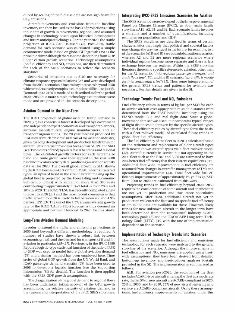
Aircraft movements and emissions from the baselineinventory can then be used as the basis of projections, usinginput data of growth in movements (regional) and assumedchanges in technology based upon historical developmentand future anticipated changes. For the year 2020, the trafficprojection of ICAO/CAEP is used (18). Post-2020, trafficdemand for each scenario was calculated using a simpleeconometric model based on global GDP growth (19) as theprinciple driver although there is some decoupling from GDPunder certain growth scenarios. Technology assumptions(on fuel efficiency and NOx emissions) are then determinedfor each of the SRES scenarios to reflect the scenariostorylines.

Scenarios of emissions out to 2100 are necessary forclimate-response type calculations (20) and were developedfrom the 2050 scenarios. Uncertainty increases beyond 2050which renders overly complex assumptions difficult to justify.Demand up to 2100 is modeled as described as for the period2020-2050 but more simple technology assumptions weremade and are provided in the scenario descriptions.

Aviation Demand in the Near-Term

The ICAO projection of global aviation traffic demand to2020 (18) is a consensus forecast developed by Governmentand independent expert economists and transport planners,airframe manufacturers, engine manufacturers, and airtransport organizations. The 20 year forecast produced byICAO is very much “in view” in terms of the aviation industry,given the long development and production timeframes foraircraft. This forecast provides a breakdown of RPK and SKO(seat kilometers offered) by aircraft seat bandings and regionalflows. The calculated growth factors for each aircraft sizeband and route group were then applied to the year 2000baseline inventory activity data, producing an aviation activitydata set for 2020. The overall global growth in SKO shownby the ICAO forecast is 4.1% yr-1 until 2020. In terms of aircrafttypes, an upward trend in the size of aircraft making up theglobal fleet is projected by the Forecasting and EconomicSub-Group (FESG) with aircraft of more than 300 seatscontributing to approximately 11% of total SKOs in 2002 and18% in 2020. The ICAO/FESG has recently completed a newforecast to 2026 (21) and the most recent consensus is thattraffic growth to 2026 is likely to fall between 4.2 and 4.9%per year (22, 23). The use of the 4.3% annual average growthrate of the ICAO/CAEP6-FESG forecast is thus deemed anappropriate and pertinent forecast to 2020 for this study.

Long-Term Aviation Demand Modeling

In order to extend the traffic and emissions projections to2050 (and beyond) a different methodology is required. Anumber of studies have shown a robust link betweeneconomic growth and the demand for transport (24) and foraviation in particular (25-27). Previously, in the IPCC 1999Report a logistic-type statistical function of the ratio of RPKto GDP was used to model future global aviation demand(28) and a similar method has been employed here. Timeseries of global GDP growth from the UN World Bank andICAO passenger demand statistics (29) have been used to2006 to develop a logistic function (see the SupportingInformation (SI) for details). The function is then appliedwith the SRES GDP growth assumptions.

The disaggregation of the global demand to regional flowshas been undertaken taking account of the GDP growthassumptions, the relative maturity of aviation demand inthe regions and interpretation of the IPCC SRES storylines.

Interpreting IPCC-SRES Emissions Scenarios for AviationThe SRES scenarios were developed by the IntergovernmentalPanel on Climate Change (IPCC), as four main familystorylines: A1B, A2, B1, and B2. Each scenario family involvesa storyline and a number of quantifications, includingestimates on population and GDP.

The SRES storylines are described in terms of certaincharacteristics that imply that political and societal factorsmay change the way we travel in the future; for example, twoof the scenarios (A1B and B1) are both globalization scenarios,whereas A2 and B2 are more regional scenarios whereindividual regions become more separate and there is lessexchange between the regions. Within the SRES storylineliterature there is no specific reference to aviation, other thanfor the A2 scenario: “interregional passenger transport andtrade flows low” (30); and the B1 scenario: “air traffic is mostlyfor intercontinental trips” (31). Thus some interpretation ofthe general SRES trends and patterns for aviation wasnecessary. Further details are given in the SI.

Technology Trends: Fuel and NOx EmissionsFuel efficiency values in terms of kg fuel per SKO for eachin-service aircraft over appropriate mission distances weredetermined from the FAST baseline inventory using thePIANO model (12) and real flight data. Since a globalmovement data set was used, it incorporates typical rangesof flight distances undertaken by the specific aircraft types.These fuel efficiency values by aircraft type form the basis,with a fleet-rollover model, of calculated future trends inglobal fleet fuel efficiency.

The fuel efficiency of the fleet to 2020 is calculated basedon the retirement and replacement of older aircraft typeswith newer known aircraft types via a fleet rollover model(32). Aircraft currently in-service but not appearing in the2000 fleet such as the B787 and A380 are estimated to have20% better fuel efficiency that their current equivalents (33).Additional fleet-wide improvements in fuel efficiency areassumed from changes in air traffic management (ATM) andoperational improvements (34). Total fleet-wide fuel ef-ficiency improvements of approximately 1% yr-1 as kg/SKOfrom 2000 to 2020 are estimated from this work.

Projecting trends in fuel efficiency beyond 2020-2050requires the consideration of some aircraft and engines thatare not yet in production and thus more speculativeassumptions. After 2020, additional aircraft not yet inproduction will enter the fleet and no specific fuel efficiencyor emissions data are available for these. However, likelytrends for new unknown aircraft in the longer term havebeen determined from the aeronautical industry ACAREtechnology goals (5) and the ICAO/CAEP Long-term Tech-nology Goals (LTTG) (35) with the rate of implementationdependent on the scenario.

Implementation of Technology Trends into ScenariosThe assumptions made for fuel efficiency and emissionstechnology for each scenario were matched to the generalstoryline of the scenarios. Although the improvements infuel efficiency and NOx emissions are applied using fleet-wide assumptions, they have been derived from detailedbottom-up inventory and fleet-rollover analyses (detailsprovided in the SI). The implementation is summarized asfollows:

A1B. For aviation post-2020, the evolution of the fleetincludes ACARE-type aircraft entering the fleet at a moderaterate, that is, 5% of new aircraft are ACARE-compliant in 2020,25% in 2030, and by 2050, 75% of new aircraft entering intoservice are ACARE-compliant aircraft. Using these assump-tions, fuel efficiency improvements for aviation under this

2256 9 ENVIRONMENTAL SCIENCE & TECHNOLOGY / VOL. 44, NO. 7, 2010

scenario were assumed to be approximately 1% yr-1 for theentire 50 year period (2000-2050). This matches the rate offuel efficiency improvements seen in the industry over thepast 10 years but this rate of improvement is assumed to besustained to 2050 which is a generally optimistic outcomeand consistent with the A1 storyline of technological im-provement (previous future projections of fuel efficiency haveassumed a declining rate of improvement with time, forexample, IPCC projections assumed efficiency improvementswould decline to 0.5% yr-1 post-2020-2100) (28). Improve-ments in NOx technology under the A1 scenario are signifi-cant, commensurate with the generally high level of tech-nological advancement and exchange. It is thus assumedthat the medium term technology targets proposed by theCAEP are implemented by 2030 and achieved by all newaircraft entering the fleet after 2030.

A2. This scenario has the lowest overall demand and thelack of technological advances and international cooperationmean that the step-changes that would be required to developACARE-type aircraft are not achieved and fuel efficiencyimprovements after 2020 are slow, amounting to an overallimprovement of 30% over 2000 values by 2050. Only marginalannual improvements in fuel efficiency (0.2% yr-1 post-2020-2100) and NOx emissions technology are assumed.

B1. For this scenario, where local air quality would be animportant driver for reducing NOx emissions, significantimprovements in NOx technology are assumed, commen-surate with achieving the long-term technology goals for NOx

proposed within CAEP and the ACARE NOx improvementsdiscussed by the aeronautical industry. Fuel efficiencyimprovements are based on the same assumption outlined

for the A1 scenario to 2050 (1% yr-1 in kg/SKO) but increaseagain to 1.3% yr-1 (kg/SKO) in the period 2020-2100 as thepossibility of more radical aircraft design and materials andalternative fuels become available. As with all the scenarios,for the period 2050-2100, the fuel efficiency improvementsare speculative and top-down. The B1-ACARE scenario sharesthe same EINOx assumptions as B1 but with the fuel efficiencyassumptions tightened further by assuming that the ACAREfuel efficiency goal is achieved by all new aircraft enteringthe fleet in 2020 (a 2.1% yr-1 improvement in kg/SKO). Thisscenario is effectively a parametric “what if”, since it is clearthat the ACARE targets are demanding, and it would bevirtually impossible for all newly manufactured aircraft tomeet the targets since this would require existing types to bere-engined; rather, in reality, ACARE opportunities only existfor new aircraft types. For the B1-ACARE scenario, post-2050, the rate of fuel efficiency obtained up to 2050 wouldbe continued to 2100. The B1-ACARE scenario is akin to anaviation mitigation scenario as to achieve the fuel efficiencyimprovements described here, would probably require thetechnology to be driven by concerns over climate change.However, it should be noted that the B1 SRES total emissionsscenario is not a mitigation scenario and has a 2100temperature increase of around 2.6 °C in excess of the levelcommonly associated with “dangerous climate change” (36).

B2. The B2 scenario also shows some ecological creden-tials although with environmental policies being prominentonly at a local level, the implementation of tougher NOx

emission standards through groups such as ICAO/CAEP areassumed to be less likely. The B2 scenario also lacks thetechnological advances evident in the B1 world. The B2

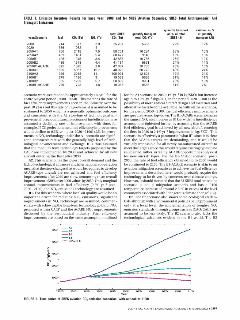
FIGURE 1. Time series of SRES aviation CO2 emission scenarios (with outlook to 2100).

TABLE 1. Emission Inventory Results for base year, 2000 and for SRES Aviation Scenarios; SRES Total Anthropogenic; AndTransport Emissions

year/Scenario fuel CO2 (Tg) NOx (Tg)total SRES

CO2 (Tg)quantify transport

total CO2 (Tg)

quantify transportas % of total

SRES (5)

aviation as %of quantify

transport (38)

2000 214 677 2.9 25 287 5665 22% 12%2020 336 1062 42050A1 766 2418 7.5 58 701 16 284 28% 15%2050A2 469 1481 5.4 60 472 9148 15% 16%2050B1 426 1345 3.4 42 887 10 785 25% 12%2050B2 435 1373 4.4 41 194 9861 24% 14%2050B1ACARE 325 1025 2.6 42 887 10 785 25% 10%2100A1 1605 5067 15.7 48 020 20 773 43% 24%2100A2 956 3018 11 105 991 12 803 12% 24%2100B1 375 1186 3 19 053 9656 51% 12%2100B2 565 1783 5.7 50 689 9951 20% 18%2100B1ACARE 229 723 1.8 19 053 9656 51% 7%

VOL. 44, NO. 7, 2010 / ENVIRONMENTAL SCIENCE & TECHNOLOGY 9 2257

scenario is thus characterized by fairly slow improvementsin NOx technology between 2020 and 2050. Modest im-provements in fuel efficiency similar to those used in theIPCC scenarios (28) of 1% yr-1 to 2030 and 0.6% yr-1 to 2050(and then to 2100) are assumed.

RESULTSEmission Scenarios to 2050. Global emissions of CO2 andNOx according to the methodology described above aresummarized in Table 1. For the B1 scenario there is also aB1-ACARE variant (an aviation advanced technology sce-nario) which assumes more significant improvements in fuelefficiency. The projected trends over time of aviation CO2

and NOx emissions for each of the scenarios is shown inFigure 1. For the high growth A1 scenario, emissions of CO2

grow by an average of 2.6% yr-1. Emissions of NOx for theA1 scenario grow by an average of 2.0% yr-1. The B1-ACAREscenario represents a future with a more environmental

outlook where demand is slower and fuel efficiency and NOx

technology improvements are both stronger. The emissionsof CO2 grow by an average of 0.8% yr-1 between 2000 and2050. Emissions of NOx for the B1-ACARE scenario declineby an average of 0.1% yr-1 between 2000 and 2050 as a resultof the combined improvements of fuel savings and NOx

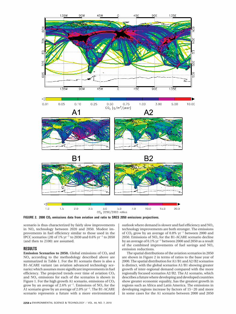
emission reductions.The spatial distributions of the aviation scenarios in 2050

are shown in Figure 2 in terms of ratios to the base year of2000. The spatial distribution for A1/B1 and A2/B2 scenariosis distinct, with the global scenarios A1/B1 showing greatergrowth of inter-regional demand compared with the moreregionally focused scenarios A2/B2. The A1 scenario, whichdescribes a future where developing and developed countriesshow greater economic equality, has the greatest growth inregions such as Africa and Latin America. The emissions indeveloping regions increase by factors of 15-20 and morein some cases for the A1 scenario between 2000 and 2050

FIGURE 2. 2000 CO2 emissions data from aviation and ratio to SRES 2050 emissions projections.

2258 9 ENVIRONMENTAL SCIENCE & TECHNOLOGY / VOL. 44, NO. 7, 2010

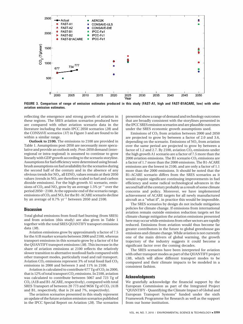
reflecting the emergence and strong growth of aviation inthese regions. The SRES aviation scenarios produced hereare compared with other aviation scenario data in theliterature including the main IPCC 2050 scenarios (28) andthe CONSAVE scenarios (37) in Figure 3 and are found to liewithin a similar range.

Outlook to 2100. The emissions to 2100 are provided inTable 1. Assumptions post-2050 are necessarily more specu-lative and provide an outlook only. Post-2050 demand (inter-regional or intra-regional) is assumed to continue to growlinearly with GDP growth according to the scenario storyline.Assumptions for fuel efficiency were determined using broad-brush assumptions on fuel availability for the scenarios duringthe second half of the century and in the absence of anyobvious trends for NOx, all EINOx values remain at their 2050values (trends in NOx are therefore scaled to fuel and carbondioxide emissions). For the high growth A1 scenario, emis-sions of CO2 and NOx grow by an average 1.5% yr-1 over theperiod 2050-2100. At the opposite end of the scenario range,emissions of CO2 and NOx for the B1-ACARE scenario declineby an average of 0.7% yr-1 between 2050 and 2100.

DiscussionTotal global emissions from fossil fuel burning (from SRES)and from aviation (this study) are also given in Table 1together with the total SRES QUANTIFY transport emissionsdata (38).

Aviation emissions grow by approximately a factor of 7.5for the A1B marker scenario between 2000 and 2100, whereastransport emissions in this scenario grow by a factor of 4 forthe QUANTIFY transport emissions (38). This increase in theshare of aviation emissions at 2100 reflects the relativelyslower transition to alternative nonfossil fuels compared withother transport modes, particularly road and rail transport.Aviation CO2 emissions represent 3% of total fossil fuel CO2

emissions in 2000 and between 3 and 11% in 2100.Aviation is calculated to contribute 677 Tg of CO2 in 2000,

that is 12% of total transport CO2 emissions. In 2100, aviationwas calculated to contribute between 5067 and 723 Tg ofCO2 (A1B and B1-ACARE, respectively), compared with totalSRES Transport of between 20 773 and 9656 Tg of CO2 (A1Band B1, respectively, that is 24 and 7%, respectively).

The aviation scenarios presented in this study representan update of the future aviation emission scenarios publishedin the IPCC Special Report on Aviation (28). The scenarios

presented show a range of demand and technology outcomesthat are broadly consistent with the storylines presented inthe IPCC SRES emission scenarios and are plausible outcomesunder the SRES economic growth assumptions used.

Emissions of CO2 from aviation between 2000 and 2050are projected to grow by between a factor of 2.0 and 3.6,depending on the scenario. Emissions of NOx from aviationover the same period are projected to grow by between afactor of 1.2 and 2.7. By 2100, aviation CO2 emissions underthe high growth A1 scenario are a factor of 7.5 more than the2000 aviation emissions. The B1 scenario CO2 emissions area factor of 1.7 more than the 2000 emissions. The B1-ACAREemissions are the lowest in 2100, and are only a factor of 1.1more than the 2000 emissions. It should be noted that theB1-ACARE scenario differs from the SRES scenarios as itwould require significant continuing improvements in fuelefficiency and some radical technological advances in thesecond half of the century probably as a result of some climateconcerns and policy. Moreover, we have implementedachievement of ACARE targets for all newly manufacturedaircraft as a “what if”, in practice this would be impossible.

The SRES scenarios by design do not include mitigationpolicies for climate change. If emissions from internationalaviation remain outside emission reduction targets set forclimate change mitigation the aviation emissions presentedhere may occur while emissions from other sectors are rapidlyreduced. Emissions from aviation would thus become fargreater contributors in the future to global greenhouse gasemissions and climate change. While aviation is not currentlyone of the main drivers of global warming, the growthtrajectory of the industry suggests it could become asignificant factor over the coming decades.

The SRES scenarios have been interpreted for aviationwith other transport modes as part of the QUANTIFY project(38), which will allow different transport modes to becompared and their climate impacts to be modeled in aconsistent fashion.

AcknowledgmentsWe gratefully acknowledge the financial support by theEuropean Commission as part of the Integrated Project“QUANTIFY - Quantifying the Climate Impact of Global andEuropean Transport Systems” funded under the sixthFramework Programme for Research as well as the supportfrom our home institution.

FIGURE 3. Comparison of range of emission estimates produced in this study (FAST-A1, high and FAST-B1ACARE, low) with otheraviation emission estimates.

VOL. 44, NO. 7, 2010 / ENVIRONMENTAL SCIENCE & TECHNOLOGY 9 2259

Supporting Information AvailableDetails on modeling the traffic demand for the SRESstorylines, a description of the SRES scenarios and furtherdetails on projecting future emission trends. This materialis available free of charge via the Internet at http://pubs.acs.org.

Literature Cited(1) IEA. CO2 Emissions from Fuel Combustion 1971-2001; Inter-

national Energy Agency Organisation for Economic Co-Opera-tion and Development: Paris, 2007.

(2) Lee, D. S.; Fahey, D. W.; Forster, P. M.; Newton, P. J.; Wit, R. C. N.;Lim, L. L.; Owen, B.; Sausen, R. Aviation and global climatechange in the 21st century. Atmos. Environ. 2009, 43, 3520–3537.

(3) IPCC. Aviation and the Global Atmosphere. In IntergovernmentalPanel on Climate Change; Penner, E. Lister J., Griggs, D. H.,Dokken, D. J., McFarland M., D. J., Eds.; Cambridge UniversityPress: Cambridge, UK, 1999.

(4) IPCC. Special Report on Emission Scenarios Working Group IIIof the Intergovernmental Panel on Climate Change; CambridgeUniversity Press: Cambridge, UK, 2000.

(5) ACARE. Strategic Research Agenda; Advisory Council for Aero-nautics Research in Europe: Brussels, 2002; Vol. 2.

(6) Lee D. S.; Owen B.; Graham A.; Fichter C.; Lim L. L.; DimitriuD. Allocation of International Aviation Emissions from ScheduledAir Trafficspresent Day and Historical; Report to UK Departmentfor Environment, Food and Rural Affairs: London, 2005.

(7) Stordal, F.; Gauss, M.; Myhre, G.; Mancini, E.; Hauglustaine,D. A.; Kohler, M. O.; Berntsen, T.; Stordal, E. J. G.; Iachetti, D.;Pitari, G.; Isaksen, I. S. A. TRADEOFFs in climate effects throughaircraft rerouting: forcing due to radiatively active gases. Atmos.Chem. Phys. Discuss. 2006, 6, 10733–10771.

(8) Sausen, R.; Isaksen, I.; Grewe, V.; Hauglustaine, D.; Lee, D. S.;Myhre, G.; Kohler, M. O.; Pitari, G.; Schumann, U.; Stordal, F.;Zerefos, C. Aviation radiative forcing in 2000: An update of IPCC(1999). Meteorol. Z. 2005, 14, 555–561.

(9) Gauss, M.; Isaksen, I. S. A.; Lee, D. S.; Søvde, O. A. Impact ofaircraft NOx emissions on the atmospheresTradeoffs to reducethe impact. Atmos. Chem. Phys. 2006, 6, 1529–1548.

(10) Fichter, C.; Marquart, S.; Sausen, R.; Lee, D. S. The impact ofcruise altitude on contrails and related radiative forcing.Meteorol. Z. 2005, 14, 563–572.

(11) Michot, S.; Stancioi, N.; McMullen, C.; Peeters, S.; Carlier S.AERO2K Flight Movement Inventory; Project Report, EURO-CONTROL, EEC Report EEC/SEE/2003/005: France, 2003;http://www.eurocontrol.int/eec/public/standard_page/DOC_Report_2003_030.html (accessed 07-23-09).

(12) Simos, D. PIANO: PIANO User’s Guide Version 4.0; Lissys Limited:UK, 2004; (www.piano.aero).

(13) Gardner, R. M.; Adam, J. K.; Cook, T.; Deidewig F.; Falk, R.;Fleuti, E.; Herms, E.; Johnson, C. E.; Lecht, M.; Lee, D. S.; Leech,M.; Lister, D.; Massé, B.; Metcalfe, M.; Newton, P.; Schmitt, A.;Vandenbergh, C.; van Drimmelen, R. The ANCAT/EC globalinventory of NOx emissions from aircraft. Atmos. Env. 1997, 31,1751-1766.

(14) Deidewig, F.; Dopelheuer, A.; Lecht, M. Methods to assess aircraftengine emissions in flight. In Proceedings of the 20th Congressof the International Council of the Aeronautical Sciences (ICAS);International Council on Aeronautical Sciences: Sorrento, 1996;pp 131-141.

(15) Eyers, C. J.; Addleton, D.; Atkinson, K.; Broomhead, M. J.;Christou, R.; Elliff, T.; Falk, R.; Gee, I.; Lee, D. S.; Marizy, C.;Michot, S.; Middel, J.; Newton, P.; Norman, P.; Plohr, M.; Raper,D.; Stanciou, N. AERO2k Global aviation emissions inventoriesfor 2002 and 2025; QINETIQ/04/01113,: Farnborough, Hants,UK, 2005.

(16) Kim, B. Y.; Fleming, G. G.; Lee, J. J.; Waitz, I. A.; Clarke, J.-P.;Balasubramanian, S.; Malwitz, A.; Klima, K.; Locke, M.; Holsclaw,C. A.; Maurice, L. Q.; Gupta, M. L. System for assessing Aviation’sGlobal Emissions (SAGE), Part 1: model description andinventory results. Transp. Res. 2007, D12, 325–346.

(17) IEA. Oil Information 2006, Table 9; International Energy Agency:Paris, 2007; Vol. 749.

(18) CAEP/6-FESG. Report of the Forecasting and Economic Sub-Group (FESG): Traffic and Fleet Forecast. International CivilAviation Organisation Committee on Environmental ProtectionSteering Group Meeting, Orlando, FL, June 2003.

(19) The International Civil Aviation Organisation Forecasting andEconomic Analysis Sub-Group. ICAO-FESG. Report 4: Long-Range Scenarios; International Civil Aviation OrganizationCommittee on Aviation Environmental Protection SteeringGroup Meeting: Canberra, Australia, January 1998.

(20) Sausen, R.; Schumann, U. Estimates of the climate response toaircraft CO2 and NOx emissions scenarios. Clim.c Change 2000,44, 27–58.

(21) ICAO/CAEP Forecasting and Economic Sub-Group (FESG)CAEP/8 Traffic and fleet forecasts Paper presented to CAEPSteering Group 19/08/08. ref. CAEP-SG/20082-IP/02

(22) ICAO News Release. http://www.icao.int/icao/en/nr/2009/pio200908_e.pdf (accessed August 5, 2009).

(23) http://www.oagaviation.com/trends-chart-jul.jpg (accessed Au-gust 5, 2009).

(24) Schafer, A.; Victor, D. G. The future mobility of the worldpopulation. Transp. Res., Part A 2000, 34 (Issue 3), 171–205.

(25) Vedantham, A.; Oppenheimer, M. Long-term Scenarios forAviation: Demand and Emissions of CO2 and NOx Energy Policy;Elsevier Science Ltd: Great Britain, 2003; Vol. 26, pp 625-641.

(26) Olsthoorn, X. Carbon dioxide emissions from internationalaviation: 1950-2050. J. Air Transp. Manage. 2001, 7, 87–93.

(27) Pulles, J. W. Aviation Emissions and Evaluation of ReductionOptions/AERO; Ministry of Transport, Public Works and WaterManagement, Directorate-General of Civil Aviation: The Hague,The Netherlands, 2002.

(28) Henderson, S. C., Wickrama, U. K., Baughcum, S. L., Begin, J. L.,Franco, F., Greene, D. L., Lee, D. S., Mclaren, M. L., Mortlock,A. K., Newton, P. J., Schmitt, A., Sutkus, D. J., Vedantham, A.,Wuebbles, D. J. Aircraft emissions: Current inventories andfuture scenarios. In Aviation and the Global Atmosphere, SpecialReport of the IPCC 1999 Aviation and the Global Atmosphere,Chapter 9; Penner, J. E., Lister, D. H., Griggs, D. J., Dokken, D. J.,McFarland, M., Eds.; Cambridge University Press: Cambridge,UK, 1999.

(29) ICAO World Traffic Data. http://www.airlines.org/economics/traffic/World+Airline+Traffic.htm (accessed January 24, 2009).

(30) Jiang, K.; Masui, T.; Morita, T.; Matsuoka, Y. Long-term GHGemission scenarios for Asia-Pacific and the world. Technol.Forecast. Social Change 2000, 63 (2-3), 207–229, February-March.

(31) Vries, B. De; Bollen, J.; Bouwman, L.; Elzen, M. Den; Janssen,M.; Kreileman, E. Greenhouse gas emissions in an equity-,environment- and service-oriented World: An IMAGE-basedscenario for the 21st century. Technol. Forecast. Social Change2000, 63 (2-3), 137–174, February-March.

(32) Greene D. L.; Meisenheimer L. Commercial Air TransportEmission Scenario Model; Oak Ridge National Laboratory Centerfor Transportation Analysis: Oak Ridge, TN, 1997.

(33) UK Air Passenger Demand and Carbon Dioxide Forecasts; UKDepartment for Transport: London, November, 2007.

(34) ATM Global Environmental Efficiency Goals for 2050; CANSOCivil Air Navigation Services Organisation: Hoofddorp, TheNetherlands, 2008.

(35) ICAO/CAEP Report of the Independent Experts on the NOx Reviewand Medium and Long Term Technology Goals for NOx,Document 9887; ICAO Committee on Aviation EnvironmentalProtection: Ottawa, ON, 2008; p 120, ISBN 978-92-9231-088-2.

(36) IPCC Assessment Report 4 Synthesis. In Contribution of WorkingGroups I, II and III to the Fourth Assessment Report of theIntergovernmental Panel on Climate Change, Core Writing Team;Pachauri, R. K., Reisinger, A., Eds.; IPCC: Geneva, Switzerland,2007; p 104.

(37) Berghof, R., Schmitt, A., Eyers. C., Haag, K., Middel, J. Hepting,M. CONSAVE 2050 Final Report Project , No. GMA2-2001-52065;Constrained Scenarios on Aviation and Emissions: Cologne,July 2005.

(38) QUANTIFY website http://www.pa.op.dlr.de/quantify/ (ac-cessed August 5, 2009).

ES902530Z

2260 9 ENVIRONMENTAL SCIENCE & TECHNOLOGY / VOL. 44, NO. 7, 2010